heavy ion beam transport in laser initiated high … ion beam transport in laser initiated high...

Heavy Ion Beam Transport in Laser Initiated High Current Gas Discharge Channels

Vom Fachbereich Physik der Technischen Universität Darmstadt

zur Erlangung des Grades eines Doktors der Naturwissenschaften

(Dr. rer. nat.)

genehmigte Dissertation von Dan Lucius Penache

aus Constanta / Rumänien

Darmstadt 2002 D 17

ii

Referent: Prof. Dr. Dr.h.c./RUS Dieter H. H. Hoffmann Korreferent: Prof. Dr. W. Seelig Tag der Einreichung: 28.05.2002 Tag der Prüfung: 10.07.2002

To my son Adrian Claudiu Penache

Zusammenfassung

Ein durchaus wichtiges Problem bei einem Trägheitsfusionsreaktor ist der Transport der hochintensiven Ionenstrahlen durch die Reaktorkammer bis zum Target. Alle gegenwärtigen Szenarien gehen von einem 3-5 m Radius der Reaktorkammer aus, wobei in manchen dieses Volumen mit einem Hintergrundgas gefüllt sein sollte, um die Zerstörung der ersten Wand durch Röntgenstrahlung zu reduzieren. Ein intensiver Ionenstrahl, der sich unter solchen Bedingungen bis zum Target fortpflanzen müsste, würde am Ziel, wegen der Streuung und des Strippens im Hintergrundgas, den zeitlichen und geometrischen Anforderungen nicht mehr genügen. Deswegen sind eine Reduktion der Dichte des Hintergrundgases und eine Neutralisation der Raumladung und des Stromes der intensiven Ionenstrahlen unbedingt nötig, um die Zündung des Pellets zu erreichen. Die Anwendung von Hochstromgasentladungskanälen stellt eine vielversprechende Lösung dieses Problems dar.

Das Ziel der Experimente, die in dieser Arbeit dargestellt werden war die Untersuchung der Methoden zur Erzeugung langer, stabiler Gasentladungskanäle und ihrer ionenoptischen Eigenschaften.

Zu diesem Zweck wurde in der Strahlführung des Experimentierplatzes Z4 des GSI-UNILAC-Beschleunigers eine zylindrische, 0.5 m lange, metallische Entladungskammer integriert, welche mit Ammoniak bei niedrigen Drücken gefüllt wurde. Ein CO2 Laser mit verstellbarer Emissionsfrequvenz wurde dazu eingesetzt, um das Gas in der Entladungskammer durch resonante Absorption die Ionenstrahlachse entlang zu heizen. Durch die Expansion und Verdünnung des geheizten Gases wurde ein Kanal erzeugt, welcher eine leichtere Zündung der elektrischen Entladung ermöglichte. Dadurch erhält man auf der Ionenstrahlachse (die mit der Symetrieachse der Kammer übereinstimmt) einen linearen Plasmakanal. Die Vorionisation des Kanals mittels einer zusätzlichen niederenergetischen Entladung erwies sich als vorteilhaft für die Stabilität der Plasmasäule, besonders bei höheren Gasdrücken und Hauptentladungsströmen.

Streak, Framing und Fast-shuter-kammeras wurden zur Erforschung der Hydrodynamik des Entladungskanals benutzt. Diese Untersuchungen zeigten, dass stabile und reproduzierbare Plasmakanäle für ungefähr eine Halbperiode des Hauptentladungsstromes, unter gut ausgewählten Bedingungen, erzielbar sind.

Ein spezieller dB/dt Detektor mit 8 kollinearen Spulen wurde entworfen und hergestellt, um die radiale Verteilung des magnetischen Feldes im Entladungskanal zu messen. Im Rahmen der Messgenauigkeit, wurden Werte der magnetischen Induktion von 1 T am Rande der Plasmasäule festgestellt, wobei der Feldgradient mehr als 300 T/m betrug und einer homogenen Verteilung des Stromes entsprach.

Während mehreren Strahlzeiten wurden unterschiedliche Schwerionenstrahlen eingesetzt um die ionenoptischen Eigenschaften der Entladungskanäle zu untersuchen. Bedingt durch die experimentellen Parameter (Kanallänge, und Durchmesser, sowohl wie Entladungsstromstärke) konnte eine ganze Betatronschwingung der Ionen im Kanal festgestellt werden. Dieses Resultat stimmt mit Simulationen, die auf Magnetfeldmessungen beruhen, gut überein.

Eine alternative Methode zur Zündung der Gasentladung und Erzeugung der Plasmasäule wurde ebenfalls getestet. Es handelt sich um die Benutzung des Ionenstrahls selbst um die nötige Vorionisierung des Kanals zu erhalten. Gerade und stabile Entladungen konnten dadurch in unterschiedlichen Edel- oder Molekulargasen erzielt werden. Vorteilhaft sind dabei die kleinere achsiale Abweichung des Entladungskanals von der Ionenstrahlachse, im Vergleich zu den laserinduzierten Entladungen, und die Möglichkeit das Gas ohne jedwelche Einschränkungen auszuwählen.

Abstract

A critical issue in inertial confinement fusion driven by heavy ions is the transport of the ion beams through a reactor chamber. In all plant scenarios the reactor has radii of about 3-5 m and in some it is envisaged to incorporate a background gas fill to reduce the x-ray damage to the first wall. An ion beam propagating in such environment will not meet the geometrical and temporal parameters required at the target position because of scattering and stripping in the background gas. Therefore gas density reduction and neutralization of the ion beam space charge and electrical current are necessary to successfully achieve ignition of the fuel pellet. A promising technique uses high current discharge channels to transport the heavy ion beam to the target.

The aims of the experiments presented in this work are related to the study of initiation and generation of long and stable discharge channels and the examination of their ion optical properties.

To fulfill the above issues a cylindrical metallic chamber has been integrated into the Z4 ion beam line of the GSI-UNILAC accelerator. With the help of a tunable CO2 laser a 0.5 m long path in low-pressure ammonia gas is heated by resonant absorption. Because of the subsequent gas expansion a rarefaction channel with preferential breakdown conditions is created along the discharge chamber axis. Dumping of the energy stored in a capacitor bank into the gas produces a straight plasma channel along the laser path. An additional, independent low current discharge before the ignition of the main discharge has proven to be beneficial for the stability of the plasma column, especially at high pressures and currents.

Streak, framing and fast shutter cameras were used to study the hydrodynamics of the discharge channel. These experiments proved that stable and reproducible discharge channels could be produced up to times longer than the first half period of the current waveform. A special dB/dt probe containing 8 collinear coils has been designed and constructed for measuring the induced azimuthal magnetic field. Magnetic field values at the channel edge of 1 T and field gradients inside the channels of more then 300 T/m corresponding to a uniform radial current distribution could be measured.

During several beamtimes, different ion beam species have been used to probe the ion optical properties of the channel. Within the limits set by the experimental conditions (channel length and diameter, and discharge current) one full betatron oscillation could be observed. This result agrees with simulations based on magnetic probe measurements.

For the first time an alternative technique that uses an ion beam to initiate and guide a long discharge was tested. Straight and stable discharge channels could be generated in noble or molecular gases. The advantages of this technique are the reduced channel axial jitter compared to laser initiation and the free choice of the discharge gas.

ix

CONTENTS

1. INTRODUCTION........................................................................................................1

2. THEORETICAL BASIS ..............................................................................................4

2.1. Gas discharge physics ...........................................................................................4

2.1.1. Gas breakdown...........................................................................................................4

2.1.2. Electric plasma conductivity .....................................................................................7

2.1.3. Normal and inverse skin effect .................................................................................9

2.1.4. Bennet relation......................................................................................................... 11

2.1.5. Plasma instabilities .................................................................................................. 13

2.2. Electric and magnetic diagnostics .......................................................................14

2.2.1. Current shunts for fast measurements ................................................................... 14

2.2.2. Magnetic field measurements by dB/dt probes.................................................... 14

General considerations...............................................................................15

Probe sensitivity and frequency response..................................................16

Matching of the probe................................................................................16

Integration of the probe signal ...................................................................18

Electrostatic shielding of probes................................................................18

Probe-plasma interaction ...........................................................................19

Magnetohydrodynamic (MHD) effects .....................................................19

Cooling of the plasma by a probe ..............................................................20

Determination of current density and plasma pressure..............................21

2.3. Charged particle beam optics ..............................................................................22

2.3.1. Basic definitions in single ion optics ..................................................................... 22

2.3.2. The emittance of an ion beam................................................................................ 23

2.3.3. Charge state of heavy ion projectiles..................................................................... 25

x

2.3.4. Transport of charged particles with plasma channels .......................................... 26

2.3.5. A simple model for calculating the trajectories of single ions ............................ 29

2.3.6. Space charge forces and transport of space charged dominated ion beams ...... 30

3. EXPERIMENTAL FACILITY ..................................................................................32

3.1. Experimental set-up.............................................................................................32

3.2. Current generator.................................................................................................34

3.3. Prepulse generator ...............................................................................................36

3.4. Construction and calibration of the dB/dt probe .................................................37

4. LASER INITIATED PLASMA CHANNELS FOR ION BEAM TRANSPORT .....41

4.1. Laser-gas interaction............................................................................................41

4.2. Characterization of the plasma channel...............................................................44

4.2.1. Electric measurements ............................................................................................ 44

4.2.2. Optical investigations.............................................................................................. 47

Streak camera analysis of the plasma channel ............................................................... 48

Framing camera analysis of the plasma channel ........................................................... 50

4.3. Channel stability ........................................................................................52

4.4. Magnetic probe measurements ............................................................................54

4.4.1. Magnetic field distribution at different pressures................................................. 56

4.4.2. Magnetic field distribution at different charging voltages................................... 58

4.4.3. Discussions............................................................................................................... 59

5. ION BEAM TRANSPORT EXPERIMENTS............................................................63

5.1. The heavy ion beam accelerator UNILAC..........................................................63

5.2. Diagnostics for the ion optical channel properties ..............................................66

5.3. Simulation of the ion trajectories.........................................................................68

5.4. Ion beam transport experiments ..........................................................................69

5.4.1. Transport of a uranium ion beam........................................................................... 71

5.4.2. Transport of a gold ion beam.................................................................................. 73

Ion charge state ..........................................................................................74

Ion transport (p = 15 mbar) ........................................................................76



xi

5.4.3. Transport of a nickel ion beam............................................................................... 87

Ion transport (U = 20 kV) ..........................................................................87



5.4.4. Discussions............................................................................................................... 95

5.5. Plasma channel initiation by ion beams ..............................................................99

6. SUMMARY AND OUTLOOK ...............................................................................102

BILBLIOGRAPHY..........................................................................................................106

ACKNOWLEDGEMENTS .............................................................................................110

1

1. INTRODUCTION

The concept of heavy ion beam fusion received a large interest in the last years. Recent progress has put this technique into a very close competition with other methods and therefore dedicated programs have been intensified [Ban-98]. In a reactor plant scenario a critical point is the heavy ion beam drift through the reactor chamber towards the pellet that contains the fuel. In this scenario many ion beams are separately accelerated and merged together resulting in a single beam [Tau-96], [Yu-98]. Therefore in this section a high current space charge dominated ion beam will propagate over a distance between 3 to 5 meters. Since the ion beam should keep its spatial and temporal dimensions well controlled, its current and space charge have to be neutralized. One of the proposed ideas is to implement discharge channels, carrying enough current to fulfill this task. For symmetry reasons the pellet has to be heated simultaneously from opposite sides that means that the discharge channels have to be bend by 90° relative to the direction of the ion beam.

Motivated by this application the space charge and current neutralized beam transport in gas discharge plasma is under investigation since a number of years. In 1995 the HIFAR group of the Lawrence Berkeley National Laboratory started to investigate the production of laser initiated long discharge channels. There UV-laser ionization of the gas by resonant two-photon absorption was used to create the electrons required to initiate the gas breakdown. In 1998 transport experiments with heavy ion beams were started at the GSI-UNILAC accelerator. In the GSI experiments the feasibility of creating such discharge channels was demonstrated as an alternative for beam transport in heavy ion beam driven inertial fusion energy production.

This thesis is devoted to the study of heavy ion beam transport by laser-initiated high current discharge channels. The main aspects of this work are: I) the generation and

2

characterization of stable, reproducible discharge channels and II) their applicability for ion beam transport. High magnetic fields and therefore high discharge currents are required for heavy ion beam transport.

In order to induce axial breakdown of a gas filled gap with dimensions of several meters a given path should be predefined. In the present experiments a TEA-CO2 laser was chosen to heat an ammonia filling gas and to create in this way a preferential path. After the expansion of the heated gas a rarefaction channel is left behind that offers advantageous breakdown conditions. The gas wall that is formed while the ammonia gas is expanding has also a beneficial influence on the channel stability. The discharge operation was studied at different gas pressures and discharge voltages with respect to its stability and reproducibility. Since for ion beam transport a uniform radial distribution of the current, i.e. a linearly varying magnetic field is beneficial, the onset of instabilities should be avoided. In order to improve the discharge stability, especially at high pressures, a low current discharge was initiated before the main discharge.

Chapter 2 treats the theoretical background required for this work from gas discharge physics and plasma diagnostics techniques to ion beam optics. The ion optical properties of such plasma channels regarding single particle transport and a simple model for the case of low beam currents delivered by the GSI-UNILAC accelerator are discussed.

The next chapter presents the set-up used for the generation of the discharge channel and the transport experiments. Special requirements regarding the integration of the discharge chamber into the beam line are underlined. The current generator and the electrical and magnetic probe used in these experiments are described. These probes have been specially designed and calibrated to characterize the discharge channel.

In chapter 4 the discharge ignition mechanism is briefly discussed. The optical appearance of the plasma channels was recorded by means of streak and framing cameras and provides information about the discharge evolution, stability and dimensions, i.e. radius of the plasma channel. The channels are stable until the current maximum of the ringing discharge is reached for a wide pressure and current range. The discharge current was determined using a shunt. Furthermore the radial distribution of the magnetic field was mapped by means of dB/dt probes.

Chapter 5 provides information about the GSI-UNILAC linear accelerator regarding the generation of heavy ion beams with energies of up to 14 MeV/u. A detailed overview of the diagnostics used to analyze the interaction of the heavy ion beam with the magnetic field of the discharge is given. Transport experiments of different ion species used to investigate the ion optical properties of the discharge channels are presented. The

3

discharge was operated at different pressures with and without a prepulse, to optimize the conditions for heavy ion transport. The experimental results were compared with those provided by the theoretical model presented in chapter 2. The results regarding ion beam transport at different discharge conditions are compared. Finally a different approach to initiate long discharges was investigated. The ion beam itself was used to create a preferred breakdown path along the axis of the discharge chamber. An important advantage of this technique is the large variety of gases that can be used to create the discharge channels. The results are very promising, but further experiments are necessary for this initiation mechanism.

4

2. THEORETICAL BASIS

2.1. Gas discharge physics

Gas discharges are commonly used in various fields from fundamental research to industrial applications. Discharge plasmas can be generated over a wide pressure range, from about 10-3 torr to atmospheric pressure and above, in extended volumes or microstructures, using different excitation sources. The complexity of processes occurring in discharge plasmas make them very interesting but suitable diagnostics methods are required in order to characterize specific discharges.

2.1.1. Gas breakdown

The breakdown can be defined as the transformation of a non-conductive medium

into a conductive, when a sufficiently strong electric field is applied. The relation between creation and removal of charge carriers under specific conditions determines the breakdown threshold [Rai-97]. The time lag of breakdown is given by the sum of the retardation time and the formative time. The retardation time depends on the probability to have primary electrons between the electrodes that are able to start multiplication. It has a statistical spread with typical values of the order of 10-5 - 10-3 s. The retardation time depends on the discharge geometry and pressure. The formative time is the effective time required to multiply the charge carriers and to buildup the current. It usually varies between 10-8 s and 10-4 s, depending on the processes responsible for electron multiplication.

In the Townsend theory of breakdown, charge carriers are produced by volume processes, described by the ionization coefficient and by surface processes,

5

characterized by the secondary emission coefficient . For initiating a self-sustained discharge, one primary electron lost at the anode has to be replaced with at least one secondary electron created in the gas or at the cathode. For a homogeneous electric field the condition for a self-sustaining discharge is given by:

[exp(d)-1] = 1 or d = ln(-1 + 1), (2.1)

where d is the distance between the electrodes and , are the Townsend coefficients. The ionization coefficient (first Townsend coefficient) gives the electron

multiplication in the gas, i.e. the average number of ionizations induced by an electron per unit length in the direction of electric the field. It is a function of the reduced electric field E/p, where p is the gas pressure. In attachment controlled discharges the first Townsend coefficient has to be replaced with eff given by:

eff = - a, (2.2) where a is the attachment coefficient also E/p dependent. Attachment occurs for example in discharges operated in mixtures of noble gases and electronegative gases like nitrogen, oxygen, and halogens.

The secondary emission coefficient (second Townsend coefficient) describes the processes that take place at the interface gas-cathode and represent the ratio between the secondary electrons released per incident particle on the cathode surface. It depends on the material of the cathode, the gas and the reduced electric field E/p. The effective secondary electron emission coefficient covers the effect of ions i, fast neutrals especially

metastable atoms m and photons p, and can be written as [Eng-83]:

= i + m + p. (2.3) At low pressures the secondary electron production is mostly caused by ions

impinging onto the cathode surface, while at high pressures besides the secondary electron emission by ion impact, the metastable atoms and photons play an important role. Additionally, the space charge can enhance the electron multiplication by distorting

local the electric field. The space charge effects are described by a coefficient similar to

the Townsend coefficients and .

Taking into account that both and depend on the reduced electric field E/p, the breakdown voltage (ignition potential) can be analytically deduced as [Eng-65]:

))1ln(ln()ln( 1

ApdpdBVB , (2.4)

where A and B are experimentally determined constants for a given gas. Experimentally was shown that Eq. 2.4 holds near and not too far above the

minimum. The dependence of the breakdown voltage on the product between electrode

6

distance and gas pressure is depicted by the so-called Paschen curves. Figure 2.1 presents experimentally measured Paschen curves for some common gases.

Figure 2.1. Paschen curves in various gases from [Rai-97].

The breakdown voltage exhibits a minimum where the ionizing capability of

electrons is at maximum. Around the minimum the conditions for breakdown are the most favorable because the conditions for multiplication are optimal. On the right-hand branch of the Paschen curve the breakdown voltage increases almost proportionally with pd. This happens because for relatively large pd (high pressure and large gaps) the probability that an electron produces ionization is very high, even at moderate reduced electric field E/p. On the left-hand branch the breakdown voltage rises steeply as pd decreases. For small pd (low density of neutrals and short gaps) the possibilities for ionizing collisions are very limited and a very strong field is required to achieve the necessary amplification. Paschen curves like those presented in figure 2.1 are experimentally measured for large planar electrodes, relatively low pressure and usually atomic clean electrode surface. Therefore they can be used in particular situations only as a guideline.

Some aspects regarding the breakdown process and its description by a classical Paschen curve have to be further discussed. If the electrode gap is not too large and the electric field is homogeneous, the Townsend mechanism dominates even at high pressures, for pd values up to about 1000 torrcm. For large gaps and high pressures a highly conductive channel may form, by the spark mechanism [Rai-97]. For the other extreme case, i.e. very narrow gaps the required threshold voltage does not increase so steeply as predicted by Eq. 2.4. The electric field can be locally enhanced in the vicinity of microscopic protrusions and electrons can be released by field emission. When the cathode material is sputtered by fast particles accelerated by the field, ionization takes place in

7

the metal vapors, and therefore smaller field strength is required.

0.1 1 10 100 1000

103

104

25 mbar5 mbar

U (V

)

pd (torr cm)

Figure 2.2. Paschen curve of ammonia gas from [Rad-68]. The dot line represents the extrapolation of the experimental curve to the pd range of interest for this study.

The values of Vmin, respectively (pd)min are dependent on the gas and the cathode

material . From figure 2.1 it can be concluded that in noble gases and air for copper electrodes the minimum voltage required for breakdown is less than 500 V for a pd range from 0.5 to 10 torr·cm. For ammonia gas the situation is similar, as it can be seen in figure 2.2. Here the values corresponding to the minimum of the Paschen curve are 440 V and 0.6 torrcm [Rad-68].

For the study of laser initiated discharge channels the curve in figure 2.2 serves only as a guideline. In the experiments presented in this work the electrode gap was kept constant at 47 cm while the pressure was varied from 5 to 25 mbar, which corresponds to a pd product ranging from about 175 to 900 torrcm. Since these pd values are located on the right-hand branch of the Paschen curve, where the breakdown voltage increases almost proportional with pd, the experimentally measured curve from figure 2.2 had been linearly extrapolated to the pd range of interest. The breakdown voltage in our experimental conditions, as predicted by this extrapolation, is ranging from about 7 kV at 5 mbar to about 30 kV at 25 mbar.

2.1.2. Electric plasma conductivity

The plasma conductivity is determined by the balance between the acceleration of the charge carriers in an external electric field (energy gain) and their deceleration by collisions (energy loss). Since the velocity of ions in a plasma is much smaller than the

8

velocity of electrons, the electrons will carry most of the current. For plasmas in which the collisions with neutral particles can be neglected, the energy loss of electrons is determined by the Coulomb interactions with the ions. A moving electron that is scattered at 90° will lose on average the momentum m<ve>, where <ve> is its average velocity. Considering the collision frequency vei at equilibrium it could be written:

eiee vmEe

. (2.5)

In a plasma the current density is proportional to both the electron density and the average electron velocity:

ee venj

. (2.6)

Eliminating the average electron velocity <ve> in equations 2.6 Ohm’s law for a plasma is obtained:

Ej

, (2.7)

where σ is the plasma conductivity, given by the following relation:

eei

e

men

2

. (2.8)

Considering the collision frequency ei [Che-83]:

32

4

ee

eeeei

vmenvn

, (2.9)

where is the cross section for a 90° collision of an electron approaching a fixed ion of charge e the conductivity becomes:

2

3

evm e

. (2.10)

If a Maxwellian distribution of electrons is assumed, the average electron velocity <ve>2 can be replaced by kTe/me and the plasma conductivity approximated by [Che-83]:

212

23

e

e

mekT

. (2.11)

This equation gives the order of magnitude for the conductivity based on large angle collisions. Although the Coulomb force is a long-range force, small angle collisions are more frequent, and their cumulative effect may be larger than the effect of large-angle collisions. It was shown by Spitzer [Spi-56] that equation (2.11) has to be multiplied by a factor 1/ln with Λ given by:

Λ = <λD/b0>, (2.12) where λD represents the Debye length and b0 is the impact parameter in the absence of Coulomb forces. This factor represents the maximum impact parameter averaged over a

9

Maxwellian distribution. Although Λ depends on ne and kTe its logarithm is insensitive to the exact values of the plasma parameters. Usually, ln varies by a factor of three as the plasma parameters range over many orders of magnitude. With this correction the plasma conductivity is given by:

ln

1212

23

e

e

mekT

. (2.13)

An exact computation of σ was first given by Spitzer [Spi-56]:

ln)(105.1)(

23211

ZeVTm e

. (2.14)

The ionic charge Z in the above equation was replaced by the so-called “resistivity anomaly”, Zq, by Hutchinson [Hut-87]. It does not correspond exactly to Z, except for a hydrogen plasma where Zq=Z=1. Due to electron-electron collisions, which are important for small Z values, the conductivity does not exactly scale proportional to 1/Z. Figure 2.3 shows the variation of Zq with the ion charge Z [Hut-87].

0 2 4 6 8

1

2

3

4

5

6

Resi

stiv

ity a

nom

aly

Zq

Ion charge Z

Figure 2.3. The resistivity anomaly Zq as function of the ion charge Z.

It should be remarked that σ, the so-called Spitzer-conductivity, does not depend

on the electron density, except for the week dependence in lnΛ. This is because an increase of the electron density is compensated by the increase of the collision frequency with ne.

2.1.3. Normal and inverse skin effect

Because of the self-induction effects in a high frequency plasma discharge, the current density will be confined in a thin layer at the surface of the plasma cylinder

10

instead of being uniformly distributed along the radius. This effect is known as skin effect. The effect is more pronounced with increasing frequency of the discharge current and the plasma conductivity. The thickness of the sheath through which the current is flowing represents the distance from the edge of the plasma cylinder to the point where the electric and magnetic field have decreased by a factor of 1/e from their initial values. According to [Spi-56] the skin depth for a plasma cylinder is:

21

0

1

, (2.15)

where is the plasma conductivity, is the oscillation frequency of the discharge current and µ0 is the permeability of free space. Figure 2.4 presents the calculated skin depth for different conductivities as a function of the frequency of the applied field (GSI experiment ~40 kHz).

0 20 40 60 80 100

10-2

10-1

Skin

dep

th (m

)

Frequency (kHz)

0.75*104 (m)-1

1.5*104 (m)-1

3*104 (m)-1

1*105 (m)-1

2*105 (m)-1

Figure 2.4. Calculated skin depth for different conductivities as a function of the field

frequency.

In general during the initial stage of a discharge the current is flowing at the

surface and increases rapidly with time. After a time τ it diffuses into the plasma [Chen-83]. The characteristic time τ is of the order of:

2l , (2.16)

where l is the radius of the plasma cylinder. If the plasma has a radial velocity, which means that its outer radius changes in

time, further induction effects may appear, leading to additional changes in the radial distribution of the current density. When the total current starts to decay, a so-called inverse skin effect may occur and the current at the plasma surface can be reversed with

11

respect to the current direction in the plasma center. This is due to an induced back electro-magnetic field near the surface of the plasma. The inverse skin effect was experimentally observed for different discharge configurations [Jon-80], [But-81], [Bog-91]. With the help of a simple model it is possible to estimate the magnitude of the induction effects of a current-carrying plasma moving radially with constant current density across the radius during the contraction or expansion phase [Bog-91]. Due to the rapid change of the magnetic flux, voltage loops around the expanding plasma column are induced and circular currents are observed. A constant current density Ip/rp

2π within the plasma column is assumed. The plasma current Ip and radius rp are a function of time. From the Faraday induction law the loop integral over a contour C from the electric field E is equal to negative time-derivative of the magnetic flux through the surface S bounded by the contour C.

SC dtdsdE

. (2.17)

Assuming a contour along the pinch axis, electrode surface and along the pinch radius the induced voltage is:

22

0 IrrIlsdEp

p

, (2.18)

where l is the length of the plasma cylinder. The right term shows that the enhancement should be large for a high current, a high expansion velocity, and/or a small plasma radius.

2.1.4. Bennet relation

In the first approximation the behavior of a plasma can be described by the magnetohydrodynamic (MHD) theory. Here the plasma is treated as a fluid where the ionic, electronic and neutral gas components are combined. The theory assumes a Maxwellian velocity distribution of the particles with superposed drift velocity determined by collisions. The observation time has to be much higher than the collision time in the plasma. Neglecting the friction term the MHD equation of motion for plasma in a magnetic field is:

dtvdpgradBj

, (2.19)

where ρ is the mass density, j

is the current density and p the kinetic gas pressure in the

plasma. If static equilibrium is assumed for the plasma current, the time derivative in

12

equation 2.19 can be set to zero. In this way the kinetic gas pressure gradient has to be

compensated by the Bj

term. Choosing the axes so that the current flows in z-direction

a pure azimuthal magnetic field is produced. In cylindrical geometry and in the case of static equilibrium equation 2.19 simplifies to:

0

Bjdrdp

z . (2.20)

As long as no other magnetic field exists the current density and the magnetic field

are related by the Maxwell equation jBrot

0 . For cylindrical geometry results [Jac-83]:

rdrjrr

rBr

z 00

, (2.21)

rB

rBrjz

0

1 . (2.22)

Introducing relation 2.22 in equation 2.20 it follows:

02 0

2

0

2

rBBp

r. (2.231)

The term Bθ2/2µ0 represents the energy density of the magnetic field with the units of energy per volume or force per surface and can be interpreted as magnetic pressure.

If relation 2.21 replaces the magnetic field in the equilibrium equation 2.20 it follows after some calculations that:

drrpI

00

2 28

. (2.24)

Under the assumption of a constant temperature T the pressure in the plasma can be expressed by the relation p(r)=n(r)kT where n(r) represent the particle density and k is the Boltzmann constant. Usually the line density N is considered and rather than the particle density n(r) [Gla-64]:

drrrnN

02 . (2.25)

With this, the Bennett relation is:

NkTI0

2 8

. (2.26)

This relation is valid for any pressure profile and current distribution in the plasma.

To use a discharge channel for ion beam transport it is useful to have a magnetic field with linear dependence in the radial direction. This can be fulfilled for a spatially constant current distribution:

13

rjrB z20

for Rr 0 . (2.27)

From the equilibrium relation 2.20 it follows for the pressure in plasma:

02

02 rj

drdp

z

for Rr 0 . (2.28)

To achieve a homogenous current density distribution it is necessary that the plasma conductivity is constant over the plasma volume. The dependence of the conductivity on the plasma density, and temperature was discussed in section 2.1.2.

2.1.5. Plasma instabilities

In the following only magnetohydrodynamic instabilities that are correlated with the plasma channels studied in this work will be discussed. The most important magnetohydrodynamic instabilities in the case of cylindrical high current discharges are the sausage (m=0) and kink (m=1) types. In the case of the kink instability the magnetic field lines on one side of the plasma column are denser than on the opposite side leading to an enhancement of the magnetic pressure on this side, respectively a weakening of the field on the other side. The resulting force determines a deformation of the column that amplifies in time. The second type, the sausage instability appears when the magnetic pressure increases while the plasma pressure remains constant.

The growth rate of the magnetohydrodynamic instabilities usually requires times of the order of the Alfvén time τA=rch/vA [Man-84]. Here vA is the Alfvén speed given by vA=BΦ/(µ0nimi)1/2 where ni is the density of the ions with the mass mi.

A theoretical model proposed in [Man-73] explained the stabilizing effect of a background surrounding gas in a z-pinch. It was shown that in the case of a gas embedded discharge the growth rate Γ of the m=1 instability is reduced by a factor of (ρch/ρg)1/2 where ρg and ρch are the mass densities of the gas surrounding the discharge channel and of the channel plasma, respectively. It was demonstrated that for a density ratio ρg/ρch >>1 the growth rate Γ can be smaller by at least an order of magnitude.

The growth rate Γ of the kink (m=1) instability for a discharge channel in vacuum [Man-84] transforms for a gas embbeded discharge like:

2ln

2/1

chA

g

ch rv

, (2.29)

with k the wave number of the instability. The value of the product krch in the natural logarithm sets the condition for instability onset. Thus modes with krch<1 are critical,

14

while for values krch>1 a diffuse channel profile can prevent the development of the instability. A similar growth rate can be assumed for the sausage (m=0) instability.

To eliminate the m=0 instability the internal plasma pressure has to be increased. This can be realized by applying an axial magnetic field. Technical difficulties may arise when the discharge experimental set-up has large dimensions, as is the case here.

2.2. Electric and magnetic diagnostics

Different methods can be used for measuring fast varying high currents. One of the most spread techniques is based on the direct measurement of the voltage drop across a low resistance element (current shunt). Since the current changes very fast, a low inductive configuration has to be used.

Another choice is to use the magnetic field generated by the current flow. Thus pick-up coils and/or Rogowski belts are integrated in experiments to measure the induced voltage caused by the variation of the magnetic induction.

2.2.1. Current shunts for fast measurements

Since the current flow in the plasma channel generates the magnetic field that is necessary to transport the heavy ion beam, it is important to measure it with high accuracy. The most convenient device is the current shunt. Different geometries can be used to minimize induction effects in the shunt response. Such a device can be constructed either by folding a thin metallic foil or in a coaxial structure [Hud-65].

For measuring high currents, in the range of tens of kiloamperes, the shunt has to be mechanically stable because of strong magnetic forces that are generated. This is especially important when thin metallic foils are used. The folded foil has to be fixed in a structure that does not allow any change in position.

The most delicate point when constructing such a shunt is to ensure good electrical contact between the foils and the housing. Bad contacts determine an increase of the total resistance. Furthermore, the thermal stress in these points caused by the current flow is higher due to the higher local resistance.

2.2.2. Magnetic field measurements by dB/dt probes

To determine whether a charged particle beam can be transported in a long high

current z-discharge channel without distortions it is important to have a precise

15

description of the magnetic field distribution along the radius of the discharge. Different methods can be applied to determine magnetic field distributions in high current discharges.

The Faraday effect in plasma due to the interaction of the free electrons with the magnetic field can be used. The magnetic field can be directly estimated by measuring the rotation of the polarization vector of an electromagnetic wave propagating in a homogenous plasma of known electron density ne [Loc-68], [Nie-02a]. The knowledge of the electron density from independent measurements, the requirement of high magnetic fields or long interaction paths, are reasons that make this method difficult.

The Zeeman effect represents the splitting of a spectral line into several line components under the influence of an external magnetic field. The magnitude of the effect compared to the broadening of the spectral line limits the applicability of this method. Both methods mentioned above are non-intrusive i.e. do not perturb the plasma under investigation, but a mean value of the magnetic field along the line of sight is measured.

The most spread technique that allows measuring the magnetic field distribution in pulsed discharges use inductive probes. They have the advantage of simple fabrication and calibration. A good signal to noise ratio can be achieved in almost all situations. Depending on the plasma volume, a probe with adequate dimensions can be constructed to reach a good spatial resolution. To correctly interpret the results of the measurements, special care that has to be taken to estimate the perturbation of the discharge plasma by the probe.

General considerations

In practice, an inductive probe is a small cylindrical coil made from thin, flexible wire. The area enclosed by the coil is penetrated by a variable magnetic flux Φ

A

dantrBtr

,, , (2.30)

where ),( trB

is the magnetic field at position r and time t, n is the vector normal to the

surface and da is the area element. If the coil has N turns the voltage induced between the coil ends is given by:

dtdNUi . (2.31)

Considering the probe cross-section small, the magnetic induction B

is constant and the induced voltage can be written as:

16

),( trBdtdNAUi

, (2.32)

where N is the total number of turns, A the cross section area and ),( trB

represents the

component of B

in the direction normal to the coil surface at the position r and time t. The total number of windings N multiplied by the cross section area A gives

approximately the effective area exposed to the magnetic flux. This can be better determined by calibrating the coil in a magnetic field of known intensity.

Probe sensitivity and frequency response

The sensitivity of a probe is simply proportional to the product between the number of turns and the area of a coil turn:

dttdBNAtU s)()( , (2.33)

where Us(t) is the coil voltage before integration, N is the number of turns, A is the area per turn and dB(t)/dt is the change rate of the magnetic field. High probe sensitivity can be obtained for large values of NA=Nπd2/4 where d represents the coil diameter. If the spatial resolution requires small diameters d the sensitivity can be increased by a large number of windings. This has as side effect an increase of the probe inductance, on the expense of the high-frequency response. The frequency response is determined by the time constant:

0RL

, (2.34)

where L is the inductance of the coil and R0 is the resistance connected across its output, usually with a value equal to the characteristic impedance of the transmission line. This time represents the shortest field-fluctuation time to which the coil responds with adequate sensitivity. Therefore, large R0 and a small L are required for maximum frequency response. This is translated in using coils with a minimum number of turns and a maximal possible area, since the sensitivity varies as NA and the inductance varies as N2A. Therefore, one always has to find a compromise between high sensitivity (large Nd2), spatial resolution (small d) and time resolution (small N2d). Usually high sensitivity is required when using a RC-integrator. Under these conditions the diameter d has to be as large as possible and N as small as possible.

Matching of the probe

The voltage U0 that is measured with the oscilloscope depends on the inductance

17

L, the capacity Cp and the resistance Rp of the probe as well as on the characteristics of the cable. Figure 2.5a and b present the block diagram and the simplified electrical circuit.

Cp

Rp

R0Ui

LC0

probe cable integrator oscilloscope input

Us U0

Figure 2.5a. Block diagram of a probe circuit.

A cable transfers the output signal of the probe to an integrator where the input voltage Us is integrated to U0, which is measured with the oscilloscope. To reduce the electrical noise pick-up has to be used coaxial cables with a low impedance Z (e.g. 50 ). They have to be terminated with a matched ohmic resistance at the oscilloscope input to avoid reflections.

Rp

Ui

LU Us 0 =

R=ZZ

Figure 2.5b. Simplified probe circuit.

From the simplified circuit in figure 2.5b it follows for a current I that:

ZIUandRZIdtdILU sppi . (2.35)

It follows:

dtdU

UZL

URZ

ZU s

i

pi

ps

11 . (2.36)

The output signal Us is proportional to the input voltage Ui if the following condition is satisfied [Loc-68]:

ss

p

p Udt

dURZ

L

. (2.37)

18

The advantage of this formulation is that its validity may be easily checked on the oscilloscope.

Integration of the probe signal

As the induced voltage Us is proportional to dB/dt, electronic integrators are used to measure the variation of B. The simplest integration circuit is the passive RC-integrator shown in figure 2.6.

The condition R>>Z is easily fulfilled since the coaxial cable impedance is usually 50 Ω. It results:

t

ccs dtIC

RIU0

1 . (2.38)

C

R

Us Ui

Figure 2.6. Passive RC-integrator.

Integrating equation 2.38 and inserting

t

co dtICU0

1 one finds for the output

voltage [Loc-68]:

t

so dtURC

U0

1 . (2.39)

While the coil voltage is Us=NA(dB/dt) the integrator output voltage is given by:

BRCNAUo . (2.40)

Obviously, RC should not be unnecessarily large to avoid that Uo becomes too small. Usually the integration time τ=RC is chosen to be about ten times the observation time.

Electrostatic shielding of probes

When the probe is placed in the plasma a capacitive coupling of signals can appear. This capacitive coupling between the plasma and the probe can be avoided with a grounded electrostatic screen. If there is a potential difference UD between the plasma and

19

the probe and ωZCpp<<1 is fulfilled, where Cpp is the effective capacitance between coil and plasma, then the disturbing voltage Un is given by Un=ωZCppUD. The equivalent circuit of electrostatic coupling is shown in figure 2.7.

Z

L

Figure 2.7. Equivalent circuit for the electrostatic coupling between a probe and plasma.

Rotating the probe by 180° one can easily check the presence of capacitive signals

since the inductive signals change their sign whereas nU does not. The disturbing voltage

is Un=(1/2)(U(0°)+U(180°)).

Probe-plasma interaction

The probe disturbs more or less the plasma in the neighborhood region, but the overall structure of the discharge is not altered in most cases. It is important to estimate the influence of the probe on the plasma. Different effects should be taken into account, the most important being listed below.

Magnetohydrodynamic (MHD) effects

MHD effects are important when a conducting plasma front impinges on a probe tip. It is possible to measure the distribution of B and thus j only if the field is not frozen in. The magnetic Reynolds number R determines if the field is “frozen” in the plasma [Cow-57]:

LVR 0 , (2.41)

where V is a characteristic velocity and L a characteristic length. The “non-frozen” behavior occurs when R is smaller then unity. In our case, the plasma velocity v and the diameter d of the probe replace V and L respectively. If R<1, it follows that:

vd

0

1 . (2.42)

20

Figure 2.8 shows the distortion of the field lines when a current layer is impinging upon the probe tip.

Figure 2.8. Field distortion caused by a probe from [Loc-68].

For plasmas with high velocity and high conductivity equation 2.42 demands very

small probe diameters. If a front travels over the probe with no field freezing at all, then the fastest signal that can be expected has a rise time τ=d/v. Thus a maximum frequency can be defined as fmax=1/(4 τ) and the skin depth smin for this frequency can be written as:

max0

2min 2

1f

s

(2.43)

From the equations 2.42 and 2.43 one obtains:

Rsd 21 . (2.44)

From the condition R<1 follows that the diameter of the probe has to be smaller than the skin depth of the highest signal frequency expected.

Cooling of the plasma by a probe

Another perturbation that has to be considered is the cooling of the plasma surrounding the probe. The result is a lower conductivity in this region that alters the discharge conditions. The effect is not caused by the heat flux to the probe but by the enhanced radiation cooling due to impurities stemming from the evaporation of the probe surface.

The time tm at which the surface melts and starts to mix with the discharge plasma is given by:

21

20

2

41qTct m

m (2.45)

where c is the specific heat, is the density, the thermal conductivity, Tm the melting temperature of the probe material and q0 is the heat flux density, which enters the probe surface. The quantity Q=(1/4)πcρλTm

2 can be used to characterize the material forming the probe jacket. Table 2.1 gives typical Q values for some commonly used materials.

Material Q ((W/cm2)2s)

Quartz glass 6 x 104 Alumina 1 x 106

Nylon (Polyamide) 2 x 102 Polypropylene 7 x 101

Teflon 5 x 102 Stainless steel 1 x 106

Table 2.1. Numerical values of the factor Q .

Determination of current density and plasma pressure

Applying Maxwell’s equations one can determine the current density distribution

or the magnetic pressure from the measured magnetic field. Considering cylindrical coordinates r, θ, z, and assuming cylindrical symmetry we have ∂/∂θ=∂/∂z=0. Choosing the axes so that the current is flowing in z direction, the magnetic field in this direction

will not change. The equation jtrBrot j 0,

reduces to:

00 rj , 00

j ,

B

rrBrB

rrjz

111

00 (2.46)

After measuring Bθ(rj,t) at different radii rj, one has to construct the curves Bθ(r,tl) for different times tl of interest and differentiate them graphically to obtain ∂Bθ(r,tl)/∂r. Inserting them into equation 2.46 the distribution j(r,tl) along the radius at a certain time tl is obtained. Due to the limited number of points rj where the magnetic field is measured, the accuracy of the differentiation is limited. The results depend strongly on the

interpolation between the points B(rj,tl). In practice, a mean current density jkj in the ring

between two radii rk and rj (rk >rj) is considered, to avoid misinterpretation of the measured values. The mean current density is given by:

22

jkjk

jjkkzjk rrrr

rBrrBrj

211

0,

. (2.47)

After determining trB ,

and trj ,

one can calculate the magnetic pressure.

Assuming magnetohydrodynamic equilibrium the plasma equation of motion is:

0)( pgradBj

. (2.48)

Integrating equation 2.48 and taking into account the relations 2.46, equation 2.48 can be further written in the following form:

02 0

2

0

2

rBB

pr

. (2.49)

The term Bθ2/2µ0 is the magnetic pressure and represents the magnetic energy density.

2.3. Charged particle beam optics

The general task in beam optics is to transport charged particles along a desired path. To guide a charged particle along a predefined path, magnetic fields could be used to deflect particles, as determined by the equilibrium of the centrifugal force and the Lorentz force. Charged particles are accelerated in a large variety of energies from non-relativistic to ultra-relativistic values.

2.3.1. Basic definitions in single ion optics

During the processes of acceleration and/or transport a charged particle interacts with static and dynamic electromagnetic fields. The Maxwell equations are used to describe the external electromagnetic fields and the Lorentz force is used to formulate the particle dynamics under the effect of these fields. The Lorentz force for a charged particle with charge q and velocity v is:

BvEqamF

. (2.50)

If the particle velocity is close to the light velocity c, then the relativistic mass m instead of the rest mass, m0 has to be used for the calculation:

0mm , (2.51)

where is the total energy E of the particle in units of particle rest energy m0c2.

220 1

1

cmE with

cv

. (2.52)

23

The kinetic energy of a particle is defined as the difference between the total energy and the rest energy and has the following expression:

201 cmEkin . (2.53)

The particle momentum can be written as: cmp 0 . (2.54)

2.3.2. The emittance of an ion beam

A very powerful tool to analyze beam transport systems is the use of a plot in phase space (transverse momentum or slope versus transverse position). Each particle can be represented in the six-dimensional phase space through a point with coordinates (x, px, y, py, z, E) where pxp0x´ and pyp0y´ are the transverse momenta with p0=γE0 the ideal particle energy, z the coordinate along the trajectory and E the particle energy. Often, the deviation from the ideal energy E=E-E0 is used instead of the energy E. Similarly, in systems where the beam energy is constant the slope of the trajectory x´, y´ is used instead of the transverse momenta. The trajectory slopes are proportional to the transverse momenta and are generally very small. In this case sin(x´) can be approximated by x’.

In any real ion beam there will be a variation of trajectory slopes at any point. This variation in transverse velocity can result from the initial thermal velocity of the ions or from any subsequent aberrations introduced into the beam. The region occupied in the phase space by a particle beam represents the beam emittance. Assuming the absence of coupling mechanisms between the transversal and longitudinal motion the six-dimensional phase space can be split into three independent two-dimensional phase-planes. Their numerical values multiplied by π are equal to the area occupied by the beam in the respective phase plane. The beam emittance is therefore a measure of the “transverse or longitudinal temperature” of the beam.

phase spacerepresentation

phase spacerepresentation

x xz z

aperture

w

d

x’ x’

w/d

-w/d

w-ww

beamemittance

a b

Figure 2.9. Beam emittance of a diffuse source (a) and beam emittance behind an aperture (b).

24

An example of beam emittance and its boundaries is shown in figure 2.9a and b for the case of a diffuse source. Here the particles emerge from any point within a distance W from the beam axis and their trajectory can have directions anywhere in between 0 and 90 degree in respect to the source surface.

The representation of this beam at the source surface in phase space is shown in the same figure. All particles are contained in a narrow strip within the boundaries xmax=±W but with a large distribution of transverse momenta. In practice an aperture will clip an emerging beam from any source. If an aperture of radius R=W (chosen so for convenience) is placed at the distance d from the source, the beam emerging through this aperture will fill in the phase space the marked area in figure 2.9b. From all particles with an amplitude x=±W coming out from the source only those with the slope of the trajectory between x’=0 and x’=±2W/d will be found behind the aperture.

In beam dynamics the concept of describing a particle beam in phase space is very useful because under the influence of conservative forces the particle density in the phase space does not change along the beam transport line. This is Liouville’s theorem. Therefore, instead of computing separately the trajectory for each particle in a beam with known initial coordinates (x, x’, y, y’), the beam can be treated as a whole. A beam of charged particles that is traveling through regions with electric and magnetic fields experience the Lorentz force. Making use of methods from statistical mechanics the invariance of the phase space density for a particle beam moving under the influence of Lorentz forces was demonstrated [Wie-99].

Since it is easy to describe an ellipse in phase space analytically, it has become customary to surround the particle of a beam in phase space by an ellipse called phase ellipse, figure 2.10, described by:

22 2 xxxx , (2.55)

where , , and are ellipse parameters called Twiss parameters.

Figure 2.10. Phase space ellipse.

25

The emittance of a particle beam is defined as the area enclosed by the ellipse:

xdxd , (2.56)

and the parameters , and determine the shape and orientation of the ellipse. Knowing how the ellipse parameters transform along the beam line in each phase plane one can describe the whole particle beam motion. The form and orientation of the phase ellipse determine completely the beam behavior.

Figure 2.11. Transformation of the phase space ellipse after a focusing element at different locations along a drift space before and downstream from the focusing element.

Convergent beams are characterized by a rotated phase ellipse extending from the

left upper quadrant to the lower right quadrant, while a divergent beam spreads from the left lower quadrant to the right upper quadrant. A symmetric phase ellipse, upright oriented, signals the location of a waist or symmetry point.

The transformation of the phase ellipse due to a focusing element is presented in figure 2.11. The phase ellipse is shown at different locations along a drift space before and after the focusing element. If the drift space is long enough any convergent beam transforms again into a divergent one.

2.3.3. Charge state of heavy ion projectiles

When a heavy ion enters a gas cell several processes lead to the change of the ion charge state. An empirical formula for calculating the average charge state distribution at equilibrium in a diluted gaseous target was found by Betz [Bet-83]. It has the following form:

175.1

517.00

555.0exp1ZvvZqgas , (2.57)

26

where Z is the initial charge state of the projectile, v its velocity and v0=αc (α ≈ 1/137, the fine structure constant) is Bohr’s velocity. According to Betz empirical formula (equation 2.57) a gold ion projectile with an energy of 11.4 MeV/u will be stripped in gas to an average equilibrium charge state of 60+. The distribution FWHM is given by ∆qgas=0.27Z1/2 and equals 2 in this case. If the heavy ion penetrates a solid target, the average equilibrium charge state can be calculated from the Nikolaev and Dimitriev formula [Bet-83].

53

35

45.00

29.21

ZvvZqsolid . (2.58)

This gives for a gold ion beam with 11.4 MeV/u an average equilibrium charge state of 63+ with a FWHM of this distribution ∆qsolid =0.38 Z0.4 of 2.

If a gas cell or a solid target have a length higher than a minimum length x, called equilibrium thickness, the ionic charge state reaches an equilibrium value. For stripping in dilute gases [Bet-83] this thickness is given by

22

218 atoms/cm105.7

TeqnAEx

, (2.59)

where E/A is to be inserted in MeV/u, ne denotes an effective number of electrons and qT signifies the effective charge of the target. If E/A ≥ 0.1 ZT

2 MeV/amu, qT=ZT where ZT is the charge number of the target. This condition is fulfilled in our case where the ions have 11.4 MeV/u and the ammonia charge number is 10. Dividing the value obtained from equation 2.59 by the gas density, the necessary length is obtained. For 10 mbar gas pressure the equilibrium thickness is around 0.5 cm and increases up to 50 cm for 0.1 mbar. For carbon foils the equilibrium thickness can be approximated by x

=8E/A

[µg/cm2], with E/A in MeV/u [Bet-93]. Results for an ion with 11.4 MeV/u an equilibrium thickness around 100 µg/cm2.

2.3.4. Transport of charged particles with plasma channels

Due to inherent space charge forces and beam divergence, charged particle beams have the tendency to spread out. Focusing devices are required to keep the particle beam together. The most common device used for focusing of charge particle beams is the quadrupole magnet. The field configuration in such devices allows focusing in one plane of a cartesian coordinate system and defocusing in the other. A system based on a combination of quadrupoles is always used for focusing in both planes. An alternative

27

method, for focusing or transport of a charge particles beam, is the use of a cylindrical discharge (radial symmetry). The azimuthal magnetic field set in a current carrying cylindrical discharge channel creates in any point a force that deflects the charged particle towards the symmetry axis of the system. Such a “plasma lens” was first used as early as 1950 by [Pan-50] but only in the last years cylindrical symmetric discharge channels have reached a strong development [Bog-92a], [Ste-92], [Tau-93], [Neu-95].

The current density distribution has to be uniform to have a linear increase of the magnetic field along the radius of the channel. Compared to conventional techniques plasma lenses have the advantage of providing the required focusing properties in all planes [Bog-92b]. To use a discharge channel as transport device for ion beams, the discharge has to be sufficiently long and its focusing strength high enough to collect the incoming charged particles. Because of the radial symmetry of the magnetic field distribution the charged particles trapped inside will oscillate around the system axis while traveling towards the end of the channel. If the plasma cylinder length is larger then its diameter the effect of the end fields at the electrodes can be neglected. For positive ions the discharge current has to flow in the same direction, as the ions are moving in order to create a focusing magnetic field.

The ion optical properties of a discharge plasma channel are determined by the

radial distribution of the azimuthal magnetic field rB

, which is related to the current

density distribution rj

by Biot-Savart’s law [Jac-83]:

dV

rrrrrjrB

3

0

4

. (2.60)

A homogenous distribution of the current density over the cross section of the cylindrical discharge volume will be considered. If I is the current flowing through the channel of radius R the current density j0 is given by j0=I/(πR2). Following, analytical expressions for the azimuthal magnetic field produced by the current density j0 can be derived from Biot-Savart’s law:

rRIrB 2

0

2

for Rr , (2.61)

rIrB

20

for Rr . (2.62)

Inside the plasma column the magnetic field increases linearly with the radius, while outside the magnetic field decrease with 1/r. A constant magnetic field gradient is created inside the plasma channel that has the following expression:

28

200 22 R

IjR

RBrBG

. (2.63)

The magnetic field and the force acting on an ion with velocity vz oriented in the same direction as the current flow are illustrated in figure 2.12.

vFL

BB

r

I discharge

Figure 2.12. Working principle of a transport channel.

For a charged particle traveling along the plasma channel the Lorentz force acts

always perpendicular to the direction of propagation. If the particle charge state is Z, then the Lorentz force inside the plasma channel, neglecting the electric in the axial direction, has the expression:

rz erBZevrBvZeF

. (2.64)

As a consequence, the particle will perform harmonic oscillations along the channel, the so-called betatron oscillations, with a frequency given by:

21

mGZevz

. (2.65)

Under the assumption of small angles and constant velocity vz the time

dependence can be transformed in z-coordinate dependence by dzdv

dtdz

dzd

dtd

z . The

trajectory equation for a path u(z) is described by the homogeneous differential equation of a harmonic oscillator:

0 kuu , (2.66) where u stands for x or y and k is constant.

The principal solution of equation 2.66 gives a cosine dependence for the particle trajectory for k>0:

zkru e cos , (2.67)

29

with k=G/ where G is the magnetic field gradient and is the ratio p/Ze, called magnetic rigidity. p is the momentum of a particle with charge Ze and k represents the focusing strength of a system.

If the phase at the discharge channel entrance is zero, the phase Φ of the betatron oscillation of an ion, which has traveled a path l, can be calculated from following formula:

lRI

pZelG

pZelk 2

0

2 . (2.68)

The phase of the heavy ion oscillation at the end of the transport channel will be used in chapter 5 to describe and characterize the results from the ion transport experiments.

The trajectory computation of a charged particle in a plasma channel is analogue to the description of particle transport by quadrupole magnets. In the paraxial approximation the solutions of the equation of motion can be expressed by a matrix formalism. With the solutions of equation 2.66 and knowing the position and velocity vectors of a charged particle at the entrance of the transport system the position and velocity vectors at the end of the transport system can be easily calculated. For plasma channels the transfer matrix Q is analogue to that of a quadrupole in the focusing plane:

cossin

sin1cos

kkQ . (2.69)

The transfer matrix D for a drift path d before and after the plasma channel is:

101 d

D . (2.70)

The transformation matrix for the system formed by the two drift spaces and the plasma channel is equal to the product of the matrix of each single element of the system T = D1 Q D2. The particle trajectory transforms through the whole composite transport system like:

0

00 su

sussT

susu

, (2.71)

where the starting point s0 in this case is at the beginning of the drift space D1 and the end point s is at the end of the drift space D2.

2.3.5. A simple model for calculating the trajectories of single ions

A simple model was developed to calculate the trajectories of heavy ion beams from the GSI-UNILAC linear accelerator that are transported by a plasma channel. Single

30

particle motion under the influence of Lorentz force can be assumed in the case of low beam currents or neutralized beam transport. Considering the beam propagating in the z direction as in figure 2.12 the magnetic field components are:

rBryBx , rB

rxBy , 0zB , (2.72)

where r=(x2+y2)1/2. For ions of atomic weight A and charge Ze the equation of motion can be written as:

xyyx

xz

yz

u

BvBvBvBv

ZexAm . (2.73)

Considering randomly distributed particles representing the ion beam bunch delivered by the UNILAC accelerator the trajectories of the ions propagating along the plasma channel have been calculated by solving numerically equation 2.73 in a cartesian coordinate system. In chapter 5 the numerical simulations are compared with the experimental results.

2.3.6. Space charge forces and transport of space charged dominated ion beams

The individual particles creating an intense ion beam are under the influence of strong repelling electrostatic forces. Assuming a uniform particle density within the beam only a radial electric field and an azimuthal magnetic field are found for symmetry reasons. These field components determine the Lorentz force acting on a particle in the beam. Therefore the magnitude of the Lorentz force due to the self-induced fields and the space charge potential of the beam limit the propagation of an ion beam. The ion trajectories will be bent towards the beam axis, while the ions are moving in the self-generated azimuthal magnetic field. This limits the maximum beam current to the so-called Alfvén current:

qAcm

I pA

34 3

0 (2.74)

For this current the azimuthal magnetic field becomes so strong that the cyclotron radius of the ions is equal to half of the beam radius. The ions on the beam edge would then be turned by 90° and stop to travel with the beam. If the potential energy of the beam is increasing its kinetic energy will decrease, according to the conservation laws. Therefore the ions will be stopped when their kinetic energy is transformed into potential energy. A beam with typical parameters required for heavy ion fusion would have a radial electric

31

field of the order of 107 V/m if its space charge is not neutralized [Tau-01]. Simultaneously, the beam currents are of the order of several hundreds of kiloamperes. Thus an ion beam with a radius of 1 cm will generate self-magnetic fields of a few Tesla.

Because of the reasons mentioned above, special attention has to be paid when the beam is transported inside a fusion reactor towards the fuel pellet. The distances are usually in the range of several meters and therefore suitable neutralizing means have to be provided to compensate the space charge and the magnetic self-forces. A comprehensive analysis of the space charge dominated ion beam physics and the possible methods of transport can be found in [Tau-01].

The time scale for beam current neutralization can be determined using Maxwell’s equations, Ohm’s law and neglecting the displacement currents. For a complete current neutralization the beam bunch has to be much shorter than the magnetic diffusion time τm=µ0R2σ in the plasma. It is easy to estimate [Tau-01] that a 10 ns ion beam bunch with 1 cm radius will be completely neutralized if it propagates in a medium with conductivity higher than 103 (Ωm)-1. The charge neutralization of the beam takes place in a time τe given by τe=ε0σ-1. Discharge plasmas suffice to neutralize both current and space charge of a several kA ion beam within a very short time. During the passing of the ion beam through the discharge channel the magnetic field in the plasma remains “frozen” for times τm much higher than the beam bunch. Therefore the higher current carried by the ion beam does not influences the plasma. It should be stressed that from all the proposed approaches for transporting an ion beam bunch to the target in a reactor chamber of a heavy ion inertial fusion plant the discharge plasma would be the best choice due to the sum of the properties mentioned above.

32

3. EXPERIMENTAL FACILITY

The aim of the experiments is to examine the ion optical properties of long discharge channels with the help of an ion beam. Therefore the discharge chamber has to be integrated into the ion beam line. In this chapter the construction of the experimental set-up and current generator used for the creation of the discharge channels is presented. Because of the large gap between the electrodes a special technique has to be employed to achieve breakdown along the desired path. A CO2 laser was used to heat ammonia gas thus creating a rarefaction channel with preferential breakdown characteristics. Trying to improve the channel stability and reproducibility a low current discharge was added before the ignition of the main discharge. In the end of the chapter the construction, calibration and characterization of the magnetic probe used to diagnose the discharge channel are described.

3.1. Experimental set-up

The experiment is located at the end of the Z4 beam line of the GSI-UNILAC accelerator facility. The set-up is presented in figure 3.1. The metallic cylindrically shaped discharge chamber has 60 cm diameter and 50 cm length. Special care was taken building a frame to sustain and to easily move the chamber in order to align it with the beam line axis. The heavy ion beams delivered from the UNILAC linear accelerator (coming from the left side of figure 3.1) have a very small stopping range in solids, of the order of 100 µm or less. This means that the use of windows to separate the discharge chamber from the beam line has to be avoided.

The solution is a differential pumping system between the discharge chamber and the beam line and hollow electrodes that allow the entrance of the laser and the ion beam

33

into the chamber. A three stages differential pumping system was set up before the chamber to keep the pressure difference between the chamber (5 to 20 mbar) and the beam line (usually ~10-6 mbar). Two roots pumps (250 m3/h and 1000 m3/h) and two turbo molecular pumps (360 l/s each) are sustaining the pressure drop. The first two stages are using simple cylinders (10 cm long and 12 mm diameter), the last diaphragm before the chamber is a molybdenum plate that has thirteen holes of 1 mm diameter and is mounted under 45° with respect to the beam axis.

This diaphragm is playing two other important roles: to create a certain pattern from the whole circular 12 mm diameter ion beam and to bend the laser beam on the axis of the discharge chamber. This diaphragm is called in literature “pepperpot mask” and in our case has a cross shape with the central hole missing and one hole asymmetrically positioned. Each branch of the cross contains three 1 mm diameter holes. The distance between the centers of two neighboring holes is 2 mm. The spatial distribution of the magnetic field in the discharge channel can be determined with the help of this mask.

Beam envelope Turbo

pump

Turbopump

Rootspump

Rootspump

Pepperpotmask

Insulator

Anode

Al foil

Scintillator

Mirror

Window

COLaser

2 Main

capacitor bank (8µF)

Prepulsecapacitor (0.2µF)

Plasmachannel

CCD/Streakcamera

NH3

Ionbeam

Sparkgap

Damping resistor

Thyratron

Cathode

Figure 3.1. Experimental set-up.

To analyze the interaction of the ion beam with the plasma column a fast organic

scintillator type BC400 was mounted in the cathode. The distance from the cathode surface to the scintillator is 9 mm. This scintillator emits blue light and has a decay time

34

of a few nanoseconds. A fast-gated CCD camera is taking pictures of the scintillator at different times. A 20 µm thick titanium foil was used to protect the scintillator from the discharge light and the CO2 laser beam.

As the distance between the electrodes is rather long (47 cm), a method to define the discharge path is necessary for pressures ranging from 5 to 20 mbar. The method chosen for these experiments is the laser-initiation, which can generate repetitive and reproducible conditions for ignition of self-standing discharge channels. From the many possible laser-gas combinations a CO2 laser and NH3 as discharge gas was chosen. For a good reproducibility of the discharge, a small gas flux was maintained with the help of a needle valve so that after each discharge the gas inside the discharge chamber is refreshed and the initial conditions are the same for every discharge.

A high voltage pulse generator was designed to sustain the discharge current in the channel. A spark gap was used to transfer the energy stored in the generator to the discharge. To reduce the probability of breakdown towards the discharge chamber walls, both electrodes have been insulated. Also the chamber potential was at half of the discharge voltage by a resistive divider consisting of two 10 MΩ resistors. The capacitor bank was usually charged to voltages between 20 and 30 kV, thus providing a maximum total peak current between 45 and 60 kA. Two symmetrically mounted copper stripes, about 1 m long and 12 cm wide, ensure the current return path. The current is measured with the help of a low inductance shunt of 2 mΩ, located in the pulse generator. The magnetic field inside the plasma channel is directly measured by means of a magnetic probe. Details about the construction and characterization of the generator are given in the following.

3.2. Current generator

The requirements for the current generator are given by the necessary azimuthal magnetic field, i.e. current flowing through the discharge channel, needed to bend the trajectory of the ions towards the axis and keep them oscillating around the axis towards the end of the channel. Special attention was paid to keep the inductance of the generator as small as possible. The current generator was designed to operate at voltages up to 30 kV. The capacitor bank contains 6 capacitors of 1.33 µF each. Varying the number of connected capacitors and the charging voltage the discharge current could be varied up to 60 kA. The set-up of the generator is presented in figure 3.2.

35

- HVtrigger

100M

150 M

33 M

5k

500pF

4k6x1.33 µF

4 cablesRG214

LoadSpark-gap

Capacitorbank

CurrentShunt2 m

To Oscilloscope

Figure 3.2. Set-up of the current generator.

The energy stored in the capacitor bank is transferred to the electrodes by a three-electrode spark gap operated at atmospheric pressure. The trigger electrode is physically located closer to the output electrode. A trigger signal of opposite polarity in respect to the charge electrode applied to the trigger electrode causes the breakdown of the switch. Nitrogen gas was flushed immediately after each discharge to prevent that the dirt resulting from the high current spark deposits on the electrodes and insulators. The transmission line connecting the current generator and the discharge electrodes are coaxial cables (RG214, Z=50 Ohms). Four parallel cables of 2 m length were used to reduce the transmission line inductance.

To characterize the current generator three different configurations have been used. First a short-circuiting plate was mounted directly between the collectors of the spark gap. Discharging the capacitor battery results in a damped sinusoidal current wave in the circuit. From the fit of the waveform the resistance and inductance of the generator are obtained, as well as the maximum deliverable current. Of course, having a load connected to the system this value will be smaller according to the increase of the inductance and resistance of the system. This is the reason why a second configuration, short-circuiting rod was used. A small aluminum rod of 15 cm length and 3 cm diameter was connected at the end of the four cables coming out from the spark-gap output electrode. Trying to simulate as close as possible the real conditions of the discharge a third configuration was used. A short-circuiting rod was installed in the discharge chamber between the electrodes. The results of the three measurements are presented in table 3.1.

36

U [kV] R [m] L [nH] C [µF] T/2 [µs] Imax [kA]

Generator 15 40 212 2.66 2.40 42.7 Generator and cables 18.2 52 437 2.66 3.97 36.8

Generator, cables and discharge chamber 18 53 817 2.66 4.62 27.4

Table 3.1. Results of short-circuit measurements.

Due to the very high values expected for the current no test was performed with all 6 capacitors (8 µF) in short circuit, to preserve the spark gap electrodes.

3.3. Prepulse generator

To increase the discharge reproducibility and stability a prepulse discharge is triggered between the laser pulse and main discharge. The prepulse generator is built in a separate metallic box and placed aside the main current generator. A one-meter long coaxial cable (RG214, Z=50 Ω) connects the generator output to the electrodes. A 5 Ω resistor in series with the discharge chamber critically damps the ringing of the current. A low current, up to few kA is generated when the 0.2 µF capacitor is discharged into ammonia gas. The capacitor is charged at voltages between 5 and 20 kV, depending on the pressure in the chamber. The energy stored in the capacitor is transferred to the electrodes by a thyratron (HY3202) that can stand voltages up to 30 kV and transfers maximum currents of 20 kA. The set-up of the prepulse generator is presented in the figure 3.3.

200 M

1.5 k

0.2 µF+ HV

ThyratronHY 3202 Load

4 kCurrent Shunt

7 m

5

S20K1000

Figure 3.3. Set-up of the prepulse generator.

The resistor parallel to the load is mounted in the main generator. The prepulse

generator characteristics are summarized in table 3.2.

37

U [kV] T/2 [µs] R [m] L [µH] C [µF] Imax [kA]

20 1.59 315 1.28 0.200 10

Table 3.2. Parameters of the prepulse generator.

A typical current waveform for the prepulse generator into a 5 Ω load resistor is presented in figure 3.4. As it can be seen the waveform is not smooth but has a superposed oscillation that is coming from a parasitic capacitance coupled with the main one.

0 1 2 3 4 50.0

0.5

1.0

1.5

2.0

2.5

3.0

3.5

4.0

I (kA

)

time (µs)

Figure 3.4. Typically current waveform for the prepulse generator into a 5 load resistor.

3.4. Construction and calibration of the dB/dt probe

The magnetic probe used in these experiments contains eight separate coils placed in a row. This enables the simultaneous measurement of the magnetic flux density at eight different positions within the discharge. In this way the uncertainties of shot to shot fluctuations are reduced, as only two or three different positions of the probe are necessary to map the magnetic field. A picture of the probe and a detailed view of the probe head are shown in figure 3.5.

The coils are wound on a 0.8 mm diameter pin with 50 turns of 0.05 mm enameled copper wire. Afterwards the pin is taken out, the leads are twisted together for a length of 50 cm and the coils together with the leads are glued to a plastic stripe. The assembly is slipped inside a metallic tube (1.5 mm diameter) that has already been fixed into a junction box. Galvanic contact between the tube and the junction box has been ensured. Joining the coil leads to the cable connectors and fitting the glass tube completes the

38

probe. Each coil has an outer diameter of about 1.5 mm and the length of all coils together is 12 mm. The overall dimension of the probe head is given by the outer diameter of the glass tube, which is 4 mm. The glass wall has a thickness of 1 mm.

Because the coils are glued together an effective area exposed to the magnetic flux has to be determined in order to characterize the overall probe sensitivity. To calibrate the probe response an accurate determination of the product nA of each coil is necessary.

Figure 3.5. Magnetic probe used to measure the magnetic field together with a detailed view of the probe head.

The probe was absolutely calibrated using the magnetic field produced by the current flowing through a 50 cm long cable connected to the pulse generator used for the prepulse discharge and presented in figure 3.3. The current is measured with a 7 m shunt placed in the ground connection. Two four-channel oscilloscopes, Tektronix 640A, were used to record the signals. At the oscilloscope a passive RC-integrator with a time constant of 34 µs integrates the induced voltages. The time constant of the integrator was determined by measuring the rise time of a long TTL pulse after passing the integrator. This was checked for each channel of the integrator separately.

Because the coils are multi-layers and their inner diameter is varying from 0.8 up to 1.5 mm, it was necessary to calibrate them with a uniform magnetic field across their surface. Therefore the probe was placed parallel at a certain distance from the cable, where the magnetic field is slowly varying across the surface of the coils.

Introducing the magnetic field distribution created by a current flow through a straight conductor in equation 2.33 the induced voltage in the coils is:

39

dttdI

rnAtU s

20

, (3.1)

and the output voltage at the oscilloscope after integration will have the following form:

shunt

shuntprobe R

tUrRC

nAtU )(2

0

. (3.2)

From equation 3.2 the effective area exposed to the magnetic flux can be calculated:

RC

tUtU

RrnAshunt

probeshunt

0

2

. (3.3)

Table 3.3 presents the parameters of the eight coils. Different factors for the coils are obtained from different effective areas and also from slightly different orientations with respect to the normal magnetic field.

Coil 1 2 3 4 5 6 7 8 Diameter (mm) 0.87 0.81 0.85 0.82 0.84 0.78 0.86 0.76

Exposed area (mm2) 29.65 25.76 28.36 26.42 27.37 23.77 29.05 22.43

R () 11.2 11.0 11.3 11.7 10.7 10.8 11.2 11.4

Sensitivity (V/T) 1.117 1.096 1.084 1.242 1.147 1.317 1.039 1.363

Table 3.3. Parameters of the eight coils of the magnetic probe.

Positioning the probe perpendicular to the cable the magnetic field distribution in radial direction was checked. The field was scanned moving the probe in steps of 1 mm. The measured voltages multiplied by the transformation factors are plotted in the figure 3.7 together with the calculated magnetic field distribution. The error bars on the x-direction represent the averaged diameter of the coils, and on the y-direction represent the reading error of the oscilloscope plus the error from calibration.

There is a good agreement between the measured data and the magnetic field distribution. Nevertheless the induced voltage in the coils is always the averaged magnetic flux across the coil surface. This is very well illustrated in figure 3.6 by the error bars on the x–direction. In the neighborhood of the cable, where the magnetic field values changes fast with the radius, the values at the coils edges are different with as much as 25% relative to the averaged values given by the coils, depending on the field magnitude.

The frequency response of the probe was calculated using equation 2.34. For a multi-layer winding coil the inductance can be approximated by L=21N2d·10-9 H, where N is the winding number and d is the averaged diameter [Cur-70]. This results in an

40

inductance of approximately 63 nH for each coil. A 50 resistor is connected across the output of every coil. The shortest field-fluctuation time the probe will accurately respond is 1.25 ns. This value is sufficiently small compared to the time scale required by the experiment, which is in the microsecond range.

0 5 10 15 20

0.2

0.4

0.6

0.8

B (T

)

radius (mm)

experimental data magnetic field distribution

Figure 3.6. Magnetic field radial distribution measured (hollow dots)

and the theoretically calculated distribution (solid line).

Knowing the inductance of the coils the proportionality between the induced

voltage and the output voltage read at the oscilloscope can be checked (equation 2.37). It results in a value of about 5·10-4, which is by far smaller then the 10 V output signal read at the oscilloscope (no integrator used).

The maximum allowed probe diameter for an accurate response while the plasma front impinges towards the probe tip could be determined from the magnetic freezing condition (equation 2.42). The estimated plasma conductivity using the Spitzer formula (equation 2.14) is 0.2·105 (Ωm)-1. Taken into calculation this value and an averaged plasma velocity of 1.2 mm/µs result for the probe a diameter smaller then about 12 mm. Since the probe diameter has 4 mm the MHD effects are expected to be small.

The melting time of the probe glass jacket was estimated using equation 2.45. An estimation of the heat flux density q0, which enters the probe surface, can be made using the

approximation formula for a hydrogen plasma given by [Hud-65] 23190 108.1 nTq

(W

cm grad-3/2). With an ion density of n = 1017 cm-3 and a temperature of T = 5.7·104 K one gets an energy flux q0 = 2·104 W/cm2 which results in a melting time of a quartz probe tm= 1.5·10-4 s. This means that by the time of the occurrence of the current maximum (about 4.5 µs after ignition) and later no material from the probe jacket is mixing with the plasma.

41

4. LASER INITIATED PLASMA CHANNELS FOR ION BEAM TRANSPORT

High current discharge channels can provide neutralization of both current and space charge of an intense ion beam. Therefore, aspects regarding the initiation mechanism and temporal evolution of the channels are important for a successful transport of an ion beam by discharge channels. Because it is necessary to breakdown a large gap (0.5 m) a combination of CO2 laser and ammonia as discharge gas was chosen for the initiation of the discharge. The 10.6 µm laser radiation is resonantly absorbed in the ammonia gas. The heated gas expands and leaves a gas-density depression behind. In this way laser heating of the ammonia gas before triggering the discharge creates a preferential path for the plasma channels. Some aspects related to laser-gas interaction and the mechanisms leading to the discharge initiation are shortly explained. Next the plasma channel initiated in this manner will be characterized. Electric measurements (discharge current and magnetic field) and optical investigations of the plasma channels by means of streak and framing imaging are presented. The hydrodynamic channel stability and stabilization by the surrounding gas of high density is discussed.

4.1. Laser-gas interaction

The combination of a CO2 laser and ammonia gas was chosen for the experiments due to several advantages: availability of high energy lasers, fast vibrational-translational relaxation times, small heat capacity and no carbon resulting after the discharge occurrence.

The laser used to create the breakdown conditions along the discharge chamber axis is a line tunable (diffraction grating) TEA CO2 laser Model ML204 from SCLR. The

42

laser beam is focused through a ZnSe window in the middle of the discharge chamber by a concave mirror with a focal length f = 1.5 m. The beam waist has a diameter of approximately 0.9 cm in the middle of the chamber and 1.1 cm at the entrance/exit of the chamber. This arrangement allows a uniform heating of an almost cylindrical gas volume between the electrodes. By means of the diffraction grating the output wavelength can be tuned. The output energy in a single line is around 3 J. About 30 % of this energy is lost due to multiple reflections in the guiding mirror system and the entrance/exit windows. The laser energy was measured with a SCIENTECH surface absorber calorimeter model AC50HD placed behind the discharge chamber. The wavelength is adjusted to the P(32) transition for highest absorption in the NH3 gas [Ols-81a]. Thus the CO2 laser radiation matches the 2=950 cm-1 vibrational mode in NH3. In this way the absorption of the laser energy is increased by almost an order of magnitude compared to the case when the laser wavelength is not tuned. In figure 4.1 the energy of the transmitted laser radiation as function of the diffraction grating position is presented. As it can be observed from the figure slight detuning from the resonance line leads to a rapid decrease of the absorbed energy.

30 35 40 45 50 55

0.2

0.4

0.6

0.8

1.0

10 mbar NH3

Tran

smis

sion

(a.u

.)

grating angle (degree)

Figure 4.1. Transmitted laser energy after a 1 m path in 10 mbar NH3. The error bar represents the averaging over 5 shots.

The absorption cross section can be calculated from the measured transmissivity T

with the relation:

TNL1ln1

(4.1)

where N is the molecular density and L is the absorption length. In figure 4.2 the absorption cross-section for different output laser energies as function of the gas pressure is presented.

43

0 5 10 15 20 25

2

4

6

8

10

12

14

(~0.4 J/cm2)

(~1.0 J/cm2)

(~1.2 J/cm2)

Laser operated at 36 kV Laser operated at 32 kV Laser operated at 28 kV

(1

0-20 cm

2 )

p (mbar)

Figure 4.2. Absorption cross-section in NH3 as a function of the gas pressure.

As the laser is absorbed in the chamber its energy decreases exponentially from

one electrode to the other. Thus the gas temperature decreases exponentially along the path between the electrodes producing a temperature gradient. Therefore at the anode the temperature will be higher that at the cathode. Knowing the heat capacity of ammonia and the absorbed energy the temperature of the laser-heated gas was estimated to be between 1000 and 2000 K. For temperatures higher than 2000 K the ammonia gas will be dissociated [Ols-81a]. A study regarding the interaction between CO2 lasers and NH3 including interaction cross-sections for NH3 and other different organic gases was performed in [Ols-81a]. An interaction model was developed to calculate the temperature of the laser-heated gas including saturation effects. Thus for an energy density of 2.5 J/cm2 the gas temperature changes linearly from 1500 K at the cell entrance down to 700 K at cell exit in 25 mbar NH3. Such strong temperature variations along the channel are leading to different gas expansion and rarefaction, creating different initial conditions for the discharge. This effect manifests especially at high pressures.

After the laser beam passed through the discharge chamber an almost cylindrical column of gas is heated and starts to expand. Therefore a region with a lower gas density than in the rest of the chamber is created on the axis. The hydrodynamics of the laser-heated gas was simulated with a one-dimensional lagrangian fluid code (CYCLOPS) and is described in detail in [Nie-02a], [Nef-02]. The gas density is decreasing by 40 % up to 80% from the initial gas fill pressure for initial gas temperatures of 500 K to 1800 K, respectively. The minimum gas density occurs about 10 to 20 µs after the laser pulse. Till about 25 µs the gas density is slowly increasing to an equilibrium value that lasts for

44

many hundreds of microseconds. As a result the breakdown voltage is reduced in the density depression channel and the discharge will follow the axis of the chamber with high probability [Nie-02b]. This is how the laser pulse effectively initiates and guides the discharge. The surrounding gas wall that is formed around the heated region contributes to the stability of the discharge channel.

The pd product for this experiment ranges from 50 to 103 torr·cm. For these values the linear right-hand branch of the Paschen curve characterizes the discharge behavior, therefore the density drop should result in a similar reduction of the breakdown voltage. Considering the measured Paschen curve for a dc-discharge, a breakdown voltage of about 5 kV in 10 mbar ammonia represent a reduction of about 80 % of the gas density reduction caused by the laser heating. By using an insulated chamber the reduction in breakdown voltage could be measured [Ols-81b]. In this report it was found that a 60 % reduction in the self-breakdown voltage occurs for 25 mbar ammonia in a 50 cm interaction cell for 2 J/cm2 laser energy.

4.2. Characterization of the plasma channel

4.2.1. Electric measurements

For the transport of a charged particle beam in a plasma channel the discharge current is very important. The value of the current and its time evolution together with the channel radius determine the azimuthal magnetic field that influences the motion of the charged particle. The discharge current was measured with a shunt. Since the generator parameters are known from a fit to the current waveform the plasma resistance and inductance can be calculated.

Because the diameter of the channel is changing in time a variation in the inductance of the circuit occurs. This inductance change is reflected in the period change of the sinusoidal damped waveform and therefore in the damping factor as well. The discharge current waveforms have been fitted with a damped sinus function, where the period and the damping factor were varied in time. The experimental waveforms and the fit curves are shown in figure 4.3 for a discharge in 17 mbar ammonia. The left and the right graphs show a discharge without and with prepulse respectively.

45

0 10 20 30 40-60

-40

-20

0

20

40

60Main

I (kA

)

time (µs)

I measured I theoretical

0 10 20 30 40-60

-40

-20

0

20

40

60Main+prepulse

time (µs)

I measured I theoretical

Figure 4.3. Current waveform and the fit curves for 17 mbar ammonia without (left) and

with prepulse (right).

Considering the inductance values resulting from the fit of the experimental

current waveforms the channel resistance was found to change from 70-80 m

immediately after the discharge ignition to 20-30 m within 4 to 5 µs when the peak current occurs (figure 4.4).

0 2 4 6 80.6

0.8

1.0

1.2

1.4

with prepulse without prepulse

17 mbar

L (µ

H)

time (µs)

0 2 4 6 80

20

40

60

80

17 mbar

R (m

)

time (µs)


Figure 4.4. Inductance and resistance of a discharge in 17 mbar ammonia.

An interesting phenomenon was observed with increasing pressure. At low

pressure the current growth rate is the same with or without the prepulse discharge. At higher pressures a delay is observed between the two cases. Figure 4.5 shows this effect.

46

0 2 4 6 8-60

-40

-20

0

20

40I for p=17 mbar

I (kA

)

time (µs)


Figure 4.5. Current evolution for different gas pressure with and without prepulse

An explanation could be as follows: when applying high voltage to the electrodes at high pressures, the gas resistance does not drop immediately and a diffuse discharge starts first. Only when the resistance has dropped enough the current is able to increase to its maximum. The same behavior was observed in the beginning of the current rise in similar experiments and is reported in [Ols-82]. In the paper of Vella [Vel-98] this effect is used to improve the channel reproducibility and stability. This effect could not be included in the fitting equation as it can be seen from figure 4.3. The fit curve does not correspond exactly with the experimental data in the first quarter period.

0 2 4 6 8 10-60

-40

-20

0

I (kA

)

time (µs)

20 kV 25 kV 28 kV

Figure 4.6. First half period of the current waveform in 20 mbar ammonia with prepulse

for different charging voltages.

Further increase of the discharge current was possible by increasing the charging

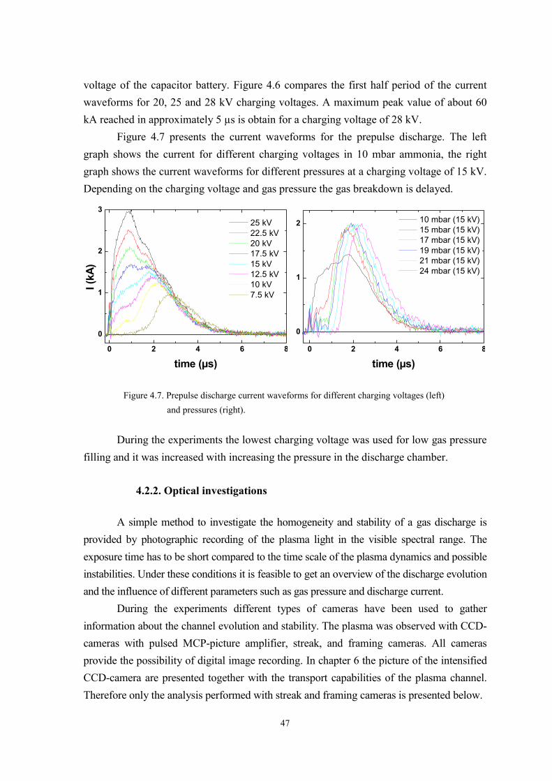
47

voltage of the capacitor battery. Figure 4.6 compares the first half period of the current waveforms for 20, 25 and 28 kV charging voltages. A maximum peak value of about 60 kA reached in approximately 5 µs is obtain for a charging voltage of 28 kV.

Figure 4.7 presents the current waveforms for the prepulse discharge. The left graph shows the current for different charging voltages in 10 mbar ammonia, the right graph shows the current waveforms for different pressures at a charging voltage of 15 kV. Depending on the charging voltage and gas pressure the gas breakdown is delayed.

0 2 4 6 8

0

1

2

3

I (kA

)

time (µs)

25 kV 22.5 kV 20 kV 17.5 kV 15 kV 12.5 kV 10 kV 7.5 kV

0 2 4 6 8

0

1

2

time (µs)

10 mbar (15 kV) 15 mbar (15 kV) 17 mbar (15 kV) 19 mbar (15 kV) 21 mbar (15 kV) 24 mbar (15 kV)

Figure 4.7. Prepulse discharge current waveforms for different charging voltages (left)

and pressures (right).

During the experiments the lowest charging voltage was used for low gas pressure filling and it was increased with increasing the pressure in the discharge chamber.

4.2.2. Optical investigations

A simple method to investigate the homogeneity and stability of a gas discharge is provided by photographic recording of the plasma light in the visible spectral range. The exposure time has to be short compared to the time scale of the plasma dynamics and possible instabilities. Under these conditions it is feasible to get an overview of the discharge evolution and the influence of different parameters such as gas pressure and discharge current.

During the experiments different types of cameras have been used to gather information about the channel evolution and stability. The plasma was observed with CCD-cameras with pulsed MCP-picture amplifier, streak, and framing cameras. All cameras provide the possibility of digital image recording. In chapter 6 the picture of the intensified CCD-camera are presented together with the transport capabilities of the plasma channel. Therefore only the analysis performed with streak and framing cameras is presented below.

48

Streak camera analysis of the plasma channel

Pictures of the discharge have been recorded with a Hamamatsu streak camera model C2830. A streak camera consists of three main units: imaging optics with an entrance slit, the streak tube, and imaging optics that transfers the picture from the phosphor screen of the streak tube to a readout system. The incident light is collected on the entrance slit and transferred to the photocathode of the streak tube using a relay lens. This slit image is converted to an electron image at the photocathode, is accelerated through the tube and passes a lateral deflection field, created by deflection plates. A sweeping voltage is applied to the plates when the electron image is passing through the field and causes a shift of the electron image from top to bottom. Next the electron image is intensified with a channel plate, and impinges upon a phosphor screen, where the electron image is reconverted into light. The resulting image is then generated on a CCD-chip by an output relay lens. As a result the image information on the streak slit is swept from top to bottom, which represents the time flow.

The streak images in figure 4.8 show straight, stable and symmetrically expanding channels. The temporal window of the streak camera is 14 µs. The slit of the streak camera is perpendicular to the discharge axis. The evolution of the channel radius is recorded in horizontal direction while the vertical direction represents the time flow.

-20 -10 0 10 2014

12

10

8

6

4

2

0

time

(µs)

radius (mm)

-20 -10 0 10 2014

12

10

8

6

4

2

0

time

(µs)

radius (mm)

Figure 4.8. Streak images of the discharge plasma in 21 mbar ammonia without (left) and with prepulse (right).

The horizontal profiles of the emitted light have been fitted with a Gaussian profile. The temporal evolution of the discharge radius measured as the half-width-at-half-maximum (FWHM/2) of the Gaussian profiles is presented in figure 4.9. The left graph

49

shows the radius evolution of discharges without prepulse and the right graph shows the radius evolution of discharges with prepulse.

0 1 2 3 40

2

4

6

8

10

without prepulse

radi

us (m

m)

time (µs)

2 mbar 7 mbar 12 mbar 14 mbar 17 mbar 21 mbar

0 1 2 3 4

with prepulse

time (µs)

2 mbar 7 mbar 12 mbar 14 mbar 17 mbar 21 mbar

Figure 4.9. Radius of the channel measured as the FWHM/2 of the light profile.

When the prepulse discharge is not used the channel radius decreases with

increasing pressure in the discharge chamber. When the prepulse is switched on almost no dependence of the evolutions on the pressures can be observed.

Streak images of the prepulse discharge for different pressures and charging voltages have revealed reproducible, stable and cylindrical symmetric plasma columns. Figure 4.10 shows typical streak images of the prepulse discharge for two different laser energy depositions in the background gas. The pressure in the chamber was 11 mbar and the capacitor was charged to 15 kV. In the left picture the laser has deposited about 1 J/cm2 and in the right picture about 1.4 J/cm2.

-10 0 1014

12

10

8

6

4

2

0

radius (mm)

time

(µs)

-10 0 1014

12

10

8

6

4

2

0

radius (mm)

time

(µs)

Figure 4.10. Streak pictures of a prepulse discharge in 11 mbar ammonia and 15 kV charging voltage

for 1 J/cm2 (left) and 1.4 J/cm2 (right) laser energy deposition.

50

Starting with 15 kV, for lower laser energy deposition, it looks that insulator breakdown occurs simultaneously and the current in the discharge is not increasing with voltage. This can happened if the laser beam creates on the axis almost the same conditions, as those needed for heaving breakdown towards the chamber walls. Therefore the light intensity is dimmer in the left picture of figure 4.10. The ammonia pressure was 11 mbar and laser has deposited about 1.4 J/cm2.

Figure 4.11. Evolution of the prepulse channel for a delay of 15 µs and 10 kV charging voltage (left) and a delay of 20 µs and 15 kV charging voltage (right).

A critical parameter in creating reproducible prepulse channels is the delay

between the laser beam pulse and the triggering of the discharge. For 10 µs delay the discharge has a very good reproducibility but when decreasing or increasing this delay, even with few microseconds, the discharge starts to behave as depicted in figure 4.11.

Framing camera analysis of the plasma channel

In the following section the channel evolution was investigated by means of a framing camera. A framing camera is able to acquire several frames with a short inter-frame delay. With such a camera studies of reproducibility or instabilities can be easily performed.

The optical appearance of the channel was studied in the pressure range from 10 to 21 mbar, without prepulse discharge. All six capacitors in the bank were charged at 20 kV for all pressures, leading to about 40 kA peak current in about 4.5 µs. The evolution of the plasma channel is presented in figure 4.12 for three representative pressures. The pictures show a section of about 3 cm from the whole channel, corresponding to the middle region. The first set of images is recorded at 14 mbar, the second at 18 mbar and the last at 21 mbar gas pressure. The two dotted lines, whereby the distance between two consecutive dots is 3 mm, give the scale of the pictures.

51

0.7 µs 1.7 µs 2.7 µs 3.7 µs 4.7 µs 5.7 µs

Figure 4.12. Framing camera images of the discharge at 14 mbar (top row), 18 mbar (middle row) and 21 mbar (bottom row) ammonia.

In the pressure range 10 to 17 mbar the channel presents no visible instabilities for

times longer than the time required for reaching the current maximum, i.e. 4.5 µs. For higher pressures the channel becomes unstable before the current maximum. Increasing the pressure reduces the time up to the onset of these instabilities significantly, from about 3.5 µs at 18 mbar to 2 µs at 21 mbar.

Since the channels have no defined edges the temporal evolution of the radial plasma channel motion was analyzed by fitting the vertical light intensity distribution with a Gaussian function. The width of the profile multiplied by a factor of 1.177 gives the full-width-at-half-maximum (FWHM) of the profile. In a first approximation this value was assumed as channel diameter and used to calculate the cross section through which the current flows homogeneously.

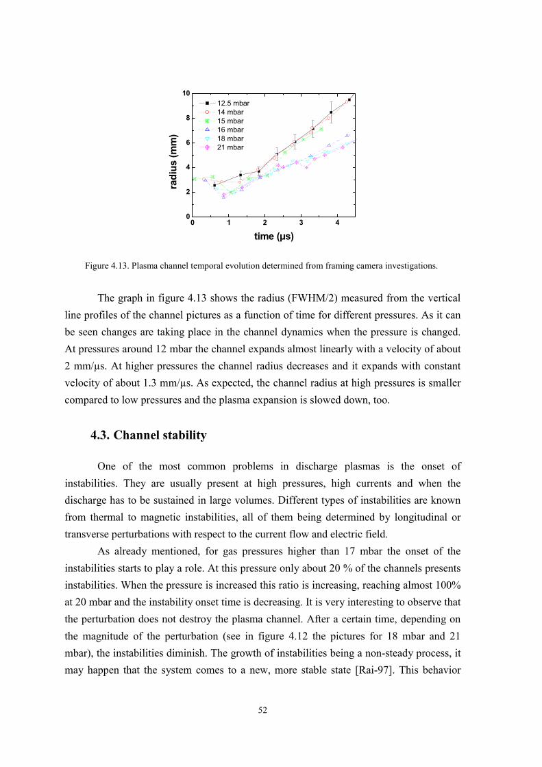
52

0 1 2 3 40

2

4

6

8

10

radi

us (m

m)

time (µs)

12.5 mbar 14 mbar 15 mbar 16 mbar 18 mbar 21 mbar

Figure 4.13. Plasma channel temporal evolution determined from framing camera investigations.

The graph in figure 4.13 shows the radius (FWHM/2) measured from the vertical

line profiles of the channel pictures as a function of time for different pressures. As it can be seen changes are taking place in the channel dynamics when the pressure is changed. At pressures around 12 mbar the channel expands almost linearly with a velocity of about 2 mm/µs. At higher pressures the channel radius decreases and it expands with constant velocity of about 1.3 mm/µs. As expected, the channel radius at high pressures is smaller compared to low pressures and the plasma expansion is slowed down, too.

4.3. Channel stability

One of the most common problems in discharge plasmas is the onset of instabilities. They are usually present at high pressures, high currents and when the discharge has to be sustained in large volumes. Different types of instabilities are known from thermal to magnetic instabilities, all of them being determined by longitudinal or transverse perturbations with respect to the current flow and electric field.

As already mentioned, for gas pressures higher than 17 mbar the onset of the instabilities starts to play a role. At this pressure only about 20 % of the channels presents instabilities. When the pressure is increased this ratio is increasing, reaching almost 100% at 20 mbar and the instability onset time is decreasing. It is very interesting to observe that the perturbation does not destroy the plasma channel. After a certain time, depending on the magnitude of the perturbation (see in figure 4.12 the pictures for 18 mbar and 21 mbar), the instabilities diminish. The growth of instabilities being a non-steady process, it may happen that the system comes to a new, more stable state [Rai-97]. This behavior

53

was also observed during the ion beam transport experiments. Even when the optical appearance of the discharge was not uniform, the images on the scintillator were indicating a linear field distribution inside the plasma column. A prepulse discharge had a beneficial effect on the channel stability at high pressures. First a capacitor of 40 nF showed an improvement. The instabilities appear much earlier now but the amplitude of the perturbation is lower. Next the capacity was increased to 200 nF. This improved the discharge behavior tremendously, allowing the increase of the current to peak values up to 60 kA for discharges in 20 mbar of ammonia. The discharge channels thus obtained show no instabilities, even at times of about 10 µs from the current start, i.e. the first zero of the current. An explanation could be the enhancement of the mass density of the gas wall enclosing the discharge channel by a radial shock wave launched when the prepulse discharge is ignited [Pon-01].

For the rarefaction channel created by laser heating the gas wall density ρg, is about 2.5 to 4 times higher then the channel gas density ρch [Nie-02b]. A shock wave generated by the prepulse discharge ignition leads to further rarefaction of the gas on the axis down to about 10% from the initial gas fill pressure. A decrease by almost one order of magnitude is expected in the growth rate of the m=1 type instability [Man-73]. The photographs of the channel nicely illustrate this effect. Figure 4.15 shows two pictures of a 40 kA the discharge recorded at about the same time for a gas fill pressure of 20 mbar ammonia without and with prepulse.

Figure 4.15. Fast gated camera pictures of the discharge channel in 20 mbar ammonia and 20 kV charging voltage. Discharge without pepulse (left) and with 15 kV prepulse (right).

The main bank was charged at 20 kV and after the breakdown of the gas the current

increases to 40 kA in about 5 µs. The left picture presents the channel at 3.54 µs for a discharge without prepulse while the right picture presents the channel at 3.82 µs in a discharge with 15 kV (3 kA peak current) prepulse discharge. With prepulse the plasma column shows no instabilities for at least the first-half period of the discharge. When the charging voltage is increased to 28 kV (about 60 kA peak current) the same behavior is found.

Calculating the growth rate of the instabilities in vacuum [Man-84] it is found that the instabilities should grow faster at lower pressure. In our experiments was observed

54

exactly the opposite. This can be explained if it is considered the stabilizing effect of the background gas that surrounds the discharge channel. After the CO2 laser pulse heats the gas, the mass density of the gas in the vicinity of the rarefaction channel created due to the gas expansion, is increased. Since the laser is depositing the same amount of energy in the gas for all pressures, the mass density of the gas wall formed at high pressure is lower compared to low pressure. Therefore when is calculated again the instabilities growth rate using the equation 2.29, that takes into account the effect of the background gas , it is found that the instabilities are growing faster with increasing the pressure.

4.4. Magnetic probe measurements

The radial distribution of the magnetic field can be accurately described if the exact position of the coils relative to the discharge channel axis is known. Therefore a fast-gated camera was used to acquire pictures of the discharge channel together with the probe for different times. The glass jacket of the probe reflects the light coming from the discharge. In this way it is easy to measure the position of the coils, as it can be seen from the pictures in figure 4.16.

Figure 4.16. Typical pictures used to determine the position of the probe relative to the discharge channel axis at different times, 1.22, 3.14 and 7.3 µs after the current start.

To check the influence of the magnetic probe on the discharge, interferograms of

the channel have been taken with the probe head immersed into the discharge, as shown in figure 4.17.

Figure 4.17. Interferometric images of the discharge channel with magnetic probe at 2.4, 3.9 and 5.4 µs after the current start.

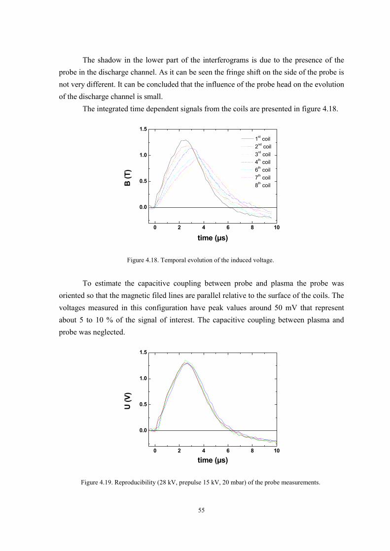
55

The shadow in the lower part of the interferograms is due to the presence of the probe in the discharge channel. As it can be seen the fringe shift on the side of the probe is not very different. It can be concluded that the influence of the probe head on the evolution of the discharge channel is small.

The integrated time dependent signals from the coils are presented in figure 4.18.

0 2 4 6 8 10

0.0

0.5

1.0

1.5

1st coil 2nd coil 3rd coil 4th coil 6th coil 7th coil 8th coil

B

(T)

time (µs)

Figure 4.18. Temporal evolution of the induced voltage.

To estimate the capacitive coupling between probe and plasma the probe was

oriented so that the magnetic filed lines are parallel relative to the surface of the coils. The voltages measured in this configuration have peak values around 50 mV that represent about 5 to 10 % of the signal of interest. The capacitive coupling between plasma and probe was neglected.

0 2 4 6 8 10

0.0

0.5

1.0

1.5

U (V

)

time (µs)

Figure 4.19. Reproducibility (28 kV, prepulse 15 kV, 20 mbar) of the probe measurements.

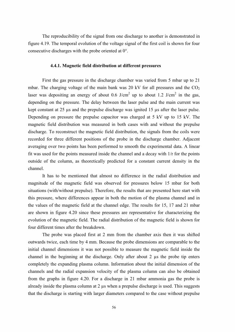
56

The reproducibility of the signal from one discharge to another is demonstrated in figure 4.19. The temporal evolution of the voltage signal of the first coil is shown for four consecutive discharges with the probe oriented at 0°.

4.4.1. Magnetic field distribution at different pressures

First the gas pressure in the discharge chamber was varied from 5 mbar up to 21

mbar. The charging voltage of the main bank was 20 kV for all pressures and the CO2 laser was depositing an energy of about 0.6 J/cm2 up to about 1.2 J/cm2 in the gas, depending on the pressure. The delay between the laser pulse and the main current was kept constant at 25 µs and the prepulse discharge was ignited 15 µs after the laser pulse. Depending on pressure the prepulse capacitor was charged at 5 kV up to 15 kV. The magnetic field distribution was measured in both cases with and without the prepulse discharge. To reconstruct the magnetic field distribution, the signals from the coils were recorded for three different positions of the probe in the discharge chamber. Adjacent averaging over two points has been performed to smooth the experimental data. A linear fit was used for the points measured inside the channel and a decay with 1/r for the points outside of the column, as theoretically predicted for a constant current density in the channel.

It has to be mentioned that almost no difference in the radial distribution and magnitude of the magnetic field was observed for pressures below 15 mbar for both situations (with/without prepulse). Therefore, the results that are presented here start with this pressure, where differences appear in both the motion of the plasma channel and in the values of the magnetic field at the channel edge. The results for 15, 17 and 21 mbar are shown in figure 4.20 since these pressures are representative for characterizing the evolution of the magnetic field. The radial distribution of the magnetic field is shown for four different times after the breakdown.

The probe was placed first at 2 mm from the chamber axis then it was shifted outwards twice, each time by 4 mm. Because the probe dimensions are comparable to the initial channel dimensions it was not possible to measure the magnetic field inside the channel in the beginning at the discharge. Only after about 2 µs the probe tip enters completely the expanding plasma column. Information about the initial dimension of the channels and the radial expansion velocity of the plasma column can also be obtained from the graphs in figure 4.20. For a discharge in 21 mbar ammonia gas the probe is already inside the plasma column at 2 µs when a prepulse discharge is used. This suggests that the discharge is starting with larger diameters compared to the case without prepulse

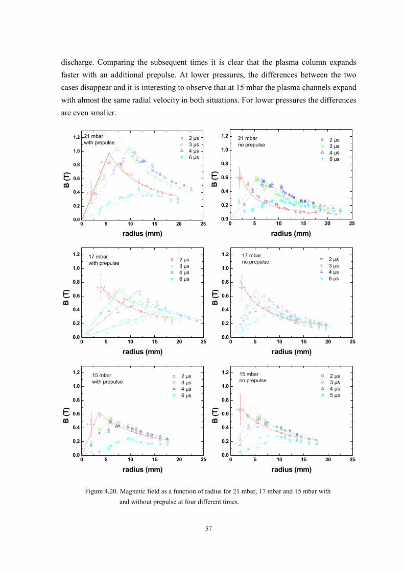
57

discharge. Comparing the subsequent times it is clear that the plasma column expands faster with an additional prepulse. At lower pressures, the differences between the two cases disappear and it is interesting to observe that at 15 mbar the plasma channels expand with almost the same radial velocity in both situations. For lower pressures the differences are even smaller.

0 5 10 15 20 250.0

0.2

0.4

0.6

0.8

1.0

1.2 21 mbarwith prepulse

B (T

)

radius (mm)

2 µs 3 µs 4 µs 6 µs

0 5 10 15 20 250.0

0.2

0.4

0.6

0.8

1.0

1.2 21 mbarno prepulse

B (T

)

radius (mm)


0 5 10 15 20 250.0

0.2

0.4

0.6

0.8

1.0


B (T

)

radius (mm)


0 5 10 15 20 250.0

0.2

0.4

0.6

0.8

1.0


B (T

)

radius (mm)


0 5 10 15 20 250.0

0.2

0.4

0.6

0.8

1.0


B (T

)

radius (mm)


0 5 10 15 20 250.0

0.2

0.4

0.6

0.8

1.0


B (T

)

radius (mm)


Figure 4.20. Magnetic field as a function of radius for 21 mbar, 17 mbar and 15 mbar with

and without prepulse at four different times.

58

Another important observation is the fact that the magnetic field strength increases with the pressure when a prepulse discharge is used, while it remains almost constant when the prepulse discharge is not present. But, the magnetic field gradient depends on both the field strength and the channels radius. Because of a larger channel radius, the magnetic field gradient generated when using a prepulse discharge does not reach a higher peak value than the magnetic field gradient created in discharges without prepulse, at the same gas pressure. This observation holds for high-pressure operation. The two major advantages when using a prepulse discharge are that the channel stability improves and that the channel expands faster and is therefore matching the ion beam diameter faster than without prepulse.

4.4.2. Magnetic field distribution at different charging voltages Keeping the pressure constant at 20 mbar the voltage was varied from 20 to 28 kV

in three steps. The current measured with the external shunt results in values of the current increasing from 45 to 60 kA. Figure 4.21 presents the radial distribution of the magnetic field for 28 and 25 kV charging voltage with prepulse for four different times after the ignition of the discharge. A linear fit was used for the points measured inside the channel and decay with 1/r for the points measured outside the column. As expected, the magnetic field is increasing with increasing voltage but simultaneously the radial expansion velocity of the plasma is also increasing. Therefore the magnetic field gradient inside the plasma channel does not reach higher values, but it remains constant when the discharge current is increased. This phenomenon was also observed during the transport experiments.

0 5 10 15 20 250.0

0.5

1.0

1.5

2.0

B (T

)

radius (mm)


0 5 10 15 20 250.0

0.5

1.0

1.5

2.0

B (T

)

radius (mm)


Figure 4.21. Radial distribution of the magnetic field for discharge channels created in 20 mbar

gas pressure for 28 and 25 kV charging voltage with prepulse.

59

Because of the spatial resolution of the magnetic probes which is limited to about 1 mm due to the coil diameter, the peak magnetic field values can be 25 % higher than shown in figure 4.21

The most important information that can be extracted from figure 4.21 is the linear increase of the magnetic field inside the plasma channel. Thus the current is uniformly distributed along the discharge channel radius.

4.4.3. Discussions

The current flowing in the discharge channel creates magnetic fields at the edge

that have values as high as 1.5 T. For the ion beam transport the gradient of the field inside the channel is important which is inversely proportional to the square of the channel radius. Small changes in the radius are leading to large variations of the magnetic field gradient. Therefore the most important parameter that has to be observed is the radius of the channel current distribution and its evolution in time. The temporal evolution of the channel radius for different pressures is shown in figure 4.22. The full symbols are representing discharges with prepulse and the hollow symbols represent discharges without prepulse. The same line type is used to represent the same pressure. The right side of the same figure shows the calculated magnetic field gradient assuming homogeneous current distribution.

0 1 2 3 4 5 60

5

10

15

20

radi

us (m

m)

time (µs)

15 mbar /prepulse 15 mbar 17 mbar /prepulse 17 mbar 21 mbar / prepulse 21 mbar

2 3 4 5 60

50

100

150

200

250

G (T

/m)

time (µs)

15 mbar /prepulse 15 mbar 17 mbar /prepulse 17 mbar 21 mbar /prepulse 21 mbar

Figure 4.22. Radius of the plasma channel (left) and magnetic field gradient (right) as determined

from magnetic field measurements for a discharge voltage of 20 kV.

An interesting feature in the left graph of figure 4.22 is the observation that,

independent of the pressure, the channel radius increases with the same velocity for

60

discharges without prepulse. When a prepulse discharge is used the channel expands approximately with the same rate but the radii are higher and they increase with pressure from 15 to 21 mbar. With increasing discharge current but a constant gas pressure of 21 mbar the channels expand faster but almost the same magnetic field gradient strengthens is achieved (figure 4.23).

0 1 2 3 4 5 6

5

10

15

20

radi

us (m

m)

time (µs)

20 kV 25 kV 28 kV

0 1 2 3 4 5 60

50

100

150

200

250

G (T

/m)

time (µs)

20 kV 25 kV 28 kV

Figure 4.23. Radius of the plasma channel (left) and magnetic field gradient (right) for 20, 25 and 28 kV

charging voltages of the main bank for 20 mbar ammonia with prepulse. Although a quantitative analysis of the magnetic field gradient cannot be

performed it has to be observed that the maximum value is reached earlier than 2 µs after ignition. This is important for the transport experiments where the radius of the channel has to match the ion beam dimensions while a sufficiently strong field gradient is generated.

A mean current density is calculated applying equation 2.47 and the results are given in figure 4.24. The top row of this figure shows the radial distribution of the current for a 40 kA discharge in 17 mbar for different times with (a) and without prepulse (b). The prepulse current was about 2 kA. The lower row of the same figure presents the radial distribution of the current density at constant gas pressure for different discharge currents, i.e. 60 kA (c) and 50 kA (d). A discharge current of 60 kA corresponds to 28 kV charging voltage, while 50 kA corresponds to 25 kV.

The values of the current density range from about 5107 A/m2 to about 3108 A/m2

but are rather scattered. The current density can reach peak values as high as 3108 A/m2 at the current maximum, i.e. about 4 µs from the current start. The errors related to the method used for this estimation are large. Under these conditions, a uniform current density distribution could be assumed. For 17 mbar without prepulse a different, non-uniform distribution seems to be more appropriate.

61

0 5 10 150

10

20

30

40

50

j * 1

07 (A/m

2 )

radius (mm)

3 µs 4 µs 6 µs

0 5 10 15

0

10

20

30

40

50

j *10

7 (A/m

2 )

radius (mm)

3 µs 4 µs 6 µs

(a) (b)

0 5 10 15 20

10

20

30

40

50

j * 1

07 (A/m

2 )

radius (mm)

3 µs 4 µs 6 µs

0 5 10 15 20

10

20

30

40

50

j * 1

07 (A/m

2)

radius (mm)

3 µs 4 µs 5 µs

(c) (d)

Figure 4.24. Current density for a discharge in 17 mbar ammonia with (a) and without (b) prepulse. Current densities for 28 and 25 kV charging voltage (c) and (d), respectively.

The current values determined from the magnetic field decay outside the plasma

channel are in good agreement with the current values measured with the external shunt. This shows that almost all the current flows inside the channel boundaries.

An example is given in figure 4.25 for a pressure of 17 mbar and a current peak value of about 40 kA. This figure presents current waveforms for discharges with (left) and without prepulse (right). It can be seen that the magnetic probe measurements of the current are in good agreement with the values measured with the current shunt.

62

0 2 4 6 8-60

-40

-20

0

I (

A)

time (µs)

shunt magnetic probe

0 2 4 6 8-60

-40

-20

0

I (A)

time (mm)

shunt magnetic probe

Figure 4.25. Current waveforms measured with shunt (black full symbols) and magnetic probe

(red hollow symbols) for 17 mbar ammonia without (left) and with (right) prepulse.

It is not clear why all values are either smaller or higher for discharges with or

without prepulse. A reason may be a different shape of the current density distribution in these two situations or a slightly different interaction between the probe-and the plasma channel, but more investigations are required to find a precise explanation.

heavy ion beam transport in laser initiated high … ion beam transport in laser initiated high...

Documents