heat conduction simulation of 2d moving heat source...

Research ArticleHeat Conduction Simulation of 2D Moving Heat Source ProblemsUsing a Moving Mesh Method

Zhicheng Hu and Zhihui Liu

Department of Mathematics, College of Science, Nanjing University of Aeronautics and Astronautics, Nanjing 210016, China

Correspondence should be addressed to Zhicheng Hu; [email protected]

Received 4 January 2020; Accepted 27 January 2020; Published 11 February 2020

Academic Editor: Soheil Salahshour

Copyright © 2020 Zhicheng Hu and Zhihui Liu. This is an open access article distributed under the Creative Commons AttributionLicense, which permits unrestricted use, distribution, and reproduction in any medium, provided the original work isproperly cited.

This paper focuses on efficiently numerical investigation of two-dimensional heat conduction problems of material subjected tomultiple moving Gaussian point heat sources. All heat sources are imposed on the inside of material and assumed to movealong some specified straight lines or curves with time-dependent velocities. A simple but efficient moving mesh method, whichcontinuously adjusts the two-dimensional mesh dimension by dimension upon the one-dimensional moving mesh partialdifferential equation with an appropriate monitor function of the temperature field, has been developed. The physical modelproblem is then solved on this adaptive moving mesh. Numerical experiments are presented to exhibit the capability of theproposed moving mesh algorithm to efficiently and accurately simulate the moving heat source problems. The transient heatconduction phenomena due to various parameters of the moving heat sources, including the number of heat sources and thetypes of motion, are well simulated and investigated.

1. Introduction

Heat conduction phenomena of material involving movingheat sources, which have attracted increasing attention byscientists and engineers in the past few decades, have beenstudied in a wide range of fields, such as welding, cutting,drilling, laser hardening/forming, plasma spraying, heattreating of metals, manufacturing of electronic components,and even firing a gun barrel, solid propellant burning, anddental treatment, see e.g., [1–5] and references therein.The most important physical quantity of interest for suchpractical applications is the temperature field of themedium, which is usually modeled by the heat conductionequation with time-dependent localized source terms formoving heat sources. Once the temperature field isobtained, many other thermophysical properties of mate-rial, including metallurgical microstructures, thermal stress,residual stress, and part distortion, could be subsequentlydetermined [6–10]. It is therefore particularly importantto precisely and efficiently predict the dynamic variationof the temperature field around the moving heat sourcesduring these engineering processes.

In order to investigate the temperature field and therelated thermal properties of the problem with moving heatsources, numerous methods, in either analytical or numericalapproach, have been developed, since the 1930s, when thepioneering work of Rosenthal was proposed for the analyticalsolution of a simplified moving heat source problem [11].Although analytical methods are still popular nowadays[12], they are usually only available for simple situations suchas the quasistationary problem of a single heat source movingalong a straight line with a constant speed. In comparison toanalytical methods, numerical methods could only provideresults approximately within an acceptable error tolerance,but they are more flexible to deal with the complicated yetpractical situations such as the transient problem of multipleheat sources moving in a complex geometry of the materialwith time-dependent speeds [3]. However, most of numericalstudies, regardless using meshless methods [13, 14] or mesh-based methods such as the finite element method [6, 10],were concerned about problems involving only a heat sourcemoving along a straight line with a constant speed, or multi-ple heat sources moving along parallel straight lines with thesame constant speed. Apart from these, the technique of

HindawiAdvances in Mathematical PhysicsVolume 2020, Article ID 6067854, 16 pageshttps://doi.org/10.1155/2020/6067854

https://orcid.org/0000-0002-5523-5152

https://creativecommons.org/licenses/by/4.0/






https://doi.org/10.1155/2020/6067854

moving coordinate system, such that the heat source is sta-tionary in the new coordinate system, is often introduced inboth analytical and numerical analyses of the quasistationaryproblem [1, 13]. Nevertheless, it is obvious that this tech-nique is limited and not applicable for problems subjectedto multiple moving heat sources with different velocitiesand trajectories.

It is well known that the moving heat source might beimposed on the surface or inside of material [2], which fol-lows that the resulting mathematical model would contain asource term in the boundary condition or the governing heatconduction equation, respectively. Depending on the practi-cal applications, the moving heat source can be modeled asa point, line, or plane source with various geometries, suchas square, circle, semiellipsoidal and double ellipsoidal [1,15, 16]. No matter what kind of the moving heat source, itsenergy is always highly concentrated in a time-dependentlocalized domain. It turns out that the resulting temperatureof material would change drastically in the localized regionaround the moving heat source. Consequently, it is obviousthat a significant improvement in efficiency could beachieved, if an adaptive mesh method, which concentrates anumber of mesh points dynamically in the local regions ofrapid variation of the temperature, is employed to solve theproblem with the same accuracy as the fixed mesh method.

The moving mesh method [17, 18] is one of the popularadaptive methods and has been successfully applied to vari-ous problems that contain time-dependent localized singu-larities [19–21]. It usually tries to find a time-dependentone-to-one coordinate transformation between the physicaldomain and the computational domain, by solving an addi-tional system of moving mesh partial differential equation(MMPDE), which equidistributes a certain monitor func-tion of the physical solution [22, 23]. The original physicalequation would be subsequently transformed into the com-putational domain and then be solved by the standard uni-form mesh method. For more details of the moving meshmethod, one is referred to [17, 23, 24]. Up to now, themoving mesh method has been exhibited to work well forproblems with moving heat source in a one-dimensional(1D) case [25, 26]. Yet the application of the moving meshmethod to the problem of moving heat source in multidi-mensional case is still immature.

Based on the above observations, this paper is concernedabout the efficiently numerical study of two-dimensional(2D) heat conduction problems involving multiple movingheat sources by the moving mesh method. The Gaussianpoint heat source, that is imposed on the inside of materialand allowed to move along any specified curve with a time-dependent velocity, is taken for all heat sources as an exampleof the model problem. A simple moving mesh method, whichgenerates the 2D moving mesh dimension by dimensionfrom 1D MMPDE with an appropriately defined monitorfunction, is developed. The transient heat conduction phe-nomena due to various parameters of the moving heatsources, such as the number of heat sources and the typesof motion, are then investigated with the proposed movingmesh method. Since only two additional 1D systems arerequired to be solved, the resulting moving mesh method is

easy to be implemented and turns out to be very efficient togive satisfactory results.

The rest of the paper is outlined as follows. In Section 2,the mathematical model of the 2D heat conduction problemwith multiple moving heat sources is briefly introduced. Thedetailed formulation of the moving mesh method for themodel problem is described in Section 3. Numerical experi-ments are presented to show the efficiency of the proposedmoving mesh method in Section 4, where heat conductionphenomena are also investigated in detail. Finally, some con-clusions are given in the last section.

2. Mathematical Model

In a thin rectangular plate made of homogeneous material,heat flow can be simplified to be viewed as a two-dimensional flow. Let the plate occupy domain Ω = fðx, yÞ:− Lx/2 ≤ x ≤ Lx/2,−Ly/2 ≤ y ≤ Ly/2g, where Lx and Ly are thelength and width of the plate, respectively. Suppose the plateis initially at room temperature denoted by T0 and is heatedby several moving heat sources at time t > 0, as shown inFigure 1. Then using Tðx, y, tÞ to represent the temperatureat position ðx, yÞ and time t, the evolution of the temperaturein the plate can be described by the following two-dimensional heat conduction equation:

ρc∂T∂t

− k∂2T∂x2

+ ∂2T∂y2

!= 〠

q

l=1gl x, y, tð Þ, x, yð Þ ∈Ω, t > 0,

ð1Þ

where ρ, c, and k are the material density, the heat capacity,and the thermal conductivity, respectively. In the currentinvestigation, these quantities are assumed to be constantindependent of the position and temperature. The right-hand side of (1) represents the heat source term, where q isthe number of heat sources and glðx, y, tÞ is the volumetricheat generation rate of the lth heat source.

Depending on the physical nature of the problem, amoving heat source can be roughly classified into threetypes, namely, the point, line, and plane heat source. Allof them concentrate high power in a time-dependentlocalized region and can be well modeled by a Dirac delta

Moving path

Heat source

Lx

Ly

Figure 1: Sketch of the rectangular plate with a moving pointheat source.

2 Advances in Mathematical Physics

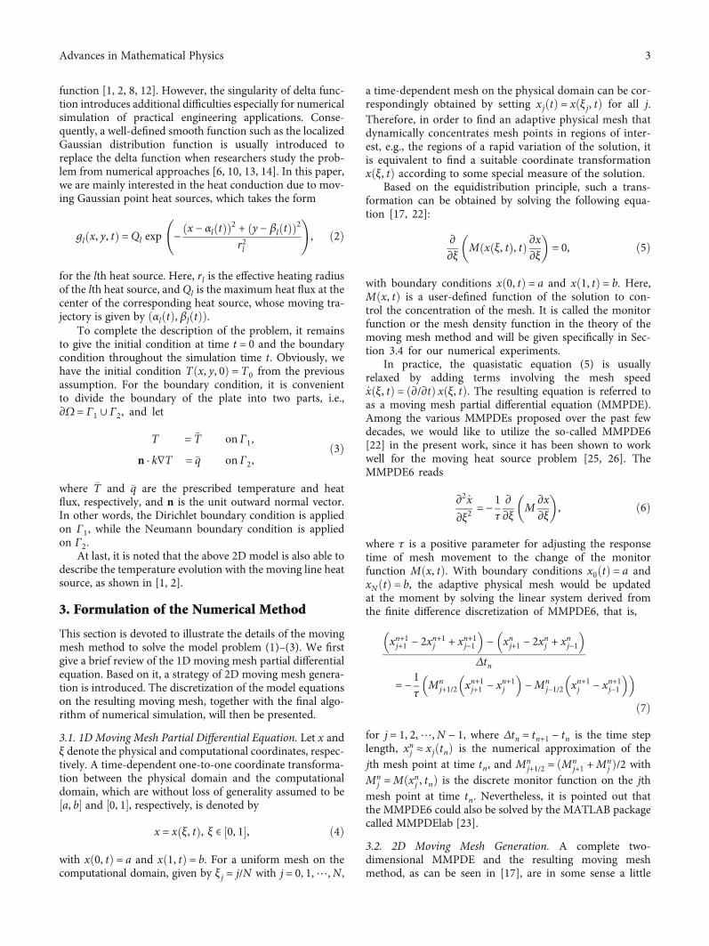
function [1, 2, 8, 12]. However, the singularity of delta func-tion introduces additional difficulties especially for numericalsimulation of practical engineering applications. Conse-quently, a well-defined smooth function such as the localizedGaussian distribution function is usually introduced toreplace the delta function when researchers study the prob-lem from numerical approaches [6, 10, 13, 14]. In this paper,we are mainly interested in the heat conduction due to mov-ing Gaussian point heat sources, which takes the form

gl x, y, tð Þ =Ql exp −x − αl tð Þð Þ2 + y − βl tð Þð Þ2

r2l

!, ð2Þ

for the lth heat source. Here, rl is the effective heating radiusof the lth heat source, and Ql is the maximum heat flux at thecenter of the corresponding heat source, whose moving tra-jectory is given by ðαlðtÞ, βlðtÞÞ.

To complete the description of the problem, it remainsto give the initial condition at time t = 0 and the boundarycondition throughout the simulation time t. Obviously, wehave the initial condition Tðx, y, 0Þ = T0 from the previousassumption. For the boundary condition, it is convenientto divide the boundary of the plate into two parts, i.e.,∂Ω = Γ1 ∪ Γ2, and let

T = �T onΓ1,n · k∇T = �q onΓ2,

ð3Þ

where �T and �q are the prescribed temperature and heatflux, respectively, and n is the unit outward normal vector.In other words, the Dirichlet boundary condition is appliedon Γ1, while the Neumann boundary condition is appliedon Γ2.

At last, it is noted that the above 2D model is also able todescribe the temperature evolution with the moving line heatsource, as shown in [1, 2].

3. Formulation of the Numerical Method

This section is devoted to illustrate the details of the movingmesh method to solve the model problem (1)–(3). We firstgive a brief review of the 1D moving mesh partial differentialequation. Based on it, a strategy of 2D moving mesh genera-tion is introduced. The discretization of the model equationson the resulting moving mesh, together with the final algo-rithm of numerical simulation, will then be presented.

3.1. 1D Moving Mesh Partial Differential Equation. Let x andξ denote the physical and computational coordinates, respec-tively. A time-dependent one-to-one coordinate transforma-tion between the physical domain and the computationaldomain, which are without loss of generality assumed to be½a, b� and ½0, 1�, respectively, is denoted by

x = x ξ, tð Þ, ξ ∈ 0, 1½ �, ð4Þ

with xð0, tÞ = a and xð1, tÞ = b. For a uniform mesh on thecomputational domain, given by ξj = j/N with j = 0, 1,⋯,N,

a time-dependent mesh on the physical domain can be cor-respondingly obtained by setting xjðtÞ = xðξj, tÞ for all j.Therefore, in order to find an adaptive physical mesh thatdynamically concentrates mesh points in regions of inter-est, e.g., the regions of a rapid variation of the solution, itis equivalent to find a suitable coordinate transformationxðξ, tÞ according to some special measure of the solution.

Based on the equidistribution principle, such a trans-formation can be obtained by solving the following equa-tion [17, 22]:

∂∂ξ

M x ξ, tð Þ, tð Þ ∂x∂ξ� �

= 0, ð5Þ

with boundary conditions xð0, tÞ = a and xð1, tÞ = b. Here,Mðx, tÞ is a user-defined function of the solution to con-trol the concentration of the mesh. It is called the monitorfunction or the mesh density function in the theory of themoving mesh method and will be given specifically in Sec-tion 3.4 for our numerical experiments.

In practice, the quasistatic equation (5) is usuallyrelaxed by adding terms involving the mesh speed_xðξ, tÞ = ð∂/∂tÞ xðξ, tÞ. The resulting equation is referred toas a moving mesh partial differential equation (MMPDE).Among the various MMPDEs proposed over the past fewdecades, we would like to utilize the so-called MMPDE6[22] in the present work, since it has been shown to workwell for the moving heat source problem [25, 26]. TheMMPDE6 reads

∂2 _x∂ξ2

= −1τ

∂∂ξ

M∂x∂ξ

� �, ð6Þ

where τ is a positive parameter for adjusting the responsetime of mesh movement to the change of the monitorfunction Mðx, tÞ. With boundary conditions x0ðtÞ = a andxNðtÞ = b, the adaptive physical mesh would be updatedat the moment by solving the linear system derived fromthe finite difference discretization of MMPDE6, that is,

xn+1j+1 − 2xn+1j + xn+1j−1

� �− xnj+1 − 2xnj + xnj−1� �

Δtn

= −1τ

Mnj+1/2 xn+1j+1 − xn+1j

� �−Mn

j−1/2 xn+1j − xn+1j−1

� �� ð7Þ

for j = 1, 2,⋯,N − 1, where Δtn = tn+1 − tn is the time steplength, xnj ≈ xjðtnÞ is the numerical approximation of thejth mesh point at time tn, and Mn

j+1/2 = ðMnj+1 +Mn

j Þ/2 withMn

j =Mðxnj , tnÞ is the discrete monitor function on the jthmesh point at time tn. Nevertheless, it is pointed out thatthe MMPDE6 could also be solved by the MATLAB packagecalled MMPDElab [23].

3.2. 2D Moving Mesh Generation. A complete two-dimensional MMPDE and the resulting moving meshmethod, as can be seen in [17], are in some sense a little

3Advances in Mathematical Physics

complicated and not easy to use. On the other hand, an adap-tive rectangular mesh on the physical domain generated by1D mesh strategy is obviously much simpler and has alsobeen successfully applied to reaction-diffusion equations ofquenching type, see e.g. [19, 27]. Accordingly, we shall followthe later approach to generate the adaptive rectangular meshon the physical domain via 1D MMPDE dimension bydimension in this paper.

To be specific, let the time-dependent one-to-one coor-dinate transformation between 1D domains ½−Lx/2, Lx/2�and ½0, 1� be still denoted by x = xðξ, tÞ with xð0, tÞ = −Lx/2and xð1, tÞ = Lx/2. Given a uniform mesh on thedomain ½0, 1� with ξi = i/Nx for i = 0, 1,⋯,Nx , a time-dependent mesh on the domain ½−Lx/2, Lx/2� could beobtained by setting xiðtÞ = xðξi, tÞ for all i. Similarly, byintroducing a time-dependent one-to-one coordinate trans-formation y = yðη, tÞ with yð0, tÞ = −Ly/2 and yð1, tÞ = Ly/2between 1D domains ½−Ly/2, Ly/2� and ½0, 1�, a time-dependent mesh on the domain ½−Ly/2, Ly/2� could beobtained by yjðtÞ = yðηj, tÞ, where η j = j/Ny with j = 0, 1,⋯,Ny is the uniform mesh on the domain ½0, 1�. Then a time-dependent rectangular mesh on the physical domain Ωwould be generated by setting the mesh point to be ðxiðtÞ,yjðtÞÞ for all i and j.

As stated in the previous subsection, both xiðtÞ and yjðtÞcan be determined from 1D MMPDE6 by utilizing appropri-ate monitor functions Mðx, tÞ and Gðy, tÞ, respectively,where Mðx, tÞ and Gðy, tÞ are functions of the 2D solutionTðx, y, tÞ, and will be specified in Section 3.4.

Obviously, the above strategy of 2D moving meshgeneration is very efficient and easy to be implemented,since only two one-dimensional linear systems are needto be solved.

3.3. Discretization on the Moving Mesh. It is now ready tointroduce the discretization of the model equations (1)–(3)on the 2D rectangular moving mesh using the central finitedifference method.

Using the time-dependent coordinate transformationsx = xðξ, tÞ and y = yðη, tÞ between the physical coordinatesx, y and the computational coordinates ξ, η, any functionof x, y, and t can be expressed as a function in terms of ξ,η, and t, that is, f ðx, y, tÞ = f ðxðξ, tÞ, yðη, tÞ, tÞ. By thechain rule, it follows that

∂f∂ξ

= ∂f∂x

∂x∂ξ

, ∂f∂η

= ∂f∂y

∂y∂η

, ∂f∂t ξ,ηfixed =

∂f∂t

��x,yfixed

+ ∂f∂x

_x ξ, tð Þ + ∂f∂y

_y η, tð Þ:

ð8Þ

In order to distinguish the two partial derivatives withrespect to t in the above expression, the notation _f , similarto the notation of mesh speed _x, is introduced for the firstone, i.e., _f = ∂f /∂tjξ,ηfixed, and the other one is simplified tothe original notation ∂f /∂t without causing confusion.Then, in the computational coordinates ξ, η ∈ ½0, 1� andt > 0, the original physical equation (1) becomes

_T −∂T∂ξ

/ ∂x∂ξ

� �_x −

∂T∂η

/ ∂y∂η

� �_y

− μ∂∂ξ

∂T∂ξ

/ ∂x∂ξ

� �/ ∂x∂ξ

+ ∂∂η

∂T∂η

/ ∂y∂η

� �/ ∂y∂η

� �= ~g ξ, η, tð Þ,

ð9Þ

where μ = k/ðρcÞ is the thermal diffusivity and ~gðξ, η, tÞ =1/ðρcÞ∑q

l=1 glðxðξ, tÞ, yðη, tÞ, tÞ.The above equation can be discretized using the second-

order central finite difference method on the uniform com-putational mesh ðξi, ηjÞ with i = 0, 1,⋯,Nx and j = 0, 1,⋯,Ny . This subsequently yields a system of ordinary differentialequations of the form

_Ti,j −A i,j tð Þ _xi −Bi,j tð Þ _yj −L i,j tð Þ = 0,i = 1, 2,⋯,Nx − 1, j = 1, 2,⋯,Ny − 1,

ð10Þ

where Ti,j = Ti,jðtÞ = Tðξi, ηj, tÞ, xi = xiðtÞ, yj = yjðtÞ, and

A i,j tð Þ=Ti+1,j tð Þ − Ti−1,j tð Þxi+1 tð Þ − xi−1 tð Þ , Bi, j tð Þ =

Ti,j+1 tð Þ − Ti,j−1 tð Þyj+1 tð Þ − yj−1 tð Þ ,

L i,j tð Þ= μ2

xi+1 tð Þ − xi−1 tð ÞTi+1,j tð Þ − Ti, j tð Þxi+1 tð Þ − xi tð Þ

−Ti,j tð Þ − Ti−1,j tð Þxi tð Þ − xi−1 tð Þ

� ��

+ 2yj+1 tð Þ − yj−1 tð Þ

Ti,j+1 tð Þ − Ti,j tð Þyj+1 tð Þ − yj tð Þ

−Ti,j tð Þ − Ti,j−1 tð Þyj tð Þ − yj−1 tð Þ

!#

+ ~g ξi, ηj, t� �

:

ð11Þ

Using the Crank-Nicolson method for temporal discreti-zation, a full discretization, which has second-order timeaccuracy, can be obtained by

Tn+1i,j − Tn

i,jΔtn

−An

i,j +An+1i,j

2xn+1i − xni

Δtn

−Bn

i,j +Bn+1i,j

2yn+1j − ynj

Δtn−Ln

i,j +Ln+1i,j

2 = 0,ð12Þ

for i = 1, 2,⋯,Nx − 1 and j = 1, 2,⋯,Ny − 1. In the aboveequation, Tn

i,j ≈ Ti,jðtnÞ is the numerical approximation ofthe temperature at ðξi, η jÞ at time tn, equivalently at ðxni , ynj Þof the physical domain at time tn. As for A

ni,j, B

ni,j, and Ln

i,j,they are numerical approximations of A i,jðtnÞ, Bi,jðtnÞ,and L i,jðtnÞ, respectively, and computed by substitutingall time-dependent quantities with the correspondingnumerical approximations in (11). Similarly, Tn+1

i,j , An+1i,j ,

Bn+1i,j , and Ln+1

i,j are corresponding numerical approxima-tions at time tn+1.

Supplemented with appropriate discretization ofboundary condition (3), the linear system (12) can thenbe solved for all Tn+1

i,j . Let us take the left boundary wherex = −Lx/2 or equivalently ξ = 0 as an example. If on the left


boundary it is subjected to the Dirichlet boundary condi-tion, we shall directly set

Tn+10,j = �T , ð13Þ

for all j. Alternatively, if on the left boundary it is sub-jected to the Neumann boundary condition, whichreduces to

−k∂T∂x

= �q, ð14Þ

we shall take the following discretization:

Tn+11,j − Tn+1

0,jxn+11 − xn+10

+Tn+12,j − Tn+1

0,jxn+12 − xn+10

−Tn+12,j − Tn+1

1,jxn+12 − xn+11

= −�qk

ð15Þ

for all j, to make sure the discretization of the boundarycondition is also second-order accuracy.

3.4. Final Algorithm and the Monitor Function. Now, we arein a position to describe the whole numerical algorithm thatsimulates the moving heat source problem with the movingmesh method. It is evident that the full discretization, includ-ing the system of the discretization (12) and the discretiza-tion of two 1D MMPDE6 for xn+1i and yn+1j , respectively, iscoupled together via the monitor functions and the physicalmesh. A simple decouple strategy is adopted in the presentalgorithm, that is, the mesh equation and the physical equa-tion are solved alternately one by one. A flowchart of the finalmoving mesh algorithm is then presented in Algorithm 1.However, to close this section, it remains to give the detailsof the monitor functions Mn

i and Gnj .

It is well known that the monitor function plays animportant role to the success of the moving mesh method[17]. One of the popular choices is the arc-length monitorfunction, which is aimed at equidistributing the arc-lengthof the solution curve between each two adjacent mesh points.As a result, it usually works well and is able to concentrate themesh points in the local regions of a large derivative of thesolution. Additionally, if there are local regions with large

curvature of the solution, then the curvature monitor func-tion might be a good candidate.

For the moving heat source problem, it is easy to showthat there are not only local regions with large derivativesof the solution but also local regions, e.g., the neighbor-hood of the point heat source, where the curvature ofthe solution is large and the derivative is close to 0. Inview of these, a linear combination of the arc-length mon-itor function and the curvature monitor function, whichreads

M x, tð Þ = θ

ffiffiffiffiffiffiffiffiffiffiffiffiffiffiffiffiffiffiffiffiffi1 + ∂u

∂x

� �2s

+ 1 − θð Þ

ffiffiffiffiffiffiffiffiffiffiffiffiffiffiffiffiffiffiffiffiffiffiffiffi1 + ∂2u

∂x2

!24

vuut , ð16Þ

is employed in our numerical experiments. Here, u = uðx, tÞis a 1D function defined later by a certain average of the2D temperature Tðx, y, tÞ with respect to y, and θ is theweight of the arc-length monitor function. Applying thecentral finite difference method to (16), one can obtainMn

i on xni by

Mni = θ

ffiffiffiffiffiffiffiffiffiffiffiffiffiffiffiffiffiffiffiffiffiffiffiffiffiffiffiffiffiffiffiffiffiffiffiffi1 + uni+1 − uni−1

xni+1 − xni−1

� �2s

+ 1 − θð Þffiffiffiffiffiffiffiffiffiffiffiffiffiffiffiffiffiffiffiffiffiffiffiffiffiffiffiffiffiffiffiffiffiffiffiffiffiffiffiffiffiffiffiffiffiffiffiffiffiffiffiffiffiffiffiffiffiffiffiffiffiffiffiffiffiffiffiffiffiffiffiffiffiffiffiffiffiffiffiffiffiffi1 + 2

xni+1 − xni−1

uni+1 − unixni+1 − xni

−uni − uni−1xni − xni−1

� �� 24

s,

ð17Þ

where uni = uðxni , tnÞ. Apparently, it is enough to give uniin the computation of Mn

i . Taking the whole 2D temper-ature field into consideration, the value of uni may bedefined by

uni =1

Ny + 1〠Ny

j=0Tni,j: ð18Þ

Furthermore, it is pointed out in [17] that the smoothnessof the monitor function may affect the stability and quality of

Input: The end time tend , initial physical mesh (x0i , y0j ) and initial temperature field T0

i, j.Output: The final physical mesh (xni , y

nj ) and the corresponding temperature field Tn

i,j.1 Let n = 0 and tn = 0;2 while tn < tend do3 Determine the time step Δtn;4 Compute the 1D monitor functionsMn

i on xni for all i, and Gnj on ynj for all j, based on the current physical mesh (xni , y

nj ) and the

corresponding temperature field Tni,j;

5 Solve two linear systems of discretization of 1D MMPDE6 withMni and G

nj , respectively, to get two new 1D mesh xn+1i and yn+1j ;

6 Construct the new physical mesh (xn+1i , yn+1j );

7 Solve the system of discretization (12) to get the new temperature field Tn+1i,j ;

8 Let tn+1 = tn + Δtn and n≔ n + 1;9 end

Algorithm 1. Flowchart of the moving mesh algorithm for moving heat source problem.


themovingmesh. Consequently,Mni is smoothed in our simu-

lations by the strategy proposed in [28], i.e.,

Mni ≔

ffiffiffiffiffiffiffiffiffiffiffiffiffiffiffiffiffiffiffiffiffiffiffiffiffiffiffiffiffiffiffiffiffiffiffiffiffiffiffiffiffiffiffiffiffiffiffiffiffiffiffiffiffiffiffiffiffiffiffiffiffiffiffiffiffiffiffiffiffiffiffiffiffiffiffiffiffiffi〠i+ν

k=i−νMn

kð Þ2 γ

1 + γ

� �∣k−i∣

/ 〠i+ν

k=i−ν

γ

1 + γ

� �∣k−i∣vuut , ð19Þ

where γ > 0 and ν ≥ 0 are two smoothing parameters, given byγ = 2andν = 2currently.Following the sameapproach,wecangetGn

j by replacing i, xni , and u

ni in the right-hand side of (17),

respectively, with j, ynj , and

~unj =1

Nx + 1〠Nx

i=0Tni,j: ð20Þ

Then,Gnj would be smoothed with the same strategy of (19).

4. Numerical Experiments and Discussion

Several numerical experiments are carried out in this sectionto show the capability to efficiently and accurately simulatemoving heat source problems with the proposed algorithm,which is implemented in MATLAB (Release 2016a, TheMathWorks, Inc., Natick, Massachusetts, MA, USA). Heatconduction phenomena in the plate due to the number ofmoving point heat sources, the types of motion, and someother properties are also investigated in detail.

Throughout the simulation, the units presented inTable 1 are employed for the involved physical variables,and the plate is assumed to be homogeneous with the mate-rial density ρ = 7:6 × 10−6, the heat capacity c = 658, andthermal conductivity k = 0:025. The room temperature 20is adopted for both the initial temperature T0 and theboundary temperature �T . When the Neumann boundarycondition is taken into account, the boundary heat flux �qwould be 0:001. Moreover, the time step length is given byΔtn = 0:001, the parameter τ in MMPDE6 takes the valueof 5 × 10−3, and the weight θ in the monitor function isset to be 0:05, if they are not explicitly pointed out below.For the rest of the parameters, they will be specified foreach experiment individually.

4.1. A Heat Source Moving along a Straight Line. The firstexperiment focuses on the case that the plate is subjectedto a single Gaussian point heat source, which moves alongthe x-axis with a constant speed. A lot of research, includingboth numerical and analytical studies, can be found in theliterature for this case. Here, the same problem settings as

in [13, 14] are considered. To be specific, the plate has thelength of Lx = 100 and the width of Ly = 50. The Dirichletboundary condition is applied on the left boundary of theplate, while the rest of the boundaries of the plate are sub-jected to the Neumann boundary condition. The movingGaussian point heat source, defined by the effective radiusof r1 = 2 and the maximum heat flux of Q1 = 5, is initiallyat the center of the right boundary and moves from rightto left along x-axis with a constant speed of 2. It follows thatα1ðtÞ = 50 − 2t and β1ðtÞ = 0.

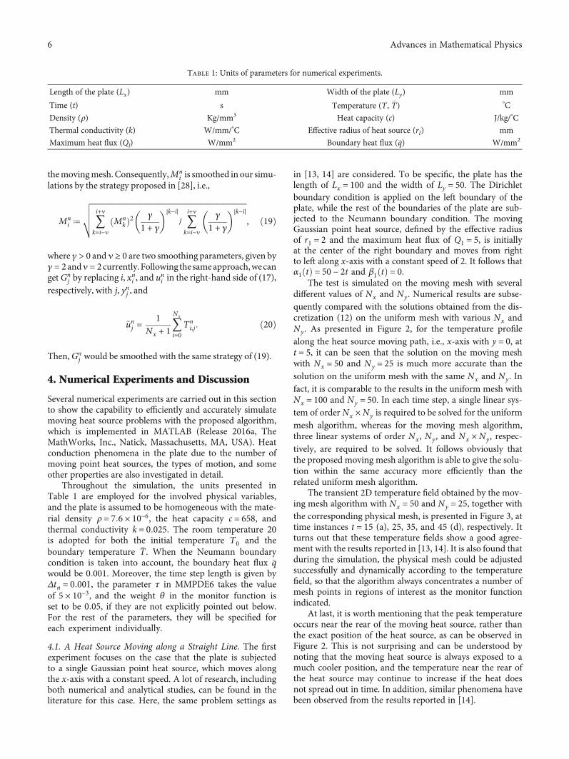
The test is simulated on the moving mesh with severaldifferent values of Nx and Ny . Numerical results are subse-quently compared with the solutions obtained from the dis-cretization (12) on the uniform mesh with various Nx andNy . As presented in Figure 2, for the temperature profilealong the heat source moving path, i.e., x-axis with y = 0, att = 5, it can be seen that the solution on the moving meshwith Nx = 50 and Ny = 25 is much more accurate than thesolution on the uniform mesh with the same Nx and Ny. Infact, it is comparable to the results in the uniform mesh withNx = 100 and Ny = 50. In each time step, a single linear sys-tem of order Nx ×Ny is required to be solved for the uniformmesh algorithm, whereas for the moving mesh algorithm,three linear systems of order Nx , Ny, and Nx ×Ny, respec-tively, are required to be solved. It follows obviously thatthe proposed moving mesh algorithm is able to give the solu-tion within the same accuracy more efficiently than therelated uniform mesh algorithm.

The transient 2D temperature field obtained by the mov-ing mesh algorithm with Nx = 50 and Ny = 25, together withthe corresponding physical mesh, is presented in Figure 3, attime instances t = 15 (a), 25, 35, and 45 (d), respectively. Itturns out that these temperature fields show a good agree-ment with the results reported in [13, 14]. It is also found thatduring the simulation, the physical mesh could be adjustedsuccessfully and dynamically according to the temperaturefield, so that the algorithm always concentrates a number ofmesh points in regions of interest as the monitor functionindicated.

At last, it is worth mentioning that the peak temperatureoccurs near the rear of the moving heat source, rather thanthe exact position of the heat source, as can be observed inFigure 2. This is not surprising and can be understood bynoting that the moving heat source is always exposed to amuch cooler position, and the temperature near the rear ofthe heat source may continue to increase if the heat doesnot spread out in time. In addition, similar phenomena havebeen observed from the results reported in [14].

Table 1: Units of parameters for numerical experiments.

Length of the plate (Lx) mm Width of the plate (Ly) mm

Time (t) s Temperature (T , �T) °C

Density (ρ) Kg/mm3 Heat capacity (c) J/kg/°C

Thermal conductivity (k) W/mm/°C Effective radius of heat source (rl) mm

Maximum heat flux (Ql) W/mm2 Boundary heat flux (�q) W/mm2


–50 –40 –30 –20 –10 0 10 20 30 40 50x

0

100

200

300

400

500

600

700

T

Moving mesh 50⁎25

Uniform mesh 50⁎25





(a)

39 40 41 42 43x

440

460

480

500

520

540

560

580

600

620

T

Moving mesh 50⁎25Uniform mesh 50⁎25Uniform mesh 100⁎50Uniform mesh 200⁎100Uniform mesh 400⁎200Uniform mesh 800⁎400

(b)

47 48 49 50x

325

330

335

340

345

350

355

360

365

370

375

T

Moving mesh 50⁎25Uniform mesh 50⁎25Uniform mesh 100⁎50Uniform mesh 200⁎100Uniform mesh 400⁎200Uniform mesh 800⁎400

(c)

Figure 2: Comparison of temperature profile (a) and their zooms (b, c) along x-axis at t = 5 obtained on the moving mesh with Nx = 50,Ny = 25 and the uniform mesh with various Nx and Ny .


4.2. A Heat Source Moving along a Circle. The second exper-iment considers the case that a square plate with side lengthLx = Ly = 100 is subjected to a single Gaussian point heatsource, which moves along a circle of radius 15 with a con-stant speed in a counterclockwise direction. Specifically,

the heat source has the effective radius of rl = 2 and themaximum heat flux of Ql = 15. Its moving path is set tobe α1ðtÞ = 15 cos ðπt/2Þ and β1ðtÞ = 15 sin ðπt/2Þ. Addi-tionally, all boundaries of the plate are assumed to satisfythe Dirichlet boundary condition.

–50 –10x

–25

–15

–5

5

15

25

y

–50 –30 –10 10–30 3010 50

30 50x

–25

–15

–5

5

15

25

y

100

200

300

400

500

(a)

100

200

300

400

500

–25

–15

–5

5

15

25

y

–50 –30 –10 10 30 50x

–25

–15

–5

5

15

25

y–50 –10

x–30 3010 50

(b)

100

200

300

400

500

–25

–15

–5

5

15

25

y

–50 –30 –10 10 30 50x

–25

–15

–5

5

15

25

y

–50 –10x

–30 3010 50

(c)

100

200

300

400

500

–25

–15

–5

5

15

25

y

–50 –30 –10 10 30 50x

–25

–15

–5

5

15

25

y

–50 –10x

–30 3010 50

(d)

Figure 3: The transient temperature field and the corresponding moving mesh at t = 15 (a), 25, 35, and 45 (d), respectively, for a single heatsource moving along x-axis from right to left.


50

100

150

200

250

300

–50

–30

–10

10

30

50

y

–50 –30 –10 10 30 50x

–50

–30

–10

10

30

50

y

–50 –30 –10 10 30 50x

(a)

50

100

150

200

250

300

–50

–30

–10

10

30

50

y

–50 –30 –10 10 30 50x

–50

–30

–10

10

30

50

y

–50 –30 –10 10 30 50x

(b)

50

100

150

200

250

300

–50

–30

–10

10

30

50

y

–50 –30 –10 10 30 50x

–50

–30

–10

10

30

50

y

–50 –30 –10 10 30 50x

(c)

50

100

150

200

250

350

300

–50

–30

–10

10

30

50

y

–50 –30 –10 10 30 50x

–50

–30

–10

10

30

50

y

–50 –30 –10 10 30 50x

(d)

Figure 4: The transient temperature field and the corresponding moving mesh at t = 1 (a), 2, 3, and 4 (d), respectively, for a single heat sourcemoving along a circle in a counterclockwise direction.


This experiment is simulated by the moving mesh algo-rithm with Nx =Ny = 50 and the weight in the monitorfunction to be θ = 0:2. The transient 2D temperature fieldat time instances t = 1 (a), 2, 3, and 4 (d), respectively, aswell as the corresponding physical mesh, is depicted inFigure 4, where the pink circle represents the heat sourcemoving path. As can be seen from Figure 4, the movingmesh algorithm still successfully concentrates enough meshpoints in regions of interest as the monitor functionindicated.

As a result, the proposed algorithm is also able to beemployed to investigate heat conduction phenomena for thiscase accurately with a small number of Nx and Ny. Thus, agreat improvement in efficiency can be obtained by the pro-posed algorithm.

After a long time simulation, a quasistationary temper-ature field can be achieved. As shown in Figure 5, it wouldbe stationary in the moving coordinate system thatattaches to the moving heat source. Similar results can alsobe found in [29].

4.3. Multiple Heat Sources Moving along Straight Lines. Nowlet us go to investigate the heat conduction phenomena of theplate subjected to multiple moving heat sources. Three cases,that is, two heat sources moving along x-axis in oppositedirections, two heat sources moving along two intersectingstraight lines, and three heat sources moving along threestraight lines parallel to x-axis, are considered below. In allcases, the Dirichlet boundary condition is adopted for the leftboundary of the plate, while the Neumann boundary condi-tion is adopted for the rest of the boundaries of the plate.The all involved heat sources are assumed to be Gaussianpoint heat source with the effective radius to be rl = 2 andthe maximum heat flux to be Ql = 5, except for the last casewhere Ql = 15.

For the first case, the size of the plate is set to be Lx = 200and Ly = 100. The two heat sources are suddenly imposedon the position ð±50, 0Þ, respectively, at the initial time,and then move along x-axis in opposite directions witha constant speed of 2. The resulting moving paths areα1ðtÞ = −α2ðtÞ = −50 + 2t and β1ðtÞ = β2ðtÞ = 0.

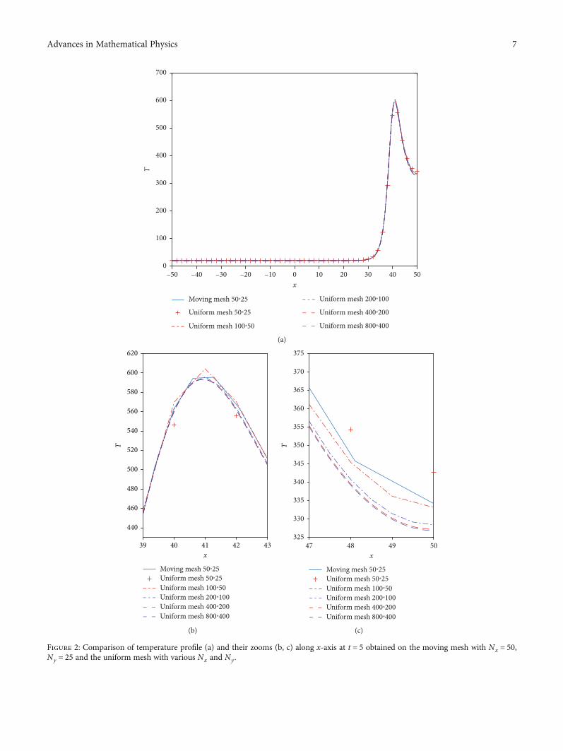
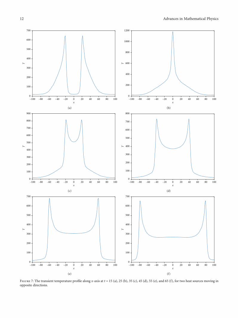
Obviously, the two heat sources will meet each other attime instance t = 25. The simulation is performed by the pro-posed moving mesh algorithm with Nx = 100 and Ny = 50.The corresponding transient 2D temperature field as well asthe physical mesh are presented in Figure 6, for timeinstances t = 15 (a), 25, 35, and 45 (d), respectively. Addition-ally, the 1D temperature profiles along the heat source mov-ing path at time instances t = 15, 25, 35, 45, 55, and 65 aregiven in Figure 7. It can be seen that the physical mesh movesadaptively according to the monitor function of the temper-ature field, in which there exists a peak following each heatsource. As the two heat sources approach each other, twopeaks would merge into a single peak, causing the peak tem-perature to increase rapidly to a high level near 1200. Thentwo peaks are separated as the two heat sources move awayfrom each other, and the peak temperature subsequentlydecreases to the normal level around 650.

For the second case, the plate is square with side lengthLx = Ly = 100. The heat source moving paths are set to be

α1ðtÞ = −α2ðtÞ = β1ðtÞ = β2ðtÞ = −25 +ffiffiffi2

pt. That is, the two

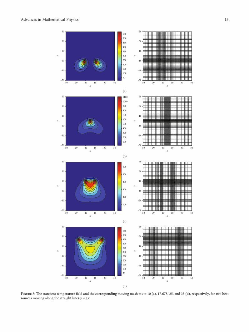
heat sources are initially at the position ð±25,−25Þ, and movealong the straight lines y = ±x, respectively, with the constantspeed of 2. Thus, they will meet each other at the originalpoint ð0, 0Þ at time instance t ≈ 17:678. The transient 2Dtemperature field and the corresponding physical mesh,obtained by the moving mesh algorithm with Nx =Ny = 50,are plotted in Figure 8 for time instances t = 10 (a), 17:678,25, and 35 (d), respectively. Similar phenomena could beobserved as the previous case.

–50

–30

–10

10

30

50

y

200

400

600

800

1000

1200

1400

1600

–50 –10x

–30 3010 50

Figure 5: The quasistationary temperature field for a single heat source moving along a circle in a counterclockwise direction.


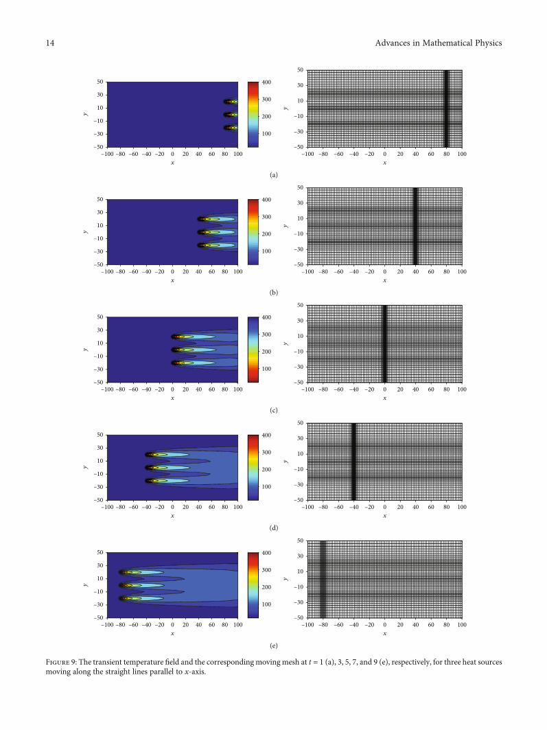
For the last case, the plate is the same as the first case,i.e., Lx = 200 and Ly = 100. The moving paths of the threeheat sources are set to be α1ðtÞ = α2ðtÞ = α3ðtÞ = 100 − 20t,β1ðtÞ = −β3ðtÞ = 20, and β2ðtÞ = 0, which follows that thethree heat sources are initially at the right boundary and

move from right to left along horizontal lines with the sameconstant speed of 20. The resulting transient 2D temperaturefield and the corresponding physical mesh by the movingmesh algorithm with Nx = 100 and Ny = 50 are shown inFigure 9 for time instances t = 1 (a), 3, 5, 7, and 9 (e),

–100 –80 –40 40–60 –20 0 20 60 80 100x

–50

–30

–10

10

30

50

y

–100 –80 –40 40–60 –20 0 20 60 80 100x

–50

–30

–10

10

30

50

y

100

200

300

400

500

600

(a)

200

400

600

800

1000

–100 –80 –40 40–60 –20 0 20 60 80 100x

–50

–30

–10

10

30

50

y

–100 –80 –40 40–60 –20 0 20 60 80 100x

–50

–30

–10

10

30

50

y

(b)

200

400

600

–100 –80 –40 40–60 –20 0 20 60 80 100x

–50

–30

–10

10

30

50

y

–100 –80 –40 40–60 –20 0 20 60 80 100x

–50

–30

–10

10

30

50

y

(c)

100200300400500600

–100 –80 –40 40–60 –20 0 20 60 80 100x

–50

–30

–10

10

30

50

y

–100 –80 –40 40–60 –20 0 20 60 80 100x

–50

–30

–10

10

30

50

y

(d)

Figure 6: The transient temperature field and the corresponding moving mesh at t = 15 (a), 25, 35, and 45 (d), respectively, for two heatsources moving along x-axis in opposite directions.


0

100

200

300

400

500

600

700

T

–100 –80 –40 40–60 –20 0 20 60 80 100x

(a)

0

200

600

400

800

1000

1200

T

–100 –80 –40 40–60 –20 0 20 60 80 100x

(b)

0

100

200

300

400

500

600

900

700

800

T

–100 –80 –40 40–60 –20 0 20 60 80 100x

(c)

0

100

200

300

400

500

600

800

700T

–100 –80 –40 40–60 –20 0 20 60 80 100x

(d)

0

100

200

300

400

500

600

700

T

–100 –80 –40 40–60 –20 0 20 60 80 100x

(e)

0

100

200

300

400

500

600

700

T

–100 –80 –40 40–60 –20 0 20 60 80 100x

(f)

Figure 7: The transient temperature profile along x-axis at t = 15 (a), 25 (b), 35 (c), 45 (d), 55 (e), and 65 (f), for two heat sources moving inopposite directions.


50

100

150

200

250

300

350

400

450

500

550

–50

–30

–10

10

30

50

y

–50 –30 30–10 10 50x

–50

–30

–10

10

30

50

y

–50 –30 30–10 10 50x

(a)

100

200

300

400

500

600

700

800

900

1000

1100

–50

–30

–10

10

30

50

y

–50 –30 30–10 10 50x

–50

–30

–10

10

30

50

y

–50 –30 30–10 10 50x

(b)

100

200

300

400

500

600

–50

–30

–10

10

30

50

y

–50 –30 30–10 10 50x

–50

–30

–10

10

30

50

y

–50 –30 30–10 10 50x

(c)

50

100

150

200

250

300

350

400

450

500

550

–50

–30

–10

10

30

50

y

–50 –30 30–10 10 50x

–50

–30

–10

10

30

50

y

–50 –30 30–10 10 50x

(d)

Figure 8: The transient temperature field and the corresponding moving mesh at t = 10 (a), 17:678, 25, and 35 (d), respectively, for two heatsources moving along the straight lines y = ±x.


100

200

300

400

–100 –80 –40 40–60 –20 0 20 60 80 100x

–50

–30

–10

10

30

50y

–100 –80 –40 40–60 –20 0 20 60 80 100x

–50

–30

–10

10

30

50

y

(a)

100

200

300

400

–100 –80 –40 40–60 –20 0 20 60 80 100x

–50

–30

–10

10

30

50

y

–100 –80 –40 40–60 –20 0 20 60 80 100x

–50

–30

–10

10

30

50

y

(b)

100

200

300

400

–100 –80 –40 40–60 –20 0 20 60 80 100x

–50

–30

–10

10

30

50

y

–100 –80 –40 40–60 –20 0 20 60 80 100x

–50

–30

–10

10

30

50

y

(c)

100

200

300

400

–100 –80 –40 40–60 –20 0 20 60 80 100x

–50

–30

–10

10

30

50

y

–100 –80 –40 40–60 –20 0 20 60 80 100x

–50

–30

–10

10

30

50

y

(d)

100

200

300

400

–100 –80 –40 40–60 –20 0 20 60 80 100x

–50

–30

–10

10

30

50

y

–100 –80 –40 40–60 –20 0 20 60 80 100x

–50

–30

–10

10

30

50

y

(e)

Figure 9: The transient temperature field and the corresponding moving mesh at t = 1 (a), 3, 5, 7, and 9 (e), respectively, for three heat sourcesmoving along the straight lines parallel to x-axis.


respectively. Again, the physical mesh could be adjusted suc-cessfully according to the monitor function of the tempera-ture field. Since the heat sources move much faster thanother cases, the peak temperature in this case is smaller thanthe one in the previous cases.

5. Conclusions

A simple moving mesh algorithm has been developed tonumerically solve the 2D model equations of moving heatsource problems with Gaussian point heat sources. In thepresent algorithm, only two additional 1D mesh equationsare required to be solved for each time step. However, it isfound that the physical mesh could successfully and dynam-ically concentrate a number of mesh points in regions ofinterest as the monitor function indicated. Therefore, theproposed algorithm is able to simulate the moving heatsource problem very accurately and efficiently. Heat conduc-tion phenomena of the rectangular plate subjected to movingGaussian point heat sources with various types of motion,including moving along straight lines and a circular trajec-tory, have then been numerically investigated. Numericalresults validate the accuracy and efficiency of the proposedalgorithm, which shows that the proposed moving meshalgorithm is a promising approach for such moving heatsource problems.

Finally, the extension of the proposed moving mesh algo-rithm to other localized heat source models, such as Diracdelta point heat source and plane heat source, is ongoingand would be presented elsewhere soon. The full 3D simula-tion of the moving heat source problem with the movingmesh method will also be studied in the future work.

Data Availability

The data used to support the findings of this study areincluded within the article.

Conflicts of Interest

The authors declare that there are no conflicts of interestregarding the publication of this paper.

Acknowledgments

The authors would like to express their sincere appreciationto the editor and the anonymous referees for their valuablecomments and suggestions. This work was supported bythe National Natural Science Foundation of China (grantnumber 11601229) and the Jiangsu Province Natural ScienceFoundation of China (grant number BK20160784).

References

[1] D. W. Hahn and M. N. Özişik, “Moving heat source problems,”in Heat Conduction, chapter 11, pp. 433–451, John Wiley &Sons, Inc., Hoboken, 3rd edition, 2012.

[2] A. J. Panas, “Moving heat sources,” in Encyclopedia of ThermalStresses, chapter 688, pp. 3215–3227, Springer Science+Busi-ness Media, LLC, Dordrecht, 2014.

[3] S. B. Powar, P. M. Patane, and S. L. Deshmukh, “A reviewpaper on numerical simulation of moving heat source,” Inter-national Journal of Current Engineering and Technology, vol. 4,pp. 63–66, 2016.

[4] V. Zdeněk, H. Milan, and M. Jiří, “3Dmodel of laser treatmentby a moving heat source with general distribution of energy inthe beam,” Applied Optics, vol. 55, no. 34, pp. D140–D150,2016.

[5] M. Pamuk, A. Savaş, Ö. Seçgin, and E. Arda, “Numerical sim-ulation of transient heat transfer in friction-stir welding,”International Journal of Heat and Technology, vol. 36, no. 1,pp. 26–30, 2018.

[6] K. He, Q. Yang, D. Xiao, and X. Li, “Analysis of thermo-elasticfracture problem during aluminium alloy MIG welding usingthe extended finite element method,” Applied Sciences, vol. 7,no. 1, p. 69, 2017.

[7] Y. Sun, S. Liu, Z. Rao, Y. Li, and J. Yang, “Thermodynamicresponse of beams on Winkler foundation irradiated by mov-ing laser pulses,” Symmetry, vol. 10, no. 8, p. 328, 2018.

[8] E. Mirkoohi, J. Ning, P. Bocchini, O. Fergani, K.-N. Chiang,and S. Y. Liang, “Thermal modeling of temperature distribu-tion in metal additive manufacturing considering effects ofbuild layers, latent heat, and temperature-sensitivity of mate-rial properties,” Journal of Manufacturing and Materials Pro-cessing, vol. 2, no. 3, p. 63, 2018.

[9] E. Mirkoohi, D. E. Seivers, H. Garmestani, and S. Y. Liang,“Heat source modeling in selective laser melting,” Materials,vol. 12, no. 13, p. 2052, 2019.

[10] P. Bian, X. Shao, and J. Du, “Finite element analysis of thermalstress and thermal deformation in typical part during SLM,”Applied Sciences, vol. 9, no. 11, p. 2231, 2019.

[11] D. Rosenthal, “Mathematical theory of heat distribution dur-ing welding and cutting,” Welding Journal, vol. 20, pp. 220–234, 1941.

[12] J. Ma, Y. Sun, and J. Yang, “Analytical solution of dual-phase-lag heat conduction in a finite medium subjected to a movingheat source,” International Journal of Thermal Sciences,vol. 125, pp. 34–43, 2018.

[13] X.-T. Pham, “Two-dimensional Rosenthal moving heat sourceanalysis using the meshless element free Galerkin method,”Numerical Heat Transfer, Part A: Applications, vol. 63,no. 11, pp. 807–823, 2013.

[14] E. O. Reséndiz-Flores and F. R. Saucedo-Zendejo, “Two-dimensional numerical simulation of heat transfer with mov-ing heat source in welding using the finite pointset method,”International Journal of Heat and Mass Transfer, vol. 90,pp. 239–245, 2015.

[15] J. Winczek, “The influence of the heat source model selectionon mapping of heat affected zones during surfacing by weld-ing,” Journal of Applied Mathematics and ComputationalMechanics, vol. 15, no. 3, pp. 167–178, 2016.

[16] M. Akbari, D. Sinton, andM. Bahrami, “Geometrical effects onthe temperature distribution in a half-space due to a movingheat source,” Journal of Heat Transfer, vol. 133, no. 6, article064502, 2011.

[17] W. Huang and R. D. Russell, Adaptive Moving Mesh Methods,Springer Science+Business Media, LLC, New York, 2011.

[18] C. J. Budd, W. Huang, and R. D. Russell, “Adaptivity withmoving grids,” Acta Numerica, vol. 18, pp. 111–241, 2009.

[19] K. Liang, P. Lin, M. T. Ong, and R. C. E. Tan, “A splittingmoving mesh method for reaction-diffusion equations of


quenching type,” Journal of Computational Physics, vol. 215,no. 2, pp. 757–777, 2006.

[20] Z. Hu and H. Wang, “A moving mesh method for kinetic/hy-drodynamic coupling,” Advances in Applied Mathematics andMechanics, vol. 4, no. 6, pp. 685–702, 2012.

[21] Q. Gao and S. Zhang, “Moving mesh strategies of adaptivemethods for solving nonlinear partial differential equations,”Algorithms, vol. 9, no. 4, p. 86, 2016.

[22] W. Huang, Y. Ren, and R. D. Russell, “Moving mesh partialdifferential equations (MMPDES) based on the equidistribu-tion principle,” SIAM Journal on Numerical Analysis, vol. 31,no. 3, pp. 709–730, 1994.

[23] W. Huang, “An introduction to MMPDElab,” 2019, http://arxiv.org/abs/1904.05535.

[24] W. Huang and L. Kamenski, “On the mesh nonsingularity ofthe movingmesh PDEmethod,”Mathematics of Computation,vol. 87, no. 312, pp. 1887–1911, 2018.

[25] J. Ma and Y. Jiang, “Moving mesh methods for blowup inreaction-diffusion equations with traveling heat source,” Jour-nal of Computational Physics, vol. 228, no. 18, pp. 6977–6990,2009.

[26] Z. Hu, “Numerical investigation of heat conduction with mul-tiple moving heat sources,” Symmetry, vol. 10, no. 12, p. 673,2018.

[27] M. A. Beauregard and Q. Sheng, “An adaptive splittingapproach for the quenching solution of reaction-diffusionequations over nonuniform grids,” Journal of Computationaland Applied Mathematics, vol. 241, pp. 30–44, 2013.

[28] W. Huang, Y. Ren, and R. D. Russell, “Moving mesh methodsbased on moving mesh partial differential equations,” Journalof Computational Physics, vol. 113, no. 2, pp. 279–290, 1994.

[29] J. Kidawa-Kukla, “Temperature distribution in a rectangularplate heated by a moving heat source,” International Journalof Heat and Mass Transfer, vol. 51, no. 3-4, pp. 865–872, 2008.


http://arxiv.org/abs/1904.05535

http://arxiv.org/abs/1904.05535

heat conduction simulation of 2d moving heat source...

Documents