heat and mass transfer in convective drying...

*Technical University of Civil Engineering Bucharesthttp://www.utcb.ro

Heat and Mass Transfer in Heat and Mass Transfer in Convective Drying Convective Drying

ProcessesProcesses

Camelia GAVRILA* Adrian Gabriel GHIAUS*

Ion GRUIA**

**University of Bucharesthttp://www.unibuc.ro

Presented at the COMSOL Conference 2008 Hannover

• Introduction

• Mathematical modelling of drying processes

• Modelling Results

• Conclusions

CONTENTCONTENT

Transport Phenomena5.11. 2008 2 / 18

• AIM: describe the modelling and simulation of the dehydration

of fruits and vegetables (grapes) in a complex drying system

processes, using COMSOL Multiphysics Program

– simulation of unsteady convective drying of grapes in static bed

conditions

• USE of a dynamic mathematical model, based on

– physical and transport properties

– mass and energy balances.

INTRODUCTIONINTRODUCTION


The simulation of various product drying systems involves

solving a set of heat and mass transfer equations which

describe:

• heat and moisture exchange between product and air,

• adsorption and desorption rates of heat and moisture

transfer,

• equilibrium relations between product and air,

• psychometrics properties of moist air.

Mathematical modellingMathematical modellingEquation typesEquation types


• The most rigorous methods of describing the drying process are derived from the concepts of irreversible thermodynamics in which the various fluxes are taken to be directly proportional to the appropriate “potential”, (Ghiaus, 1997).

Mathematical modellingMathematical modellingGeneral Ideas General Ideas -- 11




• For most engineering heat transfer calculations performed in

commercial food dehydration, accuracy greater than 2-5 % is

seldom needed.

• This is because errors due to varying or inaccurately

measured boundary conditions such as air temperature and

velocity, would overshadow errors caused by inaccurate

thermal properties.



• Most thermal property models are empirical rather than

theoretical

- they are based on statistical curve fitting rather than

theoretical derivations involving heat transfer analysis

• The water is treated as a single, uniform component of the

food product. It could be argued that the thermal properties of

water in the food depend on how it is configured or “bound”

within the product.

Where

XX - grape moisture content;

T T - the air temperature;

ρρb b - bulk bed density;

c c - specific heat capacity;

λλ - thermal conductivity;

DDeffeff - effective mass diffusivity.

Mathematical modellingMathematical modellingEquationsEquations


The mass balance inside the product can be written as:

and the heat-energy balance can be set down as

( )∂ ρ∂

ρ∂∂

bb eff

Xt

div DXz

⋅= ⋅ ⋅⎛

⎝⎜⎞⎠⎟

ρ∂∂

λ∂∂b c

Tt

divTz

⋅ ⋅ = ⋅⎛⎝⎜

⎞⎠⎟

Mathematical modellingMathematical modellingParameters for Corinthian grapesParameters for Corinthian grapes


691Bulk bed density, ρb [kg/m3]

3.6·10-9Effective diffusion, Deff, [m2/s]

3600Specific heat, c, [J/kg K]

0.5721Thermal conductivity, λ, [W/m K]

75Water content, W, [%]

ValueItem

Results and DiscussionResults and Discussion


• COMSOL Mutiphysics program is used to simulate the

dehydration of grapes in a complex drying system

processes which correspond to the numerical solution of

these model equations.

• The above system of non-linear Partial Differential

Equations, together with the already described set of initial

and boundary conditions, has been solved by Finite

Elements Method implemented by Comsol Multiphysics 3.4.

Results and DiscussionResults and Discussion


• Steps:

- Build the geometry of the

model,

-Fix the boundary settings,

the mesh parameters

-Fix the Parameters for

Corinthian grapes

- Compute the final solution.Results from the compute solution in COMSOL Multiphysics

Results and DiscussionResults and DiscussionTemperatureTemperature


• Evolution of grape temperature during the drying process, at the surface and bottom of the bed and as an average. • Differences of temperature between the base and surface of the bed appear only during the first period of drying, approx. the first 5 hours. After this the bed temperature remains uniform Evolution of grape temperature during

the drying process.

0 5 10 15 20 25 30 35

25

30

35

40

surface of grape bed average bottom of grape bed

Tem

pera

ture

, oC

Time, h

Results and DiscussionResults and DiscussionMoistureMoisture


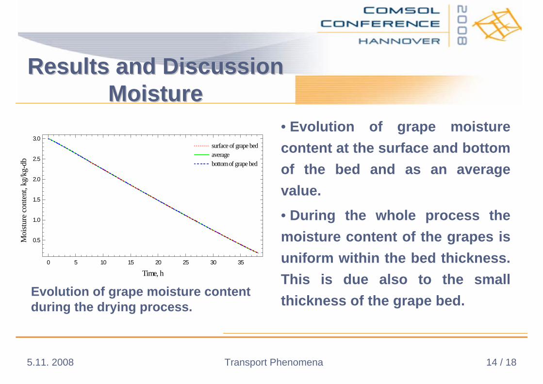
• Evolution of grape moisture content at the surface and bottom of the bed and as an average value.

• During the whole process the moisture content of the grapes is uniform within the bed thickness. This is due also to the small thickness of the grape bed.Evolution of grape moisture content

during the drying process.

0 5 10 15 20 25 30 35

0.5

1.0

1.5

2.0

2.5

3.0 surface of grape bed average bottom of grape bed

Moi

sture

con

tent

, kg/

kg-d

b

Time, h

Results and DiscussionResults and DiscussionDrying RateDrying Rate


• Parameter: drying rate- Represents the rate of evaporated water from one square meter of drying product.

• At the beginning of the process it increases from 0.06 g/s m2 to 0.12 g/s m2 and then has a very small decreasing slope.

• At the end of the process it decreases rapidly.

Drying rate vs. drying time for grape dehydration.

0 5 10 15 20 25 30 35

0.06

0.07

0.08

0.09

0.10

0.11

0.12

0.13

0.14

Dry

ing

rate

, g/s

m2

Time, h

Results and DiscussionResults and DiscussionDDryingrying AAirir TTemperatureemperature


Drying air temperature at different locations vs. drying time.

0 5 10 15 20 25 30 35

25

30

35

40

45

50

55

60

65

70

preheated exhaust ambient

inlet drying room outlet drying room inlet heat exchanger

Tem

pera

ture

, oC

Time, h

Results and DiscussionResults and DiscussionRRelative elative HHumidityumidity


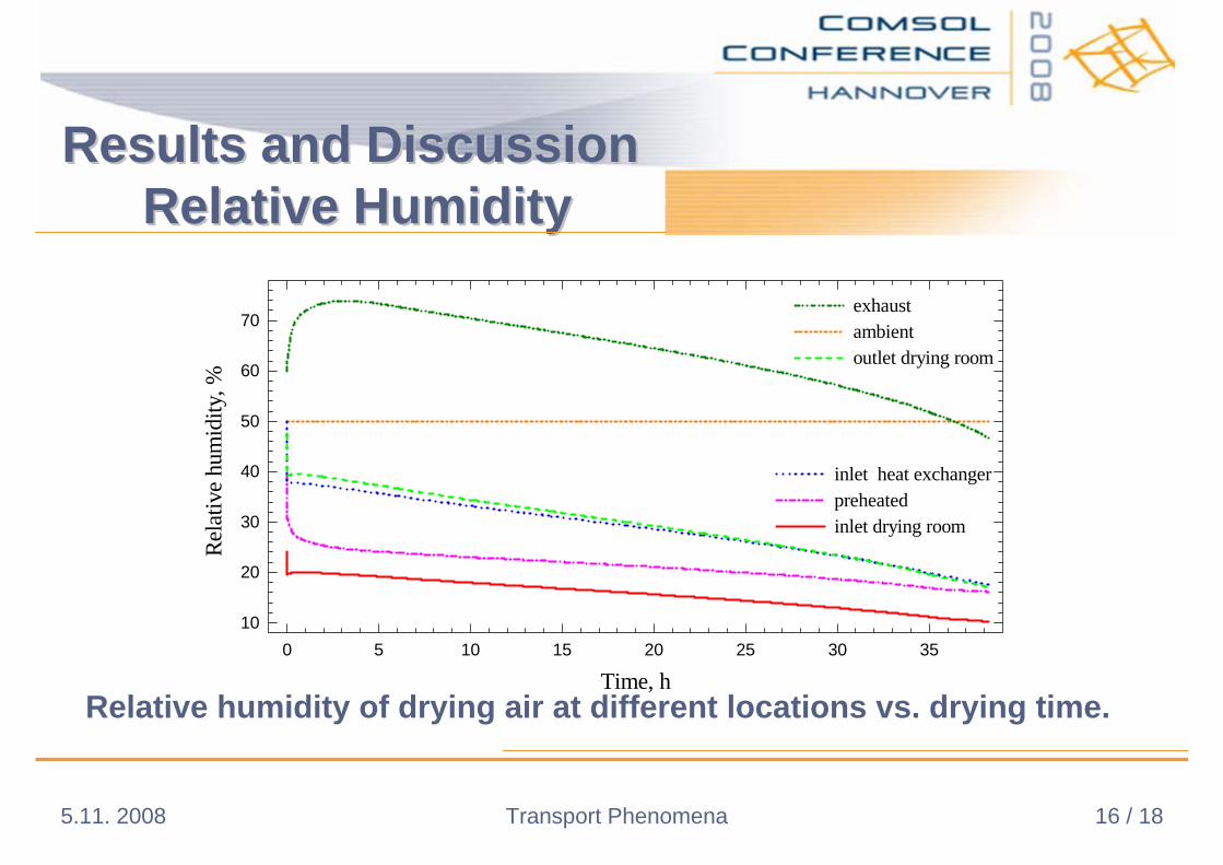
Relative humidity of drying air at different locations vs. drying time.

0 5 10 15 20 25 30 3510

20

30

40

50

60

70

inlet heat exchanger preheated inlet drying room

exhaust ambient outlet drying room

Rela

tive

hum

idity

, %

Time, h

CONCLUSIONSCONCLUSIONS


• We have demonstrated the versatility of COMSOL

Multiphysics with regard to the modelling and simulation of

the dehydration of grapes in a complex drying system

processes.

•The model was applied to the full scale experimental data

with good results.

*Technical University of Civil Engineering Bucharesthttp://www.utcb.ro

Camelia GAVRILA* [email protected] Gabriel GHIAUS* [email protected] GRUIA** [email protected]

**University of Bucharesthttp://www.unibuc.ro

Thank You!

heat and mass transfer in convective drying...

Documents