heart rate variability acquisition from ambulatory

Escola Tècnica Superior d’Enginyeria de Telecomunicació de BarcelonaGrau en Enginyeria Física

Treball Final del Grau en Enginyeria Física

Heart rate variability acquisition fromambulatory measurements of IPG

Ricard Cuervo Saliné

Thesis Director Jaime Oscar Casas PiedrafitaInstrumentation, Sensors and Interfaces GroupUniversitat Politècnica de Catalunya

June 22, 2017

Ricard Cuervo Saliné

Heart rate variability acquisition from

ambulatory measurements of IPG

June 22, 2017

Thesis Director: Jaime Oscar Casas Piedrafita

Universitat Politècnica de Catalunya

Grau en Enginyeria Física

Escola Tècnica Superior d’Enginyeria de Telecomunicació de Barcelona

C/Jordi Girona, 1

08034 and Barcelona

Abstract

Stress plays a vital role in the declaration of certain illnesses, it depresses the immunesystem and can led to the worsening of some conditions. It is therefore of utmostimportance to have a reliable tool capable of monitoring stress levels with regularity(hence, in ambulatory scenarios) and without representing a hassle (hence, withease of use, embedded in some common objects).

The main objective of this work is to present a suitable set-up capable of retrievingstress measures. For this purpose the electrocardiogram (ECG) and the impedancepletysmography (IPG) signals have been acquired and processed. The impedancesignal has been studied and characterized as a suitable alternative to replace ECG insituations where the latter can not be acquired with sufficient quality. Furthermorethe ECG has also been improved thanks to the IPG, the electrical signal has beenrecovered from noisy recordings thanks to the implementation of a filter and byusing the impedance signal increasing in this manner its capabilities.

The autonomic nervous system regulates among others the heart rate (HR) and isrelated with the fight or flight response trough the sympathetic system and to therecovery after the exposure to a stressor trough the vagal system. The study of heartrate variability (HRV) has proved to detect the activity of both systems providing anon invasive tool for stress measurements.

A thorough study of the HRV and its relation with stress is carried out in this work,studying the effect of different tests as well as the influence of breath rate. All resultshave ultimately been used to assure the feasibility of IPG as a source of reliableinformation when retrieving stress levels and hence proving the potential use of thissignal to new devices.

iii

Acknowledgement

This project would have never seen the light of day without the guidance of Prof.Oscar Casas. His was the original idea for this work and has been helping everyday since the beginning, not only allowing me to progress and accomplish the goalsbut also making sure I understood the concepts. I would like to thank him for theadditional effort he put in the educational part of this work and for his infinitepatience when resolving my doubts an questions (which were quite a few).

Additionally I am also thankful to him, as well as the rest of the people form ISIgroup for making me feel welcome. Also for sharing opinions with me that werealways enriching and led me to investigate further and with major detail someaspects of my work. Finally, for helping with the measurements by submitting to mytests and providing the necessary recordings for this project.

I’m also gratefully to my friends and family with whom I shared the best and theworst of this last years and without whom I would not be who I am today. Theyhave withstood with me the difficulties which I faced and allowed me to grow as aperson.

iv

Contents

1 Introduction 11.1 Motivation and Problem Statement . . . . . . . . . . . . . . . . . . . 1

1.1.1 Stress . . . . . . . . . . . . . . . . . . . . . . . . . . . . . . . 11.1.2 The Autonomic Nervous System . . . . . . . . . . . . . . . . . 2

1.2 Current technologies and research . . . . . . . . . . . . . . . . . . . 31.3 Objectives . . . . . . . . . . . . . . . . . . . . . . . . . . . . . . . . . 41.4 Thesis approach . . . . . . . . . . . . . . . . . . . . . . . . . . . . . . 61.5 Thesis Structure . . . . . . . . . . . . . . . . . . . . . . . . . . . . . . 6

2 Theoretical foundations 82.1 Biological background . . . . . . . . . . . . . . . . . . . . . . . . . . 8

2.1.1 The heart and the heartbeat . . . . . . . . . . . . . . . . . . . 82.2 The electrocardiogram (ECG) . . . . . . . . . . . . . . . . . . . . . . 9

2.2.1 The heart dipole model . . . . . . . . . . . . . . . . . . . . . 92.2.2 The ECG wave . . . . . . . . . . . . . . . . . . . . . . . . . . 10

2.3 The IPG signal . . . . . . . . . . . . . . . . . . . . . . . . . . . . . . 112.3.1 The model . . . . . . . . . . . . . . . . . . . . . . . . . . . . . 13

2.4 Mathematical tools . . . . . . . . . . . . . . . . . . . . . . . . . . . . 142.4.1 AM demodulation . . . . . . . . . . . . . . . . . . . . . . . . 142.4.2 Time-frequency analysis . . . . . . . . . . . . . . . . . . . . . 162.4.3 Adaptive filtering . . . . . . . . . . . . . . . . . . . . . . . . . 18

3 Hardware development 213.1 General overview . . . . . . . . . . . . . . . . . . . . . . . . . . . . . 213.2 The ECG acquisition system . . . . . . . . . . . . . . . . . . . . . . . 223.3 The IPG acquisition system . . . . . . . . . . . . . . . . . . . . . . . . 24

3.3.1 The current source . . . . . . . . . . . . . . . . . . . . . . . . 243.3.2 The acquisition circuit . . . . . . . . . . . . . . . . . . . . . . 25

4 Software development 284.1 The Pan Tompkins algorithm . . . . . . . . . . . . . . . . . . . . . . . 284.2 Signal filtering . . . . . . . . . . . . . . . . . . . . . . . . . . . . . . 324.3 Breath rate demodulation . . . . . . . . . . . . . . . . . . . . . . . . 334.4 Stress measures . . . . . . . . . . . . . . . . . . . . . . . . . . . . . . 34

v

4.4.1 The tests . . . . . . . . . . . . . . . . . . . . . . . . . . . . . . 344.4.2 Processing the recordings . . . . . . . . . . . . . . . . . . . . 35

5 Results and discussion 375.1 Tachogram . . . . . . . . . . . . . . . . . . . . . . . . . . . . . . . . 375.2 Breath rate . . . . . . . . . . . . . . . . . . . . . . . . . . . . . . . . 385.3 Stress measurements . . . . . . . . . . . . . . . . . . . . . . . . . . . 395.4 Further study of IPG signals . . . . . . . . . . . . . . . . . . . . . . . 405.5 Filtering of the ECG . . . . . . . . . . . . . . . . . . . . . . . . . . . . 42

6 Conclusions 456.1 The IPG and the HR . . . . . . . . . . . . . . . . . . . . . . . . . . . 456.2 Breath effect . . . . . . . . . . . . . . . . . . . . . . . . . . . . . . . 466.3 Stress . . . . . . . . . . . . . . . . . . . . . . . . . . . . . . . . . . . 466.4 IPG variability; an alternative to HF analysis? . . . . . . . . . . . . . 476.5 Adaptive filter . . . . . . . . . . . . . . . . . . . . . . . . . . . . . . . 486.6 Future Work and perspectives . . . . . . . . . . . . . . . . . . . . . . 49

Bibliography 51

Acronyms 56

Appendices 58

A Codes 58A.1 Python codes . . . . . . . . . . . . . . . . . . . . . . . . . . . . . . . 58

A.1.1 Real time Pan Tompkins algorithm . . . . . . . . . . . . . . . 58A.1.2 Stroop test implementation . . . . . . . . . . . . . . . . . . . 64

A.2 Matlab codes . . . . . . . . . . . . . . . . . . . . . . . . . . . . . . . 74A.2.1 ECG Pan Tompkins algorithm . . . . . . . . . . . . . . . . . . 74A.2.2 IPG Pan Tompkins algorithm . . . . . . . . . . . . . . . . . . . 76A.2.3 RR interval check . . . . . . . . . . . . . . . . . . . . . . . . . 78A.2.4 IPNLMS filter function . . . . . . . . . . . . . . . . . . . . . . 79A.2.5 Frequency analysis for stress detection . . . . . . . . . . . . . 80

vi

1Introduction

„Wisdom comes from experience. Experience isoften a result of lack of wisdom.

— Terry Pratchett

1.1 Motivation and Problem Statement

The study of physiological signals provides a huge amount of information about thehealth state of a subject. Those biosignals can be obtained in ambulatory scenarios bymeans of different devices, the vast majority of which have a relative low price. Thisprovides a tool capable of performing regular, non invasive cheap controls in patientsin order to control several conditions and, thus, prevent any complications.

Heart rate related biosignals can provide, among others, information about heartdiseases before they manifest. It is of the utmost importance to be able to retrievethose signals efficiently and also to interpret and extract the information enclosedwithin.

1.1.1 Stress

The importance of stress

A link between acute or prolonged stress episodes and the development of severalillnesses has been found in the past years. Chronic stress increases the risk ofsuffering from mental and physical health problems such as depression and anxietyor ischemic heart disease. It can also result in several problems derived from thedepression of the immune system, patients with higher stress levels have been foundto be more likely to contract common cold virus. In addition patients with HIV whosuffered from higher cumulative levels of stress showed a faster progression towardsAIDS [1].

1

In addition stress detection could also help give voice to those who can not speakby their own. People who suffer from autism, cerebral paralysis or other kindsof disabilities can not always express their level of comfort or wellness. A devicecapable of measuring stress levels on the flight has the potential to indicate whenthose people are not comfortable with its environment. Autistic people adapting to anew situation or surroundings are an example of this possible application.

A reliable and cost-effective method, capable of monitoring stress levels in homeenvironments would allow for an early detection of stress and, therefore, couldincrease the quality of life and prevent future complications mentioned above. As aresult health care expenses derived from the treatment of those complications wouldalso reduce.

Physiology of stress

Physiological stress is the response of the body to a challenge or stressor, an alterationin its environment that triggers a reaction in multiple body systems. Here, thedefinition of stress as the mismatch between perceived demands and perceivedcapacities to meet those demands is used[2]. This mismatch alters amongst othersthe autonomic nervous system (ANS) which responds by increasing the activationof the sympathetic system as it will be explained in section 1.1.2. This responseultimately results in an increased heart rate (HR) and breath rate and its known asthe fight or flight response [3]. When the stressor disappears the vagal branch of theANS takes over reducing the HR.

Heart rate variability (HRV) accounts for the variation in the duration of heartbeats.The study of HRV provides information about the increasing or decreasing HR overtime and, thus, information about the balance in the ANS which can be related tostress [2]. The study of HRV is therefore a non-invasive technique that allows forthe detection and study of stress. Since HR can be obtained in ambulatory scenariosfrom a variety of cost-effective devices, this method also allows for a regular, athome monitoring of patients.

1.1.2 The Autonomic Nervous System

The Autonomic Nervous System (ANS) belongs to the Peripheral nervous system(PNS) and contains the efferent pathways which connects controlling centres inthe brain to effector organs other than skeletal muscle. Consequently, heart ratevariability is linked to the effect of the ANS. The ANS is divided anatomically intothe sympathetic and parasympathetic (or vagal) systems. Both systems are involvedin the modulation of heart rate having opposing effects.

1.1 Motivation and Problem Statement 2

The vagal system regulates responses related with the maintenance and conservationof the body function, thus, actions such as the slowing of the heart rate or theconstriction of the pupils are mediated by an activation of the vagal system.

The sympathetic system is more related with what is known as the "fight or flight"response [3] and, therefore, related with stress response. An activation of thesympathetic system results in a number of effects such as increasing of the heartrate, pupillary dilation, decreased muscle fatigue or elevated blood glucose [2].

The activity of tissues that are controlled by both systems depends on the balancebetween the two, however one of them is usually dominant. Hence the diameter ofthe pupils or the resting heart rate depends mainly on the vagal tone (i.e. the levelof activity of the parasympathetic system). Changes in the activity of the tissues arethe result of the combination of both systems activity.

1.2 Current technologies and research

Nowadays there exists many devices capable of sensing the electrocardiogram (ECG)signal available in the market. Those devices allow some minor distortion of thesignal as they are fitted for ambulatory scenarios and they also suppress the need foran electrolytic gel usually employed in clinical scenarios. The use of dry electrodesavoid the nuisance while yielding sufficiently good results, their main drawbacks aretheir increased settling time after an artifact takes place and its greater impedance.One of the main drawbacks of ECG measures is the need to place the electrodesfar away from each other. In order to get an accurate measurement electrodes areusually placed on opposite limbs which is annoying and inconvenient.

The ECG signal has also been widely studied in the literature, methods to obtaina great amount of information had been proposed and tested. The harvesting andprocessing of HR has improved over the years and there exist reliable methods forthat purpose. The ECG can also retrieve the breath rate and there exists a number ofways of doing so [4–9]. Stress measurements can be derived from the sympathovagalbalance which is calculated trough the HRV, many studies [10–15] use this techniqueas it is a non invasive one although some inconsistencies has been found in theliterature.

Needless to say ECG has a vital role in cardiac diseases diagnostics and it’s usedworldwide to study the healthiness of the heart. ECG can detect abnormal func-tioning of the heart such as arrhythmias, myocardial infarction or enlarged heart.

1.2 Current technologies and research 3

Moreover, the study of HRV has also been proved useful in premature diagnosis ofmyocardial infarction and diabetes neuropathy

Photopletysmogram (PPG) is another widely used signal to detect and control thepressure pulse of the cardiac cycle. It is based on the detection of changes in bloodvolume of a certain region by means of light absorption. There exist currently manydevices oriented to retrieve the PPG pressure-pulse signal in clinical scenarios wherethe acquisition can be controlled and there are fewer artifacts. Also PPG is used insome ambulatory applications such as wrist acquisition of the pulse (implementedin watches) however the measurements suffer greatly from motion artifacts. Thesensor must be also applied over an artery and is sensible to the pressure appliedover the skin.

IPG signal is relatively unexplored due to the widespread popularity of the photo-pletysmogram (PPG) signal, which provides about the same information relative topulse-pressure waveforms. However, IPG is somewhat more versatile as it allowsmeasurements from limb to limb as well as measurements along a single vessel.Since IPG is a mostly unexplored technique there are very few commercial deviceswhich use this method. Some weighing scales use IPG to retrieve the blood pulsesignal at the foot [16].

There exist very few information about the IPG signal as a result of its lack of use.Many procedures that retrieve information such as the breath rate or the HR haveonly been develop and studied for PPG or ECG signals, due to the similarities withPPG it is reasonable to assume those procedures to be implementable to IPG in arelatively straightforward manner.

1.3 Objectives

The usefulness of the retrieving, processing and study of cardiac signals has beenalready described. The aim of this work must therefore be separated into two distinctsections.

The first goal should be the understanding of the underlying biological processesas well as well as a comprehension of the underlying mechanism that allows forthe acquisition. This knowledge would then be required during the building of afunctional acquisition hardware set-up. The developed hardware must be able toacquire good quality ECG and IPG signals in ambulatory scenarios while requiring alow cost for its building and a low voltage for its powering. The set-up should onlyneed four electrodes as IPG acquisition systems need two pairs, one pair for injecting

1.3 Objectives 4

current and the other pair for measuring voltage differences, the later can howeverbe re-purposed for measuring the ECG signal simultaneously.

Once the signals have been acquired the goal should be obtaining as much informa-tion from them as possible. Stress measurements will be on the spotlight as theyrepresent a huge interest and have great potential and usefulness. A set of softwaretools must be implemented, those programs must be able to extract the requiredinformation and present it in a way the user can clearly distinguish between stressor relaxation periods.

The acquisition of a quality ECG signal is not possible everywhere in the body.The presence of electromyogram (EMG), another electrical signal derived from themuscular activity, may contaminate the measurements. It is specially present infoot-to foot measures where the contamination may hide entirely the signal and cannot be suppressed by means of a bandpass filter.

A procedure for suppressing EMG contamination wold be of great use, as the mea-surements are done in distal sites, specially from limb to limb, muscular activity hasa major influence in our measurements and can potentially mask the desired signal.Therefore, the study and implementation of a way to suppress EMG informationfrom the signal will be carried on. Respiration has great influence in hearth rate andis also greatly affected during periods of stress. It is important to ensure there is nodirect influence of breath rate on the stress measurements derived from the study ofHRV. To do so the breath rate information would be extracted from the signals andcompared to the retrieved information.

IPG signals present some unique advantages that could make them a more suitableoption for retrieving the previously mentioned information. They are easier andcheaper to obtain that its PPG counterparts as they can be implemented by means ofelectrodes and the impedance measurements does not require the precise placementthat optical measurements need. When compared to the ECG signal, IPG has anarrower frequency bandwidth, this allows for a more aggressive filtering of thesignal which reduces or even eliminates the contamination produced by EMG, aclean IPG signal can be obtained from foot-to-foot without any additional effort.

Being able to obtain the same parameters listed above from the IPG signal wouldrepresent a major advantage in many situations. To ensure the reliability of theresults a study should be carried out. Its main objective will be to clarify whetheror not the HR can be derived from the pressure-pulse signal and, therefore, if allthe derived information can be obtained from it. A positive result will open thepossibility for the extraction of all kinds of informations from IPG which will increasegreatly the number of potential uses.

1.3 Objectives 5

1.4 Thesis approach

To understand and act over every step from the acquisition of the signals to their finalprocessing and harvesting of the desired information it is necessary to work at severallevels simultaneously. Building the hardware and simultaneously implementing thesoftware that processes the signal allows for a deeper understanding and insight ofthe whole process. It would also permit to apply the necessary modifications at alllevels.

Another goal set for this project is to prove the feasibility of a stress detecting devicewith the developed techniques, the final device should be small or at least mobileand the information should be delivered without further delay trough an screen suchas the one of a mobile phone.

The complete set-up would integrate all the parts. The sensing circuits shouldbe connected to an analog to digital (AD) converter capable of transferring theinformation for its later processing. An ideal way of sending the information wouldbe via bluetooth or some other wireless technology as this allows for a greaterflexibility in the final set-up. The data should then be retrieved and processed by aprocessing core powerful enough to perform fast complex mathematical operations(such as Fourier transforms or integrators) whilst being small enough to move aroundand not be a hassle. Another criteria to consider is that the processing core hasa compatible channel of communication with the AD allowing both to send andretrieve the data. Finally the results need to be shown in some screen whether it isone connected to the processing core, from a computer or even from a mobile phonefor maximum versatility.

1.5 Thesis Structure

Chapter 2

This chapter is dedicated to develop in a comprehensive way the theoretical founda-tions required to understand the procedures and results later on presented in thisdocument. An overview of the main biological concepts involved in the detection ofHR is carried out. Also the main mathematical tools used during the data analysisare presented here.

Chapter 3

This chapter presents the development process of the hardware. the design criteria

1.4 Thesis approach 6

and the specifications are explained with detail. The final set-up is also shownalongside with its characterization ans the retrieved output is shown.

Chapter 4

This chapter presents all the tools used during the signals processing. The mainalgorithms are explained as well as the decision criteria to choose one platform orother. The evolution of the data processing and the necessity to develop the suitabletools required to retrieve all the desired information are presented here.

Chapter 5

This chapter shows the obtained results alongside with examples of the signal andthe derived information. The results are illustrated and put in context, relatingone test with another to connect all tests an its results. A summary of the mainobservations made during the development of this work is done here.

Chapter 6

This chapter discusses the results obtained and its main implications. In this chapterall the retrieved information is discussed and several hypothesis about the observedresults are presented.

1.5 Thesis Structure 7

2Theoretical foundations

2.1 Biological background

2.1.1 The heart and the heartbeat

The heart can be seen as two pumps working synchronously to distribute the bloodin series trough the body. Each "pump" occupies one side of the heart and is dividedin two chambers: the atrium and the ventricle. The atrium receives the incomingblood and passes it to the ventricle which propels the blood ejecting it to the rest ofthe body.

Fig. 2.1.: An illustration depicting the main parts of the heart

This cycle constitutes one heartbeat and is repeated by the heart over and overwithout the need of a nervous input. In order to do so an action potential needs to begenerated by pacemaker cells. The pacemaker cells constitute the Sino-atrial nodewhich is located at the top right atrium, the cells of the sino-atrial node can depolarizespontaneously to a threshold thanks to the change of ionic concentration acrossthe membrane. Once it has started the impulse propagates trough the conductivecells to other regions of the heart, it excites the left and right atria and reachesthe atrio-ventricular node (AV). In the AV a barrier of non-excitable cells knownas Purkinje fibres delays the spreading for about 0.11s, this ensures that the atria

8

would have completed its contraction before the impulse reaches the ventricle. Theimpulse reaches the ventricle trough the bundle of His, an special conduction system.The bundle of His conducts the impulse to the apex (the lower part of the ventricles)and then it propagates trough the ventricles walls. The contraction of the ventricleoccurs in the same way, starting in the apex and propagating upwards.

2.2 The electrocardiogram (ECG)

The electrocardiogram is the signal that accounts for the electrical activity of theheart. It is a quasi-periodical rhythmically repeating signal

2.2.1 The heart dipole model

Before the heartbeat takes place, a wave of electrical current propagates trough theheart, this acts on different levels but results in a measurable change in potentialdifference on the body surface.

On a cellular level the propagation of an action potential is a result of the cell openingand closing the ion channels, changing thus, the conductance of the membrane. Theaction potential once started propagates along the cell membrane until the whole cellis depolarized. A key point, that separates myocardial cells from others, is the factthat they can propagate action potentials to adjacent cells by means of direct current.This is to say, there is no need for electrochemical synapses in order to propagatethe impulse [17]. This makes for a much faster propagation. there also exist somespecific structures intended to control the propagation of the action potential troughthe hearth. All in all the action potential can propagate to all regions of the heart inless than 100 ms.

The spreading of an action potential trough the cell implies the existence of anintracellular current. An extracellular current travelling in the opposite direction ofthe impulse ensures charge conservation. All current loops close upon themselvesand a dipole field is thus, created. This dipole field can be seen as many littledipoles lying on the boundary between polarized and depolarized tissues. The sumof al dipoles at a given time results in a single equivalent dipole. By seeing theheart from far away we can consider that the origin of this equivalent dipole is thesame at all times and that it only changes in direction and magnitude. Anothersensible approximation is to consider the surrounding body as an isotropic, linear,

2.2 The electrocardiogram (ECG) 9

homogeneous conductor with spherical symmetry and radius R whose conductivityis σ, this way one can write the potential distribution at the torso as:

Φ (t) = cos θ(t)3 |M(t)| /4πσR2 (2.1)

where θ(t) is the angle between the direction of the heart vector M(t), and OA thelead vector joining the centre of the sphere, O, to the point of observation, A. |M | istherefore the magnitude of the heart vector.

A much simpler way to express it would be:

VAB(t) = M(t) · LAB(t) (2.2)

where LAB is known as the lead vector connecting points A and B on the torso.This means that all measures in the torso surface can be related to a projectionof the potential vector. By measuring such potential from different points theinformation about the dipole vector can be recovered, this is to say all informationabout polarization and depolarization of the heart is recovered.

Usually 10 electrodes are used. Six of them are placed at different part of the chestand the remaining four on the limbs or peripheral regions of the torso. With thoseelectrodes 12 projections or leads are recorded, the visualization of 12 simultaneousleads allows for the building of a complete image of the electrical activity of the heart.This set-up is used in clinical scenarios, in controlled environments where precisionis key because the performed analysis on the signal not only relays on the timeintervals between several heartbeats but also on the elevation of the segments. Inclinical scenarios obtaining an undistorted signal is therefore much more significantthan in ambulatory scenarios.

2.2.2 The ECG wave

The ECG signal is a measure of the potential between two points in the body surface.This measure retrieves information about a certain projection of the polarizationvector of the heart. By inspection of one or multiple leads of the ECG it is possibleto obtain a huge amount of information such as if the patient has suffered from amyocardial infarction or has an enlarged heart or any kind of arrhythmias.

The ECG signal consist on several waves labelled with the consecutive letters P, Q,R, S, U. Each wave corresponds to a different stage in the depolarization of thehearth and thus, an abnormality in the shape of a given wave corresponds to a givenproblem in a certain part of the heart.

2.2 The electrocardiogram (ECG) 10

Fig. 2.2.: An illustration depicting the main parts of electrocardiogram waveform

• The P wave represents atrial depolarization. The contraction of the atriumoccurs.

• The QRS complex represents ventricular depolarization. The ventricles con-tracts

• The T wave represents ventricular repolarization. The ventricles relax anddistend.

• The U wave it’s not always visible and it’s interpretation remains unclear.

It is interesting to notice that there is no wave corresponding to atrial repolarization,this is due to the fact that it is masked by the QRS complex.

2.3 The IPG signal

Impedance pletysmography is a relatively new and unexplored method. It is mainlybased on the fact that the blood flowing trough the body has a much lower impedancethan the surrounding tissue[18]. This allows to relate changes in resistivity over twopoints in the body to changes in blood volume. By detecting those changes it is easy

2.3 The IPG signal 11

to obtain all the information relative to the pulse pressure wave. Depending on theposition of the electrodes IPG can also retrieve other useful informations such as thebreath modulation or the wellness of the arteries.

Fig. 2.3.: An illustration depicting the main parts of pulse pressure waveform

As a general rule IPG signals consists of the following parts:

• Foot: The flat region before the blood volume increases.

• Percussion wave: It occurs during systole and is caused by cardiac ejectionwhen the blood leaves the left ventricle.

• Tidal wave: Although it is not always visible it is the result of the reflection ofthe percussion wave in arterial branches (e.g. mainly at the end of the aorta).

• Dicrotic notch: it indicates the closure of the aortic valve.

• (Secondary) Dicrotic wave: The closure of the aortic valve causes an elasticrecoil on the arterial tree which results in a second increase of the pressure.


2.3.1 The model

Assume an arterial segment of fixed length l and cross-section A, the specific resistiv-ity ρ is assumed to be constant, hence the basal impedance R can be expressed as:

R = ρl

A(2.3)

by developing the previous relation one can get:

R = ρl

A

l

l= ρ

l2

V(2.4)

V = ρl2

R(2.5)

∆R ≈ −ρ l2

V 2 ∆V = −ρ l

A2 ∆A (2.6)

Where V is the volume. Hence an increase of impedance corresponds to an increaseof cross-sectional area. This increase is related with the artery compliance andan increase in blood pressure. Depending on the compliance C of the artery therelation between the change in cross sectional area δA and the change in pressureδP modifies as:

C = ∆A∆P = 2πr3

hE(2.7)

being r the radius, h the wall thickness and E the elastic modulus. This implies thatthe elastic modulus of each segment will influence the weight they have in the finalmeasurements. To put it in other words, when the measurement averages all thepath from one arm to the other the segments with higher elasticity will present a

lower sensitivity to pressure changes (here we define sensitivity as s = ∆Rl∆P ).

As elasticity increases from proximal to distal sites the changes in pressure occurringnear the heart and in the torso have a higher weight in the measurements, and theeffect from the limb arteries although present is somewhat less noticeable. Thus thedetected pulse pressure wave from limb to limb should have a bigger influence fromchanges in pressure occurring in the torso and be less affected by changes in distalsites.

However another phenomena acts on the opposite direction. Increase of impedanceis inversely proportional to the square of the cross sectional area, hence, arteriesfrom distal sites with an smaller radius will have a major contribution than arteriesfrom the torso. And as a result changes occurring in distal sites are assumed to playa major role on the final measure [18].


2.4 Mathematical tools

2.4.1 AM demodulation

With the purpose of retrieving the IPG signal a current must be injected in the body.The injected current must have a high frequency to ensure safety and also to reducethe influence of basal impedance from body tissues and the dry electrodes. For safetyconditions the frequency must be higher than 1 kHz, the higher its value the lowerthe detected basal impedance. This high frequency operation requires the latterdemodulation of the signal, the demodulation operation will be presented in thefollowing from a mathematical point of view.

Our signal of interest can be seen as a time varying function A(t) which can have acertain offset µ, any sinusoidal signal with the carrier frequency ωc can act as thecarrier signal, in this case we assume C(t) = sin(ωct) (the same proof can be donewith the cosine signal taking into account that both differ in phase by π/2). As aresult the modulated signal will be of the form fin(t) = (A(t) + µ) sin(ωct).

Fig. 2.4.: The use of a switch allows to use the whole signal (Taken from [19])

Several approaches can be made to extract the information, in this case a switch wasimplemented that corrected the signal to a positive voltage, thus |(A(t) + µ) sin(ωct)|.One can see this process from the mathematical point of view as multiplying the

2.4 Mathematical tools 14

signal fin(t) with a square wave S(t) of frequency ωc and amplitude 1. This can beexpressed in the range [0, 2T ], where T = π/ωc, in terms of the Heaviside functionu(t), hence:

S(t) = 2[u

(t

T

)− u

(t

T− 1

)]− 1 (2.8)

From here the square waveform can be expressed in terms of the Fourier series, asthis is an odd function all cosine terms cancel and only the sine terms remains.

bn = 1T

∫ 2T

0S(t) sin

(nπt

T

)dt

= 2T

∫ T

0S(t) sin

(nπt

T

)dt

= 4nπ

sin2(1

2nπ)

= 2nπ

[1− (−1)n]

Hence the expression for bn and the Fourier expansion can be written as:

bn = 4nπ

for n = 1, 3, 5, ... (2.9)

S(t) = 4π

∞∑n=1,3,5,...

1n

sin(nπt

T

)(2.10)

now we can write the resulting function |fin(t)| as |fin(t)| = fin(t)S(t):

|fin(t)| = (A(t) + µ) 4π

∞∑n=1,3,5,...

1n

sin (nωct) sin(ωct) (2.11)

by separating the first term of the sum one can get

|fin(t)| = (A(t) + µ) 4π

sin2(ωct) +∞∑

n=3,5,...

1n

sin (nωct)

= (A(t) + µ) 4

π

[12 −

12 cos(2t)

]+ higher frequency terms

|fin(t)| = 2π

(A(t) + µ) + higher frequency terms (2.12)

Finally by applying a low pass filter with a cut off frequency lower than ωc the signalat the output is:

fout(t) = 2π

(A(t) + µ) (2.13)


2.4.2 Time-frequency analysis

If one desires to extract the information about the HRV that is enclosed in thefrequency domain a careful analysis must be performed.

Frequency analysis and the ANS

Three main ranges of frequencies are distinguished when analysing the powerspectral density (PSD) of short-term recordings. The very low frequency range (VLF)which contains the frequencies below 0.04 Hz, the low frequency (LF) range whichgoes from 0.04 Hz to 0.15 Hz and the high frequency (HF) which ranges from 0.15Hz to 0.4 Hz. Apart from that, the total power (TP) is defined as the power in thefrequency band from 0 Hz to 1 Hz. It is also usual to work with normalized units tocalculate the HF and LF values, thus they are defined as:

LF (n.u.) = LF

TP − V LF, HF (n.u.) = HF

TP − V LF(2.14)

when interpreting the frequency bands one must bear in mind that although vagalactivity has a major influence on the HF band the LF band does not account onlyfor sympathetic activity. As a matter of fact discussion exist concerning the meaningof LF, the most general interpretation is that it accounts for the activity of bothsystems[2]. Is thus necessary to calculate the ratio LF/HF as it provides the informa-tion about symptovagal balance and complements the information provided by HFbands.

As a result the behaviour of the frequency bands when a shift toward relative vagalenhancement is expected should be one of the followings[20]:

• LF decreases and HF is unchanged or increased, reflecting a reduction insympathetic activity, while vagal activity is unchanged or increased, dependingon the change in HF.

• LF is unchanged, HF increases, reflecting a reduction in sympathetic activityand an increase in vagal activity.

• Both LF and HF increase but their ratio is unchanged or reduced - reflect-ing increased vagal activity and unchanged or reduced sympathetic activityrespectively.


• Both LF and HF decrease and their ratio decreases, reflecting reduced va-gal and sympathetic activities, with a shift in balance toward relative vagalenhancement.

On the other hand a shift toward relative sympathetic enhancement is expected tomanifest in one of the following ways:

• HF decreases, LF increases or is unchanged, reflecting a reduction in vagalactivity and an increase in sympathetic activity.

• LF increases, HF is unchanged, reflecting increased sympathetic activity andunchanged vagal activity.

The continuous wavelet transform

The main issues when performing a frequency analysis over the HR recordings isthe limited resolution at low frequencies due to the shortness of the recordings, thisproblem could be overcome by transforming a larger time-domain by means of theFourier transform but then the time variation of the spectral information would belost making it impossible to obtain information about HRV spectrum over time (i.e.it would not be possible to observe a change in the PSD over time and, therefore,no information would be retrieved about changes in HR) . To overcome this secondproblem a short-time Fourier transform could be used but then we would face theoriginal problem of bad resolution at low frequencies.

The most suitable tool for our analysis is to use the Continuous Wavelet Transform(CWT) [2]. The CWT tries to overcome the previous problems by projecting thesignal x on a family of zero-mean functions or wavelets which are obtained from themother wavelet by translations and dilations.

Tx(t, a; Ψ) =+∞∫−∞

x(s) ·Ψ∗t,a(s) · ds (2.15)

Ψt,a(s) = |a|−1/2 ·Ψ(s− ta

)(2.16)

While the short time Fourier transform uses a single analysis window the CWT usesshort windows at high frequencies and long windows at low frequencies (i.e. thebandwidth is proportional to the frequency). This changes the trade-off betweenfrequency and time resolution, allowing for a better resolution in the frequency


domain for low frequencies at the expense of losing some in the time domain butwithout compromising it for higher frequencies.

Fig. 2.5.: The shape of the Morlet wavelet used to process the signal

2.4.3 Adaptive filtering

The purpose of a filter is to extract a certain information contained within a givensignal. An adaptive filter works with an adaptive algorithm that updates the filtercoefficients every so often, this way it can operate in a changing environment withoutthe need of constant supervision.

The criterion chosen to control the filter performance is the element that will definethe type of filter, a typical one is to minimize an error signal, this is: the differencebetween the existing signal and a reference signal (e.g. the desired signal)

Fig. 2.6.: The general scheme of an adaptive filter


The LMS filter

The Least Mean Square (LMS filter) [21, 22] is the most widely used algorithm foradaptive filtering. It’s low computational complexity, its stable behaviour and thefact that its convergence is unbiased in the mean to the Wiener solution are threemain reasons for that. The algorithm is based on the steepest-descent method, ituses the negative gradient if the instantaneous squared error. The error and theupdating equation can be expressed respectively as:

e(k) = d(k)− xT (k)w(k) (2.17)

w(k + 1) = w(k) + 2µe(k)x(k) (2.18)

In order to guarantee the stability the step size must be chosen in the range 0 <µ < 2

λmaxwhere λmax is the maximum eigenvalue of the autocorrelation matrix R

however as the matrix R is not always known the usual criterion is to use:

0 < µ <2

trace(R) (2.19)

The NMLS filter

The Normalized Least Mean Square (NLMS) [21, 22] algorithm aims to increasethe convergence speed of the LMS algorithm by using estimates of the input signalcorrelation matrix, this leads to a variable convergence factor µk. The step size isthen µ = µk where µk = 1

2xT (k)x(k) . Usually a factor µn in the range 0 < µn < 2is introduced as well as an small parameter γ < 1 used to prevent large step sizeswhen xT (k)x(k) becomes small. The updating equation can then be expressed as:

w(k + 1) = w(k) + µn

γ+xT (k)x(k)e(k)x(k) (2.20)

The PNMLS filter

The Proportionate Normalized Least Mean Square (PNLMS) [23] filter is the nextstep for increasing the convergence speed. Its main idea is to update the filtercoefficients with an independent step-size for each. This allows for a much fasterinitial convergence. However, there is a subsequently slowing down due to the pro-


portional relation between the step-size and the magnitude of the filter coefficients.The updating equation and the related variables are the following.

w(k + 1) = w(k) + µne(k)x(k)G(n+ 1)γ + xT (k)G(n+ 1)x(k) (2.21)

G(n+ 1) = diag[g1(n+ 1), ...+ gL(n+ 1)] (2.22)

gl(n+ 1) = γl(n+ 1)1L

∑L−1i=0 γl(n+ 1)

(2.23)

γl(n+ 1) = max[γmin(n+ 1), |wl(n)|] (2.24)

γmin(n+ 1) = ρ max[δp, |w1(n)|, ..., |wL(n)|] (2.25)

The IPNMLS filter

The Improved Proportionate Normalized Least Mean Square (IPNLMS) [23, 24] triesto overcome the problem presented by the PNLMS filter and compensate for the laterslowing down of the convergence. In order to do so it combines a both the PNLMSfilter and the NLMS, this way one can get the fast convergence of the PNLMS filter atthe beginning and overcome it’s slowing down at the end. The previous expressionfor the updating of gl are changed as follows:

gl(n+ 1) = 1− α2L + (1 + α) |wl(n)|

2|∑L−1l=0 wl(n)|

(2.26)

(2.27)

With α being a parameter that can range between −1 and 1. Notice that whenα = −1 the behaviour of the NLMS is recovered whereas when α = 1 the filterbehaves just as the PNLMS.


3Hardware development

3.1 General overview

To prove the feasibility of a system capable of detecting changes in stress levels onthe flight the system needs to be small and lightweight and acquire, transfer andprocess the information in real time.

The first part needs to acquire the signal, it consists on the acquisition hardware,whose design and characterization is explained on this chapter, and the AD converter.The AD converter used was a bitalino board. Bitalino board is specially useful forretrieving biosignals and has a built-in bluetooth connection which allows for aneasy and versatile data transfer.

The second part needs to process the signal while being small enough. An Intel Joulemodule was chosen for this task, although small this module has a huge processingpower allowing to process data with MATLAB, Python or other languages. It also hasa built-in bluetooth connection which allows for a direct communication with thebitalino board. The information can be seen by means of a directly connected screenbut also using a remote desktop connection which allows for the visualization fromother computers or even mobile devices.

Fig. 3.1.: The device uses steel electrodes and connects with the tablet using the bitalinoboard (left). The insides of this device, it includes the embedded acquisitioncircuits, the 3.7 V battery and the bitalino board.

21

3.2 The ECG acquisition system

The circuit implemented was meant to retrieve the ECG signal by means of twoelectrodes placed on the upper limbs. The circuit ought to be powered by a 3.7V source, that way, a regular Li-ion mobile phone battery could be used for thispurpose.

The main parts of the circuit are the following:

• The electrodes: they must have low impedance and do not require the use of agel (i.e. dry electrodes) to improve its conductance, during our tests we usedcopper ones.

• The buffers: a simple buffer suppresses load effects due to the contact impedancefrom the electrodes and the body.

• The bandpass filter: the bandpass filter was made with a high pass filter and alow pass filter. A fully differential set-up was implemented in order to decreaseinterferences effect and increase the CMRR [25]. To preserve the signaland avoid significant deformations of the waveform the cut-off frequencieswhere set to values near 0.5 Hz and 40 Hz, this bandwidth is enough forambulatory applications while it still suppresses power-line interferences. Thefinal theoretical values are 0.48 Hz and 40.44 Hz

• The instrumentation amplifier: the signal needs to be amplified before it canbe sensed, the instrumentation amplifier should introduce the least possiblenoise and be suitable for low input currents, after some research the chosenone was an AD8226. The gain was set to a value around 170, this combinedwith a latter amplification phase will allow the correct visualization of thesignal

• A low pass filter: the last stage filters and amplifies the signal, a low-pass,third order Butterworth filter with a gain factor of 10 was implemented, itscut-off frequency is 35 Hz almost matching, thus, the one from the bandpassfilter. A Butterworth filter was chosen due to its flatness in the whole range offrequencies of interest.

The total gain of the circuit is around 1700. The high pass filter has a cut-offfrequency of around 0.5 Hz and a first order behaviour, the low-pass filter howeverhas a cut-off frequency in between 35 Hz and 40 Hz and a fourth order behaviour asboth filtering stages contribute to the output.

3.2 The ECG acquisition system 22

Fig. 3.2.: The schematic of the circuit

The circuit is designed to use as much passive components as possible withoutcompromising performance, this reduces economical and energetic cost. The finalset-up retrieves a good quality ECG where the QRS complex and the P and T wavescan be clearly distinguished. The amplitude of the signal is of about 1.4 V leavingroom for baseline wander without saturating the output. The implemented schemecan be seen in figure and a sample of the signal it retrieves captured with theoscilloscope can be seen in figure 3.3.

Fig. 3.3.: Acquired signal with the implemented set-up

Characterization

Once implemented the hardware was put to test and its characterization was made.The transfer function of the ECG circuit was measured for the range of frequencies ofinterest and can be seen in the top graph of figure 3.4, the gain is plotted altogetherwith the phase delay introduced by the circuit. The behaviour is as expected as ithas a maximum gain of 1820, the cut-off frequencies are placed around 0.5 Hz and35 Hz and also the behaviour of the filters can be appreciated as the high-pass has alower order than the low-pass.

3.2 The ECG acquisition system 23

0.1 1 10

Frequency (Hz)

500

1000

1500

|H(s

)|-3 /2

-

- /2

0

Dela

y (

radia

ns)

Gain and delay

0.1 1 10

Frequency(Hz)

60

70

80

90

100

CM

MR

(dB

)

Common Mode Rejection Ratio

Fig. 3.4.: Transfer function of the ECG circuit

In the bottom graph the CMRR can be seen. Furthermore, both buffers wereconnected to the ground node to measure the noise which was of about 24 mV.

3.3 The IPG acquisition system

A typical IPG acquisition system consists of four electrodes, two of them are used toinject current into the body, and the remaining two sense changing voltage levelswhich translates into changes in impedance. It would be possible to re-purpose asingle pair of electrodes so they would inject current and sense the signal at thesame time. This set up however, merges the impedance from the electrodes with thesignal introducing noise and complicating the measurement. The implementationwas carried on with 4 electrodes, a sensing circuit as well as a current source wereimplemented.

3.3.1 The current source

The current source needs to inject a level of current below 0.5 mA [26] to avoiddamaging the tissues. The injected current is modulated as an square wave with20 kHz frequency modulation, a high frequency modulation of the order of kHz isrequired to avoid interferences with the nervous system and also reduce the effect ofbasal impedance. A higher frequency would reduce furthermore the required powerbut the final set-up would require higher priced components in order to obtain thesame quality signal [19]. The modulation frequency could be however selected fromrange of frequencies between 1 kHz and the maximum frequency allowed by theinstrumentation amplifier.

3.3 The IPG acquisition system 24

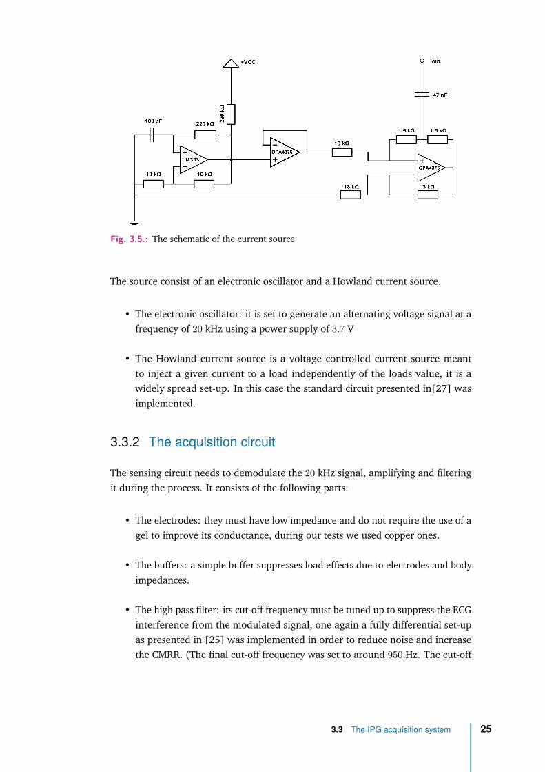
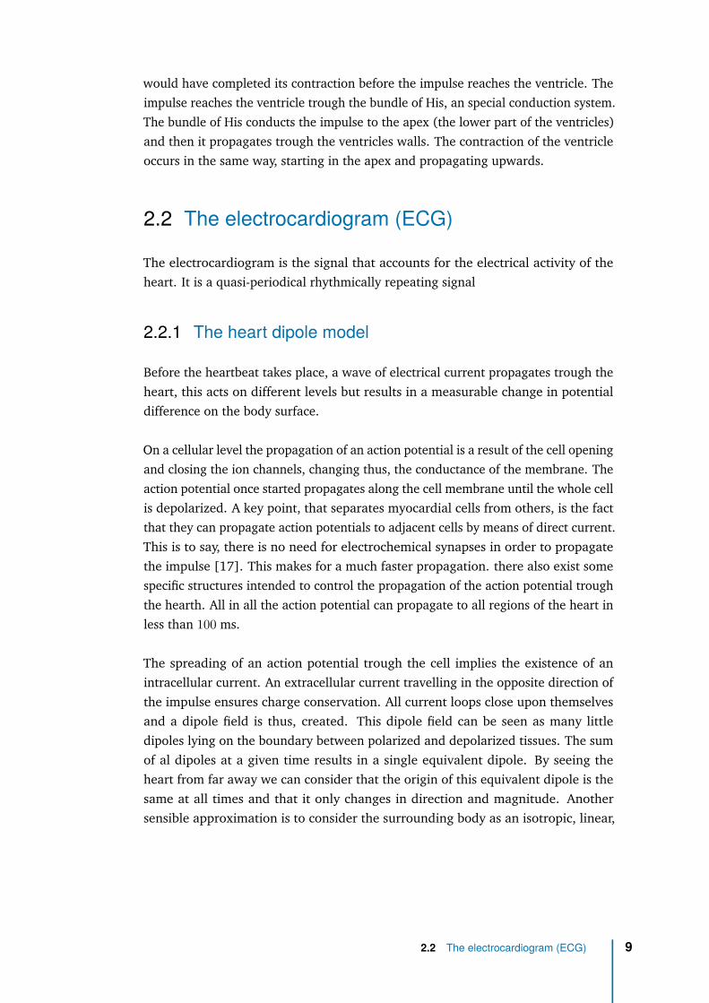
Fig. 3.5.: The schematic of the current source

The source consist of an electronic oscillator and a Howland current source.

• The electronic oscillator: it is set to generate an alternating voltage signal at afrequency of 20 kHz using a power supply of 3.7 V

• The Howland current source is a voltage controlled current source meantto inject a given current to a load independently of the loads value, it is awidely spread set-up. In this case the standard circuit presented in[27] wasimplemented.

3.3.2 The acquisition circuit

The sensing circuit needs to demodulate the 20 kHz signal, amplifying and filteringit during the process. It consists of the following parts:

• The electrodes: they must have low impedance and do not require the use of agel to improve its conductance, during our tests we used copper ones.

• The buffers: a simple buffer suppresses load effects due to electrodes and bodyimpedances.

• The high pass filter: its cut-off frequency must be tuned up to suppress the ECGinterference from the modulated signal, one again a fully differential set-upas presented in [25] was implemented in order to reduce noise and increasethe CMRR. (The final cut-off frequency was set to around 950 Hz. The cut-off


Fig. 3.6.: The schematic of the circuit

frequency was found experimentally by choosing the value that eliminated theinfluence of the ECG without altering the desired signal.

• The instrumentation amplifier: the signal needs to be amplified as much aspossible in the first stages without saturating the output. The same IA as in theECG circuit was used due to its low input noise. The gain was set to a valueof around 10. With this gain the maximum frequency before the IA starts tomisbehave is about 100 kHz. Therefore the carrier frequency can be chosenfrom the range 1− 100 kHz

• The demodulator: The circuit needs to demodulate the 20 kHz signal, thisis to say it needs to suppress the carrier frequency while maintaining theinformation enclosed on the amplitude modulation. The implemented set-upuses a switch and a comparator, chosen for their fast response, and two OpAmpchosen for its low noise. It allows for a complete recovery of the modulationthanks to the combined action of the switch and the comparator allowing thesuppression of the carrier frequency with the loss of information.

• The low-pass filter: A third order Butterworth low-pass filter was chosen for thesame reasons as in 3.2, the implemented scheme and values were taken from


[28] its cut-off frequency was set to 20 Hz as the IPG signal has a narrowerbandwidth. In addition, it provides a gain of 10.

• The amplification stage: a final amplification stage was implemented to in-crease the small signal, the pole of the amplifier circuit was set to match thecut-off frequency from the low-pass filter so both parts would work together toarchive a higher order filter. It provides a gain of about 180 which allows for agood resolution of the signal

The overall circuit has a total amplification factor of about 18000.

Fig. 3.7.: Acquired signal with the implemented set-up

Characterization

Once implemented the hardware was put to test and its characterization was made.

0.1 1 10

Frequency (Hz)

10

100

|H(s

)|

-3 /2

-

- /2

0

/2

-3 /2

-

- /2D

ela

y (

rad

ian

s)

Gain and delay

Fig. 3.8.: Transfer function of a part of the IPG circuit

The IPG circuit was also characterized, the transfer function of the second part ofthe circuit (involving the amplifier and low-pass filter but not the demodulator part)is presented in figure 3.8 were the gain and the phase delay are plotted. The studyinvolving the first part of the circuit was limited to the CMRR which yielded a valueof 51.53 dB and also the noise with both inputs connected to the ground node whichyielded a value of 4.0 mV. The noise measured for the whole circuit was of 42 mV.


4Software development

The processing of the data is of utmost importance to later on develop accurateconclusions, a careful treatment of the obtained signals was done. In this section theprincipal tools developed to retrieve information from the data are presented andexplained thoroughly.

4.1 The Pan Tompkins algorithm

The Pan Tompkins algorithm for real-time QRS detection was first presented in 1985[29] and has been, thenceforward, one of the most used algorithms for obtainingthe HR. The first step was to develop and test a custom implementation of saidalgorithm that would fulfil our needs, as a result several codes raised.

The first implementation was made in MATLAB ans can be found in A.2.1. Existingrecordings of the EGC were used to check its performance. The implemented stepsare the following:

• Filtering of the signal: a third order Butterworth bandpass filter is appliedto suppress noise and baseline wander. The bandwidth ranges from 0.5− 12Hz as it is the most cautious choice but it has been changed to a narrowerbandwidth of 5− 12 Hz for noisier data. The bandwidth can be set dependingon the acquired signal.

• Derivative operator: In order to increase the high frequency components ofthe QRS complex and diminish the low frequency components of the P and Twaves the following operator is applied:

y(n) = 18 [2x(n) + x(n− 1)− x(n− 3)− 2x(n− 4)] (4.1)

• Squaring: The squaring operator ensures the positiveness of the signal andenhances the distinguishability of the QRS complex.

28

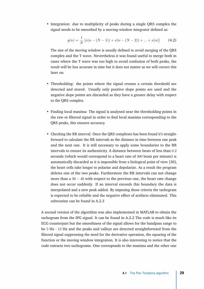
• Integration: due to multiplicity of peaks during a single QRS complex thesignal needs to be smoothed by a moving-window integrator defined as:

y(n) = 1N

[x(n− (N − 1)) + x(n− (N − 2)) + ...+ x(n)] (4.2)

The size of the moving window is usually defined to avoid merging of the QRScomplex and the T wave. Nevertheless it was found useful to merge both incases where the T wave was too high to avoid confusion of both peaks, theresult will be less accurate in time but it does not matter as we will correct thislater on.

• Thresholding: the points where the signal crosses a certain threshold aredetected and stored. Usually only positive slope points are used and thenegative slope points are discarded as they have a greater delay with respectto the QRS complex.

• Finding local maxima: The signal is analysed near the thresholding points inthe raw or filtered signal in order to find local maxima corresponding to theQRS peaks, this ensures accuracy.

• Checking the RR interval: Once the QRS complexes has been found it’s straight-forward to calculate the RR intervals as the distance in time between one peakand the next one. It is still necessary to apply some boundaries to the RRintervals to ensure its authenticity. A distance between beats of less than 0.2seconds (which would correspond to a heart rate of 300 beats per minute) isautomatically discarded as it is impossible from a biological point of view [30],the heart cells take longer to polarise and depolarize. As a result the programdeletes one of the two peaks. Furthermore the RR intervals can not changemore than a 30− 40 with respect to the previous one, the heart rate changedoes not occur suddenly. If an interval exceeds this boundary the data isinterpolated and a new peak added. By imposing those criteria the tachogramis expected to be reliable and the negative effect of artifacts eliminated. Thissubroutine can be found in A.2.3

A second version of the algorithm was also implemented in MATLAB to obtain thetachogram from the IPG signal. It can be found in A.2.2 The code is much like itsECG counterpart but the smoothness of the signal allows for the bandpass range tobe 5 Hz - 12 Hz and the peaks and valleys are detected straightforward from thefiltered signal suppressing the need for the derivative operation, the squaring of thefunction or the moving window integration. It is also interesting to notice that thecode extracts two tachograms. One corresponds to the maxima and the other one

4.1 The Pan Tompkins algorithm 29

184 186 188 190 192 194 196-0.5

0

0.5

1Input signal

184 186 188 190 192 194 196-1

-0.5

0

0.5

1

Am

plit

ude (

n.u

.)

Bandpass filter output

184 186 188 190 192 194 196

Time (seconds)

-1

-0.5

0

0.5

1Derivative operator output

184 186 188 190 192 194 196

0

0.2

0.4

0.6

0.8

Squaring operator output

184 186 188 190 192 194 196

-0.2

0

0.2

0.4

0.6

0.8

Am

plit

ude (

n.u

.)

Integrator operator output

184 186 188 190 192 194 196

Time (seconds)

-0.5

0

0.5

1Peak detected

Fig. 4.1.: The different stages of the Implemented Pan Tompkins algorithm

corresponds to the minima, this allows to compare the signal at different points withthe information from the ECG.

To prove the feasibility of a stress-sensing device based on the HRV computationit seemed necessary to implement a real time HRV detection software. The mostlogical and straightforward solution would have been the acquisition of the datadirectly in MATLAB using bluetooth technology and then, apply some minor changesto the already implemented code presented in this section. The bluetooth toolboxrequired for this solution was not available in the Linux version of MATLAB and,thus, a different approach was taken.

The next easiest solution would have been to retrieve the data directly with thecomputer communication and then use a virtual port to import it to MATLAB. Theconfiguration of the virtual ports also failed in this purpose and the data could notbe imported that way.

Finally the bluetooth communication worked using Python, with Python we couldretrieve the information and save it to a file. The file could be opened with MATLABto process the data but the continuous writing and reading of the data sooner orlater crashed the program as at some point MATLAB tries to access the file whilePython is rewriting it.

The direct communication of data between MATLAB and Python should be possibleusing a shared engine, however reached this point it did not seem like the fastestsolution. Instead the decision was taken to implement the Pan Tompkins algorithmall over in Python with the real time analysis in mind.


Fig. 4.2.: Real time implementation of the Pan Tompkins algorithm

The software acquires both ECG and IPG signals, the required filtering of bothsignals takes place and then the peaks are detected and a subroutine applies all theconditions to ensure the detected maxima corresponds to the heart-beat detection.The filtered signals alongside with their detected maxima are plotted every 3 secondswith minor delay. In figure 4.2 the output plot can be seen fro both signals. Thecode can be found in A.1.1

40 45 50 55 60 65 70

0.9

0.95

1

1.05

1.1

RR

in

terv

al (s

eco

nd

s)

Tachogram

IPG min

IPG max

ECG

0.9 0.95 1 1.05 1.1 1.15

RR interval (seconds)

0.9

0.95

1

1.05

1.1

1.15

RR

in

terv

al (s

eco

nd

s)

Tachogram ECG vs. IPG max

R2=0.986815

0.9 0.95 1 1.05 1.1 1.15

RR interval (seconds)

0.9

0.95

1

1.05

1.1

1.15Tachogram ECG vs. IPG min

R2=0.985171

Fig. 4.3.: From top to bottom, left to right: Tachogram from the three studied points, scatterplot of ECG tachogram vs. IPG maxima and minima tachogram

Once the tachograms from both signals were implemented, a check was performedto ensure a further study would make sense. Figure 4.3 shows how similar bothtachograms are and provides a good perspective for future results


4.2 Signal filtering

In order to improve the quality of the acquired signal and be able to work withacquisitions obtained from different places a filter capable of removing noise con-tamination was implemented.

The objectives set for the filter where mainly two. On the one hand the EMGinterference that arises from muscle electrical activity needed to be suppressed.EMG noise is specially present in measure from distal sites, in measurements fromfoot to foot where the subject is standing up EMG can even mask the ECG signal.Suppressing this contamination could potentially increase the range of applicationof ECG ambulatory measures.

EMG noise can not be entirely removed from the signal by means of a bandpass filterbecause its spectral bandwidth overlaps with the one of the ECG signal, by directlyfiltering EMG noise, information from ECG would also be removed. Notice that sinceIPG has a narrower bandwidth in the frequency range it is not so greatly affected byEMG and there’s no need for an additional filtering.

On the other hand, motion artifacts that arises due movements of the subject duringacquisition also troubles the processing and usually needs to be removed by hand,a filter capable or removing such artifacts would ease the post-processing of thesignals.

Before implementing the definitive filter several options where considered. A waveletbased technique as presented in [31] would fulfil our requirements, another feasiblealternative would be using some adaptive filtering algorithm such as the LMS aspresented in [32]. The main difference between both techniques is that the waveletone does not require a reference signal as opposed to the adaptive filtering whichdoes. Nevertheless the adaptive filter technique was chosen over the wavelet oneas it was found it yielded better results [23]. Over all the options available thefinal objective was to implement and test the IPNMLS filter as it has the fastestconvergence and showed better results [23]. Several kinds of data has been usedto filter the results, depending on the situation, the available information and thequality of the signals.

The first step towards the desired filter was to implement a working NMLS filterusing MATLAB, this simpler implementation allows to have a reference as well as anstarting point to tune the parameters.

4.2 Signal filtering 32

The next step was to implement the PNMLS algorithm which should have a betterperformance than the latter one in most of the cases and would ease the transitionto our definitive filter.

The last filter implement was the IPNMLS as it was the one with the better perfor-mance the filter parameters were set to the values in [24] and adjusted from there.Its implementation can be found in A.2.4

Once the definitive IPNMLS filter was implemented several tests were performed tosee if we could recover the desired waveform from corrupted signals, the performedtests used several signals from different body parts as well as several reference inputs.The references tested where:

• Other derivations of the ECG: those derivations had better quality than thenoisy signal and should be highly correlated with the desired output [23].

• An impulse train matching the heartbeat [32]: the position of the heartbeatwas obtained from either the ECG or from the IPG (maxima or minima) andwas relocated on order to match the estimated position of several points (e.g.the beginning of the P wave, the beginning of the Q wave or the peak in the Rwave) to see which position was the most suitable for our purposes.

4.3 Breath rate demodulation

Breath rate can be extracted from the signals by different means. BR acts modulatingdifferent aspects of both signals, it modifies the amplitude, base line and the HRrate [4, 5], as a result breath rate information is enclosed in those three parameters,although some present a way to mix that information [8] the objective here is toobtain a breath rate independent to the effect on the HR, the proposed analysiswill only study the retrieving of BR from amplitude and baseline modulation. Theextraction of BR from IPG signals has not been documented yet, the methods appliedrefer to those proposed for PPG signals [9] due to the similarity between both.

To extract the breath information several acquisitions of the ECG and IPG were madecontrolling the inspiration and expiration rate. The breath was kept at a constantpace and measurements for different frequencies were analysed. The frequencymodulation of the signals due to breath was discarded, and the other methods (i.e.baseline wander and amplitude modulation) were used, the reason behind is thatthe breath information is retrieved hoping that later on it can be compared with

4.3 Breath rate demodulation 33

the stress data to see the weight of respiration in the HF and LF computations. AMATLAB code was created that extracted breath information from the signals.

The baseline information was retrieved by means of a low-pass filter with 5 Hz cut-offfrequency. The amplitude modulation was calculated using the tachogram points.The envelope was calculated by interpolating the maxima and minima data, thenthe lower envelope was subtracted to the upper envelope to obtain the amplitudeinformation.

4.4 Stress measures

Stress measures were carried out by performing various test on different subjects anthen processing the recorded data.

4.4.1 The tests

Different approaches were taken in order to trigger an stress response on the subjects.Three tests were designed and implemented.

The Stroop test

Stroop test is a widespread trial that has proven to change symptovagal balance[SibolboroMezzacappa] indicating as a result a change in stress levels. Stroopeffect was first presented in [33]. The test consists on a series of colour namesshown sequentially in the screen which are written in a different colour than thename appearing. the subject is then asked to say the name of the colour in whichthe word is written (i.e. the colour of the font not the written word).

The arithmetic test

Performing simple arithmetic operations has also been proved to trigger the activa-tion of the sympathetic nervous system [14]. This tests flashed different numbersranging from −15 to 15 on-screen with varying time intervals and the subject wasasked to perform addition or subtraction consecutively.

The passive viewing of exercise

Passive viewing of exercise has shown to trigger reactions in the body similar tothose occurring when performing exercise [10]. In addition some studies show an

4.4 Stress measures 34

increase in muscular strength just by thinking about performing exercise[34, 35].Another study proves an increased benefit from exercise when subjects are awarethat the task they are performing counts as such[36]. A video recording of peopleperforming several exercise was shown to the subject with the aim of recreating atleast partially stress due to physical activity.

Developed software

For this task three codes where developed in Python. The first one, relative to theStoop test simply mixed the names and the font colours and delivered a file withboth sequences ordered indicating also if they matched or not and a second file withthe same information encoded so Python could read it.

The second code did a similar procedure mixing random numbers in the range[−15, 15], this allowed to control the results of the operations at all times and makecorrections if the subjects did any mistake.

Fig. 4.4.: Screen-shot of an instruction screen (left) and the Stroop test (right), in this casethe subject should say "green".

The third (shown in A.1.2) program used the file from the Stroop test to showon screen the names written with the corresponding colours and the file from thearithmetic test to show the sequence of operations. The code let the subjects choosein what language did they want to take the test being Catalan Spanish and Englishthe three suitable options. It also showed the instructions to perform the tests and aresting phase screen. The overall code allowed to control the times between tests bychanging the duration of the resting phase screen. In addition the intervals betweennumbers or colours could also be modified. This latter option turned out to be veryuseful when tuning the definitive test.

4.4.2 Processing the recordings

Once the test was implemented, the resting phases durations were set and theintervals of the Stroop and arithmetic tests were tuned. Several subjects were askedto perform the test. The data was recorded and analysed using MATLAB.


An additional MATLAB subroutine (shown in A.2.5) was implemented to process thedata. This program took the tachogram information and its sampling frequency andcalculated the CWT using a Morlet wavelet just as in [2]. The resulting data wasthen integrated over the LF and HF intervals and also the TP was calculated by thesame means, the output of the function returned the VLF and the TP informationover time as well as the LF and HF both normalized and not.

The processing of the recordings was made in MATLAB. The first step used the im-plemented Pan Tompkins algorithm described in section 4.1 to obtain the tachogramfrom simultaneously acquired ECG and IPG recordings. The tachograms were thenprocessed using the previously mentioned subroutine in order to retrieve both LFand HF components.


5Results and discussion

5.1 Tachogram

88 89 90 91 92 93

0.9

1

1.1

RR

in

terv

al (s

eco

nd

s)

Tachogram

IPG min

IPG max

ECG

88 89 90 91 92 93-1

0

1Filtered ECG signal

Am

plit

ud

e (

n.u

.)

88 89 90 91 92 93-1

0

1Filtered IPG signal

88 89 90 91 92 93

Time (seconds)

0.1

0.2

0.3

0.4

De

lay (

se

co

nd

s) Delay QRS-IPG

IPG min

IPG max

Fig. 5.1.: From top to bottom: Tachogram, ECG and R peaks, IPG maxima and minima,Delay between R peaks and IPG maxima and minima

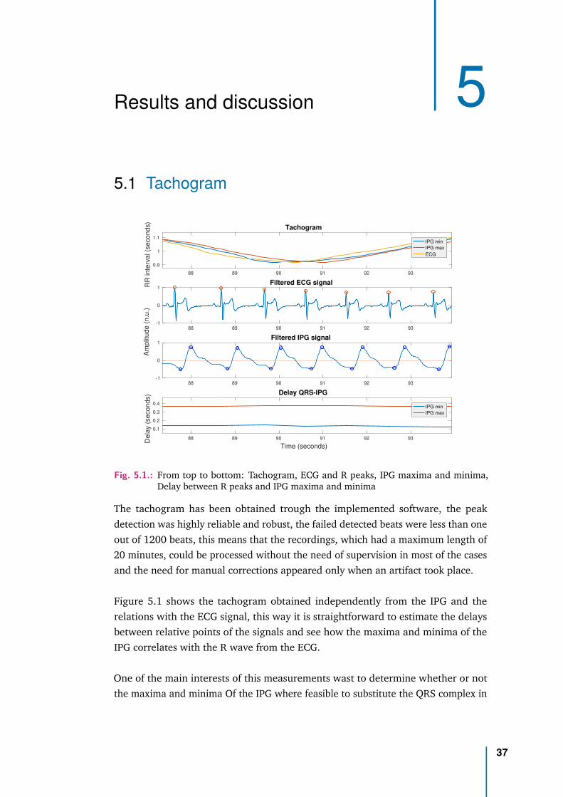
The tachogram has been obtained trough the implemented software, the peakdetection was highly reliable and robust, the failed detected beats were less than oneout of 1200 beats, this means that the recordings, which had a maximum length of20 minutes, could be processed without the need of supervision in most of the casesand the need for manual corrections appeared only when an artifact took place.

Figure 5.1 shows the tachogram obtained independently from the IPG and therelations with the ECG signal, this way it is straightforward to estimate the delaysbetween relative points of the signals and see how the maxima and minima of theIPG correlates with the R wave from the ECG.

One of the main interests of this measurements wast to determine whether or notthe maxima and minima Of the IPG where feasible to substitute the QRS complex in

37

0.85 0.9 0.95 1 1.05 1.1 1.15

Average RR interval (seconds)

-0.04

-0.03

-0.02

-0.01

0

0.01

0.02

0.03

0.04

Diffe

rence in R

R inte

rval

(EC

G -

IP

G m

ax)

(seconds)

Bland-Altman Maxima

0.9 0.95 1 1.05 1.1

Average RR interval (seconds)

-0.04

-0.03

-0.02

-0.01

0

0.01

0.02

0.03

0.04

Diffe

rence in R

R inte

rval

(EC

G -

IP

G m

in)

(seconds)

Bland-Altman Minima

Fig. 5.2.: Bland-Altman plots of the Tachogram calculated from IPG maxima (left) andminima (right) versus the one calculated from the ECG, the red lines mark the±1.96 · SD threshold

HR calculations, as shown in figure 5.1 the delay of the maxima with respect to theQRS complex remains within a narrower bounds (i.e. it has less variability) than theone calculated from the minima, this is key when using IPG signal as a substitute oras a complement of the ECG and its implications will be discussed thoroughly in thenext chapter.

Figure 4.3 showed a preliminar result, the good correlation between both tachogramsproved the similarity between the three results. A further analysis comparing bothtachograms lead to the Bland-Altman representation which is shown in figure 5.2Since the vast majority of points are within the ±1.96SD is reasonable to assumethat both signals provide almost the same information. The results are similar tothose shown in [37].

5.2 Breath rate

Breath rate was obtained from both signals using two different methods as explainedin 4.3, ECG signal allowed us to recover the breathing pace of only some recordingsand did not seem a reliable source for this information.

5.2 Breath rate 38

-0.5

0

0.5

Filtered IPG signal : Baseline modulation

6 8 10 12 14 16 18 20-1

-0.5

0

0.5

1

Time (seconds)

Am

plit

ud

e (

n.u

.)

0 0.1 0.2 0.3 0.4 0.5 0.6 0.7 0.8 0.9 1

Frequency (Hz)

0

1

2

PS

D (

s2)

Frequency estimate = 0.3 Hz

Fig. 5.3.: From top to bottom: IPG, Baseline modulation, power spectral density

IPG measurements on the other hand, showed an excellent performance recoveringthe exact pace with the baseline method as it can be seen in figure 5.3. The recordingshown here was made with pace controlled breathing of 300 mHz, the PSD of thebaseline extracted signal shows a narrow peak at that exact frequency while theone from the amplitude did not. The amplitude method yields worst results andseems unable to recover the proper rate. Other recordings made with an slowerpace, or variable breathing rate also worked when trying to recover the breathinformation with this method. As we only need to extract the information once inorder to compare it to the frequency analysis of the tachogram this results fulfilledour objective and all other methods were discarded.

Literature shows that breath pacing affects the three parameters: baseline, amplitudeand HR. The weight in each one depends on the subject and may vary, both wayswere implemented for future analysis of samples from multiple subjects.

5.3 Stress measurements

Stress tests were performed to different subjects and then analysed using the softwarepresented in section 4.4, all recordings showed a similar behaviour. In what followsexample will be presented and explained thoroughly.

The test shown in figure 5.4 featured four resting intervals of 2 minutes durationeach (0− 2 , 6− 8 , 12− 14 , 18− 20) , the arithmetical test was the first (2− 6),followed by the Stoop test (8− 12) and finishing with the exercise passive watchingtest (14− 18). The graph clearly distinguishes the beginning of the resting intervals,

5.3 Stress measurements 39

0 2 4 6 8 10 12 14 16 18 200

10

20

Pow

er

(s2)

Low Frequency component

0 2 4 6 8 10 12 14 16 18 20

0

5

10P

ow

er

(s2)

10 -5 High Frequency component

0 2 4 6 8 10 12 14 16 18 200

0.5

1

Pow

er

ratio

10 -4 Low/High Frequency ratio

Fig. 5.4.: Analysis of the recording from a test.

an increase in both LF and HF as well as the ratio between the two can be seen. Theresults seem in contradiction with each other as one may think that an increase inHF (meaning an activation of the vagal system) would relate with a decrease in LF(meaning a decreased activity of the sympathetic system).

To understand this problem with the analysis of the data the LF and HF componentswere plotted in normalized units, in figure (5.5) a different test recording is analysed.The test featured three resting intervals (0 − 3 , 7 − 10 , 14 − 16) minutes, theStoop test (3 − 7) and the passive exercise watching test (10 − 14). This time thecomponents where normalized by the TP. Thanks to this new visualization not onlythe inconsistency disappears but the resting phases are much easier to distinguishfrom the stress periods.

The same analysis can be done with the tachogram derived from IPG. IPG maxima isbetter correlated with R waves and thus should be a more suitable option to obtainsimilar results as it has been previously seen in 5.1. The tachogram obtained fromthe maxima resembles better the one from the ECG, and the delay with respect tothe R wave shows an smaller variation.

5.4 Further study of IPG signals

Once the harvesting of information from stress measures had started a differentapproach was taken. Taking advantage of the fact that a previous study on thevariability of the distance between the R wave on ECG signals and the maxima andminima of the IPG signal had already been carried out both results were combined

5.4 Further study of IPG signals 40

0 2 4 6 8 10 12 14 160

0.5

1

1.5

2Low Frequency component

Pow

er

(n.u

.)

0 2 4 6 8 10 12 14 160

0.5

1High Frequency component

0 2 4 6 8 10 12 14 160

0.5

1

Pow

er

ratio

Low/High Frequency ratio

Fig. 5.5.: Analysis of the recording from a test. This time normalized units where used

hoping for a stress indication on the variability of the distances. After having noticeda major variance on certain regions the SD of the distance relative to the maximaof the IPG was calculated over short periods of time of about 8 seconds. Thelength of the intervals were chosen trying to operate a long enough sample withoutcompromising time resolution. The retrieved results are shown in figure 5.6.

0 5 10 150

0.5

1

Pow

er

(ms

2) 10 -4 ECG High Frequency component

0 5 10 150

0.5

1

Pow

er

(ms

2) 10 -4 IPG D High Frequency component

0 5 10 150

0.5

1

1.5

Pow

er

(ms

2) 10 -4 IPG U High Frequency component

0 5 10 15

Time (minutes)

1

2

3

ST

D

Standar deviation of IPG over a 15 seconds window

Fig. 5.6.: From top to bottom: The high frequency component derived from the analysis ofthe ECG, the IPG minima and the IPG maxima and the variability of the maximapoints from IPG

This recording corresponds to a stress test with resting periods during 0− 3 , 7− 10and 14 − 16 minutes intervals, a Stroop’s test from minute 3 to 7 and a passivewatching of exercise during the 10 to 14 minutes interval. One can see that theresting intervals are clearly distinguished in both, the HF analysis and the SD plot.

5.4 Further study of IPG signals 41

The main thing one can notice when looking at the results is the resemblancebetween high frequency component and variability of the distance with the IPGmaxima. In particular it is important to notice that the SD information resemblesthe HF information derived from the tachogram obtained from the maxima. This isspecially true for noisy signals in which both HF components are not so similar.

5.5 Filtering of the ECG

117.5 118 118.5 119 119.5 120 120.50.7

0.8

0.9

1Original signal and impulse

117.5 118 118.5 119 119.5 120 120.50

0.5

1Contamined signal SNR=-40dB

Am

plit

ude (

n.u

.)

117.5 118 118.5 119 119.5 120 120.50

0.2

0.4

0.6Filter input

117.5 118 118.5 119 119.5 120 120.5

Time (seconds)

0.2

0.4

0.6

0.8

Filter output

Fig. 5.7.: From top to bottom: The original ECG, The ECG with added white noise(SNR=−40 dB), The input of the filter, The output of the filter

The filter was implemented and the parameters tuned for each set of trials, the mainobjective was to recover a signal in which one could identify the main parts (e.g.QRS complex and P and T waves), bearing this in mind parameters were tunedaccordingly.

200 200.5 201 201.5 202 202.5 203 203.5-0.2

-0.1

0

0.1

0.2

Am

plit

ud

e (

arb

. u

nits)

Input signal

200 200.5 201 201.5 202 202.5 203 203.5

Time (seconds)

-0.2

0

0.2

0.4

0.6

0.8

Am

plit

ud

e (

arb

. u

nits)

Filtered signal and reference impulse

Fig. 5.8.: Effect of our filter to an ECG recording obtained from foot to foot with the subjectstanding up. The reference was an impulse train retrieved from IPG measurements

The first test was to corrupt a good quality signal with white noise and then filter itusing an impulse train as a reference. The noise was added until no features could

5.5 Filtering of the ECG 42

be distinguished as shown in figure 5.7, then the noisy signal undergoes a simplebandpass filter before entering the adaptive filtering stage, this bandpass filter is notenough to recover the main features or to be able to distinguish between one hearthbeat and another. The signal comes out of the adaptive filtering stage with definedfeatures and could be used to calculate HR or other parameters.

299 299.5 300 300.5 301 301.5 302-0.2

-0.1

0

0.1

Am

plit

ude (

n.u

.)Input signal

299 299.5 300 300.5 301 301.5 302

Time (seconds)

-0.2

0

0.2

0.4

0.6

0.8

Am

plit

ude (

n.u

.)

Filtered signal

Fig. 5.9.: Effect of our filter to an ECG recording with a reference impulse train obtainedfrom another lead

349.5 350 350.5 351 351.5 352 352.5 353 353.5-0.2

-0.1

0

0.1

0.2Input signal

349.5 350 350.5 351 351.5 352 352.5 353 353.5

0.5

0.6

0.7

Filtered signal

349.5 350 350.5 351 351.5 352 352.5 353 353.5

time (seconds)

-1

0

1

2

3Reference signal

Fig. 5.10.: From top to bottom: Original signal, Filtered signal, Reference lead

Further tests where performed with the adaptive filtering using real noisy signalsretrieved from foot measures 5.8, or different electrodes set-ups alongside a goodquality ECG 5.9 or IPG signal. An additional complication arisen due to the unknowndelay between signals which complicated the placement of the impulses in thereference signal. Nevertheless this recordings allowed to compare the results usinganother lead (figure 5.10) or an impulse train as reference signals (figure 5.9).


We can see the great potential arising from those results, the ECG from foot to footcan be recovered with enough quality from a recording that showed little to nowindication of P, T or even R waves.

The results presented when using another lead as a reference may seem as a copy ofthe good quality lead, however in the filtered signal the U wave arises which wasnot visible in the reference one, this indicates that the retrieved signal incorporatesinformation from the original signal rather than mimicking its reference.


6Conclusions

6.1 The IPG and the HR

The retrieved tachograms from the IPG maxima and minima showed both goodcorrelation with the one obtained from QRS complex in ECG signals, this indicatesthat the same information derived from the study of HR and HRV in ECG signals canbe extracted from IPG.

It is interesting to notice how, for good quality signals, the maxima shows slightlybetter correlation with the desired tachogram. This had impact in several aspectsof this work as it indicates that the information from the maxima is more suitablefor retrieving stress information or to obtain a reference signal for the filtering ofthe ECG. This difference between maxima and minima may be due to the shapeof the signal, maxima peaks are sharper and, in general, less affected by noiseon movement, minima valleys on the other hand are duller and showed a greatersusceptibility to suffer deformations due to noise or baseline wander. During theplacement of the electrodes some minor movements sometimes caused changes inthe shape of the signal, while maxima retained its shape minima did shape-shiftreducing thus the reliability of the detected points.

In controlled measurements where the noise and movements were kept to a min-imum both points allowed to retrieve the same information about stress, and theanalysis of the three studied points yielded the same results. For good quality sig-nals the HR information can be extracted reliably, this has huge implications as itprovides a new tool for extracting all the information enclosed in the heart rate.The usefulness of this lies in the fact that IPG can be extracted from anywhere inthe body and with some electrodes configuration not feasible for retrieving ECGsignals (e.g. foot measurements with the subject standing up or with a closely placedelectrodes). Hence, IPG measurements and its derived information could substituteECG ones, yielding the same reliability and providing greater versatility.

45

6.2 Breath effect

The different modulations introduced in the signals due to breath has been studied.The breath information has been better extracted from the IPG baseline modulation.The PSD of the extracted breath signal shows that the only frequency remaining isthe one matching the controlled pacing. When we extend this analysis to recordingsmade without control of the breath pacing the spectral analysis would not show onlyone peak. It will, however, still contain mainly information about respiration. Whenthe same spectral analysis applied to the tachogram is applied to the breath signalone does not recover the same stress information.

The main objective when extracting the breath signal was to determine whetheror not the information obtained when analysing the HRV had its origin in themodulation introduced by the respiration. Since the analysis of breath rate doesnot allow to recover the stress measures there must be some additional informationenclosed in the tachogram. The analysis of HRV remains a necessary procedure toextract the symptovagal balance. The modulation and the effect of the breath isonly, if anything, partial and does not affect directly the measurements. Hence thestress tests can be performed without controlling the breath rate which simplifiesthe procedure.

6.3 Stress

The results show a clear change between the rest phases of the test and the relaxationperiods. The activation of the vagal system is made clear by an increase in theHF power. Although the increased power in the LF frequency band during therelaxation intervals would seem contradictory as it seems to indicate an increase inthe activity of the sympathetic system, it does not influence the fact that both typeof periods can be clearly distinguished. This increase was found to be as a result of ageneral increase in TP, when both components are normalized they follow opposingtendencies.

A deeper look at figure 5.5 showed some subtle details. On the one hand is possibleto see a delay in the response during the first test, as the subject only seems toincrease the activity of the sympathetic branch after the fifth minute. This delayedresponse was attributed to the test as the rate of shown words per minute was low atfirst but increased as the test advanced. Subjects were therefore, more prone to missor commit an error as time advanced. On the other hand the response of the vagalbranch seems to precede that of the sympathetic branch as HF component changesits tendency right before LF does. This has been attributed to vagal shut-down, a

6.2 Breath effect 46

process described in the literature [38] that is believed to ease the transition whena sudden stressor appears. The vagal system decreases its tone right and momentsafter the sympathetic system increases theirs, this way the change in HR is fast butnot so sharp.

The analysis of IPG signals has proven to be a feasible way to obtain stress levelsand yields the same results as the ECG derived ones. This opens the opportunity tomonitor stress levels with everyday devices such as bathroom scales or with closelyplaced electrodes which would ease the implementation. Monitoring stress levels bymeans of the IPG signal is therefore feasible but a further study should explore theway to convert this qualitative results to a continuous, everyday monitoring of stresslevels.

6.4 IPG variability; an alternative to HF analysis?

IPG and EGC signals are intrinsically different. ECG accounts for the electrical activityof the heart, this is to say it detects the impulse or the "spark" of the heartbeat but itdoes not measure the physical act of the blood leaving the heart. IPG on the otherhand measures the physical volume of blood moving trough the body, it detects theheart beat as a pressure wave that advances trough the arteries. Not only this but italso represents a weighted mean of all the contributions alongside this path.

This difference between signals allows to retrieve some useful information otherwisehidden. For example the delay between signals has proven useful to detect the stateof the arteries between the heart and the measured site [2, 18]. In this particularcase this difference can be used to detect vagal rebound. The physical properties ofIPG alongside the HR sudden changes between stress and relaxation periods surelyallows to detect changes in the way blood propagates trough the body. As the HRchanges suddenly the maxima of the IPG may change relative to the ECG wave asthe body and the blood volume takes a longer time adapting to the new pace thanthe electrical activity. This could introduce some dislocations on the IPG maxima.

A sensible assumption would be to think that this results can be extrapolated to thePPG signal and hence, an estimation of the HF component can be made by alreadyexisting devices just by studying the variability of the PPG maxima related withR waves. Nevertheless this assumption can not be made and the results can notbe extrapolated to PPG signals. As presented in [18] the IPG maxima has a timeuncertainty that can be explained due to the noise induced by the measuring systemand pink noise, its variability is not greatly affected by this small noise. On theother hand PPG measurements have an additional source of uncertainty which is

6.4 IPG variability; an alternative to HF analysis? 47

Fig. 6.1.: Estimations of the contribution of the IPG and the PPG to the uncertainty of thepulse arrival time. Taken from [18]

respiration-induced, this has a greater influence than in the previous case and thus itcan disguise the variability introduced due to stress making the explained procedureimpossible to apply to PPG technologies.

6.5 Adaptive filter

Adaptive filter has proven to be an excellent way to recover the ECG features whennoise or interference from EMG can not be eliminated by means of traditional filteringtechniques. The filter output does not only show the QRS complexes matching theheart rate but also the T waves and even the less pronounced P waves. If furtherimprovement could be done the ECG shape could provide great information evenwith an uneasy placement of the electrodes, this is to say, even when the acquiredsignal were noisy and had low quality.

One of the main advantages of this filter is the freedom to choose the referencesignal, another lead of the ECG acquired from a different place of the body, a trainof impulses derived using the ECG or the IPG or even a measurement of the EMGcan be used to suppress the noise. This provides this method with great versatilityand a huge capability to be adapted to any situation.

The proposed set-up here would be to use the IPG. IPG has a much lower contamina-tion due to EMG and can be extracted reliably from the same place (even the sameelectrodes) as the corrupted ECG signal. The IPG can then be used to extract thetrain of impulses matching the heart beats. Due to the high correlation between IPGand ECG points proved earlier this signal can work perfectly as a reference for thefilter. The filter can thus retrieve a good quality signal from a bad quality acquisition

6.5 Adaptive filter 48

without any additional measurements. Nor second ECG measurements, nor EMGmeasurements have been used in the process. New set-ups could arise from thisprocedure.

Overall the filter offers a new approach to solve the same problem. While the analysisof the IPG has shown to retrieve almost the same information as the ECG it wouldalso be possible to analyse the ECG with already studied techniques if we previouslyfilter the signal by using the IPG. Both approaches should yield similar results andboth relay in IPG measurements. A wider range of techniques allows to select thebest suited for each task, in this case the selected approach would depend on theapplication and the placement of the electrodes, as this would define the quality ofthe signal.

6.6 Future Work and perspectives

The work here presented leaves much room for further and deeper analysis.

The feasible use of IPG to obtain information about stress (or any other HRV derivedinformation for the case) has been proved. A further study with a larger populationsample and other kinds of stress-inducing tests should be performed. This wouldensure the reliability and would allow to generalize the results.

The study of other parameters related with HRV could also be made. Since ECG andHR have been deeply studied in the literature the work would consist into applyingthe existing techniques to IPG signal and prove its feasibility as ECG substitute.

The study of IPG acquired from various sites and with different electrodes configura-tion could also yield interesting results. The variability of the IPG studied here couldbe modified or affected depending on the separation of the electrodes or its location,even new information could be derived from the signal.

The filter yielded great results and allowed to recover ECG signals from contaminatedrecordings. The limits of the filter should be tested to see up to which extent thesignal of interest can be corrupted. The use of IPG opens a new range of possibilitieswhen obtaining the ECG as the electrodes can be placed without a great concernabout the quality of the signal. The number of configurations that allows to detectECG is therefore increased with the use of a filter and the simultaneous acquisitionof IPG signal.

6.6 Future Work and perspectives 49

Furthermore the filter can be improved, several parameters must be tuned up inorder to increase its capabilities. It has been noticed a great dependence on theimpulse location which is directly related with the delay between ECG and IPGsignals. A deeper study involving several subjects should allow to apply this methodto recordings from any person and thus allow for a wider application of the filter.

Overall the study of IPG altogether with ECG can have multiple applications in bothclinical and ambulatory scenarios. A huge amount of information can be derivedfrom them and a wide range of application could be develop

6.6 Future Work and perspectives 50

Bibliography

[1]Neil Schneiderman, Gail Ironson, and Scott D. Siegel. “Stress and Health: Psychological,Behavioral, and Biological Determinants”. In: Annual Review of Clinical Psychology(2005) (cit. on p. 1).

[2]Steven Vandeput. “Heart rate variability : linear and nonlinear analysis with applicationsin human physiology”. PhD thesis. 2010 (cit. on pp. 2, 3, 16, 17, 36, 47).

[3]Shelley E. Taylor, Laura Cousino Klein, Brian P. Lewis, et al. “Biobehavioral responses tostress in females: Tend-and-befriend, not fight-or-flight.” In: Psychological Review 107.3(2000), pp. 411–429 (cit. on pp. 2, 3).

[4]Peter H Charlton, Mauricio Villarroel, and Francisco Salguiero. “Waveform Analysis toEstimate Respiratory Rate”. In: Secondary Analysis of Electronic Health Records. 2016,pp. 377–390 (cit. on pp. 3, 33).

[5]Peter H Charlton, Timothy Bonnici, Lionel Tarassenko, et al. “Extraction of respiratorysignals from the electrocardiogram and photoplethysmogram: technical and physiologi-cal determinants”. In: Physiological Measurement 38.5 (May 2017), pp. 669–690 (cit. onpp. 3, 33).

[6]J M Kim, J H Hong, N J Kim, E J Cha, and T S Lee. “Two Algorithms for DetectingRespiratory Rate from ECG Signal”. In: World Congress on Medical Physics and BiomedicalEngineering 2006, Vol 14, Pts 1-6 14.27 (2007), pp. 4069–4071 (cit. on p. 3).

[7]Jesús Lázaro, Alejandro Alcaine, Daniel Romero, et al. “Electrocardiogram Derived Res-piratory Rate from QRS Slopes and R-Wave Angle”. In: Annals of Biomedical Engineering42.10 (2014), pp. 2072–2083 (cit. on p. 3).

[8]C. Orphanidou, S. Fleming, S. A. Shah, and L. Tarassenko. “Data fusion for estimatingrespiratory rate from a single-lead ECG”. In: Biomedical Signal Processing and Control8.1 (2013), pp. 98–105 (cit. on pp. 3, 33).

[9]Marco A.F. Pimentel, Alistair E.W. Johnson, Peter H. Charlton, et al. “Towards a Ro-bust Estimation of Respiratory Rate from Pulse Oximeters”. In: IEEE Transactions onBiomedical Engineering (2016), pp. 1–11 (cit. on pp. 3, 33).

[10]Rachael Brown, Ursula Kemp, and Vaughan Macefield. “Increases in muscle sympatheticnerve activity, heart rate, respiration, and skin blood flow during passive viewing ofexercise”. In: Frontiers in Neuroscience 7 JUN (2013) (cit. on pp. 3, 34).

51

[11]Anne Helene Garde, Bjarne Laursen, Anker Helms Jorgensen, and Bente Rona Jensen.“Effects of mental and physical demands on heart rate variability during computerwork”. In: European Journal of Applied Physiology 87.4-5 (2002), pp. 456–461 (cit. onp. 3).

[12]Nis Hjortskov, Dag Rissén, Anne Katrine Blangsted, et al. “The effect of mental stress onheart rate variability and blood pressure during computer work”. In: European Journalof Applied Physiology 92.1-2 (2004), pp. 84–89 (cit. on p. 3).

[13]Kurt Plarre, Andrew Raij, Syed Monowar Hossain, et al. “Continuous inference ofpsychological stress from sensory measurements collected in the natural environment”.In: 10th International Conference on Information Processing in Sensor Networks (IPSN).2011, pp. 97–108 (cit. on p. 3).

[14]E S Mezzacappa, R M Kelsey, E S Katkin, and R P Sloan. “Vagal rebound and recoveryfrom psychological stress.” In: Psychosomatic medicine 63 (2001), pp. 650–657 (cit. onpp. 3, 34).

[15]J. Wahlström, M. Hagberg, P. W. Johnson, J. Svensson, and D. Rempel. “Influence oftime pressure and verbal provocation on physiological and psychological reactionsduring work with a computer mouse”. In: European Journal of Applied Physiology 87.3(2002), pp. 257–263 (cit. on p. 3).

[16]Nadine Buard, David Campo, Roger Yu, et al. Weighing scale with extended functions.2017 (cit. on p. 4).

[17]Andrew T Reisner, Gari D Clifford, and Roger G Mark. “The Physiological Basis of theElectrocardiogram”. In: Advanced methods and tools for ECG data analysis. 2006, pp. 1,25 (cit. on p. 9).

[18]Joan Gómez-Clapers. “Assessment of trends in the cardiovascular system from timeinterval measurements using physiological signals obtained at the limbs”. PhD thesis.2015, pp. xiii, 103 (cit. on pp. 11, 13, 47, 48).

[19]Jaime Oscar Casas Piedrafita. Estudio de la relación señal a ruido en medidas debioimpedancia mediante muestreo sincrono (cit. on pp. 14, 24).

[20]E Toledo, O Gurevitz, H Hod, M Eldar, and S Akselrod. “Thrombolysis in the eyes ofthe continuous wavelet transform.” In: Computers in Cardiology, 2002, IEEE.Mi (2002),pp. 657–660 (cit. on p. 16).

[21]Paulo S. R. Diniz. Adaptive Filtering. Kluwer Academic Publishers, 2008, pp. 1–636(cit. on p. 19).

[22]Kong Aik Lee, Woon Seng Gan, and Sen M. Kuo. Subband Adaptive Filtering: Theory andImplementation. John Wiley & Sons, 2010 (cit. on p. 19).

[23]Fakroul R. Hashim, John J. Soraghan, Lykourgor Petropoulakis, and Nik G N Daud.“EMG cancellation from ECG signals using modified NLMS adaptive filters”. In: IECBES2014, Conference Proceedings - 2014 IEEE Conference on Biomedical Engineering andSciences: "Miri, Where Engineering in Medicine and Biology and Humanity Meet". 2015,pp. 735–739 (cit. on pp. 19, 20, 32, 33).

[24]Jacob Benesty and Steven L Gay. “An improved PNLMS algorithm”. In: IEEE InternationalConference on Acoustics Speech and Signal Processing. Vol. 2. August. 2002, (cit. on pp. 20,33).

Bibliography 52

[25]Oscar Casas, Enrique Mario Spinelli, and Ramón Pallás-Areny. “Fully Differential AC-Coupling Networks: A Comparative Study”. In: IEEE Transactions On InstrumentationAnd Measurement 58.1 (2009), pp. 94–98 (cit. on pp. 22, 25).

[26]American National Standards Institute. Safe current limits for electromedical apparatus.1993 (cit. on p. 24).

[27]Hassan Yazdanian, Mohsen Mosayebi Samani, and Amin Mahanm. “Characteristics ofthe Howland current source for bioelectric impedance measurements systems”. In: 201320th Iranian Conference on Biomedical Engineering, ICBME 2013. 2013, pp. 189–193(cit. on p. 25).

[28]David E. Johnson and John L. Hilburn. Rapid practical designs of active filters. JohnWiley & Sons, 1975, pp. 6–72 (cit. on p. 27).

[29]Jiapu Pan and Willis J. Tompkins. “A Real-Time QRS Detection Algorithm”. In: IEEETransactions on Biomedical Engineering BME-32.3 (1985), pp. 230–236 (cit. on p. 28).

[30]Gari D Clifford. “ECG Statistics, Noise, Artifacts, and Missing Data”. In: (2006) (cit. onp. 29).

[31]P. Mithun, Prem C. Pandey, Toney Sebastian, Prashant Mishra, and Vinod K. Pandey. “Awavelet based technique for suppression of EMG noise and motion artifact in ambulatoryECG”. In: Proceedings of the Annual International Conference of the IEEE Engineering inMedicine and Biology Society, EMBS. 2011, pp. 7087–7090 (cit. on p. 32).

[32]Nitish V. Thakor and Yi Sheng Zhu. “Applications of adaptive filtering to ECG analysis:Noise cancellation and arrhythmia detection”. In: IEEE Transactions on BiomedicalEngineering 38.8 (1991), pp. 785–794 (cit. on pp. 32, 33).

[33]J. R. Stroop. “Studies of interference in serial verbal reactions.” In: Journal of Experi-mental Psychology 18.6 (1935), pp. 643–662 (cit. on p. 34).

[34]G Yue and K J Cole. “Strength increases from the motor program: comparison oftraining with maximal voluntary and imagined muscle contractions.” In: Journal ofneurophysiology 67.5 (1992), pp. 1114–23 (cit. on p. 35).

[35]Guang H. Yue, Scott L. Wilson, Kelly J. Cole, Warren G. Darling, and William T C Yuh.“Imagined muscle contraction training increases voluntary neural drive to muscle”. In:Journal of Psychophysiology 10.3 (1996), pp. 198–208 (cit. on p. 35).

[36]Alia J. Crum and Ellen J. Langer. “Mind-set matters: Exercise and the placebo effect”.In: Psychological Science 18.2 (2007), pp. 165–171 (cit. on p. 35).

[37]N. K. Kristiansen, J. Fleischer, M. S. Jensen, K. S. Andersen, and Hans Nygaard. “Designand evaluation of a handheld impedance plethysmograph for measuring heart ratevariability”. In: Medical and Biological Engineering and Computing 43.4 (2005), pp. 516–521 (cit. on p. 38).

[38]Eran Toledo, Osnat Gurevitz, Hanoch Hod, Michael Eldar, and Solange Akselrod.“Wavelet analysis of instantaneous heart rate: a study of autonomic control duringthrombolysis”. In: American Journal of Physiology - Regulatory, Integrative and Compara-tive Physiology 284.4 (2003), R1079–R1091 (cit. on p. 47).

Bibliography 53

List of Figures

2.1 An illustration depicting the main parts of the heart . . . . . . . . . . . 82.2 An illustration depicting the main parts of electrocardiogram waveform 112.3 An illustration depicting the main parts of pulse pressure waveform . . 122.4 The use of a switch allows to use the whole signal (Taken from [19]) . 142.5 The shape of the Morlet wavelet used to process the signal . . . . . . . 182.6 The general scheme of an adaptive filter . . . . . . . . . . . . . . . . . 18

3.1 The device uses steel electrodes and connects with the tablet usingthe bitalino board (left). The insides of this device, it includes theembedded acquisition circuits, the 3.7 V battery and the bitalino board. 21

3.2 The schematic of the circuit . . . . . . . . . . . . . . . . . . . . . . . . 233.3 Acquired signal with the implemented set-up . . . . . . . . . . . . . . 233.4 Transfer function of the ECG circuit . . . . . . . . . . . . . . . . . . . . 243.5 The schematic of the current source . . . . . . . . . . . . . . . . . . . . 253.6 The schematic of the circuit . . . . . . . . . . . . . . . . . . . . . . . . 263.7 Acquired signal with the implemented set-up . . . . . . . . . . . . . . 273.8 Transfer function of a part of the IPG circuit . . . . . . . . . . . . . . . 27

4.1 The different stages of the Implemented Pan Tompkins algorithm . . . 304.2 Real time implementation of the Pan Tompkins algorithm . . . . . . . . 314.3 From top to bottom, left to right: Tachogram from the three studied

points, scatter plot of ECG tachogram vs. IPG maxima and minimatachogram . . . . . . . . . . . . . . . . . . . . . . . . . . . . . . . . . . 31

4.4 Screen-shot of an instruction screen (left) and the Stroop test (right),in this case the subject should say "green". . . . . . . . . . . . . . . . . 35

5.1 From top to bottom: Tachogram, ECG and R peaks, IPG maxima andminima, Delay between R peaks and IPG maxima and minima . . . . . 37

5.2 Bland-Altman plots of the Tachogram calculated from IPG maxima (left)and minima (right) versus the one calculated from the ECG, the redlines mark the ±1.96 · SD threshold . . . . . . . . . . . . . . . . . . . 38

5.3 From top to bottom: IPG, Baseline modulation, power spectral density 395.4 Analysis of the recording from a test. . . . . . . . . . . . . . . . . . . . 405.5 Analysis of the recording from a test. This time normalized units where

used . . . . . . . . . . . . . . . . . . . . . . . . . . . . . . . . . . . . . 41

54

5.6 From top to bottom: The high frequency component derived from theanalysis of the ECG, the IPG minima and the IPG maxima and thevariability of the maxima points from IPG . . . . . . . . . . . . . . . . 41

5.7 From top to bottom: The original ECG, The ECG with added white noise(SNR=−40 dB), The input of the filter, The output of the filter . . . . . 42

5.8 Effect of our filter to an ECG recording obtained from foot to foot withthe subject standing up. The reference was an impulse train retrievedfrom IPG measurements . . . . . . . . . . . . . . . . . . . . . . . . . . 42

5.9 Effect of our filter to an ECG recording with a reference impulse trainobtained from another lead . . . . . . . . . . . . . . . . . . . . . . . . 43

5.10 From top to bottom: Original signal, Filtered signal, Reference lead . . 43

6.1 Estimations of the contribution of the IPG and the PPG to the uncertaintyof the pulse arrival time. Taken from [18] . . . . . . . . . . . . . . . . 48

List of Figures 55

Acronyms

ANS Autonomic Nervous System.

CMRR Common-mode Rejection Ratio.

CWT Continuous Wavelet Transform.

ECG Electrocardiogram.

EMG Electromyogram.

HF High Frequency.

HR Heart Rate.

HRV Heart Rate Variability.

IPG Impedance Pletysmogram.

IPNLMS Improved Proportionate Normalized Least Mean Square.

LF Low Frequency.

LMS Least Mean Square.

NLMS Normalized Least Mean Square.

PNLMS Proportionate Normalized Least Mean Square.

56

PNS Peripheral Nervous System.

PPG Photopletysmogram.

PSD Power Spectral Density.

SD Standard Deviation.

TP Total Power.

VLF Very Low Frequency.

Acronyms 57

ACodes

A.1 Python codes

A.1.1 Real time Pan Tompkins algorithm

# This example will collect data for 5 sec.from bitalino import*import numpy as npimport matplotlib.pyplot as pltfrom drawnow import drawnowimport scipy.io as siofrom scipy import signalimport peakutilsplt.show()

#Defining the subrutine that checks the R-R intervalsdef checkdist(ntime,otime,rr,truetime,signal,timev,sf):

#confi=param[0]; hb=param[1];confi=0.3; hb=5;rri= ntime-otime;avgbeat=sum(rr[-hb:])/hb;uppbound =(1+confi)*avgbeat;lowbound =(1-confi)*avgbeat;

#If the interval is between the bounds is acceptedif rri<uppbound and rri>lowbound:

rr=np.append(rr,rri);truetime=np.append(truetime,sum(rr));lasttime=ntime

else:#if the interval is greater that the upper#bound a new beat is createdif rri>uppbound:

lstindx=np.where(timev == otime)[0][0]

58

ind=(np.argmax(signal[(lstindx+int(lowbound*sf)):(lstindx+int(uppbound*sf))])+lstindx+int(lowbound*sf));

lasttime=timev[ind]rrii=timev[ind]-otime;rr=np.append(rr,rrii);truetime=np.append(truetime,sum(rr));[rr,truetime,lasttime]=checkdist(ntime,timev[ind]

,rr,truetime,signal,timev,sf)else:#if the interval is smaller that the lower bound one of the# beats is discarded and the intervals calculated again

if rr[-1]+rri<sum(rr[-(hb+1):-2])/hb:if (abs(rr[-1]+rri-sum(rr[-(hb+1):-2])/hb) <abs(rr[-1]-sum(rr[-(hb+1):-2])/hb)):

rr[-1]=rr[-1]+rri;truetime[-1]=sum(rr)lasttime=ntime

else:lasttime=otime

else:lasttime=otime

return(rr,truetime,lasttime)

#connecting to the bitalino boardmacAddress = "20:16:07:18:17:22" #adress of our boardrunning_time = 60

batteryThreshold = 30 #chech battery levelsacqChannels = [0,1] #acquisition channels selectedsamplingRate = 100 #sampling ratenSamples = 300 #number of returned samplesdigitalOutput = [1,1]

# Connect to BITalinodevice = BITalino(macAddress)

# Start Acquisitiondevice.start(samplingRate, acqChannels)

start = time.time()end = time.time()data = numpy.empty([0,2])

A.1 Python codes 59

timeend=0.0buffsize=30*samplingRate #maximum stored data in secondsFs=float(samplingRate)szplot=8*samplingRate

#lowpass ECGWn = 12.0*2/float(Fs); NN = 3.0;[ale,ble] = signal.butter(NN,Wn,'low',analog=False);

#highpass ECGWn = 5.0*2/float(Fs); NN = 3.0;[ahe,bhe] = signal.butter(NN,Wn,'high',analog=False);

#lowpass IPGWn = 4.0*2/float(Fs); NN = 3.0;[ali,bli] = signal.butter(NN,Wn,'low',analog=False);

#highpass IPGWn = 2*0.75/float(Fs); NN = 3.0;[ahi,bhi] = signal.butter(NN,Wn,'high',analog=False);

timev=[]ecg=[]ipg=[]

#opening the plot windowplt.ion()fig = plt.figure()ax = fig.add_subplot(211)bx = fig.add_subplot(212)plt.xlabel('Time (seconds)')line1, = ax.plot(timev, ecg, 'b-')line2, = ax.plot(timev, ecg, 'r.')line4, = bx.plot(timev, ipg, 'b-')line3, = bx.plot(timev, ipg, 'r.')timeinit=0.0timeend+=float(nSamples)/float(samplingRate)try:

#this loop allows the filter to stabilize before#applying the PT algorithmwhile len(timev)<buffsize:

A.1 Python codes 60

# Read samplesdata=np.concatenate((data,

device.read(nSamples)[:,-2:]),0)data=1.0*data[-buffsize:,:]ecg=signal.detrend(data[:,0]);ipg=signal.detrend(data[:,1]);timev=np.concatenate((timev,np.linspace(

timeinit,timeend,nSamples+1)[1:]),0)timev=1.0*timev[-buffsize:]timeinit=timev[-1]timeend+=float(nSamples)/float(samplingRate)

#filter the dataecg2 = signal.filtfilt(ale,ble,ecg);ecg2 = signal.filtfilt(ahe,bhe,ecg2);ipg2 = signal.filtfilt(ali,bli,ipg);ipg2 = signal.filtfilt(ahi,bhi,ipg2);

line1.set_ydata(ecg[-szplot:]/max(ecg[-szplot:]))line1.set_xdata(timev[-szplot:])

#updating the plotline4.set_ydata(ipg2[-szplot:]/max(ipg2[-szplot:]))line4.set_xdata(timev[-szplot:])ax.relim()ax.autoscale_view()bx.relim()bx.autoscale_view()

fig.canvas.draw()plt.draw()

ecg2 = signal.filtfilt(ale,ble,ecg);ecg2 = signal.filtfilt(ahe,bhe,ecg2);ipg2 = signal.filtfilt(ali,bli,ipg);ipg2 = signal.filtfilt(ahi,bhi,ipg2);

Indexes = peakutils.indexes(ipg2/max(ipg2[-10*samplingRate:]),thres=np.mean(ipg2[-10*samplingRate:]),min_dist=0.5*samplingRate)rr=np.array(timev[Indexes[-6:-1]]-timev[Indexes[-7:-2]])rr2=np.array(timev[Indexes[-6:-1]]-timev[Indexes[-7:-2]])truetime=rr.dot(np.triu(np.ones((5,5))))truetime2=rr.dot(np.triu(np.ones((5,5))))

A.1 Python codes 61

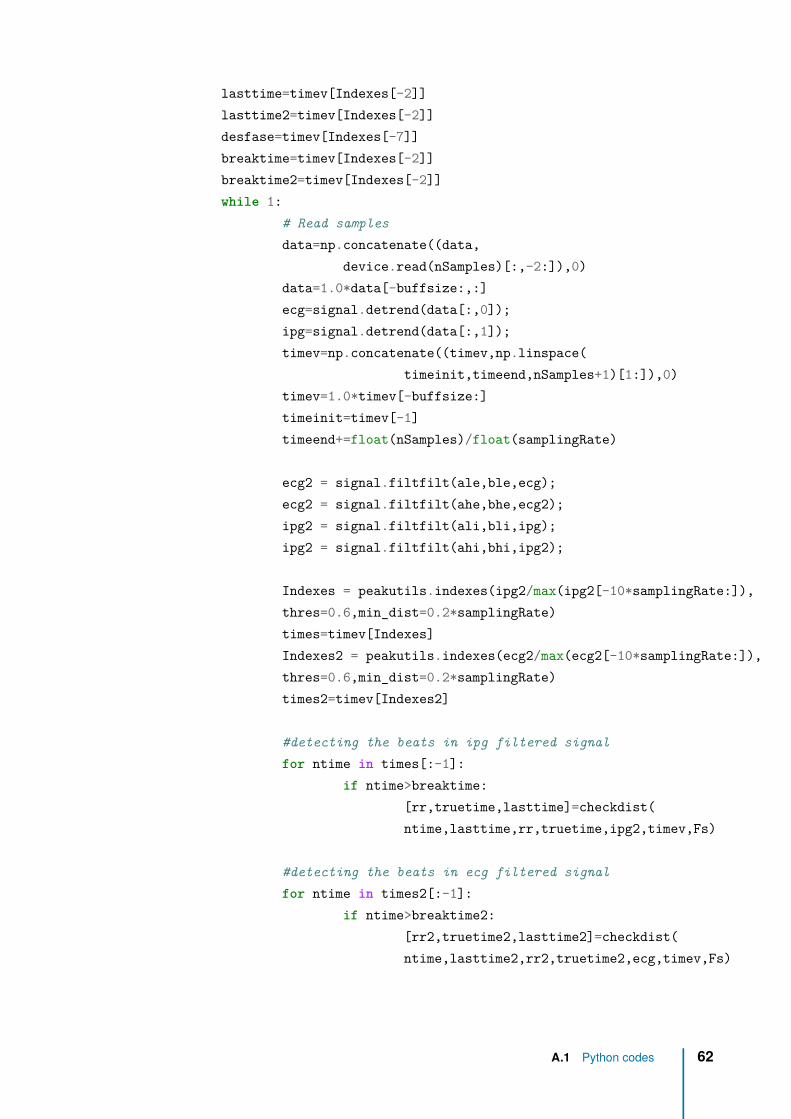
lasttime=timev[Indexes[-2]]lasttime2=timev[Indexes[-2]]desfase=timev[Indexes[-7]]breaktime=timev[Indexes[-2]]breaktime2=timev[Indexes[-2]]while 1:

# Read samplesdata=np.concatenate((data,

device.read(nSamples)[:,-2:]),0)data=1.0*data[-buffsize:,:]ecg=signal.detrend(data[:,0]);ipg=signal.detrend(data[:,1]);timev=np.concatenate((timev,np.linspace(

timeinit,timeend,nSamples+1)[1:]),0)timev=1.0*timev[-buffsize:]timeinit=timev[-1]timeend+=float(nSamples)/float(samplingRate)

ecg2 = signal.filtfilt(ale,ble,ecg);ecg2 = signal.filtfilt(ahe,bhe,ecg2);ipg2 = signal.filtfilt(ali,bli,ipg);ipg2 = signal.filtfilt(ahi,bhi,ipg2);

Indexes = peakutils.indexes(ipg2/max(ipg2[-10*samplingRate:]),thres=0.6,min_dist=0.2*samplingRate)times=timev[Indexes]Indexes2 = peakutils.indexes(ecg2/max(ecg2[-10*samplingRate:]),thres=0.6,min_dist=0.2*samplingRate)times2=timev[Indexes2]

#detecting the beats in ipg filtered signalfor ntime in times[:-1]:

if ntime>breaktime:[rr,truetime,lasttime]=checkdist(ntime,lasttime,rr,truetime,ipg2,timev,Fs)

#detecting the beats in ecg filtered signalfor ntime in times2[:-1]:

if ntime>breaktime2:[rr2,truetime2,lasttime2]=checkdist(ntime,lasttime2,rr2,truetime2,ecg,timev,Fs)

A.1 Python codes 62

breaktime=times[-2];breaktime2=times2[-2];trueindex=np.rint((truetime-timev[0]+desfase)*(buffsize+1)/(timev[-1]-timev[0]))trueindex=trueindex.astype(int)-2trueindex2=np.rint((truetime2-timev[0]+desfase)*(buffsize+1)/(timev[-1]-timev[0]))trueindex2=trueindex2.astype(int)-2print trueindex[-5:],Indexes[-6:-1]#print Indexes,truetime#refresh the plotsline1.set_ydata(ecg[-szplot:]/max(ecg[-szplot:]))line1.set_xdata(timev[-szplot:])line2.set_ydata(ecg[trueindex2[-5:]]/max(ecg[-szplot:]))line2.set_xdata(timev[trueindex2[-5:]])#line2.set_ydata(ecg2[-szplot:]/max(ecg2[-szplot:]))#line2.set_xdata(timev[-szplot:])#line3.set_ydata(ipg[-szplot:]/max(ipg[-szplot:]))#line3.set_xdata(timev[-szplot:])line3.set_ydata(ipg2[trueindex[-5:]]/max(ipg2[-szplot:]))line3.set_xdata(timev[trueindex[-5:]])line4.set_ydata(ipg2[-szplot:]/max(ipg2[-szplot:]))line4.set_xdata(timev[-szplot:])ax.relim()ax.autoscale_view()bx.relim()bx.autoscale_view()

fig.canvas.draw()plt.draw()

except KeyboardInterrupt:print 'interrupted!'

# Turn BITalino led ondevice.trigger(digitalOutput)# Stop acquisitiondevice.stop()# Close connectiondevice.close()

A.1 Python codes 63

A.1.2 Stroop test implementation

# -*- encoding: utf-8 -*-

import pygame, sysfrom pygame.locals import *import random

#define the color codes and its the printed outputWHITE = (255,255,255)BLACK = (0,0,0)RED = (255,0,0)GREEN = (0,255,0)BLUE = (0,0,255)YELLOW = (255,255,0)ORANGE = (255,128,0)PINK = (255,0,255)

cWHITE = '(255,255,255)'cBLACK = '(0,0,0)'cRED = '(255,0,0)'cGREEN = '(0,255,0)'cBLUE = '(0,0,255)'cYELLOW = '(255,255,0)'cORANGE = '(255,128,0)'cPINK = '(255,0,255)'

#Making the list with the names and tyhe codes (must have same order)COULEURS = (WHITE,BLACK,RED,GREEN,BLUE,YELLOW,ORANGE,PINK)TEXTE_COULEURS = ("WHITE","BLACK","RED","GREEN","BLUE","YELLOW","ORANGE","PINK")COULEURS_CODE = (cWHITE,cBLACK,cRED,cGREEN,cBLUE,cYELLOW,cORANGE,cPINK)

# Colour feedback and insctructionsNOIR = (0, 0, 0)#Colour of the backgroundFOND = (200,200,200)

#this subroutine defines the color names depending on the selected languagedef name_colors():

print "Idioma/Language? (Català/castellano/English)"Lan = raw_input()

A.1 Python codes 64

if Lan == "Català" or Lan == "català" or Lan == "catala" or Lan == "Catala":Lan = "Català"TEXTE = ("BLANC","NEGRE","VERMELL","VERD","BLAU","GROC","TARONJA","ROSA")else:if Lan == "Castellano" or Lan == "castellano":Lan = "Castellano"TEXTE = ("BLANCO","NEGRO","ROJO","VERDE","AZUL","AMARILLO","NARANJA","ROSA")else:if Lan=="English" or Lan=="english":Lan = "English"TEXTE = ("WHITE","BLACK","RED","GREEN","BLUE","YELLOW","ORANGE","PINK")else:print "Wut? Try again"Lan, TEXTE=name_colors()return Lan, TEXTE

def attente():start = Falsepygame.event.get()while not start:

for e in pygame.event.get():if e.type == KEYDOWN:

if e.key == K_SPACE:start = True

elif e.key == K_ESCAPE:raise Exception

#this routine displays the color names encoded in the text filesdef stroop_et_sisi(TEXTE, fenetre, filec, delay, rep):

font = pygame.font.Font(None, 50)nombre_essai = 0for i in range(rep):

fenetre.fill(FOND)position=S/2line=filec.readline(); line=line.strip('\n\r'); line=line.split()MY_TEXT = font.render(TEXTE[COULEURS_CODE.index(line[1])]

, 1, COULEURS[COULEURS_CODE.index(line[0])])#t0 = pygame.time.get_ticks()#print t0MY_TEXT_POSITION = MY_TEXT.get_rect()MY_TEXT_POSITION.center = fenetre.get_rect().center

A.1 Python codes 65

fenetre.blit(MY_TEXT, [position-MY_TEXT.get_width()/2, position-MY_TEXT.get_height()/2])

pygame.display.flip()pygame.time.wait(delay)

return ()

#this subroutine displays the arithmetic operations encoded in the text filesdef arith(fenetre, filec, delay, rep):

font = pygame.font.Font(None, 50)nombre_essai = 0for i in range(rep):

fenetre.fill(FOND)position=S/2line=filec.readline(); line=line.strip('\n\r'); line=line.split()MY_TEXT = font.render(line[0], 5, NOIR)#t0 = pygame.time.get_ticks()#print t0MY_TEXT_POSITION = MY_TEXT.get_rect()MY_TEXT_POSITION.center = fenetre.get_rect().centerfenetre.blit(MY_TEXT, [position-MY_TEXT.get_width()/2

, position-MY_TEXT.get_height()/2])pygame.display.flip()pygame.time.wait(delay)

return ()

#this subroutine displays the resting period textdef pause(fenetre, Lan):

pygame.font.initfenetre.fill(FOND)font = pygame.font.Font(None, 30)

if Lan=="Català":

text = (u"Respira profundament.",u"Durant els pròxims 2 minuts relaxa't",u"No et moguis ni deixis anar els elèctrodes!",u"",u"En breu rebràs instruccions sobre la següent tasca")

text2 = (u"Inspira",u"Aguanta",

A.1 Python codes 66

u"Expira")

if Lan=="Castellano":

text = (u"Respira profundamente",u"Durante los próximos 2 minutos relájate",u"No te muevas ni sueltes los electrodos",u"",u"En breve recibirás instrucciones",u"acerca de la próxima tarea")

text2 = (u"Inspira",u"Aguanta",u"Expira")

if Lan=="English":text = (u"Take a deep breath",u"During the following 2 minutes relax.",u"Do not move or let go the electrodes.",u"",u"Shortly you will receieve instructions",u"about the following task")

text2 = (u"Inspire",u"Hold on",u"Expire")

for i in range(len(text)):ordonnee_ligne= 150 + 40*iMY_TEXT= font.render(text[i], 1, NOIR)fenetre.blit(MY_TEXT, [20, ordonnee_ligne])pygame.display.flip()pygame.time.wait(1000)

#breath_mod(fenetre, text2)pygame.time.wait(153000)

#This subroutine can be activated to control breath#pacing during the resting perioddef breath_mod(fenetre, text2):

pygame.font.initfont = pygame.font.Font(None, 30)

A.1 Python codes 67

ordonnee_ligne1= 150 + 40*6ordonnee_ligne2= 150 + 40*7ordonnee_ligne3= 150 + 40*8

for i in range(9):ordonnee_ligne1= 150 + 40*6MY_TEXT= font.render(text2[2], 1, FOND)fenetre.blit(MY_TEXT, [20, ordonnee_ligne3])pygame.display.flip()MY_TEXT= font.render(text2[0], 1, NOIR)fenetre.blit(MY_TEXT, [20, ordonnee_ligne1])pygame.display.flip()for j in range(4):

MY_TEXT= font.render(str(j+1), 1, NOIR)fenetre.blit(MY_TEXT, [170+40*j, ordonnee_ligne1])pygame.display.flip()pygame.time.wait(1000)MY_TEXT= font.render(str(j+1), 1, FOND)fenetre.blit(MY_TEXT, [170+40*j, ordonnee_ligne1])pygame.display.flip()

MY_TEXT= font.render(text2[0], 1, FOND)fenetre.blit(MY_TEXT, [20, ordonnee_ligne1])pygame.display.flip()

MY_TEXT= font.render(text2[1], 1, NOIR)fenetre.blit(MY_TEXT, [20, ordonnee_ligne2])pygame.display.flip()for j in range(6):


MY_TEXT= font.render(text2[1], 1, FOND)fenetre.blit(MY_TEXT, [20, ordonnee_ligne2])pygame.display.flip()

A.1 Python codes 68

MY_TEXT= font.render(text2[2], 1, NOIR)fenetre.blit(MY_TEXT, [20, ordonnee_ligne3])pygame.display.flip()for j in range(7):


#this subroutine displays the Stroop instructionsdef instructions1(fenetre, Lan):

pygame.font.initfenetre.fill(FOND)font = pygame.font.Font(None, 30)if Lan=="Català":

text = (u"Prepara't!",u"A continuació apareixeran els noms d'alguns",u"colors escrits a la pantalla.",u"Digues en veu alta el color de les lletres,",

u"no et confonguis amb la paraula que esta escrita")


text = (u"Prepárate!",u"A continuación aparecerán los nombres de algunos",u"colores escritos en la pantalla.",u"Di en voz alta el color de las letras",

u"No te confundas con la palabra que está escrita")

if Lan=="English":text = (u"Get ready!",

u"Now the name of some colours will appear",u"written on the screen.",u"Say out loud the colour of the letters",

u"do not get confused with the written word")

for i, txt in enumerate(text):

A.1 Python codes 69

ordonnee_ligne= 20 + 40*iMY_TEXT= font.render(txt, 1, NOIR)fenetre.blit(MY_TEXT, [15, ordonnee_ligne])pygame.time.wait(1000)pygame.display.flip()

pygame.time.wait(16000)

#this subroutine displays the aritmethic test instructionsdef instructions2(fenetre, Lan):


if Lan=="Català":

text = (u"Prepara't",u"Aquesta tasca consisteix en sumar i restar.",u"Suma o resta al nombre anterior els nombres",u"que apareixeran en la pantalla.",u"Digues el resultat en veu alta.",u"Si et perds algun nombre no passa res",u"simplement digues algun nombre i continua",u"a partir d'aquell",u"",u"El primer nombre es:",u"497")


text = (u"Prepárate",u"Esta tarea consiste en sumar y restar",u"Suma o resta al anterior numero los números",u"que vayan apareciendo en pantalla.",u"Di el resultado en voz alta.",u"si te pierdes algún numero no pasa nada",u"simplemente di algún numero y continua desde ese"u"",u"El primer número es:",u"497")

if Lan=="English":text = (u"Get ready",

A.1 Python codes 70

u"This task consist in adding and subtracting",u"Add or subtract to the previous number the numbers",u"that appear on the screen.",u"Say the result out loud",u"If you miss a number don't worry",u"just say some number and continue from that",u"",u"The first number is:",u"497")



#this subroutine displays the passive exercise instructionsdef instructions3(fenetre, Lan):# affiche les instructions, ligne par ligne


if Lan=="Català":

text = (u"Prepara't",u"Aquesta tasca consisteix en visualitzar un vídeo.",u"Ignora qualsevol text que aparegui i centra't",u"en els exercicis que es mostraran",u"Intenta involucrar-te tant com puguis sense moure't.",u"En particular presta atenció als grups de músculs ",u"que s'exerciten en cada moment")


text = (u"Prepárate",u"Esta tarea consiste en visualizar un video.",u"Ignora cualquier texto que aparezca y céntrate",u"en los ejercicios que se mostraran",

A.1 Python codes 71

u"Intenta involucrarte tanto como puedas sin moverte.",u"En particular presta atención a los grupos de músculos ",u"que se ejerciten en cada momento")

if Lan=="English":text = (u"Get ready",u"This task consist in watching a movie.",u"Ignore any text that may appear and focus",u"on the exercises that will be shown",u"Try to engage as much as possible without moving.",u"In particuklar pay attention to the muscles",u"involved in each exercise")



#starting the main loopdef main():#creation fichier et creation en-tetes

Lan, TEXTE = name_colors()

fenetre = pygame.display.set_mode([S, S])pygame.display.set_caption('Simon-Stroop')

# pause(fenetre, Lan) #resting period# instructions2(fenetre, Lan) #arithmetic instructions#

#performing the test with 6 seconds interval# col_file = open("6seconds_arith.txt","r")# arith(fenetre, col_file, 5999, 10)# col_file.close()## #performing the test with 5 seconds interval# col_file = open("5seconds_arith.txt","r")# arith(fenetre, col_file, 4999, 12)# col_file.close()

A.1 Python codes 72

## #performing the test with 4 seconds interval# col_file = open("4seconds_arith.txt","r")# arith(fenetre, col_file, 3999, 15)# col_file.close()## #performing the test with 3 seconds interval# col_file = open("3seconds_arith.txt","r")# arith(fenetre, col_file, 2999, 20)# col_file.close()

pause(fenetre, Lan) #resting perodinstructions1(fenetre, Lan) #Stroop instructions

# #performing the test with 2 seconds intervalcol_file = open("2seconds_code.txt","r")stroop_et_sisi (TEXTE, fenetre, col_file, 1999, 15)col_file.close()

# #performing the test with 1.5 seconds intervalcol_file = open("15seconds_code.txt","r")stroop_et_sisi (TEXTE, fenetre, col_file, 1499, 60)col_file.close()

# #performing the test with 1 seconds intervalcol_file = open("1seconds_code.txt","r")stroop_et_sisi (TEXTE, fenetre, col_file, 999, 120)col_file.close()

pause(fenetre, Lan) #resting periodinstructions3(fenetre, Lan) #exercise instructions

try:pygame.init()main()

finally:pygame.quit()

A.1 Python codes 73

A.2 Matlab codes

A.2.1 ECG Pan Tompkins algorithm

function [signal,tachogram,Indexes,Frr]=PT_ECG(InECG,Fs)x=detrend(InECG);M=length(x); intrange=round(5*Fs/20);der=zeros(1,M); Pulse=zeros(1,M);timevec=linspace(0,M/Fs,M);hb=5; %Number of heartbeats to averageldelay=.13; %aprox Delay of the negtive slope with respect to the r waveudelay=.05; %aprox Delay of the positive slope with respect to the r waveconfi=.3; %Maximum variation from one hearbeat with respect to the othersFrr=8; %Sampling frequency of the tachogram

Wn = 45/Fs;NN = 3; % order of 3 less processing[a,b] = butter(NN,Wn,'low'); %bandpass filteringy = filtfilt(a,b,x);y = y/ max(abs(y));Wn = .5/Fs;NN = 3; % order of 3 less processing[a,b] = butter(NN,Wn,'high'); %bandpass filteringfECG = filtfilt(a,b,y);fECG = fECG/ max(abs(fECG));

for i=5:Mder(i)=(2*fECG(i)+fECG(i-1)-fECG(i-3)-2*fECG(i-4))/8;%derivative operatorend

derr=detrend(der).*detrend(der);%squaring operator

for n=intrange:MPulse(n)=sum(derr(n-intrange+1:n))/intrange;%Integratorend

%setting the treshold for detecting the rising and falling slopestreshold=mean(ecg);QRSStart=[]; QRSEnd=[];

for i = 1:length(ecg)-1

A.2 Matlab codes 74

%detect if the signal crosses the slope and save its indexif Pulse(i) <= treshold && Pulse(i+1) > treshold

QRSStart = [QRSStart i];endif Pulse(i) <= treshold && Pulse(i+1) > treshold

QRSEnd = [QRSEnd i];end

end

Indexes=zeros(1,length(QRSStart));for i=1:length(QRSStart)

%search for the maximum point arround the tresholde crossing points[~,ind]=max(fECG(QRSStart(i)-round(ldelay*Fs):QRSStart(i)+round(udelay*Fs)));Indexes(i)= ind+QRSStart(i)-round(ldelay*Fs)-1;

end

%define the interval vectorrr=[Indexes(2)-Indexes(1)]; truetime=[rr(1)];i=2;Indexes=Indexes';while i<length(Indexes)

if i>=hb+1bb=hb;

elsebb=i-1;

end%define the tresholdsavgbeat=sum(rr(end-bb+1:end))/bb;uppbound =(1+confi)*avgbeat;lowbound =(1-confi)*avgbeat;%check the RR intervals[rr,Indexes,i]=tach_check(uppbound,lowbound,rr,Indexes,fECG,Fs,i);

end%interpolate the tachogram for evenly spaced dataMM=round(Frr*truetime(end)/(2*Fs))*2;truetime2=linspace(truetime(1),truetime(end),MM);tacho = interp1(truetime,rr,truetime2, 'pchip');%store the signal and the tachogramsignal=[timevec',fECG];tachogram=[truetime2'/Fs,tacho'/Fs];return

A.2 Matlab codes 75

A.2.2 IPG Pan Tompkins algorithm

function [signal,tachogramD,tachogramU,IndexesD,IndexesU,Frr]=PT_IPG2(InIPG,Fs)x=detrend(InIPG);M=length(x); intrange=round(6*Fs/20);der=zeros(1,M); egc=NaN(1,M);timevec=linspace(0,M/Fs,M);hb=5; %Number of heartbeats to averageconfi=.4; %Maximum variation from one hearbeat with respect to the othersFrr=8; %Sampling frequency of the tachogram

Wn = 4*2/Fs;NN = 3; % order of 3 less processing[a,b] = butter(NN,Wn,'low'); %bandpass filteringy = filtfilt(a,b,x);y = y/ max(abs(y));Wn = 2*0.75/Fs;NN = 3; % order of 3 less processing[a,b] = butter(NN,Wn,'high'); %bandpass filteringfIPG = filtfilt(a,b,y);fIPG = fIPG/ max(abs(fIPG));fIPG=detrend(fIPG);

%finding the minima separated apart by a distance of .4 seconds[Minima,MinIdx] = findpeaks(-1*fIPG,'MinPeakDistance',.4*Fs); Minima=-Minima;MinIdx=MinIdx(find(Minima < mean(fIPG)));%finding the maxima separated apart by a distance of .4 seconds[Maxima,MaxIdx] = findpeaks(fIPG,'MinPeakDistance',.4*Fs);MaxIdx=MaxIdx(find(Maxima > mean(fIPG)));

IndexesD=MinIdx; IndexesU=MaxIdx; %defining the indexes of the tachogramRRD=[IndexesD(2)-IndexesD(1)]; i=2;%calculating the intervals of the tachogram

while i<length(IndexesD) %checking the RR intervalsif i>hb

bb=hb;else

bb=i-1;end%calculating the confidence intervalsavgbeat=sum(RRD(end-bb+1:end))/bb;

A.2 Matlab codes 76

uppbound =(1+confi)*avgbeat;lowbound =(1-confi)*avgbeat;[RRD,IndexesD,i]=tach_check2(uppbound,lowbound,RRD,IndexesD,-fIPG,Fs,i);

end

truetimeD=IndexesD(1:end-1)/Fs;%defining the time vector

%calculating the intervals of the tachogramRRU=[IndexesU(2)-IndexesU(1)];i=2;

while i<length(IndexesU)%checking the RR intervalsif i>hb

bb=hb;else

bb=i-1;end%calculating the confidence intervalsavgbeat=sum(RRU(end-bb+1:end))/bb;uppbound =(1+confi)*avgbeat;lowbound =(1-confi)*avgbeat;[RRU,IndexesU,i]=tach_check1(uppbound,lowbound,RRU,IndexesU,fIPG,Fs,i);

end

truetimeU=IndexesU(1:end-1)/Fs;%defining the time vector

%interpolating to get evenly spaced tachogram dataMMD=round(Frr*(truetimeD(end)-truetimeD(1)));MMU=round(Frr*(truetimeU(end)-truetimeU(1)));truetime2D=linspace(truetimeD(1),truetimeD(end),MMD);truetime2U=linspace(truetimeU(1),truetimeU(end),MMU);tachoU = interp1(truetimeU',RRU,truetime2U, 'pchip');tachoD = interp1(truetimeD',RRD,truetime2D, 'pchip');

%saving the signal and tachogram informationsignal=[timevec',fIPG];tachogramD=[truetime2D',tachoD'/Fs];tachogramU=[truetime2U',tachoU'/Fs];

return

A.2 Matlab codes 77

A.2.3 RR interval check

function [rr,Indexes,j]=tach_check(uppbound,lowbound,rr,Indexes,ecg2,Fs,j)rri= Indexes(j+1)-Indexes(j); %calculate the intervalif rri<uppbound && rri>lowbound %If it is within bounds it is accepted

rr=[rr,rri];else

if rri>uppbound || rri>2*Fs %if its too long a new beat is interpolated[~,ind]=max(ecg2(Indexes(j)+round(lowbound):Indexes(j)+round(uppbound)));rr=[rr,round(lowbound)+ind-1];Indexes=[Indexes(1:j);Indexes(j)+round(lowbound)+ind-1;Indexes(j+1:end)];

endif rri<lowbound || rri<.2*Fs%If it is too short one of the beats gets discarded

if j>6%greater amplitude criteria

% if ecg2(Indexes(j))>ecg2(Indexes(j+1))%greater similarity criteria

if abs(5*rr(end)-sum(rr(end-5:end-1)))<abs(...5*(rr(end)+rri)-sum(rr(end-5:end-1)))

Indexes(j+1)=[];if j<length(Indexes)

% if the last beat is incorrect it is supressed and% recalculated[rr,Indexes,j]=tach_check(...uppbound,lowbound,rr,Indexes,ecg2,Fs,j);j=j-1;

endelse

Indexes(j)=[];rr(end)=rr(end)+rri;if j<length(Indexes)

% if the first beat is incorrect it is supressed and% recalculated[rr,Indexes,j]=tach_check(...uppbound,lowbound,rr,Indexes,ecg2,Fs,j);j=j-1;

endend

elseIndexes=Indexes(j+1:end);

A.2 Matlab codes 78

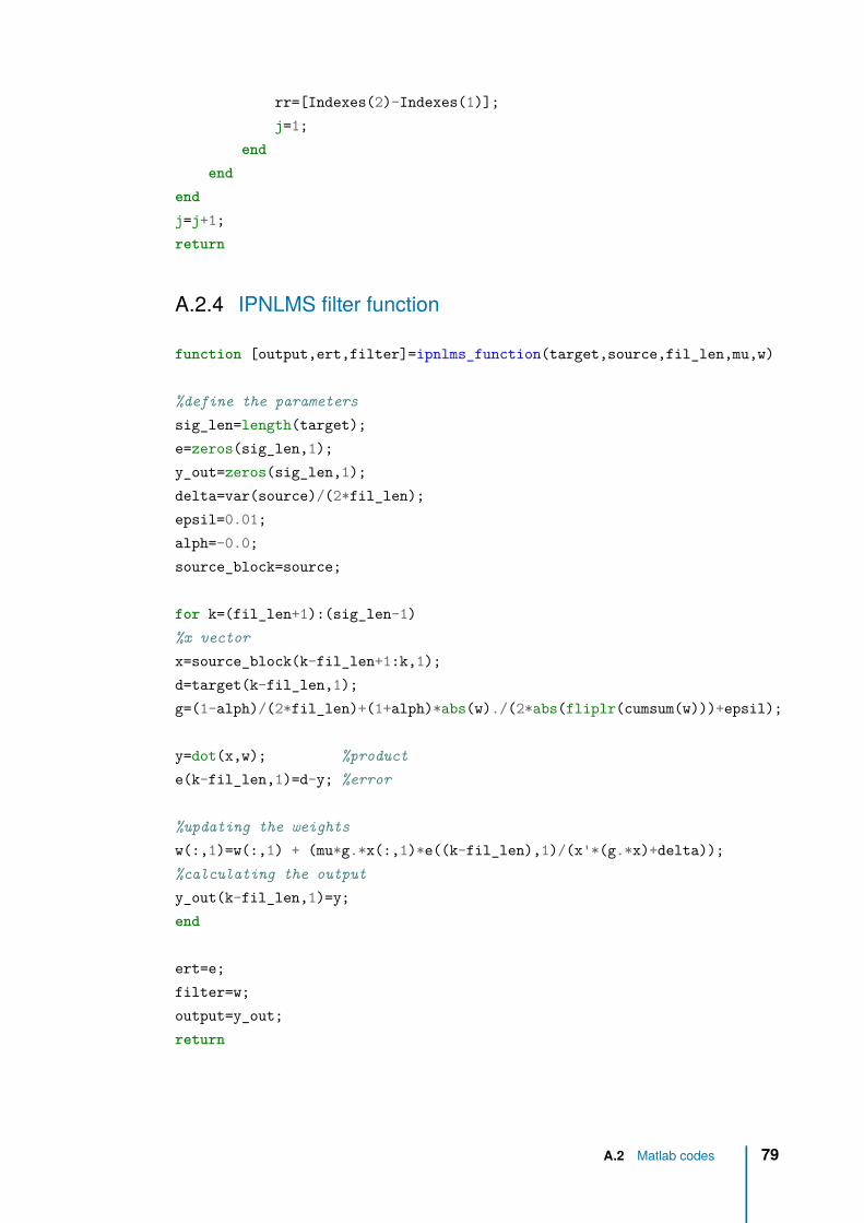
rr=[Indexes(2)-Indexes(1)];j=1;

endend

endj=j+1;return

A.2.4 IPNLMS filter function

function [output,ert,filter]=ipnlms_function(target,source,fil_len,mu,w)

%define the parameterssig_len=length(target);e=zeros(sig_len,1);y_out=zeros(sig_len,1);delta=var(source)/(2*fil_len);epsil=0.01;alph=-0.0;source_block=source;

for k=(fil_len+1):(sig_len-1)%x vectorx=source_block(k-fil_len+1:k,1);d=target(k-fil_len,1);g=(1-alph)/(2*fil_len)+(1+alph)*abs(w)./(2*abs(fliplr(cumsum(w)))+epsil);

y=dot(x,w); %producte(k-fil_len,1)=d-y; %error

%updating the weightsw(:,1)=w(:,1) + (mu*g.*x(:,1)*e((k-fil_len),1)/(x'*(g.*x)+delta));%calculating the outputy_out(k-fil_len,1)=y;end

ert=e;filter=w;output=y_out;return

A.2 Matlab codes 79

A.2.5 Frequency analysis for stress detection

function [VLF,LF,HF,TP,LFn,HFn]=freqevol(y,fs)

[wt,f] = cwt(y,'amor',fs); %calculating the CWT

II = length(y);%setting the boundarieslowerb = knnsearch(f,0);upperb = knnsearch(f,1);vlfb = knnsearch(f,0.04);lfb = knnsearch(f,0.15);hfb = knnsearch(f,0.4);VLF=NaN(1,II); LF=NaN(1,II);HF=NaN(1,II); TP=NaN(1,II);

%integrating all components at each momentfor i=1:IIVLF(i)=trapz(f(lowerb:-1:vlfb),abs(wt(lowerb:-1:vlfb,i)).^2);LF(i)=trapz(f(vlfb:-1:lfb),abs(wt(vlfb:-1:lfb,i)).^2);HF(i)=trapz(f(lfb:-1:hfb),abs(wt(lfb:-1:hfb,i)).^2);TP(i)=trapz(f(lowerb:-1:upperb),abs(wt(lowerb:-1:upperb,i)).^2);end%calculating the normalized componentsLFn=LF./(TP-VLF); HFn=HF./(TP-VLF);return

A.2 Matlab codes 80

heart rate variability acquisition from ambulatory

Documents