healthy beaches tampa bay: microbiological monitoring of water

Healthy Beaches Tampa Bay

Microbiological Monitoring of Water Quality Conditions and Public Health Impacts

Final Project Report

1999-2000

Joan B. Rose, Ph.D., John H. Paul, Ph.D. Molly R. McLaughlin, M.S.

College of Marine Sciences University of South Florida

140 7th Ave S. St. Petersburg, FL 33701

727-553-3928 (ph) 727-553-1189 (fax)

[email protected]

Valerie J. Harwood, Ph.D. Dept of Biological Sciences

University of South Florida, Tampa

Sammuel Farrah Ph.D., Mark Tamplin Ph.D., and George Lukasik, Ph.D. University of Florida, Gainesville

Michael D. Flanery,P.E. and Paul Stanek

Dept of Health, State of Florida, Pinellas County

Holly Greening Tampa Bay Estuary Program

Mark Hammond Southwest Florida Water Management District

Acknowledgements for Research Support:

St. Petersburg/Clearwater Area Convention Center and Visitors Bureau Pinellas County Hotel and Motel Association

2

Table of Contents Page Executive Summary…………………………………………………….6-18 I. Introduction………………………………………………………19-23 a) Water Quality Studies in Florida……………………………21-23 b) Goals of Healthy Beaches Tampa Bay………………………23 II. Approaches………………………………………………………24-31 a) Advisory Council……………………………………………...24 b) Literature Review……………………………………………...24 c) Sampling sites and watershed descriptions…………..…….24-27 d) Sampling Schedule………………………………………….…28 e) Materials and Methods……………………………………..29-31 III. Results…………………………………………………………..32-103 A) Sampling Summary………………………………………….32 B) Results of Traditional and Alternative Indicators………. 33-39 C) Comparison of Sites…………………………………….. 40-70 Geometric Mean Graphs…………………………….. 40-45 Seasonal Graphs of Indicator Data…………………... 46-69 Discussion of Indicator Data……………………………. 70 E) Bacterial Source Tracking………………………………. 71-83 F) Pathogen Monitoring……………………………………. 84-86 G) Bacteroides fragilis Phage Assay…………………………... 86 H) Statistical Assessment……………………………………87-90 Correlations………………………………………….. 87-88 Predicting the presence of Enterovirus with Indicator Results……………………………………... 88-89 ANOVA’S………………………………………………. 90 I) Climate Effects, Physical Variables and Water Quality…91-103 Rainfall and Stream flow for Tampa Bay Watersheds. 91-92 Correlations-Indicators and Rainfall/Stream flow…… 92-98 Effects of Salinity, Turbidity, Temperature and pH….99-103 Summary of Climate and Indicators…………………….103 IV. Summary, Conclusions and Recommendations………………..104-108 The need for new approaches to study microbial water quality…………………………………………104-105 Summary of the results from the Tampa Bay Study…105-107 Recommendations……………………………………107-108 V. References……………………………………………………..109-110

3

Tables Page Table A Indicator Guidelines used in this study…………………….10 Table B Percentage of Enterovirus and Parasite Positives by Site….13 Table 1 Indicators of fecal contamination………………………….20-21 Table 2 Sampling Site Overview……………………………………25 Table 3 Overview of Sampling Strategy…………………………… 28 Table 4 Indicator Guidelines used in this study…………………….32 Table 5 Fecal Coliform Averages for all Sites………………………34 Table 6 E.coli Averages for all Sites……………………………….. 35 Table 7 Enterococci Averages for all Sites………………………… 36 Table 8 Clostridium perfringens Averages for all Sites…………….37 Table 9 Coliphage Averages for all Sites………………………….. 38 Table 10 Summary of samples exceeding the suggested single Sample Indicator Guideline………………………………...39 Table 11 Fecal Coliform Database Correct Classification Rates…….73 Table 12 Enterovirus Levels in Tampa Bay……………………... 84-86 Table 13 Percentage of Enterovirus Positives by Site………………. 86 Table 14 Correlations between various Indicators…………………...87 Table 15 Correlations between Virus and Indicators………………... 88 Table 16a-c Percentage of samples positive or negative for viruses based on Indicator guidelines…………………………….. 89 Table 17 Monthly Rainfall Averages for Tampa Bay………………. 91 Table 18 Traditional and Alternative Indicator Peaks………………. 92 Table 19 Correlations between Enterococci Levels and Rainfall/ Stream flow……………………………………………….. 95 Table 20 Correlations between C. perfringens Levels and Rainfall/ Stream flow…………………………………………………96 Table 21 Correlations between Coliphage Levels and Rainfall/ Stream flow…………………………………………………97 Table 22a-b Correlations between site groups and Rainfall/Stream flow 98 Table 23a-d Correlations between Indicator Levels and Physical parameters for site groupings………………………………101 Table 24 Correlations between Indicator Levels and Physical parameters for entire data set………………………………102

4

Figures Page Figure A Tampa Bay Sampling Sites…………………………………8 Figure B Bullfrog Creek Sampling Sites in Detail…………………...9 Figure 1 Tampa Bay Sampling Sites………………………………...26 Figure 1a Bullfrog Creek Sampling Sites in Detail…………………..27 Figure 2 Fecal Coliforms, Geometric Means by Site………………. 41 Figure 3 E.coli, Geometric Means by Site………………………….. 42 Figure 4 Enterococci, Geometric Means by Site…………………… 43 Figure 5 Clostridium perfringens, Geometric Means by Site………. 44 Figure 6 Coliphage, Geometric Means by Site……………………... 45 Figure 7 Indicator Levels in TB1 Delaney Creek……………………48 Figure 8 Indicator Levels in TB2 Alafia River………………………49 Figure 9 Indicator Levels in TB3 Bullfrog Creek……………………50 Figure 10 Indicator Levels in TB4 Bullfrog Creek……………………51 Figure 11 Indicator Levels in TB5 Alafia River………………………52 Figure 12 Indicator Levels in TB6 Bullfrog Creek……………………53 Figure 13 Indicator Levels in TB7 Bullfrog Creek……………………54 Figure 14 Indicator Levels in TB8 Bullfrog Creek……………………55 Figure 15 Indicator Levels in TB9 Little Manatee River……………. 56 Figure 16 Indicator Levels in TB10 Little Manatee River…………… 57 Figure 17 Indicator Levels in TB11 Manatee River…………………. 58 Figure 18 Indicator Levels in TB12 Hillsborough River…………….. 59 Figure 19 Indicator Levels in TB14 Sweetwater Creek……………… 60 Figure 20 Indicator Levels in TB15 Lake Tarpon Bypass Canal……. 61 Figure 21 Indicator Levels in TB17 Allen’s Creek…………………... 62 Figure 22 Indicator Levels in TB18 Joe’s Creek/Cross Bayou……… 63 Figure 23 Indicator Levels in TB21 Salt Creek……………………… 64 Figure 24 Indicator Levels in TB13 Courtney Campbell Causeway Beach………………. 65 Figure 25 Indicator Levels in TB19 John’s Pass…………………….. 66 Figure 26 Indicator Levels in TB20 North Beach, Ft. Desoto……….. 67 Figure 27 Indicator Levels in TB16 Honeymoon Island…………….. 68 Figure 28 Indicator Levels in TB22 Control Site…………………….. 69 Figure 29 Bacterial Source Tracking: Comparison of ARA, RT and Enterovirus in Bullfrog Creek Sites……………………….. 78 Figure 30 Bacterial Source Tracking: Comparison of ARA, RT and Enterovirus in Pinellas County Sites……………………… 79 Figure 31 Enterococcus Counts vs. IHP……………………………... 80 Figure 32 Fecal Coliform Counts vs. IHP…………………………… 81 Figure 33 Agreement on Contamination by Human Sources between RT, ARA and Enterovirus Counts………………………… 82 Figure 34 Sources of Fecal Coliforms at Healthy Beaches Sites…….. 83

5

Appendixes Page Appendix I A Retrospective Analysis of the Effects of El Nino-Southern Oscillation Events on the Coastal Water Quality in Southwest Florida………………………….111-124 Appendix II Site Descriptions for Tampa Bay Healthy Beaches…………125-128 Appendix III GIS Locations of Sampling Sites……………………………130 Appendix IV Descriptions of Watersheds………………………………….131-133 Appendix V Date/Time/Physical & Chemical Information of Sampling Events…………………………………………..134-141 Appendix VI Results of Traditional and Alternative Indicator Monitoring…………………………………………………...142-162 Appendix VII Ribotyping Results…………………………………………163-174 Appendix VIII Enterovirus Results…………………………………………175-186 Appendix IX Parasite Monitoring Report…………………………………..187-188 Appendix X Bacteroides fragilis Summary ……………………………….189-196 Appendix XI ANOVA Results………………………………………… …197-202 Appendix XII Rainfall and Stream flow Gage Station List…………….….203-204 Appendix XIII Healthly Beaches Phase II Proposal……………………….205-214

6

Executive Summary – Healthy Beaches Tampa Bay I. Introduction Clean beaches and the recreational activities associated with them form the backbone of the tourist industry in the Tampa Bay region. Risks to swimmers using polluted beaches has been a major issue associated with the setting of ambient water quality standards and discharge limits to recreational sites. Prevention of disease associated with recreational waters depends on the use of appropriate fecal indicators. Suitable indicators should mirror the source and fate of common human fecal pathogens, in other words, they should come from the same general source as pathogens and die off at a similar rate when exposed to environmental variables such as salinity, temperature and sunlight. However, the finding that the most widely used fecal contamination indicator, fecal coliforms, and more specifically E. coli, grow naturally on vegetation in warm climates clearly brings into question whether these or other indicators developed for temperate climates are applicable in Florida and other southeastern areas. (Fujioka et al, 1999) In addition, total and fecal coliform bacterial indicators have not been able to consistently indicate the persistence of pathogens, especially viruses, in surface waters. F-specific RNA coliphage, enterococci and Clostridium perfringens have been suggested as alternative indicators of fecal contamination and public health risks. In order to ascertain the validity of these proposed indicators of fecal pollution, this study examined traditional and alternative pollution indicators, as well as the presence of pathogenic viruses, and their association with environmental variables (salinity, rainfall, stream flow) in fresh and marine water systems of the Tampa Bay area. From this and other available information, recommendations could be make as to the applicability of these indicators. The final goal of this project was to form the baseline for other studies and help to develop a long-term strategy for addressing or enhancing Florida water quality. II. Goals of Healthy Beaches Tampa Bay and Sampling Strategy The goals of this study were: 1) To determine appropriate indicators for microbiological water quality for recreational

sites in area beaches and for Tampa Bay. 2) To determine the occurrence of pathogens along with indicators in Tampa Bay

watersheds and area beaches, their associated sources (animal vs human), public health risks and potential for management.

Twenty-two sites were chosen in Tampa Bay for this study with the assistance of an advisory council. Figure A shows their location along Tampa Bay. Four beach sites were chosen to represent several different beach types, including urban (TB13 Courtney Campbell Causeway beach), heavy boat use (TB19 John’s Pass), recreational site in rural area (TB20 North Beach, Ft. Desoto) and pristine unpopulated beach (TB16 Honeymoon

7

Island). The Alafia watershed was represented by sites TB2 and TB5, the Little Manatee by sites TB9 and TB10, the Manatee watershed by site TB11 and the Hillsborough watershed by site TB12. The Bullfrog Creek sub-basin was chosen for in-depth monitoring due to the history of heavy pollution in the system, and included sites TB3, TB4, TB6, TB7 and TB8 (See Figure B ). The Delaney Creek sub-basin was represented by site TB1. The remaining sites were located in Pinellas county, which cannot be divided into distinct watersheds, but is rather several non-continuous creek and wetland systems. These sites included TB14 Sweetwater Creek, TB15 Lake Tarpon Canal, TB17 Allen’s Creek, TB18 Joe’s Creek/Cross Bayou and TB21 Salt Creek.

8

Figure A Tampa Bay Sampling Sites

9

Figure B Bullfrog Creek Sampling Sites in Detail

10

Sampling extended from June 1999 to August 2000, and each site was sampled for traditional and alternative fecal indicators, which included Fecal Coliforms, E.coli, Enterococci, Clostridium perfringens and Coliphage. Physical parameters were measured at the time of sampling as well, and included temperature, pH, turbidity and salinity. Out of the 22 total sites, 10 were chosen for in-depth testing (including antibiotic resistance analysis, ribotyping of E. coli isolates and Bacteroides fragilis phage assay for differentiating animal and human contamination, and human pathogenic enteroviruses). These sites were monitored 6 times throughout the study. The sites chosen for in-depth study in Hillsborough County included all sites along Bullfrog Creek: TB3, TB4, TB6, TB7, TB8. In Pinellas County, the sites included TB13 Courtney Campbell Causeway, TB14 Sweetwater Creek, TB17 Allen’s Creek, TB19 John’s Pass Beach and TB20 North Beach, Ft. DeSoto. Twenty parasite (Cryptosporidium and Giardia) samples were collected and analyzed for the 10 in-depth sites as well, one set every 6 months during the study. The following table (Table A) gives the fecal indicator guidelines and levels used for the comparison of the data in this study. For the individual sampling results, the single sample guideline was used for Fecal Coliforms and Enterococci. No single sample guidelines are given for E.coli, Clostridium perfringens and Coliphage. In these cases, the geometric mean guideline was used. For the site to site comparisons, the geometric mean of all the results obtained throughout the study were used and compared to the geometric mean guidelines given.

Table A Indicator Guidelines used in this study Fecal Coliforms EPA and the state of Florida recommended guidelines for a single

sample of 800 cfu/100 mL, for a geometric mean, 200 cfu/100 mL E.coli EPA recommended guideline for a geometric mean sample

126 cfu/100 mL Enterococci EPA recommended guidelines for a single sample of 104 cfu/100

mL, for a geometric mean , 33-35 cfu/100 mL for marine and fresh water respectively.

C. perfringens Guidelines used by state of Hawaii based on research by Dr. Roger Fujioka et al at the University of Hawaii of 50 cfu/100 mL for fresh and brackish water and 5 cfu/100 mL for marine waters.

Coliphage Level used - 100 pfu/100 mL based on previous research by Dr. Joan Rose, USF

11

III. Material and Methods Samples were collected using sterile 1 L plastic bottles and placed on ice for transportation to the lab. Samples were processed within 8 hours of collection. For each bacterial indicator, volumes of the water sample were analyzed using membrane filtration. The filters were then placed on the appropriate media for each individual bacterial indicator assay. Coliphage were enumerated using the standard overlay technique according to the Standard Methods for Examination of Water and Wastewater, APHA, 1989. Culturable Enteroviruses were detected by cell culture methods, (Standard Methods for Examination of Water and Wastewater, 1989), and Protozoan analysis was carried out using filtration and immunofluorescence microscopy techniques (Proposed ICR Protozoan Method for Detecting Giardia cysts and Cryptosporidium oocysts in Water by Fluorescent Antibody Technique, Standard Methods for the Examination of Water and Wastewater, 18th ed. Supplement). For Antibiotic Resistance Analysis (ARA), Fecal coliform isolates were picked from filters incubated with mFC medium (see Fecal Coliforms). The antibiotic resistance pattern of each isolate was compared isolates from known sources (cattle, wild animals, human, etc.) using discriminant analysis. The molecular ribotyping of E.coli isolates was accomplished by the method of Parveen et al (1997). IV. Results and Discussion

A) Indicators

As the results were analyzed it became clear that there were three distinct groupings, the rural sites (characterized by more septic tanks and agriculture), the urban sites (characterized by high density land use and storm water control) and the beach sites. The rural sites included Delaney Creek (TB1), the Alafia River (TB2 and TB5), the Bullfrog Creek system (TB3, TB4, T6, TB7 and TB8), the Little Manatee River (TB9 and TB10) and the Manatee River (TB11). The urban sites included the Hillsborough River (TB12), Sweetwater Creek (TB14), Tarpon Lake Canal (TB15), Allen’s Creek (TB17), Joe’s Creek/Cross Bayou (TB18) , and Salt Creek (TB21). The four beach sites were the Courtney Campbell Causeway Beach (TB13), Honeymoon Island (TB16), John’s Pass (TB19) and North Beach at Ft. Desoto (TB20). In the rural site grouping, site TB4 Bullfrog Creek consistently had high levels of indicators except for C. perfringens. Sites TB6 and TB7 along Bullfrog Creek generally had high levels of Fecal Coliforms, E.coli, Enterococci and Coliphage as well. Site TB5 Alafia River showed moderate levels of indicators, and sites TB2, TB8, TB9, TB10 and TB11 showed less contamination. Site TB1 Delaney Creek had high levels of E.coli, Enterococci and Coliphage, but low levels of Fecal Coliforms and C. perfringens. Site TB3 Bullfrog Creek had the highest levels detected for C.perfringens. For the urban site grouping, site TB14 Sweetwater Creek had the highest levels of indicators except for C. perfringens. Site TB17 Allen’s Creek showed moderate levels of indicators, and sites TB15, TB12, TB18 and TB21 showed slightly less contamination.

12

Sites TB17 Allen’s Creek and TB18 Joe’s Creek had the highest levels detected for C. perfringens. For the beach sites, TB13 Courtney Campbell Causeway beach had the highest levels of indicators followed by TB20 Ft. Desoto and TB16 Honeymoon Island. Clostridium perfringens was only found consistently at TB13 Courtney Campbell Causeway Beach, the most urban-located beach in the study. Clostridium perfringens only occurred once at TB20 North Beach, twice at TB19 John’s Pass and was never detected at TB16 Honeymoon Island. Coliphage showed a similar pattern in regard to the beach sites. The control site, TB22, had indicator levels below all guidelines for the entire length of the study. For sites exceeding the suggested geometric guidelines, the two consistently high sites were TB4 Bullfrog Creek and TB14 Sweetwater Creek. The remaining sites along Bullfrog Creek (TB3, TB6, TB7 and TB8) were next among the highest sites when comparing indicator levels. Sites TB16 Honeymoon Island, TB19 John’s Pass and TB20 Ft. Desoto were among the lowest sites when comparing geometric means of indicator levels. Among most of the sites, a peak in indicator values occurred in September and October of 1999, and again in March of 2000. Overall, however, most rural sites show a stronger seasonal increase in indicator levels during the winter and early spring months while most urban sites were fairly consistent throughout the year. When looking at the seasonal graphs for each site, those located in rural areas show C. perfringens and coliphage occurring primarily in the winter and early spring months, whereas highly developed urban areas show these indicators occurring throughout the year. The exception to this is the Bullfrog Creek system, which shows indicator levels similar to that of urban sites. In addition, Fecal coliforms and E.coli levels were shown to peak without a corresponding peak in the other indicators. When using statistical correlation, the strongest relationship between indicators was found with Fecal Coliforms and E. coli, which is expected due to the fact that E.coli makes up the largest percentage of the Fecal Coliform group. The second strongest link was between Coliphage and Enterococci, followed by Enterococci and Fecal Coliforms and E.coli, with Clostridium perfringens showing the weakest correlation when compared with the other indicators. The Bacteroides fragilis phage correlated best with Enterococci and Coliphage.

B) Pathogens The 10 in-depth sites were monitored for the presence of Enteroviruses (a group of human viruses found in feces which include Poliovirus, Coxsackieviruses and Echoviruses). The highest number of virus isolations occurred in September and October 1999 (with 3 and 4 sites positive out of 5, respectively), which corresponds to the indicator peak found in the rural sites during October 1999, and the September 1999 peak found in the urban and beach sites. The virus levels ranged from 1.1 to 27.1 MPN-PFU/100 L. Bullfrog Creek overall showed consistent Enterovirus results, with TB3 and

13

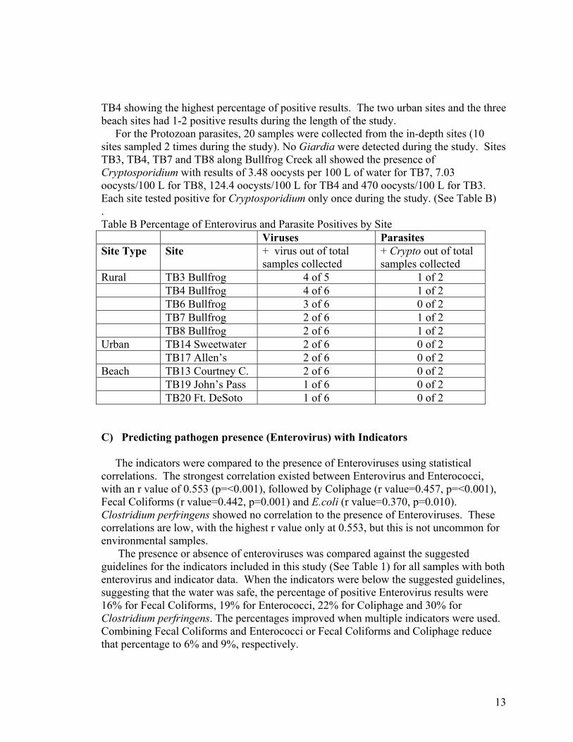
TB4 showing the highest percentage of positive results. The two urban sites and the three beach sites had 1-2 positive results during the length of the study. For the Protozoan parasites, 20 samples were collected from the in-depth sites (10 sites sampled 2 times during the study). No Giardia were detected during the study. Sites TB3, TB4, TB7 and TB8 along Bullfrog Creek all showed the presence of Cryptosporidium with results of 3.48 oocysts per 100 L of water for TB7, 7.03 oocysts/100 L for TB8, 124.4 oocysts/100 L for TB4 and 470 oocysts/100 L for TB3. Each site tested positive for Cryptosporidium only once during the study. (See Table B) . Table B Percentage of Enterovirus and Parasite Positives by Site Viruses Parasites Site Type Site + virus out of total

samples collected + Crypto out of total samples collected

Rural TB3 Bullfrog 4 of 5 1 of 2 TB4 Bullfrog 4 of 6 1 of 2 TB6 Bullfrog 3 of 6 0 of 2 TB7 Bullfrog 2 of 6 1 of 2 TB8 Bullfrog 2 of 6 1 of 2 Urban TB14 Sweetwater 2 of 6 0 of 2 TB17 Allen’s 2 of 6 0 of 2 Beach TB13 Courtney C. 2 of 6 0 of 2 TB19 John’s Pass 1 of 6 0 of 2 TB20 Ft. DeSoto 1 of 6 0 of 2 C) Predicting pathogen presence (Enterovirus) with Indicators The indicators were compared to the presence of Enteroviruses using statistical correlations. The strongest correlation existed between Enterovirus and Enterococci, with an r value of 0.553 (p=<0.001), followed by Coliphage (r value=0.457, p=<0.001), Fecal Coliforms (r value=0.442, p=0.001) and E.coli (r value=0.370, p=0.010). Clostridium perfringens showed no correlation to the presence of Enteroviruses. These correlations are low, with the highest r value only at 0.553, but this is not uncommon for environmental samples. The presence or absence of enteroviruses was compared against the suggested guidelines for the indicators included in this study (See Table 1) for all samples with both enterovirus and indicator data. When the indicators were below the suggested guidelines, suggesting that the water was safe, the percentage of positive Enterovirus results were 16% for Fecal Coliforms, 19% for Enterococci, 22% for Coliphage and 30% for Clostridium perfringens. The percentages improved when multiple indicators were used. Combining Fecal Coliforms and Enterococci or Fecal Coliforms and Coliphage reduce that percentage to 6% and 9%, respectively.

14

D) Fecal Coliform Source Tracking The most striking finding of this study was the extent to which wild animals dominate as a source of fecal coliforms and E.coli, in 73.6% of all samples, the majority of isolates were identified as nonhuman. All of the source-specific methods used in the study indicate that human pollution is significantly impacting the Bullfrog Creek Watershed. The consistent impact from human sources is less clear at the Pinellas county sites, although there were days when “spikes” of human isolates dominated the sites. The percentage of isolates identified as human by antibiotic resistance analysis was significantly correlated with enterovirus counts, but the percentage of isolates identified as human by ribotyping was not significantly correlated with enterovirus counts. This discrepancy points to the need for including the fingerprints of more isolates from known, local sources in the respective databases.

E) Climate and Indicators The Fall peak in fecal indicator levels corresponded to the end of the rainy season, however, the Spring peak could not be linked to rainfall or stream flow parameters. A lag time beyond 30 days existed when rainfall was compared to the indicators, but localized peaks associated with rainfall events may still occur within individual watersheds. Total rainfall rather than average rainfall was better than stream flow for predicting indicator level peaks overall. For Enterococci, the 7 day total rainfall value was useful, but for coliphage, the 3 day total was better perhaps because of the decreased survival of this indicator in warm tropical waters. Average rainfall for beach sites was useful only when looking widely at the Bay, not for the individual sites. Enterococci compared to the 10 day total rainfall value was the only useful indicator correlation at the beach sites. Negative correlations to rainfall and stream flow suggest that in some watersheds dilution due to increased rainfall and stream flow will actually decrease the number of phage and Clostridium. Both coliphage and Clostridium were found in low numbers compared to the other indicators. Sources are more likely to be related to feces compared to coliforms and Enterococci, which might have a soil or vegetative source. And while Clostridium could accumulate in sediments and does survive for extended periods of time, the low concentrations make it susceptible to non-detects when fresh water increases. Binary Logistic Regressions were used to determine the relationship between rainfall, stream flow and the presence of Enterovirus. A slightly significant logistic regression result occurred within the beach site grouping between the 7 day average rainfall values and the presence of Enterovirus, resulting in a 64.3% concordant percentage, 30.4% discordant percentage and a 5.4% tie. Salinity and Enterovirus in this same beach grouping resulted in a concordant percentage of 69.6%, 26.8% discordant percentage and a 3.6% tie. No other significant relationship was found between the climate factors used in the study, and the presence or absence of Enterovirus. The virus data set for this study is small, however, and a more intensive virus sampling regime may be needed for a more

15

accurate statistical analysis of climate factors and their contribution to virus water quality on the beaches. V. Recommendations What indicators are appropriate for Tampa Bay? • The use of two indicators, both the fecal coliform bacteria and enterococci on a

routine basis is warranted based on the results of this study. E.coli appears to be of little added value in either marine or fresh waters.

• Source tracking using multiple antibiotic resistance for fecal coliform bacteria should be included and a large catalog and repository for Tampa Bay should be built and supported.

• Coliphage should be added as a third indicator in areas with fresh water inputs during the study of storm events on water quality.

• Clostridium perfringens and Bacteroides phage, while indicative of fecal pollution, only have limited added value as alternative indicators.

• Clostridium may be useful during one-time sanitary surveys. • Bacteriodes will be useful in studying wastewater facilities (disinfected wastewater)

and septic tank inputs into common warm marine waters. • Biological Source Tracking is a very useful tool, and a large database for Tampa Bay

should be built and supported. The continued use of fecal coliform bacteria is supported but only with the addition of enterococci, as well as characterization of the types of fecal coliform bacteria found using the source tracking techniques. Coliphage as a third indicator should be added during specialized surveys. This approach will be useful in demonstrating risk, seasonal variability, sources and the data can be used to make both short-term and long-term management decisions on the watershed. What levels are appropriate for Tampa Bay? • The 104 CFU single sample level and geometric mean of 35 CFU associated with

Enterococci is partially supported by this study for the fresh water tributaries. However the 200 and 800 CFU for the fecal coliform bacteria are not and may be too stringent. A set of values for the fecal coliform bacteria can not be supported at this time.

• A greater database is needed at the contrasting beaches to make recommendations for beach water quality monitoring and levels.

Is pathogen monitoring warranted? • Viruses have been the group of pathogens which have shown the most value in

marine waters as a benchmark to compare to the indicators representing human health risks.

16

• Risk assessment models suggest that the likelihood of becoming ill is 1/1000 to 1/10,000 if ingesting water at the levels recorded on the beaches from a single swimming event. In order to further define this risk, virus testing is warranted, as a part of any particular beach study.

• Enteroviruses were found in Tampa Bay sites in 39% (23 out of 59 samples) of the samples tested, but at 100% of the sites tested. In other words, at least one positive result occurred at every site tested at some time during the study.

What other information is needed to move into Phase II Healthy Beaches? • A more detailed study directly on the beaches is needed. • Specifically working with a transport model, a temporal and spatial study is needed,

this can be accomplished using indicators. The current data set could be used to support an initial study, however more data are needed on the beaches.

Are the data and recommendations for Tampa Bay useful for a State-wide program? • Yes, state, local and private agencies involved in water quality studies (wastewater,

stromwater, septage etc), should move immediately to monitoring for both enterococci and fecal coliform bacteria as well as contributing to a state-wide database on the characterization of “source-tracking” isolates. Virus testing should be built into specialized studies.

Perspective and Future Directions: Healthy Beaches Phase II and beyond Because most pathogens are host-specific, the goal of this study has been to access the risk of human disease by measuring pollutants of human origin. However, a great deal of additional work remains in order to protect public health and enhance the environment, including: • Modeling of conditions that determine pollution events to provide ways to predict,

avoid and mitigate. Healthy Beaches Phase II has been proposed to address modeling and risk assessment. (Proposal is included in Appendix XII)

• Development of technology and methods such as biosensors to enable the rapid measurement of indicators or actual pathogens.

• Better understanding and response to waterborne diseases not necessarily of human origin, such as those that cause wound infections, animal parasites such as Giardia and Cryptosporidium, organisms from animal waste (e.g. E.coli 0157:H7), and natural organisms such as Vibrio vulnificus and harmful algal blooms.

• Development of a comprehensive database of Enterococci and Fecal Coliforms for use in biological source tracking, and development of methods to quickly perform the analysis locally.

• Increase efforts to eliminate or reduce identified causes of pollution, such as septic tanks, leaking sewer collections systems, failing lift stations, provision of sanitary facilities at beaches, and selected sources of animal pollution.

17

• Develop statutes, guidelines, methods and education programs so that the public will be aware of risks and take action accordingly as it is not possible to obtain a natural environment that is entirely risk free.

• Undertake a risk assessment investigation specific to warm climates areas, including epidemiological methods, to quantify the relationship between exposure to various concentrations of pathogens and the associated risk of acquiring disease.

19

I. Introduction Tampa Bay is located on the west central coast of Florida, opening to the Gulf of Mexico. This is a shallow subtropical estuary, one of the largest in the southeastern U.S. It is valued for its ecosystem, fisheries, recreational uses and as a port. The drainage basin is approximately 2300 square miles and includes 9 major and 76 minor sub-basins. The major tributaries in the Bay are the Hillsborough, Alafia, Little Manatee and Manatee Rivers, while minor systems include Alligator Creek, Joe’s Creek (Pinellas County), Rocky Creek, Double Branch Creek, Sweetwater Creek (northwest Hillsborough County), Tampa Bypass Canal, Delaney Creek, Bullfrog Creek (central and south Hillsborough County), and Frog Creek (Manatee County). Freshwater inputs are highly significant to the Bay and are associated with rainfall, with about 60% of the annual precipitation occurring from June to September. Along with this freshwater input is the input of contaminants originating from point and non-point sources. The estimated population in Florida by the year 2010 is 16 million people. Growth in the counties around Tampa Bay has been significant (about 1.8 million live around the Bay) and it is estimated that Pinellas, Hillsborough and Manatee will gain as many as 500,000 people in the next 10 to 15 years. Increased wastewater originating from treatment plants and septic tanks as well as increased biosolids will need to be managed. Increased urbanization has and will continue to alter the watershed as well as the freshwater flows to the Bay. Non-point source loading rates for nitrogen, phosphorous, metals, BOD and suspended solids have been estimated with current, and changes to, land use, however, more recent microbial contaminants have been identified as high priority risk to waters in coastal communities. In particular, public health issues have been highlighted by the Clean Water Initiative as a result of poor environmental conditions in coastal waters due to increased population growth and urbanization. Clean beaches and the recreational activities associated with them form the backbone of the tourist industry in the Tampa Bay region. Water quality at beaches ranges from excellent (i.e. most of the Gulf beaches, seldom closed due to water quality) to moderate (beaches on Tampa Bay and inland waterways that are periodically closed) to poor (lakes and other freshwater environments which have been permanently closed). The moderate quality beaches of particular interest (having received media attention associated with closures) include Fred Howard Park in Tarpon Springs, beaches along the Courtney Campbell and Gandy Causeways, and North Shore Beach in St. Petersburg. Bodies of water permanently closed to swimming include Brooker Creek Park at Lake Tarpon, the Boy Scout Camp at Lake Chautaqua and Wall Springs. The latter is of particular interest because it represents a growing problem with springs in Florida, that is, deterioration of groundwater quality. Risks to swimmers using polluted beaches has been a major issue associated with the setting of ambient water quality standards and discharge limits to recreational sites. Public health concerns in recreational waters in the tropics and subtropics differ from those of cooler waters. Prevention of disease depends on the use of appropriate fecal

20

indicators. However, the finding that the most widely used fecal contamination indicator, fecal coliforms and more specifically E. coli, grow naturally on vegetation in warm climates clearly brings into question whether these or other indicators developed for temperate climates are applicable in Florida and other southeastern areas. (Fujioka et al, 1999) In recent years, total and fecal coliform bacterial indicators have not been able to consistently indicate the persistence of pathogens, especially viruses in surface waters. F-specific RNA coliphage, enterococci and Clostridium perfringens have been suggested as better indicators of fecal contamination and public health risks. Table 1 outlines some advantages and disadvantage of these traditional and alternative indicators. Table 1 Indicators of fecal contamination Indicator Advantage Disadvantage Potential Use for

Tropical Waters Fecal Coliforms Historical database.

Good relationship to rainfall.

Found to be ubiquitous in water and other environments, no relationship to pathogens. Variability in levels is great, regardless of pollution source.

Useful for source tracking using antibiotic resistant markers. Resolution to the source genus level (dog, human, cow, bird and soil).

E.coli Is a potential pathogen, indicates potentially greater risk, and due to liability cannot be ignored

Most of the E.coli is harmless, can have a variety of sources including soil.

Applicable to biosensors for pathogen detection. (eg. 0157:H7) Ribotyping can be used to differentiate animal and human sources; correlates well with detection of human sources of pollutants in fresh/ low salinity waters.

Enterococci Found in large numbers relative to some alternative indicators, good correlation with enteric viruses

Has both environmental and fecal sources. Its common occurrence in tropical soils is not well known.

Generally a good fecal indicator for both fresh and marine water.

21

Clostridium perfringens

In low dilution areas, with waterways which are estuarine, less influence by salinity

Low levels. Little relationship to pathogens.

Limited application, good in transects in watersheds from fresh to saline.

Coliphage Appear to be a better indicator in fresh water systems, only in one watershed could the phage be related to enteric viruses.

Survives very poorly in warm marine waters.

Indication of fresh water inputs; can be typed for animal/human distinction.

Bacteroides fragilis phage

Survives well in warm marine waters. Can identify human impact within 48 hours.

Found in low numbers in wastes. Appears susceptible to chlorination process in wastewater plants.

In areas of low dilution, can indicate human septic wastes, as not found in treated-disinfected sewage;applicable to warm marine waters.

a) Water Quality Studies in Florida Our laboratories have been involved in the study of microbial quality of Florida waters since 1992. (Paul et al., 1995) Studies have been conducted in the Florida Keys and more recently along the Pithlachascotee River, in Homosassa Springs, Satasota County along the Phillippi Creek and in Charlotte Harbor for microbial contaminants associated with public health risks (Rose et al.,1995, Lipp et al.,2000:2000a, Griffin et al.,1999-2000). Both traditional and alternative indicators in addition to pathogen monitoring for viruses and parasites have been used in these studies. Fecal contamination associated with non-point sources (septic tanks ands storm water) all along the Phillippi Creek was evident based on the use of four indicators of pollution (fecal coliform bacteria, coliphage, Enterococci and Clostridium perfringens). The water quality could not meet Florida State standards or Federal guidelines for safe swimming. The Enteric protozoa, Cryptosporidium and Giardia, were detected, but more significantly, human viruses were detected in 91% of the sites sampled. In comparing indicator organisms against pathogens, 64.7% of the samples with pathogens had >100 cfu/100 mL for fecal coliforms and levels of bacteria were highest during the rainy season and at areas with the greatest density of septic tanks. In contrast, Clostridium and coliphage were found at lower numbers. In 41% of the samples

22

containing pathogens, these indicators were at non-detectable levels. Enterococci proved to be the most accurate indicator of pathogen presence, as 76% of the samples containing pathogens contained >35 cfu/100 mL. All four indicators, however, could be used in cluster analysis to pinpoint high pollution waterways. (Lipp et al.,2000) Studies along the Pithlachascotee River showed significantly less contamination compared to Phillippi Creek using similar bacterial and viral indicators (values were on average 2 to 10 times lower). No protozoa were detected. Peaks of contaminants were associated with rainfall events, and in this study, subsurface contamination was indicated in the upper reaches and most urbanized sites of the river. Management of septic tanks and storm waters contributed to an improved water quality compared to areas like Phillippi Creek. Water quality in Charlotte Harbor was studied for one year primarily at sites with salinities greater than 15 ppt. (Lipp et al.,2000a) All four fecal indicators (see above) were correlated with stream flows from the Myakka and Peace Rivers. Numbers of Enterococci were highly correlated with the freshwater flows, and Enterococci proved to be a good indicator of virus contamination, with 87% of virus-positive samples containing Enterococcus levels of >35cfu/100 mL El Niño related rain events in November, December, January and February were associated with human virus detection and increased virus indicators (coliphage) at near shore and off shore sites. In this case, the coliphage accurately predicted the presence of human viruses at levels greater than 100 pfu/100 mL. In addition, the indicators were shown to accumulate in the sediments. Levels were 10 to 100x higher than in the water column with the exception of the coliphage (which may be due to the rapid die-off). Human enteric viruses were detected by RT-PCR in 95% of the canals in the Florida Keys influenced by septic systems (Griffin et al.,1999). Clostridium was detected in 63% of the sites, however, concentrations were very low. Only once was greater than 26 cfu/100 mL detected. Coliphage were detected in only 10% of the sites, while approximately 79% of the sites were positive for fecal coliforms, E.coli, and Enterococci. Forty seven percent of the sites had Enterococci levels greater than 35 cfu/100 mL, and 21% of the sites had fecal coliforms >200 cfu/100 mL. E.coli constituted 13-99% of the fecal coliform population at each site. Increasingly, in later studies (unpublished data), no culturable viruses were detected until the winter months. This finding can be attributed to considerably cooler water temperatures, since coliphage were found to die off rapidly in warm saline waters such as those found in the Florida Keys. The use of F+ specific coliphage was applied in Homosassa Springs, Florida to identify the impact of an animal park on the water quality (Griffin et al., 2000). Rainfall significantly influenced the levels of all four indicators. Fecal coliforms were found throughout the water way at around 100 cfu/100 mL, but were higher (~3000 cfu/100 mL) at areas directly influenced by discharges from the animal holding pens. Clostridium and enterococci were also elevated in these areas. Coliphage were

23

consistently recovered from this cool, freshwater system. A coliphage enrichment procedure followed by genotyping indicated that animals were the likely source of the contamination. To date, extensive investigations into the range of microbial contaminants, the sources and public health risks have not been undertaken in Tampa Bay, however, studies on fecal coliform bacteria showed that Bullfrog Creek and Delaney Creek were the most heavily contaminated, followed by the Lake Thonotosassa tributaries. These levels were in exceedance of the Florida standards for recreational waters and in violation of Florida State Standards for Safe Swimming (200CFU/100ml). (EPC-Hillsborough County Report 1995-1997) b) Goals of Healthy Beaches Tampa Bay The goals of this study were: 3) To determine appropriate indicators for microbiological water quality for recreational



This study examined alternative pollution indicators and their association with environmental variables (salinity, rainfall, stream flow) in key basins. The study examined the water quality of near shore to off shore sites in the Bay, tributaries, beach sites, estuarine sites and freshwater sites along with uses and sources of contamination. These data are to be used to better communicate the potential public health risks for recreation in Tampa Bay and for improved monitoring, remediation and management programs. The final goal of this project was to form the baseline for other studies and help to develop a long-term strategy for addressing or enhancing Florida water quality. The specific tasks included: • An historical literature review and summary of existing studies on fecal indicators in

Tampa Bay. • A survey of Tampa Bay and area beaches for fecal indicators including coliforms, E.

coli, coliphage, Bacteroides fragilis phage, Clostridium and Enterococci. • A study of antibiotic resistance markers, delineating areas of human versus animal

wastes. • A study of the occurrence of human pathogens (enteric viruses, Cryptosporidium and

Giardia) to assess the potential public health risks. • Development of data bases for incorporation into water quality hydrodynamic

modeling for evaluating ecosystems and public health. • Discussion of strategies for the future to meet the long term goals for Healthy

Beaches Tampa Bay and the State of Florida • Meetings with an Advisory committee that assisted with review, communication and

strategy development.

24

II. Approaches a) Advisory Council

An advisory committee was set up headed by Ms. Holly Greening of the Tampa Bay Estuary Program to provide assistance in site selection, aid in community awareness, and to review the results of the study.

b) Literature Review

An retrospective analysis of the historical fecal coliform data from Tampa Bay was performed by Dr. Erin Lipp at USF. The report is included in Appendix I.

c) Sampling sites and watershed descriptions Twenty-two sites were chosen in Tampa Bay for this study with the assistance of the advisory council. The final choices were based on watershed representation, areas of concern in regard to pollution, accessibility and previously sampled sites. Table 2 gives an overview of the sites selected, and Figure 1 shows their location along Tampa Bay. Eleven sites of primarily rural or suburban land use were chosen in Hillsborough and Manatee counties. Six sites were located in highly urban areas (mainly in Pinellas county with the exception of Sweetwater Creek -TB14 and the Hillsborough River -TB12), and 4 beach sites were chosen to represent several different beach types, including urban (TB13 Courtney Campbell Causeway beach), heavy boat use (TB19 John’s Pass), recreational site in rural area (TB20 North Beach, Ft. DeSoto) and pristine unpopulated beach (TB16 Honeymoon Island). A detailed listing of the sampling sites and directions for each are found in Appendix II, and the GIS locations of each of these sites are in Appendix III. Tampa Bay can be divided into five areas, which include four distinct watersheds in Hillsborough county and the peninsula of Pinellas county. Several small sub-basins are located around the Bay as well. The Alafia watershed was represented by sites TB2 and TB5, the Little Manatee by sites TB9 and TB10, the Manatee watershed by site TB11 and the Hillsborough watershed by site TB12. The Bullfrog Creek sub-basin was chosen for in-depth monitoring due to the history of heavy pollution in the system. Sites TB3, TB4, TB6, TB7 and TB8 were located along this system (See Figure 1a). The Delaney Creek sub-basin was represented by site TB1. The remaining sites were located in Pinellas county, which cannot be divided into distinct watersheds, but is rather several non-continuous creek and wetland systems. A detailed description of the major watersheds can be found in Appendix IV.

25

Table 2 Sampling Site Overview Watershed Description

Site ID Watershed Site description

Rural TB1 Delaney Sub-basin system in central Hills. Co. TB2 Alafia Mouth of Alafia River TB3 Bullfrog Sub-basin system in central Hills. Co. TB4 Bullfrog Further inland site along Creek TB5 Alafia Inland on Alafia River TB6 Bullfrog Junction of Little and Big Bullfrog TB7 Bullfrog Little Bullfrog headwater TB8 Bullfrog Big Bullfrog headwater TB9 L. Manatee Inland site along Little Manatee River TB10 L. Manatee Mouth of Little Manatee River TB11 Manatee Mouth of Manatee River Urban TB12 Hillsb. Downtown Tampa, Univ of Tampa TB14 Sweetwater Sub-basin, Highly developed area TB15 Pinellas Lake Tarpon Bypass Canal TB17 Pinellas Allen’s Creek ,US 19 in Clearwater TB18 Pinellas Joe’s Creek and Cross Bayou, St. Pete TB21 Pinellas Salt Creek south of downtown St.Pete Beach TB13 Pinellas Clearwater /Courtney C. Causeway TB16 Pinellas Honeymoon Island, upper beach TB19 Pinellas John’s Pass, Inter coastal, boat traffic TB20 Pinellas North Beach, Ft. DeSoto, inside beach Control TB22 Bay Midwater, center of Tampa Bay

26

Figure 1 Tampa Bay Sampling Sites

27

Figure 1a Bullfrog Creek Sampling Sites in Detail

28

d) Sampling Schedule Each site was sampled monthly for a period of approximately one year for traditional and alternative fecal indicators, which included Fecal Coliforms, E.coli, Enterococci, Clostridium perfringens and Coliphage. Physical parameters were measured at the time of sampling as well, and included temperature, pH, turbidity and salinity. A list of the physical measurements, as well as the date and time of each sample, is found in Appendix V. Out of the 22 total sites, 10 were chosen for in-depth testing (including antibiotic resistance analysis, ribotyping of E. coli isolates, enterovirus detection and Bacteroides fragilis phage assay). These sites were monitored 6 times throughout the study. The sites chosen for in-depth study in Hillsborough County include all sites along Bullfrog Creek: TB3, TB4, TB6, TB7, TB8. In Pinellas County, the sites include TB13 Courtney Campbell Causeway, TB14 Sweetwater Creek, TB17 Allen’s Creek, TB19 John’s Pass Beach and TB20 North Beach, Ft. DeSoto. Table 3 gives an overview of the sampling strategy for the study. Table 3 Overview of Sampling Strategy Sampling sites Number of samplings in study and tests performed Indicators (9-12) In-depth tests (6) Parasites (2) TB1 Delaney Creek X TB2 Alafia River X TB5Alafia River X TB9 Little Manatee River X TB10 Little Manatee River X TB11 Manatee River X TB12 Hillsborough River X TB15 Lake Tarpon Canal X TB18 Joe’s Creek X TB21 Salt Creek X TB22 Control Site X TB3 Bullfrog Creek X X X TB4 X X X TB6 X X X TB7 X X X TB8 X X X TB13 Courtney Campbell X X X TB14 Sweetwater Creek X X X TB16 Honeymoon Island X X X TB17 Allen’s Creek X X X TB19 John’s Pass X X X TB20 Ft. DeSoto X X X

29

e) Materials and Methods Sample Collection Grab samples were collected in sterile 1 L plastic bottles and placed on ice for transportation to the lab. Samples were processed within 8 hours of collection. Fecal Indicators For each bacterial indicator assayed, volumes of the water sample were filtered through a 0.45µm pore size membrane filter (Osmonics) using a 47mm Gelman filter funnel fitted to a vacuum manifold. Sample volumes were determined by the fecal contamination level at each site. The filters were then placed on the appropriate media as described below for each individual bacterial indicator assay. Fecal coliforms were enumerated according to the Standard Methods for Examination of Water and Wastewater, APHA, 1989 (71). Water samples were filtered as described above and placed on mFC agar plates (Difco). Plates were then incubated for 18 to 24 hours at 44.5oC in a water bath. The dark blue colonies were counted as fecal coliforms. Enterococci were enumerated using Method 1600, USEPA. (72) Water samples were filtered as described above. The filters were placed on mEI agar plates (Difco) and incubated for 18 to 24 hours at 41 oC. Those colonies exhibiting a blue halo were counted as enterococci. E. coli were enumerated by taking those plates positive for fecal coliforms, transferring the membrane filter to EC with MUG media (Difco), and incubating for an additional 24 hours at 370C. Colonies that fluoresced under UV light were counted as E. coli. and isolated for ribotyping and antibiotic resistance assessment for source identification. C. perfringens were enumerated by filtering water samples as described above. The filter were then placed on mCP agar plates (acumedia- Baltimore, Maryland) and incubated anaerobically in GasPak jars (BBL GasPak, Becton Dickinson) for 18 to 24 hours at 450C. Yellow colonies that turned pink or red when exposed to ammonium hydroxide fumes were counted as C. perfringens. Coliphage were enumerated according to the Standard Methods for Examination of Water and Wastewater, APHA, 1989. A 1ml aliquot of the water sample was added to a 1 ml aliquot of a log phase E. coli host bacterial culture in a tube of melted soft TSA agar and overlayed onto a TSA plate. The agar was allowed to solidify, and the plate was incubated for 18 to 24 hours at 370C. Each sample was assayed using 10 replicate plates. Phage concentration of the samples were calculated by using the number of plaques that appeared on the bacterial lawn of each plate. Culturable Enteroviruses Concentrated water samples from absorption/elution using the filterite filter were prefiltered through a 0.2 µm filter (25mm, Corning) then stored at -700C (Standard Methods, 1989; Jiang et al., 1992). The samples were then quickly melted in a 370C water bath before inoculation onto cells and kept on ice during the processing. One milliliter of sample was inoculated onto each of a total of twenty 25mm2 bottles with a Buffalo green monkey (BGM) kidney cell monolayer without cell culture media. After the bottles with the sample were incubated with the cell side down at 370C for two hours,

30

maintenance medium (E-MEN with 5% fetal calf serum) was added to each bottle. The bottles were incubated at 370C for two weeks and evaluated daily for cell destruction caused by viruses known as cytopathic effects (CPE). Both positive and negative samples were frozen at -700C and thawed at 370C before being transferred (1ml of each) to a 13x100mm tube with a new BGM monolayer. The tubes were incubated at 370C for two more weeks and examined for CPE each day (Standard Methods for Examination of Water and Wastewater, 1989). Protozoan Analysis Samples were processed and assayed using filtration and immunofluorescence microscopy techniques (Federal Register/Vol. 59, No. 28/February 10, 1994 Appendix C to Subpart M – Proposed ICR Protozoan Method for Detecting Giardia cysts and Cryptosporidium oocysts in Water by Fluorescent Antibody Technique. D-19 Proposal P 229, Proposed Test Method for Giardia cysts and Cryptosporidium oocysts in Low Turbidity Water by a Flourescent Antibody Procedure. 1992. Annual Book of ASTM Standards, ASTM, Philadelphia, PA. Section 9711, Pathogenic Protozoa, Proposed Method for Giardia and Cryptosporidium spp. 1993. Standard Methods for the Examination of Water and Wastewater, 18th ed. Supplement, APHA, AWWA, WEF, Washington , DC.) Between 160 and 400 L (35 to 630 gallons) were collected from the 10 sites. Samples were collected by filtration through a 1.0 µm 10 inch yarn wound filter cartridge. Volumes were monitored by attached flow meters. After collection, the filters were placed on ice for transport to the USF lab, then cut apart and washed to collect the material from the filter and recover protozoan cysts and oocysts. Final washed volume was then centrifuged to a concentrated pellet representing the initial volume of water collected. The final concentrates were examined using immunofluorescence microscopy with monoclonal antibodies (Mab) specific to the oocyst and cyst wall which are labeled with a specific stain. Equivalent volumes from the concentrates examined under the microscope were calculated and the concentrations of cysts and oocysts per 100 L were determined. Antibiotic Resistance Analysis Antibiotic Resistance Analysis (ARA) – E.coli isolates were picked from filters incubated with mFC medium (see Fecal Coliforms). Isolated colonies were transferred individually to microtitre dish wells containing EC broth. Microtitre dishes were incubated for 24 hours at 44.50 C. The antibiotic resistance pattern (ARP) of each isolate was defined by the growth on at least eight antibiotics at four concentrations each, which was accomplished by replica plating isolates from the microtitre dishes to TSA plates which were each amended with one antibiotic. The antibiotic used were amoxicillin, cephalothin, erythromycin, ofloxacin, tetracycline, gentamicin, chlortetracyline and moxalactam. The ARP of each isolate was compared to ARP’s of isolates from known sources (cattle, wild animals, human, etc.) by discriminant analysis. Discriminant analysis assigned each isolate to a source category based on the similarity of the isolate’s ARP to those from known sources in the database.

31

Ribotyping Ribotyping of E.coli isolates was accomplished by the method of Parveen et al (1997). Chromosomal DNA was extracted from E.coli isolates and digested with Hind/III. Fragments were separated by agarose electrophoresis. The cDNA from the E.coli 16S rDNA was labeled with digoxigenin-dUTP and used as probes. E.coli ribotype profiles were then compared to those of Dr. George Lukasik’s known source library by discriminant analysis. This library was developed in the laboratory of Dr. Mark Tamplin, formerly of University of Florida, now with the USDA.

32

III. Results A) Sampling Summary

Sampling began in June 1999 and ended in August 2000. The total sampling sites (22) were divided into two groups, and a group was sampled every other week. The control site was sampled according to the Environmental Protection Commission of Hillsborough County’s monthly sampling schedule, and brought to the University of South Florida, St. Petersburg campus on the day of collection. Sampling was extended beyond the initial 12 month period to compensate for missed specimens due to weather or scheduling conflicts. A total of 60 Enterovirus samples were collected and analyzed for the 10 in-depth study sites over the 15 month sampling period, and 20 total parasite samples were collected and analyzed for the 10 in-depth sites as well, one set every 6 months during the study. The following table (Table 4) gives the fecal indicator guidelines and levels used for the comparison of the data in this study. For the individual sampling results, the single sample guideline was used for Fecal Coliforms and Enterococci. No single sample guidelines are given for E.coli, Clostridium perfringens and Coliphage. In these cases, the geometric mean guideline was used. For the site to site comparisons, the geometric mean of all the results obtained throughout the study were used and compared to the geometric mean guidelines given.

Table 4 Indicator Guidelines used in this study Fecal Coliforms EPA and the state of Florida recommended guidelines for a single






33

B) Results of Traditional and Alternative Indicators The sampling sites were divided up into the categories of rural (which included suburban areas), urban and beach sites. The arithmetic and geometric averages for each individual indicator at each sampling site were calculated. Less than values, or those values that fell below the limit of detection for that indicator, were changed to zeros to calculate the averages. Tables with each individual sampling and the results of the indicator data can be found in Appendix VI. Below are summary tables (Tables 4 through 8) for each indicator (Fecal Coliforms, E.coli, Enterococci, Clostridium perfringens and Coliphage). The sites are divided into rural, urban and beach sites, with the control site at the bottom of the table. The site designations are given, and the total number of samples is listed under the “n” column. The range is given to show the lowest and highest indicator result seen in the course of the study. The percent Positive column is based on the number of specimens in which the indicator was detected at any level above the detection limit. The last two columns are the arithmetic and geometric mean of the indicator for the entire period of the study. For Table 5, Fecal coliforms, the results ranged from <1 cfu/100 mL at the control site to 174,900 cfu/100 mL at TB4 Bullfrog Creek. In the rural sites, the percentage of positive results was generally 100%, with slightly lower percentages for the urban sites, and lower still for the beach sites. The only exception to this was TB13 Courtney Campbell Causeway beach, with fecal coliforms present 100% of the time during the sampling period. The arithmetic mean ranged from 0.4 cfu/100 mL at the control site to 22,687 cfu/100 mL at TB4 Bullfrog Creek, and the geometric mean ranged from 0.2 cfu/100 mL to 5032 cfu/100 mL at the control site and TB4 Bullfrog Creek, respectively In Table 6 for E.coli, results are very similar to the fecal coliforms trends as described above. Enterococci in Table 7 ranged from <2 and <4 cfu/100 mL at several sites (including 3 out of the 4 beach sites) to 135,650 cfu/100 mL at TB4 Bullfrog Creek. In both the rural and urban sites, Enterococci was found generally 100% of the time, but only 38 to 92% of the time at the beach sites. The arithmetic mean for enterococci ranged from 0.3 cfu/100 mL at the control site to 14,520 cfu/100 mL at TB4 Bullfrog Creek, and the geometric mean ranged from 0.2 cfu/100 mL at the control site to 3009 cfu/100 mL at TB4 Bullfrog Creek. For Table 8, Clostridium perfringens, the results ranged from below the detection limit for all sites of the study to 160 cfu/100 mL at TB4 Bullfrog Creek. Clostridium was never found 100% of the time at any site, and the higher percentages occurred in the rural sites as well as the urban sites. The percentage for the beach sites were very low with the exception of TB13 Courtney Campbell Causeway beach, in which C. perfringens was detected 58% of the time. The arithmetic mean ranged from below the detection limit for TB16 Honeymoon Island and the control site to 32.7 cfu/100 ml at TB4 Bullfrog Creek, and the geometric mean ranged from below the detection limit for TB16 Honeymoon Island and the control site to 11.3 cfu/100 mL at TB3 Bullfrog Creek. For the 4 beach sites, C.perfringens was only found consistently at TB13 Courtney Campbell Causeway Beach, the most urban-located beach in the study. C.perfringens only occurred once at

34

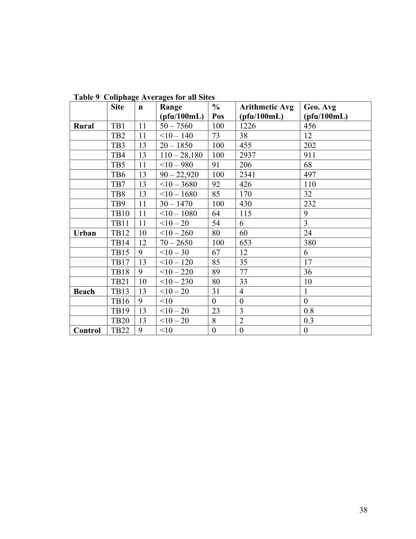
TB20 North Beach, twice at TB19 John’s Pass, and was never detected at TB16 Honeymoon Island. For the final indicator, Coliphage, Table 9 shows the results ranged from below the detection limit for most of the sampling sites to 28,180 pfu/100 mL for TB4 Bullfrog Creek. The percentage of positive samples ranged from 54 to 100% for both the urban and rural sites, but showed very low percentages for the beach sites. Coliphage showed a similar pattern to Clostridium in regard to the beach sites. The arithmetic mean ranged from below the detection limit for TB16 Honeymoon Island and the control site to 2937 pfu/100 mL at TB4 Bullfrog Creek, and the geometric mean ranged from below the detection limit for TB16 Honeymoon Island and the control site to 911 pfu/100 mL at TB4 Bullfrog Creek. Table 5 Fecal Coliform Averages for all Sites Site n Range

(cfu/100mL) % Pos Arithmetic Avg

(cfu/100mL) Geo. Avg (cfu/100mL)

Rural TB1 12 55 - 24,450 100 3045 472 TB2 12 <10 - 7415 83 804 58 TB3 12 100 - 16,350 100 2998 913 TB4 13 550 - 174,900 100 22,687 5032 TB5 12 35 - 5300 100 1223 664 TB6 13 300 - 110,200 100 9997 1688 TB7 13 12 - 13,850 100 4057 977 TB8 13 90 - 6050 100 755 296 TB9 12 100 – 10,250 100 1510 455 TB10 12 10 – 4140 100 525 106 TB11 11 <10 – 3890 91 402 34 Urban TB12 10 <10 – 3400 90 1194 265 TB14 13 80 – 33,150 100 9421 3655 TB15 10 35 – 40,000 100 4187 298 TB17 13 <10 – 23,700 92 3377 665 TB18 10 <10 – 3115 90 501 114 TB21 11 <10 – 6100 82 1656 185 Beach TB13 13 15 – 26,900 100 3057 300 TB16 10 <4 – 4745 80 523 17 TB19 12 <10 – 13,240 83 1438 53 TB20 13 <4 – 10,900 54 1574 25 Control TB22 11 <1 - 4 18 0.4 0.2

35

Table 6 E.coli Averages for all Sites Site n Range



Rural TB1 10 50 – 24,450 100 3589 561 TB2 10 0.5 – 7415 100 831 63 TB3 11 75 – 16,350 100 2846 592 TB4 11 50 – 174,900 100 23,948 2302 TB5 10 85 – 5300 100 1250 653 TB6 11 350 – 110,200 100 10,893 1231 TB7 10 175 – 17,200 100 3617 844 TB8 10 70 – 900 100 233 214 TB9 10 45 – 10,250 100 1622 336 TB10 10 10 – 4140 100 534 87 TB11 10 <10 – 3890 90 407 19 Urban TB12 8 15 – 3200 100 768 264 TB14 11 80 – 15,100 100 3789 1378 TB15 8 45 – 235 100 111 57 TB17 12 <10 –23,700 92 2476 314 TB18 9 <10 – 3115 89 466 96 TB21 10 <10 – 5340 90 1362 222 Beach TB13 11 10 – 26,900 100 3460 231 TB16 9 <4 – 4745 78 559 16 TB19 12 <10 – 13,240 83 1400 42 TB20 12 <4 – 10,900 50 1643 26 Control TB22 7 <1 - <10 0 0 0

36

Table 7 Enterococci Averages for all Sites Site n Range



Rural TB1 12 40 –12,300 100 1542 419 TB2 12 <4 – 496 83 70 15 TB3 13 10 – 17,200 100 1609 189 TB4 13 134 – 135,650 100 14,520 3009 TB5 12 2 – 6350 100 1144 269 TB6 13 68 – 43,000 100 7738 1065 TB7 13 44 – 31,650 100 3852 745 TB8 13 42 – 17,850 100 1593 231 TB9 12 20 – 17,200 100 1962 216 TB10 12 10 – 2905 100 305 55 TB11 11 <4 – 102 82 18 7 Urban TB12 10 2 – 585 100 157 65 TB14 13 5 – 35,000 100 5779 940 TB15 10 8 – 236 100 70 37 TB17 13 14 – 720 100 205 109 TB18 10 8 – 124 100 52 33 TB21 11 <4 – 1270 82 146 19 Beach TB13 13 <10 – 600 92 123 47 TB16 10 <2 – 557 60 58 3 TB19 13 <4 – 28 77 5 3 TB20 13 <4 – 77 38 7 0.9 Control TB22 10 <4 - 1 30 0.3 0.2

37

Table 8 Clostridium perfringens Averages for all Sites Site n Range



Rural TB1 11 <4 – 32 64 7.8 3.7 TB2 11 <4 – 14 64 4.1 2.3 TB3 12 <4 – 50 83 20.8 11.3 TB4 13 <4 – 160 62 32.7 7.8 TB5 11 <4 – 46 64 9.5 3.4 TB6 13 <4 – 46 54 12.5 4.3 TB7 13 <4 – 32 77 7.9 4.0 TB8 13 <4 – 16 62 4.8 2.5 TB9 11 <4 – 16 45 3.5 1.5 TB10 11 <4 – 14 45 2.9 1.2 TB11 11 <4 – 6 45 1.2 0.7 Urban TB12 9 <4 – 22 56 4 1.7 TB14 12 <4 – 148 75 25 7.4 TB15 8 <4 – 34 75 8.4 4.1 TB17 12 <2 – 26 67 7.8 3.7 TB18 8 <2 – 30 63 11.1 4.7 TB21 9 <2 – 18 22 2.4 0.7 Beach TB13 12 <4 – 52 58 11 3.5 TB16 8 <2 - <4 0 0 0 TB19 12 <2 - <4 17 0.5 0.3 TB20 12 <2 – 10 8 0.8 0.2 Control TB22 8 <2 - <4 0 0 0

38

Table 9 Coliphage Averages for all Sites Site n Range

(pfu/100mL) % Pos

Arithmetic Avg (pfu/100mL)

Geo. Avg (pfu/100mL)

Rural TB1 11 50 – 7560 100 1226 456 TB2 11 <10 – 140 73 38 12 TB3 13 20 – 1850 100 455 202 TB4 13 110 – 28,180 100 2937 911 TB5 11 <10 – 980 91 206 68 TB6 13 90 – 22,920 100 2341 497 TB7 13 <10 – 3680 92 426 110 TB8 13 <10 – 1680 85 170 32 TB9 11 30 – 1470 100 430 232 TB10 11 <10 – 1080 64 115 9 TB11 11 <10 – 20 54 6 3 Urban TB12 10 <10 – 260 80 60 24 TB14 12 70 – 2650 100 653 380 TB15 9 <10 – 30 67 12 6 TB17 13 <10 – 120 85 35 17 TB18 9 <10 – 220 89 77 36 TB21 10 <10 – 230 80 33 10 Beach TB13 13 <10 – 20 31 4 1 TB16 9 <10 0 0 0 TB19 13 <10 – 20 23 3 0.8 TB20 13 <10 – 20 8 2 0.3 Control TB22 9 <10 0 0 0

39

Table 10 gives a summary of the individual sampling events that exceeded the suggested indicator guidelines for Fecal Coliforms, E. coli, Enterococci, Clostridium perfringens and Coliphage. For each indicator, a column is given to show the percentage of the samples that exceeded the suggested guidelines for single samples found in Table 4. For those indicators that did not have a single sample guideline (E.coli, C.perfringens and coliphage), the geometric mean guideline was used. Sites TB4 Bullfrog Creek and TB14 Sweetwater Creek consistently had high levels of indicators except for C. perfringens. Sites TB6 and TB7 along Bullfrog Creek generally had high levels of Fecal Coliforms, E.coli, Enterococci and Coliphage as well. The other sites showed less contamination, with TB17 Allen’s Creek and TB5 Alafia River showing moderate levels of indicators. Site TB1 Delaney Creek had high levels of E.coli , Enterococci and Coliphage, but low levels of Fecal Coliforms and C. perfringens. Sites TB3 Bullfrog Creek, TB17 Allen’s Creek and TB18 Joe’s Creek had the highest levels detected for C.perfringens. For the beach sites, TB13 Courtney Campbell Causeway beach had the highest levels of indicators followed by TB20 Ft. DeSoto. The control site, TB22, had indicator levels below all guidelines for the entire length of the study.

Table 10 Summary of samples exceeding the suggested single sample Indicator guidelines

Site Fecal Coliforms E.coli Enterococci C.perfingens ColiphageRural TB1 17% 90% 75% 0% 91% TB2 8% 40% 17% 27% 9% TB3 33% 82% 46% 67% 62% TB4 77% 91% 100% 23% 100% TB5 42% 90% 67% 0% 36% TB6 69% 100% 85% 0% 92% TB7 38% 100% 92% 0% 62% TB8 15% 60% 62% 0% 23% TB9 25% 60% 58% 0% 73% TB10 17% 30% 25% 18% 9% TB11 9% 10% 0% 9% 0% Urban TB12 40% 75% 40% 11% 10% TB14 85% 91% 85% 17% 75% TB15 10% 25% 20% 0% 0% TB17 54% 83% 62% 42% 8% TB18 20% 33% 10% 50% 22% TB21 27% 70% 18% 11% 10% Beach TB13 31% 55% 38% 25% 0% TB16 10% 22% 10% 0% 0% TB19 17% 25% 0% 0% 0% TB20 31% 33% 0% 8% 0% Control TB22 0% 0% 0% 0% 0%

40

C) Comparison of Sites Geometric Mean Graphs The graphs in Figures 2 through 6 show the geometric mean of each indicator. For each indicator graph, the X, or bottom, axis shows all the sampling sites for the study, and the Y, or left, axis shows the colony forming units (CFU) for the bacterial indicators and the plaque forming units (PFU) for the virus indicator coliphage per 100 mL of water. These data have not been log transformed, it is given in the actual numbers of organisms per 100 mL of water. For Figure 2 (Fecal Coliforms), sites TB1, TB3, TB4, TB5, TB6, TB7, TB8 and TB9, TB12, TB13m TB14 and TB15 and TB17 all exceed the EPA’s suggested guideline of 200 cfu/100 mL for a geometric mean result. Sites TB4 Bullfrog Creek and TB14 Sweetwater Creek are the two most contaminated in regard to fecal coliforms. In Figure 3 (E.coli), sites TB1, TB3, TB4, TB5, TB6, TB7, TB8 andTB9, TB12,TB13 and TB14, TB17 and TB21 all exceed EPA’s suggested guideline of 126 cfu/100 mL for a geometric mean result. Sites TB4 and TB6 along Bullfrog and TB 14 Sweetwater Creek have the highest averages for this indicator. For Figure 4 (Enterococci), sites TB1, TB3, TB4, TB5, TB6, TB7, TB8, TB9 and TB10, TB12, TB13, TB14 and TB15, and TB17 all exceed the suggested guideline of 104 cfu/100 mL for a geometric mean result. Sites TB4, TB6 and TB7 along Bullfrog Creek and TB14 Sweetwater Creek are the highest sites for this indicator. In Figure 5 (Clostridium perfringens), none of the sites exceed the recommended guideline (Fujioka et al 1985) for recreational water for a geometric result. Finally, in Figure 6 (Coliphage), sites TB1, TB3 , TB4, TB6, TB7, TB9 and TB14 all exceed 100 pfu/100 mL. Site TB4 Bullfrog Creek shows the highest mean level of coliphage. As previously mentioned, Fecal Coliforms, E.coli and Enterococci could be detected in almost all samples. Thirteen of the 22 sites were above the geometric suggested guideline for both E.coli and Fecal Coliforms, and 14 of the 22 sites were above the geometric suggested guideline for Enterococci. However, none of the beach sites with the exception of TB13 Courtney Campbell Causeway beach were above the fecal coliform and E.coli suggested geometric mean guidelines. The two consistently high sites for all of the indicators were the rural siteTB4 Bullfrog Creek and the urban site TB14 Sweetwater Creek. The remaining sites along Bullfrog Creek (TB3, TB6, TB7 and TB8) are the next highest sites in regards to geometric indicator means. The low sites were TB2 Alafia River, TB11 Manatee River, TB18 Joe’s Creek and TB22 Control site. The beach sites TB16 Honeymoon Island, TB19 John’s Pass and TB20 North Beach, Ft. DeSoto were also among the lowest geometric means for the indicators used, but the urban beach site, TB13 Courtney Campbell, did show a geometric mean above the recommended guideline for all indicators except C. perfringens and Coliphage. The lower levels of coliphage in this case may be due to the short survival time of the phage in warm saline waters.

Figure 2 Fecal Coliforms, Geometric Means by Site

Fecal Coliforms, Geometric Mean

0

1000

2000

3000

4000

5000

6000TB

1

TB2

TB3

TB4

TB5

TB6

TB7

TB8

TB9

TB10

TB11

TB12

TB13

TB14

TB15

TB16

TB17

TB18

TB19

TB20

TB21

TB22

Site

CFU

per

100

mL Based on 200 CFU per

100m L, geo m ean-EPA

42

Figure 3 E.coli Geometric Means by Site

E.coli, Geometric M ean

0

500

1000

1500

2000

2500TB

1

TB2

TB3

TB4

TB5

TB6

TB7

TB8

TB9

TB10

TB11

TB12

TB13

TB14

TB15

TB16

TB17

TB18

TB19

TB20

TB21

TB22

S ite

CFU

per

100

mL

Based on 126 CFU per 100m L geo m ean-EPA

43

Figure 4 Enterococci Geometric Means by Site

Enterococci, Geom etric M ean

0

500

1000

1500

2000

2500

3000

3500

TB1

TB2

TB3

TB4

TB5

TB6

TB7

TB8

TB9

TB10

TB11

TB12

TB13

TB14

TB15

TB16

TB17

TB18

TB19

TB20

TB21

TB22

S ite

CFU

per

100

mL

Based on 35 CFU per 100m L, geo m ean, EPA

44

Figure 5 Clostridium perfringens Geometric Means by Site

C.perfringens , Geometric Mean

0

5

10

15

20

25

30

35

40

45

50TB

1

TB2

TB3

TB4

TB5

TB6

TB7

TB8

TB9

TB10

TB11

TB12

TB13

TB14

TB15

TB16

TB17

TB18

TB19

TB20

TB21

TB22

Site

CFU

per

100

ml

45

Figure 6 Coliphage Geometric Means by Site

C o lip h ag e, G eo m etric M ean

0

100

200

300

400

500

600

700

800

900

1000

TB1

TB2

TB3

TB4

TB5

TB6

TB7

TB8

TB9

TB10

TB11

TB12

TB13

TB14

TB15

TB16

TB17

TB18

TB19

TB20

TB21

TB22

S ite

PFU

per

100

mL

B ased on 100 P F U per 100m L

46

Seasonal Graphs of Indicator Data The indicator values for each month of the study for each individual site are represented on a bar graph to illustrate the seasonal changes for each sampling site. For each graph, the X, or bottom, axis shows the months of the study, and the Y, or left, axis shows the colony forming units (CFU) for bacteria and the plaque forming units (PFU) for viruses per 100 mL of water. The CFU and PFU/100 mL are log transformed in order to compare the indicators on one graph. For example, the suggested guideline for fecal coliforms is 800 cfu/100 mL for a single sampling, which is equivalent to 2.9 on the log transformed scale. For Enterococci, the suggested level of 104 cfu/100 mL is equivalent to 2.0 on the log transformed scale. Fecal coliforms are represented by the first bar in the grouping, E.coli by the second bar, Enterococci by the third bar, C. perfringens by the fourth bar and Coliphage by the fifth and last bar in each grouping on the graph. Rural Sampling Sites Sampling began in June of 1999. For the rural sites TB1 through TB11 (Figures 7 to 17), peaks in indicator levels were generally seen in October 1999 and March 2000, and a reduction in indicator numbers occurred during the summer months. While high levels of indicators were found through out the year in Bullfrog Creek (TB3, TB4, TB6-TB8), similar peaks were found in Oct 1999 and March 2000. Some of the peaks only involved Fecal Coliforms and E.coli, while others involved the entire group of indicators. Urban Sampling Sites The urban sites consisted of TB12 Hillsborough River, TB14 Sweetwater Creek, TB15 Lake Tarpon, TB17 Allen’s Creek, TB18 Joe’s Creek and TB21 Salt Creek. (Figures 18 to 23) The peaks in these sites are more sporadic than previously seen in the rural sites. For TB12, peaks occurred in December 1999 and March 2000, while TB14 and TB18 only showed a peak in Dec 1999 and TB15 only in March 2000. Other isolated peaks occurred in some of the sites. All but one of the indicator peaks in the urban site grouping involved only Fecal Coliforms and E.coli. For the urban sites, indicator levels were fairly consistent through out the year, with a slight seasonal drop in the summer months occurring only at TB18 Joe’s Creek. Beach Sampling Sites The beach sites consisted of an urban beach (TB13 Courtney Campbell Causeway beach), a high boat traffic beach area (TB19 John’s Pass), a rural beach area with heavy recreational use (TB20 Ft. DeSoto) and a pristine beach with a high bird population and no swimming (TB16 Honeymoon Island). The beach at TB13 was the only beach site where all 5 indicators used in the study appeared. Peaks of Fecal coliforms and E.coli occurred in September 1999 and March 2000 at this site, with Clostridium perfringens and coliphage appearing sporadically through out the study. For TB19, peaks in the levels of fecal coliforms and E.coli occurred in September 1999, December 1999 and February 2000, with Clostridium perfringens and coliphage occurring only in the winter months. At TB20, high peaks of Fecal coliforms and E.coli were found in September and

47

December 1999, and February and March 2000. In this case, the indicators are rather sporadic and do not occur with any consistency. The last beach site, TB16, had only Fecal Coliforms, E.coli, and Enterococci occurring, with peaks in August, October and December 1999. Control Sampling Site Fecal Coliforms were only detected during July 1999, and Enterococci in August 1999, January and March 2000. These indicators occurred only in very low numbers. This site was not sampled December 1999 and June-August 2000.

48

Figure 7 Indicator Levels in TB1 Delaney Creek

TB1 Delaney Creek

0

0.5

1

1.5

2

2.5

3

3.5

4

4.5

5

5.5

6Ju

n-99

Jul-9

9

Aug

-99

Sep-

99

Oct

-99

Nov

-99

Dec

-99

Jan-

00

Feb-

00

Mar

-00

Apr

-00

May

-00

Jun-

00

Jul-0

0

Aug

-00

Date

CFU

or P

FU p

er 1

00m

L, L

og tr

ansf

orm

ed

Fecal ColiformsE.coliEnterococciC.perfringensColiphage

This site was not sampled June00 through Aug00

E.coli not performed in Sept, C.perfringens not performed in Dec

49

Figure 8 Indicator Levels in TB2 Alafia River

TB2 Alafia River

0

0.5

1

1.5

2

2.5

3

3.5

4

4.5

5

5.5

6

Jun-

99

Jul-9

9

Aug

-99

Sep-

99

Oct

-99

Nov

-99

Dec

-99

Jan-

00

Feb-

00

Mar

-00

Apr

-00

May

-00

Jun-

00

Jul-0

0

Aug

-00

Date

CFU

or P

FU p

er 1

00m

L, L

og tr

ansf

orm

ed


No sampling of this site occurred in Jun00 thru Aug00, C.perfringens and Coliphage not performed in May00

E. coli not performed in Sept99

50

Figure 9 Indicator Levels in TB3 Bullfrog Creek

TB3 Bullfrog Creek

0

0.5

1

1.5

2

2.5

3

3.5

4

4.5

5

5.5

6

Jun-

99

Jul-9

9

Aug

-99

Sep-

99

Oct

-99

Nov

-99

Dec

-99

Jan-

00

Feb-

00

Mar

-00

Apr

-00

May

-00

Jun-

00

Jul-0

0

Aug

-00

Date

CFU

or P

FU p

er 1

00m

L, L

og tr

ansf

orm

ed Fecal C oliform sE.coliEnterococciC .perfringensC oliphage

No sam pling o f th is s ite in May00 and June00

E .co li not perfo rm ed in Sept99, C . perfringens no t perfo rm ed in Dec and Jan., Feca l Co lifo rm s and E .co li not perform ed in Aug00

51


TB4 Bullfrog Creek

0

0.5

1

1.5

2

2.5

3

3.5

4

4.5

5

5.5

6Ju

n-99

Jul-9

9

Aug

-99

Sep-

99

Oct

-99

Nov

-99

Dec

-99

Jan-

00

Feb-

00

Mar

-00

Apr

-00

May

-00

Jun-

00

Jul-0

0

Aug

-00

Date

CFU

or P

FU p

er 1

00m

L, L

og tr

ansf

orm

ed


No sampling of this site in May and Jun00

E. coli not performed in Sept 99 and Aug 00

52

Figure 11 Indicator Levels in TB5 Alafia River

TB 5 Ala fia R iver

0

0.5

1

1.5

2

2.5

3

3.5

4

4.5

5

5.5

6

Jun-99

Jul-99

Aug-99

Sep-99

O ct-99

N ov-99

D ec-99

Jan-00

Feb-00

M ar-00

Apr-00

M ay-00

Jun-00

Jul-00

Aug-00

D ate

CFU

or P

FU p

er 1

00m

L, L

og tr

ansf

orm

ed F eca l C o liform sE .co liE nterococciC .perfringensC oliphage

T h is s ite was no t sam pled Jun00 th ru A ug00

E.co li no t perfo rmed in S ept99 , C .pe rfr ingens no t perfo rm ed D ec99 and M ay00, C o liphage no t perfo rm ed M ay00

53


TB6 Bullfrog Creek

0

0.5

1

1.5

2

2.5

3

3.5

4

4.5

5

5.5

Jun-

99

Jul-9

9

Aug

-99

Sep-

99

Oct

-99

Nov

-99

Dec

-99

Jan-

00

Feb-

00

Mar

-00

Apr

-00

May

-00

Jun-

00

Jul-0

0

Aug

-00

Date

CFU

or P

FU p

er 1

00m

L, L

og

tran

sfor

med


This site not sampled in May and Jun00

E.coli not performed in Sept99 and Aug00, C.perfringens not performed in Dec99

54


TB7 Bullfrog Creek

00.5

11.5

22.5

33.5

44.5

55.5

6

Jun-

99

Jul-9

9

Aug

-99

Sep-

99

Oct

-99

Nov

-99

Dec

-99

Jan-

00

Feb-

00

Mar

-00

Apr

-00

May

-00

Jun-

00

Jul-0

0

Aug

-00

Date

CFU

or P

FU p

er 1

00m

L, L

og tr

ansf

orm

edFecal Coliform sE.coliEnterococciC.perfringensColiphage

This site not sampled in May and Jun00

E.coli not performed in Sept99, Dec99 and Aug00

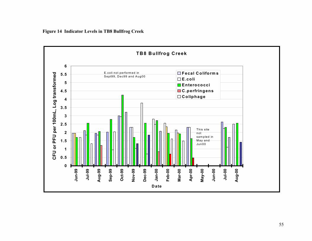
55


TB 8 B ullfrog C reek

0

0.5

1

1.5

2

2.5

3

3.5

4

4.5

5

5.5

6

Jun-

99

Jul-9

9

Aug

-99

Sep-

99

Oct

-99

Nov

-99

Dec

-99

Jan-

00

Feb-

00

Mar

-00

Apr

-00

May

-00

Jun-

00

Jul-0

0

Aug

-00

D ate

CFU

or P

FU p

er 1

00m

L, L

og tr

ansf

orm

ed F ecal C o liform sE.co liEnterococciC .perfringensC oliphage

Th is s ite no t sam p led in M ay and Jun00

E .co li no t pe rfo rm ed in S ept99 , D ec99 and A ug00

56

Figure 15 Indicator Levels in TB9 Little Manatee River

TB9 Little Manatee River

0

0.5

1

1.5

2

2.5

3

3.5

4

4.5

5

5.5

6Ju

n-99

Jul-9

9

Aug

-99

Sep-

99

Oct

-99

Nov

-99

Dec

-99

Jan-

00

Feb-

00

Mar

-00

Apr

-00

May

-00

Jun-

00

Jul-0

0

Aug

-00

Date

CFU

or P

FU p

er 1

00m

L, L

og tr

ansf

orm

ed Fecal ColiformsE.coliEnterococciC.perfringensColiphage

This site not sampled in Jun00 thru Aug00

E.coli not performed in Sept99 and May00, C.perfringens not performed in Dec99 and May00 Coliphage not

57

Figure 16 Indicator Levels in TB10 Little Manatee River

TB10 Little M anatee River

0

0.5

1

1.5

2

2.5

3

3.5

4

4.5

5

5.5

6

Jun-

99

Jul-9

9

Aug

-99

Sep-

99

Oct

-99

Nov

-99

Dec

-99

Jan-

00

Feb-

00

Mar

-00

Apr

-00

May

-00

Jun-

00

Jul-0

0

Aug

-00

Date

CFU

or P

FU p

er 1

00m

L, L

og tr

ansf

orm

ed

Fecal Coliform sE.coliEnterococciC .perfringensColiphage

This site not sampled in Jun00 thru Aug00

E.coli not performed in Sep99 and May00, C.perfringens not performed in Dec99 and May00, Coliphage not performed in May00

58

Figure 17 Indicator Levels in TB11 Manatee River

TB11 M anatee R iver

0

0.5

1

1.5

2

2.5

3

3.5

4

4.5

5

5.5

6

Jun-

99

Jul-9

9

Aug

-99

Sep-

99

Oct

-99

Nov

-99

Dec

-99

Jan-

00

Feb-

00

Mar

-00

Apr

-00

May

-00

Jun-

00

Jul-0

0

Aug

-00

D ate

CFU

or P

FU p

er 1

00m

L, L

og tr

ansf

orm

ed

Fecal C oliform sE.coliEnterococciC .perfringensC oliphage

Th is site no t sam pled in May00 th ru A ug00

E .co li no t perfo rm ed in Sept99 , C .perfringens no t perfo rm ed in Dec99

59

Figure 18 Indicator Levels in TB12 Hillsborough River

TB 12 H illsborough R iver

0

0.5

1

1.5

2

2.5

3

3.5

4

4.5

5

5.5

6

Jun-

99

Jul-9

9

Aug

-99

Sep-

99

Oct

-99

Nov

-99

Dec

-99

Jan-

00

Feb-

00

Mar

-00

Apr

-00

May

-00

Jun-

00

Jul-0

0

Aug

-00

Date

CFU

or P

FU p

er 1

00m

L, L

og tr

ansf

orm

ed Fecal Coliform sE.coliEnterococciC .perfringensColiphage

This site not sampled in Jan00, Apr00, and Jun00 thru Aug00

E.co li not performed in Dec99, C .perfringens not performed in Nov99 and M ay 00, Coliphage not performed in M ay00

60

Figure 19 Indicator Levels in TB14 Sweetwater Creek

TB14 Sweetwater Creek

0

0.5

1

1.5

2

2.5

3

3.5

4

4.5

5

5.5

6

Jun-

99

Jul-9

9

Aug

-99

Sep-

99

Oct

-99

Nov

-99

Dec

-99

Jan-

00

Feb-

00

Mar

-00

Apr

-00

May

-00

Jun-

00

Jul-0

0

Aug

-00

Date

CFU

or P

FU p

er 1

00m

L, L

og tr

ansf

orm

ed Fecal Coliforms

E.coliEnterococciC.perfringensColiphage

This site not sampled in Jan00 and Jul00

Fecal Coliforms and E.coli not performed in Aug00, C.perfringens not performed in Nov99, and

61

Figure 20 Indicator Levels in TB15 Lake Tarpon Canal

TB15 Lake Tarpon Bypass Canal

0

0.5

1

1.5

2

2.5

3

3.5

4

4.5

5

5.5

6Ju

n-99

Jul-9

9

Aug

-99

Sep-

99

Oct

-99

Nov

-99

Dec

-99

Jan-

00

Feb-

00

Mar

-00

Apr

-00

May

-00

Jun-

00

Jul-0

0

Aug

-00

Date

CFU

or P

FU p

er 1

00m

L, L

og tr

ansf

orm

ed



E.coli not performed in Mar00and May00, C.perfringens and Coliphage not performed in May00

62

Figure 21 Indicator Levels in TB17 Allen’s Creek

TB17 Allen's Creek

0

0.5

1

1.5

2

2.5

3

3.5

4

4.5

5

5.5

6

Jun-

99

Jul-9

9

Aug

-99

Sep-

99

Oct

-99

Nov

-99

Dec

-99

Jan-

00

Feb-

00

Mar

-00

Apr

-00

May

-00

Jun-

00

Jul-0

0

Aug

-00

Date

CFU

or P

FU p

er 1

00m

L, L

og tr

ansf

orm

edFecal Coliform sE.coliEnterococciC .perfringensColiphage

This site not sam pled in Jan00 and Ju l00

E.coli no t perform ed in Aug00, C .perfringens not perform ed in Nov99

63

Figure 22 Indicator Levels in TB18 Joe’s Creek

TB18 Joe's Creek/Cross Bayou

0

0.5

1

1.5

2

2.5

3

3.5

4

4.5

5

5.5

6

Jun-

99

Jul-9

9

Aug

-99

Sep-

99

Oct

-99

Nov

-99

Dec

-99

Jan-

00

Feb-

00

Mar

-00

Apr

-00

May

-00

Jun-

00

Jul-0

0

Aug

-00

Date

CFU

or P

FU p

er 1

00m

L, L

og tr

ansf

orm

ed

Fecal Coliform sE.coliEnterococciC.perfringensColiphage


E.coli not performed in May00, C.perfringens not performed in Nov99 and May00, Coliphage not performed in May00

64

Figure 23 Indicator Levels in TB21 Salt Creek

TB21 Salt Creek

0

0.5

1

1.5

2

2.5

3

3.5

4

4.5

5

5.5

6

Jun-

99

Jul-9

9

Aug

-99

Sep-

99

Oct

-99

Nov

-99

Dec

-99

Jan-

00

Feb-

00

Mar

-00

Apr

-00

May

-00

Jun-

00

Jul-0

0

Aug

-00

Date

CFU

or P

FU p

er 1

00m

L, L

og

tran

sfor

med


This site not sampled in Jan00, and Jun00 thru Aug00

C.perfringens not performed Nov99 and May00, Coliphage not performed May00

65

Figure 24 Indicator Levels in TB13 Courtney Campbell Causeway beach

TB13 Courtney Campbell Causeway Beach

0

0.5

1

1.5

2

2.5

3

3.5

4

4.5

5

5.5

6

Jun-

99

Jul-9

9

Aug

-99

Sep-

99

Oct

-99

Nov

-99

Dec

-99

Jan-

00

Feb-

00

Mar

-00

Apr

-00

May

-00

Jun-

00

Jul-0

0

Aug

-00

Date

CFU

or P

FU p

er 1

00m

L, L

og tr

ansf

orm

ed Fecal ColiformsE.coliEnterococciC.perfringensColiphage

This site was not sampled in Jan00 and Jul00

E.coli was not performed in Dec99 and Aug00, C.perfringens was not performed in Nov99

66

Figure 25 Indicator Levels in TB19 John’s Pass

T B 1 9 J o h n 's P a s s

0

0 .5

1

1 .5

2

2 .5

3

3 .5

4

4 .5

5

5 .5

6Ju

n-99

Jul-9

9

Aug

-99

Sep-

99

Oct

-99

Nov

-99

Dec

-99

Jan-

00

Feb-

00

Mar

-00

Apr

-00

May

-00

Jun-

00

Jul-0

0

Aug

-00

D a te

CFU

or P

FU p

er 1

00m

L, L

og tr

ansf

orm

ed

F e c a l C o l i fo rm sE .c o l iE n te ro c o c c iC .p e r f r in g e n sC o l ip h a g e

This s i te no t s a m p le d in J a n0 0 a nd J u l0 0

F e c a l C o li fo rm s a nd E .c o li no t p e rfo rm e d in A ug 0 0 , C .p e rfring e ns no t p e rfo rm e d in N o v9 9

67

Figure 26 Indicator Levels in TB20 North Beach

TB 20 N orth B each , F t.D eS oto

0

0.5

1

1 .5

2

2 .5

3

3 .5

4

4 .5

5

5 .5

6

Jun-

99

Jul-9

9

Aug

-99

Sep-

99

Oct

-99

Nov

-99

Dec

-99

Jan-

00

Feb-

00

Mar

-00

Apr

-00

May

-00

Jun-

00

Jul-0

0

Aug

-00

D a te

CFU

or P

FU p

er 1

00m

L, L

og tr

ansf

orm

ed F eca l C o lifo rm sE .co liE n terococc iC .perfr ing ensC o liph ag e

T h is s ite no t sam pled in Jan and Ju l00

E .co li no t perform ed in A ug00, C .perf r ing ens no t perfo rm ed in N ov99

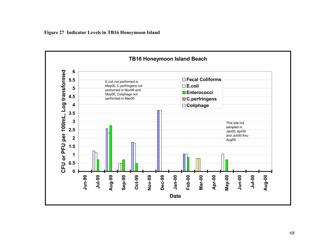
68

Figure 27 Indicator Levels in TB16 Honeymoon Island

TB16 Honeymoon Island Beach

0

0.5

1

1.5

2

2.5

3

3.5

4

4.5

5

5.5

6

Jun-

99

Jul-9

9

Aug

-99

Sep-

99

Oct

-99

Nov

-99

Dec

-99

Jan-

00

Feb-

00

Mar

-00

Apr

-00

May

-00

Jun-

00

Jul-0

0

Aug

-00

Date

CFU

or P

FU p

er 1

00m

L, L

og tr

ansf

orm

ed


This site not sampled in Jan00, Apr00 and Jun00 thru Aug00

E.coli not performed in May00, C.perfringens not performed in Nov99 and May00, Coliphage not performed in May00

69

Figure 28 Indicator Levels in TB22 Control Site

TB22 Control Site

0

0.5

1

1.5

2

2.5

3

3.5

4

4.5

5

5.5

6

Jun-

99

Jul-9

9

Aug

-99

Sep-

99

Oct

-99

Nov

-99

Dec

-99

Jan-

00

Feb-

00

Mar

-00

Apr

-00

May

-00

Jun-

00

Jul-0

0

Aug

-00

Date

CFU

or P

FU p

er 1

00m

L, L

og tr

ansf

orm

edFecal ColiformsE.coliEnterococciC.perfringensColiphage

This site not sampled Dec99, Jun00 thru Aug00

Fecal Coliforms and E.coli not performed in Mar00, Enterococci, Coliphage and C.per f r ingensnot performed in May 00.

70

Discussion of Indicator Data The highest individual sampling result for Fecal Coliforms occurred at TB4 Bullfrog Creek, with 174,900 cfu/100 mL. The highest arithmetic and geometric mean also occurred at site TB4, with 22,687 cfu/100 mL and 5032 cfu/100 mL, respectively. E.coli resulted in very similar numbers, again with site TB4 Bullfrog Creek. For Enterococci, the highest individual sampling result occurred at TB4, with 135,650 cfu/100 mL, and the high arithmetic mean of 14,520 cfu/100 mL and the geometric mean of 3009 cfu/100 mL occurring at TB4 as well. Clostridium perfringens had the highest individual sampling result of 160 cfu/100 mL at TB4, and the highest arithmetic mean of 32.7 cfu/100 mL occurring at TB4. The highest geometric mean, however, occurred at TB3 Bullfrog Creek, with a result of 11.3 cfu/100 mL. The highest individual sampling result for Coliphage occurred at TB4 with a result of 28,180 pfu/100 mL, and the highest arithmetic and geometric mean occurred at this site as well, with 2937 pfu/100 mL and 911 pfu/100 mL, respectively. For sites exceeding the suggested geometric guidelines, the two consistently high sites were TB4 Bullfrog Creek and TB14 Sweetwater Creek. The remaining sites along Bullfrog Creek (TB3, TB6, TB7 and TB8) were next among the highest sites when comparing indicator levels. Sites TB16 Honeymoon Island, TB19 John’s Pass and TB20 Ft. DeSoto were among the lowest sites when comparing geometric means of indicator levels. The months of Mar 00 and Dec 99 were the worst in terms of the most sites exceeding the Fecal Coliform guideline, with 15 and 13 sites respectively out of 22. Sep and Oct 99 follow closely behind with 10 sites out of 22 for both months. The months of Aug 99 and Jul 99 were the worst in terms of the most sites exceeding the Enterococci guideline, with 15 and 13 sites respectively out of 22. Sep, Oct and Nov 99 follow closely behind with 12, 11 and 10 sites out of 22 respectively. The months of Sep 99 and Oct 99 were the worst in terms of the most sites exceeding the Coliphage guideline, with 10 sites out of 22 for both months. Aug 99, Dec 99 and Jan 00 follow closely behind with 8 sites out of 22 for all three months. When looking at the seasonal graphs for each site, those located in rural areas show C. perfringens and coliphage occurring primarily in the winter and early spring months, whereas highly developed urban areas show these indicators occurring throughout the year. The exception to this is the Bullfrog Creek system, which shows indicator levels similar to that of urban sites. Most rural sites show a seasonal increase in indicator levels during the winter and early spring months, however, most urban sites are fairly consistent throughout the year. Fecal coliforms and E.coli levels were shown to peak without a corresponding peak in the other indicators.

71

E) Bacterial Source Tracking Background The goal of bacteriological water quality testing is to predict the risk of disease based on measured levels of bacteria and/or bacterial products. This goal has been elusive, in part because of the limitations of the methods we use. It is difficult, time-consuming and expensive to directly quantify disease-causing bacteria and viruses, and virtually impossible to test for all possible pathogens in a water sample. Thus, we quantify indicator bacteria, whose presence more-or-less reflects the probability that there are pathogens in the water. The problem with the fecal coliform indicator, in a nutshell, is that it is a poor predictor some human pathogens, particularly enteric viruses and protozoa, and may well be present in waters where there are few or no viral, bacterial or protozoan pathogens. One of the major reasons that fecal coliforms are inadequate indicators is that they are present in the gastrointestinal tract of all warm-blooded animals. Some animal feces, i.e. those of humans, cattle, and swine, have a higher probability of containing human pathogens than the feces of most other species, therefore these animals are included in the “high risk” group. Very low levels of fecal indicator bacteria from a high risk animal group would indicate a greater potential health hazard than higher levels of indicator bacteria from a low risk animal group. Currently, there is no routine testing method that can be used to determine the origin of fecal indicator bacteria, however, such a method would allow much more accurate risk assessment than we can achieve with standard testing methods. It would also allow regulatory agencies to more effectively identify and eliminate the source of bacterial contamination to natural waters. The enterococci (Enterococcus species) are another major group of indicator bacteria that have been adopted by the EPA and some other regulatory agencies as a bacteriological water quality indicator, particularly for marine and estuarine waters. Some studies have indicated that enterococcus levels are more closely correlated with cases of gastroenteritis in recreational waters than other indicator organisms (Cabelli et al., 1979; Cabelli,1983). The enterococci also survive longer under some environmental conditions, i.e. in saline waters, than fecal coliforms. However, the enterococci share the major disadvantage of the fecal coliform group; they are shed in the feces of all warm-blooded animals and therefore provide no indication of the source of fecal contamination. Bacterial Source Tracking. Bacterial Source Tracking (BST) is a term that refers to a group of methods that are used to type, or fingerprint, indicator bacteria such as fecal coliforms in order to determine their source, i.e. from human, dog, wild animal, etc. BST techniques that are currently in use measure characteristics such as antibiotic resistance to generate the fingerprint streams (Hagedorn et al., 1999; Harwood et al., 2000; Wagner and Harwood, 1999; Wiggins, 1996; Wiggins et al., 1999), or they may analyze differences at the level of the DNA fingerprint, as in ribotyping (Parveen et al.,1999. All

72

BST techniques rely on the establishment of a large database of “fingerprints” of indicator bacteria from known sources, i.e. humans, cattle, wild animals, etc. Fingerprints of bacteria isolated from water samples can then be statistically compared to the fingerprints in the database, allowing the investigator to determine the source of fecal contamination to the water. Bacterial resistance to antibiotics can be used to differentiate between indicator bacteria that are shed in the feces of various animals. Humans are exposed to a different set of antibiotics than are cattle, and poultry to a different set, and so on, while wild animals have relatively little exposure to antibiotics. Bacteria rapidly develop resistance to specific antibiotics when the animals in which they live are frequently treated with those antibiotics. It has been shown that antibiotic resistance patterns are significantly different in fecal indicator bacteria from different host sources, and that these differences are consistent enough that they can be used to predict the source of bacteria isolated from rivers and streams (Hagedorn et al., 1999; Harwood et al., 2000; Wagner and Harwood, 1999; Wiggins, 1996; Wiggins et al., 1999). The method, termed antibiotic resistance analysis (ARA) is carried out by first developing a database of antibiotic resistance patterns (ARPs) of indicator bacteria from known animal sources. Other investigators currently using this technique (Hagedorn and Wiggins) use fecal streptococci or enterococci as the indicator organism. Our laboratory uses both enterococci and fecal coliforms. In order to construct a database, fecal coliforms (for example) are isolated by membrane filtration from feces obtained from known animal sources. These isolates are plated on a battery of antibiotic-containing media and are scored positive or negative for growth on each plate. Currently we are using eight different antibiotics at four concentrations each, so the ARP of each isolate consists of 32 data points. The procedure for determining the ARPs of isolates requires four to five days. ARPs of bacteria from known sources are entered in a spread sheet. Discriminant analysis, a form of multiple analysis of variance, is used to analyze the data. Discriminant analysis uses the ARPs from known sources to generate the predictive equations (the “classification rule”) that will be used to classify unknown isolates by source. The accuracy of the database is assessed by using ARPs of the isolates from known sources as test data. This procedure generates a source-by-source matrix that provides the rate of correct classification for each source. Below is an example. The top number is number of isolates, the bottom is percent classified in a given category.

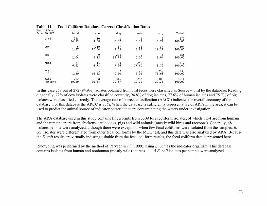
73

Table 11 Fecal Coliform Database Correct Classification Rates Fecal Coliforms From SOURCE bird cow dog huma pig Total bird 258 10 1 1 2 272 94.85 3.68 0.37 0.37 0.74 100.00 cow 6 219 17 25 37 304 1.97 72.04 5.59 8.22 12.17 100.00 dog 3 9 273 0 3 288 1.04 3.13 94.79 0.00 1.04 100.00 huma 21 15 23 246 12 317 6.62 4.73 7.26 77.60 3.79 100.00 pig 4 55 2 20 252 333 1.20 16.52 0.60 6.01 75.68 100.00 Total 292 308 316 292 306 1514 Percent 19.29 20.34 20.87 19.29 20.21 100.00 In this case 258 out of 272 (94.9%) isolates obtained from bird feces were classified as Source = bird by the database. Reading diagonally, 72% of cow isolates were classified correctly, 94.8% of dog isolates, 77.6% of human isolates and 75.7% of pig isolates were classified correctly. The average rate of correct classification (ARCC) indicates the overall accuracy of the database. For this database the ARCC is 83%. When the database is sufficiently representative of ARPs in the area, it can be used to predict the animal source of indicator bacteria that are contaminating the waters under investigation. The ARA database used in this study contains fingerprints from 3309 fecal coliform isolates, of which 1154 are from humans and the remainder are from chickens, cattle, dogs, pigs and wild animals (mostly wild birds and raccoons). Generally, 48 isolates per site were analyzed, although there were exceptions when few fecal coliforms were isolated from the samples. E. coli isolates were differentiated from other fecal coliforms by the MUG test, and this data was also analyzed by ARA. Because the E. coli results are virtually indistinguishable from the fecal coliform results, the fecal coliform data is presented here. Ribotyping was performed by the method of Parveen et al. (1999), using E. coli as the indicator organism. This database contains isolates from human and nonhuman (mostly wild) sources. 1 – 5 E. coli isolates per sample were analyzed

74

Enteroviruses are viruses that are thought to exclusively colonize humans, thus, they are specific indicators of human contamination. In this study, entervirus counts carried out on human cells lines were conducted to indicate the prevalence of human contamination at the Healthy Beaches sites. Five sites in each area (the Bullfrog Creek watershed and Pinellas County) were chosen for the BST analysis. The Bullfrog Creek sites were chosen to represent a course from the headwaters to the mouth of the creek, while the Pinellas County sites were chosen to represent freshwater (TB 14 and TB17, Gulf of Mexico (TB 19 and TB 20) and Tampa Bay (TB13) environments. Each site was sampled six times over the course of the study. Identification of Pollution from Human Sources. All sites displayed some level of human fecal pollution according to the three methods used (ribotyping, ARA and enterovirus counts). The three different methods did not always coincide on their prediction of the presence or absence of human contamination (see below), however the data collected over the course of the study unambiguously documents the presence of human fecal sources. A value called the Impact of Human Pollution (IHP) was devised in order to represent the combined results of the three methods of human source identification for each site. The percentage of human-positive sampling events for each site was first calculated for each site for each of the three methods. These values were added, then multiplied by 0.5 (for ease of graphical representation). For example, TB3 was human-positive by ribotyping in 33.3% of samples, by ARA in 80% of samples, and by enterovirus counts in 66.7% of samples. The IHP is calculated as (0.333 + 0.80 + 0.667)/2 = 0.90. Overall, sites in Bullfrog Creek (Figure 29) were more frequently impacted by human sources than sites in Pinellas County (Figure 30). Sites TB3 and TB4 in the Bullfrog Creek watershed were the sites most consistently impacted by human pollution. Bullfrog Creek is bordered by fairly intensive residential and commercial land use at TB3, and all wastewater treatment is by onsite wastewater treatment and disposal systems (OSTDS). TB4 is the closest downstream site to a septage spreading site that is now closed, but which was operational during the course of the study. While TB3 is the site closest to the mouth of Bullfrog Creek, TB8 is the site located at the headwaters, and Figure 1 reveals a steady decrease in human impact from urbanized TB3 to the rural TB8. A possible source of sporadic human contamination at TB8 is a residence with an OSTDS. The site most impacted in Pinellas County was Allan’s Creek (TB 17), followed closely by Sweetwater Creek (TB14) and the Courtney Campbell Causeway (TB13). The Gulf of Mexico beach sites included John’s Pass (TB19) and Fort DeSoto (TB20), which showed lower levels of human contamination than the freshwater and brackish water sites.

75

The Index of Human Pollution was significantly correlated with both Enterococcus (Figure 31) and fecal coliform (Figure 32) counts. For these analyses indicator organism counts are expressed as the geomean for each each site over the course of the study. Linear regression analysis yielded values of P < 0.05, r2 = 0.5023 for IHP vs. Enterococcus counts, and P < 0.05, r2 = 0.4832 for IHP vs. fecal coliforms counts. Of the individual source-specific techniques, only the percent enterovirus – positive sites was correlated with the average Enterococcus count for each site (P < 0.05, r2 = 0.4292). Two of the three source-specific methods correlated with average fecal coliform numbers; enterovirus (P < 0.05, r2 = 0.4728) and ribotyping (P < 0.05, r2 = 0.4265) were significantly correlated, while ARA was not. Agreement Between Source Tracking Methods. Agreement between the two bacterial source tracking methods (antibiotic resistance analysis and ribotyping) and enterovirus counts was assessed for each sampling event (Figure 33). Sites were scored positive for human impact when >20% of isolates were identified as human by ribotyping and by ARA, and when any enterovirus counts were detected. Sites were scored negative for human impact when <20% of isolates were identified as human by ribotyping and by ARA, and when no enterovirus counts were detected (<1/100 ml). Ribotyping and ARA results agreed for 31 of 53 samples (58.5%). Ribotyping and enterovirus results agreed for 29 of 52 (55.8%) samples. ARA and enterovirus results agreed most frequently, as positive results at the same sites were noted for 38 of 55 sampling events (69.1%). All three methods agreed for 21 of 51 samples (41.2%). There was no correlation between the percent of isolates identified as human by ribotyping and enterovirus counts. The Spearman rank correlation test (used for non-normally distributed data) showed a significant correlation between the percent of isolates identified as human by ARA and enterovirus counts (p < 0.05; r = 0.324). Fisher’s exact test for difference in frequency showed no significant difference in the percent of sites where methods agreed when comparisons were made between ARA vs. ribotyping, ARA vs. enterovirus, and ribotyping vs. enterovirus. Other Sources of Fecal Coliforms. Wild animals were the dominant source of fecal coliforms identified by antibiotic resistance analysis at each site (Figure 34). At TB 3, TB4 and TB6, human sources were almost equal those of wild animals. Recall that the Index of Human Pollution is also high at each of these sites. More isolates were assigned to the chicken and cattle categories in the Bullfrog Creek watershed (TB3 – TB8) than in the Pinellas County sites, which can be attributed to the agricultural activity that dominates the upper reaches of the watershed. In fact, chicken and cattle are insignificant sources (<10%) of isolates except at TB19, where 24.6% of all isolates were identified as from cattle. At only one sample event on 6/20/00 were cow isolates identified at TB19, when 48 of 48 fecal coliforms were typed as cattle isolates. One can speculate that this event may have been due to a hamburger wrapper from picnickers entering the water or some other unusual event. When a sporadic spike of contamination from a particular source occurs it is of less conern overall to watershed management than persistent input from a particular source. At the Pinellas County sites (13 – 20), wild animal sources were

76

particularly dominant (Figure 34). A prominent dog signal is present at TB20 (Fort DeSoto), which may be due to the practice of exercising dogs on the beach.

Discussion This study has shown that an approach that combines several source identification techniques can be useful for watershed assessment and management. Perhaps one of the most striking findings of this study is the extent to which wild animals dominate as a source of fecal coliform and E. coli isolates. Over the course of the study, wild animal isolates dominated each site according to ARA. The ribotyping analysis agreed; in 73.6% of all samples (n=53) the majority of isolates were identified as nonhuman. Nevertheless, all of the source-specific methods used in this study indicate that human pollution is significantly impacting the Bullfrog Creek watershed. This study suggests that OSTDS and associated activities may be a significant source of pollution to the Bullfrog Creek watershed, as there is no central sewer infrastructure in the watershed and there was at least one operational septage spreading site between TB4 and TB6. The consistent impact from human sources is less clear at the Pinellas County sites, although there are days when “spikes” of human isolates dominate these sites. For example, on 6/20/00 TB 17 (Allan’s Creek) 94% of fecal coliforms were identified as human isolates by ARA, 80% of isolates were human by ribotyping, and enterovirus were detected. However, such events are atypical of the Pinellas Creek sites, and were more likely to be observed at the Bullfrog Creek sites. The advantage to using a “toolbox” approach, where several source tracking methods are combined, is clear from this study. Identification of enterovirus in water represents a rigorous test for human contamination, however this technique is very expensive, and a negative result does not preclude human contamination. Two major advantages to ARA as performed in this study include (1) the fact that 48 – 96 isolates per sample can be readily analyzed, thus providing the investigator some assurance that the population is adequately sampled, and (2) non-human sources of contamination can also be identified. Ribotyping can also be used to identify non-human sources if the database is constructed adequately for that purpose; both Dr. Lukasik and Dr. Harwood are working on ribotyping databases to identify multiple sources. The percentage of isolates identified as human by ARA was significantly correlated with enterovirus counts, but the percentage of isolates identified as human by ribotyping was not significantly correlated with enterovirus counts. This discrepancy points to the need for including the fingerprints of more isolates from known, local sources in the respective databases. In the case of ARA, we have seen dramatic improvements in correct classification rates by adding fingerprints from local sources. The genetic and phenotypic variability of indicator bacteria such as E. coli is quite great, therefore any information that can be obtained on the fingerprints of actual contamination sources to a watershed is

77

extremely valuable. Encouragingly, ribotyping, ARA and enterovirus counts agreed on the presence/absence of human sources in 41.2% of samples. The probability of the three methods agreeing by chance alone is 0.125 (0.5 X 0.5 X 0.5), therefore the three methods agree on the presence of contamination far more frequently than would be predicted by a purely stochastic process.

Future Directions Databases (ribotyping and ARA) are currently under construction that will be more accurate than those used in this study. Although the current databases are valuable tools for environmental analysis, correct classification rates for isolates from known sources can be improved. We are also very interested in analysis of E. coli from sediments, as it has been shown that long survival times can be attained by fecal coliforms deposited to sediments. During times when sediment bacteria are resuspended by waves, current action, or human/animal activities, these organisms may comprise a significant portion of the population in surface water. We are also investigating the growth and survival of fecal coliforms, E. coli and Enterococcus species in the subtropical waters, soils and sediments of Florida.

78

Figure 29

Bacterial Source Tracking: Comparison of ARA, RT and Enterovirus in Bullfrog Creek Sites

0

10

20

30

40

50

60

70

80

90

100

Site3 Site 4 Site6 Site7 Site8

Perc

ent o

f Hum

an-P

ositi

ve S

ampl

es

ARARibotypeEnterovirusIndex

79

Figure 30

Bacterial Source Tracking: Comparison of ARA, RT and Enterovirus in Pinellas County Sites

0

10

20

30

40

50

60

70

80

Site13 Site 14 Site17 Site19 Site20

Perc

ent o

f Hum

an-P

ositi

ve S

ampl

es

ARARibotypeEnterovirusIndex

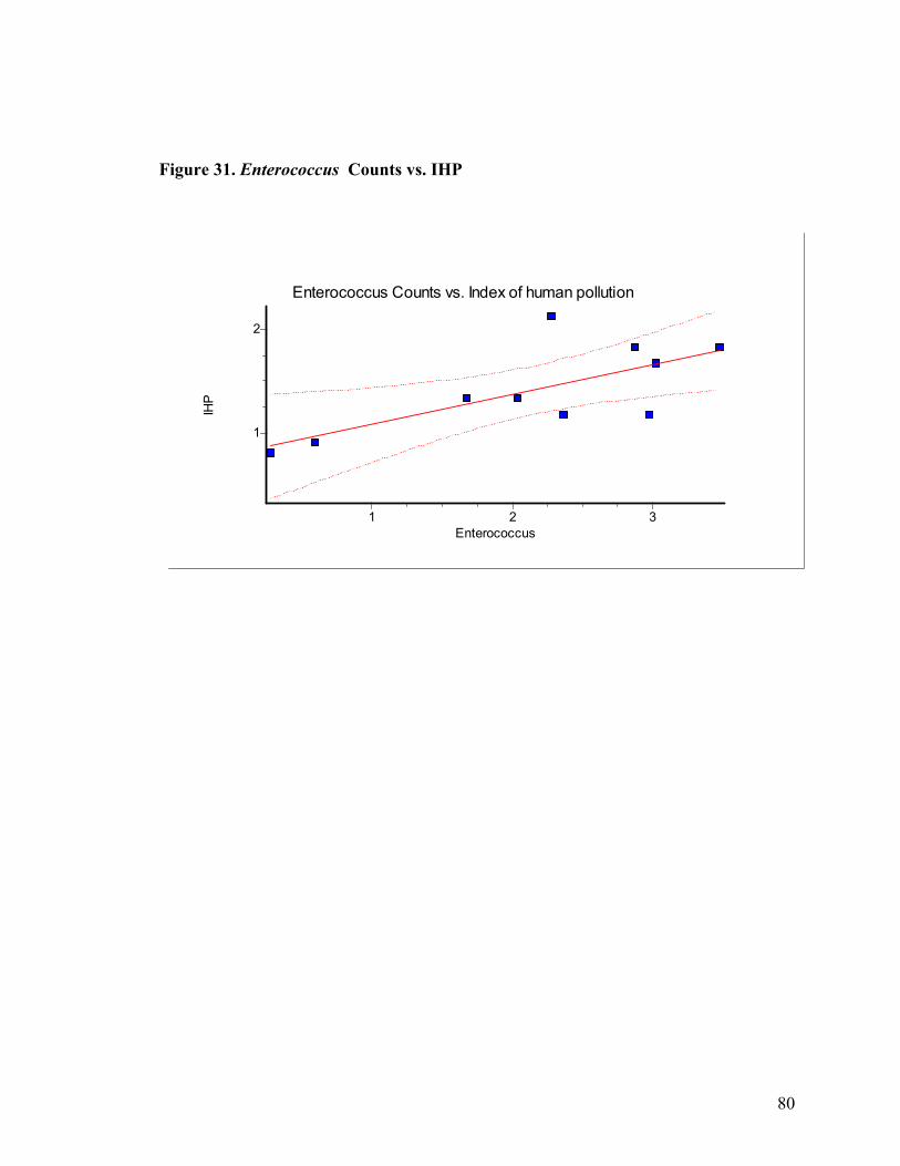
80

Figure 31. Enterococcus Counts vs. IHP

Enterococcus Counts vs. Index of human pollution

Enterococcus321

IHP

2

1

81

Figure 32. Fecal Coliform Counts vs. IHP

FC Counts vs. Index of human pollution

FC32

IHP

2

1

82

Figure 33

Agreement on Contamination by Human Sources Between RT, ARA and Enterovirus Counts

0.000

0.100

0.200

0.300

0.400

0.500

0.600

0.700

0.800

ARAvs.RT ARA(EC)vsRT ARAvs.Ent ARA(EC)vsEnt RT vs. Ent All three(FC) All three(EC)

Perc

ent A

gree

men

t

ARAvs.RTARA(EC)vsRTARAvs.EntARA(EC)vsEntRT vs. EntAll three(FC)All three(EC)

83

Figure 34

Note: Raw data of Ribotyping Results are found in Appendix VII

Sources of Fecal Coliforms at Healthy Beaches Sites

0

10

20

30

40

50

60

70

80

90

TB3 TB4 TB6 TB7 TB8 TB13 TB14 TB17 TB19 TB20

Perc

enta

ge o

f Iso

late

s A

ssig

ned

to S

ourc

e

% chick% cow% dog%human% pig% wild

84

F) Pathogen Monitoring Tables 12 and 13 below show the results of the Enterovirus monitoring for the 10 in-depth sampling sites (TB3, TB4, TB6-TB8 along Bullfrog Creek, TB14 Sweetwater Creek, TB17 Allen’s Creek, TB13 Courtney Campbell Causeway, TB19 John’s Pass and TB20 North Beach, Ft. DeSoto). The site designation, month of sampling, and results in MPN-PFU per 100 L of water are given in Table 12. Of the 59 samples collected for virus testing, twenty-three (47%) were positive. The raw data reports for the Enterovirus analysis can be found in Appendix VIII. One or two positive results were detected each month, however, the highest number of isolations were found in September and October 1999 (with 3 and 4 sites positive out of 5, respectively), which corresponds to the indicator peak found in the rural sites during October 1999, and the September 1999 peak found in the urban and beach sites. The virus levels ranged from 1.1 to 27.1 MPN-PFU/100 L Table 13 summarizes the positive results for each of the sampling sites. Bullfrog Creek overall shows consistent Enterovirus results, with TB3 and TB4 showing the highest percentage of positive results. The two urban sites, and the three beach sites had 1-2 positive results during the length of the study. A Table showing the parasite data can be found in Appendix IX. Out of 20 samples collected from the in-depth sites (10 sites sampled 2 times during the study), no Giardia were detected during the study. Sites TB3, TB4, TB7 and TB8 along Bullfrog Creek all showed the presence of Cryptosporidium with results of 3.48 oocysts per 100 L of water for TB7, 7.03 oocysts/100 L for TB8, 124.4 oocysts/100 L for TB4 and 470 oocysts/100 L for TB3. Each site tested positive for Cryptosporidium only once during the study. Table 12 Enterovirus Levels in Tampa Bay Site Date Enterovirus MPN/100 L

TB3 Aug 99 2.3 TB4 Aug 99 7.0 TB6 Aug 99 Neg <0.95 TB7 Aug 99 Neg <1.1 TB8 Aug 99 Neg <1.2 TB13 Sept 99 Neg <1.1 TB14 Sept 99 Neg <1.2 TB17 Sept 99 8.4 TB19 Sept 99 1.1 TB20 Sept 99 2.7 TB3 Oct 99 5.1 TB4 Oct 99 7.1 TB6 Oct 99 2.4

85

Table 12 con’t Site Date Enterovirus MPN/100 L TB7 Oct 99 9.4

TB8 Oct 99 Neg <0.95 TB4 Dec 99 27.1 TB6 Dec 99 Neg <1.02 TB7 Dec 99 Neg <1.01 TB8 Dec 99 11.3 TB13 Feb 00 Neg <1.05 TB14 Feb 00 Neg <1.08 TB17 Feb 00 Neg <1.12 TB19 Feb 00 Neg <0.75 TB20 Feb 00 Neg TB3 Mar 00 1.26 TB4 Mar 00 Neg <1.03 TB6 Mar 00 Neg <1.10 TB7 Mar 00 1.23 TB8 Mar 00 Neg <1.00 TB13 Apr 00 1.2 TB14 Apr 00 Neg <1.1 TB17 Apr 00 Neg <1.1 TB19 Apr 00 Neg <1.1 TB20 Apr 00 Neg <1.1 TB13 May 00 1.2 TB14 May 00 Neg <1.0 TB17 May 00 Neg <1.1 TB19 May 00 Neg <1.1 TB13 Jun 00 Neg <1.2 TB14 Jun 00 10.9 TB17 Jun 00 1.2 TB19 Jun 00 Neg <1.1 TB20 Jun 00 Neg <1.1 TB3 July 00 Neg <1.2 TB4 July 00 1.3 TB6 July 00 2.5 TB7 July 00 Neg <1.1 TB8 July 00 Neg <1.1 TB3 Aug 00 1.1 TB4 Aug 00 Neg <1.2 TB6 Aug 00 4.3 TB7 Aug 00 Neg <1.1 TB8 Aug 00 1.1 TB13 Aug 00 Neg <1.1 TB14 Aug 00 4.3

86

Table 12 con’t Site Date Enterovirus MPN/100 L TB17 Aug 00 Neg <1.1 TB19 Aug 00 Neg <1.2 TB20 Aug 00 Neg <1.2 Table 13 Percentage of Enterovirus Positives by Site Site Type Site # of samples positive Total samples collected Rural TB3 Bullfrog 4 5 TB4 Bullfrog 4 6 TB6 Bullfrog 3 6 TB7 Bullfrog 2 6 TB8 Bullfrog 2 6 Urban TB14 Sweetwater 2 6 TB17 Allen’s 2 6 Beach TB13 Courtney C. 2 6 TB19 John’s Pass 1 6 TB20 Ft. Desoto 1 6 G) Bacteroides fragilis Phage Assay The alternative indicator, Bacteroides fragilis phage, was investigated as a possible alternative viral indicator. The summary of this section of the study can be found in Appendix X. The phage was detected, but in very low concentrations, which makes the assay difficult to use. The human strain of the phage, B40-8 was detected in 6 of the 22 sampling sites, or 27% of the total sites. The phage was detected at TB4 and TB7 along Bullfrog Creek, TB1 Delaney Creek, TB12 Hillsborough River, TB14 Sweetwater Creek and TB17 Allen’s Creek, and never at any of the beach sites. The high level of the animal/human strain of the phage, B56-3, found in domestic sewage indicates a human source for this phage in the environment, but when it is detected in the environment, it is difficult to trace the source.

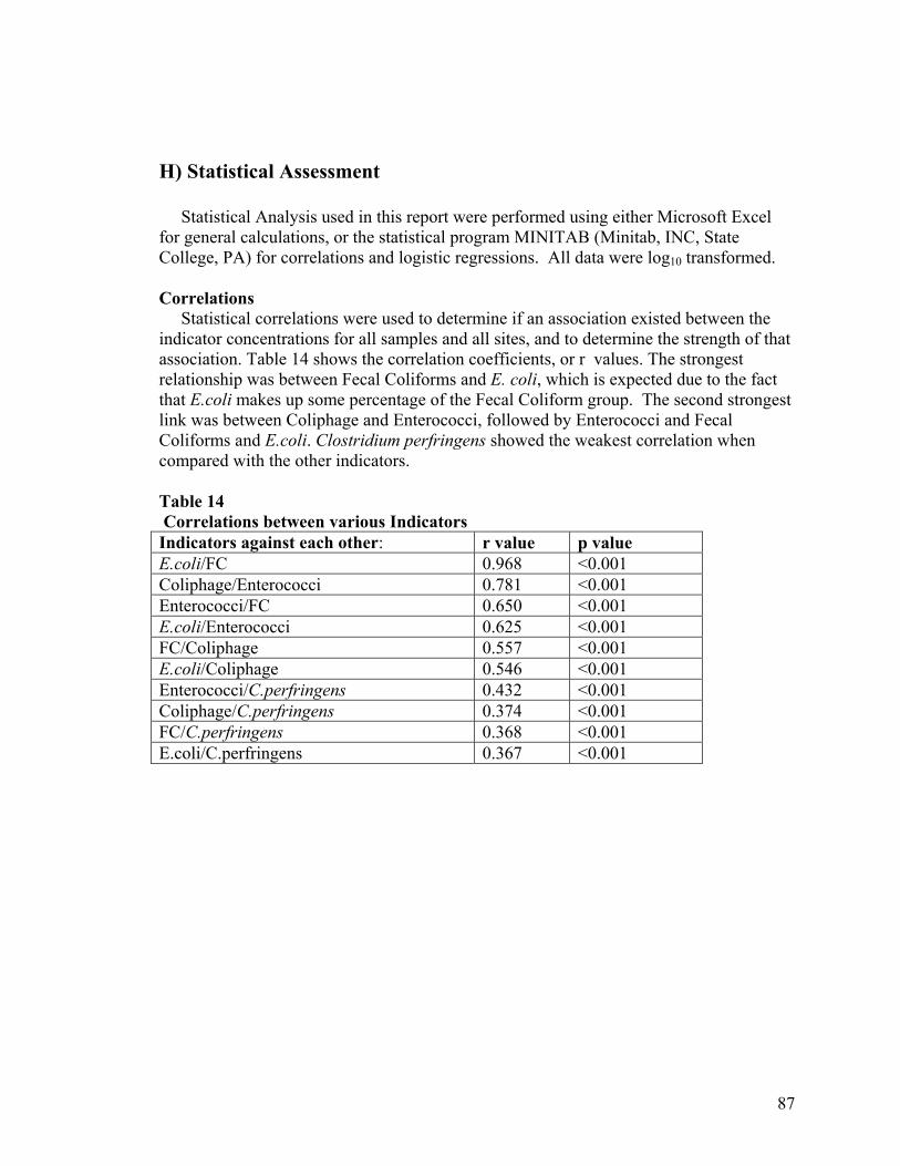
87

H) Statistical Assessment Statistical Analysis used in this report were performed using either Microsoft Excel for general calculations, or the statistical program MINITAB (Minitab, INC, State College, PA) for correlations and logistic regressions. All data were log10 transformed. Correlations Statistical correlations were used to determine if an association existed between the indicator concentrations for all samples and all sites, and to determine the strength of that association. Table 14 shows the correlation coefficients, or r values. The strongest relationship was between Fecal Coliforms and E. coli, which is expected due to the fact that E.coli makes up some percentage of the Fecal Coliform group. The second strongest link was between Coliphage and Enterococci, followed by Enterococci and Fecal Coliforms and E.coli. Clostridium perfringens showed the weakest correlation when compared with the other indicators. Table 14 Correlations between various Indicators Indicators against each other: r value p value E.coli/FC 0.968 <0.001 Coliphage/Enterococci 0.781 <0.001 Enterococci/FC 0.650 <0.001 E.coli/Enterococci 0.625 <0.001 FC/Coliphage 0.557 <0.001 E.coli/Coliphage 0.546 <0.001 Enterococci/C.perfringens 0.432 <0.001 Coliphage/C.perfringens 0.374 <0.001 FC/C.perfringens 0.368 <0.001 E.coli/C.perfringens 0.367 <0.001

88

The indicators were compared to the presence of Enteroviruses, and in Table 15, the strongest correlation existed between Enterovirus and Enterococci, followed by Coliphage, Fecal Coliforms and E.coli. Clostridium perfringens showed no correlation to the presence of Enteroviruses. The correlations are low, with the highest only at 0.553, but this is not uncommon for environmental samples. Table 15 Correlations between Viruses and Indicators Indicators against entervirus: r value p value Enterovirus/Enterococci 0.553 <0.001 Enterovirus/Coliphage 0.457 <0.001 Enterovirus/FC 0.442 0.001 Enterovirus/E.coli 0.370 0.010 Enterovirus/C.perfringens 0.199 0.137 Predicting the presence of Enterovirus with Indicator Results All samples that had enterovirus results were compared to the indicator results for each individual indicator, and for combinations of indicators. The samples below the indicator guidelines suggesting safe levels were then compared with those sites that tested positive for Enteroviruses. The results are shown in Table 16a-c. The individual indicators are shown in Table 16a and combinations of indicators are shown in Table 16b. Percentages using only the beach sites for comparison are shown in Table 16c. The first row in all 3 tables is the number of samples below the guidelines out of the total sample set. The next row is the number of those samples below the guideline that also had a positive virus result, and the last row shows those samples below the guidelines that had a negative virus result. When the indicators were above the recommended guidelines, the percentage of positive Enterovirus results were 53% for fecal coliforms, 51% for Enterococci, 59% for coliphage and 50% for Clostridium perfringens. When the indicators were below the suggested guidelines as shown in the table, the percentage of positive Enterovirus results were 16% for Fecal Coliforms, 19% for Enterococci, 22% for Coliphage and 30% for Clostridium perfringens. When the indicators were combined, the percentage of positive virus results occurring when the indicators were below the guidelines lessened. The most successful combination was Fecal Coliforms and Enterococci, with only 6% of the samples under the guidelines for both showing a positive virus result. When the beach sites were analyzed separately, the same combination of Fecal Coliforms and Enterococci gave the best percentage, with 8% of the samples under the guidelines for both indicators showing a positive virus result.

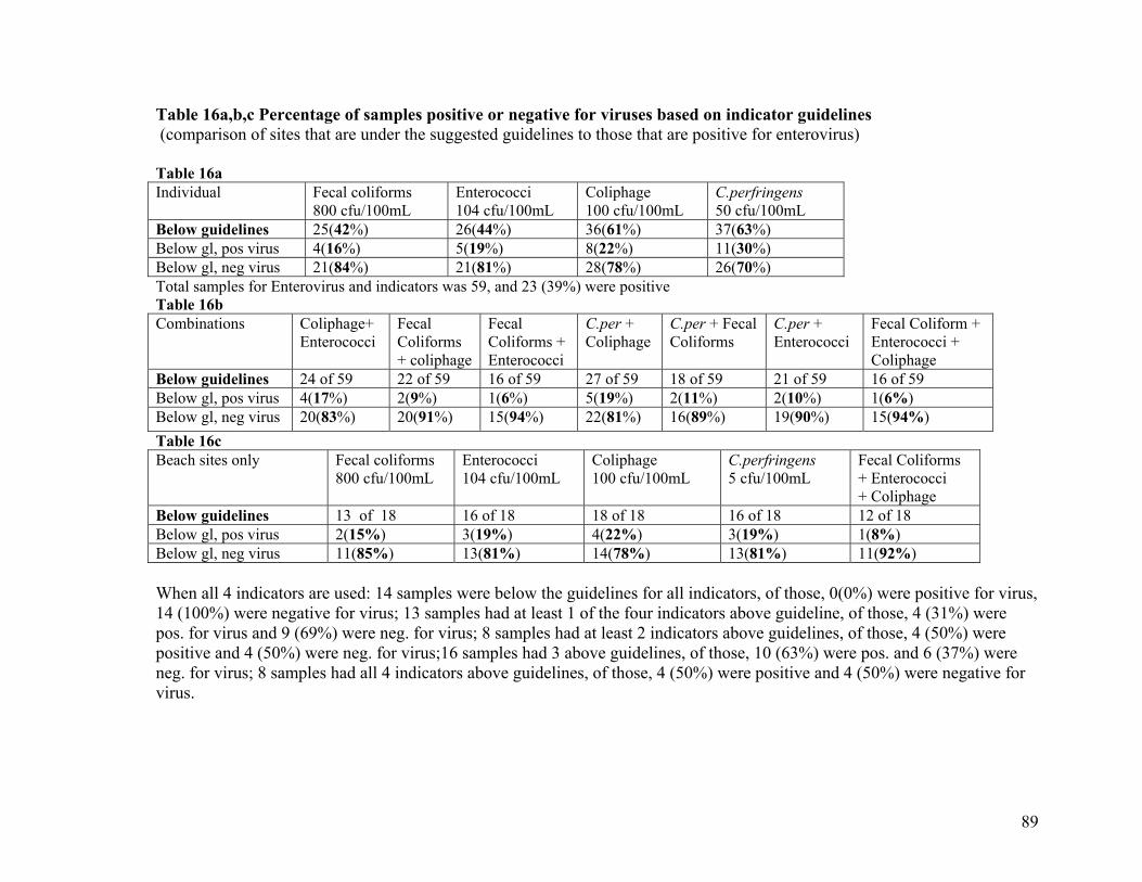
89

Table 16a,b,c Percentage of samples positive or negative for viruses based on indicator guidelines (comparison of sites that are under the suggested guidelines to those that are positive for enterovirus) Table 16a Individual Fecal coliforms

800 cfu/100mL Enterococci 104 cfu/100mL

Coliphage 100 cfu/100mL

C.perfringens 50 cfu/100mL

Below guidelines 25(42%) 26(44%) 36(61%) 37(63%) Below gl, pos virus 4(16%) 5(19%) 8(22%) 11(30%) Below gl, neg virus 21(84%) 21(81%) 28(78%) 26(70%) Total samples for Enterovirus and indicators was 59, and 23 (39%) were positive Table 16b Combinations Coliphage+

Enterococci Fecal Coliforms + coliphage

Fecal Coliforms + Enterococci

C.per + Coliphage

C.per + Fecal Coliforms

C.per + Enterococci

Fecal Coliform + Enterococci + Coliphage

Below guidelines 24 of 59 22 of 59 16 of 59 27 of 59 18 of 59 21 of 59 16 of 59 Below gl, pos virus 4(17%) 2(9%) 1(6%) 5(19%) 2(11%) 2(10%) 1(6%) Below gl, neg virus 20(83%) 20(91%) 15(94%) 22(81%) 16(89%) 19(90%) 15(94%) Table 16c Beach sites only Fecal coliforms

800 cfu/100mL Enterococci 104 cfu/100mL

Coliphage 100 cfu/100mL

C.perfringens 5 cfu/100mL

Fecal Coliforms + Enterococci + Coliphage

Below guidelines 13 of 18 16 of 18 18 of 18 16 of 18 12 of 18 Below gl, pos virus 2(15%) 3(19%) 4(22%) 3(19%) 1(8%) Below gl, neg virus 11(85%) 13(81%) 14(78%) 13(81%) 11(92%) When all 4 indicators are used: 14 samples were below the guidelines for all indicators, of those, 0(0%) were positive for virus, 14 (100%) were negative for virus; 13 samples had at least 1 of the four indicators above guideline, of those, 4 (31%) were pos. for virus and 9 (69%) were neg. for virus; 8 samples had at least 2 indicators above guidelines, of those, 4 (50%) were positive and 4 (50%) were neg. for virus;16 samples had 3 above guidelines, of those, 10 (63%) were pos. and 6 (37%) were neg. for virus; 8 samples had all 4 indicators above guidelines, of those, 4 (50%) were positive and 4 (50%) were negative for virus.

90

One way analysis of variance Analysis of Variance, or ANOVA’s , were used to determine if the sampling sites could be grouped into similar categories in regard to the indicator results. Although some variation exists, the results of the ANOVA’s agree with the observation from the geometric mean and seasonal graphs. The control site (TB22), Honeymoon Island (TB16), North Beach (TB20), and John’s Pass (TB19) tend to fall into one group, and Sweetwater Creek (TB14) and all sites along Bullfrog Creek (TB3, TB4, TB6, TB7 and TB8) tend to fall into another category. The other sites are scattered between these two groups. The ANOVA’s were run using the statistical software MINITAB (Minitab, Inc, PA) and GraphPad Prism (Intuitive Software for Science, CA). Both software packages gave similar results. The tables showing the individual ANOVAs and summary sections are given in the Appendix XI.

91

I) Climate Effects, Physical/Chemical Variables and Water Quality Rainfall and Stream flow for Tampa Bay Watersheds Microbial water quality was compared to climate factors (rainfall, stream flow and temperature) as well as chemical/physical variables (salinity, turbidity and pH). The rainfall and stream flow gage stations and databases used in this study are listed in Appendix XI along with the website locations of the different databases. The Southwest Florida Water Management District monthly hydrologic reports (found on SWFWMD website) were used for the monthly rainfall averages for the entire district (covering the entire sampling area around Tampa Bay) and are shown in Table 17. The highest rainfall during the sampling schedule occurred June through September 1999 and started to peak again in June and July 2000. The late winter and spring months showed relatively little rainfall. Totaling the individual rainfall and stream flow stations throughout the watersheds (See Appendix XII) resulted in a very similar pattern to the hydrologic data supplied by SWFWMD, with the highest and lowest months agreeing in each case. Table 17 Monthly Rainfall Averages for Tampa Bay Month Ave Monthly Rainfall in inches

June 1999 9.3 July 1999 5.75

August 1999 8.12 September 1999 6.13

October 1999 3.33 November 1999 1.97 December 1999 1.84 January 2000 1.59 February 2000 0.54 March 2000 1.01 April 2000 Not available May 2000 0.42 June 2000 7.20 July 2000 8.18

August 2000 Not available Table 18 shows the months that exhibited a peak in the traditional and alternative indicators for each individual sampling site. When the sites were divided as urban and rural, the rural sites mainly peaked in Oct 99 and Mar 00, while the urban sites were more varied, with peaks in Sept 99, Dec 99, Mar 00 and Feb 00. When looking at the monthly averages (Table 17) and comparing them to the indicator peaks (Table 18), the Oct 99 peaks occurred at the end of the rainy season (months of highest rainfall for the year).

92

The Mar 00 peak could not be linked to increased rain, occurring at a fairly dry time of the year. In addition, indicator peaks in Dec 99 were not linked with monthly increase in rain. Table 18 Traditional and Alternative Indicator Peaks Sampling site Months that exhibited indicator peaks TB1 Oct 99, Mar 00 TB2 Oct 99, Mar 00 TB3 Oct 99, Mar 00 TB4 Oct 99, Mar 00, Jul 00 TB5 Oct 99, Mar 00 TB6 Oct 99, Jan 00, Feb 00 TB7 Aug 99, Oct 99, Dec 99, Mar 00 TB8 Oct 99, Dec 99 TB9 Oct 99, Mar 00 TB10 Oct 99, Mar 00 TB11 Mar 00 TB12 Dec 99, Feb 00, Mar 00 TB13 Sept 99, Mar 00 TB14 Dec 99 TB15 Mar 00 TB16 Dec 99 TB17 Sept 99 TB18 Dec 99 TB19 Sept 99, Dec 99 TB20 Sept 99, Dec 99, Feb 00, Mar 00 TB21 Dec 99, Feb 00, Mar 00 TB22 None Correlations – Indicators and Rainfall/Stream flow Correlations between rainfall, stream flow and the traditional and alternative indicators for each individual site, as well as different groupings of sampling sites, were run using the statistical program MINITAB (Minitab,INC, State College, PA) Indicator levels were compared to rainfall using 3 day total and average values, 7 day total and average values, 10 day total and average values, and in some cases, 30 day average values. The rainfall and stream flow averages and totals used in the comparison were combined from all gage stations found within each watershed area for the rural sites. For Pinellas county, the gage stations were grouped into north and south Pinellas county, and then the sites were compared with a grouping depending on where the sampling site was located within the county. Correlations with indicator levels using rainfall and stream flow measurements from only the gage station closest to the sampling site did not correlate as well as when all gage stations in the watershed or in the surrounding areas were combined and then compared to the indicator levels.

93

When all the sampling sites were combined into one data set and compared with the indicator levels, no correlation between rainfall, stream flow and the indicator values was found. Using individual sampling sites and groupings of sites into rural, urban and beach sites, however, did result in the following correlations. Fecal Coliforms and E.coli did not show any correlation to rainfall and stream flow except in the Alafia watershed (sites TB2 and TB5) and Joe’s Creek/Cross Bayou system (TB18). In these cases, the r value for Fecal Coliforms compared to 7 day total stream flow was 0.429 (p=0.037) for the Alafia watershed (TB2 and TB5), and the r value for Fecal Coliforms compared to 3 day total rainfall was 0.721 (p=0.019) in Joe’s Creek (TB18). For E.coli, the r value when compared to 10 day total stream flow was 0.469 (p=0.043) for the Alafia watershed, and was 0.711 (p=0.032) when compared to 3 day total rainfall in Joe’s Creek. Greater associations were found with the other indicators and rainfall/stream flow data (Tables 19-21). In Table 19, the values are given for correlations with Enterococci within the individual watersheds. The sites are listed in the grouping of rural, urban and beach sites. Each result shows the r value, p value and whether the total or average rainfall or stream flow measurement for the length of days was used in the comparison. The highest correlations for this indicator occurred in the urban site group, with sites TB12, TB15 and TB17 showing individual correlations with 7 day rainfall, with r values of 0.942 (p=<0.001), 0.932 (p=<0.001) and 0.714 (p=0.006), respectively. Site TB12 showed a correlation with 7 day stream flow, with an r value of 0.856 (p=0.002). Several smaller correlation values occurred within the watersheds of the rural group for both rainfall and stream flow. No correlations were found within the beach sites. Table 20 shows the correlations for C.perfringens, in which associations with rainfall were found. For sites TB2 and TB5 (Alafia River), the r value was 0.586 (p=0.005) when the 3 day total rainfall was compared to Clostridium levels. The 3 day total rainfall for site TB17 Allen’s Creek resulted in a correlation with an r value of 0.646 (p=0.023), and the 10 day total and average rainfall for site TB18 Joe’s Creek resulted in a correlation with an r value of 0.769 (p=0.026) when compared to the level of Clostridium. An inverse correlation resulted for site TB11 Manatee River and for the beach site TB19 John’s Pass, with r values of –0.677 (p=0.032) and –0.615 (p=0.033), respectively. Coliphage (Table 21) were correlated with rainfall and stream flow in the watersheds within the rural grouping. The one and highest correlation at the urban site TB12 Hillsborough River had an r value of 0.895 (p=0.001) associating coliphage with rainfall. All the sites within each of the 3 groupings (rural , urban and beach sites) were combined into a data set and the indicators were compared to the rainfall and stream flow measurements within these 3 groups. The results of the correlations are found in Table 22a-b. For the rural group, no correlations were found. In the urban data set, only rainfall correlated to Enterococci, C. perfringens and Coliphage levels, with r values of 0.350 (p=0.002), 0.334 (p=0.002) and –0.557 (p=0.009), respectively. The beach sites correlated with 10 day average rainfall with an r value of 0.310 (p=0.030) for Enterococci and an r value of –0.304 (p=0.036) when 7 day total rainfall was compared with Coliphage results.

95

Table 19 Correlations between Enterococci Levels and Rainfall/Stream flow Site Rainfall (r value, p value, total or ave used) Stream flow (r value, p value, tot or ave used) 3 day 7 day 10 day 3 day 7 day 10 day Rural TB1 0.597 Total

(p=0.041)

TB2 & 5 0.516 Tot/Avg (p=0.014)

0.546 Tot/Avg (p=0.009)

TB3/8 0.275 Total (p=0.027)

0.484 Tot/Avg (p=<0.001)

TB9 & 10 0.469 Tot/Avg (p=0.021)

TB11 Urban TB12 0.942 Tot/Avg

(p=<0.001) 0.856 Tot/Avg

(p=0.002)

TB14 0.560 Average (p=0.047)

TB15 0.932 Total (p=<0.001)

TB17 0.714 Total (p=0.006)

TB18 TB21 Beach TB13 TB16 TB19 TB20

96

Table 20 Correlations between Clostridium perfringens Levels and Rainfall/Stream flow Site Rainfall (r value, p value and total or average used) Stream flow (r value, p value, tot/av) 3 day 7 day 10 day 3 day 7 day 10 day Rural TB1 TB2 & 5 0.586(p=0.005)

Total

TB3/8 TB9 & 10 TB11 -0.677 (p=0.032)

Average

Urban TB12 TB14 0.632(p=0.030)

Tot/Avg

TB15 TB17 0.646(p=0.023)

Total

TB18 0.769 (p=0.026) Tot/Avg

TB21 Beach TB13 TB16 TB19 -0.615 (p=0.033)

Average

TB20

97

Table 21 Correlations between Coliphage Levels and Rainfall/Stream flow Site Rainfall (r value, p value, tot or ave used) Stream flow ( r value, p value, tot or ave used) 3 day 7 day 10 day 3 day 7 day 10 day Rural TB1 0.639(p=0.034)

Total

TB2 & 5 0.535(p=0.010) Tot/Avg

TB3/8 0.280(p=0.024) Tot/Avg

TB9 & 10 0.503(p=0.017) Total

TB11 0.723(p=0.018) Tot/Avg

Urban TB12 0.895(p=0.001) Average

TB14 TB15 TB17 TB18 TB21 Beach TB13 TB16 TB19 TB20

98

Tables 22a,b Correlations between Site groups and Rainfall/Stream flow Table 22a Urban Sites Rainfall (r value, p value and total or average values used) Stream flow 3 day 7 day 10 day 3 day 7 day 10 day Fecal Coliforms

E.coli Enterococci 0.350 (p=0.002) Total C. perfringens 0.334 (p=0.005) Total Coliphage -0. 557 (p=0.009) Tot/Avg Table 22b Beach Sites Rainfall (r value, p value and total or average value used) Stream flow 3 day 7 day 10 day 3 day 7 day 10 day Fecal Coliforms

E.coli Enterococci 0.310 (p=0.030) Avg C. perfringens Coliphage -0.304(p=0.036) Total

99

Effects of Salinity, Turbidity, Temperature and pH The correlations comparing the five indicator levels to salinity, turbidity, temperature and pH are given in Table 23a-d. The sites were combined into rural, urban, and beach sites again, as well as a group with just the Bullfrog Creek sites. For the rural sites, salinity gave inverse correlations for all indicators except C. perfringens, with r values ranging from –0.241 (p=0.011) for E.coli to –0.422 (p=<0.001) for Enterococci. The pH correlations showed similar results to salinity. Turbidity correlated only with Fecal Coliforms , with an r value of 0.363 (p=<0.001). Temperature also correlated with all indicators except Fecal Coliforms, with r values ranging from 0.239 (p=0.011) for C. perfringens to 0.442 (p=<0.001) for Enterococci. The urban sites showed inverse correlations with salinity for Enterococci, C.perfringens and Coliphage, with r values of –0.229 (p=0.048), -0.285 (p=0.010) and -0.306 (p=0.011), respectively. No correlations were found with turbidity, and temperature only resulted in a correlation with C. perfringens, with an r value of 0.311 (p=0.010). Fecal Coliforms and E.coli correlated inversely with pH, with r values of –0.388 (p=<0.001) and –0.412 (p=<0.001), respectively. For the beach sites, salinity inversely correlated with Fecal Coliforms, Enterococci and C.perfringens, with r values of –0.341 (p=0.018), -0.616 (p=<0.001) and –0.500 (p=0.001), respectively. Turbidity correlated with Enterococci, with an r value of 0.290 (p=0.046), and no correlations were found with temperature and pH. When Bullfrog Creek was studied as a group, salinity, temperature and pH showed little, if any, correlation with the indicator levels. Turbidity, however, showed an r value of 0.453 (p=<0.001) for Fecal Coliforms, similar results for E.coli, , 0.556 (p=<0.001) for Enterococci, and 0.642 (p=<0.001) for Coliphage. The Bullfrog Creek system is very shallow in most parts, and this could explain the strong relationship between turbidity and the indicator values for this creek. (This system is also a primarily freshwater system, which may contribute to this relationship as well) Table 22 shows the correlations for all sites combined into one data set. Overall, salinity results in an inverse correlation with all indicators, ranging from –0.288 (p=<0.001) for C.perfringens to –0.650 (p=<0.001) for Enterococci. The correlations for pH showed a similar result to salinity, and there was no correlation with the indicators and turbidity. Temperature showed weaker inverse correlations with the indicators, ranging from –0.137 (p=0.035) for Enterococci to –0.232 (p=<0.001) for Coliphage. No correlation was found between C.perfringens and temperature.

101

Tables 23 a-d Correlations between Indicator Levels and Physical/Chemical Variables for site groupings Rural Sites Salinity (r/p values) Turbidity Temperature pH Fecal Coliforms -0.278 (p=0.001) 0.364 (p=<0.001) -0.290 (p=0.001) E.coli -0.241 (p=0.011) 0.384 (p=<0.001) -0.327 (p=0.001) Enterococci -0.422 (p=<0.001) 0.442 (p=<0.001) -0.361 (p=<0.001) C.perfringens 0.239 (p=0.011) Coliphage -0.354 (p=<0.001) 0.432 (p=<0.001) -0.428 (p=<0.001) Urban Sites Salinity (r/p values) Turbidity Temperature pH Fecal Coliforms -0.388 (p=<0.001) E.coli -0.412 (p=<0.001) Enterococci -0.285 (p=0.010) C.perfringens -0.306 (p=0.011) 0.311 (p=0.010) Coliphage -0.229 (p=0.048) Beach Sites Salinity (r/p values) Turbidity Temperature pH Fecal Coliforms -0.341 (p=0.018) E.coli Enterococci -0.616 (p=<0.001) 0.290 (p=0.046) C.perfringens -0.500 (p=0.001) Coliphage Bullfrog Creek Salinity (r/p values) Turbidity Temperature pH Fecal Coliforms 0.453 (p=<0.001) E.coli 0.458 (p=0.001) Enterococci -0.355 (p=0.004) 0.556 (p=<0.001) C.perfringens 0.290 (p=0.023) Coliphage 0.642 (p=<0.001) 0.275 (p=0.033)

102

Table 24 Correlations between Indicator Levels and Physical/Chemical Variables for entire data set All Sites Salinity (r/p values) Turbidity Temperature pH Fecal Coliforms -0.389 (p=<0.001) -0.181 (p=0.005) -0.357 (p=<0.001) E.coli -0.386 (p=,0.001) -0.142 (p=0.042) -0.392 (p=<0.001) Enterococci -0.650 (p=<0.001) -0.137 (p=0.035 -0.468 (p=<0.001) C.perfringens -0.288 (p=<0.001) -0.212 (p=0.002) Coliphage -0.649 (p=<0.001) -0.232 (p=<0.001) -0.402 (p=<0.001)

Viruses and Climatic/Environmental Association Binary Logistic Regressions were used to determine the relationship between rainfall, stream flow and the presence of Enterovirus. A slightly significant logistic regression result occurred within the beach site grouping between the 7 day average rainfall values and the presence of Enterovirus, resulting in a 64.3% concordant percentage, 30.4% discordant percentage and a 5.4% tie. Salinity and Enterovirus in this same beach grouping resulted in a concordant percentage of 69.6%, 26.8% discordant percentage and a 3.6% tie. No other significant relationship was found between the climate factors used in the study, and the presence or absence of Enterovirus. The virus data set for this study is small, however, and a more intensive virus sampling regime may be needed for a more accurate statistical analysis of climate factors and their contribution to virus water quality. Summary of Climate and Indicators The Fall peak in fecal indicator levels corresponds to the end of the rainy season, however, the Spring peak cannot be linked to rainfall or stream flow parameters. A lag time beyond 30 days exists when rainfall is compared to the indicators, but localized peaks associated with rainfall events may still occur within individual watersheds. Total rainfall rather than average rainfall was better than stream flow for correlations overall. For Enterococci, the 7 day total was useful, but for coliphage, the 3 day total was better perhaps because of the decreased survival in warm tropical waters. Average rainfall for beach sites was useful only when looking widely at the Bay, not for the individual sites. Enterococci compared to the 10 day rainfall was the only useful indicator at the beach sites. Negative correlations to rainfall and stream flow suggest that in some watersheds dilution due to increased rainfall and stream flow will actually decrease the number of phage and Clostridium. Both coliphage and Clostridium were found in low numbers compared to the other indicators. Sources are more likely to be related to feces compared to coliforms and Enterococci, which might have a soil or vegetative source. And while Clostridium could accumulate in sediments and does survive for extended periods of time, the low concentrations make it susceptible to non-detects when fresh water increases.

104

IV. SUMMARY, CONCLUSIONS AND RECOMMENDATIONS

The need for new approaches to study microbial water quality

Water quality is influenced by a number of factors; these include land use patterns and population growth as well as climate factors. Historically, water quality in Tampa Bay has been impacted by these same factors. Nutrients have been the focus of many of the water quality studies, yet through efforts of the Tampa Bay Estuary Program and county and city agencies as well as the private sector a plan for the reduction of nutrients has been formulated. In fact, the addition of denitrification processes at the Howard Curren facility and other efforts have lead to a reduction of nitrogen and an increase in the coverage of sea grasses, which in turn will improve the overall ecosystem and fisheries potential.

While much attention has been paid to nutrients it is only in recent years that the

problem of microbiologically-contaminated waters has been highlighted. The sources of microorganisms include wastewater discharges, septic tanks, animal wastes, septage, and wildlife. The use of waters for recreational purposes (swimming, fishing, boating) as well as for drinking water supply (eg. Hillsborough river and desalination) that are contaminated can be linked to human illnesses. Total and fecal coliform bacteria (two related groups) have been used to study microbial water quality. However, these tests are inadequate. Total coliform bacteria should no longer be used in ambient water monitoring in Florida. While fecal coliform bacteria are suggested to more readily tied to fecal contamination and the sources mentioned above there are some significant problems associated with this test particularly for subtropical waters such as found in Florida.

1. The bacteria, although originally from feces, accumulate on plants and in soils

in tropical and subtropical environments and grow, thus limiting their close association with contamination and health risks.

2. The bacteria are sensitive to salinity, and may die-off quickly in marine and estuarine waters.

3. The bacteria are not representative necessarily of the pathogens of concern (including human viruses) and are not adequate “indicators”.

There are some advantages to the use of the fecal coliform bacteria. There is a

long historical database in most waters from sources as well as from impacted waters. It is used as a regulatory tool in storm waters and wastewaters. The test is relatively easy and quick to perform. The large database of fecal coliform bacteria in Tampa Bay has been reported in annual water quality reports and has shown that key watersheds and tributaries are more contaminated than others (eg. Bull Frog Creek area). It is also seen that there has been a deterioration of water quality over time and that climate factors, particularly rainfall and the El Niño and La Niña patterns that influence Florida, influence water quality. Yet the sources (human versus animal) and the health risks (feces versus soil, inadequate indicator of virus risks) remain unknown. Because of these limitations,

105

both short term and long term approaches for control of pollution and the impacts on human health remain stagnant. The US EPA has recommended the use of an alternative bacterial indicator, the enterococci for marine recreational waters, based on a series of epidemiological studies (Pruss, 1998). The state of Hawaii has recommended the use of Clostridium perfringens, a spore forming bacterium for it’s tropical waters. And beyond these two, there are a number of tests that are more useful in defining microbial water quality and public health risks, including bacterial source tracking, coliphage testing (a virus indicator) and direct pathogen monitoring for viruses and parasites. Studies using the newer tools will provide new insights into the microbial water contamination in Tampa Bay and provide data for recommendations for the future. Summary of the results from the Tampa Bay Study Twenty-two sites around the bay representing fresh water inputs and four beach sites were studied using routine indicators, alternative indicators, source tracking techniques, virus and parasite testing. As the results were analyzed it became clear that there were three distinct groupings, the rural sites (characterized by more septic tanks and agriculture), the urban sites (characterized by high density land use and storm water control) and the beach sites. Comparison of sites • Fecal coliform bacteria are found in a wide distribution at 100% frequency in Tampa

Bay waters and the distinction of sites was often blurred because of this. The use of the alternative indicators, however, showed clearly that the rural sites were more contaminated than the urban sites, which were more contaminated than the beach sites.

• However, within each category specific sites were found to be more greatly polluted and included the Bull Frog Creek TB4 site, Sweetwater creek and Courtney Campbell Causeway Beach. These sites had increased coliphage and Clostridium, as well as indication of human impacts using the virus testing and bacterial source tracking.

• Viruses were detected in 15 of 29 samples in the rural sites (52%), 4 of 12 samples in the urban sites (30%) and 4 of 18 (27%) at the beach sites (page 73).

• For the 4 beach sites, C. perfringens was only found consistently at TB13 Courtney Campbell Causeway Beach, the most urban-located beach in the study. C. perfringens only occurred once at TB20 North Beach, twice at TB19 John’s Pass and was never detected at TB16 Honeymoon Island. Coliphage showed a similar pattern in regard to the beach sites.

106

Comparison of Indicators (Correlation Results) • The strongest relationship between indicators was found with Fecal Coliforms and

E. coli, which is expected due to the fact that E.coli makes up the largest percentage of the Fecal Coliform group. The second strongest link was between Coliphage and Enterococci, followed by Enterococci and Fecal Coliforms and E.coli, with Clostridium perfringens showing the weakest correlation when compared with the other indicators.

• The Bacteroides fragilis phage correlated best with Enterococci and Coliphage. Indicators and Pathogen Presence (Correlation Results) • The strongest correlation existed between Enterovirus and Enterococci, followed

by Coliphage, Fecal Coliforms and E.coli. Clostridium perfringens showed no correlation to the presence of Enterovirus.

Indicators and Guidelines • When the indicators were above the recommended guidelines, the percentage of

positive Enterovirus results were 53% for fecal coliforms, 51% for Enterococci, 59% for coliphage and 50% for Clostridium perfringens. When the indicators were below the suggested guidelines, suggesting that the water was safe, the percentage of positive Enterovirus results were 16% for Fecal Coliforms, 19% for Enterococci, 22% for Coliphage and 30% for Clostridium perfringens. The best results were obtained when multiple indicators were used.

Bacterial Source Tracking • The most striking findings of this study was the extent to which wild animals

dominate as a source of fecal coliforms and E.coli, in 73.6% of all samples, the majority of isolates were identified as nonhuman.

• All of the source-specific methods used in the study indicate that human pollution is significantly impacting the Bullfrog Creek Watershed.

• The consistent impact from human sources is less clear at the Pinellas county sites, although there were days when “spikes” of human isolates dominated the sites.

• The percentage of isolates identified as human by ARA was significantly correlated with enterovirus counts, but the percentage of isolates identified as human by ribotyping was not significantly correlated with enterovirus counts. This discrepancy points to the need for including the fingerprints of more isolates from known, local sources in the respective databases.

Summary of Seasonal Occurrences • For sites located in rural and suburban areas, C.perfringens and coliphage occur

primarily in the winter and early spring months, whereas highly developed urban areas show these indicators occurred throughout the year. The exception to this is the Bullfrog Creek system, which showed indicator levels similar to that of urban sites.

107

• Fecal coliforms and E.coli levels may peak without a corresponding peak in the other indicators.

• Most rural and suburban sites show a seasonal increase in indicator levels during the

winter and early spring months, most urban sites are fairly consistent throughout the year.

Summary of Climate and Indicators • The Fall peak in indicator levels corresponds to the end of the rainy season. • The Spring peak was not linked to monthly rainfall or stream flow. • Total rainfall rather than average rainfall was better than stream flow for correlations

overall. • For Enterococci, the 7 day total was useful, but for coliphage, the 3 day total was

better perhaps because of the decreased survival in warm tropical and subtropical waters.

• Average rainfall for beach sites was useful only when looking widely at the Bay, not for the individual sites. Enterococci compared to the 10 day rainfall was the only useful indicator at the beach sites.

Recommendations What indicators are appropriate for Tampa Bay? • The use of two indicators, the fecal coliform bacteria and enterococci , is warranted

on a routine basis based on the risk and contamination level assessment of this study. E.coli is of little added value even in waters that are primarily fresh.




and septic tank inputs into common warm marine waters. The continued use of fecal coliform bacteria is supported but only with the addition of enterococci, as well as characterization of the types of fecal coliform bacteria found using the source tracking techniques. Coliphage as a third indicator should be added during specialized surveys. This approach will be useful in demonstrating risk, seasonal variability and sources, and the data can be used to make both short-term and long-term management decisions on the watershed.

108

What levels are appropriate for Tampa Bay? • The 104 CFU single sample level and geometric mean of 35 CFU associated with

Enterococci is partially supported by this study for the fresh water tributaries. However, the 200 and 800 CFU for the fecal coliform bacteria are not and may be too stringent. A set of values for the fecal coliform bacteria can not be supported at this time. • A greater database is needed at the contrasting beaches to make recommendations for

beach water quality monitoring and levels. Is pathogen monitoring warranted? • Viruses have been the group of pathogens which have shown the most value in






The Healthy Beaches Phase II Proposal is included in Appendix XIII. Are the data and recommendations for Tampa Bay useful for a State-wide program? • Yes, state, local and private agencies involved in water quality studies (wastewater,

stromwater, septage etc), should move immediately to monitoring for both enterococci and fecal coliform bacteria as well as contributing to a state-wide database on the characterization of “source-tracking” isolates.

109

References Cited American Public Health Association, American Water Works Association, and the Water Environmental Federation, 1998. Greenberg, A.E., Clesceri, L.S., and Eaton, A.D. (ed.), Standard Methods, 21st Edition, for the Examination of Water and Wastewater., Baltimore, MD. Bisson, J.W. and V.J. Cabelli. (1979) Membrane filtration enumeration method for Clostridium perfringens. Applied Environ. Microbiol. 37:55-66. Cabelli, V.J. 1983. Health effects criteria for marine waters. EPA-600/1-80-031. U.S. Environmental Protection Agency, Cincinnati, Ohio. Cabelli, V.J. et al . 1979. Relationship of microbial indicators to health effects at marine bathing beaches. Am. J. Pub. Health. 69: 690 Environmental Protection Commission of Hillsborough County (1995-1997) Surface Water Quality Report, pp 4-3, Tampa, FL. Florida Department of Environmental Protection (1996) Florida Water Quality Assessment, 305 (b) Main Report, Tallahassee, FL. Fujioka, R., Sian-Denton, C, Borja, M., Castro, J., and K. Morphew. (1999) Soil: the environmental source of Escherichia coli and Enterococci in Guam’s streams. J. Appl. Microbiol. Symposium Supplement 85:83S-89S. Griffin, D.W., C.J. Gibson, E.K.Lipp, K. Riley, J.H. Paul and J.B. Rose. (1999) Detection of viral pathogens by reverse transcriptase PCR and of microbial indicators by standard methods in the canal of the Florida Keys. Appl. And Env. Microbiol. 65(9):4118-4125. Griffin, D.W., R. Stokes, J.B.Rose and J.H.Paul III. (2000) Bacterial indicator occurrence and the use of F+ specific RNA coliphage assay to identify fecal sources in Homosassa Springs, Florida. Microb. Ecology 39:56-64. Hagedorn, C., S.L. Robinson, J.R. Filtz, S.M. Grubbs, T.A. Angier and R.B. Reneau Jr.

1999. Determining sources of fecal pollution in a rural Virginia watershed with antibiotic resistance patterns in fecal streptococci. Appl. Environ. Microbiol. 65:5522-5531.

Harwood, V.J., J. Whitlock and V. H. Withington. 2000. Classification of the antibiotic

resistance patterns of indicator bacteria by discriminant analysis: use in predicting

110

the source of fecal contamination in subtropical Florida waters. Appl. Environ Microbiol. 66: 3698-3704

References, con’t Lipp, E.K., S.R. Farrah and J.B. Rose. (2000) Assessment and impact of microbial fecal pollution and human enteric pathogens in a coastal community. Marine Pollution Bull. In press. Lipp, E.K., R. Kurz, R. Vincent, C. Rodriguez-Palacios, S.R. Farrah and J.B. Rose. (2000a) Seasonal variability and weather effects on microbial fecal pollution and enteric pathogens in a subtropical estuary. Estuaries, In press. Parveen, S., K. M. Portier, K. Robinson, L. Edmiston, and M. L. Tamplin. 1999. Disciminant

Analysis of Ribotype Profiles of Escherichia coli for Differentiating Human and Nonhuman Sources of Fecal Pollution. Appl. Environ. Microbiol. 65:3142-3147.

Paul, J.H., J.B. Rose, S. Jiang, C. Kellogg, E.A. Shine. (1995) Occurrence of Fecal Indicator Bacteria in Surface Waters and the Subsurface Aquifer in Key Largo, Florida. Appl. Environ. Microbiol. 61(6):2235-2241. Pruss, A. (1998) Review of epidemiological studies on health effects from exposure to recreational water. Intern. J. Epidemiol. 27:1-9. Rose, J.B. and X. Zhou. (1995) Phillippi Creek Water Quality Report. Satasota Bay National Estuary Program. Wagner, V. and V.J. Harwood. 1999. Use of antibiotic resistance patterns to discriminate

between sources of fecal coliform bacteria in surface waters of northeast Florida. American Society for Microbiology 99th General Meeting, May 30-June 3, Chicago, IL.

Wiggins, B.A. 1996. Discriminant analysis of antibiotic resistance patterns in fecal

streptococci, a method to differentiate human and animal sources of fecal pollution in natural waters. Appl. Environ. Microbiol. 62:3997-4002.

Wiggins, B.A., R.W. Andrews, R.A. Conway, C.L. Corr, E.J. Dobratz, D.P. Dougherty,

J.R. Eppard, S.R. Knupp, M.C. Limjoco, J.M. Mettenburg, J.M. Rinehardt, J. Sonsino, R.L. Torrijos and M.E. Zimmerman. 1999. Use of antibiotic resistance analysis to identify nonpoint sources of fecal pollution. Appl. Environ. Microbiol. 65:3483-3486.

111

Acknowledgements and a special thank you go to the following individuals that assisted in specimen collection and sample processing:

Debi Huffman

Michael Callahan Terri Slifko

Angie Couilliette Water Quintero

Annabelle Montgomery Jennifer Jarrell

Jennifer Jacukiewicz Fabian

We would also like to thank the Honeymoon Island State Recreational Area and the Fort DeSoto Park for allowing us access to the park beaches, and to Agnes E. Rice, Gator’s Café and Saloon, Treasure Island for allowing us access to their dock facilities. A special Thank you goes to Richard Boler, Carla Wright and Eric Lesnett of the Hillsborough County Environmental Protection Commission for their tremendous assistance in obtaining the control site samples.

Healthy Beaches Tampa Bay

Microbiological Monitoring of Water Quality Conditions and Public Health Impacts

Executive Summary

1999-2000

Joan B. Rose, Ph.D., John H. Paul, Ph.D. Molly R. McLaughlin, M.S.

College of Marine Sciences University of South Florida

140 7th Ave S. St. Petersburg, FL 33701

727-553-3928 (ph) 727-553-1189 (fax)

[email protected]

Valerie J. Harwood, Ph.D. Dept of Biological Sciences

University of South Florida, Tampa

Sammuel Farrah Ph.D., Mark Tamplin Ph.D., and George Lukasik, Ph.D. University of Florida, Gainesville

Michael D. Flanery,P.E. and Paul Stanek

Dept of Health, State of Florida, Pinellas County

Holly Greening Tampa Bay Estuary Program

Mark Hammond Southwest Florida Water Management District

Acknowledgements for Research Support:

St. Petersburg/Clearwater Area Convention Center and Visitors Bureau Pinellas County Hotel and Motel Association

2

Executive Summary – Healthy Beaches Tampa Bay I. Introduction Clean beaches and the recreational activities associated with them form the backbone of the tourist industry in the Tampa Bay region. Risks to swimmers using polluted beaches has been a major issue associated with the setting of ambient water quality standards and discharge limits to recreational sites. Prevention of disease associated with recreational waters depends on the use of appropriate fecal indicators. Suitable indicators should mirror the source and fate of common human fecal pathogens, in other words, they should come from the same general source as pathogens and die off at a similar rate when exposed to environmental variables such as salinity, temperature and sunlight. However, the finding that the most widely used fecal contamination indicator, fecal coliforms, and more specifically E. coli, grow naturally on vegetation in warm climates clearly brings into question whether these or other indicators developed for temperate climates are applicable in Florida and other southeastern areas. (Fujioka et al, 1999) In addition, total and fecal coliform bacterial indicators have not been able to consistently indicate the persistence of pathogens, especially viruses, in surface waters. F-specific RNA coliphage, enterococci and Clostridium perfringens have been suggested as alternative indicators of fecal contamination and public health risks. In order to ascertain the validity of these proposed indicators of fecal pollution, this study examined traditional and alternative pollution indicators, as well as the presence of pathogenic viruses, and their association with environmental variables (salinity, rainfall, stream flow) in fresh and marine water systems of the Tampa Bay area. From this and other available information, recommendations could be make as to the applicability of these indicators. The final goal of this project was to form the baseline for other studies and help to develop a long-term strategy for addressing or enhancing Florida water quality. II. Goals of Healthy Beaches Tampa Bay and Sampling Strategy The goals of this study were: 1) To determine appropriate indicators for microbiological water quality for recreational



Twenty-two sites were chosen in Tampa Bay for this study with the assistance of an advisory council. Figure 1 shows their location along Tampa Bay. Four beach sites were chosen to represent several different beach types, including urban (TB13 Courtney Campbell Causeway beach), heavy boat use (TB19 John’s Pass), recreational site in rural area (TB20 North Beach, Ft. Desoto) and pristine unpopulated beach (TB16 Honeymoon Island). The Alafia watershed was represented by sites TB2 and TB5, the Little Manatee by sites TB9 and TB10, the Manatee watershed by site TB11 and the Hillsborough

3

watershed by site TB12. The Bullfrog Creek sub-basin was chosen for in-depth monitoring due to the history of heavy pollution in the system, and included sites TB3, TB4, TB6, TB7 and TB8 (See Figure 2 ). The Delaney Creek sub-basin was represented by site TB1. The remaining sites were located in Pinellas county, which cannot be divided into distinct watersheds, but is rather several non-continuous creek and wetland systems. These sites included TB14 Sweetwater Creek, TB15 Lake Tarpon Canal, TB17 Allen’s Creek, TB18 Joe’s Creek/Cross Bayou and TB21 Salt Creek.

5

Figure 1 Tampa Bay Sampling Sites

6

Figure 2 Bullfrog Creek Sampling Sites in Detail

7

Sampling extended from June 1999 to August 2000, and each site was sampled for traditional and alternative fecal indicators, which included Fecal Coliforms, E.coli, Enterococci, Clostridium perfringens and Coliphage. Physical parameters were measured at the time of sampling as well, and included temperature, pH, turbidity and salinity. Out of the 22 total sites, 10 were chosen for in-depth testing (including antibiotic resistance analysis, ribotyping of E. coli isolates and Bacteroides fragilis phage assay for differentiating animal and human contamination, and human pathogenic enteroviruses). These sites were monitored 6 times throughout the study. The sites chosen for in-depth study in Hillsborough County included all sites along Bullfrog Creek: TB3, TB4, TB6, TB7, TB8. In Pinellas County, the sites included TB13 Courtney Campbell Causeway, TB14 Sweetwater Creek, TB17 Allen’s Creek, TB19 John’s Pass Beach and TB20 North Beach, Ft. DeSoto. Twenty parasite (Cryptosporidium and Giardia) samples were collected and analyzed for the 10 in-depth sites as well, one set every 6 months during the study. The following table (Table 1) gives the fecal indicator guidelines and levels used for the comparison of the data in this study. For the individual sampling results, the single sample guideline was used for Fecal Coliforms and Enterococci. No single sample guidelines are given for E.coli, Clostridium perfringens and Coliphage. In these cases, the geometric mean guideline was used. For the site to site comparisons, the geometric mean of all the results obtained throughout the study were used and compared to the geometric mean guidelines given.

Table 1 Indicator Guidelines used in this study Fecal Coliforms EPA and the state of Florida recommended guidelines for a single






8

III. Material and Methods Samples were collected using sterile 1 L plastic bottles and placed on ice for transportation to the lab. Samples were processed within 8 hours of collection. For each bacterial indicator, volumes of the water sample were analyzed using membrane filtration. The filters were then placed on the appropriate media for each individual bacterial indicator assay. Coliphage were enumerated using the standard overlay technique according to the Standard Methods for Examination of Water and Wastewater, APHA, 1989. Culturable Enteroviruses were detected by cell culture methods, (Standard Methods for Examination of Water and Wastewater, 1989), and Protozoan analysis was carried out using filtration and immunofluorescence microscopy techniques (Proposed ICR Protozoan Method for Detecting Giardia cysts and Cryptosporidium oocysts in Water by Fluorescent Antibody Technique, Standard Methods for the Examination of Water and Wastewater, 18th ed. Supplement). For Antibiotic Resistance Analysis (ARA), Fecal coliform isolates were picked from filters incubated with mFC medium (see Fecal Coliforms). The antibiotic resistance pattern of each isolate was compared isolates from known sources (cattle, wild animals, human, etc.) using discriminant analysis. The molecular ribotyping of E.coli isolates was accomplished by the method of Parveen et al (1997). IV. Results and Discussion

A) Indicators

As the results were analyzed it became clear that there were three distinct groupings, the rural sites (characterized by more septic tanks and agriculture), the urban sites (characterized by high density land use and storm water control) and the beach sites. The rural sites included Delaney Creek (TB1), the Alafia River (TB2 and TB5), the Bullfrog Creek system (TB3, TB4, T6, TB7 and TB8), the Little Manatee River (TB9 and TB10) and the Manatee River (TB11). The urban sites included the Hillsborough River (TB12), Sweetwater Creek (TB14), Tarpon Lake Canal (TB15), Allen’s Creek (TB17), Joe’s Creek/Cross Bayou (TB18) , and Salt Creek (TB21). The four beach sites were the Courtney Campbell Causeway Beach (TB13), Honeymoon Island (TB16), John’s Pass (TB19) and North Beach at Ft. Desoto (TB20). In the rural site grouping, site TB4 Bullfrog Creek consistently had high levels of indicators except for C. perfringens. Sites TB6 and TB7 along Bullfrog Creek generally had high levels of Fecal Coliforms, E.coli, Enterococci and Coliphage as well. Site TB5 Alafia River showed moderate levels of indicators, and sites TB2, TB8, TB9, TB10 and TB11 showed less contamination. Site TB1 Delaney Creek had high levels of E.coli, Enterococci and Coliphage, but low levels of Fecal Coliforms and C. perfringens. Site TB3 Bullfrog Creek had the highest levels detected for C.perfringens. For the urban site grouping, site TB14 Sweetwater Creek had the highest levels of indicators except for C. perfringens. Site TB17 Allen’s Creek showed moderate levels of indicators, and sites TB15, TB12, TB18 and TB21 showed slightly less contamination. Sites TB17 Allen’s Creek and TB18 Joe’s Creek had the highest levels detected for C. perfringens.

9

For the beach sites, TB13 Courtney Campbell Causeway beach had the highest levels of indicators followed by TB20 Ft. Desoto and TB16 Honeymoon Island. Clostridium perfringens was only found consistently at TB13 Courtney Campbell Causeway Beach, the most urban-located beach in the study. Clostridium perfringens only occurred once at TB20 North Beach, twice at TB19 John’s Pass and was never detected at TB16 Honeymoon Island. Coliphage showed a similar pattern in regard to the beach sites. The control site, TB22, had indicator levels below all guidelines for the entire length of the study. For sites exceeding the suggested geometric guidelines, the two consistently high sites were TB4 Bullfrog Creek and TB14 Sweetwater Creek. The remaining sites along Bullfrog Creek (TB3, TB6, TB7 and TB8) were next among the highest sites when comparing indicator levels. Sites TB16 Honeymoon Island, TB19 John’s Pass and TB20 Ft. Desoto were among the lowest sites when comparing geometric means of indicator levels. Among most of the sites, a peak in indicator values occurred in September and October of 1999, and again in March of 2000. Overall, however, most rural sites show a stronger seasonal increase in indicator levels during the winter and early spring months while most urban sites were fairly consistent throughout the year. When looking at the seasonal graphs for each site, those located in rural areas show C. perfringens and coliphage occurring primarily in the winter and early spring months, whereas highly developed urban areas show these indicators occurring throughout the year. The exception to this is the Bullfrog Creek system, which shows indicator levels similar to that of urban sites. In addition, Fecal coliforms and E.coli levels were shown to peak without a corresponding peak in the other indicators. When using statistical correlation, the strongest relationship between indicators was found with Fecal Coliforms and E. coli, which is expected due to the fact that E.coli makes up the largest percentage of the Fecal Coliform group. The second strongest link was between Coliphage and Enterococci, followed by Enterococci and Fecal Coliforms and E.coli, with Clostridium perfringens showing the weakest correlation when compared with the other indicators. The Bacteroides fragilis phage correlated best with Enterococci and Coliphage.

B) Pathogens The 10 in-depth sites were monitored for the presence of Enteroviruses (a group of human viruses found in feces which include Poliovirus, Coxsackieviruses and Echoviruses). The highest number of virus isolations occurred in September and October 1999 (with 3 and 4 sites positive out of 5, respectively), which corresponds to the indicator peak found in the rural sites during October 1999, and the September 1999 peak found in the urban and beach sites. The virus levels ranged from 1.1 to 27.1 MPN-PFU/100 L. Bullfrog Creek overall showed consistent Enterovirus results, with TB3 and TB4 showing the highest percentage of positive results. The two urban sites and the three beach sites had 1-2 positive results during the length of the study. For the Protozoan parasites, 20 samples were collected from the in-depth sites (10 sites sampled 2 times during the study). No Giardia were detected during the study. Sites

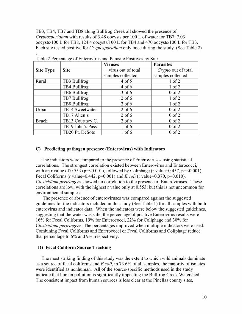
10

TB3, TB4, TB7 and TB8 along Bullfrog Creek all showed the presence of Cryptosporidium with results of 3.48 oocysts per 100 L of water for TB7, 7.03 oocysts/100 L for TB8, 124.4 oocysts/100 L for TB4 and 470 oocysts/100 L for TB3. Each site tested positive for Cryptosporidium only once during the study. (See Table 2) . Table 2 Percentage of Enterovirus and Parasite Positives by Site Viruses Parasites Site Type Site + virus out of total

samples collected + Crypto out of total samples collected

Rural TB3 Bullfrog 4 of 5 1 of 2 TB4 Bullfrog 4 of 6 1 of 2 TB6 Bullfrog 3 of 6 0 of 2 TB7 Bullfrog 2 of 6 1 of 2 TB8 Bullfrog 2 of 6 1 of 2 Urban TB14 Sweetwater 2 of 6 0 of 2 TB17 Allen’s 2 of 6 0 of 2 Beach TB13 Courtney C. 2 of 6 0 of 2 TB19 John’s Pass 1 of 6 0 of 2 TB20 Ft. DeSoto 1 of 6 0 of 2 C) Predicting pathogen presence (Enterovirus) with Indicators The indicators were compared to the presence of Enteroviruses using statistical correlations. The strongest correlation existed between Enterovirus and Enterococci, with an r value of 0.553 (p=<0.001), followed by Coliphage (r value=0.457, p=<0.001), Fecal Coliforms (r value=0.442, p=0.001) and E.coli (r value=0.370, p=0.010). Clostridium perfringens showed no correlation to the presence of Enteroviruses. These correlations are low, with the highest r value only at 0.553, but this is not uncommon for environmental samples. The presence or absence of enteroviruses was compared against the suggested guidelines for the indicators included in this study (See Table 1) for all samples with both enterovirus and indicator data. When the indicators were below the suggested guidelines, suggesting that the water was safe, the percentage of positive Enterovirus results were 16% for Fecal Coliforms, 19% for Enterococci, 22% for Coliphage and 30% for Clostridium perfringens. The percentages improved when multiple indicators were used. Combining Fecal Coliforms and Enterococci or Fecal Coliforms and Coliphage reduce that percentage to 6% and 9%, respectively. D) Fecal Coliform Source Tracking The most striking finding of this study was the extent to which wild animals dominate as a source of fecal coliforms and E.coli, in 73.6% of all samples, the majority of isolates were identified as nonhuman. All of the source-specific methods used in the study indicate that human pollution is significantly impacting the Bullfrog Creek Watershed. The consistent impact from human sources is less clear at the Pinellas county sites,

11

although there were days when “spikes” of human isolates dominated the sites. The percentage of isolates identified as human by antibiotic resistance analysis was significantly correlated with enterovirus counts, but the percentage of isolates identified as human by ribotyping was not significantly correlated with enterovirus counts. This discrepancy points to the need for including the fingerprints of more isolates from known, local sources in the respective databases.

E) Climate and Indicators The Fall peak in fecal indicator levels corresponded to the end of the rainy season, however, the Spring peak could not be linked to rainfall or stream flow parameters. A lag time beyond 30 days existed when rainfall was compared to the indicators, but localized peaks associated with rainfall events may still occur within individual watersheds. Total rainfall rather than average rainfall was better than stream flow for predicting indicator level peaks overall. For Enterococci, the 7 day total rainfall value was useful, but for coliphage, the 3 day total was better perhaps because of the decreased survival of this indicator in warm tropical waters. Average rainfall for beach sites was useful only when looking widely at the Bay, not for the individual sites. Enterococci compared to the 10 day total rainfall value was the only useful indicator correlation at the beach sites. Negative correlations to rainfall and stream flow suggest that in some watersheds dilution due to increased rainfall and stream flow will actually decrease the number of phage and Clostridium. Both coliphage and Clostridium were found in low numbers compared to the other indicators. Sources are more likely to be related to feces compared to coliforms and Enterococci, which might have a soil or vegetative source. And while Clostridium could accumulate in sediments and does survive for extended periods of time, the low concentrations make it susceptible to non-detects when fresh water increases. Binary Logistic Regressions were used to determine the relationship between rainfall, stream flow and the presence of Enterovirus. A slightly significant logistic regression result occurred within the beach site grouping between the 7 day average rainfall values and the presence of Enterovirus, resulting in a 64.3% concordant percentage, 30.4% discordant percentage and a 5.4% tie. Salinity and Enterovirus in this same beach grouping resulted in a concordant percentage of 69.6%, 26.8% discordant percentage and a 3.6% tie. No other significant relationship was found between the climate factors used in the study, and the presence or absence of Enterovirus. The virus data set for this study is small, however, and a more intensive virus sampling regime may be needed for a more accurate statistical analysis of climate factors and their contribution to virus water quality on the beaches.

12

V. Recommendations What indicators are appropriate for Tampa Bay? • The use of two indicators, both the fecal coliform bacteria and enterococci on a

routine basis is warranted based on the results of this study. E.coli appears to be of little added value in either marine or fresh waters.



• Clostridium perfringens and Bacteroides phage, while indicative of fecal pollution, only have limited added value as alternative indicators.


and septic tank inputs into common warm marine waters. • Biological Source Tracking is a very useful tool, and a large database for Tampa Bay

should be built and supported. The continued use of fecal coliform bacteria is supported but only with the addition of enterococci, as well as characterization of the types of fecal coliform bacteria found using the source tracking techniques. Coliphage as a third indicator should be added during specialized surveys. This approach will be useful in demonstrating risk, seasonal variability, sources and the data can be used to make both short-term and long-term management decisions on the watershed. What levels are appropriate for Tampa Bay? • The 104 CFU single sample level and geometric mean of 35 CFU associated with

Enterococci is partially supported by this study for the fresh water tributaries. However the 200 and 800 CFU for the fecal coliform bacteria are not and may be too stringent. A set of values for the fecal coliform bacteria can not be supported at this time.

• A greater database is needed at the contrasting beaches to make recommendations for beach water quality monitoring and levels.

Is pathogen monitoring warranted? • Viruses have been the group of pathogens which have shown the most value in



13




Are the data and recommendations for Tampa Bay useful for a State-wide program? • Yes, state, local and private agencies involved in water quality studies (wastewater,

stromwater, septage etc), should move immediately to monitoring for both enterococci and fecal coliform bacteria as well as contributing to a state-wide database on the characterization of “source-tracking” isolates. Virus testing should be built into specialized studies.

Perspective and Future Directions: Healthy Beaches Phase II and beyond Because most pathogens are host-specific, the goal of this study has been to access the risk of human disease by measuring pollutants of human origin. However, a great deal of additional work remains in order to protect public health and enhance the environment, including: • Modeling of conditions that determine pollution events to provide ways to predict,

avoid and mitigate. Healthy Beaches Phase II has been proposed to address modeling and risk assessment. (Proposal is included in Appendix XII)

• Development of technology and methods such as biosensors to enable the rapid measurement of indicators or actual pathogens.

• Better understanding and response to waterborne diseases not necessarily of human origin, such as those that cause wound infections, animal parasites such as Giardia and Cryptosporidium, organisms from animal waste (e.g. E.coli 0157:H7), and natural organisms such as Vibrio vulnificus and harmful algal blooms.

• Development of a comprehensive database of Enterococci and Fecal Coliforms for use in biological source tracking, and development of methods to quickly perform the analysis locally.

• Increase efforts to eliminate or reduce identified causes of pollution, such as septic tanks, leaking sewer collections systems, failing lift stations, provision of sanitary facilities at beaches, and selected sources of animal pollution.

• Develop statutes, guidelines, methods and education programs so that the public will be aware of risks and take action accordingly as it is not possible to obtain a natural environment that is entirely risk free.

• Undertake a risk assessment investigation specific to warm climates areas, including epidemiological methods, to quantify the relationship between exposure to various concentrations of pathogens and the associated risk of acquiring disease.

111

Appendix I DETERMINING THE EFFECTS OF EL NINO-SOUTHERN OSCILLATION ON COASTAL WATER QUALITY Erin K. Lipp1,2, Nancy Schmidt, Mark E. Luther and Joan B. Rose University of South Florida, College of Marine Science 140 7th Ave. S St. Petersburg, FL 33701 TEL: 727 553 1130

*Corresponding author § Present Address: Center of Marine Biotechnology University of Maryland Biotechnology Institute 701 E. Pratt St. Baltimore, MD 21202 TEL: 410 234 8887 [email protected] Abstract

The importance of El Niño-Southern Oscillation on regional-scale climate variability is well recognized; however the associated effects on local weather patterns are poorly understood. Little work has addressed the ancillary impacts of climate variability at the community level, which require analysis at a local scale. In coastal communities water quality and public health effects are of particular interest. Here we describe the historical influence of ENSO on coastal water quality in Tampa Bay, Florida (USA) as a test case. Using approximate randomized statistics, we show significant ENSO influences on water quality, particularly during winter months, with significantly greater fecal pollution levels during strong El Niño winters and significantly lower levels during strong La Niña winters as compared to neutral conditions. Significant patterns were also noted for El Niño and La Niña falls. The success of the analyses in this test case demonstrates the feasibility of assessing local effects associated with large-scale climate variability in any area and highlight the possibility of using ENSO forecasts to predict periods of poor coastal water quality in urban regions. Introduction

The link between climate and health was recognized as early as the 16th century (Rees 1996). Without knowledge of disease-causing agents, many believed that strange weather patterns caused a variety of health problems, resulting in the adage, “under the weather” (Rees 1996). While it has long been long realized that “bad airs” do not cause disease, in recent years there has been increased scientific recognition that climate change and variability contribute to the distribution, growth and survival of certain pathogenic microorganisms and, therefore, impact public health (Colwell 1996; Checkley et al. 2000; NOAA 1999). Both local weather patterns and climate variability play a role in the dispersion of pathogenic microorganisms. Events such as extreme rainfall and floods often overburden water treatment facilities and onsite disposal systems and increase storm water run-off; all of which may result in the introduction of high levels of enteric pathogens to nearby surface waters and wells. Interannual climate variability due to El Niño-Southern Oscillation (ENSO)

112

and other phenomena also affects water quality and public health both directly and indirectly by resulting in poor sanitation due to floods (Gueri et al. 1986) or promoting favorable conditions for growth/survival of certain pathogens, i.e. Vibrio cholerae (Colwell 1996). Also, given the importance of non-point sources of pollution in the United States and elsewhere, heavy or prolonged rains may contribute to pollutant loading, including pathogenic microorganisms, from urban and agricultural run-off and on-site sewage disposal (O’Shea and Field 1992; Paul et al. 1997). Exposure to the public during these events occurs from the contamination of drinking water, recreational water and shellfish (Rose 1997).

Short-term predictive models forecast ENSO events with varying success rates and research has effectively demonstrated a strong relationship between regional precipitation patterns and ENSO (Ropelewki and Halpert 1986; Schmidt et al. in review). In addition to the importance and utility of regional-scale models, an understanding of anomalies in local weather patterns is an important and immediate concern. However, there has been little work to demonstrate statistically significant weather patterns, or determine the ancillary effects of these anomalies related to ENSO at the local scale. This contribution builds upon previous research by the authors on the topic of ENSO influence on local variability in seasonal rainfall and river discharge in Florida. Using an approximate randomized difference of means test, Schmidt et al. (in review) demonstrated significant seasonal responses of rainfall and streamflow to El Niño and La Niña conditions in south central Florida. The study also found significant seasonal variability in rainfall within the state of Florida, with distinct patterns noted particularly between the panhandle and southernmost Florida.

We hypothesize that a statistical relationship may exist between ENSO and water quality given reported relationships between ENSO, precipitation and river discharge (Sun and Furbish 1997; Zorn and Waylen 1997) and the subsequent relationship between water quality and both rainfall and discharge (Barbé and Francis 1995). Using historical data, we analyzed the relationship between microbiological water quality and ENSO in south central Florida, a region that is known to experience anomalous precipitation and river flow associated with ENSO phases (Schmidt et al. in review). The strength of these relationships and seasonal changes were evaluated with analyses of continuous and categorical data. Here we demonstrate a simple approach to define the role of particular modes of climate variability (i.e., ENSO) on coastal water quality by focusing on temporal and spatial scales that are important to public health decisions at local levels using Tampa Bay, FL (USA) as a test case. Materials and Methods Description of Study Site

Historical changes in water quality and their relationship to ENSO were assessed in Tampa Bay, FL. Tampa Bay is the second largest Gulf Coast estuary and the largest estuary in Florida. The entire watershed contains 35,500 km2, which are drained by 31 major basins (SWFWMD 1998). We studied seven drainage basins (Fig. 1), which are qualitatively described in terms of major land-use patterns and other sources of pollution in Table 1. Currently, within the entire Tampa Bay watershed 56% of the land is developed; 40% of the built-up areas are urban and 16% include agricultural and pasture lands (SWFWMD 1998). El Niño-Southern Oscillation Indices

The ENSO state was measured using the Climate Prediction Center’s Niño Region 3.4 monthly Sea Surface Temperature anomaly (SSTA) indices, which are based on recorded temperatures from 5 oN to 5 oS and 170 oW to 120 oW in the equatorial Pacific Ocean. Seasons from 1974-1998 were classified as extreme or neutral. Seasons were defined as follows: winter included January, February and March; spring included April, May and June; summer included July, August and September; and fall included October, November and

113

December. ENSO extreme seasons were defined to occur when the five-month running average, centered on the season, of the Niño Region 3.4 SSTA exceeded ± 0.7 oC. Neutral ENSO seasons were defined to occur when the five-month running average, centered on the season, fell between ± 0.4 oC (Tbl. 2). These thresholds excluded questionable ENSO events while providing an adequate number of cases for analyses for all ENSO phase seasons for all seasons except extreme La Niña spring. Where data were available there was often a strong signal noted in extreme La Niña springs. Therefore, for those cases where insufficient data existed for extreme La Niña, all La Niña springs, including weak (-0.40 to -0.69 oC) episodes, were tested.

Monthly water quality data (1974–1998) were obtained for Tampa Bay and its tributaries from the Hillsborough County Environmental Protection Commission (HEPC). Water quality was quantitatively assessed using concentrations of fecal coliform bacteria (colony forming units (CFU)/100 ml) at 29 stations. Concentrations for each sample were transformed by the equation, log10 (CFU/100 ml) + 1, to obtain a normal distribution. When concentrations were below detectable limits (<1 - <100 CFU/100 ml), a value of zero was used for statistical analyses. Samples were collected only once per month from each station. Consequently, stations were combined in individual watersheds to mitigate small-scale events that might dominate a local area during the monthly sampling but would not be indicative of an entire drainage basin. In all, seven drainage basins were examined and included an average of 4.1 stations per watershed. A maximum of 7 and a minimum of 2 stations were used per drainage basin.

Approximate randomized statistics were used in all analyses. These computer-intensive tests generate the probability distribution of the test statistic by recomputing it for many (>100) artificially constructed data sets and can be used to assess significance under minimal assumptions. The observations that are tested do not need to meet the normal distribution criteria of conventional parametric statistics; likewise they need not constitute a random sample. In addition to avoiding the assumptions required of parametric statistics, approximate randomized tests maximize the ability to discriminate between hypotheses because the sampling distribution is known (Noreen 1989).

In order to perform correlation analyses against Niño Region 3.4 SSTA, anomalies in fecal coliform levels were obtained by subtracting the basin-averaged mean monthly value (over the data record) from individual basin-averaged monthly values. Significance of the Pearson correlation coefficients was determined by comparing the r-value of the observed correlation to that of the distribution of the correlation under the null hypothesis. This distribution was generated by randomly shuffling the SSTA values against fecal coliform anomaly values and recalculating the r-value 10,000 times. Correlations were run against the entire data record, with a lag of zero to three months between monthly Niño Region 3.4 SSTA and monthly water quality anomalies to allow the detection of any delayed responses.

The correlation test provides information regarding the significance of the relationship between ENSO and fecal coliform levels but does not reveal details concerning the relative importance of particular seasons. Therefore, the differences in mean fecal coliform concentrations between extreme El Niño, neutral and extreme La Niña events for each season were analyzed using an approximate randomized difference of means test (Noreen 1989). Log-transformed basin-averaged seasonal fecal coliform concentrations for extreme El Niño and La Niña events were tested against the seasonal fecal coliform levels for neutral periods. The observed difference in means was compared to the distribution of the randomly generated difference under the null hypothesis. As in the correlation analysis, recalculating the difference in means 10,000 times generated the distribution. Given the high level of noise inherent in the fecal coliform data set and the need to average over time and space, results were considered to be statistically significant at an α level of 0.10 rather than 0.05.

114

Results Correlation Analysis

Work by Schmidt et al. (in review) indicates that both precipitation and streamflow in south central Florida are significantly related to ENSO. Given that water quality often deteriorates during periods of high precipitation and river discharge, we hypothesized that a direct relationship may exist between ENSO state and water quality. Fecal coliform bacteria were used as a proxy for water quality, as they are the most commonly used indicator of poor water quality due to fecal pollution and potential health risks world-wide. Correlation analyses were used to provide an initial assessment of whether any relationship existed between Niño 3.4 SSTA (ENSO state) and changes in fecal coliform levels (water quality) in Tampa Bay.

Analysis of monthly anomalies in fecal coliform levels with monthly Niño 3.4 SSTA revealed a significant and positive correlation in five of the seven watersheds examined over the 25-year period of record. In general, even for significant correlations, coefficients were low (r = 0.088 to 0.23). However, these values were similar to those obtained for comparisons between Niño 3.4 SSTA and both precipitation and streamflow in Florida (Schmidt, N. unpublished data). The majority of basins with strong correlations were located in the eastern portion of the Tampa Bay watershed. In this region, land use includes broad areas devoted to agriculture and pasture. Furthermore, there is substantial land application of sewage sludge in some areas (SWFWMD 1998; Tbl. 1). Land use appears to be an important factor in relating changes in water quality to the strength of ENSO.

Seasonal Analysis

The importance of the ENSO phenomenon to variability in factors such as rainfall and streamflow in Florida, and elsewhere, varies with season (Schmidt et al. in review). Therefore, given the significant relationship for most of the studied watersheds between fecal coliform levels and Niño 3.4 SSTA, we expanded our examination to assess the seasonal differences in fecal coliform levels between extreme ENSO phases (El Niño and La Niña; Tbl. 2) and neutral conditions to better define the relationship between ENSO state and water quality. Basin-averaged fecal coliform values were compared between seasons and ENSO phase.

Winter. Fecal coliform levels were compared between neutral winters and both extreme El Niño and extreme La Niña winters (Fig. 2). For extreme El Niño winters, there was an overall increase in fecal coliform levels as compared to neutral. With the exception of Delaney Creek, where the percent deviation was –20.4 (P = 0.087), the deviations in fecal coliform levels from neutral ranged between 7.6% and 18.7%. However, only at Rocky and Sweetwater Creeks were the fecal coliform levels significantly greater than neutral values (P < 0.10). During extreme La Niña winters, there was an overall decrease in fecal coliform levels as compared to neutral winters. With the exception of Rocky Creek, where the percent deviation from neutral was 36.8 (P = 0.034), the deviations in fecal coliform levels from neutral ranged between –16.2% and –45.5%. Fecal coliform levels at Bullfrog Creek, Delaney Creek, Hillsborough River, and Sweetwater Creek were significantly below neutral values (P < 0.05). Fecal coliform levels at Little Manatee River were significantly lower than neutral at P <0.10. Although Alafia River fecal coliform values showed a negative deviation during extreme La Niña winters, the difference from neutral was not significant.

115

Spring. For extreme El Niño springs, the average fecal coliform levels were lower than those found during neutral springs (Fig. 2). Percent deviations from neutral ranged between –4.6 and –20.1; however, differences were not significant in any watershed. For the one case of an extreme La Niña spring, fecal coliform levels in all basins were significantly below neutral values (P < 0.10). Deviations from neutral ranged from -0.9% to -46.0%. Given the lack of data during extreme La Niña spring events, deviations from neutral were also examined for all five spring La Niña events. For the more general La Niña springs cases, levels in all basins were lower than during neutral spring (-2.1% to -47.4% deviation). However, the differences were not significantly different from neutral values.

Summer. Fecal coliform levels during extreme El Niño summers showed a varied response with neutral values (Fig. 2). None of the fecal coliform concentrations were significantly different than levels found in neutral summers and percent deviations ranged from –13.7 to 11.8. For extreme La Niña summers, percent deviations were consistently negative (-0.1% to -45.1%). However, the differences from neutral were not significant.

Fall. Fecal coliform concentrations during extreme El Niño falls were generally greater than that found during neutral periods (Fig. 2). Although fecal coliform values at Bullfrog Creek, Delaney Creek and Little Manatee River were less than that found during neutral fall, the differences were not significant. The remaining stations all showed greater than neutral fecal coliform concentrations, with deviations between 8.2% and 25.3%. The difference from neutral was only significant for Hillsborough River (25.3% deviation) and Rocky Creek (22.3% deviation). Patterns during extreme La Niña falls showed both positive and negative deviations from neutral. The only drainage with significant differences from neutral was the Little Manatee River, where levels were 17.5% below neutral values.

Discussion

Extreme weather conditions including droughts and floods can dramatically affect communities at many levels. Direct effects may include crop damage, property damage, destruction of homes and loss of life. However, even moderate changes in climate can affect water resources in both quantity and quality and thus indirectly affect public health. Although research has demonstrated regional-scale climate variability during ENSO phases, particularly relating to changes in temperature and precipitation (Ropelewski and Halpert 1986; Livezey et al. 1997; Gershunov and Barnett 1998; Livezey and Smith 1999), it is at the local level where economic and public health impacts are felt and where decisions regarding public policy must be made. Consequently, there is a need to better predict and understand the effects of climate variability at the local scale. To our knowledge this is the first study to examine the ancillary or indirect effects of ENSO on fecal pollution in coastal waters as it relates to recognized changes in precipitation and streamflow.

The extreme El Niño conditions observed in 1997 and early 1998 spurred investigations into the effects of climate variability on human health (NOAA 1999). During this time, the role of rainfall and streamflow in the introduction and transport of indicators of fecal pollution and human enteroviruses to coastal waters was demonstrated in southwest Florida (Weiskel et al. 1996). Higher than average precipitation and subsequent river discharge were found in the winter months (1997 – 1998) along with lower water temperatures. Those patterns, which are typical of El Niño winters, provided a mechanism for transport of enteric contaminants by run-off and discharge into coastal waters and increased survival due to lower salinity and temperature (Barbé and Francis 1995; Wyer et al. 1995; Weiskel et al. 19996; Sun and Furbish 1997).

Throughout Florida and in the Tampa Bay area, tremendous population growth in the last 20 years has been accompanied by an increased volume of wastewater discharged to coastal waters. Furthermore, non-point sources (from septic systems and stormwater run-off) constitute a major cause of coastal pollution. Factors such as agricultural lands, land

116

application of sewage sludge, septic systems and wildlife contribute to high levels of coastal fecal pollution when transport mechanisms, such as high precipitation and river discharge, are in operation. The consequences of such pollution include closures of recreational and shellfish propagating waters and potential exposure to human pathogens (Lipp and Rose 1997).

The predictable, or “normal,” seasonal nature of rainfall in Florida has lead to specific water management strategies. The majority of rainfall in southern and central Florida occurs in the summer months, while spring and fall are relatively dry. In the southern part of the state winter storms account for less than 15% of the average annual precipitation (Nese and Grenci 1996). Similar to the larger-scale patterns noted for the southeastern United States (Ropelewski and Halpert 1986) precipitation and consequently streamflow along the south central Gulf coast of Florida are strongly related to ENSO (Schmidt et al. in review). The seasonal ENSO effects results in precipitation patterns that are superimposed upon the normal seasonal trends. Significant correlations between ENSO (using Niño 3.4 SSTA) and fecal coliform levels at the majority of basins analyzed demonstrate that Tampa Bay water quality also may be broadly linked to the ENSO state via teleconnections that results in anomalous precipitation and river discharge. Significantly increased fecal pollution, relative to neutral conditions, was most dramatic for extreme El Niño winter months. ENSO development tends to peak in the winter; consequently the strongest weather patterns are also noted during that time (Ropelewski and Halpert 1986). Significant increases in wintertime precipitation and discharge in Florida during extreme El Niño events (Zorn and Waylen 1997; Schmidt et al. in review) may exacerbate conditions and result in greater than average levels of indicator organisms or introduction of enteric pathogens (Lipp et al. in review). Conversely, below average precipitation and discharge (Schmidt et al. in review) lead to depressed fecal coliform levels during extreme La Niña winters. A significant ENSO signal was also often noted in the fall, and the signal was generally variable, although not significant, in the spring. The ENSO signal was ambiguous in the summer. In general, these observations follow patterns noted for both precipitation and river discharge in south central Florida (Schmidt et al. in review) (Fig. 2). This type of information will be useful in proactively tailoring water quality monitoring and control programs in the Tampa Bay region.

Conclusion

In this historical assessment, changes in water quality (using fecal coliform bacteria) in Tampa Bay, FL were shown to vary with ENSO phases. We have previously shown a significant relationship between ENSO and precipitation and discharge (Schmidt et al. in review) and between water quality and rainfall and discharge in Florida (Lipp et al. in review), and now report that a direct association between fecal pollution and ENSO can be measured. Despite an inherently noisy data set, significant trends between fecal coliform levels and Niño 3.4 SSTA were noted for the majority of the Tampa Bay watersheds we examined. This study provides a baseline to initiate the development of water quality “forecast” models, ultimately using factors such as ENSO and other climatic variables combined with land-use characteristics to predict periods of poor water quality. This will further the development of public policies for monitoring, assessing and managing important bays and coastlines for recreation, industry and fisheries.

117

Literature Cited Rees, R. 1996. Under the weather: climate and disease, 1700 – 1900. History Today 46: 35 –

41. Checkley, W., L.D. Epstien, R.H. Gilman, D. Figueroa, R.I. Cama, J.A. Patz, and R.E. Black.

2000. Effects of El Niño and ambient temperature on hospital admissions for diarrhoeal diseases in Peruvian children. Lancet 335: 442 – 450.

Colwell, R.R. 1996. Global climate and infectious diseases: The cholera paradigm. Science 274: 2025 – 2031.

NOAA, Office of Global Programs. 1999. An Experiment in the Applications of Climate Forecasts: NOAA-OGP Activities Related to the 1997-98 El Niño Event. NOAA, US Dept. of Commerce. Washington, DC.

Gueri, M., C. Gonzalez, and V. Morin. 1986. The effect of the floods caused by “El Niño” on health. Disasters 10: 118 – 124.

O’Shea, M.L. and R. Field. 1992. Detection and disinfection of pathogens in storm-generated flows. Canadian Journal of Microbiology 38: 267 – 276.

Paul, J.H., J.B. Rose, S. Jiang, X. Zhou, P. Cochran, C. Kellogg, J.B. Kang, D. Griffin, S. Farrah, and J. Lukasik. 1997. Evidence for groundwater and surface marine water contamination by waste disposal wells in the Florida Keys. Water Research 31: 1448 – 1454.

Rose, J.B. 1997. Climate forecasting, water resources and environmental health: Impact of El Niño associated with climate-sensitive diseases. Florida Journal of Environmental Health August: 8 – 13.

Ropelewski, C.F. and M.S. Halpert. 1986. North American precipitation and temperature patterns associated with El Niño/Southern Oscillation (ENSO). Monthly Weather Review 114: 2352 – 2362.

Sun, H. and D.J. Furbish. 1997. Annual precipitation and river discharges in Florida in response to El Niño and La Niña sea surface temperature anomalies. Journal of Hydrology 199: 74 – 87.

Zorn, M.R. and P.R. Waylen. 1997. Seasonal response of mean monthly streamflow to El Niño/Southern Oscillation in north central Florida. Professional Geographer 49: 51-62.

Barbé, D.E. and J.C. Francis. 1995. An analysis of seasonal fecal coliform levels in the Tchefuncte River. Water Resources Bulletin 31: 141 – 146.

Southwest Florida Water Management District (SWFWMD). 1998. Comprehensive Watershed Management Plan, Tampa Bay/Anclote River. Volume 1. Assessment. Technical Report, SWFWMD, Tampa, FL.

Gershunov, A. and T.P. Barnett. 1998. ENSO influences on intraseasonal extreme rainfall and temperature frequencies in the contiguous United States: observations and model results. Journal of Climate 11: 1575 – 1586.

Livezey, R.E., M. Masutani, A. Leetmaa, H. Rui, M. Ji, and A. Kumar. 1997. Teleconnective response of the Pacific-North American region atmosphere to large central equatorial Pacific SST anomalies. Journal of Climate 10: 1787 – 1820.

Livezey, R.E. and T.M. Smith. 1999. Covariability of aspects of North American climate with global sea surface temperatures on interannual to interdecadal timescales. Journal of Climate 12: 289 – 302.

Weiskel, P.K., B.L. Howes, and G.R. Heufelder. 1996. Coliform contamination of a coastal embayment: sources and transport pathways. Environmental Science and Technology 30: 1872 – 1881.

Wyer, M.D., D. Kay, G.F. Jackson, H.M. Dawson, J. Yeo. and L. Tanguy. 1995. Indicator organism sources and coastal water quality: a catchment study on the Isle of Jersey. Journal of Applied Bacteriology 78: 290 – 296.

118

Lipp, E.K. and J.B. Rose. 1997. The role of seafood in foodborne diseases in the United States of America. Revue Scientifique et Technicale. Office Internationale des Epizooties 16: 620 – 640.

Nese, J. and L. Grenci. 1996. The climatology of Florida. In A World of Weather: Fundamentals of Meteorology. Kendall/Hunt Publishing Co., Dubuque, IA.

Noreen, E.W. 1989. Computer Intensive Methods for Testing Hypotheses. John Wiley and Sons, NY.

Unpublished Materials

Lipp, E.K., R. Kurz, R. Vincent, C. Rodriguez-Palacios, S. Farrah and J. B. Rose. In review. Seasonal variability and weather effects on microbial fecal pollution and enteric pathogens in a subtropical estuary. Estuaries.

Schmidt, N., E.K. Lipp, J.B. Rose, M.E. Luther. In second review. ENSO influences on seasonal rainfall and river discharge in Florida. Journal of Climate.

119

Table 2. Classification of ENSO events between seasons, based on period of record available for water quality (1974 – 1998).

Season Extreme El Niño Neutral Extreme La Niña

Winter J F M

1983, 1987, 1992, 1995, 1998

1979, 1981, 1982, 1990, 1991, 1994, 1997 1974, 1976, 1985, 1989

Spring A M J

1982, 1983, 1987, 1992, 1993, 1997

1976, 1977, 1978, 1979, 1980, 1981, 1984, 1986, 1990, 1994, 1995, 1996, 1998

1988 (1974, 1975, 1985, 1989)a

Summer J A S 1982, 1987, 1991, 1997

1978, 1979, 1980, 1981, 1983, 1984, 1985, 1989, 1990, 1992, 1995, 1996

1975, 1988, 1998

Fall O N D

1976, 1977, 1982, 1986, 1987, 1991, 1994, 1997

1978, 1980, 1981, 1985, 1989, 1992, 1996

1975, 1984, 1988, 1995, 1998

a weak La Niña events (Niño 3.4 SSTA -0.4 – -0.69) are included in parentheses

120

Figure 1. Map of Tampa Bay watersheds. Filled circles represent river gage stations, open circles represent water quality stations. BC: Booker Creek, RC: Rocky Creek, SC: Sweetwater Creek, CC: Cypress Creek, HR: Hillborough River, DC: Delaney Creek, AR: Alafia River, BFC: Bullfrog Creek, LMR: Little Manatee River and MR: Manatee River. Figure 2. Chart shows the percentage of stations with fecal coliform (FC), precipitation (PPT) or discharge (DIS.) values that were significantly greater than or less than that of neutral seasons for extreme El Niño (A) and extreme La Niña (B) events. One full bar represents 100% of stations: no color – difference was not significant, gray – difference was significant at P<0.10, black – difference significant at P<0.05. For spring, all La Niña events were used as there was only one extreme La Niña event within the period of record. Significance results are from Schmidt et al. (in review) and included statewide precipitation stations and streamflow for south central Florida (Charlotte Harbor and Tampa Bay) for 1950 to 1998.

121

-100%

-80%

-60%

-40%

-20%

0%

20%

40%

60%

80%

100% %

of s

tatio

ns g

reat

er o

r le

ss th

an n

eutr

al le

vels

-NS -<0.10 -<0.05

Winter Spring Summer Fall

Ppt

.

Dis

.

F.C

.

Ppt

.

Dis

.

F.C

.

Ppt

.

Dis

.

F.C

.

Ppt

.

Dis

.

F.C

.

Significance

122

-100%

-80%

-60%

-40%

-20%

0%

20%

40%

60%

80%

100% %

of s

tatio

ns g

reat

er o

r les

s th

an n

eutra

l lev

els

-NS -<0.10 -<0.05

Significance

Winter Spring Summer Fall

Ppt

.

Dis

.

F.C

.

Ppt

.

Dis

.

F.C

.

Ppt

.

Dis

.

F.C

.

Ppt

.

Dis

.

F.C

.

123

Table 1. Description of Tampa Bay drainage basins.

Basin Drainage Area (acres) Major Land Use Notes

Hillsborough River 431,742 Agriculture (32%; north & ctl); Urban & Industrial (25%; south)

Springs in upper and lower reaches (1 each), dam and drinking water reservoir

Alafia River 270,000 Agriculture (68%; south); Phosphate Mining (east); Urban & Industrial (north & west)

2 springs; >91% of watershed is developed or altered

Bullfrog Creek 25,758 Agriculture (50%; east), Urban & Residential (12%; west)

Rocky Creek 30,008 Urban (41%; south), Agriculture (north) Several lakes up to 93 acres

Sweet Water Creek 23,896 Urban (69%) 2 large lakes (191 and 283 acres)

Delaney Creek 15,161 Urban (55%)

Little Manatee River 135,046 Forest (38%), Agriculture (84%)

OSDS On-site Sewage Disposal Systems 2 WWTP Wastewater Treatment Plant

124

Figure 1

125

Appendix II

Site Descriptions for Tampa Bay Healthy Beaches 1999-2000

Hillsborough County: TB1 Delaney Creek – U.S. 41 just after 36th street (coming from the north), bridge access only, EPC station 133. Small bridge next to Adams Auto Parts on left hand side of road. TB2 Alafia River – U.S. 41 just before Gibsonton, access from Williams Park dock on right side of road traveling south, upstream of fertilizer plant/industrial area, EPC station. TB3 Bullfrog Creek - #5 – continue south on U.S. 41 to next bridge, access from Anderson’s RV park on left side of road, between Beach Ave and Symmes Road. EPC site 144. TB4 Bullfrog Creek - #4 – turn left at the next blinking yellow traffic light just south of TB3 site and head east on Symmes Road, small dip in road just past I-75. Path to water level from north west corner, EPC station 132. TB5 Alafia River – continue east on Symmes Road and turn left onto S.R. 301/43, next big bridge. TB6 Bullfrog Creek - #3 – go back south on 301, west (right) on Big Bend Road (traffic light) to service road just before interstate. (East Bay), continue west on service road to bridge just before I-75, easy path to water on southwest corner leading under 301 bridge, this is a USGS gauging station and just downstream of cattle/agricultural land. You can also get to service road via Big Bend to Lincoln, then left onto service road. TB7 Bullfrog Creek - #1 –take Big Bend Road back to 301 and turn right (south), then east (left) on C.R.672 (go past correctional institute), Look for large American Flag at Goodson Farms on right side of road, take a right on McGrady Road (south) to end. Mr. Lambert – property owner, site is just upstream of planned stormwater retention/treatment pond, around 1600 acres. TB8 Bullfrog Creek - #2 –back track to 301 and continue south (left turn from 672), look for small bridge (“Big Bullfrog Creek”)between Sumner and Bill Tucker Road, main channel flow is under the bridge.. TB9 Little Manatee River – continue south on S. R. 301 from TB8,just south of Bonita and Saffold Roads, and south of Sun City, on south west side (right side of road) look for canoe sign, dirt road leading under bridge, EPC station 113.

126

Site Descriptions for Tampa Bay Healthy Beaches 1999-2000, con’t

TB10 Little Manatee River – back track north on 301, turn left (west) on 674 (Sun City Center Blvd) and follow west to U.S. 41 and turn left (south). Paradise Mobile Home Park on right just before bridge, easy access from fragment of old bridge. EPC station 112. TB11 Manatee River - continue south on U.S. 41 to Palmetto/Bradenten, (do not follow signs to business U.S.41), small access road on right side before Hernando-DeSoto bridge, access road goes under bridge and comes out on northbound U.S.41.

TB12 Hillborough River – On West Kennedy, left side of road just before large white bridge leading to downtown, (Cresent Place North or University Drive) , access to seawall. Pinellas County: TB13 Courtney Campbell Causeway –Pinellas County side, south beach. (Gulf to Bay/SR60). TB14 Sweetwater Creek –on Memorial Hwy, Creek is just past Waltham Ave, small turn off to right just before bridge, seawall on other side of creek near office bldg. EPC station 104 TB15 Tarpon Lake Bypass Canal – Continue west on 576 Memorial Hwy from TB14, turn left (northwest) on 580 (Hillsborough Ave), this turns into 584 (Tampa Rd), continue past Curlew, there should be a large bridge going over canal. Pull into shopping center parking lot (Shoppes of Boot Ranch, next to Blockbuster Video) just before bridge. TB16 Honeymoon Island – Return to 586(Tampa Road) and go back to Curlew. Turn right onto Curlew and follow road, dead-ends at state park (King Duncan Road). Take main park road to end; no swimming beach, high bird population. . TB17 Allan’s Creek –U.S. 19 South just after Belleair Rd intersection, Orange Blossom Grove parking lot, northwest corner. TB18 Joe’s Creek/Cross Bayou – Continue south on U.S.19 to 694, turn right onto Park Blvd, then left onto U.S.1 or Park/Starkey, first large bridge, pull off just past bridge, seawall in southwest corner.

127

Site Descriptions for Tampa Bay Healthy Beaches 1999-2000, con’t TB19 John’s Pass Beach – Continue south on Park Street to ALT 19 (Bay Pines Blvd/Tyrone/595) and turn right (west), stay to left to 666 to Madeira Beach. Turn left on 699 (Gulf Blvd). 1st major bridge will be John’s Pass, small public beach on south west side of bridge, outside of island. TB20 North Beach, Ft. DeSoto Park – continue south on 699 to 682 (Pinellas Bayway) and turn left, turn right onto 679 to Fort DeSoto Park, turn right at ranger station and sample from north beach near lifeguard station. TB21– stop at 4th Street south near USF coming back to university, between 17th and 18th Ave S., small white bridge on west side of road, good water movement. TB22 Control Site – Middle of Tampa Bay, midwater, EPC station 16.

130

Appendix III GIS Locations of Tampa Bay Sampling Sites Location Location Name Lat Long Lat Min Sec Long Calc

TB-1 Delaney Creek 27-54-55 82-24-06 82.00 24.00 6.00 -82.4017 TB-2 Alafia River Mouth 27-51-36 82-23-05 82.00 23.00 5.00 -82.3847 TB-3 Bullfrog Creek Mouth 27-50-17 82-22-54 82.00 22.00 54.00 -82.3817 TB-4 Bullfrog Creek at Symmes 27-50-07 82-20-46 82.00 20.00 46.00 -82.3461 TB-5 Alafia River at US 301 27-52-10 82-19-35 82.00 19.00 35.00 -82.3264 TB-6 Bullfrog Creek at Big Bend 27-47-31 82-21-07 82.00 21.00 7.00 -82.3519 TB-7 Little Bullfrog Creek 27-44-54 82-16-54 82.00 16.00 54.00 -82.2817 TB-8 Big Bullfrog Creek 27-45-05 82-20-07 82.00 20.00 7.00 -82.3353 TB-9 Little Manatee River at US 301 27-40-17 82-21-09 82.00 21.00 9.00 -82.3525

TB-10 Little Manatee River 27-42-16 82-26-50 82.00 26.00 50.00 -82.4472 TB-11 Manatee River 27-30-24 82-33-48 82.00 33.00 48.00 -82.5633 TB-12 Hillsborough River 27-56-52 82-27-47 82.00 27.00 47.00 -82.4631 TB-13 Courtney Campbell Causeway 27-57-39 82-41-52 82.00 41.00 52.00 -82.6978 TB-14 Sweetwater Creek 27-58-55 82-33-43 82.00 33.00 43.00 -82.5619 TB-15 Lake Tarpon Outfall Canal 28-03-40 82-42-36 82.00 42.00 36.00 -82.7100 TB-16 Honeymoon Island Beach 28-03-40 82-49-43 82.00 49.00 43.00 -82.8286 TB-17 Allens Creek 27-56-13 82-43-51 82.00 43.00 51.00 -82.7308 TB-18 Joe's Creek 27-54-00 82-45-15 82.00 45.00 15.00 -82.7542 TB-19 John's Pass Beach 27-46-50 82-46-59 82.00 46.00 59.00 -82.7831 TB-20 Fort Desoto North Beach 27-38-17 82-44-27 82.00 44.00 27.00 -82.7408 TB-21 Salt Creek 27-45-10 82-38-19 82.00 38.00 19.00 -82.6386 TB-22 Control Site 27-58-16 82-40-25 82.00 40.00 25.20 -82.6737

131

Appendix IV Watershed Descriptions

Manatee

Area: 364.48 square miles, perimeter: 117.11 miles Habitat: Forest Riparian, agricultural/urban riparian Cities: Sarasota/Bradenton, Palmetto, Ellenton Rivers and streams: 3 Lakes: 120 Total number of watershed acres: 2223.8 River and stream miles: 561.6 total river miles, 372.6 perennial river miles Surficial aquifer system: 325 square miles of unconsolidated sand and gravel aquifers in this watershed Physiographic province: Gulf Coastal Lowlands, Desoto Plain and Polk Upland Materials: In the coastal areas, undifferentiated sandsss and shells occur near surface. Phosphatic, sandy carbonates subcrop further inland along the Manatee River. An isolated occurrence of phosphatic sandy clays lies in the center of the watershed. Age: Oligocene to Holocene (30 mya to present) Mineral Resources: shell, sand, limestone and phosphate

Little Manatee

Area: 211.01 square miles , perimeter: 92.7 miles Flow station is at TB10 Habitat: Forest Riparian, agricultural/urban riparian Cities: Ruskin, Sun City Center, Wimauma, Gulf City Rivers and streams: 1 Lakes: 75 Total number of watershed acres: 5142.7 River and stream miles: 235.7 total river miles, 218 perennial river miles Surficial aquifer system: 144 square miles of unconsolidated sand and gravel aquifer in this watershed Physiographic province: Gulf Coastal Lowlands and Polk Upland Materials: In the coastal areas, undifferentiated sands and shells occur at or near surface. Phosphatic, sandy clays occurs toward the center of this watershed, especially along the Little Manatee River. The east half of the area is covered by up to 50 feet of ? Age: Miocene to Holocene (14 mya to present) Mineral Resources: phosphate, shell, quartz sand

132

Alafia

Area: 421.67 square miles , perimeter: 103.77 miles Flow station upstream from TB5 Habitat: Forest Riparian, agricultural/urban riparian Cities: Brandon, Riverview, Gibsonton, Plant City Rivers and streams: 5 Lakes: 370 Total number of watershed acres: 11643.2 River and stream miles: 302.4 total river miles, 298 perennial river miles Surficial aquifer system: 346 square miles of unconsolidated sand and gravel aquifer in this watershed Physiographic province: Polk Uplands and Gulf Coastal Lowlands. Several springs discharge ground water into the Alafia River. Materials: Undifferentiated sands in this area range in thickness from less than five feet to more than 30 feet and contain variable amounts of clay and trace amounts of phosphate. These sands cover sandy carbonates along the Alafia river. In other areas, near-surf? Age: Oligocene to Holocene (30 mya to present) Mineral Resources: phosphate, quartz sand

Hillsborough

Area: 658.32 square miles , perimeter: 149.96 miles Flow station upstream from TB12 Habitat: Forest Riparian, agricultural/urban riparian Cities: Tampa area, Temple Terrace Rivers and streams: 5 Lakes: 327 Total number of watershed acres: 6571 River and stream miles: 480.5 total river miles, 279.4 perennial river miles Surficial aquifer system: 371 square miles with no principal aquifer, 281 sq miles with Florida aquifer system (carbonate-rock aquifers) and 7 sq miles of surficial aquifer system of unconsolidated sand and gravel aquifers Physiographic province: Gulf Coastal Lowlands, Zephyrhills Gap, Polk Upland, Lakeland Ridge, Western Valley Materials: Undifferentiated sands cover much of the area, with limestones along the Hillsborough River and to the northeast along the Hills/Pasco county line. In eastern Hills county, near-surface sediments include phosphate clays. Age: Oligocene to Holocene (30 mya to present) Mineral Resources: phosphate and limestone Hillsborough County pop 940,484 as of July 1999

133

Pinellas County Watershed

Pinellas County is not divided into distinct watersheds, but is rather a pennisula with a series of creeks, wetlands and inter-coastal waterways with non-continuous waterflow. The population as of July 1999 was 878,499. The county covers 264 square miles, and although it is the 2nd smallest county in Florida, it is the most densely developed and populated. All watershed information was obtained from the Environmental Protection Agency’s watershed website: http://www.epa.gov/surf3/states/FL/ and the Pinellas County website: http://www.co.pinellas.fl.us/

134

Appendix V Raw Data Sheets – Physical and Chemical Measurements Tampa Bay Healthy Beaches Project 1999-2000

(ntu) (Degrees C) (ppt)Station Date Time pH Turbidity Temperature Salinity Flow/Tide Information

Jun-99 TB1 06-Jun 8:58 7.31 1.00 26.5 5 slowTB2 06-Jun 9:22 8.13 2.00 28.0 24 no tideTB3 06-Jun 9:45 7.66 4.00 26.0 19 low tideTB4 06-Jun 10:04 7.42 1.75 24.5 0.5TB5 06-Jun 10:26 7.50 2.75 26.5 5TB6 06-Jun 11:00 7.40 1.50 25.0 0.5TB7 06-Jun 11:19 6.97 0.50 24.5 0TB8 06-Jun 11:37 6.82 0.50 24.0 0.5TB9 06-Jun 11:56 6.79 2.00 25.0 0TB10 06-Jun 12:45 7.63 1.50 27.5 19 outgoingTB11 06-Jun 1:15 8.28 3.50 28.0 29 outgoingTB12 22-Jun 7:45 7.53 1.50 28.0 14 high tideTB13 22-Jun 8:35 7.90 4.00 28.0 28 slack tideTB14 22-Jun 8:55 7.83 8.50 26.0 0 slack tideTB15 22-Jun 9:30 7.61 1.25 29.0 0 slack tideTB16 22-Jun 10:00 8.00 5.00 29.0 33 slack tideTB17 22-Jun 10:40 7.39 2.50 29.0 21 slack tideTB18 22-Jun 11:11 7.53 2.00 30.0 10 outgoing high tideTB19 22-Jun 12:00 8.11 4.75 31.0 36 incoming high tideTB20 22-Jun 12:50 8.16 3.75 32.0 35 low tideTB21 22-Jun 13:30 7.80 3.50 32.0 24 outgoing high tideTB22 22-Jun 9:40 8.10 1.50 28.4 31.2 incoming tide

Jul-99 TB1 07-Jul 9:30 6.95 7.50 28.0 0 outgoingTB2 07-Jul 9:50 7.54 2.00 29.0 15 outgoingTB3 07-Jul 10:20 7.44 2.00 29.0 16 flowing inTB4 07-Jul 10:45 7.61 3.00 26.0 2 flowing inTB5 07-Jul 11:00 7.34 1.00 28.0 0 flowing outTB6 07-Jul 11:20 7.35 1.00 26.0 0 flowing outTB7 07-Jul 11:45 6.75 0.50 26.0 2 flowing outTB8 07-Jul 12:05 6.82 0.50 28.0 0 still TB9 07-Jul 12:25 6.80 1.50 27.0 0 still TB10 07-Jul 13:30 6.79 1.50 32.0 5 still TB11 07-Jul 14:05 8.09 2.00 32.0 15 flowing outTB12 20-Jul 6:41 7.39 0.5 30 8 flowing inTB13 20-Jul 9:01 7.9 3.25 31 20 flowing in TB14 20-Jul 7:21 7.35 3 29.5 7 flowing inTB15 20-Jul 7:45 7.77 2 30 0 flowing outTB16 20-Jul 8:17 8.05 3 29 32 flowing in TB17 20-Jul 9:16 7.65 2 30 20 flowing inTB18 20-Jul 9:46 7.59 1.5 32 11 flowing inTB19 20-Jul 10:04 8.1 1 31 31TB20 20-Jul 10:45 8.33 3 32 32TB21 20-Jul 11:25 7.9 4.5 32 24TB22 20-Jul 9:40 31 29.4 incoming tide

A-36

135

Station Date Time pH Turbidity Temperature Salinity Flow/Tide InformationAug-99 TB1 10-Aug 9:35 7.26 3 28 0 high flow

TB2 10-Aug 9:55 7.63 2.5 29 12 incoming-high tideTB3 04-Aug 8:05 7.6 3.5 30 21TB4 04-Aug 7:40 7.4 1.25 27 0TB5 10-Aug 10:20 7.57 5 27 0 high tideTB6 04-Aug 10:08 7.2 1.25 27 0TB7 04-Aug 8:56 7.3 1 26.5 0TB8 04-Aug 7:30 6.9 0.5 28 5TB9 10-Aug 10:45 7.05 4.5 25 0 high waterTB10 10-Aug 11:10 7.4 1.5 30 19 high tide-incomingTB11 10-Aug 11:35 7.8 3 31 17 high tide-incomingTB12 24-Aug 6:43 7.36 1.5 28 3TB13 24-Aug 9:06 8.2 9.5 27 20 high tideTB14 24-Aug 7:25 7.45 6.5 28 2TB15 24-Aug 7:54 7.42 1.25 29 0TB16 24-Aug 8:29 8.12 20 28 33 high tide-strong surfTB17 24-Aug 9:24 7.45 2 27 12 slack tideTB18 24-Aug 9:55 4.25 27.5 2 slack tide-health warningTB19 24-Aug 10:14 8.2 10.25 29.5 34 high tideTB20 24-Aug 11:00 8.23 3.5 31 34TB21 24-Aug 11:40 7.67 2 29 16TB22 24-Aug 9:17 8.16 1.25 29.1 28.3 incoming tide

Sep-99 TB1 07-Sep 9:15 7.35 4 26 0 rainingTB2 07-Sep 9:30 7.82 2.5 29 18 raining,high incoming tideTB3 07-Sep 9:45 7.46 3.5 27 10 raining,high incoming tideTB4 07-Sep 9:55 7.65 5.5 25 0 rainingTB5 07-Sep 10:10 7.5 2.5 27 0 high tideTB6 07-Sep 10:20 7.13 3.75 25 0 high flowTB7 07-Sep 10:40 6.9 2 24.5 0 high flowTB8 07-Sep 10:50 7.1 1 25 0 high flowTB9 07-Sep 11:05 7.13 2.5 24.5 0 high flowTB10 07-Sep 11:50 7.3 1.5 29 16 high/incomingTB11 07-Sep 12:15 7.8 1.5 30 18 high tideTB12 23-Sep 7:55 7.49 1 27 15TB13 23-Sep 9:30 7.89 6 27 22TB14 23-Sep 8:00 7.54 3 27 2TB15 23-Sep 8:35 7.75 2 26 0TB16 23-Sep 9:15 8.01 10 24 33TB17 23-Sep 10:30 7.51 5 27 18TB18 23-Sep 10:05 7.63 4 26 14TB19 23-Sep 7.9 3.5 26 34TB20 23-Sep 8.1 4 25 32TB21 23-Sep 10:45 7.7 2 26 18TB22 28-Sep 9:32 27.1 27.1 outgoing

A-37

136

Station Date Time pH Turbidity Temperature Salinity Flow/Tide InformationOct-99 TB1 05-Oct 9:20 7.3 7 25 0 raining

TB2 05-Oct 9:35 7.4 3 26 8 raining,outgoingTB3 05-Oct 10:00 7.1 15 25 0 high flow,rainingTB4 05-Oct 8:35 7 20 25 0 high flow,rainingTB5 05-Oct 9:50 7.4 3.5 25 0 raining,outgoingTB6 05-Oct 11:15 7.1 10 24 1TB7 05-Oct 10:00 6.6 15 24 1TB8 05-Oct 8:40 7.6 20 24 0TB9 05-Oct 10:20 7.1 8 25 0 raining,high waterTB10 05-Oct 11:05 7.2 2.5 27 10 rainingTB11 05-Oct 11:35 7.5 2.5 28 24 raining,outgoingTB12 26-Oct 7:05 7.42 1.5 21 0TB13 26-Oct 9:25 8 5.5 20 22 very low tideTB14 26-Oct 7:38 7.5 5.5 21 8TB15 26-Oct 8:10 7.8 1 22 2TB16 26-Oct 8:48 7.8 25 19 30 very low tideTB17 26-Oct 9:38 7.7 5 21 20 low tideTB18 26-Oct 10:06 7.5 4 21 14 low tideTB19 26-Oct 10:26 7.9 25 21 34 low tideTB20 26-Oct 11:06 8.1 10 21 36 low tideTB21 26-Oct 11:43 7.7 5 22 20 low tideTB22 26-Oct 9:54 3.5 22.2 26.2 outgoing

Nov-99 TB1 09-Nov 9:30 6.6 2.2 19 0TB2 09-Nov 9:45 7.4 2.4 21 10 low tideTB3 09-Nov 9:55 7.4 2.25 22 8 low tideTB4 09-Nov 10:06 7.5 3 18.5 0 low waterTB5 09-Nov 10:17 7.7 2 22 2 low waterTB6 09-Nov 10:36 7.8 2.5 20 0 low waterTB7 09-Nov 10:46 7.1 0.8 19 0TB8 09-Nov 11:01 6.9 0.33 19 0TB9 09-Nov 11:15 7.1 1.2 19 0 low waterTB10 09-Nov 10:45 6.9 1.5 22 10 low tideTB11 09-Nov 12:10 7.8 5.9 22 24 windyTB12 30-Nov 7:09 8.4 1.25 20 20 incoming tideTB13 30-Nov 9:45 8.3 14 20 24 low tideTB14 30-Nov 7:37 8.5 2.75 18 0 outgoingTB15 30-Nov 8:07 8.1 1.3 21 0 high tideTB16 30-Nov 8:45 7.9 4.5 18 30 low tideTB17 30-Nov 10:06 8.1 3.4 19 23 low tideTB18 30-Nov 10:35 7.8 4.1 21 22 low tideTB19 30-Nov 10:55 8 7.5 21 35 mid tideTB20 30-Nov 11:30 8.1 4.9 21 36 low tideTB21 30-Nov 12:10 7.7 4.75 21 26 very low tideTB22 30-Nov 9:30 20.5 28.8 outgoing

A-38

137

Station Date Time pH Turbidity Temperature Salinity Flow/Tide InformationDec-99 TB1 15-Dec 7.3 4.1

TB2 15-Dec 7.6 3.6TB3 15-Dec 7.6 1.75 low tideTB4 15-Dec 7.6 1.75TB5 15-Dec 8:23 7.5 1.25 20 5TB6 15-Dec 9:00 7.7 1.5 18 0TB7 15-Dec 10:00 7.3 0.6 19 0TB8 15-Dec 11:15 7 0.4 20 0TB9 15-Dec 12:10 7.3 1.4 20 0TB10 15-Dec 13:00 7.6 1.1 24 11TB11 15-Dec 13:35 8 0.9 23 30TB12 15-Dec 7:47 7.6 0.6 20 17 flowing inTB13 15-Dec 10:00 7.8 4.4 20 25 low tideTB14 15-Dec 8:18 7.7 2.4 19 6 flowing inTB15 15-Dec 8:44 7.7 1.25 20 2 flowing outTB16 15-Dec 9:22 8.1 11 19 34 low tideTB17 15-Dec 10:16 7.7 2.4 20 23 low tideTB18 15-Dec 10:36 7.5 2 22 21 flowing inTB19 15-Dec 10:54 8 7.4 20 35TB20 15-Dec 11:33 8.2 3 22 35TB21 15-Dec 12:05 7.5 2.6 21 25TB22 08-Dec 9:30 18.3 29.2 incoming tide

Jan-00 TB1 25-Jan 9:25 1.8 15 0TB2 25-Jan 9:40 4.2 17 16TB3 25-Jan 9:50 7.6 16 5TB4 25-Jan 10:05 4.3 14 0TB5 25-Jan 10:20 11 17 2TB6 25-Jan 10:35 2.7 14 0TB7 25-Jan 10:55 1.3 14 0TB8 25-Jan 11:10 0.3 15 0TB9 25-Jan 11:25 1.1 16 0TB10 25-Jan 12:20 1 17 14TB11 25-Jan 12:45 6.5 17 30TB12TB13TB14TB15TB16TB17TB18TB19TB20TB21TB22 25-Jan 9:27 5.8 16.3 30 outgoing

A-39

138

Station Date Time pH Turbidity Temperature Salinity Flow/Tide InformationFeb-00 TB1 15-Feb 9:44 7.1 1.9 20 2

TB2 15-Feb 9:57 7.9 2.1 20 15TB3 15-Feb 10:07 7.8 6 19 12TB4 15-Feb 10:18 8 3.9 18 2TB5 15-Feb 10:33 7.9 2.6 20 5TB6 15-Feb 10:48 8.1 3.6 19 0TB7 15-Feb 11:13 7.3 1.5 19 1TB8 15-Feb 11:25 7.3 0.4 20 1TB9 15-Feb 11:37 7.6 0.7 19 1TB10 15-Feb 12:45 7.5 1.5 21 16TB11 15-Feb 1:12 7.9 1.1 23 30TB12 22-Feb 8:10 7.6 1.4 24TB13 22-Feb 9:30 7.9 19 19 26 outgoing lowTB14 22-Feb 8:30 7.5 6.5 18 8 outgoing lowTB15 22-Feb 9:24 7.8 1.1 0TB16 22-Feb 9:52 8 5.4 33TB17 22-Feb 10:30 7.5 3 19 16 outgoing lowTB18 22-Feb 11:37 7.7 1.8 21 18TB19 22-Feb 7:50 7.9 4 18 34TB20 22-Feb 9:50 8.1 3.4 18.5 36TB21 22-Feb 10:50 7.5 4.3 17 26TB22 22-Feb 9:34 18.8 29.1 outgoing

Mar-00 TB1 21-Mar 7.4 2.5 10TB2 21-Mar 7.4 2.4 22TB3 21-Mar 7.3 1.5 23 12TB4 21-Mar 7.5 0.9 0TB5 21-Mar 8:45 7.4 2.3 24 5TB6 21-Mar 9:20 7.6 0.7 20.5 1TB7 21-Mar 11:00 6.8 1.1 20 1TB8 21-Mar 11:30 6.9 0.25 23 0TB9 21-Mar 1:20 7.1 2 22 1TB10 21-Mar 1:50 7.4 2.4 24 23TB11 21-Mar 2:20 7.9 2.2 25 32TB12 21-Mar 8:31 7.3 3.1 23 26TB13 21-Mar 10:35 7.4 7.5 26 28TB14 21-Mar 9:00 7.4 1.9 23 15TB15 21-Mar 9:30 7.9 1.1 23 2TB16 21-Mar 9:55 8 21 22 36TB17 21-Mar 10:50 7.6 4 25 26TB18 21-Mar 11:10 7.4 1.9 25 26TB19 21-Mar 3:45 7.9 7.6 24 36TB20 21-Mar 1:51 7.9 10 27 35TB21 21-Mar 3:00 7.6 1.7 25.5 30TB22 21-Mar 9:25 7.8 4 22.4 30.7 incoming

A-40

139

Station Date Time pH Turbidity Temperature Salinity Flow/Tide InformationApr-00 TB1 12-Apr 8:45 7.4 2.2 23 13

TB2 12-Apr 9:00 8 2 22 27TB3 12-Apr 9:10 7.7 3 21 23TB4 12-Apr 9:15 8.2 0.7 19 0TB5 12-Apr 9:30 8.4 11 21 7TB6 12-Apr 9:50 8.6 0.5 20 0TB7 12-Apr 10:10 7.6 2.5 19 0TB8 12-Apr 10:25 7.5 0.4 20 0TB9 12-Apr 10:40 7.9 0.6 19 0TB10 12-Apr 11:00 7.7 1.4 22 24TB11 12-Apr 11:30 8 1.4 23 33TB12TB13 25-Feb 10:00 7.9 35 26.5 30TB14 25-Feb 8 7.5 2.3 26.5 27TB15TB16TB17 25-Apr 11:30 6 4.2 27 25TB18TB19 25-Apr 8:30 8 12 20 36 high tideTB20 25-Apr 10:30 8.1 5 25 36 low tideTB21 12-Apr 12:00 8 1.6 23 31TB22 25-Apr 10:00 7.8 24.4 32.3

May-00 TB1 10-May 10:35 7.2 26 15TB2 10-May 11:00 8 27 30TB3TB4TB5 10-May 11:20 8.3 26 0TB6TB7TB8TB9 10-May 12:00 8.1 24 0TB10 10-May 12:20 7.6 26.5 28TB11TB12 10-May 7:00 7.8 27 30TB13 30-May 9:15 7.6 7 28 31TB14 30-May 8:20 7.2 5.5 27.5 19TB15 10-May 7:45 8.7 27 0TB16 10-May 8:15 8.2 26 36TB17 30-May 10:15 7.4 3.5 29.5 30TB18 10-May 9:15 7.5 27 34TB19 30-May 8:30 8 3 78 38TB20 30-May 10:15 8 4 90 36TB21 10-May 1:10 7.8 27 32TB22 23-May 14:55 27.7 33.6 incoming strong

A-41

140

Station Date Time pH Turbidity Temperature Salinity Flow/Tide InformationJun-00 TB1

TB2TB3TB4TB5TB6TB7TB8TB9TB10TB11TB12TB13 19-Jun 10:00 7.9 4.3 30 30TB14 19-Jun 9:00 6.9 5 27 20TB15TB16TB17 19-Jun 11:15 7.4 4 30 29TB18TB19 19-Jun 7.7 2.5 32 38TB20 19-Jun 7.8 7 30 36TB21TB22

Jul-00 TB1TB2TB3 11-Jul 9:15 7.9 4.25 28 20TB4 11-Jul 11:00 7.5 1.5 30 0TB5TB6 11-Jun 10:25 6.4 0.45 0TB7 11-Jun 9:30 6.2 0.5 0TB8 11-Jun 8:25 6.2 2.5 27 0TB9TB10TB11TB12TB13TB14TB15TB16TB17TB18TB19TB20TB21TB22

A-42

141

Station Date Time pH Turbidity Temperature Salinity Flow/Tide InformationAug-00 TB1

TB2TB3 01-Aug 9:45 6.6 3 27 5 low tideTB4 01-Aug 9:00 6.7 4.5 27 0 low tideTB5TB6 01-Aug 8:50 6.7 1.8 26.5 0TB7 01-Aug 9:55 6.5 0.4 26 0TB8 01-Aug 11:00 6.2 0.4 26 0TB9TB10TB11TB12TB13 08-Aug 9:30 8.1 4.5 30.5 28TB14 08-Aug 8:20 7.2 5.8 28 3TB15TB16TB17 08-Aug 10:20 7.7 3.3 32 25TB18TB19 08-Aug 9:00 7.9 4 31 36TB20 08-Aug 10:00 7.7 3.2 32 36TB21TB22

A-43

142

Appendix VI Results of Traditional and Alternative Indicator Monitoring

Table 1

Fecal Coliform Results Fecal Coliform results are given for each sampling site for all months of the study, and are reported in colony forming units (CFU) per 100 mL of water. The figures in bold show the months that the suggested guideline of 800 cfu/100mL for a single sample was exceeded. TB1: Fecal Coliforms (FC) ranged from 55 to 24,450 cfu/100mL, with 2 months (Oct 99 and Mar 00) of out 12 exceeding the guideline. TB2: FC ranged from <10 to 7415 cfu/100mL, with only 1 month (Mar 00) exceeding the guideline. TB3: FC ranged from 100 to 16,350 cfu/100mL, with 4 months (Aug 99, Oct 99, Nov 99 and Mar 00) exceeding the guideline. TB4: FC ranged from 550 to 174,900 cfu/100mL, with all months except Jun 99, Aug 99 and Apr 00 exceeding the guideline. TB5: FC ranged from 35 to 5300 cfu/100mL, with 5 months (Jun 99, Sep 99, Oct 99, Dec 99 and Mar 00) exceeding the guideline. TB6: FC ranged from 300 to 110,200 cfu/100 mL, with all months except Jun 99, Jul 99, Mar 00 and Aug 00 exceeding the guideline. TB7: FC ranged from 12 to 13,850 cfu/100 mL, with 5 months (Aug 99, Sep 99, Oct 99, Dec 99 and Mar 000 exceeding the guideline. TB8: FC ranged from 90 to 6050 cfu/100 mL, with 2 months (Oct 99 and Dec 99) exceeding the guideline. TB9: FC ranged from 100 to 10,250 cfu/100 mL, with 3 months (Aug 99, Oct 99 and Mar 00) exceeding the guideline. TB10: FC ranged from 10 to 4140 cfu/100 mL, with 2 months (Oct 99 and Mar 00) exceeding the guideline. TB11: FC ranged from <10 to 3890 cfu/100 mL, with only one month (Mar 00) exceeding the guideline. TB12: FC ranged from <10 to 3400 cfu/100 mL, with 4 months (Aug 99, Dec 99, Feb 99 and Mar 00) exceeding the guideline. TB13: FC ranged from 15 to 26,900 cfu/100 mL, with 4 months (Sep 99, Dec 99, Feb 00 and Mar 00) exceeding the guideline. TB14: FC ranged from 80 to 33,150 cfu/100 mL, with all months except Nov 99 and Apr 00 exceeding the guideline. TB15: FC ranged from 35 to 40,000 cfu/100 mL, with only Mar 00 exceeding the guideline.

143

TB16: FC ranged from <4 to 4745 cfu/100 mL, with only Dec 99 exceeding the guideline. TB17: FC ranged from <10 to 23,700 cfu/100 mL, with 7 months (Aug 99, Sep 99, Dec 99, Feb 00, Apr 00, Jun 00 and Aug 00) exceeding the guidelines. TB18: FC ranged from <10 to 3115 cfu/100 mL, with 2 months (Aug 99 and Dec 99) exceeding the guideline. Table 1 con’t TB19: FC ranged from <10 to 13,240 cfu/100 mL, with 2 months (Sep 99 and Dec 99) exceeding the guideline. TB20: FC ranged from <4 to 10,900 cfu/100 mL, with 4 months (Sep 99, Dec 99, Feb 00 and Mar 00) exceeding the guideline. TB21: FC ranged from <10 to 6100 cfu/100 mL, with 3 months (Sep 99, Feb 00 and Mar 00) exceeding the guideline. TB22: FC ranged from <1 to 4, with no months exceeding the guideline. The months of Mar 00 and Dec 99 were the worst in terms of the most sites exceeding the FC guideline, with 15 and 13 sites respectively out of 22. Sep and Oct 99 follow closely behind with 10 sites out of 22 for both months.

146

Reported in CFU/100mlTable 1 Fecal Coliform ResultsStation Jun-99 Jul-99 Aug-99 Sep-99 Oct-99 Nov-99 Dec-99 Jan-00 Feb-00 Mar-00 Apr-00 May-00 Jun-00 Jul-00 Aug-00TB1 160 335 440 225 9050 600 215 400 540 24450 55 65TB2 <10 52 265 15 555 190 140 90 125 7415 <10TB3 590 435 3350 440 16350 3500 380 660 420 9600 100 150TB4 605 980 800 2600 174900 3950 16450 6000 3950 28650 550 50500 5000TB5 1350 175 485 810 5300 440 1230 700 580 2925 650 35TB6 435 580 4100 1210 110200 1750 5050 1080 2150 800 1100 1200 300TB7 175 315 8450 1890 8300 500 13850 430 680 17200 450 490 12TB8 90 130 90 105 1035 200 6050 650 370 140 200 430 320TB9 256.5 280 1500 185 10250 160 495 180 100 4200 200 315TB10 110 270 500 52 985 40 32 20 130 4140 10 16TB11 <10 20 76 56 200 15 4 145 10 3890 10TB12 575 240 940 460 55 15 3050 3400 3200 <10TB13 50 370 270 9550 40 75 900 1100 26900 200 210 15 60TB14 4250 1000 6200 12600 1850 170 33150 10500 5650 80 15100 22500 >3000TB15 335 175 350 320 250 123 100 35 40000 185TB16 <10 16 390 2 56<4 4745 10 5 10TB17 610 310 950 23700 160<10 1690 5700 325 2700 75 5685 2000TB18 185 110 850 330 280<10 3115 70 50 20TB19 15 26 34 13240 80 10 3055 700 70<10 <10 20TB20 <10 <4 166 10900<10 <4 4495 2550 2340<10 <10 12 2TB21 <10 190 325 1050 180 25 5340 6100 4810 190<10TB22 <10 4<1 <4 <4 <2 <4 <4 <2 <2

147

Table 2

E.coli Results E.coli (EC) results are given for each sampling site for all months of the study, and are reported in colony forming units (CFU) per 100 mL of water. The figures in bold show the months that the suggested guideline of 126 cfu/100mL was exceeded TB1: EC ranged from 50 to 24,450 cfu/100 mL, with all months except Dec 99 and Apr 00 exceeding the guideline. TB2: EC ranged from 0.5 to 7415 cfu/100 mL, with 4 months (Aug 99, Oct 99, Nov 99 and Mar 00) exceeding the guideline. TB3: EC ranged from 75 to 16,350 cfu/100 mL, with all months except Dec 99, Apr 00 and Jul 00) exceeding the guideline. TB4: EC ranged from 50 to 174,900 cfu/100 mL, with all months except Dec 99 exceeding the guideline. TB5: EC ranged from 85 to 5300 cfu/100 mL, with all months except Jul 99 exceeding the guideline. TB6: EC ranged from 350 to 110,200 cfu/100 mL, with all months exceeding the guideline. TB7: EC ranged from 175 to 17,200 cfu/100 mL, with all months exceeding the guideline. TB8: EC ranged from 70 to 900 cfu/100 mL, with all months except Jun 99, Jul 99, Aug 99 and Mar 00 exceeding the guideline. TB9: EC ranged from 45 to 10,250 cfu/100 mL, with 6 months (Jun 99, Jul 99, Aug 99, Oct 99, Mar 00 and Apr 00) exceeding the guideline. TB10: EC ranged from 10 to 4140 cfu/100 mL, with 3 months (Jul 99, Oct 99 and Mar 00) exceeding the guideline. TB11: EC ranged from <10 to 3890 cfu/100 mL, with only Mar 00 exceeding the guideline. TB12: EC ranged from 15 to 3200 cfu/100 mL, with all months except Oct 99 and Nov 99 exceeding the guideline. TB13: EC ranged from 10 to 26,900 cfu/100 mL, with 6 months (Jul 99, Sep 99, Feb 00, Mar 00, Apr 00 and May 00) exceeding the guideline. TB14: EC ranged from 80 to 15,100 cfu/100 mL, with all months except Apr 00 exceeding the guideline. TB15: EC ranged from 45 to 235 cfu/100 mL, with 2 months (Jun 99 and Aug 99) exceeding the guideline. TB16: EC ranged from <4 to 4745 cfu/100 mL, with 2 months (Aug 99 and Dec 99) exceeding the guideline. TB17: EC ranged from <10 to 23,700 cfu/100 mL, with all months except Nov 99 and May 00 exceeding the guideline. TB18: EC ranged from <10 to 3115 cfu/100 mL, with 3 months (Jun 99, Aug 99 and Dec 99) exceeding the guideline. TB19: EC ranged from <10 to 13,240 cfu/100 mL, with 3 months (Sep 99, Dec 99 and Feb 00) exceeding the guideline.

148

TB20: EC ranged from <4 to 10,900 cfu/100 mL, with 4 months (Sep 99, Dec 99, Feb 00 and Mar 00) exceeding the guideline. TB21: EC ranged from <10 to 5340 cfu/100 mL, with 6 months (Jul 99, Aug 99, Sep 99, Dec 99, Feb 00 and Mar 00) exceeding the guideline. TB22: EC results were negative for all months.

150

Reported in CFU/100mlTable 2 E.coli ResultsStation Jun-99 Jul-99 Aug-99 Sep-99 Oct-99 Nov-99 Dec-99 Jan-00 Feb-00 Mar-00 Apr-00 May-00 Jun-00 Jul-00TB1 160 335 440 9050 550 50 200 350 24450 300TB2 0.5 30 265 200 190 50 80 75 7415 0TB3 150 435 2150 16350 1500 75 650 190 9600 100 100TB4 605 500 520 174900 3950 50 1900 1400 28650 450 50500TB5 1200 85 485 5300 440 900 550 210 2925 400TB6 435 580 2860 110200 1750 350 800 800 700 750 600TB7 175 200 8450 8300 300 250 680 17200 400 210TB8 90 70 70 900 200 310 220 95 200 170TB9 256 200 750 10250 100 45 120 100 4200 200TB10 110 270 30 650 40 25 20 45 4140 10TB11 <10 8 28 55 15 4 55 5 3890 10TB12 500 180 310 190 50 15 1700 3200TB13 35 305 80 9500 30 60 800 26900 200 135 10TB14 425 900 2300 12600 1100 170 1350 1650 80 15100 6000TB15 150 45 235 85 125 123 90 35TB16 <10 12 205 2 48<4 4745 10 5TB17 610 240 390 23700 140<10 1690 1850 140 650 75 225TB18 170 80 500 125 105<10 3115 60 40TB19 15 20 24 13240 70 10 3055 310 40<10 <10 12TB20 <10 <4 122 10900<10 <4 4495 1850 2340<10 <10 4TB21 <10 130 195 650 90 25 5340 2250 4810 130TB22 <10 <4 <1 <4 <4 <4 <2

151

Table 3

Enterococci Results Enterococci results are given for each sampling site for all months of the study, and are reported in colony forming units (CFU) per 100 mL of water. The figures in bold show the months that the suggested guideline of 104 cfu/100mL for a single sampling was exceeded. TB1: Enterococci (ETC) ranged from 40 to 12,300 cfu/100 mL, with all months except Jun 99, Mar 00 and May 00 exceeding the guideline. TB2: ETC ranged from <4 to 496 cfu/100 mL, with 2 months (Aug 99 and Oct 99) exceeding the guideline. TB3: ETC ranged from 10 to 17,200 cfu/100 mL, with 5 months (Sep 99, Oct 99, Nov 99, Jan 00 and Feb 00) exceeding the guideline. TB4: ETC ranged from 134 to 135,650 cfu/100 mL, with all months exceeding the guideline. TB5: ETC ranged from 2 to 6350 cfu/100 mL, with all months except Feb 00, Mar 00, Apr 00 and May 00) exceeding the guideline. TB6: ETC ranged from 68 to 43,000 cfu/100 mL, with all months except Mar 00 and Apr 00 exceeding the guideline. TB7: ETC ranged from 44 to 31650 cfu/100 mL, with all months except Jun 99 exceeding the guideline. TB8: ETC ranged from 42 to 17,850 cfu/100 mL, with 8 months (Jul 99, Aug 99, Sep 99, Oct 99, Dec 99, Jan 00, Jul 00 and Aug 00) exceeding the guideline. TB9: ETC ranged from 20 to 17,200 cfu/100 mL, with 7 months (Jul 99, Aug 99, Sep 99, Oct 99, Nov 99, Dec 99 and Jan 00) exceeding the guideline. TB10: ETC ranged from 10 to 2905 cfu/100 mL, with 3 months (Jul 99, Oct 99 and May 00) exceeding the guideline. TB11: ETC ranged from <4 to 102 cfu/100 mL, with no months exceeding the guideline. TB12: ETC ranged from 2 to 585 cfu/100 mL, with 4 months (Jun 99, Jul 99, Aug 99 and Sep 99) exceeding the guideline. TB13: ETC ranged from <10 to 600 cfu/100 mL, with 5 months (Jul 99, Aug 99, Nov 99, Feb 00 and May 00) exceeding the guideline. TB14: ETC ranged from 5 to 35,000 cfu/100 mL, with all months except Feb 00 and Apr 00 exceeding the guideline. TB15: ETC ranged from 8 to 236 cfu/100 mL, with 2 months (Jun 99 and Aug 99) exceeding the guideline. TB16: ETC ranged from <2 to 557 cfu/100 mL, with only Aug 99 exceeding the guideline. TB17: ETC ranged from 14 to 720 cfu/100 mL, with 8 months (Jun 99, Jul 99, Aug 99, Sep 99, Nov 99, Dec 99, Jun 00 and Aug 00) exceeding the guideline. TB18: ETC ranged from 8 to 124 cfu/100 mL, with only Aug 99 exceeding the guideline. TB19: ETC ranged from <4 to 28 cfu/100 mL, with no month exceeding the guideline. TB20: ETC ranged from <2 to 77 cfu/100 mL, with no month exceeding the guideline.

152

TB21: ETC ranged from <4 to 1270 cfu/100 mL, with 2 months (Jul 99 and Sep 99) exceeding the guideline. TB22: ETC ranged from <2 to 1 cfu/100 mL, with no months exceeding the guideline. The months of Aug 99 and Jul 99 were the worst in terms of the most sites exceeding the Enterococci guideline, with 15 and 13 sites respectively out of 22. Sep, Oct and Nov 99 follow closely behind with 12, 11 and 10 sites out of 22 respectively.

154

Reported in CFU/100mlTable 3 Enterococci ResultsStation Jun-99 Jul-99 Aug-99 Sep-99 Oct-99 Nov-99 Dec-99 Jan-00 Feb-00 Mar-00 Apr-00 May-00 Jun-00 Jul-00 Aug-00TB1 42 354 476 765 12300 2450 340 710 580 85 360 40TB2 <4 4 164 6 496 35 40 46 34 4 8<4TB3 86 70 90 358 17200 300 90 280 200 10 82 40 2105TB4 530 985 2030 4520 135650 3050 8100 12550 4700 134 460 14050 2000 14519.92TB5 1795 185 2615 1550 6350 250 275 510 80 2 94 20TB6 152 440 585 300 41700 1000 2000 9050 43000 68 78 720 1500TB7 44 580 7620 5450 31650 2200 580 530 420 310 110 425 160 4169.583TB8 50 366 115 612 17850 50 360 525 90 82 42 200 370TB9 76 202 4340 1110 17200 170 130 120 30 20 93.5 50TB10 32 128 10 36 2905 30 10 24 36 90 20 335TB11 <10 4 32 24 102 4 2 18<4 6 4TB12 585 120 310 300 65 96 70 12 12 2TB13 72 335 125 44 6 146 32 600 6 45 142<10 50TB14 5990 500 1390 960 1850 1550 3100 100 108 5 224 24350 35000TB15 210 84 236 62 40 12 20 8 12 16TB16 <4 4 557 4 2<4 <2 6<4 4TB17 450 145 510 720 45 118 190 22 30 40 14 116 258TB18 30 12 124 95 78 86 66 8 10 8TB19 <4 <4 28 2 2 4 18 6 2<4 2 5 1TB20 <4 <4 77 4 2 1<2 <2 <4 <4 <4 1 <2TB21 <4 146 50 1270 50 36 28 4 10 6<4TB22 <4 <1 0.5<2 <1 <2 1<2 1<2

156

Table 4

Clostridium perfringens Results Clostridium perfringens results are given for each sampling site for all months of the study, and are reported in colony forming units (CFU) per 100 mL of water. The figures in bold show the months that the level exceeded 50 cfu/100mL, which is recommended by Fujioka et al, 1985, in Hawaiian waters. The underlined figures show the months that the saline water sites exceeded 5 cfu/100 mL, which has been proposed as the guideline for marine waters. (Fujioka, University of Hawaii, personal communication) TB1: Clostridium perfringens (CP) ranged from <4 to 32, with no months exceeding the guideline. TB2: CP ranged from <4 to 14 cfu/100 mL, with 3 months (Aug 99, Dec 99 and Jan 00) exceeding the marine water guideline. TB3: CP ranged from <4 to 50 cfu/100 mL, with 8 months (Jun 99, Aug 99, Sep 99, Nov 99, Feb 00, Mar 00, Jul 00 and Aug 00) exceeding the marine water guideline. TB4: CP ranged from <4 to 160 cfu/100 mL, with 3 months (Aug 99, Mar 00 and Aug 00) exceeding the fresh water guideline. TB5: CP ranged from <4 to 46 cfu/100 mL, with no months exceeding the guideline. TB6: CP ranged from <4 to 46 cfu/100 mL, with no months exceeding the guideline. TB7: CP ranged from <4 to 32 cfu/100 mL, with no months exceeding the guideline. TB8: CP ranged from <4 to 16 cfu/100 mL, with no months exceeding the guideline. TB9: CP ranged from <4 to 16 cfu/100 mL, with no months exceeding the guideline. TB10: CP ranged from <4 to 14 cfu/100 mL, with 2 months (Feb 00 and Mar 00) exceeding the marine water guideline. TB11: CP ranged from <4 to 6 cfu/100 mL, with only Nov 99 exceeding the marine water guideline. TB12: CP ranged from <4 to 22 cfu/100 mL, with only Aug 99 exceeding the marine water guideline. TB13: CP ranged from <4 to 52 cfu/100 mL, with 4 months (Jul 99, Aug 99, Feb 00 and Apr 00) exceeding the marine water guideline. TB14: CP ranged from <4 to 148 cfu/100 mL, with 2 months (Jun 99 and Aug 99) exceeding the guideline. TB15: CP ranged from <4 to 34 cfu/100 mL, with no months exceeding the guideline. TB16: CP was below the detection limit for all months of the study. TB17: CP ranged from < 2 to 26 cfu/100 mL, with 5 months (Jun 99, Jul 99, Aug 99, Sep 99 and Mar 00) exceeding the marine water guideline. TB18: CP ranged from <2 to 30 cfu/100 mL, with 4 months (Jun 99, Aug 99, Sep 99, Feb 00) exceeding the guideline. TB19: CP ranged from <2 to 4 cfu/100 mL, with no months exceeding the guideline. TB20: CP ranged from <2 to 10 cfu/100 mL, with only Dec 99 exceeding the marine water guideline. TB21: CP ranged from <2 to 18 cfu/100 mL, with only Aug 99 exceeding the marine water guideline. TB22: CP was below the detection limit for all months of the study.

157

Reported in CFU/100mlTable 4 Clostridium perfringens ResultsStation Jun-99 Jul-99 Aug-99 Sep-99 Oct-99 Nov-99 Dec-99 Jan-00 Feb-00 Mar-00 Apr-00 May-00 Jun-00 Jul-00 Aug-00TB1 <10 <4 7 15 8 12<4 <4 6 32 6TB2 <10 <4 8 5 4 4 14 8 2<4 <4TB3 20<4 20 14 2 50<4 44 28 8 26 38TB4 <10 <4 62 9<4 30<4 <4 8 98 14 44 160TB5 <10 <4 12 9 2 26<4 <4 8 46 2TB6 <10 <4 46 10<4 18<4 22 26 12<4 28<4TB7 15<4 12 2 2 6 2 4 20 32<4 8<4TB8 <10 <4 16 8<4 10 4 6 4<4 2 12<4TB9 <10 <4 16 6<4 10<4 <4 <4 4 2TB10 <10 <4 <4 <4 2 2<4 2 14 12<4TB11 <10 <4 1 2 2 6<4 <4 2<4 <4TB12 4 4 22<4 <2 4<4 <4 2TB13 <4 18 12 2<2 2 52<4 44 2<4 <4TB14 148 20 54 2 4 <4 <4 8<4 6 40 18TB15 34 5 8 4<2 2 14<4TB16 <4 <4 <4 <4 <2 <4 <4 <4TB17 12 26 20 14<2 <4 <4 12 4<4 2 4TB18 18 5 30 10<2 <4 26<4TB19 <4 <4 <4 <4 <2 4 <4 <4 2<4 <4 <4TB20 <4 <4 <4 <4 <2 10 <4 <4 <4 <4 <4 <4TB21 <4 <4 18<4 <2 4 <4 <4 <4TB22 <4 <4 <4 <4 <2 <4 <4 <4

158

Table 5

Coliphage Results Coliphage results are given for each sampling site for all months of the study, and are reported in plaque forming units (PFU) per 100 mL of water. The figures in bold show the months that the level of 100 cfu/100mL for a single sampling was exceeded. (This guideline has been suggested by Lipp et al, ????) TB1: Coliphage ranged from 50 to 7560 pfu/100 mL, with all months except Mar 00 exceeding the guideline. TB2: Coliphage ranged from <10 to 140 pfu/100 mL, with only Nov 99 exceeding the guideline. TB3: Coliphage ranged from 20 to 1850 pfu/100 mL, with all months except Jun 99, Aug 99, Sep 99, Apr 00 and Jul 00 exceeding the guideline. TB4: Coliphage ranged from 110 to 28,180 pfu/100 mL, with all months exceeding the guideline. TB5: Coliphage ranged from <10 to 980 pfu/100 mL, with 4 months (Sep 99, Oct 99, Dec 99 and Jan 00) exceeding the guideline. TB6: Coliphage ranged from 90 to 22,920 pfu/100 mL, with all months except Jun 99 exceeding the guideline. TB7: Coliphage ranged from <10 to 3680 pfu/100 mL, with all months except Jun 99, Jul 99, Aug 99, Jul 00 and Aug 00 exceeding the guideline. TB8: Coliphage ranged from <10 to 1680 pfu/100 mL, with 3 months (Sep 99, Oct 99 and Jan 00) exceeding the guideline. TB9: Coliphage ranged from 30 to 1470 pfu/100 mL, with all months except Nov 99, Mar 00 and Apr 00 exceeding the guideline. TB10: Coliphage ranged from <10 to 1080 pfu/100 mL, with only Oct 99 exceeding the guideline. TB11: Coliphage ranged from <10 to 20 pfu/100 mL, with no months exceeding the guideline. TB12: Coliphage ranged from <10 to 260 pfu/100 mL, with only Aug 99 exceeding the guideline. TB13: Coliphage ranged from <10 to 20 pfu/100 mL, with no months exceeding the guideline. TB14: Coliphage ranged from 70 to 2650 pfu/100 mL, with all months except Jul 99, Feb 00 and Apr 00 exceeding the guideline. TB15: Coliphage ranged from <10 to 30 pfu/100 mL, with no months exceeding the guideline. TB16: Coliphage results were below the detection limit for all months of the study. TB17: Coliphage ranged from <10 to 120 pfu/100 mL, with only Aug 99 exceeding the guideline. TB18: Coliphage ranged from <10 to 220 pfu/100 mL, with 2 months (Aug 99 and Sep 99) exceeding the guideline. TB19: Coliphage ranged from <10 to 20 pfu/100 mL, with no months exceeding the guideline.

159

TB20: Coliphage ranged from <10 to 20 pfu/100 mL, with no months exceeding the guideline. TB21: Coliphage ranged from <10 to 230 pfu/100 mL, with only Sep 99 exceeding the guideline. TB22: Coliphage results were below the detection limit for all months of the study. The months of Sep 99 and Oct 99 were the worst in terms of the most sites exceeding the Coliphage guideline, with 10 sites out of 22 for both months. Aug 99, Dec 99 and Jan 00 follow closely behind with 8 sites out of 22 for all three months.

161

Reported in PFU/100mlTable 5 Coliphage ResultsStation Jun-99 Jul-99 Aug-99 Sep-99 Oct-99 Nov-99 Dec-99 Jan-00 Feb-00 Mar-00 Apr-00 May-00 Jun-00 Jul-00 Aug-00TB1 320 110 180 1400 7560 160 580 720 2030 50 380TB2 <10 10 50 10 90 140 20 10 90<10 <10TB3 30 150 20 20 1850 700 450 1050 610 310 90 80 556TB4 1850 110 530 1800 28180 600 670 600 870 590 960 930 486TB5 <10 50 100 350 980 40 450 200 40 20 30TB6 90 330 520 630 22920 430 880 710 630 200 310 420 112.5TB7 40 50 60 340 3680 200 110 320 380 170 160 <10 33TB8 50 20<10 110 1680 20 70 120 40 30<10 50 25TB9 1470 110 370 410 1420 80 250 350 150 30 90TB10 80 50 10 10 1080 10<10 20<10 <10 <10TB11 <10 10 10 20 10 10<10 10<10 <10 <10TB12 70 30 260 60 20 30 80<10 50<10TB13 10<10 <10 <10 <10 10<10 10<10 20<10 <10 <10TB14 1400 80 540 240 460 470 990 70 330 90 2650 520TB15 30<10 10 10 20 30<10 <10 10TB16 <10 <10 <10 <10 <10 <10 <10 <10 <10TB17 <10 10 120 90 20 10 50 10 60<10 10 30 50TB18 <10 30 220 190 90 80 30 40 10TB19 <10 <10 <10 10<10 <10 10 20<10 <10 <10 <10 <10TB20 <10 <10 <10 <10 <10 <10 <10 <10 <10 <10 <10 <10 20TB21 20<10 20 230 10 10 20 10<10 10TB22 <10 <10 <10 <10 <10 <10 <10 <10 <10

162

Some of the appendixes are not in electronic format. Copies will be provided upon request from the Rose lab.

189

Appendix X Bacteroides fragilis, an Alternative Indicator In recent years, Bacteriodes fragilis bacteriophage has been evaluated as a possible alternative indicator of sewage pollution. The host, Bacteriodes fragilis, is an anaerobic bacterium found in the normal intestinal flora of humans and mammals. It is not considered pathogenic, however it is an opportunistic pathogen and is the most common anaerobic isolate in human wound infections. The morphology of Bacteriodes fragilis bacteria is non-motile, gram negative rods with rounded ends measuring 0.5 to 0.8 microns in diameter to 1.5 to 9 microns long. The colony appears gray and opaque when grown on nutrient agar. The phage of B.fragilis belongs to the bacteriophage group Siphoviridae, and contains double-stranded DNA. These somatic phages have icosahedral heads, exhibit flexible tails, and are often observed in star-shaped clusters when viewed under an electron microscope. (25, 53, 54) According to Lasobras et al (1997), bacteriophage with flexible tails are often the most resistant to environmental stress.(53) B. fragilis phage is only found in 10-13% of human feces studied, so their numbers tend to be low in the environment.(25, 28) The bacteriophage and their host bacterium are strict anaerobes and do not replicate in the environment. B. fragilis bacteriophage are more resistant chlorination that S. faecalis, E. coli and some enteroviruses.(8, 26, 37) They also display a positive correlation with the levels of enteroviruses and rotaviruses (Jofre et al, 1989). Grabow and Jofre (1995) in South Africa found the B40-8, or HSP40 (host ATCC 51477) B. fragilis phage strain in 13% of humans tested, but not in animals or birds. Environmental numbers can be highly varied depending on the source water. Lucena et al (1996)(64) found 7 per100 ml to 5.3 x 103 per 100 ml in polluted river water, 1.2 x 102 per 100 grams in sediment and 2-3 per100 ml in ground water. Araujo et al (1997)(66) found waters receiving recent sewage imput showed levels of 2.3 x 103 per 100 ml, waters receiving intermediate sewage imput showed levels of 2.3 x 101 per 100 ml, and waters with persistently low levels of pollution averaged 1.67 per 100 ml and was only detected in 21.9% of the samples tested. B. fragilis phage showed no replication in the environment and demonstrated decay rates similar to human enteric viruses, coliphages and poliovirus. (25, 67) Their persistence in seawater is similar to Hepatitis A virus.(8, 68) B.fragilis phage was also show to be highly resistant to disinfection. A study by Bosch et al in 1989 showed that in tapwater carrying 2-3 mg/l residual chlorine levels with 15 minutes exposure time, B. fragilis phage were more resistant than poliovirus type 1, coliphage f2, E. coli, enterococci and simian rotavirus. The phage also showed higher resistance in sewage containing 20-24 mg/l of residual chlorine with a contact time of 15 minutes. F2 coliphage showed the best resistance to UV radiation, with B. fragilis phage showing similar decay rates to poliovirus and rotavirus. (28) Chung and Sobsey (1993) showed that B.fragilis survived better than enterovirus in lab conditions at 5 and 250 C. (68) Jofre et al (1995) found B.fragilis phage to be more resistant to treatment processes than either somatic or F-specific coliphages, or other bacterial indicators. (69, 70)

190

Bacteria and Phage Strains The B. fragilis bacteriophage B56-3 (host: RYC2056) and B40-8, or HSP40 (host: ATCC51477) and their corresponding host bacteria were kindly provided by Javier Mindez and Dr. Juan Jofre at the University of Barcelona. B. fragilis BPRMA Media and Reagents All reagents and media used in the detection of B. fragilis were made according to the International Standards ISO protocol CD 10705-4 (ISO/TC 147/SC 4WG 11 N36), 1998. B. fragilis Overlay Protocol The overlay protocol used in this study was as stated in the ISO protocol CD 10705-4 (ISO/TC 147/SC 4WG 11 N36), 1998. To a melted tube containing 2.5 ml of prepared B. fragilis soft agar, 1 ml of a log phase host culture and 1 ml of the water sample at room temperature was added. After gently mixing to avoid bubble formation, the sample was poured onto the surface of a BPRMA plate and swirled to distribute the agar equally. The agar was allowed to solidify and then the plate was inverted and incubated for 18 to 24 hours at 37oC anaerobically in a GasPak jar. Plaques appearing on the bacterial lawn were considered B. fragilis bacteriophage. If replicates of 10 are used for each sample, the limit of detection for this assay is 10 PFU/100ml. B. fragilis Bacteriophage Enrichment Assay One hundred ml of pre-filtered seawater (0.45 µm Millipore PVDF filter) was added to 100 ml of double-strength BPRMA broth in a sterile 250 ml glass flask with a screw-top lid. Both were prewarmed to at least room temperature. Thirty ml of a log-phase culture of either RYC2056 or ATCC 51477 (HSP40) B. fragilis host bacterium was added, and the flask was filled to the top with regular strength BPRMA broth to provide an anaerobic environment. A positive and negative control flask were used for each host. Both controls used 100 ml of a NaCl and peptone dilution buffer as the sample, and 1µl of a phage stock culture dilution was added to the positive control flask. All flasks were incubated at 370C for 48 hours. A 1 ml aliquot was taken from each flask and placed in a 1.5 ml sterile µ−fuge tube with 0.4 ml of chloroform and vortexed. The tubes were spun in the micro-centrifuge at 3000 rpm for 5 minutes. To a tube containing 2.5 ml of melted BPRMA soft agar, 1 ml of log phase host culture was added and overlayed on BPRMA agar plates. For each sample, 1 µl was dotted in triplicate on the surface of the appropriate host lawn without disturbing the surface top agar. The plates were allowed to solidify and were inverted and incubated overnight at 370C for 24 hours in a GasPak anaerobic jar. Samples were considered positive for the presence of the bacteriophage if clearing was noted on the lawn. All samples positive for the enrichment assay were repeated using 10 ml of pre-filtered sample and the standard overlay procedure. Environmental Survey One of the objectives of this project was to determine if the Bacteroides fragilis phage assay would be applicable as an alternative indicator in our geographic location. Marine water samples were analyzed for the presence of two B. fragilis phages, the human strain B40-8 (host ATCC 51477) and the animal/human strain B56-3 (host RYC2056). During the first 2 months of the sampling schedule, all sites were analyzed for the Bacteroides fragilis human strain B40-8 (host ATCC 51477 (HSP40)) and the animal/human strain B56-3 (host RYC2056) using the standard overlay procedure (see Material and Methods setion). Phage levels were consistently below the detection limit

191

of 10 PFU per 100ml for all sampling sites. Each site was then evaluated for the remaining 3 months of the survey using the presence/absence B. fragilis enrichment assay (see Material and Methods section). Tables 1 and 2 show the results of the overlays and enrichments for both strains of the B. fragilis bacteriophage for all sampling sites. For the B. fragilis human strain B40-8, 56 total enrichments were performed during the months of August, September and October. Seven samples, or 12.5% of the total, tested positive for the presence of the phage strain. Only one site, TB17 Allen’s Creek, tested positive for two of the three sampling dates. The B. fragilis animal/human phage strain B56-3 was used for a total of 57 enrichments during the months of August, September and October. Twenty eight samples, or 49% of the total, tested positive for the presence of the phage strain. Three sites, TB4 and 6 along Bullfrog Creek and TB14 Sweetwater Creek tested positive during all three months of the study. All positive enrichment samples were repeated using the standard overlay procedure (See Material and Methods section). Results were consistently below the detection limit of the assay. Positive enrichment results can be considered to be <10 PFU/100ml for all sample sites. Table 1 B.fragilis phage B40-8 (host ATCC 51477) Human Strain

Site Jun July Aug Sept Oct TB1 <20 pfu/100ml <20 pfu/100ml <20 pfu/100ml Positive Negative TB2 <20 pfu/100ml <20 pfu/100ml <20 pfu/100ml N/A Negative TB3 <20 pfu/100ml <20 pfu/100ml Negative

Negative Negative

TB4 <20 pfu/100ml <20 pfu/100ml Negative Negative Positive TB5 <20 pfu/100ml <20 pfu/100ml <20 pfu/100ml Negative Negative TB6 <20 pfu/100ml <20 pfu/100ml Negative Negative Negative TB7 <20 pfu/100ml <20 pfu/100ml Negative Positive Negative TB8 <20 pfu/100ml <20 pfu/100ml Negative Negative Negative TB9 <20 pfu/100ml <20 pfu/100ml <20 pfu/100ml N/A Negative TB10 <20 pfu/100ml <20 pfu/100ml <20 pfu/100ml N/A Negative TB11 <20 pfu/100ml <20 pfu/100ml <20 pfu/100ml N/A Negative TB12 <20 pfu/100ml <20 pfu/100ml Positive Negative Negative TB13 <20 pfu/100ml <20 pfu/100ml Negative Negative Negative TB14 <20 pfu/100ml <20 pfu/100ml Negative Positive Negative TB15 <20 pfu/100ml <20 pfu/100ml Negative Negative Negative TB16 <20 pfu/100ml <20 pfu/100ml Negative Negative Negative TB17 <20 pfu/100ml <20 pfu/100ml Positive Positive Negative TB18 <20 pfu/100ml <20 pfu/100ml Negative Negative Negative TB19 <20 pfu/100ml <20 pfu/100ml Negative Negative Negative TB20 <20 pfu/100ml <20 pfu/100ml Negative Negative Negative TB21 <20 pfu/100ml <20 pfu/100ml Negative Negative Negative TB22 <20 pfu/100ml <20 pfu/100ml Negative Negative Negative

Results of <20 pfu/100ml are from the standard overlay procedure, Positive and Negative results were obtained using the enrichment assay.

192

Table 2 B. fragilis phage B56-3 (host RYC2056) Animal/Human Strain Site Jun July Aug Sept Oct TB1 <20 pfu/100ml <20 pfu/100ml <20 pfu/100ml Positive Negative TB2 <20 pfu/100ml <20 pfu/100ml 20 pfu/100ml N/A Positive TB3 <20 pfu/100ml <20 pfu/100ml Negative

Positive Positive

TB4 <20 pfu/100ml <20 pfu/100ml Positive

Positive Positive

TB5 <20 pfu/100ml <20 pfu/100ml <20 pfu/100ml Positive Positive TB6 <20 pfu/100ml <20 pfu/100ml Positive Positive Positive TB7 <20 pfu/100ml <20 pfu/100ml Negative Negative Negative TB8 <20 pfu/100ml <20 pfu/100ml Negative Positive Positive TB9 <20 pfu/100ml <20 pfu/100ml <20 pfu/100ml N/A Positive TB10 <20 pfu/100ml <20 pfu/100ml <20 pfu/100ml N/A Positive TB11 <20 pfu/100ml <20 pfu/100ml <20 pfu/100ml N/A Negative TB12 <20 pfu/100ml <20 pfu/100ml Positive Positive Negative TB13 <20 pfu/100ml <20 pfu/100ml Negative Negative Negative TB14 <20 pfu/100ml <20 pfu/100ml Positive Positive Positive TB15 <20 pfu/100ml <20 pfu/100ml Negative Negative Negative TB16 <20 pfu/100ml <20 pfu/100ml Negative Negative Negative TB17 <20 pfu/100ml <20 pfu/100ml Positive Positive Negative TB18 <20 pfu/100ml <20 pfu/100ml Positive Positive Negative TB19 <20 pfu/100ml <20 pfu/100ml Negative Negative Negative TB20 <20 pfu/100ml <20 pfu/100ml Negative Negative Negative TB21 <20 pfu/100ml <20 pfu/100ml Positive Positive Negative TB22 <20 pfu/100ml <20 pfu/100ml Negative Negative Negative Results of <20 pfu/100ml are from the standard overlay procedure, Positive and Negative results were obtained using the enrichment assay.

Discussion and Conclusions Studies have been undertaken in Europe and South Africa to determine if the Bacteroides fragilis bacteriophage could be detected in ambient water and used as an alternative indicator of fecal contamination Most of the studies determining environmental levels of B.fragilis phage have been conducted in Spain. (previous studies for B. fragilis phage levels are summarized in Table 3) Results for the animal/human phage strain B56-3 have generally not been included, as most studies concentrated on detecting only the B40-8 human strain. These studies describe heavily impacted or polluted waters as those directly receiving untreated sewage. The methods used were either the standard overlay method, or the presence/absence assay in an MPN format. The results exhibit a great deal of variation depending on the pollution level of the sampling sites; phages were found to range from 101 to 104 PFU per 100 ml. Waters that were considered low impact, or those not receiving urban sewage and runoff, did consistently fall below the detection limit of the assay for the human strain B40-8. The first of this project’s objectives was to determine if the human strain B40-8 and the animal/human strain B56-3 B. fragilis phages could be detected in ambient waters in the Tampa Bay region. Using the standard overlay method (detection limit of <10 PFU/100ml), the phages were not detected at any of the sampling sites. All positive

193

results were obtained using the presence /absence procedure. We detected the human strain (B40-8) at 27% of the sampling sites; TB1 Delaney Creek, TB4 Bullfrog Creek, TB7 Bullfrog Creek, TB12 Hillsborough River, TB14 Sweetwater Creek and TB17 Allen’s Creek. More than 50% of the Delaney Creek watershed is urban development. Bullfrog Creek watershed includes 50% agricultural use, 12% urban and residential. The Hillsborough River has 32% agricultural use, 25% urban and industrial impacts. Sweetwater Creek has high urban development at 69% of the total watershed. (Lipp et al, 1999, submitted to Hydrobiologia) The animal/human strain B56-3 was detected at 63% of the sites. The negative sites included TB7, 15, 13, 11, 19, 16, 20 and 22. Not enough human enterovirus data has been collected from the Tampa Bay sampling sites to determine if the presence of the B. fragilis phage correlates to the presence of enteroviruses.

Table 3 Summary of B. fragilis phage environmental studies

Reported in PFU/100ml

Year Area Water type Phage B40-8 Other Indicators Results 1988 (a) Spain polluted river Ave 4.8 x 104

polluted seawater Ave 7.3 x 102 groundwater Not detected 1989 (b) Spain intermediate water 0-43 coliphage 9.06 x 102 fecal coliforms ~103

enterococci ~102

C.perfringens ~102 low impact waters Not detected fecal coliforms 73-2.4 x 102

enterococci ~102 C.perfringens Not detected 1996 (c) Spain polluted river 7-5.3 x 103

groundwater 2-3 1997 (d) France polluted river >/= 1.6 x 103

1997 (e) Spain polluted river Somatic coliphage ~103 - 106

f-specific coliphage ~103- 105

~101- 104

intermediate water Somatic coliphage ~102- 105

f-specific coliphage <10– 3.6x 103

<10-1.5x 103 low impact water Somatic coliphage <10 - 680 f-specific coliphage <10 - 400 <10 - 270 (a)(79) (b)(62) (c)(64) (d)(60) (e)(80) Bacteroides fragilis phage strain B56-3 (host RYC2056) has been isolated from 28% of human fecal samples tested, 31% of pigs tested and 29% of poultry. It has never been

194

isolated from cattle, sheep or horse fecal samples. The levels found were 6.7 x 102 PFU per gram of feces in pigs and 1.3 x 102 PFU per gram of feces in poultry. (58, 82) The human strain B40-8 (host ATCC 51477) has been isolated from 10-13% of human fecal samples tested, but not from any animal fecal sample. (domestic animals, primates and seabirds). (26, 27, 55, 58) In comparison, somatic coliphage was detected in 54 % of human isolates tested, 56% of domestic animals, 53-57% of primates and 60% of seabirds. F-specific coliphage was found in 26% of humans, 90% of domestic animals, 63-76% of primates and 20% of seabirds fecal samples tested. (26) All of the fecal studies used samples obtained from Spain, Great Britain and South Africa. The second objective of this project was to determine the local levels of the B40-8 and B56-3 phage strains in domestic sewage in order to identify possible sources to the environment. Table 4 shows summary of previous sewage studies done in Europe and South Africa. Puig et al, 1999, utilized 114 strains of B. fragilis host (including B40-8) to detect bacteriophage in sewage. Sixty-six of these strains detected phage in human sewage, however, the numbers were highly variable between strains. Host RYC2056 (B56-3) detected the overall highest number of phage in sewage.(55) Jofre et al, 1989, found that the ratio of B. fragilis phage to enterovirus in sediments was similar to the ratio found in sewage, showing that the fate of both may be similar in the environment. (83) Levels of B40-8 were highly variable and ranged from 7 PFU to 105 PFU per 100 ml.

Table 4 Summary of sewage indicator studies

Reported in PFU/100ml Year Area Sample type Phage B56-

3 Phage B40-8 Indicator Results

1987 (a) Spain sewage influent 7 – 1.1x 105 1988 (b) Spain sewage influent 8.9 x 104 1989 (c) Spain sewage influent 5.3 x 103 coliphage 1.2 x 106

fecal coliforms ~107

enterococci ~106

C. perfringens ~105

1996 (d) France sewage influent >=4.4x 104 1999 (e) Spain* sewage influent 32-190 82-440 E.coli 1400-

7600 fecal coliforms ~103 - 105

slaughter house waste

0-7.5

2.9– 2.4x102

E.coli ~102-105

fecal coliforms ~104-106

* average levels for samples from Netherlands, Ireland, Germany, Austria, Portugal, Germany, Sweden, France and South Africa (a)(27) (b)(79) (c)(62) (d)(60) (e)(55)

195

The level of B. fragilis phage in domestic sewage was much lower in this region compared to the European studies. Phage strain B40-8 detected in Tampa Bay wastewater treatment plants ranged from 66.7 to 350 PFU per 100 ml, and was found in 100% of the sewage influent samples tested. Phage B56-3 levels in the 1999 study by Puig et al ranged from 82 to 440 in sewage and 2.9 to 240 in slaughter house waste. Our study found much higher levels in sewage samples, with results ranging from 1.19 x 104

to 1.11 x 105 PFU per 100 ml, and was detected in 100% of sewage samples tested. Samples from all 3 plants gave consistent coliphage numbers of around 105 PFU per 100 ml, fecal coliforms numbers of 106 CFU per 100 ml, enterococci levels of 105 CFU per 100 ml and C. perfringens levels of 104 CFU per 100 ml. Each indicator consistently averaged one log lower than studies done in Spain. The low numbers of the human strain B40-8 in Florida sewage may explain the low numbers in ambient water in the geographic location studied. The B56-3 phage strain found in domestic sewage should only be coming from human waste, however, the environmental sources from pigs and poultry would make it difficult to trace the source when it is found in the environment. Seabirds may be a consideration in Tampa Bay as a possible environmental source, however, no studies were found determining the presence of phage B56-3 in seabird fecal samples. Positive enrichment for the B56-3 B. fragilis phage occurred in 2 of the 3 treatment plant effluent samples on 3 occasions. During the first event, fecal coliforms were 1 CFU per 100 ml, enterococci was negative, C.perfringens was 24 CFU per 100 ml and coliphage was 103 PFU per 100 ml. The second event showed fecal coliform levels of 6 CFU per 100 ml, enterococci was negative, C. perfringens was 8 CFU per 100ml and coliphage was 102 PFU per 100 ml. The last event had fecal coliform levels of 1 CFU per 100 ml, both enterococci and C. perfringens were negative, and coliphage was 30 PFU per 100 ml. The human strain B40-8 was not detected in any of the effluent samples analyzed, but given the low numbers in the influent, that may be expected. The sewage study further highlights the fact that the indicator bacteria are not suitable models for the fate and transport of human viruses. Clostridium perfringens shows to be the more resistant to treatment than the other indicator bacteria. In each case of a positive enrichment result for B56-3 in the effluent, coliphage was also detected. All effluent samples showing negative enrichment results for B. fragilis phage were negative for coliphage. Table 5 shows a summary of the indicator levels found in the treatment plant survey, and the average removal rate for each. Coliphage and the B. fragilis phage B56-3 showed similar removal rates following chlorination. Removal rates for the human strain B40-8 are difficult to compare because of the low numbers found in the influent.

196

Table 5 Average indicator levels from treatment plant survey Indicator Influent* Effluent* Removal rate Fecal Coliforms 2.7 x 106 1.6 5 to 6 log removal Enterococci 3.1 x 105 0 5 log removal C. perfringens 2.6 x 104 6.7 3 to 4 log removal Coliphage 1.85 x 105 190 2 to 4 log removal B56-3phage 4.46 x 104 3 of 6 positive (<10) 2 to 4 log removal B40-8 phage 194 Negative 2 log removal *reported in PFU or CFU per 100 ml Final conclusions: 1) Bacteroides fragilis phage strains B40-8 and B56-3 were found in the environment in our geographic location, but in very low numbers. This differs from the findings in Europe, but most of the polluted sites sampled in their studies were directly receiving untreated domestic sewage. 2) The sewage survey showed the B56-3 phage strain was found in greater abundance than the human strain B40-8. Both phage strains were consistently found in domestic sewage in the Tampa Bay area. This still does not completely answer the “animal vs human sources for fecal contamination” question. While the animal/human strain B56-3 does have environmental sources, the high levels found in the domestic sewage in the Tampa Bay region may indicate that humans are a significant source in this area. The presence of the human strain B40-8 associated with human enterovirus data will determine if this can be a useful indicator tool.

Future areas of interest regarding the Bacteroides fragilis phage assay in the Tampa Bay region should include investigation into septic tank systems as a possible source to the environment, and analysis of fecal samples could determine if the local seabird population is contributing to the phage B56-3 found in the ambient water.

197

Appendix XI ANOVA’s or analysis of variance is used to determine if a collection of data points can be grouped into similar categories. The following ANOVA’s were used to analysis the sampling sites of the study for each individual indicator to determine high, intermediate and low indicator sites. The ANOVA table and resulting groups are given for each, and a summary table appears at the end of the appendix. Analysis of Variance for Fecal Coliforms Source DF SS MS F P Site 21 163.052 7.764 8.63 0.000 Error 237 213.199 0.900 Total 258 376.252 Individual 95% CIs For Mean Based on Pooled StDev Level N Mean StDev ----+---------+---------+---------+-- TB1 12 2.6745 0.7775 (---*--) TB10 12 2.0297 0.7812 (---*--) TB11 11 1.5462 0.9528 (--*---) TB12 10 2.4253 1.1458 (---*---) TB13 13 2.4790 0.9344 (---*--) TB14 12 3.5630 0.8214 (---*--) TB15 10 2.4749 0.8059 (--*---) TB16 10 1.2593 1.1535 (---*---) TB17 13 2.8234 1.0946 (---*--) TB18 10 2.0588 0.9530 (---*---) TB19 12 1.7296 1.2475 (---*--) TB2 12 1.7697 1.1246 (---*--) TB20 13 1.4062 1.6660 (--*---) TB21 11 2.2695 1.3445 (---*---) TB22 10 0.0699 0.2210 (--*---) TB3 12 2.9608 0.6951 (---*--) TB4 13 3.7019 0.7763 (---*--) TB5 12 2.8231 0.5553 (---*--) TB6 13 3.2276 0.6468 (---*--) TB7 13 2.9901 0.8875 (---*--) TB8 13 2.4721 0.5146 (--*---) TB9 12 2.6589 0.6201 (---*--) ----+---------+---------+---------+-- Pooled StDev = 0.9485 0.0 1.5 3.0 4.5 Low TB22 Intermediate TB10, 11, 16, 18, 19, 2, 20 Intermediate hi TB1, 12, 13, 15, 17, 21, 5, 8 High TB14, 3, 4, 6, 7

198

Analysis of Variance for E.coli L Source DF SS MS F P Site 21 131.448 6.259 6.73 0.000 Error 206 191.581 0.930 Total 227 323.029 Individual 95% CIs For Mean Based on Pooled StDev Level N Mean StDev -----+---------+---------+---------+- TB1 10 2.7809 0.8110 (---*---) TB10 10 1.9500 0.7976 (---*---) TB11 10 1.4543 0.9674 (---*---) TB12 9 2.1532 1.0704 (---*----) TB13 11 2.3651 1.0459 (---*---) TB14 11 3.1396 0.7147 (---*---) TB15 8 1.9823 0.2683 (---*----) TB16 9 1.2323 1.1841 (---*---) TB17 12 2.5031 1.0346 (---*--) TB18 9 1.9843 0.9346 (---*---) TB19 12 1.6370 1.2322 (---*---) TB2 11 1.6403 1.1883 (---*---) TB20 12 1.4263 1.7087 (---*--) TB21 11 2.1342 1.2870 (---*---) TB22 10 0.0000 0.0000 (---*---) TB3 11 2.7789 0.8120 (---*--) TB4 11 3.3681 1.0490 (--*---) TB5 10 2.8533 0.5251 (---*---) TB6 11 3.0934 0.6946 (---*--) TB7 10 2.9502 0.7628 (---*---) TB8 10 2.2275 0.3399 (---*---) TB9 10 2.5566 0.7554 (---*---) -----+---------+---------+---------+- Pooled StDev = 0.9644 0.0 1.5 3.0 4.5 Low TB22 Intermediate lo TB16, 20 Intermediate TB10, 11, 12, 15, 18, 19, 2, 21 Intermediate hi TB13, 17, 8 High TB1, 14, 3, 4, 5, 6, 7, 9

199

Analysis of Variance for Enterococci Source DF SS MS F P Site 21 226.352 10.779 19.85 0.000 Error 241 130.849 0.543 Total 262 357.201 Individual 95% CIs For Mean Based on Pooled StDev Level N Mean StDev ----+---------+---------+---------+-- TB1 12 2.6233 0.6990 (---*--) TB10 12 1.7507 0.6882 (---*--) TB11 11 0.8752 0.6268 (--*---) TB12 10 1.8185 0.7213 (---*---) TB13 13 1.6788 0.7551 (--*--) TB14 13 2.9735 1.0262 (---*--) TB15 10 1.5775 0.5133 (---*---) TB16 10 0.6166 0.8266 (---*---) TB17 13 2.0406 0.5432 (--*--) TB18 10 1.5298 0.4706 (---*---) TB19 13 0.5962 0.4273 (--*--) TB2 12 1.2080 0.8247 (--*---) TB20 13 0.2823 0.5355 (--*---) TB21 11 1.3002 0.9194 (---*--) TB22 11 0.0707 0.1254 (---*--) TB3 13 2.2790 0.7996 (--*--) TB4 13 3.4786 0.7728 (--*--) TB5 12 2.4308 0.9410 (--*---) TB6 13 3.0276 0.9138 (--*---) TB7 13 2.8744 0.7938 (--*--) TB8 13 2.3651 0.6977 (---*--) TB9 12 2.3369 0.8737 (--*---) ----+---------+---------+---------+-- Pooled StDev = 0.7368 0.0 1.2 2.4 3.6 Low TB16, 19, 20 Intermediate lo TB2 and 21 Intermediate TB10, 11, 12, 15, 17, 18 Intermediate hi TB1, 3, 5, 7, 8 and 19 High TB14, 4, 6

200

Analysis of Variance for C.perfringens Source DF SS MS F P Site 21 23.743 1.131 4.00 0.000 Error 211 59.569 0.282 Total 232 83.311 Individual 95% CIs For Mean Based on Pooled StDev Level N Mean StDev -------+---------+---------+--------- TB1 10 0.7384 0.5476 (----*-----) TB10 10 0.3721 0.4621 (----*-----) TB11 10 0.2577 0.3025 (----*-----) TB12 9 0.4373 0.4778 (-----*-----) TB13 12 0.6001 0.6704 (----*----) TB14 12 0.9252 0.7264 (----*----) TB15 8 0.7036 0.5398 (-----*-----) TB16 8 0.0000 0.0000 (-----*-----) TB17 12 0.6694 0.5633 (----*----) TB18 8 0.7526 0.6619 (------*-----) TB19 12 0.0980 0.2337 (----*----) TB2 11 0.5216 0.4496 (-----*----) TB20 12 0.0868 0.3006 (----*----) TB21 9 0.2197 0.4595 (-----*----) TB22 9 0.0000 0.0000 (-----*-----) TB3 11 1.1907 0.5283 (----*----) TB4 12 1.0231 0.8411 (----*----) TB5 10 0.7126 0.6122 (-----*----) TB6 12 0.7801 0.7068 (----*----) TB7 13 0.6991 0.5154 (----*---) TB8 13 0.5431 0.4860 (----*----) TB9 10 0.4293 0.4928 (----*-----) -------+---------+---------+--------- Pooled StDev = 0.5313 0.00 0.60 1.20 Low TB10, 11, 12, 16, 19, 20, 21, 22, 9 Intermediate TB1, 13, 15, 17, 18, 2, 5, 6, 7 ,8 High TB14, 3, 4

201

Analysis of Variance for Coliphage Source DF SS MS F P Site 21 219.395 10.447 25.14 0.000 Error 229 95.164 0.416 Total 250 314.559 Individual 95% CIs For Mean Based on Pooled StDev Level N Mean StDev ----+---------+---------+---------+-- TB1 11 2.6600 0.6223 (--*--) TB10 11 1.0088 0.9783 (--*---) TB11 11 0.5936 0.5740 (--*--) TB12 10 1.3974 0.7945 (---*--) TB13 13 0.3420 0.5386 (--*--) TB14 12 2.5811 0.4930 (---*--) TB15 9 0.8255 0.6440 (---*--) TB16 9 0.0000 0.0000 (---*---) TB17 13 1.2478 0.6623 (--*--) TB18 9 1.5700 0.7185 (--*---) TB19 13 0.2619 0.5021 (--*--) TB2 11 1.1110 0.8145 (--*--) TB20 13 0.1017 0.3667 (--*--) TB21 10 1.0496 0.6793 (---*--) TB22 9 0.0000 0.0000 (---*---) TB3 13 2.3074 0.6584 (--*--) TB4 13 2.9599 0.5391 (--*--) TB5 11 1.8405 0.8139 (--*---) TB6 13 2.6971 0.5822 (-*--) TB7 13 2.0471 0.8162 (--*--) TB8 13 1.5218 0.8367 (--*--) TB9 11 2.3665 0.5172 (--*--) ----+---------+---------+---------+-- Pooled StDev = 0.6446 0.0 1.2 2.4 3.6 Low TB11, 13, 16, 19, 20, 22 Intermediate lo TB10, 15, 17, 2, 21 Intermediate TB12, 18, 8 Intermediate hi TB3, 5, 7, 9 High TB1, 14, 4, 6

202

Summary for ANOVA Indicator Results Indicator and Sites: Low Fecal Coliforms:TB22 E.coli: TB22 Enterococci:TB16, 19, 20 C.perfringens:TB10, 11, 12, 16, 19, 20, 21, 22, 9 Coliphage:TB11, 13, 16, 19, 20, 22 Intermediate lo Fecal Coliforms:TB10, 11, 16, 18, 19, 2, 20 E.coli: TB16, 20 Enterococci:TB2, 21 C.perfringens:none Coliphage:TB10, 15, 17, 2, 21 Intermediate Fecal Coliforms:none E.coli:TB10, 11, 12, 15, 18, 19, 2, 21 Enterococci:TB10, 11, 12, 15, 17, 18 C.perfringens:TB1, 13, 15, 17, 18, 2, 5, 6, 7, 8 Coliphage:TB2, 18, 8 Intermediate hi Fecal Coliforms:TB1, 12, 13, 15, 17, 21, 5, 8 E.coli: TB13, 17, 8 Enterococci:TB1, 3, 5, 7, 8, 19 C.perfringens:none Coliphage:TB3, 5, 7, 9 High Fecal Coliforms:TB14, 3, 4, 6, 7 E.coli:TB1, 14, 3, 4, 5, 6, 7, 9 Enterococci:TB14, 4, 6 C.perfringens:TB14, 3, 4 Coliphage:TB1, 14, 4, 6

203

Appendix XII Rainfall and Streamflow Databases There are several major databases available for rainfall and streamflow data. 1) The Southwest Florida Water Management District: http://www.swfwmd.state.fl.us/data/rain/raindata.htm 2) Florida Environmental Protection Agency: http://www.epa.gov/surf3/states/FL/ 3) National Climatic Data Center: http://www.ncdc.noaa.gov/ol/climate/stationlocator.html 4) The U.S. Geological Survey: http://www.usgs.gov When compiling climate data, close attention was paid to the gage station identifier numbers because several of the databases shared gage station information. Rainfall was given in inches of rain per day, and the stream flow was reported as cubic feet per second. The following stations were used in this study: Rural Sites Rainfall and Stream flow station USGS 02301750, Delaney Creek Rainfall stations SWFWMD 252, 31, 428, 94, 107 and 27 Alafia Watershed Rainfall and Stream flow station USGS 02301500 Alafia River Stream flow stations USGS 02301000 and 02301300 Alafia River Rainfall station SWFWMD 27 Bullfrog Creek Rainfall and Stream flow station USGS 0230070 Bullfrog Creek Rainfall stations SWFWMD 179, 388 and 429 Little Manatee Watershed Rainfall and Stream flow station USGS 02300500 Little Manatee River Stream flow station USGS 02300100 Little Manatee River Rainfall stations SWFWMD 473, 357, 284, 14 and 214 Manatee Watershed Rainfall and Stream flow station USGS 02299950 Manatee River Rainfall station NCDC Bradenton, Manatee Watershed Stream flow station USGS 02300032 Manatee River Urban sites Rainfall stations SWFWMD 135, 125, 353, 21, 407, 69, 391, 385, 4, 259, 444, 281, 292, 396, 56, 499, 376, 497, 245, 196, 64, 215, 395 and 498 Hillsborough Watershed Rainfall and Stream flow station USGS 02303330 Hillsborough River Stream flow station USGS 02303000 Hillsborough River Rainfall stations SWFWMD 410 and 299 Sweetwater Creek Rainfall station NCDC Tampa International Airport, Sweetwater Creek Sub-basin Stream flow stations USGS 02306500 and 02306647 Sweetwater Creek Rainfall station NCDC Tarpon Springs Rainfall stations SWFWMD 53 and 298 Tarpon Lake Rainfall stations SWFWMD 311, 97, 305 and 90 Lower Pinellas County Rainfall stations SWFWMD 15, 411, 435, 53, 382, 393, 177 and 298 Upper Pinellas Co. Rainfall station SWFWMD 305 Salt Creek Urban sites, con’t Rainfall station NCDC Albert Whitted, Salt Creek sub-basin

204

Beach sites Rainfall station SWFWMD 435 Honeymoon Island Rainfall station SWFWMD 311 North Beach, Ft. Desoto

healthy beaches tampa bay: microbiological monitoring of water

Documents