Health and Environmental Benefits of Reduced Pesticide Use in Uganda:

An Experimental Economics Analysis*

Jackline Bonabana-Wabbi*

And

Daniel B. Taylor**

Keywords: Experimental auctions, Choice experiments,

* Paper presented at the joint annual meeting of the American Agricultural Economics Association and the American Council on Consumer Interests in Orlando Florida, July 27-29, 2008. This research was funded by the Peanut Collaborative Research Support Program (Peanut CSRP) USAID Grant No. LAG-4048-G-00-6013-00 and the Integrated Pest Management (IPM CRSP) USAID Grant No. LWA EPP-A-00-04-00016-001. **The authors are Assistant Lecturer, Department of Agricultural Economics and Agribusiness, Faculty of Agriculture, Makerere University, Kampala, Uganda, Email: jbonabana@agric.mak.ac.ug; and Professor, Department of Agricultural and Applied Economics (0401), Virginia Tech, Blacksburg, VA 24061, Email: Taylord@vt.edu. See Bonabana-Waabi (2008) for more details concerning this study.

Introduction Chemical use is prevalent in many agricultural systems. Also prevalent is

documented evidence of health and environmental risks associated with chemical exposure.

A wide array of chemicals exists including fertilizers, insecticides, fungicides, herbicides and

more. All are potentially harmful if incorrectly used, and can be linked to adverse human

health conditions including cancer, reproductive disorders, birth defects and more. The risk

posed by extensive pesticide use in particular has generated concern and as a response,

organic farming and Integrated Pest Management (IPM) are now being promoted and

incorporated into national agricultural policies in many countries. In addition, a heightened

awareness of the need for a cleaner environment has triggered the establishment of many

programs geared to ensuring sustainable agricultural practices. How sound these practices are

is dependent on the nature and magnitude of economic, health and environmental benefits

accruing from them.

Studies on economic impacts of reduced chemical use are relatively common, but not

many exist on health and environmental impacts, and as such, the value of health and

environmental benefits due to reduced pesticide use is still largely unknown.1 These impacts

are unknown for a reason – their evaluation is very difficult because of the complex and wide

range of health and environmental variables involved, coupled with the non-market nature of

these parameters. The lack of markets for health and environmental services means that

unlike man-made products, they are not explicitly priced, so that their monetary values

cannot be readily observed.2 Nonetheless, difficulties in quantifying benefits that can be

derived from reduced pesticide use should not be used as an argument for abandoning

attempts to do so. It is imperative to derive credible estimates of people’s values in contexts

where there are either no apparent markets or very imperfect or incomplete markets.

Monetary expressions of value provide a generally acceptable method of comparison among

programs, and act as a basis for policy formulation. This study examines the magnitude of

health and environmental benefits accruing from pesticide-use reduction using non-market

valuation techniques in a developing country setting, Uganda.

1 There exists a trade-off between potential economic advantages of responsible pesticide use and the potential disadvantages of pesticide poisoning. 2 Pesticide-intensive agriculture may extract a high price from society – most of which is not valued using standard economic surplus models.

1

Problem Statement

Many countries’ agricultural production, disease vector control in public health and

animal husbandry are dependent on pesticide usage. In agricultural production, pesticides

often account for a significant share of total variable costs and a sizeable portion of farmers’

budgetary expenses. In Tanzania for example, pesticides represent about 90% of the cost of

purchased inputs for coffee (Ngowi, 2002) which covers over 250,000 ha of the country’s

cultivable land. In Uganda, widespread pesticide use is due to an equally widespread

occurrence of insects and diseases on many crops and livestock, facilitated by a warm humid

climate throughout the year. In order to control these pests, many farmers spray their crops

with pesticides as they are regarded as a fast-acting alternative to cultural pest control

methods.

Unfortunately many of the chemicals do not meet internationally accepted toxicity

standards. The Food and Agricultural Organization (FAO) estimates that over $300 million is

spent annually by developing countries on pesticides that are highly toxic to humans and

damaging to the environment. During the period 1993-94, FAO estimated about 100,000

tonnes of pesticides were applied in developing countries, with 20,000 tonnes in Africa. This

figure has been revised to an estimate of over 120,000 tonnes of obsolete and potentially

dangerous pesticides used in Africa alone (FAO, 2004).

In the developed world, laws and regulations regarding pesticide use are relatively

stringent, requiring adherence to strict guidelines of proper pesticide handling in order to

reduce risks associated with them. Elsewhere these laws are either non-existent or ignored

and environmental pollution due to pesticides is likely to continue unabated. Even registered

and approved chemicals may be subject to abuse and misuse such as adulteration, dilution or

using field pesticides during post-harvest storage. Unregistered pesticides pose an even

greater risk because they are potentially more dangerous, but also since they are illegal,

mixing instructions and labels are often deliberately removed. Moreover, because the market

price is often deemed too high, farmers opt for cheaper low quality chemicals, or prefer

purchasing from vendors instead of licensed shops. All these factors increase the potential

risk from pesticides posing a threat to human health and other living organisms.

Yet, in the developing world it is not likely that these problems will end soon. In fact

world wide calls for the phasing out of obsolete and environmentally less friendly pesticides

should be less effective in the developing countries for a number of reasons. First, illegal

2

trade still abounds. Illegal trade offers its participants greater gains than costs and is hence

profitable. Furthermore, there doesn’t seem to be any other alternative to control the rampant

pest situation and the subsequent losses that farmers experience. When such desperation sets

in, affected farmers may turn to excessive pesticide use. In addition, developed countries

(who are the largest pesticide manufacturers) have not kept their agreements and continue to

dump obsolete chemicals in the developing world, sometimes even as donations past their

expiration date (FAO, 2004).3

The best alternatives to this precarious pesticide situation may be two options:

avoiding pesticides altogether and using strictly non-chemical pest control methods, or

judicious use of pesticides. In Uganda, the IPM and Peanut CRSPs (Collaborative Research

Support Programs) are choosing the second option, by introducing pest management

packages that reduce reliance on pesticides to control major pests on specific crops in

collaboration with the International Crops Research Institute for the Semi-Arid Tropics

(ICRISAT) and other international research organizations. Groundnuts are among the crops

focused on in Uganda by these projects. Groundnuts are the second most widely grown

legume in the country. The Ministry of Agriculture estimates that 283,000 ha were planted

and 219,000 mt harvested in the 2005/06 (Uganda, 2007). However, because the crop is

affected by a host of pests and diseases, some of which could cause close to 100% yield loss,

frequent spraying occurs. Notable among the diseases are groundnut rosette a virus

transmitted by aphids, and cercospora leafspot a fungal disease. Pest management packages

developed for reducing the need for pesticides on groundnuts in Uganda consist of three

integrated cultural practices: altering planting time and planting density and developing host

resistance. Economic benefits of these packages such as increasing yields and farmer profits

have been documented (CRSP Annual report, 2002). However benefits to the environment to

which these research programs contribute are not quantified.

Most studies that measure the impact of reduced pesticides in the environment state

findings in qualitative terms: reduced risk of human and animal exposure to toxic chemicals;

preserved species diversity; reduced runoff and leaching potential, hence less ground and

surface water contamination; reduced fish poisoning and preservation of beneficial insects. A

departure from this is Kovach’s widely known Environmental Impact Quotient (EIQ) study 3 In 1986 a 170 cubic meter storage shed of such a donation collapsed in Tanzania leaving high concentrations of pesticide residue in the soil (Kishimba et al., 2004). Moreover to destroy existing stocks of such pesticides requires large sums of money and may necessitate funding from financial institutions (FAO, 2004).

3

which expressed impact of pesticides on the environment by scoring their effects on a set of

environmental categories (Kovach et al., 1992). Using EIQ numbers, Kovach was able to

compare impacts on the environment of different pest management options (based on amount

of active ingredients in pesticide formulations), with small numbers indicating less impact on

the environment. However, weights across categories are arbitrary, and no monetary values

were associated with these impacts.

To evaluate the impacts of a pesticide-use reducing program on the environment, the

changes in quality of health and the environment can be expressed in monetary terms. Non-

market valuation methods are important in translating such impacts into monetary terms.

Expressing benefits in monetary terms is a convenient means of expressing the relative

values that society places on different uses of resources.

Quantifying health and environmental improvements is complex, probably because

no single parameter can perfectly represent the environment thus making it hard to capture

the magnitude of benefits in one measure. The Contingent Valuation survey method (CV)

has been suggested and applied as one means for valuing health and environmental benefits

(Higley and Wintersteen, 1992; Mullen et al, 1997; Cuyno et al., 2001; Brethour and

Weersink, 2001). This method has however received criticism, due to several potential biases

including vehicle, strategic, hypothetical, starting point, and information biases. Each of

these biases will be explained in detail later.

Monetary-based measures proposed such as the Environmental Impact Level (EIL)

and Cost Of Illness (COI) were found inadequate (Berger et al., 1987). The EIL is limited by

its field-based context and its focus on only environmental but not health parameters.

Measures such as the COI are often not a viable option in developing countries where many

illnesses go unreported, and where the physical condition could be affected by many factors

and cannot be directly traced to pesticide exposure or toxicity.

Recent developments in research for non-marketed goods suggest experiments as the

appropriate methods for valuing improvements in the environment and health. The choice

experiment valuation method uses people’s stated preferences and is based on the idea that

individuals derive utility from the characteristics of goods rather than directly from the goods

themselves. Choice experiments have been used to value non-market goods in transportation,

air quality, architectural designs and only recently, the environment and health (Lusk, and

Schroeder, 2004; Hanley et al., 2001; Ryan et al., 2001; Hanley et al., 1998; Boxal et al.,

4

1996). Choice experimental methods have potential advantages over other stated preference

methods in that health and environmental attributes can be varied in an experimental design

allowing respondents to make repeated choices between those attributes which is an

indication of the value of those attributes.

Another experimental method – experimental auctions where subjects place values on

environmental improvements in a researcher-controlled setting and subjects are obligated to

pay these values, is commended widely by experimental economists for its non-hypothetical

nature producing more realistic responses. Using this method a link is maintained between

subject behavior and outcomes (salience) (Freeman, 2003). Experimental auction methods

are also becoming accepted as a technique that can provide measures of economic choice-

making that may be more accurate than those provided by surveys. Experiments are now

commonplace in industrial organization, game theory, public choice, finance, most

microeconomic fields, and some aspects of macroeconomic theory, and their use is rising

(see a review by Maupin, 2006).

With experimental methods, economists are no longer content merely to observe.

They can easily control important factors and then observe behavior. In these experiments,

for the reliability of responses as economic data, agents are economically motivated based on

induced value theory and then their behavior is observed.

Justification

Reduced pesticide use may have both health and environmental benefits to Uganda,

and quantifying these benefits is important for policy formulation. Moreover because of the

importance of groundnuts in the Ugandan economy, and the wide area on which the crop is

grown, the benefits of reduction in pesticide use due to pest management programs on

groundnuts may be large, as these benefits translate into reduced social costs for a large

population over a wide geographical area.

In developed countries, there is a heightened awareness of the benefits of a clean

environment. Non-profit organizations that advocate environmental preservation are

currently receiving increased recognition. Legislation for national allocation of more funding

for activities aimed at enhancing natural resources is increasingly being passed in many

developed countries. The developing world should not be left behind. Contrary to popular

belief, poor populations may in fact value their environment, and their environmental interest

5

could be increasing too. It is of interest to know how and to what extent they do value their

environment.

Currently, studies quantifying health and environmental impacts of various programs

are becoming necessary to pinpoint those with harmful impacts (to be avoided) and those

with beneficial effects (to be enhanced). Such impact studies are increasingly becoming an

important condition for project funding by some key aid organizations.4 Nonetheless, a

credible concern is: Do individuals appreciate such programs? In January 2007, the Ugandan

ministry of health endorsed the use of DDT for internal residual spraying (IRS) as a public

health vector control mechanism against mosquitoes (The New Vision, 2007; The Daily

Monitor, 2007). The use of this and other chemicals in agriculture and vector control poses

health and environmental risk due to the chemicals’ persistence in the environment and

heavy accumulation in animal body tissues. While the international community and non-

governmental organizations have raised concern over these chemicals, not much is heard

from the local population about this issue. The question is: Do low income populations care

about their environment? What value do individuals attach to an environmental amenity that

is free from pesticide contamination? What is people’s willingness to pay (WTP) to avoid

environmentally degrading situations?

The Pesticide Situation in Uganda

The majority of Uganda’s population works either directly or indirectly in the

agricultural sector. Countrywide, most agricultural activity takes place on farms averaging

0.9 ha, although average farm size varies by region and has been declining over the years

(Uganda, 2007). Figures on pesticide use are not readily available, and where available, they

are mostly rough estimates. Reasons for this situation are varied: It is costly to establish

active ingredients used, as most chemicals are mixed into concoctions to provide a

formulation known only to the applicator; many chemicals are stored for long periods such

that any inventory estimation would be inaccurate; and the illegal trade and sale of banned

pesticides mentioned earlier means that that portion of the market is not documented.

Missing information about pesticide use in most cases translates into under-estimates. For

4 The United States Agency for International Development (USAID), one of the leading donor agencies made it a necessary condition that, especially for large projects environmental impact assessments be done before they are funded (Ecaat, 2004). The Peanut CRSP and IPM CSRP are such projects funded by the USAID.

6

instance Uganda is currently reported among those with the lowest pesticide usage rate at

only 17kg/ha.

However, even if these low usage rates are correct, handling and storage procedures

may be more important factors when attempting to estimate numbers affected by pesticide

exposure at household and national levels. Open pesticide containers can be found stored in

kitchens, as well as in market places. Used empty containers are sometimes used as

measuring devices for food and other items in homes, markets and on farms. In fact used

containers were given out to farm workers on large estate farms as a work incentive

(although this practice is declining due to recent environmental awareness and education

about possible dangers). Forty four pesticides are currently registered for use in Uganda

(Kegley, Bill and Orme, 2007). However many more find their way into the country and into

farm shops, farms and eventually into the environment.

Groundnut farmers use a variety of these pesticides to control a host of pests ranging

from pre-harvest termites to post-harvest storage pests. While many kinds are contact

pesticides, depending on the pest, also in use are systemic pesticides, which are potentially

more risky because they penetrate living tissue. With 80% of the country’s population

involved in agriculture, the 3% estimate by Jeyaratnam (1990) of all agricultural workers in

developing countries who are affected by pesticide poisoning each year would translate into

well over 700,000 cases in Uganda annually.

The current situation is such that farmers continue to use pesticides, although they

have an option to stop, or at least reduce spraying and benefit from reduced chemicals in the

environment. A goal of this research is to find out what attributes of a pesticide free

environment people in a developing country setting most value and how much people are

willing to pay to regain a cleaner environment and better health due to reduced pesticide use.

Objectives

The overall objective is to establish health and environmental impacts of reduced

pesticide use in Uganda. The specific objectives are:

1. To establish the value people place on their health and the monetary trade offs

they make in avoiding ill health outcomes;

2. To establish which attributes of the environment people value most, and

7

3. To determine willingness to pay across individuals and situations (grouping,

information and proxy good) to avoid pesticide exposure.

Hypotheses

Testable hypotheses in this study include the following:

1. In valuing health and environmental benefits, individual self-interest is at odds

with group/social interest, thus free riding will be observed;

2. More informed economic agents are able to make informed decisions about

avoidance of ill health outcomes accruing from pesticide contamination, thus the

amount of information provided will affect bidding behavior;

3. Gender differences will affect bidding behavior;

4. Different proxy environmental goods will result in different bids;

5. More formally educated individuals have higher willingness to pay to avoid

contamination;

6. Rural and urban populations differ in their valuation of health and the

environment, and;

7. Previous exposure to harmful effects of pesticides makes subjects more likely to

bid high values.

Methods

Sample Selection

Participants in the study were selected from rural and urban areas. The first group

(the farmer group) was comprised semi-randomly selected groundnut producers from Iganga

district, the leading producer of groundnuts in Uganda. Study participants were drawn from

each of the three counties that comprise Iganga District. Waibuga sub-county (in Luuka

County), Buyanga (in Bugweri) and Nawandala (in Kigulu) were chosen because they are the

largest groundnut producing sub-counties, and are also NAADS pioneer sub-counties

(NAADS the National Agricultural Advisory Services is a government program aimed at

increasing agricultural production through provision of effective agricultural extension

services). Within each of the selected sub-counties, the two largest parishes (in terms of

population size) were identified. Two villages from each selected parish were randomly

identified and village heads were contacted to provide lists of all groundnut farmers in the

village. A random selection of approximately 10 farmers from each village list was then

8

conducted. This randomization was important to eliminate any potential favoritism which

would bias the sample. A total of 121 participants formed the farmer group sample. Figure

3.1 shows the sample selection procedure in Iganga.

The second group (the non-farmer group), the more educated, urban population was

sampled from Kampala district. Respondent selection was semi-purposeful - targeting the

urban respondents in Kampala, by posting 35 “invitation-to-participate” notices in several

strategic areas around Kampala.5 One hundred and fifty six participants were recruited in

Kampala.

Both Kampala and Iganga districts were important for this study because the former

contains the biggest urban population in the country and is one of the leading consumers of

groundnuts, while the latter is the leading producer of groundnuts in the country.

Additionally, farmers are generally thought to have fewer years of education compared to the

more-than-high-school urban dwellers. Unlike the farmer group which may have profitability

interests related to pesticide use, the non-farmer group may have environmental concerns

over pesticide use. Thus this sample selection method allows capturing the views of a wide

spectrum of respondents providing a basis for comparison between different classes of

people: farmers vs. non-farmers; rural vs. urban dwellers; and primary producers vs.

consumers.

Sample selection for choice experiments

In-person interviews, generally considered to be the best approach for choice

experiments (compared to mail or telephone approaches), have advantages in that there is

researcher-respondent interaction, a necessary aspect when survey questions are deemed

complex and where clarification on some aspects is needed (DeShazo and Fermo, 2002).

Especially in cases of low levels of formal education in-person interview sessions become

much more relevant. During the pre-testing in Iganga, each of the 16 pre-test subjects was 5 This being a passive sampling method resulted in an extremely low response rate. (Only 10.7% of the urban sub-sample was obtained using this method). This low voluntarism is not uncommon especially with a non-student subject pool. Huck (2007) notes that professionals are usually harder to motivate, which might explain why their response rate to posted messages is low. The rest of the respondents were obtained by actively recruiting participants at strategic locations, creating a semi self-selected sample of subjects who could at least read. For three markets (Nakawa, Bugolobi, Wandegeya), market leaders were asked to mobilize 2 groups each of market vendors on a date convenient to them. For two schools (Makerere College, Little Swans), the head teachers were contacted and asked to mobilize 3 groups each of teachers during their lunch break. Five groups gathering for a social occasion, and four groups of people working on special projects were included in the sample. Sampling excluded individuals who were full-time students.

9

given 5 choice sets. Three of them had implausible combinations. The implausible choices

were selected 40% of the time indicating that subjects did not understand them. As such all

the choice experiments for this study were run only with the Kampala subjects.

Experimental Auctions

In the experimental auctions, individuals were faced with various scenarios. They

had the choice of groundnuts and water, each of which had pesticide free samples and

samples that were potentially contaminated with pesticides (Proxy Good variable). They

were also either not provided with information about the potential adverse impacts of

pesticides or provided with some information (Information variable in the modeling).

Finally they were involved in either individual or group decision making (Group variable in

the modeling). A training period with no “real” payoffs was conducted before actual bidding

started to familiarize subjects with the auction procedure and gain experience with the

game.6

Each experimental session involved 8 to 9 subjects and no subject was allowed to

participate in more than one session and subjects were not informed before hand which

treatment (proxy good, group or information) they would be participating in.

Each subject was endowed with Shs. 500 in one hundred shilling coins.7 The use of an

endowment serves as what some refer to as ‘starting capital’ and is based on the idea that

control of subject behavior can be achieved by using a reward structure to induce pre-

specified monetary value actions, (Friedman and Cassar, 2004; Smith, 1976), referred to as

induced value theory (IVT) in experimental economics literature. Endowing subjects with

cash allows actual statements of value with real economic commitments since cash based

estimates are unbiased signals of preference (Smith, 1976).

Bidding followed the nth price auction procedure explained to the subjects before the

experiment started. Bids were ranked and the nth highest price recorded as the binding price. 6 Non-binding practice (learning phase) trials have been suggested as ways of improving efficiency by allowing learning and also to reduce under-evaluation. 7 Given a fixed budget allocation, there is a trade-off between the level of endowment and the number of experimental subjects. The initial plan to endow subjects an equivalent of the 2007 per capita daily income (PCDI) was constrained by budgetary limitations. The Shs 500 endowment represents half the national PCDI. In other studies, tokens or coins have been used to mimic actual expenditure for goods. The tokens are redeemed at the end of the experiment and exchanged for money given to the holders of those tokens. However this payment vehicle introduces some hypothetical bias in that the stakes are not real during the actual experiment, although those in favor of the token approach suggest that this should not really be a problem as long as subjects believe payment will be made.

10

The n-1 highest bidders each paid the nth highest price and did not consume good labeled B,

while the other respondents were subjected to consuming good B. The experiments assume

that subjects are motivated to truthfully place a value on the environmental situation as it

relates to personal health and these assumptions are validated by having subjects actually

“consume” their purchase or as Freeman (2003) puts it: “to live with the consequences of

their choices” (pp. 175).

In the information treatments subjects were given a brief handout with information

regarding the potential effects of pesticides in the environment. In the case of the farmer

group, this information was first translated into the local language and read out to the

subjects. Care was taken to make this information brief, bias-free and as simple as possible

hence reducing confusion.

In the group decision treatments, each individual in a group was given an initial

endowment which they could deposit in a personal account or invest in a communal/group

account for the purpose of contributing towards the public good. Individuals were informed

that the total sum invested in the group account would benefit all group members equally

regardless of how individual members bid.

Choice Experiments

As was mentioned earlier, results from the pretests excluded other environmental

categories in Table 3.3. 8 As such only the Ground/Surface water choice experiments were

conducted. In this environmental category, two attributes drinking water, water used for

agriculture (DRINK, AGRIC) at three levels (VerySafe/Always safe (100%),

NotVerySafe/Sometimes safe (50%), NeverSafe(0%)) and the third (COST) attribute at 5

levels (Shs. 0, 100, 200, 300, 500) were varied creating a 32x5 mixed-level design. Unlike in

many choice modeling studies where the qualitative attributes are strictly binary, we chose to

vary them over three ordinal levels in order to obtain more information from respondent

choices. 9 For these attributes and attribute levels, and for a choice set with two options the

8 This substantial reduction in the experimental design (categories, attributes) is not uncommon. Hanley et al (1998) set out to conduct a valuation of various categories of forest landscape but could effectively value only a sub-component of it. The original plan for this study may have been a somewhat ambitious effort and also probably unrealistic, at least at this level, given limitations on time and other resources. 9 There may be benefits to increasing the scale, that is, increasing the levels of these attributes. However, as discussed earlier, it comes with increased task complexity.

11

full factorial design containing every possible combination yielded a large set of

(32x5)x(32x5) unique (including implausible and dominated) choice sets.

Although such a design achieves perfect orthogonality and balance it is impossible to

administer. The PROC PLAN procedure in SAS generated 45 feasible profiles for the

fractional factorial out of which the implausible ones were eliminated. For example, a choice

set that involves water that is considered safe for human consumption, but unsafe for

agricultural crops and animals is implausible and such profiles were removed. Using the

remaining profiles all possible pairs of combinations were constructed. An assumption was

made that no interactions among attributes were present so a main effects only model was

adopted. After elimination of pairs in which one option was clearly dominated, a total of 180

feasible options remained. This elimination method is akin to that explained in Louviere et

al., (2000).

To further reduce the number of choice sets to a manageable level, the second level of

elimination required weighting the variables and running a dominance analysis. This

procedure involved attaching arbitrary weights to the 3-level attributes - DRINK and

AGRIC, and the resulting set inspected for dominance. Suppose that safety of water for

drinking is regarded n times higher than safety of water for agricultural purposes. Then a

choice set that involved comparison of two options in which the level of the DRINK attribute

and AGRIC attribute were almost the same would most probably be biased towards

respondents choosing the DRINK attribute if the levels of the COST attribute are not

sufficiently varied. This second-level dominance assessment was necessary to ensure that

respondents are not presented with poorly matched attribute options that result in illogical

comparisons. Finally the remaining options were assessed to ensure the final design is

balanced (each level of each attribute occurs with equal frequency). Both procedures

increased the quality of the design.

One pair was then randomly selected from this feasible set. The process was repeated

until the desired number of sixteen 2-option choice sets was obtained. The resulting sets were

structured in a table format so as to make assimilation of the information as easy as possible

and then printed. The sixteen choice sets were later checked for design efficiency using

12

PROC OPTEX in SAS. The highest efficiency attainable for this number of choice sets using

the modified Fedorov procedure was 99.3%. The final design’s D-efficiency was 83.1%. 10

Cost was added as another attribute denoting respondents’ willingness to pay to avoid

a bad environmental situation. Prior to the study, it had been proposed that to make this

study’s payment vehicle more realistic, urban respondents would be asked to express their

payment in terms of an increase in the price of petrol while rural respondents would be asked

to express their payment in terms of an increase in the price of paraffin. 11 The idea of

selecting an appropriate payment vehicle is to find one that is sensitive enough to make

subjects think about their bidding behavior as truthfully as possible. In any case, since the

actual ‘change’ proposed in this study could not be affected, such a method is not incentive

compatible.

Each respondent was required to evaluate 8 (out of 16) different choice sets by simply

identifying their preferred option (viewing only one choice set at a time) until all choice sets

were completed.12 These choice sets were given in a random order so that participants’

responses are not affected by ordering effects. Respondents who did not complete at least

50% of the choice task had their partial responses dropped from the analysis.13 The final total

number of responses was 1,056.

Results

General descriptive statistics such as means, percentages and standard deviations are

first presented for the variables included in the models.

10 The modified Fedorov is a procedure used to generate statistically efficient linear choice designs through an iterative algorithm that maximizes the determinant of the X X′ matrix where the X’s are factors (attribute levels) in a choice design (Zwerina, Huber and Kuhfeld, 2007). 11 The discussion, first with the agricultural extension coordinator, and then with the pre-test group indicated that simple statements of monetary value would be sufficient. An appropriate payment vehicle in this regard was hard to select because no single vehicle can represent the study area population unlike, say, in the USA where income taxes can be used. One alternative was to ask the urban subjects their willingness to accept a rise in public transportation (taxi) fares. Concerns with this payment vehicle were that it would necessarily exclude those subjects who did not require public transportation (that is, those with personal vehicles) or be biased due to widespread sentiments against the current transport system administration. 12 As discussed above, only the urban sub-sample evaluated choice sets. Also, two 8-member groups in Kampala sub-sample involved local market traders whose level of education was not deemed sufficient to complete the choice task. This reduced the total obtainable choice responses. 13 It is not uncommon for useable responses from choice experiments to significantly fall below the total number of responses. In Hanley et al (1998), the effective sample was reduced from 284 to 181.

13

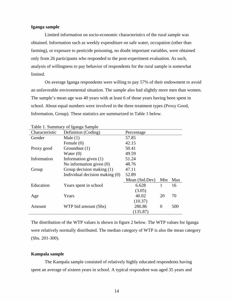
Iganga sample

Limited information on socio-economic characteristics of the rural sample was

obtained. Information such as weekly expenditure on safe water, occupation (other than

farming), or exposure to pesticide poisoning, no doubt important variables, were obtained

only from 26 participants who responded to the post-experiment evaluation. As such,

analysis of willingness to pay behavior of respondents for the rural sample is somewhat

limited.

On average Iganga respondents were willing to pay 57% of their endowment to avoid

an unfavorable environmental situation. The sample also had slightly more men than women.

The sample’s mean age was 40 years with at least 6 of those years having been spent in

school. About equal numbers were involved in the three treatment types (Proxy Good,

Information, Group). These statistics are summarized in Table 1 below.

Table 1. Summary of Iganga Sample Characteristic Definition (Coding) Percentage Gender Male (1) 57.85 Female (0) 42.15 Proxy good Groundnut (1) 50.41 Water (0) 49.59 Information Information given (1) 51.24 No information given (0) 48.76 Group Group decision making (1) 47.11 Individual decision making (0) 52.89 Mean (Std.Dev) Min Max Education Years spent in school 6.628

(3.05) 1 16

Age Years 40.02 (10.37)

20 70

Amount WTP bid amount (Shs) 286.86 (135.87)

0 500

The distribution of the WTP values is shown in figure 2 below. The WTP values for Iganga

were relatively normally distributed. The median category of WTP is also the mean category

(Shs. 201-300).

Kampala sample

The Kampala sample consisted of relatively highly educated respondents having

spent an average of sixteen years in school. A typical respondent was aged 35 years and

14

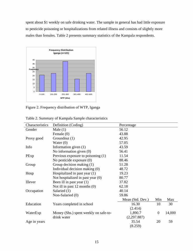
spent about $1 weekly on safe drinking water. The sample in general has had little exposure

to pesticide poisoning or hospitalizations from related illness and consists of slightly more

males than females. Table 2 presents summary statistics of the Kampala respondents.

Frequency Distribution Iganga (n=121)

0

5

10

15

20

25

30

35

40

0-100 101-200 201-300 301-400 401-500

WTP (Shs)

Frequency

Figure 2. Frequency distribution of WTP, Iganga

Table 2. Summary of Kampala Sample characteristics

Characteristics Definition (Coding) Percentage Gender Male (1)

Female (0) 56.12 43.88

Proxy good Groundnut (1) Water (0)

42.95 57.05

Info Information given (1) No information given (0)

43.59 56.41

PExp Previous exposure to poisoning (1) No pesticide exposure (0)

11.54 88.46

Group Group decision making (1) Individual decision making (0)

51.28 48.72

Hosp Hospitalized in past year (1) Not hospitalized in past year (0)

19.23 80.77

Illever Been ill in past year (1) Not ill in past 12 months (0)

37.82 62.18

Occupation Salaried (1) Non-Salaried (0)

40.14 59.86

Mean (Std. Dev.) Min Max Education Years completed in school 16.30

(2.414) 10 30

WaterExp Money (Shs.) spent weekly on safe-to-drink water

1,890.7 (2,297.887)

0 14,000

Age in years 35.54 (8.259)

20 59

15

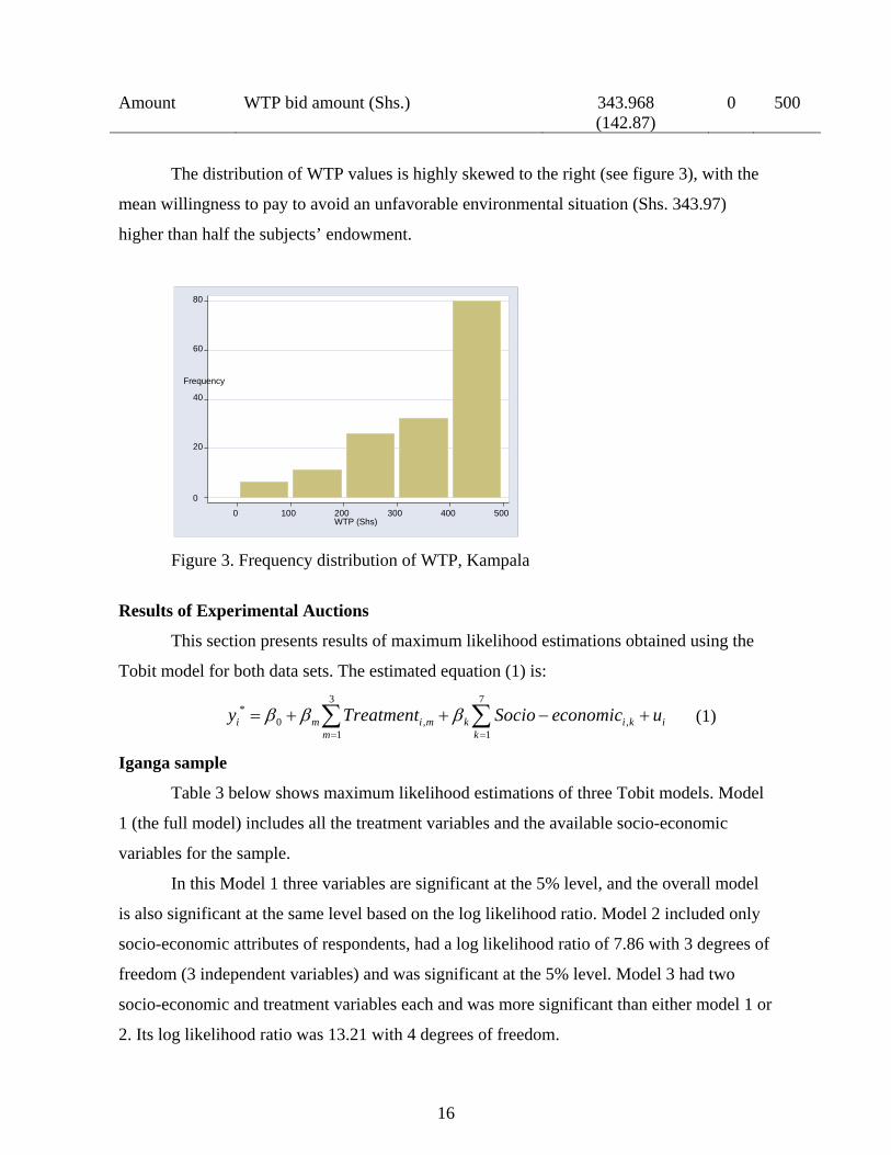
Amount WTP bid amount (Shs.) 343.968 (142.87)

0 500

The distribution of WTP values is highly skewed to the right (see figure 3), with the

mean willingness to pay to avoid an unfavorable environmental situation (Shs. 343.97)

higher than half the subjects’ endowment.

0

20

40

60

80

Frequency

0 100 200 300 400 500WTP (Shs)

Figure 3. Frequency distribution of WTP, Kampala

Results of Experimental Auctions

This section presents results of maximum likelihood estimations obtained using the

Tobit model for both data sets. The estimated equation (1) is: 3 7

*0 ,

1 1i m i m k i k

m ky Treatment Socio economic uβ β β

= =

= + + − +∑ ∑ , i (1)

Iganga sample

Table 3 below shows maximum likelihood estimations of three Tobit models. Model

1 (the full model) includes all the treatment variables and the available socio-economic

variables for the sample.

In this Model 1 three variables are significant at the 5% level, and the overall model

is also significant at the same level based on the log likelihood ratio. Model 2 included only

socio-economic attributes of respondents, had a log likelihood ratio of 7.86 with 3 degrees of

freedom (3 independent variables) and was significant at the 5% level. Model 3 had two

socio-economic and treatment variables each and was more significant than either model 1 or

2. Its log likelihood ratio was 13.21 with 4 degrees of freedom.

16

Gender, Education and the Group treatment variables had a significant effect on

Table 3. Maximum likelihood estimates of WTP - Iganga OLS Model 1 Model 2 Model 3 Coeff. Std.

Error Coeff. Std.

Error Coeff. Std.

Error Coeff. Std.

Error Age .0995 1.181 .3219 1.377 .278 1.406 - - Gender 48.283c 25.557 67.099b 29.485 74.245b 30.026 66.0094b 29.376 Educ -8.341b 4.1803 -10.406b 4.847 -9.866b 4.941 -10.041b 4.762 PGood 6.6099 24.937 10.488 28.792 - - - - Info -25.309 24.528 -27.7462 28.359 - - -26.761 27.958 Group -55.417b 24.900 -61.769b 28.711 - - -63.337b 28.234 Constant 345.969 58.016 351.293 67.186 307.479 63.039 367.833 41.192 R2 0.0988 - - - - - - Prob > F 0.0606 - - - - - - Log Likelihood - -672.476 -675.242 -672.569 LR 2χ (df) - 13.40(6) 7.86(3) 13.21(4)

Prob > chi2 - .0372 0.0489 0.0103 Pseudo-R2 - .0099 0.0058 0.0097 N 121 121 121 121

b significant at 5%, c Significant at 10%

bidding behavior of Iganga respondents. Males had higher WTP values than females. The

respondents with more formal education were willing to pay less to avoid bad environmental

outcomes. Subjects who were involved in Group treatments paid significantly less than those

involved in ‘self’ treatments. Information, good proxy and age were not helpful in predicting

WTP. Even after elimination of the Information treatment variable that was found not to

affect WTP, the gender, education and group variables continued to exert strong effect on

WTP (Model 3).

The signs of the coefficients were consistent across models. The Group, Info and

Educ. variables retained the same negative sign, while Gender and Age variables exerted

positive effects on WTP across all models. Also, like in the Kampala sample the OLS

estimates have the same directional effects on WTP as the ML estimates but are biased

downwards, and the variability in WTP explained by the variables (R2) in the OLS model is

low.

Kampala sample

The general-to-specific approach is adopted. Model 1 is the full model including all

hypothesized socio-economic and treatment variables. The model is significant at the 1%

17

level with a log likelihood of -600.359 (Table 4). The LR test for the null hypothesis that all

coefficients except the intercept are jointly zero is significant at the1% critical value level.

Using stepwise elimination of variables, an attempt was made to have a model with only

socio-economic variables. Model 2 retained three socio-economic variables and included one

treatment variable and is significant at the 10% level. Model (3) aimed to include all

treatment variables. However these all being binary limits the number of such variables that

can be included in the model. After dropping insignificant variables the final model retained

the Group treatment and two socio-economic variables and is significant at the 1% level.

All three models show that the grouping treatment variable (Group) was significant

in predicting WTP values. In addition, (at a lower significance level) previous exposure to

pesticide poisoning and weekly water expenditure had an effect on WTP. The other variables

and treatments did not show significant relationships with WTP values. All socio-economic

variables (except gender) were unable to predict bidding behavior.

Table 4. Maximum likelihood estimates of WTP – Kampala

OLS Model 1 Model 2 Model 3 Coeff. Std.

Error Coeff. Std. Error Coeff. Std.

Error Coeff. Std.

Error Age -1.4815 1.522 -1.827 1.977 -.3870 1.966 - - Gender 29.447 25.671 42.899 33.677 - - 47.460d 31.968 Educ .885 5.412 1.145 7.060 .6476 6.772 - - PGood -49.682c 27.868 -69.821c 36.757 - - - - Info -14.657 25.734 -25.494 33.599 - - - - Group -42.831d 26.674 -66.551c 35.346 -91.3303a 33.528 -100.738a 32.762 PExp 61.343d 38.232 93.393c 53.005 - - - - WaterExp .0091c .00544 .0147c .00743 .01036d .0074 .0108d .00737 Hosp -37.833 29.174 -52.012d 37.643 - - - - Salaried 78.326a 27.788 123.115a 37.267 - - - - Constant 360.574 104.99 387.706 137.276 399.1323 126.476 376.4491 34.575 R2 .1770 - - - - - - Prob >F .0133 - - - - - - Log L/hood - -600.3599 -656.8267 -671.054 LR 2χ (df) - 27.69 (10) 9.24 (4) 13.38 (3)

Prob > chi2 - 0.0020 0.0553 0.0039 Pseudo-R2 - .0225 .0070 0.0099 N 156 156 156 156

a Significant at 1%, c Significant at 10%, d Significant at 20%

The negative sign on the Group variable implies that subjects who participated in the

group treatment were more likely to have lower WTP values than those who participated in

‘self’ treatments. The (weak) positive sign on WaterExp and PExp variables suggests that

18

concern about exposure to pesticide poisoning influenced people to bid higher to avoid bad

environmental outcomes.

In Model 1 the expected WTP increases by Shs. 0.0146 when water expenditure

increases by Shs. 1, holding all other variables in the model constant. That is, the more a

person is willing to spend on safe drinking water, the more this person is willing to pay to

avoid a bad environmental situation. In addition, a salaried person’s expected WTP was Shs.

123.11 (24.6% of subject endowment) higher than a non-salaried person, all else being equal.

A general comment on the three models is necessary here. Important to note is the

consistency in signs on coefficients of variables across the models. The coefficient on Age

and Group variables is consistently negative and that on the Educ, WaterExp and Gender

variables is consistently positive. OLS estimates for the full model also presented in Table

4.6 have the same directional effect on WTP as maximum likelihood estimates. However, as

expected, they have a downward bias relative to the Maximum Likelihood Estimates.

Tests of Hypotheses

In this section the more parsimonious and/or significant models from the preceding

section are used to conduct simple hypothesis tests and to discuss these treatment effects. In

addition, the effects of two socio-economic variables (Gender, Education) are examined in

detail. The tcal value included in following hypothesis test tables is the calculated student’s t

statistic obtained as the ratio of the coefficient to its standard error and is compared with the

tabulated t-statistic ttab to determine the critical region for rejection of the null hypothesis. All

hypothesis tests are conducted at the 5% critical level of significance.

1. Does free-riding in health and environmental provision exist? Are there differences in

free-riding behavior between urban and rural populations?

0 3: 0H β = vs 1 3:H 0β <

where 3β is the coefficient on the Group variable. In both data sets (Table 5) , subjects bid

highest when involved in individual decision-making treatments. This is an indication of

free-riding behavior. Thus, even when individuals would presumably have preferred a

pesticide-free environment (proxied by the goods presented to them), they (individuals)

would rather have another person ‘paying’ for it.

19

Table 5. Test of Hypothesis One with Model 3

Kampala Iganga

3β -100.7382 -63.33695 Std. Error 32.76161 28.23376

calt 3.07488 2.24330

Is > calt tabt yes Yes Decision Reject 0H Reject 0H

2. Does providing information matter? How does content information influence bidding

behavior?

0 2: 0H β = vs 1 2:H 0β ≠

2β is the coefficient on the information treatment variable. In this case, a brief statement of

how pesticides in the air, food and water could affect humans and the environment was

provided to individuals in the ‘info’ treatment. Testing this hypothesis show that 2β was not

statistically significant in either of the three models in Iganga or Kampala data sets (Table 6).

Because of the direction on this coefficient, had the variable been significant, the sign would

have implied that providing information negatively influences WTP bids.

Table 6. Test of Hypothesis Two with Model 1

Kampala Iganga

2β -25.49357 -27.74552

Std. Error 33.59933 28.35918 calt 0.758752 0.97836

Is > calt tabt No No Decision Do not reject 0H Do not reject 0H

Results of hypothesis testing for information provision do not support rejecting the null

hypothesis. In these samples, information does not seem to influence bidding behavior.

3. How do gender differences influence bidding for health improvements. Are females more

sensitive to a better environment as it relates to their health than males?

0 4: 0H β = vs 0 4: 0H β <

20

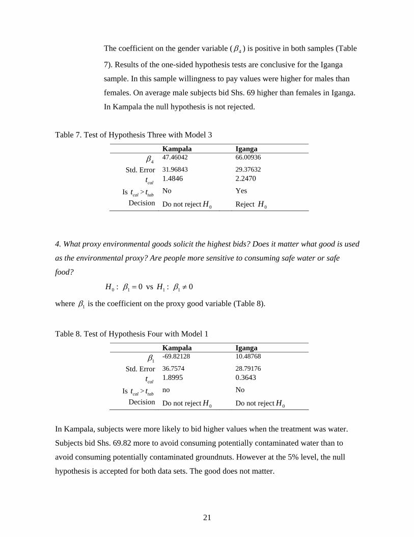
The coefficient on the gender variable ( 4β ) is positive in both samples (Table

7). Results of the one-sided hypothesis tests are conclusive for the Iganga

sample. In this sample willingness to pay values were higher for males than

females. On average male subjects bid Shs. 69 higher than females in Iganga.

In Kampala the null hypothesis is not rejected.

Table 7. Test of Hypothesis Three with Model 3

Kampala Iganga

4β 47.46042 66.00936

Std. Error 31.96843 29.37632

calt 1.4846 2.2470

Is > calt tabt No Yes Decision Do not reject 0H Reject 0H

4. What proxy environmental goods solicit the highest bids? Does it matter what good is used

as the environmental proxy? Are people more sensitive to consuming safe water or safe

food?

0 1: 0H β = vs 1 1:H 0β ≠

where 1β is the coefficient on the proxy good variable (Table 8).

Table 8. Test of Hypothesis Four with Model 1

Kampala Iganga

1β -69.82128 10.48768

Std. Error 36.7574 28.79176

calt 1.8995 0.3643

Is > calt tabt no No Decision Do not reject 0H Do not reject 0H

In Kampala, subjects were more likely to bid higher values when the treatment was water.

Subjects bid Shs. 69.82 more to avoid consuming potentially contaminated water than to

avoid consuming potentially contaminated groundnuts. However at the 5% level, the null

hypothesis is accepted for both data sets. The good does not matter.

21

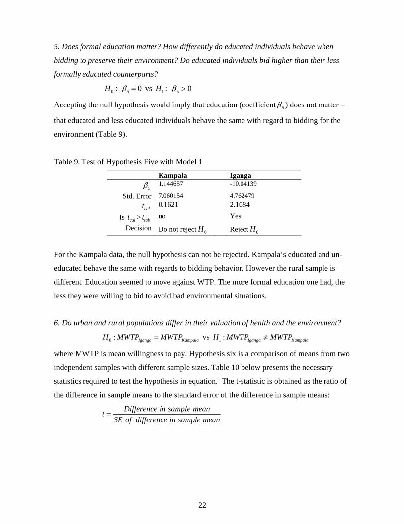
5. Does formal education matter? How differently do educated individuals behave when

bidding to preserve their environment? Do educated individuals bid higher than their less

formally educated counterparts?

0 5: 0H β = vs 1 5: 0H β >

Accepting the null hypothesis would imply that education (coefficient 5β ) does not matter –

that educated and less educated individuals behave the same with regard to bidding for the

environment (Table 9).

Table 9. Test of Hypothesis Five with Model 1

Kampala Iganga

5β 1.144657 -10.04139

Std. Error 7.060154 4.762479

calt 0.1621 2.1084

Is > calt tabt no Yes Decision Do not reject 0H Reject 0H

For the Kampala data, the null hypothesis can not be rejected. Kampala’s educated and un-

educated behave the same with regards to bidding behavior. However the rural sample is

different. Education seemed to move against WTP. The more formal education one had, the

less they were willing to bid to avoid bad environmental situations.

6. Do urban and rural populations differ in their valuation of health and the environment?

vs 0 : Iganga KampalaH MWTP MWTP= 1 : Iganga KampalaH MWTP MWTP≠

where MWTP is mean willingness to pay. Hypothesis six is a comparison of means from two

independent samples with different sample sizes. Table 10 below presents the necessary

statistics required to test the hypothesis in equation. The t-statistic is obtained as the ratio of

the difference in sample means to the standard error of the difference in sample means:

Difference in sample meant

SE of difference in sample mean=

22

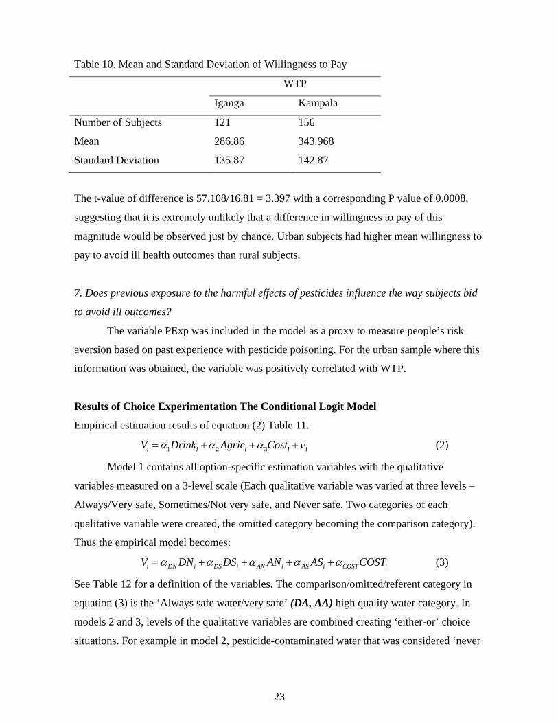
Table 10. Mean and Standard Deviation of Willingness to Pay

WTP

Iganga Kampala

Number of Subjects 121 156

Mean 286.86 343.968

Standard Deviation 135.87 142.87

The t-value of difference is 57.108/16.81 = 3.397 with a corresponding P value of 0.0008,

suggesting that it is extremely unlikely that a difference in willingness to pay of this

magnitude would be observed just by chance. Urban subjects had higher mean willingness to

pay to avoid ill health outcomes than rural subjects.

7. Does previous exposure to the harmful effects of pesticides influence the way subjects bid

to avoid ill outcomes?

The variable PExp was included in the model as a proxy to measure people’s risk

aversion based on past experience with pesticide poisoning. For the urban sample where this

information was obtained, the variable was positively correlated with WTP.

Results of Choice Experimentation The Conditional Logit Model

Empirical estimation results of equation (2) Table 11.

1 2 3i i iV Drink Agric Costi iα α α= + + ν+

iST

(2)

Model 1 contains all option-specific estimation variables with the qualitative

variables measured on a 3-level scale (Each qualitative variable was varied at three levels –

Always/Very safe, Sometimes/Not very safe, and Never safe. Two categories of each

qualitative variable were created, the omitted category becoming the comparison category).

Thus the empirical model becomes:

i DN i DS i AN i AS i COSTV DN DS AN AS COα α α α α= + + + + (3)

See Table 12 for a definition of the variables. The comparison/omitted/referent category in

equation (3) is the ‘Always safe water/very safe’ (DA, AA) high quality water category. In

models 2 and 3, levels of the qualitative variables are combined creating ‘either-or’ choice

situations. For example in model 2, pesticide-contaminated water that was considered ‘never

23

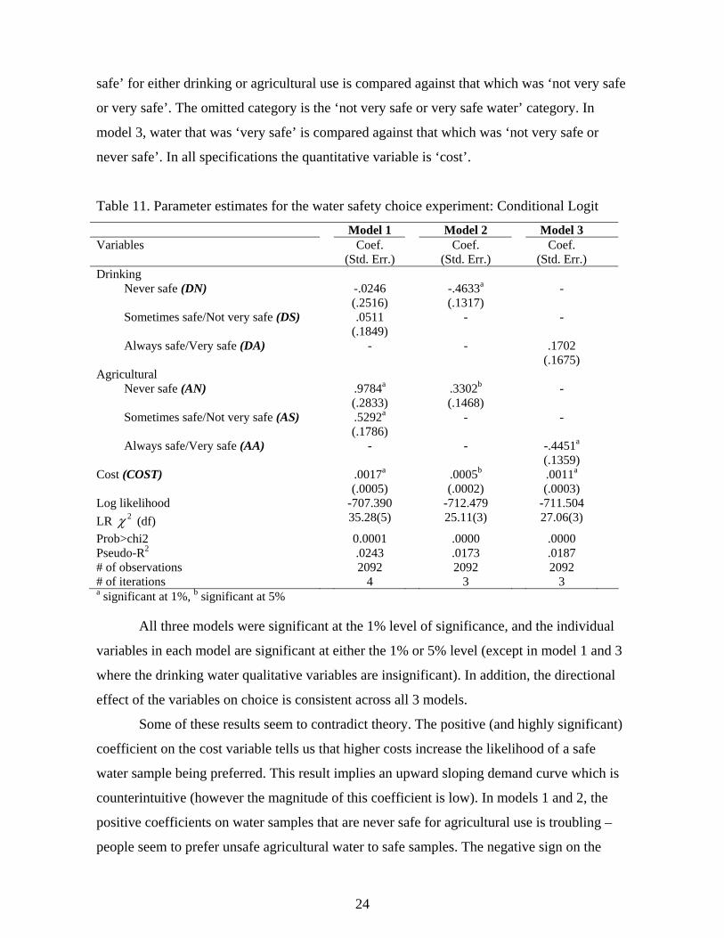
safe’ for either drinking or agricultural use is compared against that which was ‘not very safe

or very safe’. The omitted category is the ‘not very safe or very safe water’ category. In

model 3, water that was ‘very safe’ is compared against that which was ‘not very safe or

never safe’. In all specifications the quantitative variable is ‘cost’.

Table 11. Parameter estimates for the water safety choice experiment: Conditional Logit

Model 1 Model 2 Model 3 Variables

Coef. (Std. Err.)

Coef. (Std. Err.)

Coef. (Std. Err.)

Drinking Never safe (DN) -.0246

(.2516) -.4633a

(.1317) -

Sometimes safe/Not very safe (DS) .0511 (.1849)

- -

Always safe/Very safe (DA) - - .1702 (.1675)

Agricultural Never safe (AN) .9784a

(.2833) .3302b

(.1468) -

Sometimes safe/Not very safe (AS) .5292a (.1786)

- -

Always safe/Very safe (AA) - - -.4451a (.1359)

Cost (COST) .0017a (.0005)

.0005b

(.0002) .0011a

(.0003)

Log likelihood -707.390 -712.479 -711.504 LR 2χ (df) 35.28(5) 25.11(3) 27.06(3)

Prob>chi2 0.0001 .0000 .0000 Pseudo-R2 .0243 .0173 .0187 # of observations 2092 2092 2092 # of iterations 4 3 3 a significant at 1%, b significant at 5%

All three models were significant at the 1% level of significance, and the individual

variables in each model are significant at either the 1% or 5% level (except in model 1 and 3

where the drinking water qualitative variables are insignificant). In addition, the directional

effect of the variables on choice is consistent across all 3 models.

Some of these results seem to contradict theory. The positive (and highly significant)

coefficient on the cost variable tells us that higher costs increase the likelihood of a safe

water sample being preferred. This result implies an upward sloping demand curve which is

counterintuitive (however the magnitude of this coefficient is low). In models 1 and 2, the

positive coefficients on water samples that are never safe for agricultural use is troubling –

people seem to prefer unsafe agricultural water to safe samples. The negative sign on the

24

unsafe drinking water sample is intuitive – indicating people’s preference for water that is

either sometimes safe or always safe compared to that which is never safe for drinking.

Multiple Binary Logit Models

This section reports results from estimations of multiple binary logit models.

Understanding the differences in water attributes (safety levels/water quality levels and cost)

is key to understanding the trade-offs people made between the two water samples at each

choice occasion. With unlabeled experiments, such as this, analyzing the decisions of

respondents in these time periods requires considering each choice decision as a subset of a

multiple binary choice decision making setting. The operational model is equation (4):

1 2 3 4i iq iq iqV Group Educ Gender Ageiqβ β β β= + + + +

5 6 7iq iq iqSalary PExp illeverβ β β+ + (4)

Description of Choice Occasions (t = 1, …, 8)

Each respondent made a choice decision at each choice occasion. In choice occasion

1, water samples A and B were differentiated only in terms of the agricultural water quality

and cost. Subject’s choice of option A over option B was an indication of their preference for

free, low quality (unsafe) agricultural water over not-very safe (medium quality) water at a

cost of Shs. 300.

In choice occasion 2 (and 3), choice of option A is a preference for unsafe

agricultural water at a cost of Shs.100 (and medium safety/medium quality, free agricultural

water) over safe agricultural water at a cost of Shs. 500. Choice of option A in choice

occasion 4 (and 7) is a preference for unsafe water samples at Shs. 200 over unsafe drinking

water at Shs. 300 (and not very safe drinking water at Shs. 500). In choice occasion 5 (and 6)

choice of option A is a preference between safe water samples at Shs. 300 (Shs. 500) over

not very safe drinking water (never safe drinking water). In choice occasion 8 choice of

option A implied preference for safe agricultural water (at a medium cost of Shs. 200)

compared to free medium quality (medium safety) agricultural water.

25

26

Coefficient Estimates

The same approach is employed to obtain the multiple logit estimates as was

employed in the conditional logit model. Stepwise elimination of insignificant variables is

performed. That is, model 1 (in Table 12 a, b) below contains all individual-specific

variables. After elimination of insignificant variables from Model 1, Model 2 is obtained.

It is important to note the general consistency in signs of the coefficients in the full

and restricted models (models 1 and 2) of each choice occasion. In addition the significant

variables in the full models retain their effect in the restricted models. A general comment

can be made that the significance of individual variables in the choice data is low. Models for

choice occasion 1, 2, 4 and 8 have individual significant variables at the 5% level.

The dependent variable in all these models is the respondent’s binary choice of a

water sample of given attributes (explained in the preceding section). The following

discussion pertains to the more parsimonious model in each choice occasion. In choice

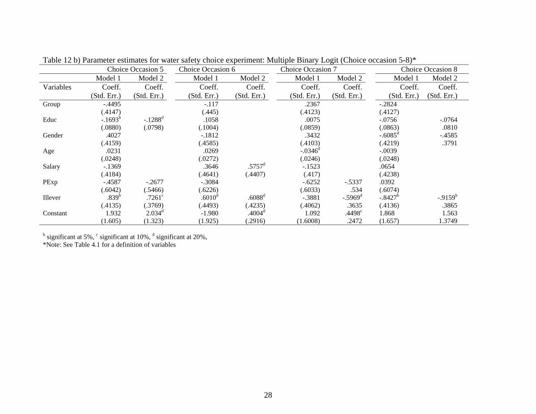
occasion 1 the variable PExp had an effect on preference of a water sample. This result is

consistent with risk averse behavior. Respondents who had been previously exposed to

pesticide poisoning were more likely to prefer a safer water sample (at a cost) in option B

than a free but unsafe water sample in option A. The other individual-specific variables were

not important predictors of choice of a water sample.

In choice occasion 2 the gender variable was significant and negative indicating that

males were more likely to prefer a more expensive water sample with high agricultural

quality than an unsafe sample at Shs.100. This result is consistent with the experimental

auction results which depicted males as having higher willingness to pay than females in

general. In choice occasion 4 only the education (Educ) variable was significant at the 5%

level. The more education one had, the less likely they preferred option A (with medium

safety levels for both agricultural and drinking water, at a cost of Shs 200) over option B

(safe agricultural water at a cost of Shs. 500). The negative coefficient on the ‘illever’

variable in choice occasion 8 suggests that respondents who had had an episode of illness in

the past year were more inclined to prefer option B (safe agricultural water at a cost of 200)

than option A (free medium quality agricultural water). This result runs counter to

expectations. Experience with past illnesses is expected to induce risk averse behavior such

Table 12 a) Parameter estimates for water safety choice experiment: Multiple Binary Logit (Choice occasion 1-4)* Choice Occasion 1 Choice Occasion 2 Choice Occasion 3 Choice Occasion 4 Model 1 Model 2 Model 1 Model 2 Model 1 Model 2 Model 1 Model 2Variables Coeff.

(Std. Err.) Coeff.

(Std. Err.) Coeff.

(Std. Err.) Coeff.

(Std. Err.) Coeff.

(Std. Err.) Coeff.

(Std. Err.) Coeff.

(Std. Err.) Coeff.

(Std. Err.) Group -.6612d

(.4153) -.6992c .3864

.0725 (.4142)

-.1189 (.4105)

-.2699 (.4114)

Educ -.0823 (.0859)

-.1316d .0829

.0242 (.0856)

-.0340 (.0855)

-.221b (.1003)

-.2336b (.0951)

Gender .4008 (.4111)

.4193

.3889 -.9324b

(.4244) -.8849b (.4107)

.3531 (.4139)

.3396 .(3962)

-.5725d (.4189)

-.2619 (.3707)

Age -.0077 (.0248)

.0147 (.0249)

-.0048 (.0245)

-.0111 (.0252)

Salary -.3254 (.4141)

-.7644c (.4273)

-.656d (.4069)

-.2745 (.4185)

-.3726 (.4041)

-.495 (.4189)

PExp -1.958a (.72498)

-1.796a .6517

-.7348 (.6178)

-.813d (.6020)

-.1565 (.5978)

.1506 (.6092)

Illever -.0068 (.4058)

-.4595 (.4113)

-.0208 (.4068)

.2277 (.4090)

Constant 2.102d (1.628)

2.547c 1.448

.3234 (1.575)

1.051a (.3760)

.2657 (1.607)

-.5348d (.3561)

4.753b (1.902)

4.1019a (1.58)

a significant at 1%, b significant at 5%, c significant at 10%, d significant at 20% *Note: See Table 2 for a definition of variables

27

28

Table 12 b) Parameter estimates for water safety choice experiment: Multiple Binary Logit (Choice occasion 5-8)* Choice Occasion 5 Choice Occasion 6 Choice Occasion 7 Choice Occasion 8 Model 1 Model 2 Model 1 Model 2 Model 1 Model 2 Model 1 Model 2Variables Coeff.

(Std. Err.) Coeff.

(Std. Err.) Coeff.

(Std. Err.)Coeff.

(Std. Err.)Coeff.

(Std. Err.) Coeff.

(Std. Err.)Coeff.

(Std. Err.) Coeff.

(Std. Err.)Group -.4495

(.4147) -.117

(.445) .2367

(.4123) -.2824

(.4127)

Educ -.1693b (.0880)

-.1288d (.0798)

.1058 (.1004)

.0075 (.0859)

-.0756 (.0863)

-.0764 .0810

Gender .4027 (.4159)

-.1812 (.4585)

.3432 (.4103)

-.6085d (.4219)

-.4585 .3791

Age .0231 (.0248)

.0269 (.0272)

-.0346d (.0246)

-.0039 (.0248)

Salary -.1369 (.4184)

.3646 (.4641)

.5757d (.4407)

-.1523 (.417)

.0654 (.4238)

PExp -.4587 (.6042)

-.2677 (.5466)

-.3084 (.6226)

-.6252 (.6033)

-.5337 .534

.0392 (.6074)

Illever .839b (.4135)

.7261c (.3769)

.6010d (.4493)

.6088d (.4235)

-.3881 (.4062)

-.5969d .3635

-.8427b (.4136)

-.9159b .3865

Constant 1.932 (1.605)

2.034d (1.323)

-1.980 (1.925)

.4004d (.2916)

1.092 (1.6008)

.4498c .2472

1.868 (1.657)

1.563 1.3749

b significant at 5%, c significant at 10%, d significant at 20%, *Note: See Table 4.1 for a definition of variables

that subjects would want to avoid further exposure by preferring the safer water sample, even

for agricultural use.

Discussion of Choice Experimental Models

It is apparent that the conditional and logit models were not properly suited to this data,

perhaps due to specification bias. Goodness of fit measures indicated that not much variation

in the observed behavior was predicted by the attributes in the models. All models converged

after a few iterations – an indication of little improvement between the model

with, and one without the predictors.14 Although interpretation of the pseudo R2 statistic in

maximum likelihood is different from that in OLS, the goodness-of fit measure for these

three models seems rather low. Logit models with extremely good fit have pseudo R2 in the

0.2-0.4 range. The range in these models was 0.017 – 0.024.

Conclusions

Among the strong results from this study was the manifestation of free riding in

public goods provision, differences in rural and urban sample bidding behavior, and

differences in bidding behavior due to income differences. The first of these suggests

government intervention may be necessary if one is to see improvement in both health and

environmental provision. If the problems associated with pesticides in the environment and

their probable effects on humans are to be addressed, reliance on the individuals directly

concerned will not be sufficient and a concerted effort of a ‘third party’ may be necessary – a

typical public goods problem.

Differences in willingness to pay values between urban and rural populations suggest

that programs should be tailored to suit different locations. Rural populations are less willing

to pay to avoid ill-health outcomes and also, since their line of work exposes them more to

pesticides than the urban population, are more prone to potential contamination. Perhaps the

rural population feels that it is their obligation to be provided with a clean environment, or

14 Maximum likelihood, an iterative process, starts out with an approximated starting value of what the logit coefficients should be and determines the direction and size of the change in logit coefficients which will increase the log likelihood, and the process continues until there are very small improvements in the log likelihood.

29

they generally do not care as much about their health and environment, or they perceive the

concentration levels in the pesticides to be too low as to cause them any damage, or indeed as

one rural respondent mentioned: “I have been subjected to these chemicals for a long time.

But look at me, I am still healthy”. Such reasoning, if widespread in the rural population, is

an indication that rural people may be discounting the future heavily, that to them, what

matters is their immediate survival. In any case the rural-urban differences in WTP suggest

that any health and environment improvement programs may require different interventions

for the different regions.

Perhaps the most important explanation for differences in bidding behavior for health

and environmental improvement can best be attributed to differences in income, rather than

differences in non-economic issues (recall that information treatments and education had no

significant positive effect on willingness to pay). The high willingness to pay to avoid

contamination that higher income (salaried and urban) subjects had is an indication that

increased incomes induce health and environmental awareness. As economic development

increases and people’s incomes increase, the demand for environmental quality by Ugandans

can be expected to rise. People may devote some of their increased income to improving

their health and their environment, and protection of natural resources.

Inference made from results from both choice experiments and experimental auctions

varied. Knowledge of this variation is important when attempting to compare or combine

results from the two methods. One practice that is currently on the increase is to combine

revealed preference and stated preference results to predict behavior. When results from

either set of data are either inaccurate or doubtful, the combination becomes inappropriate. In

the current study, even with the same individuals, and when the ‘goods’ being valued were

identical, different methods yielded diverging results, suggesting that they should not be

combined.

In the strictest sense that choice experiments valued environmental improvements and

experimental auctions valued health improvements, the failure to obtain choice experimental

data from rural respondents precludes the testing of whether urban populations care more

about their environment than the rural populations. However differences existed between

salaried and non-salaried respondents and with the positive correlation this variable has with

incomes, results from the experimental auctions can be interpreted as higher income

populations care more about a cleaner environment than low income populations.

30

There may not be as clear a distinction between “health and the environment” as

presented in this study. There shouldn’t be. The two components are inter-related. One needs

a good environment to support human health, and some life-support activities of humans may

be put at risk when the environment is overly degraded. Environmental valuation requires

creating a link between changes in the environment and how they affect health, and then

estimating how these changes in health are reflected in WTP values.

31

References

Berger, M.C., G.C. Blomquist, D. Kenkel, and G.S. Tolley. 1987. “Valuing changes in Health risks: A comparison of alternative measures.” Southern Economic Journal. 53(4):967-984. Bonabana-Wabbi, J. 2008. Ph.D. Dissertation, Department of Agricultural and Applied Economics, Virginia Tech. Boxall, P.C., W.L. Adamowicz, J. Swait, M.Williams, and J. Louviere. 1996. “A Comparison of Stated Preference Methods for Environmental Valuation.” Ecological Economics. 18:243-253. Brethour, C., and A. Weersink. 2001. “An economic evaluation of the environmental benefits from pesticide reduction.” Agricultural Economics 25:219-226. CRSP, Collaborative Research Support Program. 2002. Annual Report. http://www.oired.vt.edu/ipmcrsp. Internet accessed. Cuyno, L.C., G.W. Norton., and A. Rola. 2001. "Economic analysis of environmental benefits of integrated pest management: A Philippine case study." Agricultural Economics 25:227-233. DeShazo, J.R., and G. Fermo. 2002. “Designing Choice Sets for Stated Preference Methods: The Effects of Complexity on Choice Consistency.” Journal of Environmental Economics and Management 44(1):123-143. Ecaat, J. 2004. A Review of the Application of Environmental Impact Assessment (EIA) in Uganda. A Report Prepared for the United Nations Economic Commission for Africa. Food and Agricultural Organization. 2004. “FAO warns of the Dangerous Legacy of Obsolete Pesticides”. Press Release 99/31. http://www.fao.org/WAICENT/OIS/PRESS_NE/PRESSENG/1999/pren9931.htm. Internet Accessed June 2004. Freeman, A. M. 2003. The measurement of environmental and natural resource values: Theory and Methods. 2nd edition. Washington DC. Resources for the Future. 1616 P Street, NW, Washington, DC. Hanley, N., R.E. Wright, and V. Adamowicz. 1998. “Using choice experiments to value the environment. Design issues, current experience and future prospects.” Kluwer Academic Publishers. Printed in the Netherlands. Environmental and Resource economics 11(3-4): 413-428. Hanley, N., J. Grande, B. Álvarez-Farizo, C. Salt, and M. Wilson. 2001. Risk perceptions, risk-reducing behavior and willingness to pay: radioactive contamination in food following a nuclear accident. Working papers. Department of Economics. University of Glasgow. Higley, L.G., and W.K. Wintersteen. 1992. “A novel approach to environmental assessment of pesticides as a basis for incorporating environmental costs into EILs”. American Entomologist 38:34-39. Huck, S. 2007. Experimental methodology: Oligopoly experiments. Experimental Economics. University College London. www.ucl.ac.uk/~uctpshu/phdmicro_2.pdf Jeyaratnam, J. 1990. “Acute Pesticide Poisoning: A Major Global Health Problem.”

32

World Health Statistics Quarterly 43:139-144. Kegley, S., B. Hill, and S. Orme. 2007. PAN Pesticide Database, Pesticide Action Network, North America. http:www.pesticideinfo.org. Pesticide Action Network, North America. Kishimba, M.A., L. Henry, H. Mwevura, A.J. Mmoshi, M. Mihale, and H. Haller. 2004. “The status of pesticide pollution in Tanzania.” Talanta 64: 48-53. Kovach, J., C. Petzoldt, J. Degni and J. Tette. 1992. “A method to measure the environmental impact of pesticides.” New York’s Food and Life Science Bulletin. 139:1-8. Louviere, J., D. Hensher, and J. Swait. 2000. Stated Choice Methods. Analysis and Application. Cambridge: Cambridge University Press. Lusk, J.L., and T.C. Schroeder. 2004. “Are Choice Experiments Incentive Compatible? A test with quality Differentiated Beef Steaks.” American Journal of Agricultural Economics. 86(2):467-482. Maupin, J.D. 2006. Valuing the Environmental Benefits from GM Products Using an Experimental Procedure: Lessons from the United States and the Philippines. Master’s thesis. Department of Agricultural and Applied Economics. Virginia Tech. Mullen, J.D., G.W. Norton, and D.W. Reaves. 1997. “Economic Analysis of environmental benefits of integrated pest management.” Journal of Agricultural and Applied Economics. 29 (2): 243-253. Ngowi, A.V. 2002. Health Impact of Exposure to Pesticides in Agriculture in Tanzania. Unpublished Phd. Dissertation. University of Tampere. Tampere School of Public Health, Finland. Reiff, L.O., and A.L. Barbosa. 2005. “Housing Stock in Brazil: Estimation based on a Hedonic Price Model.” Bank for International Settlements (BIS) Papers. bis.org. No. 21. Internet accessed, October 2007. Ryan, M., A. Bate, C.J. Eastmond, and A. Ludbrook. 2001. “Use of discrete choice experiments to elicit preferences.” Quality in Health Care 10(Suppl I):i55-i60. Smith, V.L. 1976. Experimental Economics: Induced Value Theory. The American Economic Review. Papers and Proceedings of the Eighty-eighth Annual Meeting of the American Economic Association. 66(2) 274-279. The Daily Monitor, 2007. DDT: Survival weapon or threat? http://www.monitor.co.ug The New Vision, 2007. “Uganda clings on to DDT for malaria” http://www.newvision.co.ug/D/8/459/455871/ Uganda, The Republic of. 2007. Ministry of Agriculture, Animal Industry and Fisheries. Summary of the National Agricultural Statistics 2005-2006. http://www.agriculture.go.ug/statistics.htm Zwerina, K., J. Huber, and W.F. Kuhfeld. 2007. A general method for constructing efficient choice designs. http://support.sas.com/techsup/technote internet accessed, 2007.

33