he idem ann a
TRANSCRIPT

8/2/2019 He Idem Ann A
http://slidepdf.com/reader/full/he-idem-ann-a 1/10
Effects of Detail in Wireless Network Simulation
John Heidemann, Nirupama Bulusu, Jeremy Elson,Chalermek Intanagonwiwat, Kun-chan Lan, Ya Xu,
Wei Ye, Deborah Estrin, Ramesh Govindan
USC/Information Sciences Institute
To appear, SCS Communication Networks and
Distributed Systems Modeling and Simulation Conference, January 2001
USC/ISI TR-2000-523b
AbstractExperience with wired networks has provides guidance about
what level of detail is appropriate for simulation-based proto-
col studies. Wireless simulations raise many new questions
about appropriate levels of detail in simulation models for
radio propagation and energy consumption. This paper de-
scribes the trade-offs associated with adding detail to simula-
tion models. We evaluate theeffects of detail in five case stud-
ies of wireless simulations for protocol design. Ultimately
the researcher must judge what level of detail is required for
a given question, but we suggest two approaches to cope with
varying levels of detail. When error is not correlated, net-
working algorithms that are robust to a range of errors areoften stressed in similar ways by random error as by detailed
models. We also suggest visualization techniques that can
help pinpoint incorrect details and manage detail overload.
Keywords: wireless network simulation; simulation val-
idation, detail, accuracy; energy-aware ad hoc routing; data
diffusion; localization; robotics; network protocol visualiza-
tion
1 INTRODUCTION
Selecting thecorrect levelof detail (or levelof abstraction) fora simulation is a difficult problem. Too little detail can pro-
duce simulations that are misleading or incorrect, but adding
detail requires time to implement, debug, and later change, it
¡
This research is supported by the Defense Advanced Research Projects
Agency (DARPA) through the VINT project under DARPA contract ABT63-
96-C-0054, the SCADDS project under DARPA contract DABT63-99-1-
0011, and the SCOWR project through NSF grant ANI-9979457.
For questions concerning this paper, please contact the authors in care
of John Heidemann, [email protected].
slows down simulation, and it can distract from the researchproblem at hand. Designing simulations to study a protocol
inherently involves making choices in which protocol details
to implement or use.
Although a number of network simulation packages are
available, they do not remove this burden from the designer.
In custom simulators, researchers typically include only the
minimum possible details outside the immediate area of
study. Existing simulators (such as Opnet, ns-2 [5], Par-
sec [2], and SSF [8]) provide detailed protocol implementa-
tions, but what level of detail is required in new protocols, or
in adapting existing protocols to model new hardware? Some
simulators ease the cost of changing abstraction with multi-
ple, selectable levels of detail (for example, ns [17]), but the
design choice must still be made.
Choices about detail are particularly difficult for wireless
network simulations. Wide experience with the important
components of wired networks over the last 30 years allows
significant abstraction. For example, point-to-point links are
often represented as a simply by bandwidth and delay with
a queue; framing, coding, and transmission errors are sim-
ply ignored or mathematically modeled. The younger field
of wireless networking provides less guidance on what ab-
stractions are appropriate. Low-level details can have a large
effect on performance, but detailed simulations can be very
expensive (for example, radio propagation).This paper explores the question of what level of detail
is needed for simulations of network protocols in wireless
domains. We begin by looking at the trade-offs in differ-
ent levels of detail in simulations. We then consider five
case studies: energy consumption in ad hoc routing, data
diffusion, radio-based outdoor localization, communications-
driven robot following algorithms, and visualization of wire-
less simulations. The contribution of this paper is two-fold:
first, by examining the effects of details on wireless simu-
1

8/2/2019 He Idem Ann A
http://slidepdf.com/reader/full/he-idem-ann-a 2/10
lations we help the networking simulation community judge
the relevance of simulation studies. Second, we identify two
different ways simulation results can be spoiled by too little
detail, and two cases where fairly abstract simulations suc-
cessfully model real-world behavior.
2 TRADE-OFFS OF DETAIL IN
WIRELESS SIMULATION
We next consider the trade-offs of more detailed or abstract
simulations.
A common goal is to infuse the simulation with as much
detail as possible to provide a “realistic” simulation. This
approach is attractive: a fully realistic simulation ought to be
able to reproduce the results of laboratory experiments or net-
work use by end-users. Failing to implement details guaran-
tees that they won’t be reflected in a simulation; for examplea wireless propagation model that doesn’t consider concur-
rent transmissions will not model the hidden terminal effect.
Furthermore, details at multiple protocol levels can reveal im-
portant interactions between layers. For example, router syn-
chronization was first studied in simulation [14].
Yet a “fully realistic” simulation is not possible—does one
stop at the network layer? they physical layer? electrons or
photons? Simulation designers must limit the level of detail
somewhere. The challenge is to identify what level of de-
tail does not affect answers to the design questions at hand.
For example, we know of no network simulator that consid-
ers details of a CPU’s instruction set or memory hierarchy—
these do not affect design questions relevant to wireless simu-
lations. Yet these details are critical to other networking prob-
lems such as very rapid routing [11].
There are several reasons to avoid excessive detail. Sim-
ulation run-time is adversely affected by detail. Implemen-
tation and debugging time is increased, and undetected bugs
in distant layers can produce inaccuracies. Even if debugged,
protocol details change over time. For example, an extremely
detailed implementation of WaveLAN from a few years ago
would today be superseded by the 802.11 standard today.
Sometimes getting all the details may be impossible, if they
are left open (or implementation-dependent) in the specifica-
tion, or when trying to predict future behavior with protocolsnot yet implemented or standardized. Finally, for many of
these reasons simulations often mix levels of detail in differ-
ent components. A very detailed, microsecond-level MAC
simulation may be forced to use a more abstract propaga-
tion model (because all objects in the terrain were not spec-
ified) and an older TCP implementation (perhaps not includ-
ing SACK or recently standardized extensions). Simulations
with detailed hardware models may have abstract (perhaps
randomized) scenarios of node placement, transmission, and
movement.
There are several reasons for intentionally choosing a high
level of abstraction for simulation. Distillation of a research
question to its essence can provide insight not colored by ar-
bitrary details of specific proposed solutions. For example,
although multiple resource reservation and quality-of-service
protocols have been proposed, Breslau and Shenker use a
very abstract service model to focus on the central issue of
the benefits of reservations [6]. When exploring a new area
where many issues are unclear, the need to quickly explore a
variety of alternatives can be more important than a detailed
result for a specific scenario. For this kind of nimble sim-
ulation, relative comparisons of alternatives are often more
important than a single detailed quantitative result. A more
abstract simulation can also make the effects of a change in
algorithm distinct, where they would be obscured by other
effects in a more detailed simulation. Finally, omission of
simulation detail can improve performance by multiple or-ders of magnitude [17]. Memory and run-time improvements
due can offer results sooner, or allow larger or longer exper-
iments, revealing different aspects of protocol behavior. For
example, the relative performance of ad hoc routing protocols
differs with large numbers of nodes [10].
The primary risk of simulation abstraction is the unknown.
Would additional detail change the conclusions of the simu-
lation study? This problem is particularly challenging when
entering a relatively unexplored area where researcher’s in-
tuitions may be underdeveloped. Validation of simulations
against more detailed simulations and experimental measure-
ments can answer this question. But the cost of validation
is fairly high: careful experiments require implementing thedetails in question or purchasing sufficient hardware for real-
world experiments.
Over time, the results of validation experiments will allow
the community to build an understanding of what details are
important. The community has begun sharing this informa-
tion through workshops such as the DARPA/NIST Network
Simulation Validation Workshop [9]. We next consider sev-
eral case studies that have arisen in our research as further
examples.
Table 1 summarizes the cases we examine, the relevant de-
tails that were considered, and how those details affected the
results of the simulation study. We found that choice of de-tail had several different results on the studies. Lack of detail
caused wrong answers in two ways, either because they were
simply incorrect , wrong or actively misleading, or because
they were inapplicable: technically correct but providing an
answer to part of the design space that may not be sensible
or relevant. In two other cases, relatively abstract approaches
were found to produce correct results, either because the ap-
plication was insensitive to the details at hand, the outputs
of the application had an existing component of noise that
2
8/2/2019 He Idem Ann A
http://slidepdf.com/reader/full/he-idem-ann-a 3/10
Case Relevant detail Effects
energy-conscious ad-hoc routing ( ¢ 3) energy consumption model (idle behavior) incorrect results
data diffusion ( ¢ 3) MAC protocol inapplicable results
localization ( ¢ 4.1) radio propagation model correct results, application insensitive to detail
robot following ( ¢ 4.2) radio propagation model correct results, application robust to error
protocol visualization ( ¢ 5) packet visualization strategy utility of visualization
Table 1: Case studies examined in this paper and how detail affected study results.
swamped any variation additional details provide, or because
the application was robust to details, the algorithm was self-
correcting to errors. Finally, for the case of visualization we
found the approaches to handling detail simply affect the use-
fulness of the visualization.
3 ENERGY CONSUMPTION IN AD
HOC ROUTING
Our first case study considers energy consumption when
routing data in ad hoc networks. We examine two recent
studies in this area: an evaluation of data diffusion [18], and
a study of an energy-saving variations of on-demand ad hoc
routing protocols [24]. Choice of appropriate models of ra-
dio energy consumption and MAC protocols make can com-
pletely change the conclusions of these studies.
Several models of energy consumption for wireless com-
munication have been used in literature:£
Successfully sent or received packets incur an energy
cost.
£
MAC-level costs can be considered—MAC-level re-transmissions, CTS/RTS, and packets that are unsuc-
cessfully sent or received incur a cost.
£
Energy consumed while listening (or “idle”, having the
radio powered on but not actively sending or receiving)
can also be modeled.
£
Non-radio system costs can be considered (display,
CPU, disk drive).
£ Battery internals (non-linearity, temperature sensitivity,
battery memory, etc.) can be considered.
Selecting the right level of detail depends on the research
question being considered. For most research questions about
networking protocols, non-radio components (for example,
the display) can be factored out as a fixed overhead, although
in some cases CPU-intensive work must be considered (for
example, software radios [4], or MPEG playout). Similarly,
for rough comparisons of protocols, detailed battery models
are not required—a reasonable simplifying assumption is that
memory or temperature will affect all protocols equally.
ad hoc routing protocol
e n e r g y c o n s u m e d ( J )
AODV DSR DSDV TORA
0
10
20
30
w / o u t i d l e e n e r g y c o n s u m p t i o n
w i t h i
d l e e n e r g y c o n s u m p t i o n
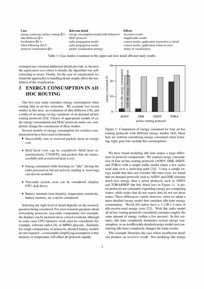
Figure 1: Comparison of energy consumed for four ad hoc
routing protocols with different energy models (left, black
bars are without considering energy consumed when listen-
ing; right, gray bars include this consumption).
We have found modeling idle time makes a large differ-
ence in protocol comparisons. We studied energy consump-
tion of four ad hoc routing protocols (AODV, DSR, DSDV,
and TORA) with a simple traffic model where a few nodes
send data over a multi-hop path [24]. Using a simple en-
ergy model that does not consider idle-time costs, we found
that on-demand protocols such as AODV and DSR consume
much less energy than a priori protocols such as DSDV
and TORA/IMEP (the left, black bars in Figure 1). A pri-
ori protocols are constantly expending energy pre-computing
routes, while nodes that do not source data do not use these
routes. These differences vanish, however, when we adopt a
more detailed energy model that considers idle-time energy
consumption. WaveLAN radios have a 1:1.05:1.4 ratio of
idle:receive:send energy costs [23]. With this radio model
all ad hoc routing protocols considered consume roughly the
same amount of energy (within a few percent). In this sce-
nario, idle time completely dominates system energy con-
sumption, so an insufficiently detailed energy model (not con-
sidering idle time) completely changes the study results.
This example illustrates the case where insufficient detail
can produce an incorrect result. Not modeling idle energy
3
8/2/2019 He Idem Ann A
http://slidepdf.com/reader/full/he-idem-ann-a 4/10
consumption indicates minimal differences between ad hoc
routing protocols, while adding idle energy shows clear dif-
ferences. Future wireless networking researchers should in-
clude these details in their power models and should use care
when interpreting prior published results that use overly sim-
plified models.Choice of MAC protocol is also closely tied with radio en-
ergy consumption. We have studied data diffusion protocols,
evaluating the power consumption of data diffusion as com-
pared to simple flooding and an idealized multicast [18]. The
goal of these experiments was to provide energy-conserving
protocols for long-lived sensor networks. Again we had trou-
ble with inappropriate models of radio energy consumption;
all protocols behaved similarly when idle costs were consid-
ered. In this case, the problem was an inappropriate MAC
protocol.
Figure 2 shows the comparison of data diffusion and two
alternatives, with a TDMA-like energy model (Figure 2(a))
and an 802.11 energy model (Figure 2(b)). (Because at this
time we did not have a TDMA model in our simulator, we
approximated it by adjusting the energy model. We plan to
redo these experiments with different model MAC models.)
As shown in the figure, choice of the MAC layer produces
very different conclusions when comparing the algorithms,
Figure 2(b) suggests there is no significant difference, while
Figure 2(a) shows a noticeable difference.
In this case, the conclusion is somewhat more subtle. Re-
sults of simulations with 802.11 protocols are not technically
wrong, but they are inappropriate . While one could use an
802.11 MAC for these applications, that would be poor de-
sign choice since long-lived sensor networks need an energy-conserving MAC like TDMA. Because the details are inap-
propriate, they result in conclusions (the algorithms are all
equivalent) that are incorrect for a well-designed system.
These examples suggest that idle-time and MAC protocols
are important details for wireless communication studies with
PC-like network nodes. We have not seen evidence that fur-
ther details (power consumption of other system components
or models of battery internals) alter research results in this
domain. Additional experience is needed to validate this as-
sumption. These assumptions may not hold for studies of
increasingly tiny (dust-mote-sized) nodes [21]. We hypothe-
size that as node and radio power consumption shrinks, and
as node lifetime increases, additional details will become im-portant.
4 RADIO PROPAGATION MODELS
Our next two studies consider the problems of radio-based lo-
calization (determining a node’s location) and robot follow-
ing. In both cases, we found the level of detail of the radio
propagation model important.
Even more than energy models, many levels of detail are
employed in radio propagation models with a single sender
and receiver:
£
The simplest models consider only propagation distance
from sender to receiver with a fixed formula for signalloss.
£ Slightly more detailed models might use different mod-
els for near and far receivers (for example, the Friis and
two-ray ground reflection approximations).
£ A statistical approximation of shadowing might be
added.
£
A more detailed model might consider signal attenu-
ation from large obstacles, perhaps modeling line-of-
sight communication differently from indirect commu-
nication.
£
Very detailed models would consider antenna geome-
tries (orientation, distance off ground) and perform de-
tailed radio ray-tracing to estimate reflection.
In addition, models may or may not take in the relative power
of interfering transmissions.
Radio propagation varies greatly, especially indoors, mo-
tiving very detailed propagation models. Unfortunately, ac-
curate models become very computationally expensive and
require much more detail about the environment than is typi-
cally available.
An attractive alternative is to couple a simple model with
some level of statistical loss, but there has been limited ex-
perience with how less detailed models change network be-
havior. We have evaluated this question in two case studies,
one where a very simple model proved surprisingly effective
in a restricted domain, and then a robotics-inspired approach
to designing software to be robust to model error.
4.1 Radio-based outdoor localization
Sometimes simple radio propagation models can be quite ef-
fective for the purposes of a problem. We are exploring the
task of spatial localization, determining a node’s approximate
location, using only radio connectivity to a set of beacons
with well known locations [7]. This approach would be im-portant for nodes too small or inexpensive to use GPS.
Radio propagation is a critical aspect of this kind of
network-based localization. We began this work using a sim-
ple, idealized radio model—we assume each radio has an
identical, spherical propagation. We selected this model be-
cause it was simple to reason about and evaluate mathemati-
cally. We expected that this model, at best, would allow us to
select algorithms and establish performance bounds. To our
surprise, it compares quite well to experimentally measured
4

8/2/2019 He Idem Ann A
http://slidepdf.com/reader/full/he-idem-ann-a 5/10
0
0.002
0.004
0.006
0.008
0.01
0.012
0.014
0.016
0.018
0 50 100 150 200 250 300
A v e r a g e D i s s i p a t e d E n e r g y ( J o u l e s / N o d e / R e c e i v e d D a t a P k t )
¤
Network Size
DiffusionOmniscient Multicast
Flooding
(a) TDMA-energy model
0
0.02
0.04
0.06
0.08
0.1
0.12
0.14
0 50 100 150 200 250 300
A v e r a g e D i s s i p a t e d E n e r g y ( J o u l e s / N o d e / R e c e i v e d D a t a P k t )
¤
Network Size
DiffusionOmniscient Multicast
Flooding
(b) 802.11-energy model
Figure 2: Comparison of data diffusion alternatives with TDMA-like energy model (left) and 802.11-like energy model (right).
(From [18], Figures 4a and 6c.)
propagation in open, outdoor areas. Not so unsurprisingly, it
does not model indoor propagation well at all.
We evaluate the effectiveness of this model both by com-
paring its accuracy to experimental measurements and then
by considering its effect on our estimates of localization ac-
curacy. First, to compare its accuracy to measurements, we
evaluated propagation between two Radiometrix radio packet
controllers (model RPC-418) operating at 418 MHz. A node
periodically sent 27-byte beacons; we define a 90% packetreception rate as “connected” and empirically measured an
8.94m spherical range for our simple model. To evaluate how
well this simple model compares to a real-world scenario we
placed a radio in the corner of an empty parking lot then mea-
sured connectivity at 1m intervals over a 10m square quad-
rant. Figure 3 compares these measurements with connectiv-
ity as predicted by the model. Among the 78 points measured,
the simple spherical model matches correctly at 68 points and
mismatches at 10, all at the edge of the range. Error was never
more than 2m.
Although we have evaluated the accuracy of our radio
model, a more important metric is the influence that modelhas on the accuracy of localization and our evaluation of al-
ternative localization algorithms. We evaluated our network
localization algorithms by placing beacons at the corners of
a 10m square in an outdoor parking lot. We then estimated a
node’s position at 1m intervals within this square both exper-
imentally and using our spherical model. Localization algo-
rithms typically evaluate the error between predicted and ac-
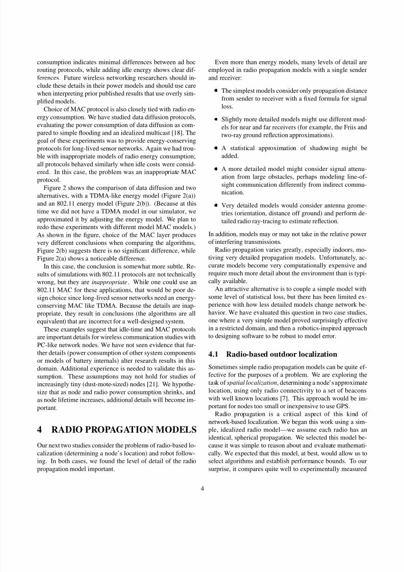
tual position. Figure 4 shows this metric from the model and
experiment. They track each other closely, including plateaus
0
2
4
6
8
10
0 2 4 6 8 10
Y ( i n m )
¥
X (in m)
ExptTheory
Median range
Figure 3: 90% radio connectivity for a transmitter at (0,0)
5
8/2/2019 He Idem Ann A
http://slidepdf.com/reader/full/he-idem-ann-a 6/10
0
20
40
60
80
100
0 0.5 1 1.5 2 2.5 3 3.5 4 4.5
C u m u l a t i v e P r o b a
b i l i t y ( % )
Localization Error (m)
theoryexperiment
Figure 4: A comparison of localization error with spherical
and experimental propagation.
is the error levels, although spherical model is consistently
slightly optimistic.
From these experiments we conclude that very simple
propagation models can be effective when simulating proto-
cols in restricted domains. We caution that this approxima-
tion is not appropriate for indoors (as would be expected)
where reflection and occlusion is common. Our indoors
measurements of propagation range varied widely from 4.6–
22.3m depending on walls and exact node locations and ori-
entations. The validated outdoor model allows us to explore a
much wider range of scenarios through simulation than could
be done through physical experimentation.
More generally, this example shows that in some cases
application-level metrics (such as localization error) are not
strongly influenced by lack of detail in lower-level simula-
tion components. In this case, it is because this approach to
proximity-based localization has an inherent measurement er-
ror that is much larger than the inaccuracy our simple outdoor
radio propagation model. We conclude that when the appli-
cation is insensitive to detail, abstract simulations can be ef-
fectively applied.
4.2 Radio-based robot following
A central challenge to practical robotics is coping with er-
ror in robotic interactions with the real world. Robotic sen-
sors are noisy and actuators (wheels, etc.) often inaccurate.
One approach to accommodate these many sources of envi-
ronmental error is to design very robust algorithms. Instead
of trying to develop very detailed models the physics of robot
movement, one approach to robotics simulation is to employ
a simple model with large amounts of random error [19]. We
believe this philosophy is also applicable in networking: net-
0
0.2
0.4
0.6
0.8
1
0 1 2 3 4 5 6 7 8 9 10
S u c c e s s P r o b a b
i l i t y
¦
Transmitter-Receiver Distance (m)
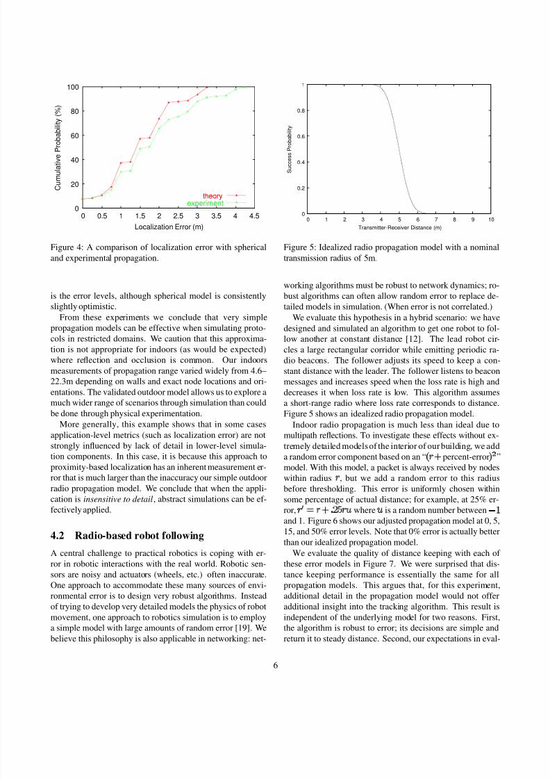
Figure 5: Idealized radio propagation model with a nominal
transmission radius of 5m.
working algorithms must be robust to network dynamics; ro-
bust algorithms can often allow random error to replace de-
tailed models in simulation. (When error is not correlated.)
We evaluate this hypothesis in a hybrid scenario: we have
designed and simulated an algorithm to get one robot to fol-
low another at constant distance [12]. The lead robot cir-
cles a large rectangular corridor while emitting periodic ra-
dio beacons. The follower adjusts its speed to keep a con-
stant distance with the leader. The follower listens to beacon
messages and increases speed when the loss rate is high and
decreases it when loss rate is low. This algorithm assumes
a short-range radio where loss rate corresponds to distance.
Figure 5 shows an idealized radio propagation model.
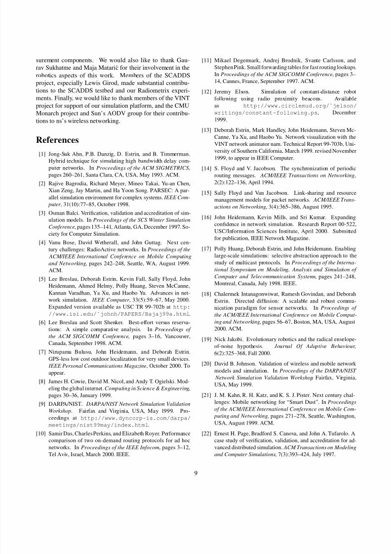
Indoor radio propagation is much less than ideal due to
multipath reflections. To investigate these effects without ex-
tremely detailed modelsof the interior of our building, we add
a random error component based on an “ §¨ percent-error
”
model. With this model, a packet is always received by nodes
within radius ¨ , but we add a random error to this radius
before thresholding. This error is uniformly chosen within
some percentage of actual distance; for example, at 25% er-
ror, ¨ ¨ ! # % ¨ (
where ( is a random number between 01
and 1. Figure 6 shows our adjusted propagation model at 0, 5,
15, and 50% error levels. Note that 0% error is actually better
than our idealized propagation model.We evaluate the quality of distance keeping with each of
these error models in Figure 7. We were surprised that dis-
tance keeping performance is essentially the same for all
propagation models. This argues that, for this experiment,
additional detail in the propagation model would not offer
additional insight into the tracking algorithm. This result is
independent of the underlying model for two reasons. First,
the algorithm is robust to error; its decisions are simple and
return it to steady distance. Second, our expectations in eval-
6

8/2/2019 He Idem Ann A
http://slidepdf.com/reader/full/he-idem-ann-a 7/10
0
0.2
0.4
0.6
0.8
1
0 1 2 3 4 5 6 7 8 9 10
S u c c e s s P r o b a b
i l i t y
¦
Transmitter-Receiver Distance (m)
No Error5% Distance Error
15% Distance Error50% Distance Error
Figure 6: The “ §¨
percent-error” propagation model used
for simulation.
0
0.2
0.4
0.6
0.8
1
0 0.5 1 1.5 2 2.5 3 3.5 4 4.5 5
C u m u l a t i v e F r e q u e n c y o f E r r o r
Drift From Desired Following Distance (meters)
Perfect Radio Model5% Error Radio Model
15% Error Radio Model50% Error Radio Model
Figure 7: Cumulative distribution of error in following dis-
tance for the four radio models.
uating this algorithm allow error; reasonably close following
(within a meter) most of the time (90%) is good.
This experiment suggests that qualitative evaluations of ap-
plications are robust to error can tolerate abstract models of
underlying layers. We would like to further verify this claim
by repeating this experiment with physical robots.
This result is not specific to robotics; we have observed
similar results in experiments involving wired networks and
the SRM protocol [15]. SRM has the same properties as our
robot-following algorithm: it uses randomized algorithms to
repair lost messages, and it can be evaluated by counting
numbers of duplicate repair messages. We have found that
the number of duplicate repairs is similar both with detailed
hop-by-hop network simulations and with abstract simula-
tions that simulate only end-to-end delay [17].
5 VISUALIZATION OF WIRELESS
SIMULATIONS
Finally, we consider the effect of details in visualization.
We have developed nam as a generic tool for visualizing theoutput of network simulations [13]. We find visualization a
very important tool for protocol debugging, but there is need
to control the amount of detail presented to the user. In this
suggestion we examine ways we use visualization to control
details, and ways that visualization is helpful at selecting the
right level of detail for wireless simulation.
Easy-to-use visualization alone provides a huge step pro-
viding a large amount of detailed information in a manage-
able fashion. Visual representations of packet flow succinctly
capture high-level information about traffic rates, congestion,
sources and destinations, and interactions for manynodes and
links. Determining the same information from textual packet
traces for a single node or link is much more difficult. Oncehot spots or problem areas are visually identified, traces can
be examined to extract specific information. We strongly en-
courage simulation authors to visualize their protocols early
in developmentto aiddebugging, and the use of a generic tool
like nam can reduce this effort.
Recent work in data diffusion provides one example of the
importance of visualization [18]. Our early experiments with
data diffusion employed a very high traffic load (a large frac-
tion of network capacity). This resulted in MAC-layer time-
outs and anomalous behavior completely unrelated to the pro-
tocol we were studying simply because we were out of an
acceptable operating region. This status would have quickly
and easily been determined from a protocol visualization, butwas lost in the aggregate statistics we considered.
Even with visualizations, the detail can become over-
whelming. We are exploring two ways to control this detail
in nam. First, we provide different kinds of visualization for
different kinds of wireless communication. Second, we allow
the user to control the level of detail nam presents.
Nam has two ways to visualize wireless communications.
First, we can visualize packet flow as rectangles that are an-
imated and move directly from the source to destination (the
lines from node 1 to nodes 2 and 3 in Figure 8). This rep-
resentation has evolved from nam’s use to visualize wired
point-to-point networks where packets flow on links. This ap-proach clearly identifies the sender and receiver of the packet,
the direction of packet flow, and the time of transmission and
receipt. However, this visualization does not easily adapt to
support broadcast traffic. Representing a broadcast packet as
multiple rectangles visually suggests multiple packets. This
approach also does not easily show when concurrent trans-
missions from different nodes interfere with each other.
An alternate visualization approach is to show wireless
packets as expanding circles (the circles in Figure 8). This
7

8/2/2019 He Idem Ann A
http://slidepdf.com/reader/full/he-idem-ann-a 8/10
Figure 8: Wireless visualization in nam
clearly shows the packet source and interference with other
packets, but it does not show destinations. If the rings disap-
pear or fade with distance, it also shows nominal radio range.
Currently we use both approaches in nam: unicast packets are
sent using rectangles, while broadcasts are sent with expand-ing circles.
In addition to choosing between two visualization meth-
ods, we allow the user to control the level of detail presented.
We are adding support for both transport- and MAC-level
trace collection in ns. Transport-level traces show packets
traveling from sources to destinations; MAC-level traces add
MAC-layer retransmits and losses. Users of nam can also
select and filter data at run-time, focusing on data for a par-
ticular sender, receiver, flow, packet-type, or similar charac-
teristics.
6 RELATED WORK
The wired networking world has depended on years of ex-
perience to guide detail in networking simulations. Ahn et
al. were the first to suggest explicitly using abstract repre-
sentations of packet trains to speed simulation [1]. Huang
et al. have examined the use of selective levels of detail
or abstraction in wired multicast simulations, and demon-
strated that abstraction causes minimal changes to SRM eval-
uations [17]. Our work differs from this work in focusing on
the relatively unexplored area of fidelity of wireless simula-
tions.
The difficulty of radio propagation has long forced the
wireless networking community to multiple levels of detail.
Recently the community has focused on the question of vali-
dation and levels of detail in wireless simulations at events
such as the DARPA/NIST Network Simulation ValidationWorkshop [9, 16]. Although some studies have compared
wireless simulations with real-world experiments (for exam-
ple, Johnson [20] for wireless ad hoc routing), there is still
relatively little experience in this area. Our work builds on
this prior work by examining five different case studies in
wireless networking.
Of course, simulation validation has its roots in general
simulation and other domains. Some recent work in the
area includes defense applications [22, 3]. Our work can
be thought of as applying these techniques in the context of
wireless networking. Our work is similar to Jakobi’s work
in robotics simulations [19] in that we are exploring the sub-
stitution of randomized noise for systematic environmental
noise. Unlike his work we are investigating that hypothesis
for wireless networking.
7 CONCLUSIONS
Choosing the right level of detail for network simulation is
difficult. Since the networking community has less experi-
ence in the wireless domain than with wired networks, choos-
ing abstractions there is even more difficult.
There are risks both in simulating with too much detail
or too little. Too much detail results in slow simulations
and cumbersome simulators. A very detailed simulation
may accurately predict today’s performance, but it may not
predict tomorrows protocol variations or be easily adapt to
quickly explore alternatives. Simulations which lack neces-
sary details can result in misleading or incorrect answers. Re-
searchers must chose their levelof simulation detailwith care.
We have offered several case studies in wireless network
simulation to offer guidance for when detail is or is not re-
quired. Even when examples are not directly applicable, sim-
ilar validation approaches may be. We have also suggested
two approaches to cope with varying levels of detail. When
error is not correlated, networking algorithms that are robust
to a range of errors are often stressed in similar ways by ran-dom error as by detailed models. Finally, visualization tech-
niques can help pinpoint incorrect details and control detail
overload.
ACKNOWLEDGMENTS
We would like to thank Nader Salehi for his contributions to
early discussions of this paper, particularly the energy mea-
8
8/2/2019 He Idem Ann A
http://slidepdf.com/reader/full/he-idem-ann-a 9/10
surement components. We would also like to thank Gau-
rav Sukhatme and Maja Mataric for their involvement in the
robotics aspects of this work. Members of the SCADDS
project, especially Lewis Girod, made substantial contribu-
tions to the SCADDS testbed and our Radiometrix experi-
ments. Finally, we would like to thank members of the VINTproject for support of our simulation platform, and the CMU
Monarch project and Sun’s AODV group for their contribu-
tions to ns’s wireless networking.
References
[1] Jong-Suk Ahn, P.B. Danzig, D. Estrin, and B. Timmerman.
Hybrid technique for simulating high bandwidth delay com-
puter networks. In Proceedings of the ACM SIGMETRICS,
pages 260–261, Santa Clara, CA, USA, May 1993. ACM.
[2] Rajive Bagrodia, Richard Meyer, Mineo Takai, Yu-an Chen,
Xian Zeng, Jay Martin, and Ha Yoon Song. PARSEC: A par-
allel simulation environment for complex systems. IEEE Com-
puter , 31(10):77–85, October 1998.
[3] Osman Balci. Verification, validation and accreditation of sim-
ulation models. In Proceedings of the SCS Winter Simulation
Conference, pages 135–141, Atlanta, GA, December 1997. So-
ciety for Computer Simulation.
[4] Vanu Bose, David Wetherall, and John Guttag. Next cen-
tury challenges: RadioActive networks. In Proceedings of the
ACM/IEEE International Conference on Mobile Computing
and Networking, pages 242–248, Seattle, WA, August 1999.
ACM.
[5] Lee Breslau, Deborah Estrin, Kevin Fall, Sally Floyd, John
Heidemann, Ahmed Helmy, Polly Huang, Steven McCanne,
Kannan Varadhan, Ya Xu, and Haobo Yu. Advances in net-
work simulation. IEEE Computer , 33(5):59–67, May 2000.
Expanded version available as USC TR 99-702b at http:
//www.isi.edu/˜johnh/PAPERS/Bajaj99a.html.
[6] Lee Breslau and Scott Shenker. Best-effort versus reserva-
tions: A simple comparative analysis. In Proceedings of
the ACM SIGCOMM Conference, pages 3–16, Vancouver,
Canada, September 1998. ACM.
[7] Nirupama Bulusu, John Heidemann, and Deborah Estrin.
GPS-less low cost outdoor localization for very small devices.
IEEE Personal Communications Magazine, October 2000. To
appear.
[8] James H. Cowie, David M. Nicol, and Andy T. Ogielski. Mod-
eling the global internet. Computing in Science & Engineering,pages 30–36, January 1999.
[9] DARPA/NIST. DARPA/NIST Network Simulation Validation
Workshop. Fairfax and Virginia, USA, May 1999. Pro-
ceedings at http://www.dyncorp-is.com/darpa/
meetings/nist99may/index.html.
[10] Samir Das, CharlesPerkins, and Elizabeth Royer. Performance
comparison of two on-demand routing protocols for ad hoc
networks. In Proceedings of the IEEE Infocom, pages 3–12,
Tel Aviv, Israel, March 2000. IEEE.
[11] Mikael Degermark, Andrej Brodnik, Svante Carlsson, and
StephenPink. Small forwarding tables for fast routinglookups.
In Proceedings of the ACM SIGCOMM Conference, pages 3–
14, Cannes, France, September 1997. ACM.
[12] Jeremy Elson. Simulation of constant-distance robot
following using radio proximity beacons. Available
as http://www.circlemud.org/˜jelson/
writings/constant-following.ps, December
1999.
[13] Deborah Estrin, Mark Handley, John Heidemann, Steven Mc-
Canne, Ya Xu, and Haobo Yu. Network visualization with the
VINT network animator nam. Technical Report 99-703b, Uni-
versity of Southern California, March 1999. revised November
1999, to appear in IEEE Computer.
[14] S. Floyd and V. Jacobson. The synchronization of periodic
routing messages. ACM/IEEE Transactions on Networking,
2(2):122–136, April 1994.
[15] Sally Floyd and Van Jacobson. Link-sharing and resourcemanagement models for packet networks. ACM/IEEE Trans-
actions on Networking, 3(4):365–386, August 1995.
[16] John Heidemann, Kevin Mills, and Sri Kumar. Expanding
confidence in network simulation. Research Report 00-522,
USC/Information Sciences Institute, April 2000. Submitted
for publication, IEEE Network Magazine.
[17] Polly Huang, Deborah Estrin, and John Heidemann. Enabling
large-scale simulations: selective abstraction approach to the
study of multicast protocols. In Proceedings of the Interna-
tional Symposium on Modeling, Analysis and Simulation of
Computer and Telecommunication Systems, pages 241–248,
Montreal, Canada, July 1998. IEEE.
[18] Chalermek Intanagonwiwat, Ramesh Govindan, and Deborah
Estrin. Directed diffusion: A scalable and robust commu-
nication paradigm for sensor networks. In Proceedings of
the ACM/IEEE International Conference on Mobile Comput-
ing and Networking, pages 56–67, Boston, MA, USA, August
2000. ACM.
[19] Nick Jakobi. Evolutionary robotics and the radical envelope-
of-noise hypothesis. Journal Of Adaptive Behaviour ,
6(2):325–368, Fall 2000.
[20] David B. Johnson. Validation of wireless and mobile network
models and simulation. In Proceedings of the DARPA/NIST
Network Simulation Validation Workshop, Fairfax, Virginia,
USA, May 1999.
[21] J. M. Kahn, R. H. Katz, and K. S. J. Pister. Next century chal-
lenges: Mobile networking for “Smart Dust”. In Proceedings
of the ACM/IEEE International Conference on Mobile Com-
puting and Networking, pages 271–278, Seattle, Washington,
USA, August 1999. ACM.
[22] Ernest H. Page, Bradford S. Canova, and John A. Tufarolo. A
case study of verification, validation, and accreditation for ad-
vanced distributed simulation. ACM Transactions on Modeling
and Computer Simulations, 7(3):393–424, July 1997.
9

8/2/2019 He Idem Ann A
http://slidepdf.com/reader/full/he-idem-ann-a 10/10
[23] Mark Stemm and Randy H. Katz. Measuring and reduc-
ing energy consumption of network interfaces in hand-held
devices. IEICE Transactions on Communications, E80-
B(8):1125–1131, August 1997.
[24] Ya Xu, John Heidemann, and Deborah Estrin. Adaptive
energy-conserving routing for multihop ad hoc networks. Sub-mitted for publication, May 2000.
10