Research ArticleNew Exact Soliton Solutions of the (3 + 1)-DimensionalConformable Wazwaz–Benjamin–Bona–Mahony Equation viaTwo Novel Techniques

Mohammed K. A. Kaabar ,1,2,3 Melike Kaplan,4 and Zailan Siri 1

1Institute of Mathematical Sciences, Faculty of Science, University of Malaya, Kuala Lumpur 50603, Malaysia2Gofa Camp near Gofa Industrial College and German Adebabay, Nifas Silk-Lafto, 26649 Addis Ababa, Ethiopia3Jabalia Camp, United Nations Relief and Works Agency (UNRWA), Palestinian Refugee Camp, Gaza Strip,Jabalya, State of Palestine4Department of Mathematics, Art-Science Faculty, Kastamonu University, Kastamonu, Turkey

Correspondence should be addressed to Mohammed K. A. Kaabar; mohammed.kaabar@wsu.eduand Zailan Siri; zailansiri@um.edu.my

Received 12 May 2021; Revised 12 June 2021; Accepted 26 June 2021; Published 22 July 2021

Academic Editor: Dumitru Vieru

Copyright © 2021 Mohammed K. A. Kaabar et al. This is an open access article distributed under the Creative CommonsAttribution License, which permits unrestricted use, distribution, and reproduction in any medium, provided the original workis properly cited.

In this work, the (3 + 1)-dimensional Wazwaz–Benjamin–Bona–Mahony equation is formulated in the sense of conformablederivative. Two novel methods of generalized Kudryashov and expð−φðℵÞÞ are investigated to obtain various exact solitonsolutions. All algebraic computations are done with the help of the Maple software. Graphical representations are provided in3D and 2D profiles to show the behavior and dynamics of all obtained solutions at various parameters’ values and conformableorders using Wolfram Mathematica.

1. Introduction

Partial differential equations (PDEqs) have attracted a partic-ular interest from researchers in the fields of natural sciencesand engineering due to the applicability of these equations inmodeling various scientific phenomena in interdisciplinarysciences such as mathematical physics, mechanics, signaland image processing, and chemistry. Most physical systemsare not linear; therefore, nonlinear partial differential equa-tions (NLPDEqs), particularly nonlinear evolution equations(NLEEqs) (see [1]), have inspired researchers to investigatethe existence of exact solutions for such equations. Findingnew exact solutions for NLPDEqs can significantly providea good interpretation for the physical meaning and dynamicsof these equations. Therefore, several research studies haverecently been done on developing new methods for solvingNLPDEqs exactly. Some of the most notable methods thathave been applied to solve some interesting NLPDEqs are

the methods of modified simple equation and extended sim-plest equation to solve (4 + 1)-dimensional nonlinear Fokasequation [2], the methods of exp-function and expð−ΦðℵÞÞ-expansion to solve Vakhnenko-Parkes equation [3], andthe method of generalized Kudryashov to solve nonlinearJaulent-Miodek hierarchy and (2 + 1)-dimensional Calogero-Bogoyavlenskii-Schiff equations [4]. To solve nonlinear inte-grable equations, a novel technique, known as Hirota bilinearmethod, was proposed byMa andMa et al. in [5, 6] in order toobtain new lump solutions for the investigated equations [7].

One of the most interesting NLPDEqs is the Benjamin-Bona-Mahony equation (BBMEq), an extension of theKorteweg-de Vries equation (KdVEq), which is basically amodel that represents the unidirectional propagation of longwaves with small amplitude on the hydromagnetic andacoustic waves’ surface in shallow water channel [8, 9]. Con-sider the following (3 + 1)-dimensional modified form ofBBMEq:

HindawiJournal of Function SpacesVolume 2021, Article ID 4659905, 13 pageshttps://doi.org/10.1155/2021/4659905

Ψt +Ψx +Ψ2Ψy −Ψyzt = 0: ð1Þ

Equation (1) was first proposed by Wazwaz [10] by for-mulating a new three-dimensional modified version ofBBMEqs, known as the Wazwaz-Benjamin-Bona-Mahonyequation (WBBMEq), via coupling or various generalizedcontexts or as combination of both of them. Higher dimen-sional problems with various applications can be describedby the WBBMEq with its spatial and temporal variables [8,9]. Therefore, there is a significant need to find exact solu-tions for WBBMEq to interpret their physical meaning anddynamics.

Fractional differential equations (FDiEqs) are generalizedforms of integer-order differential equations. FDiEqs haveattracted the interests of researchers due to the ability of theseequations in modeling various scientific phenomena betterthan the integer-order ones (refer to [11–13]). The behaviorof some physical systems can be interpreted better than theinteger-order ones due to the nonlocality of fractional deriv-atives, and many systems have memory effects. There aremany definitions of fractional derivatives, but the most com-mon ones are Riemann-Liouville and Caputo fractionalderivatives where the properties of linearity are commonlyshared among these derivatives, but other properties suchas product rule, constant, chain rule, and quotient rule arenot satisfied. FDiEqs are considered as a powerful tool inmodeling scenarios (see [14–16]), but this tool comes withvarious challenges when dealing with FDiEqs due to the dif-ficulty of obtaining exact or analytical solutions where thesolutions can be very complicated or impossible to obtainthem for certain cases. As a result, to overcome some of chal-lenges associated with nonlocal fractional derivatives, a newgeneralized fractional derivative of local-type, named con-formable derivative, was proposed by Khalil et al. which isbasically a stretch for the usual limit-based definition whereall usual derivative’s properties are satisfied [17]. Manyresearch studies have discussed the mathematical analysisand applications of conformable derivative such as conform-able Laplace’s equation [18] and generalized conformablemean value theorems [19].

Seadawy et al. [20] and Bilal et al. [21] investigated vari-ous soliton solutions for conformable WBBMEq using themethods of simple ansatz and generalized exponential ratio-nal function, respectively.

Inspired by all above studies, this work is mainly aimed atobtaining new exact solitary solutions for a version ofWBBMEq formulated in the sense of conformable derivative(ComD) with the help of two novel techniques: generalizedKudryashov method and expð−φðℵÞÞ method. The generalfractional formulation of WBBMEq can be expressed as fol-lows:

DζtΨ +Dζ

xΨ +DζyΨ −D3ζ

xztΨ = 0, ð2Þ

where Dζ is the fractional operator of order: ζ ∈ ð0, 1�. Theexact solutions of Eq. (2) have been investigated in someresearch works using the ðG′/GÞ-expansion method [9],modified simple equation method [8], and Riccati-Bernoulli

Sub-ODE method [8]. However, according to the best ofour knowledge, none of previous research works has investi-gated Eq. (2) in the context of ComD via the methods of gen-eralized Kudryashov and expð−φðℵÞÞ.

Therefore, all results in our work are new and worthy.This work is divided into the following sections: Essential

notions about conformable derivative are presented, and themethodology of our two proposed approaches is discussed inSection 2. In Section 3, the main results of our work are pre-sented. In Section 4, the graphical comparisons of ourobtained exact solutions are represented in both 2D and 3Dplots for various values of parameters and ζ. The conclusionof our work is provided in Section 5.

2. Fundamental Preliminaries andMethodology

Some important notions about conformable derivative areintroduced in this section. In addition, the methodology oftwo different approaches, namely, generalized Kudryashovmethod and expð−φðℵÞÞ method, is also described, respec-tively. The conformable derivative can be defined as follows:

Definition 1. Given a function Ψ : ½0,∞Þ⟶R ∋ ∀t > 0, theconformable derivative of order ζ ∈ ð0, 1� of Ψ can beexpressed as follows:

Dζt Ψ tð Þð Þ = lim

Ω⟶0

Ψ t +Ωt1−ζ� �

−Ψ tð ÞΩ

: ð3Þ

Let Ψ be ζ-differentiable in some ð0, ϱÞ, where ϱ > 0, andthe limit of Dζ

t ðΨðtÞÞ exists as t⟶ 0+; then, from this defi-nition, we obtain the following:

Dζt Ψ 0ð Þð Þ = lim

t⟶0+Dζt Ψ tð Þð Þ: ð4Þ

The theorem [17] below shows that Dζt satisfies all usual

limit-based derivative’s properties as follows:

Theorem 2. For ζ ∈ ð0, 1�, let functions Ψ and Φ be ζ-differ-entiable at a point t; then, we have the following:

(a) Dζt ðΨðtÞΦðtÞÞ =ΨðtÞDζ

t ðΦðtÞÞ +ΦðtÞDζt ðΨðtÞÞ

(b) Dζt ðmΨðtÞ +wΦðtÞÞ =mDζ

tΨðtÞ +wDζtΦðtÞ, ∀m,w

∈R

(c) Dζt ðΨðtÞ/ΦðtÞÞ =ΦðtÞDζ

t ðΨðtÞÞ − ðΨðtÞÞDζt ðΦðtÞÞ/Φ2ðtÞ

(d) Dζt ðtkÞ = ktk−ζ, ∀k ∈R

(e) If ΨðtÞ is assumed to be a differentiable function,thenDζ

t ðΨðtÞÞ = t1−ζdΨ/dt

(f) Dζt ðνÞ = 0, ∀constant functionsΨðtÞ = ν

The methodology of the generalized Kudryashov method(GKuM) and expð−φðℵÞÞ method (ExpM) can be presentedas follows:

2 Journal of Function Spaces

Consider the following form of NLEEq, with 4 indepen-dent variables: x, y, z, and t, formulated generally in the senseof fractional derivative:

T Ψ,DζtΨ,Dζ

xΨ,DζyΨ,Dζ

zΨ,D2ζt Ψ,D2ζ

x Ψ,D2ζy Ψ,D2ζ

z Ψ,⋯� �= 0 ; 0 < ζ ≤ 1,

ð5Þ

where Ψ =Ψðx, y, z, tÞ is an unknown function and T is apolynomial of Ψ and its partial derivatives in which all ofthe nonlinear terms and highest-order derivatives areincluded in Eq. (5). First of all, to solve Eq. (5), we use the fol-lowing traveling wave transformations for ComD:

For ComD,

Ψ x, y, z, tð Þ =Ψ ℵð Þ ;ℵ = pxζ

ζ+ q

yζ

ζ+ γ

zζ

ζ− δ

tζ

ζ, ð6Þ

where p, q, γ, and δ are all constants with the condition: p,q, γ, δ ≠ 0, and δ is the wave speed.

According to the above transformations, Eq. (5) isreduced to the following ODE.

L Ψ,Ψ′,Ψ′′,Ψ′′′,⋯� �

= 0: ð7Þ

The derivative with respect to ℵ is represented by aprime. Equation (7) should be integrated term by term oneor more times.

2.1. The Generalized Kudryashov Method. From GKuM, theobtained solution for the reduced equation is constructedby a polynomial in ℏðℵÞ as [4, 22]:

Ψ ℵð Þ = ∑Jk=0pkℏ

k ℵð Þ∑W

l=0qlℏl ℵð Þ

, ð8Þ

where pkðk = 0, 1,⋯, jÞ, blðl = 0, 1,⋯,wÞ are constantswhich are needed to be determined ∍pJ ≠ 0, qW ≠ 0, and L =LðℵÞ is the solution of the following equation:

dℏdℵ

= ℏ2 ℵð Þ − ℏ ℵð Þ: ð9Þ

The solution of Eq. (9) can be expressed as follows:

ℏ ℵð Þ = 11 + I1eℵ

, ð10Þ

where I1 is an integration constant.According to the homogeneous balance principle

(HBPrp), the positive integers: J and W in Eq. (8) can beobtained with the help of Eq. (7). In addition, a polynomial,ℏ, can be determined by the substitution of Eq. (8) into Eq.(7) along with Eq. (9). Now, by equating all the coefficientsof polynomial ℏ to 0 in order to construct a system of alge-braic equations, this system is solved with the aid of the com-

puter software such as Maple and Wolfram Mathematicain order to find the values of pkðk = 0, 1,⋯, jÞ, qlðl = 0, 1,⋯,wÞ. At the end, all soliton-type solutions of the reducedEq. (7) can be found by the substitution of these obtainedvalues and Eq. (9) into Eq. (8).

2.2. The expð−φðℵÞÞ Method. From ExpM [3], the obtainedsolution for the reduced equation is constructed by a polyno-mial in expð−ΦðℵÞÞ as follows:

Ψ ℵð Þ = 〠w

j=0pj exp −ϕ ℵð Þð Þð Þj, ð11Þ

where pjðpw ≠ 0Þ are constants which are needed to be found,and φðℵÞ satisfies the following auxiliary ODE:

φ′ ℵð Þ = exp −φ ℵð Þð Þ + ϑ exp φ ℵð Þð Þ + χ: ð12Þ

Note that Eq. (12) has distinct solutions which areexpressed as follows:

Case 1. When χ2 − 4ϑ > 0 and ϑ ≠ 0, the hyperbolic functionsolutions are expressed as follows:

ϕ1 ℵð Þ = ln−

ffiffiffiffiffiffiffiffiffiffiffiffiffiffiχ2 − 4ϑ

ptanh

ffiffiffiffiffiffiffiffiffiffiffiffiffiffiffiffiffiffiχ2 − 4ϑ/2

pℵ + Ið Þ

� �− χ

2ϑ

0@

1A: ð13Þ

Case 2. When χ2 − 4ϑ < 0 and ϑ ≠ 0, the trigonometric func-tion solutions are expressed as follows:

ϕ2 ℵð Þ = lnffiffiffiffiffiffiffiffiffiffiffiffiffiffi4ϑ − χ2

ptan

ffiffiffiffiffiffiffiffiffiffiffiffiffiffiffiffiffiffi4ϑ − χ2/2

pℵ + Cð Þ

� �− χ

2ϑ

0@

1A: ð14Þ

Case 3. When χ2 − 4ϑ > 0, ϑ = 0 and χ ≠ 0, the hyperbolicfunction solutions are expressed as follows:

ϕ3 ℵð Þ = − ln χ

cosh χ ℵ + Ið Þð Þ + sinh χ ℵ + Ið Þð Þ − 1

� �: ð15Þ

Case 4. Whenχ2 − 4ϑ = 0, ϑ ≠ 0 and χ ≠ 0, the rational func-tion solutions are expressed as follows:

ϕ4 ℵð Þ = ln −2 χ ℵ + Ið Þ + 2ð Þ

χ2 ℵ + Ið Þ� �

: ð16Þ

Case 5. When χ2 − 4ϑ = 0, ϑ = 0 and χ = 0, we have the fol-lowing:

φ5 ℵð Þ = ln ℵ + Ið Þ: ð17Þ

From the above cases, the integration constant is repre-sented by I. By the substitution of Eq. (11) into the reducedEq. (7) and collecting all terms together that are in the sameorder of expð−φðℵÞÞjðj = 0, 1, 2,⋯Þ, the polynomial in termsof expð−φðℵÞÞ is verified. Then, by equating all coefficients to0, a set of algebraic equations is constructed for pjðj = 0, 1, ::

3Journal of Function Spaces

mÞ, χ, δ and ϑ. With the help of Maple, Walfram Mathema-tica, or MATLAB, the system can be solved to obtain diverseexact solutions for Eq. (6).

3. Solutions of the (3 + 1)-DimensionalConformable WBBMEq

Exact soliton solutions of the proposed Eq. (2) are obtainedin this section via GKuM and ExpM.

pγδΨ′′′ + q Ψ3� �′ + −γ + pð ÞΨ′ = 0: ð18Þ

By integrating Eq. (18) once with respect to ℵ, we obtainthe following:

pγδΨ″ + qΨ3 −δ + pð ÞΨ = 0: ð19Þ

3.1. Exact Solutions via the Generalized Kudryashov Method.According to the HBPrp, it is obvious to have J =W + 1. Letus set W = 1, and we obtain J = 2. Thus, the solution can bewritten as follows:

Ψ ℵð Þ = p0 + p1ℏ+p2ℏ2q0 + q1ℏ

, ð20Þ

where ℏ = ℏðℵÞ is the solution of Eq. (9). As a result, bysubstituting Eq. (20) into Eq. (19) and using Eq. (9), weobtain system of algebraic equations by equating all coeffi-cients of the functions ℏ0, ℏ1, ℏ2, ℏ3, ℏ4, ℏ5, ℏ6 to 0. Now, p0,p1, p2, q0, and q1 are all parameters.

ℏ6 : qp32 + 2pγδp2q21 = 0,ℏ5 : 3qp1p22 − 3pγδp2q21 + 6pγδp2q0q1 = 0,ℏ4 : −9pγδp2q0q1 − δp2q

21 + pp2q

21 + 6pγδp2q20

+ pγδp2q21 + 3qp0p22 + 3qp21p2 = 0,

ℏ3 : −δp1q21 + 2pγδp1q20 + qp31 − 10pγδp2q20

+ pγδℏ1q0q1 − pγδq21p0 + pp1q21 − 2δp2q0q1

+ 3pγδp2q0q1 + 6qp0p1p2 + 2pp2q0q1− 2pγδq1p0q0 = 0,

ℏ2 : −2δp1q0q1 − pγδp1q0q1 + pp0q21 + 3qp20p2

− δp0q21 + 3qp0p21 − 3pγδp1q20 + 2pp1q0q1

+ pp2q20 − δp2q

20 + 4pγδp2q20 + pγδq21p0

+ 3pγδq1p0q0 = 0,

ℏ1 : −pγδq1p0q0 + 2pp0q0q1 + pγδp1q20 − δp1q

20

+ 3qp20p1 − 2δp0q0q1 + pp1q20 = 0,

ℏ0 : pp0q20 + qp30 = 0:

ð21Þ

From the above set of algebraic equations, various casesare presented as follows:

Case 1.

p0 = 0, p1 = ±pq1ffiffiffiffiffiffiffiffiffiffiffiffiffiffiffiffiffiffiffiffi−

γ

2q + pqγ

r,

p2 = ± 2pγq1pγ + 2ð Þq ffiffiffiffiffiffiffiffiffiffiffiffiffiffiffiffiffiffiffiffiffiffiffiffi

−γ/2q + pqγp ,

q0 = 0, q1 = q1, δ =2p

pγ + 2 :

ð22Þ

Then, by the substitution of the obtained values into Eq.(20) with Eq. (10), the soliton-type solutions of the followingWBBMEq in the sense of ComD are as follows:

where ℵ = pðxς/ςÞ + qðyς/ςÞ + γðzς/ςÞ − ð2p/pγ + 2Þtς/ς forComD. I1 is an arbitrary constant.

Case 2.

p0 = 0, p1 = ±2q0pffiffiffiffiffiffiffiffiffiffiffiffiffiffiffiffiffi

2γ−q + pqγ

s,

p2 = ∓2q0pffiffiffiffiffiffiffiffiffiffiffiffiffiffiffiffiffi

2γ−q + pqγ

s,

q0 = q0, q1 = −2q0, δ =p

1 − pγ:

ð24Þ

Then, by the substitution of the obtained values into Eq.(20) with Eq. (10), the soliton-type solutions of the followingWBBMEq in the sense of ComD are as follows:

Ψ2 x, y, z, tð Þ

= ± 2pI1ffiffiffiffiffiffiffiffiffiffiffiffiffiffiffiffiffiffiffiffiffiffiffiffiffiffiffi2γ/q −1 + pγð Þp

cosh ℵð Þ + sinh ℵð Þð Þ−1 + I21 2 cosh ℵð Þ sinh ℵð Þ + 2 cosh2 ℵð Þ − 1

� � ,ð25Þ

where ℵ = pðxς/ςÞ + qðyς/ςÞ + γðzς/ςÞ − ðp/1 − pγÞtς/ς forComD. I1 is a constant.

Ψ1 x, y, z, tð Þ = ± 1 − I1 cosh ℵð Þ + sinh ℵð Þð Þð Þpγffiffiffiffiffiffiffiffiffiffiffiffiffiffiffiffiffiffiffiffiffiffiffiffiffi−γ/q pγ + 2ð Þp

q pγ + 2ð Þ 1 + I1 cosh ℵð Þ + I1 sinh ℵð Þð Þð Þ, ð23Þ

4 Journal of Function Spaces

3.2. Exact Solutions via the expð−φðℵÞÞMethod. The ExpM isa very helpful technique to construct the solution of Eq. (7) inthe following form:

Ψ ξð Þ = p0 + p1 exp −φ ℵð Þð Þ: ð26Þ

Let us substitute Eq. (19) into Eq. (7) and collect the coef-ficient of each power of expð−ΦðℵÞÞj. Now, a set of algebraicequations of p, q, γ, δ, p0, p1, χ and ϑ is obtained by equatingall coefficients to 0.

exp 3ℵð Þ: qp30δp0 + pγδp1ϑχ + pp0 = 0,exp 2ℵð Þ: 3qp20p1 − δp1 + 2pγδp1ϑ + pγδp1χ

2 + pp1 = 0,exp ℵð Þ: 3pγδp1χ + 3qp0p21 = 0,

exp 0ℵð Þ: 2pγδp1 + qp31 = 0:ð27Þ

With the help of software programs such as Maple orMathematica, the solution is obtained as follows:

p0 = ±χpffiffiffiffiffiffiffiffiffiffiffiffiffiffiffiffiffiffiffiffiffiffiffiffiffiffiffiffiffiffiffiffiffiffiffiffiffiffiffiffiffi

γ

−pqγχ2 − 2q + 4pqγϑ

r,

p1 = ±2pffiffiffiffiffiffiffiffiffiffiffiffiffiffiffiffiffiffiffiffiffiffiffiffiffiffiffiffiffiffiffiffiffiffiffiffiffiffiffiffiffi

γ

−pqγχ2 − 2q + 4pqγϑ

r,

δ = 2ppγχ2 + 2 − 4pγϑ :

ð28Þ

From all the above obtained values, the technique’s algo-rithm, and its auxiliary equations, different cases for the con-formable WBBMEq are given as follows:

Case 1. When χ2 − 4ϑ > 0 and ϑ ≠ 0, the hyperbolic functionsolutions are expressed as follows:

where ℵ = pðxς/ςÞ + qðyς/ςÞ + γðzς/ςÞ − ð2p/pγχ2 + 2 − 4pγϑÞtς/ς for ComD. I is a constant.

Case 2. When χ2 − 4ϑ < 0 and ϑ ≠ 0, the trigonometric func-tion solutions are expressed as follows:

where ℵ = pðxς/ςÞ + qðyς/ςÞ + γðzς/ςÞ − ð2p/pγχ2 + 2 − 4pγϑÞtς/ς for ComD. I is a constant.

Case 3. When χ2 − 4ϑ > 0, ϑ = 0 and χ ≠ 0, the hyperbolicfunction solutions are expressed as follows:

where ℵ = pðxς/ςÞ + qðyς/ςÞ + γðzς/ςÞ − ð2p/pγχ2 + 2 − 4pγϑÞtς/ς for ComD. I is a constant.

Case 4. When χ2 − 4ϑ = 0, ϑ ≠ 0 and χ ≠ 0, the rational func-tion solutions are expressed as follows:

Ψ4 x, y, z, tð Þ = ± 2χpffiffiffiffiffiffiffiffiffiffiffiffiffiffiffiffiffiffiffiffiffiffiffiffiffiffiffiffiffiffiffiffiffiffiffiffiffiffiffiffiffiffiffiffiγ/q −pγχ2 − 2 + 4pγϑð Þpχ ℵ + Ið Þ + 2 , ð32Þ

where ℵ = pðxς/ςÞ + qðyς/ςÞ + γðzς/ςÞ − ð2p/pγχ2 + 2 − 4pγϑÞtς/ς for ComD. I is a constant.

Case 5. Finally, when χ2 − 4ϑ = 0, ϑ = 0 and χ = 0, we have thefollowing:

Ψ5 x, y, z, tð Þ = ±ffiffiffiffiffiffiffiffiffiffiffiffiffiffiffiffiffiffiffiffiffiffiffiffiffiffiffiffiffiffiffiffiffiffiffiffiffiffiffiffiffiffiffiffiγ/q −pγχ2 − 2 + 4pγϑð Þp

p χ ℵ + Ið Þ + 2ð Þℵ + I

,

ð33Þ

Ψ1 x, y, z, tð Þ = ±p

ffiffiffiffiffiffiffiffiffiffiffiffiffiffiffiffiffiffiffiffiffiffiffiffiffiffiffiffiffiffiffiffiffiffiffiffiffiffiffiffiffiffiffiffiγ/q −pγχ2 − 2 + 4pγϑð Þp

χ2 + χ tanhffiffiffiffiffiffiffiffiffiffiffiffiffiffiffiffiffiffiχ2 − 4ϑ/2

pℵ + Ið Þ

� � ffiffiffiffiffiffiffiffiffiffiffiffiffiffiχ2 − 4ϑ

p− 4ϑ

� �χ + tanh

ffiffiffiffiffiffiffiffiffiffiffiffiffiffiffiffiffiffiχ2 − 4ϑ/2

pℵ + Ið Þ

� � ffiffiffiffiffiffiffiffiffiffiffiffiffiffiχ2 − 4ϑ

p , ð29Þ

Ψ2 x, y, z, tð Þ = ±p

ffiffiffiffiffiffiffiffiffiffiffiffiffiffiffiffiffiffiffiffiffiffiffiffiffiffiffiffiffiffiffiffiffiffiffiffiffiffiffiffiffiffiffiffiγ/q −pγχ2 − 2 + 4pγϑð Þp

−χ2 + χ tanffiffiffiffiffiffiffiffiffiffiffiffiffiffiffiffiffiffi4ϑ − χ2/2

pℵ + Ið Þ

� � ffiffiffiffiffiffiffiffiffiffiffiffiffiffi4ϑ − χ2

p+ 4ϑ

� �−χ + tan

ffiffiffiffiffiffiffiffiffiffiffiffiffiffiffiffiffiffi4ϑ − χ2/2

pℵ + Ið Þ

� � ffiffiffiffiffiffiffiffiffiffiffiffiffiffi4ϑ − χ2

p , ð30Þ

Ψ3 x, y, z, tð Þ = ±χpffiffiffiffiffiffiffiffiffiffiffiffiffiffiffiffiffiffiffiffiffiffiffiffiffiffiffiffiffiffiffiffiffiffiffiffiffiffiffiffiffiffiffiffiγ/q −pγχ2 − 2 + 4pγϑð Þp

cosh χ ℵ + Ið Þð Þ + sinh χ ℵ + Ið Þð Þ + 1ð Þcosh χ ℵ + Ið Þð Þ + sinh χ ℵ + Ið Þð Þ − 1 , ð31Þ

5Journal of Function Spaces

100

50

0100

50

0.25

0.30

0.35

0t

x

(a)

20

0.3

0.2

0.1

−0.1

−0.2

−0.3

40 60 80 100

(b)

80

60

40

20

0100

50

−0.2

0.00.20.4

0

x

t

(c)

20

0.3

0.2

0.1

−0.1

−0.2

−0.3

40 60 80 100

(d)

60

40

20

0100

50

−0.20.00.2

0.4

0

x

t

(e)

20

0.3

0.2

0.1

−0.1

−0.2

−0.3

40 60 80 100

(f)

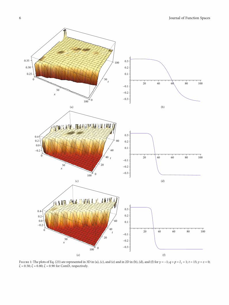
Figure 1: The plots of Eq. (23) are represented in 3D in (a), (c), and (e) and in 2D in (b), (d), and (f) for γ = −1; q = p = I1 = 1; t = 15; y = z = 0;ζ = 0:50; ζ = 0:80; ζ = 0:90 for ComD, respectively.

6 Journal of Function Spaces

where ℵ = pðxς/ςÞ + qðyς/ςÞ + γðzς/ςÞ − ð2p/pγχ2 + 2 − 4pγϑÞtς/ς for ComD. I is a constant.

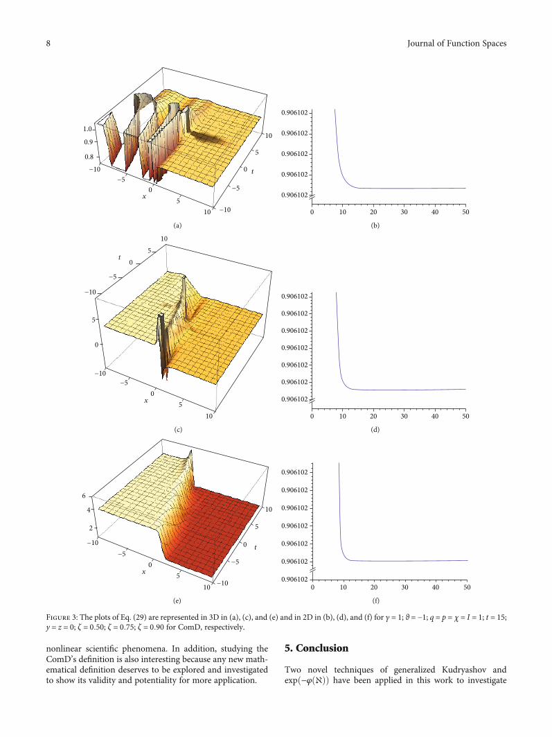
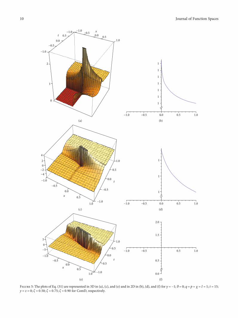
4. The Graphical Comparisons of Solutions

To show the dynamics and behavior of our obtained solu-tions, various soliton solutions in Eqs. (23), (25), (29), (30),(31), (32), and (33) are graphically represented and com-pared in both 3D and 2D plots in Figures 1–7 for variousparameters’ values and ζ. In this work, two techniques areemployed in the sense of ComD. Therefore, all our resultsare new and worthy because studying WBBMEq is veryimportant to investigate various nonlinear scientific phe-

nomena. ComD is a local-type fractional derivative which isa generalized formulation of usual limit-based derivative.Since the measurements in physics are local, this can makeComD suitable for modeling many physical phenomena,and it is also efficient to work with ComD to obtain exactsolutions for NLPDEqs although ComD does not have someof the essential properties to be categorized as a fractionalderivative. From the authors’ opinion, formulating and solv-ing NLPDEqs in the sense of ComD are always recom-mended since all local and nonlocal fractional derivativeshave both advantages and disadvantages. Therefore, explor-ing new properties and definitions for all local and nonlocalfractional derivatives are helpful while working on modeling

10

5

010

5

0.0

0.5

0

x

t

(a)

20

2

1

−1

−2

40 60 80 10

(b)

10

5

010

5

0.0−0.5

0.5

0

x

t

(c)

2

1.0

0.5

−0.5

−1.0

4 6 8 10

(d)

10

5

010

5

0.0−0.5

0.5

0

x

t

(e)

2

1.0

0.5

−0.5

−1.0

4 6 8 10

(f)

Figure 2: The plots of Eq. (25) are represented in 3D in (a), (c), and (e) and in 2D in (b), (d), and (f) for γ = −1; q = p = I1 = 1; t = 15; y = z = 0;ζ = 0:50; ζ = 0:80; ζ = 0:90 for ComD, respectively.

7Journal of Function Spaces

nonlinear scientific phenomena. In addition, studying theComD’s definition is also interesting because any new math-ematical definition deserves to be explored and investigatedto show its validity and potentiality for more application.

5. Conclusion

Two novel techniques of generalized Kudryashov andexpð−φðℵÞÞ have been applied in this work to investigate

10

5

0

−5

−1010

05

−5

0.9

0.8

1.0

−10

x

t

(a)

0.906102

0.906102

0.906102

0.906102

0.906102

0 10 20 30 40 50

(b)

10

05

−5

0

5

−10

−10

−5

0t

5

10

x

(c)

0.906102

0.906102

0.906102

0.906102

0.906102

0.906102

0.906102

0 10 20 30 40 50

(d)

10

5

0

−5

−1010

05

−5

2

4

−10

6

x

t

(e)

0.906102

0.906102

0.906102

0.906102

0.906102

0.906102

0.9061020 10 20 30 40 50

(f)

Figure 3: The plots of Eq. (29) are represented in 3D in (a), (c), and (e) and in 2D in (b), (d), and (f) for γ = 1; ϑ = −1; q = p = χ = I = 1; t = 15;y = z = 0; ζ = 0:50; ζ = 0:75; ζ = 0:90 for ComD, respectively.

8 Journal of Function Spaces

1000

500

−500

−1000

−1000

2.0

2.5

1000

−500

500

0x

t0

(a)

2.32622

0 20 40 60 80 100

2.32622

2.32622

2.32622

(b)

−10

0

5

10

−5

−5

−50

5

10

−10

50

x

t

(c)

2

1

−1000 −500 500 1000

−1

−2

(d)

−1000

−1000

−5000

0

500

1000

−500

1

2

1000

−2−10

500

0x

t

(e)

2

1

−1000 −500 500 1000

−1

−2

(f)

Figure 4: The plots of Eq. (30) are represented in 3D in (a), (c), and (e) and in 2D in (b), (d), and (f) for γ = 1; ϑ = 1; q = p = χ = I = 1; t = 15;y = z = 0; ζ = 0:50; ζ = 0:75; ζ = 0:90 for ComD, respectively.

9Journal of Function Spaces

0

1

2

−1.0

−1.0 −1.0−0.5

0.00.5

1.0

−0.50.0

0.5x

t

(a)

1

1

1

1

1

1

1

−1.0 −0.5 0.0 0.5 1.0

(b)

1.0

0.5

0.0

−0.5

−1.0

−1.0

−4

−2

0

2

4

−0.5

0.0

x

t

0.5

1.0

(c)

1

1

1

−1.0 −0.5 0.5 1.00.0

(d)

−1.0

−1.0

−0.5

−5

0

5

0.0

0.5

1.0

−0.5

0.0

0.5

1.0

x

t

(e)

−1.0 −0.5 0.5

2.0

1.5

0.5

0.0

1.0

(f)

Figure 5: The plots of Eq. (31) are represented in 3D in (a), (c), and (e) and in 2D in (b), (d), and (f) for γ = −1; ϑ = 0; q = p = χ = I = 1; t = 15;y = z = 0; ζ = 0:50; ζ = 0:75; ζ = 0:90 for ComD, respectively.

10 Journal of Function Spaces

200

200

100

0100

0

0.020.040.060.08

t

x

(a)

−500 0 500 1000−1000

0.07

0.05

0.06

0.04

0.03

0.02

(b)

0

−5

−10

t

x

−10−0.2

−0.1

0.0

−5

0

(c)

−500 0 500 1000−1000

0.04

0.03

0.02

0.01

(d)

−10

−10

−0.6−0.4−0.20.00.2

−5

−5

0

0

t

x

(e)

−500 500 1000−1000

0.025

0.020

0.015

0.005

0.010

(f)

Figure 6: The plots of Eq. (32) are represented in 3D in (a), (c), and (e) and in 2D in (b), (d), and (f) for γ = 1; ϑ = 0; q = p = χ = I = 1; t = 15;y = z = 0; ζ = 0:50; ζ = 0:75; ζ = 0:90 for ComD, respectively.

11Journal of Function Spaces

−50

−100

−100

100

50

0

−50

0.00

0.02

0.04

0.06

100

50

0t

x

(a)

−50 5000 100−100

0.02

0.03

0.04

0.05

0.06

(b)

−50−50

−100

−100−0.05

0.00

0.05

100

50

0

100

t

x

50

0

(c)

−50 500 100−100

0.05

0.04

0.03

0.02

0.01

0.06

(d)

−100

−100

−0.05

0.00

0.05

−50

0

50

100

100

50

0

−50

x

t

(e)

−50 50 100−100

0.05

0.04

0.03

0.02

0.01

(f)

Figure 7: The plots of Eq. (33) are represented in 3D in (a), (c), and (e) and in 2D in (b), (d), and (f) for γ = −1; ϑ = 0; q = p = I = 1; χ = 0; t = 15;y = z = 0; ζ = 0:50; ζ = 0:75; ζ = 0:90 for ComD, respectively.

12 Journal of Function Spaces

exact soliton solutions of the (3 + 1)-dimensional conform-able WBBMEq in the sense of ComD. The obtained solutionsare new which imply that the studied techniques provide effi-cient results. All algebraic computations in this work havebeen done using the Maple software. Graphical representa-tions have been provided for all obtained solutions at variousparameters’ values and conformable orders with the help ofWolfram Mathematica. All in all, the studied methods canbe potentially applied to solve various NLPDEqs that areapparent in many important nonlinear scientific phenomenain physics and engineering. Our results can be furtherextended in future research works into solving various classesof higher dimensional nonlinear partial differential equationswhich will provide a major contribution to soliton theory andmathematical physics.

Data Availability

No data were used to support this study.

Conflicts of Interest

The authors declare that they have no competing interests.

Authors’ Contributions

The authors declare that the study was realized in collabora-tion with equal responsibility. All authors read and approvedthe final manuscript.

References

[1] I. Siddique, S. T. R. Rizvi, and F. Batool, “New exact travelingwave solutions of nonlinear evolution equations,” Interna-tional Journal of Nonlinear Science, vol. 9, no. 1, pp. 12–18,2010.

[2] M. O. Al-Amr and S. El-Ganaini, “New exact traveling wavesolutions of the (4+1)-dimensional Fokas equation,” Com-puters & Mathematics with Applications, vol. 74, no. 6,pp. 1274–1287, 2017.

[3] H. O. Roshid, M. R. Kabir, R. C. Bhowmik, and B. K. DattaI,“Investigation of Solitary wave solutions for Vakhnenko-Parkes equation via exp-function and exp(−Φ(ξ))-expansionmethod,” Springerplus, vol. 3, no. 1, p. 692, 2014.

[4] M. Kaplan, A. Bekir, and A. Akbulut, “A generalized Kudrya-shov method to some nonlinear evolution equations in math-ematical physics,” Nonlinear Dynamics, vol. 85, no. 4,pp. 2843–2850, 2016.

[5] W. X. Ma, “N-soliton solutions and the Hirota conditions in(2+1)-dimensions,” Optical and Quantum Electronics,vol. 52, p. 511, 2021.

[6] W. X. Ma, Y. Bai, and A. Adjiri, “Nonlinearity-managed lumpwaves in a spatial symmetric HSI model,” The European Phys-ical Journal Plus, vol. 136, no. 2, p. 240, 2021.

[7] W. X. Ma, “N-soliton solutions and the Hirota conditions in(1+1) dimensions,” International Journal of Nonlinear Sciencesand Numerical Simulation, 2021.

[8] A. Bekir, M. S. M. Shehata, and E. H. M. Zahran, “New percep-tion of the exact solutions of the 3D-fractional Wazwaz-Benja-min-Bona-Mahony (3D-FWBBM) equation,” Journal ofInterdisciplinary Mathematics, vol. 24, no. 4, pp. 1–14, 2021.

[9] A. Bekir, E. H. M. Zahran, and M. S. M. Shehata, “The agree-ment between the new exact and numerical solutions of the3D–fractional–Wazwaz-Benjamin–Bona-Mahony equation,”Journal of Science and Arts, vol. 20, no. 2, pp. 251–260, 2020.

[10] A. M. Wazwaz, “Exact soliton and kink solutions for new(3+1)-dimensional nonlinear modified equations of wavepropagation,” Open Engineering, vol. 7, no. 1, pp. 169–174,2017.

[11] S. Gülşen, S. W. Yao, and M. Inc, “Lie symmetry analysis, con-servation laws, power series solutions, and convergence analy-sis of time fractional generalized Drinfeld-Sokolov systems,”Symmetry, vol. 13, no. 5, p. 874, 2021.

[12] B. Acay andM. Inc, “Electrical circuits RC, LC, and RLC undergeneralized type non-local singular fractional operator,” Frac-tal and Fractional, vol. 5, no. 1, p. 9, 2021.

[13] B. Acay and M. Inc, “Fractional modeling of temperaturedynamics of a building with singular kernels, Chaos,” Solitons& Fractals, vol. 142, p. 110482, 2021.

[14] O. P. Agrawal, “Formulation of Euler–Lagrange equations forfractional variational problems,” Journal of MathematicalAnalysis and Applications, vol. 272, no. 1, pp. 368–379, 2002.

[15] Z. Yi, “Fractional differential equations of motion in terms ofcombined Riemann–Liouville derivatives,” Chinese Physics B,vol. 21, no. 8, article 084502, 2012.

[16] H. Mohammadi, M. K. A. Kaabar, J. Alzabut, A. G. M. Selvam,and S. Rezapour, “A complete model of Crimean-Congo Hem-orrhagic Fever (CCHF) transmission cycle with nonlocal frac-tional derivative,” Journal of Function Spaces, vol. 2021, ArticleID 1273405, 12 pages, 2021.

[17] R. Khalil, M. Al Horani, A. Yousef, and M. Sababheh, “A newdefinition of fractional derivative,” Journal of Computationaland Applied Mathematics, vol. 264, pp. 65–70, 2014.

[18] F. Martínez, I. Martínez, M. K. A. Kaabar, and S. Paredes, “Onconformable laplace’s equation,” Mathematical Problems inEngineering, vol. 2021, Article ID 5514535, 10 pages, 2021.

[19] F. Martínez, I. Martínez, M. K. A. Kaabar, and S. Paredes,“Generalized conformable mean value theorems with applica-tions to multivariable calculus,” Journal of Mathematics,vol. 2021, Article ID 5528537, 7 pages, 2021.

[20] A. R. Seadawy, K. K. Ali, and R. I. Nuruddeen, “A variety ofsoliton solutions for the fractional Wazwaz–Benjamin–Bona–Mahony equations,” Results in Physics, vol. 12,pp. 2234–2241, 2019.

[21] M. Bilal, U. Younas, H. M. Baskonus, and M. Younis, “Investi-gation of shallow water waves and solitary waves to the con-formable 3D-WBBM model by an analytical method,”Physics Letters A, vol. 403, pp. 1–11, 2021.

[22] N. A. Kudryashov, “One method for finding exact solutions ofnonlinear differential equations,” Communications in Nonlin-ear Science and Numerical Simulation, vol. 17, no. 6,pp. 2248–2253, 2012.

13Journal of Function Spaces