hbresp version 1 - universität kassel€¦ · improvement for the support of msc.nastran...
TRANSCRIPT

HBResp Version 1.2
User's Guide
Date: 15.12.2003 Authors: Dipl.-Ing. Marc Boeswald Dr.-Ing. Stefan Meyer
Prof. Dr.-Ing. Michael Link
Revision Log: Modifications introduced in Version 1.1: 1. GUI appearance: The HBResp Main Window was modified by re-positioning the pushbuttons, in order to have them positioned in a more logical way following the analysis flow. 2. Frequency dependent excitation forces: In HBResp Version 1.1, frequency dependent excitation forces were introduced by the specification of an excitation force profile in the frequency domain. Multiple frequency dependent excitation forces may be defined at the same time, each with a different phase angle (e.g. complex excitation forces are supported). 3. Results files will be renamed instead of being overwritten: In HBResp Version 1.0 the results files were overwritten each time a new analysis has been performed. This was changed in HBResp Version 1.1 in such a way, that old results files are renamed with an additional file extension (*.rp1.1 for example). 4. Postprocessor: In some cases, it is valuable to plot the response curves which were analysed in a previous HBResp run. Therefore, a post-processor was introduced in HBResp Version 1.1 in order to avoid writing plot commands on the MATLAB™ window. Modifications introduced in Version 1.2: 1. Improvement for the support of MSC.Nastran superelement analysis: Prior to HBResp version 1.2, the a-set degrees of freedom (MSC.Nastran™ analysis displacement set) were constructed from the g-set degrees of freedom (contained in the GEOM1S data block of the standard op2 file) and MSC.Nastran bulk data cards which enforce either model reduction techniques (e.g. Craig-Bampton reduction, Guyan reduction, or both, one after the other), boundary conditions, or dependencies between degrees of freedom (MPCs). The MSC.Nastran bulk data cards involved in these matrix partitioning operation are contained in the GEOM4S data block, among those the ASET and ASET1 (Guyan reduction for o-set), SPC and SPC1 (boundary conditions for s-set), RBAR and RBE2 (linear relations among degrees of freedom for m-set), SESET and SESET1 (Craig-Bampton reduction for o-set), SEQSET and SEQSET1 (additional modal degrees of freedom for q-set). In HBResp version 1.2, a DMAP modification was introduced which enforces the output of the MSC.Nastran™ USET data block to the standard binary results file (*.op2). This data block contains a 32-bit-coding for the membership of each degree of freedom (either structural or generalised) to the different displacement sets. HBResp version 1.2 utilises this USET information for performance improvement of the non-linear frequency response analyses in conjunction with Craig-Bampton reduced system matrices.
Unfortunately, the 32-bit-coding of the USET data block was changed from MSC.Nastran version 70.5 to 70.7, however, the HBResp software can handle both, the old and the new 32-bit-coding, such that no user interaction is required. 2. Linear spring/damper element as additional linear element which may be updated In HBResp version 1.1, only non-linear elements could be added to an otherwise linear structure. In some cases, however, it may be useful to analyse the frequency response of a structure with additional linear spring/damper elements added to the system, instead of only adding non-linear spring/damper elements. This may in particular be useful when it comes to non-linear updating, where a simultaneous change of both, parameters of linear and of non-linear elements might be needed. Therefore, in HBResp version 1.2 the element type 110 was introduced, which represents a linear spring/damper element. 3. Element formulation of elasto-slip element The element formulation of the elasto-slip element was changed in such a way, that now the complete 3-parameter model is available, instead of only the non-linear branch of the elasto-slip element, which only had 2-parameters. 4. Compensation of underlying linear stiffness of non-linear elements Most of the non-linear elements available in HBResp have a so called underlying linear stiffness, i.e. the stiffness of the non-linear element for very small relative vibration amplitudes. This underlying linear stiffness is the slope of the force-deflection curve in the origin of the force-deflection diagram. The presence of such an underlying linear stiffness causes an eigenfrequency shift if these elements having such an underlying linear stiffness are simply added to the stiffness matrix. This causes the linear response curve to have resonance peaks at different frequencies than the non-linear response curve, which was analysed for the lowest possible vibration level. In HBResp version 1.2 this underlying linear stiffness of non-linear elements can be compensated by setting a compensation flag in the ASCII file where the properties of the non-linear elements are defined. In this case, only the difference between the underlying linear stiffness and the actual vibration amplitude dependent non-linear stiffness is added to the stiffness matrix. Additional features were included for non-linear updating to allow for a fine tuning of the underlying linear system. 5. Increased numerical efficiency for modal response of large systems The numerical efficiency of the modal frequency response was increased by replacing sparse matrix operations among full scale non-linear element matrices with modally transformed non-linear element matrices. The modal transformation of the non-linear element matrices was changed in such a way, that only the effective non-linear element degrees of freedom of the modal matrix are used together with the non-linear 2-by-2 element matrices. In addition, the physical system matrices are cleared form the workspace in an early stage of response analysis. This became possible after changing the solution sequence for the generation of the linear modal dynamic stiffness matrix. With these changes introduced in HBResp version 1.2, the non-linear frequency response analysis for a system having about 5000 degrees of freedom (originally 100.000 degrees of freedom but Craig-Bampton reduced to fully populated 5000 degrees of freedom matrices), an improvement in terms of CPU time of about 95% (!) was achieved.

6. More convenience for importing the MSC.Nastran™ system matrices and results In HBResp version 1.1, all MSC.Nastran™ files which provide the HBResp database had to be located in the current working directory. This was changed in HBResp version 1.2, such that the user may start HBResp from an arbitrary directory and is allowed to import the MSC.Nastran™ op4 and op2 files from any directory. The HBResp database files *.mtx (system matrices), *.mod (results of Sol 103), *.nas (MSC.Nastran™ displacement set information), and *.pld (grid point co-ordinates) are then generated in the current working directory.
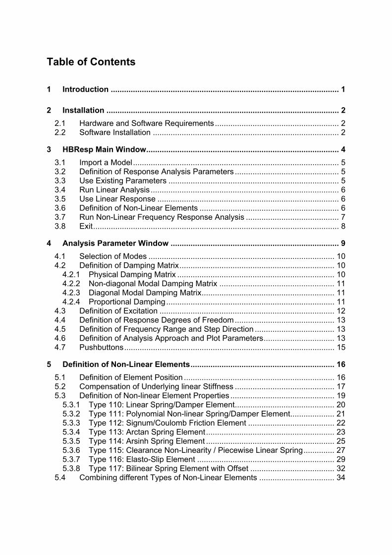
Table of Contents
1 Introduction ....................................................................................................... 1
2 Installation ......................................................................................................... 2
2.1 Hardware and Software Requirements........................................................ 2 2.2 Software Installation .................................................................................... 2
3 HBResp Main Window....................................................................................... 4
3.1 Import a Model............................................................................................. 5 3.2 Definition of Response Analysis Parameters ............................................... 5 3.3 Use Existing Parameters ............................................................................. 5 3.4 Run Linear Analysis ..................................................................................... 6 3.5 Use Linear Response .................................................................................. 6 3.6 Definition of Non-Linear Elements ............................................................... 6 3.7 Run Non-Linear Frequency Response Analysis .......................................... 7 3.8 Exit............................................................................................................... 8
4 Analysis Parameter Window ............................................................................ 9
4.1 Selection of Modes .................................................................................... 10 4.2 Definition of Damping Matrix...................................................................... 10
4.2.1 Physical Damping Matrix ....................................................................... 10 4.2.2 Non-diagonal Modal Damping Matrix .................................................... 11 4.2.3 Diagonal Modal Damping Matrix............................................................ 11 4.2.4 Proportional Damping............................................................................ 11
4.3 Definition of Excitation ............................................................................... 12 4.4 Definition of Response Degrees of Freedom............................................. 13 4.5 Definition of Frequency Range and Step Direction .................................... 13 4.6 Definition of Analysis Approach and Plot Parameters................................ 13 4.7 Pushbuttons............................................................................................... 15
5 Definition of Non-Linear Elements................................................................. 16
5.1 Definition of Element Position .................................................................... 16 5.2 Compensation of Underlying linear Stiffness ............................................. 17 5.3 Definition of Non-linear Element Properties ............................................... 19
5.3.1 Type 110: Linear Spring/Damper Element............................................. 20 5.3.2 Type 111: Polynomial Non-linear Spring/Damper Element.................... 21 5.3.3 Type 112: Signum/Coulomb Friction Element ....................................... 22 5.3.4 Type 113: Arctan Spring Element.......................................................... 23 5.3.5 Type 114: Arsinh Spring Element .......................................................... 25 5.3.6 Type 115: Clearance Non-Linearity / Piecewise Linear Spring.............. 27 5.3.7 Type 116: Elasto-Slip Element .............................................................. 29 5.3.8 Type 117: Bilinear Spring Element with Offset ...................................... 32
5.4 Combining different Types of Non-Linear Elements .................................. 34
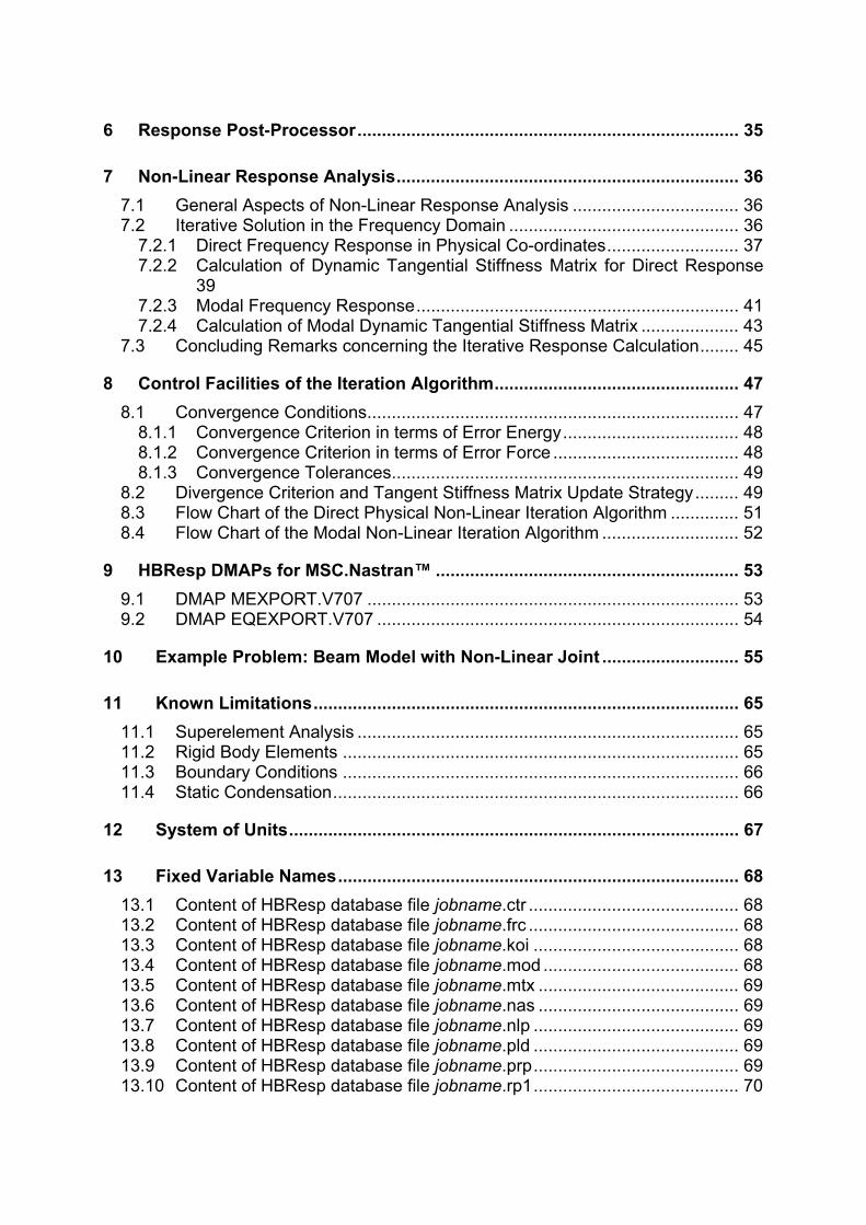
6 Response Post-Processor.............................................................................. 35
7 Non-Linear Response Analysis...................................................................... 36
7.1 General Aspects of Non-Linear Response Analysis .................................. 36 7.2 Iterative Solution in the Frequency Domain ............................................... 36
7.2.1 Direct Frequency Response in Physical Co-ordinates........................... 37 7.2.2 Calculation of Dynamic Tangential Stiffness Matrix for Direct Response 39 7.2.3 Modal Frequency Response.................................................................. 41 7.2.4 Calculation of Modal Dynamic Tangential Stiffness Matrix .................... 43
7.3 Concluding Remarks concerning the Iterative Response Calculation........ 45
8 Control Facilities of the Iteration Algorithm.................................................. 47
8.1 Convergence Conditions............................................................................ 47 8.1.1 Convergence Criterion in terms of Error Energy.................................... 48 8.1.2 Convergence Criterion in terms of Error Force ...................................... 48 8.1.3 Convergence Tolerances....................................................................... 49
8.2 Divergence Criterion and Tangent Stiffness Matrix Update Strategy......... 49 8.3 Flow Chart of the Direct Physical Non-Linear Iteration Algorithm .............. 51 8.4 Flow Chart of the Modal Non-Linear Iteration Algorithm ............................ 52
9 HBResp DMAPs for MSC.Nastran™ .............................................................. 53
9.1 DMAP MEXPORT.V707 ............................................................................ 53 9.2 DMAP EQEXPORT.V707 .......................................................................... 54
10 Example Problem: Beam Model with Non-Linear Joint ............................ 55
11 Known Limitations....................................................................................... 65
11.1 Superelement Analysis .............................................................................. 65 11.2 Rigid Body Elements ................................................................................. 65 11.3 Boundary Conditions ................................................................................. 66 11.4 Static Condensation................................................................................... 66
12 System of Units............................................................................................ 67
13 Fixed Variable Names.................................................................................. 68
13.1 Content of HBResp database file jobname.ctr ........................................... 68 13.2 Content of HBResp database file jobname.frc ........................................... 68 13.3 Content of HBResp database file jobname.koi .......................................... 68 13.4 Content of HBResp database file jobname.mod ........................................ 68 13.5 Content of HBResp database file jobname.mtx ......................................... 69 13.6 Content of HBResp database file jobname.nas ......................................... 69 13.7 Content of HBResp database file jobname.nlp .......................................... 69 13.8 Content of HBResp database file jobname.pld .......................................... 69 13.9 Content of HBResp database file jobname.prp.......................................... 69 13.10 Content of HBResp database file jobname.rp1.......................................... 70

13.11 Content of HBResp database file jobname.rp2.......................................... 70 13.12 Content of HBResp database file jobname.rp3.......................................... 70 13.13 Content of HBResp database file jobname.rp4.......................................... 70 13.14 Content of HBResp database file jobname.rp5.......................................... 70 13.15 Content of HBResp database file jobname.rp6.......................................... 71 13.16 Content of HBResp database file jobname.rp7.......................................... 71
14 Contact ......................................................................................................... 72
15 References ................................................................................................... 73

Introduction 1
1 Introduction HBResp is a software for non-linear frequency response analysis which uses the classical Harmonic Balance Method for the calculation of the frequency response of the fundamental harmonic of a non-linear structure. HBResp was designed under Mathworks MATLAB™ version 5.3 and is therefore platform independent. Essentially, the database for non-linear frequency response analysis consists of the system matrices of an MSC.Nastran™ FE model together with the mode shapes and eigenfrequencies. These data are provided by special HBResp DMAPs, which are included in the input deck for a standard Sol 103 analysis.
Figure 1: Typical Display of the Graphical User Interface of HBResp
HBResp allows the user to take into account concentrated structural non-linearities in a frequency response analysis, which are frequently observed at joints. The non-linear models currently supported include polynomial stiffness and damping non-linearities, signum/coulomb type friction non-linearity, clearance type non-linearities, elasto-slip non-linearities and bilinear springs. In addition, softening stiffness non-linearities with force deflection curves governed by the inverse tangent or the inverse hyperbolic sine function are included in HBResp, which overcome the drawbacks of non-linear softening polynomial springs.

Installation 2
2 Installation
2.1 Hardware and Software Requirements HBResp operates under Mathworks MATLAB™ Version 5.3, 6.0 and 6.51. Thus, an installation of Mathworks MATLAB™ is required to run HBResp and the hardware requirements for the MATLAB™ installation apply. The database for HBResp is provided by MSC.Nastran™ together with HBResp DMAPs. Therefore, an MSC.Nastran™ installation is required to provide the corresponding data,. This means, that in addition the hardware requirements for an MSC.Nastran™ installation have to be considered. For a proper display of the graphical user interface (GUI) a screen resolution of 1280x1024 or higher should be selected.
2.2 Software Installation Copy the 'hbresp' directory which includes all files and sub-directories from the installation CD to your hard disk drive. If the HBResp software was delivered as a zip file, then extract the zip file to a temporary directory of your hard disk drive. Subsequently move the ‘hbresp’ directory to the installation directory. Define the architecture of the machine that provides the MSC.Nastran™ output in the settings file 'hbset.m': %------------------------------------------------------------------------------- % architecture of machine (for MSC.Nastran op2/op4 reader): % 'n' - local machine format % 'l' - IEEE floating point with little-endian byte ordering % 'b' - IEEE floating point with big-endian byte ordering % 'd' - VAX D floating point and VAX ordering % 'g' - VAX G floating point and VAX ordering % 'c' - Cray floating point with big-endian byte ordering % 'a' - IEEE floating point with little-endian byte ordering and 64 bit long % data type % 's' - IEEE floating point with big-endian byte ordering and 64 bit long data % type %------------------------------------------------------------------------------- settings.arch = 'n';
A number of additional settings can be specified in this settings file, e.g. the figure sizes of the different GUIs and result windows (corrections might be needed in case of screen resolutions smaller than 1280x1024). The most important settings are those which are related to non-linear iteration algorithm (e.g. maximum number of iterations, convergence tolerances for non-linear iteration in terms of energy and force, control parameter for tangent stiffness matrix update). However, the default settings should only be altered in case of convergence problems of the non-linear iteration algorithm.
1 It should operate under higher MATLAB™ versions as well, but this has not been fully tested.

Installation 3
Finally add the HBResp path to your Mathworks MATLAB™ start-up file (usually: startup.m), e.g. add the HBResp pcode directory to the MATLAB™ path: Windows: path(path,'C:\hbresp\pcode'); Unix: path(path,'home/hbresp/pcode');
Getting Started / Main Window 4
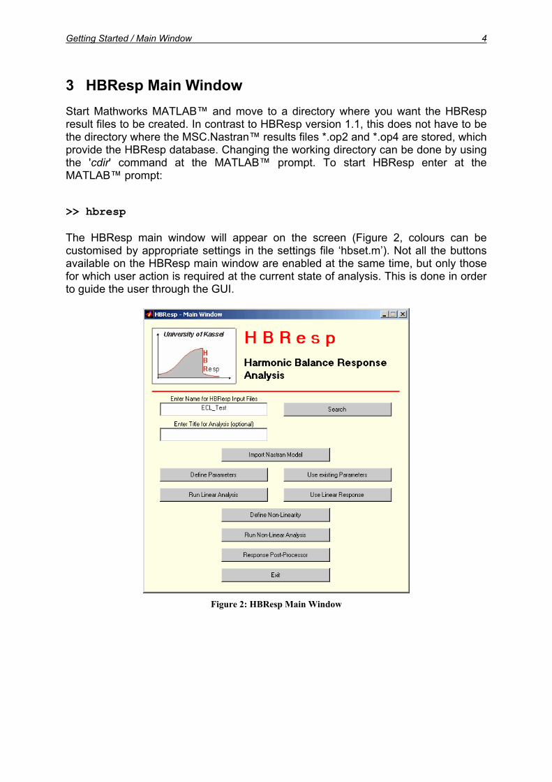
3 HBResp Main Window Start Mathworks MATLAB™ and move to a directory where you want the HBResp result files to be created. In contrast to HBResp version 1.1, this does not have to be the directory where the MSC.Nastran™ results files *.op2 and *.op4 are stored, which provide the HBResp database. Changing the working directory can be done by using the 'cdir' command at the MATLAB™ prompt. To start HBResp enter at the MATLAB™ prompt: >> hbresp The HBResp main window will appear on the screen ( , colours can be customised by appropriate settings in the settings file ‘hbset.m’). Not all the buttons available on the HBResp main window are enabled at the same time, but only those for which user action is required at the current state of analysis. This is done in order to guide the user through the GUI.
Figure 2
Figure 2: HBResp Main Window
Getting Started / Main Window 5
3.1 Import a Model From the HResp main window, MSC.Nastran™ finite element model data can be imported. This requires a jobname which is entered in the upper edit field 'Enter Name for HBResp Input Files'. An optional analysis title can be entered in the lower edit field 'Enter Title for Analysis (optional)'. In an analysis title was entered before the 'Import Nastran Model' pushbutton has been activated, it will appear at the beginning of the log file jobname.aus. After a jobname was entered, the MSC.Nastran™ data is imported by activating the 'Import Nastran Model' pushbutton. The user is then asked to select the corresponding MSC.Nastran™ *.op2 and *.op4 files. These files were created from a standard MSC.Nastran™ Sol 103 analysis with the HBResp DMAPs for exporting system matrices and data blocks included, see chapter 9 and chapter 10 for including the HBResp DMAPs. The MSC.Nastran™ data is loaded into the workspace and the HBResp database files jobname.mtx (system matrices), jobname.nas (displacement set information), jobname.pld (grid data) and jobname.mod (modal data) will be created in the current working directory, i.e. importing MSC.Nastran™ data via the ‘Import Nastran Model’ pushbutton involves a data translation from MSC.Nastran™ format into MATLAB™ based HBResp format. Once the MSC.Nastran™ data was imported and the corresponding HBResp database files were created, these files can directly be imported into HBResp by using the 'search' pushbutton. If this button is activated, the user is asked to select the corresponding jobname.mtx file. After the file selection, all the HBResp database files are loaded into the workspace, i.e. the data translation from MSC.Nastran™ format to HBResp format has only to be performed once.
3.2 Definition of Response Analysis Parameters After a model has been imported from either the MSC.Nastran™ files or from the HBResp database files, the frequency response analysis parameters can be specified by activating the 'Define Parameters' pushbutton. Frequency response analysis parameters consist of the active frequency range and the frequency resolution, the response and exciter degrees of freedom, damping, active mode shapes for modal frequency response, analysis approach (direct or modal), etc. For details of defining frequency response analysis parameters refer to chapter Analysis Parameter Window. The frequency response analysis parameters are read from the ‘Analysis Parameter Window’ and are stored in the HBResp database files jobname.ctr and jobname.frc.
3.3 Use Existing Parameters Once the frequency response parameters have been defined and the corresponding files jobname.ctr and jobname.frc are available, e.g. from a previous analysis, these files can directly be used by activating the button 'Use Parameters' on the HBResp main window (Figure 2). Activating this button will skip the definition of the frequency response analysis parameters.
Getting Started / Main Window 6
3.4 Run Linear Analysis After the frequency response analysis parameters were defined (either by using the 'Define Parameters' button or the 'Use Parameters' button), a linear frequency response analysis can be performed, which is initiated by activating the 'Run Linear Analysis' pushbutton. The output in terms of plotted response curves is dependent on the settings of the 'Plot Response' and 'Calculate and Plot Mode Indicator Function' checkboxes of the analysis parameter window (Figure 3). The results of the linear response analysis are stored in the current directory in the following HBResp result files: jobname.rp1: frequency domain mode indicator function jobname.rp2: real part of linear acceleration frequency response jobname.rp3: imaginary part of linear acceleration frequency response These files can be loaded into the MATLAB™ workspace (e.g. for post processing or detailed examination of the response) by using the load command. For example: >> load jobname.rp2 –mat The linear frequency response result files are a pre-requisite for the non-linear frequency response analysis, since the linear frequency response data is used for non-linear response estimation for the first response point of the non-linear response curve to be calculated. This involves that the ‘Run Non-Linear Analysis’ pushbutton gets only enabled as a linear response was calculated.
3.5 Use Linear Response If the linear frequency response result files are available, e.g. form a previous HBResp analysis, these result files can be used directly for non-linear frequency response estimation by activating the ‘Use Linear Response’ pushbutton on the HBResp main window. In this case, the linear response analysis is skipped and the existing jobname.rp1 to jobname.rp3 files will be used directly.
3.6 Definition of Non-Linear Elements Generally, non-linear elements are defined by activating the 'Define Non-Linearity' pushbutton on the HBResp main window. However, this pushbutton gets only enabled if the linear response data is available. If the 'Define Non-Linearity' pushbutton is activated, the user is asked to select a MATLAB™ m-file (ASCII file) containing the definition of non-linear elements in MATLAB™ format (element position defined by a matrix celas, element properties defined by a matrix pelas, compensation of underlying linear stiffness by variable compensation). For a proper definition of the non-linear elements, i.e. the content of the MATLAB™ m-file with the non-linear element definition, refer to the chapter Definition of Non-Linear Elements.
Getting Started / Main Window 7
The HBResp output file jobname.aus contains a listing of all non-linear elements defined in a non-linear frequency responses analysis. This listing should be reviewed by the user to ensure that all elements were properly defined.
3.7 Run Non-Linear Frequency Response Analysis After the non-linear elements were defined, the pushbutton 'Run Non-Linear Analysis' gets enabled and a non-linear frequency response analysis can be performed. The progress of the non-linear analysis is displayed on the status bar. If convergence problems are encountered such that the response at certain frequency points cannot be evaluated, the user is informed by corresponding messages on the MATLAB™ command window. After the non-linear analysis is finished, the results are stored in the current directory in the following files: jobname.rp4: real part of non-linear acceleration frequency response for
'Run-Up'. jobname.rp5: imaginary part of non-linear acceleration frequency response for
'Run-Up'. jobname.rp6: real part of non-linear acceleration frequency response for
'Run-Down'. jobname.rp7: imaginary part of non-linear acceleration frequency response for
'Run-Down'. The results of the non-linear responses analysis are plotted as non-linear accelerate frequency response curves. This is done automatically if the 'Plot Response' and 'Calculate and Plot Mode Indicator Function' checkboxes of the analysis parameter window ( ) have been activated. If these checkboxes were not activated, the response curves can be plotted by using the response postprocessor, see chapter
.
Figure 3
Response Post-Processor The HBResp result files of the non-linear response can be loaded to the MATLAB™ workspace by using the load command, e.g. to perform further post processing or for a detailed examination of the response curves: load jobname.rp4 –mat The most important variables for post processing are: fe excitation frequencies (vector of size [1,nf]), Ure real part of linear acceleration frequency response
(matrix of size [nresp,nf]), Uim imaginary part of linear acceleration frequency response
(matrix of size [nresp,nf]), Are_nl_u real part of non-linear acceleration frequency response for 'Run-Up'
(matrix of size [nresp,nf]), Aim_nl_u imaginary part of non-linear acceleration frequency response for
'Run-Up'(matrix of size [nresp,nf]), Are_nl_d real part of non-linear acceleration frequency response for 'Run-Down'
(matrix of size [nresp,nf]), Aim_nl_d imaginary part of non-linear acceleration frequency response for
'Run-Down' (matrix of size [nresp,nf]),

Getting Started / Main Window 8
where nresp is the number of response degrees of freedom and nf is the number of frequency points.
3.8 Exit By activating the 'Exit' pushbutton on the HBResp main window, all HBResp windows are closed. The output file jobname.aus (log file) holds information about the model data, the frequency response analysis parameters, the linear frequency response analysis, the non-linear elements and the non-linear frequency response analysis.

Analysis Parameter Window 9
4 Analysis Parameter Window After model data has been imported either from the MSC.Nastran™ result files (op2 and op4), or from the HBResp database files (*.mtx, *.mod, *.nas, *.pld), the frequency response analysis parameters can be specified by activating the 'Define Parameters' pushbutton on the HBResp main window (Figure 2). The frequency response analysis parameters comprise the upper and lower limit of the frequency range considered for analysis, the number of frequency points (frequency resolution), exciter degrees of freedom, excitation forces, response degrees of freedom, type of damping and damping values, modes to be considered for modal frequency response analysis, analysis approach, and settings for result postprocessing. From the ‘Analysis Parameter Window’ (see ) the frequency response parameters can be defined on a GUI. If all settings have been made, the analysis parameters are stored in the HBResp database files jobname.ctr and jobname.frc.
Figure 3

Analysis Parameter Window 10
Figure 3: HBResp Analysis Parameter Window
4.1 Selection of Modes In the upper left frame of the analysis parameter window, mode shapes can be selected. These mode shapes are used both, for modal transformation in case of a modal frequency response analysis and for the generation of a physical damping matrix in case of a direct frequency response analysis when diagonal modal damping matrix is selected for the type of damping. The mode shapes which are selected are the modes which were imported from the MSC.Nastran™ op2-file, i.e. the modes of the underlying linear system. In order to support the user when selecting the mode shapes, the corresponding eigenfrequencies and absolute mode numbers are displayed in the listbox for selecting the modes. The selection of the modes can either be done by mouse picking from the listbox (use the CTRL key for selecting multiple modes), or by entering the corresponding mode numbers into the edit field below the listbox (MATLAB™ format is required for all edit fields on the ‘Analysis Parameter Window’). If mode shapes are selected from the listbox, the edit field is automatically set to the corresponding values and vice versa. A check box allows for “adding” the eigenfrequencies of the selected mode shapes to the excitation frequencies used for frequency response analysis (only valid for linear analysis, because in non-linear analysis the eigenfrequencies are dependent on the excitation level).
4.2 Definition of Damping Matrix In the upper right frame of the ‘Analysis Parameter Window’ the type of damping can be defined and the corresponding damping values can be entered. The following different damping approaches are available:
• physical damping matrix , C• non-diagonal modal damping matrix , ∆• diagonal modal damping matrix ( )diag ξ , • proportional damping (Rayleigh damping), factor α for stiffness proportional
damping and factor β for mass proportional damping.
4.2.1 Physical Damping Matrix
If 'physical Damping Matrix' is the selected type of damping, the user has to enter the complete physical damping matrix in MATLAB™ format in the corresponding edit field. Since the number of values to be entered in the edit field becomes very large for an increasing number of model degrees of freedom, this type of damping is only recommended for relatively small systems. For example, the physical damping matrix of a 3 DOF system is entered in the following way:
[ ]11 12 13 21 22 23 31 32 33; ;C C C C C C C C C , where are the corresponding elements of the physical damping matrix . ijC C

Analysis Parameter Window 11
4.2.2 Non-diagonal Modal Damping Matrix If 'non-diagonal modal Damping Matrix' is the selected type of damping, the user has to enter the upper right triangle of the symmetric but non-diagonal modal damping matrix as a vector in MATLAB™ format. For example, the non-diagonal modal damping matrix of a system of arbitrary size, where only three modes are considered for modal transformation, is a 3-by-3 matrix. This symmetric 3-by-3 matrix may be entered as follows: [ ]11 12 13 22 23 33ξ ξ ξ ξ ξ ξ , where ijξ are the corresponding elements (in percent of critical damping) of the symmetric non-diagonal modal damping matrix and can be expressed as follows:
2
Ti j
iji j i j
ξµ µ ωω
=φ Cφ
,
with the modal masses iµ and jµ , and the (angular) eigenfrequencies iω and jω .
4.2.3 Diagonal Modal Damping Matrix If 'diagonal modal Damping Matrix' is the selected type of damping, the user has to enter the modal viscous damping ratios in percent of critical damping as a vector in MATLAB™ format. For example, if three modes are considered for a modal frequency response analysis three viscous modal damping ratios can be entered in the following way: [ ]11 22 33ξ ξ ξ , where ijξ are the viscous modal damping ratios in percent of critical damping of the three modes under consideration.
4.2.4 Proportional Damping In case of 'proportional Damping', the two factors for stiffness proportional damping and mass proportional damping have to be entered:
[ ]α β , where the physical damping matrix is expressed by the following equation:
α β= +C K M .
Analysis Parameter Window 12
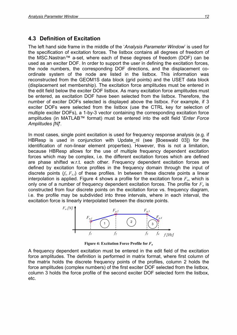
4.3 Definition of Excitation The left hand side frame in the middle of the ‘Analysis Parameter Window’ is used for the specification of excitation forces. The listbox contains all degrees of freedom of the MSC.Nastran™ a-set, where each of these degrees of freedom (DOF) can be used as an exciter DOF. In order to support the user in defining the excitation forces, the node numbers, the corresponding DOF directions, and the displacement co-ordinate system of the node are listed in the listbox. This information was reconstructed from the GEOM1S data block (grid points) and the USET data block (displacement set membership). The excitation force amplitudes must be entered in the edit field below the exciter DOF listbox. As many excitation force amplitudes must be entered, as excitation DOF have been selected from the listbox. Therefore, the number of exciter DOFs selected is displayed above the listbox. For example, if 3 exciter DOFs were selected from the listbox (use the CTRL key for selection of multiple exciter DOFs), a 1-by-3 vector containing the corresponding excitation force amplitudes (in MATLAB™ format) must be entered into the edit field 'Enter Force Amplitudes [N]'. In most cases, single point excitation is used for frequency response analysis (e.g. if HBResp is used in conjunction with Update_nl (see [Boeswald 03]) for the identification of non-linear element properties). However, this is not a limitation, because HBResp allows for the use of multiple frequency dependent excitation forces which may be complex, i.e. the different excitation forces which are defined are phase shifted w.r.t. each other. Frequency dependent excitation forces are defined by excitation force profiles in the frequency domain through the input of discrete points (fi, Fx,i) of these profiles. In between these discrete points a linear interpolation is applied. Figure 4 shows a profile for the excitation force Fa, which is only one of a number of frequency dependent excitation forces. The profile for Fa is constructed from four discrete points on the excitation force vs. frequency diagram, i.e. the profile may be subdivided into three intervals, where in each interval, the excitation force is linearly interpolated between the discrete points.
321
Fa,4
Fa,3Fa,2
Fa,1
f1
Fa [N]
f [Hz] f2 f3 f4
Figure 4: Excitation Force Profile for Fa
A frequency dependent excitation must be entered in the edit field of the excitation force amplitudes. The definition is performed in matrix format, where first column of the matrix holds the discrete frequency points of the profiles, column 2 holds the force amplitudes (complex numbers) of the first exciter DOF selected from the listbox, column 3 holds the force profile of the second exciter DOF selected form the listbox, etc.
Analysis Parameter Window 13
For example, the following matrix defines the excitation force profiles for the excitation forces Fa, Fb to Fx., where each profile is defined by n discrete points, i.e. n-1 intervals. Note the semicolons at the end of each row of the matrix and the brackets at the beginning of the first row and the end of the last row. [ f F F1 a,1 b,
f F F ... F ; 1 ... Fx,1;
2 a,2 b,2 x,2
... ... ... ... ... fn Fa,n Fb,n ... Fx,n ];
The excitation forces may be complex, i.e. a phase shift between two exciter forces can be taken into account. The real part as well as the imaginary part of the force vector is then linearly interpolated within a certain interval of the force profile.
4.4 Definition of Response Degrees of Freedom HBResp will calculate the acceleration frequency response for all degrees of freedom selected from the listbox in the right hand side frame in the middle of the ‘Analysis Parameter Window’. Again, the node numbers, the degree of freedom direction, and the displacement co-ordinate system are listed in order to give support in the selection of response degrees of freedom.
4.5 Definition of Frequency Range and Step Direction The lower left hand side frame of the ‘Analysis Parameter Window’ allows for the definition of the frequency axis used for frequency response analysis (lower frequency limit, upper frequency limit and number of frequency points). The step direction is only valid for non-linear response analysis. This feature may be interesting in cases of unstable responses of non-linear systems, because the response calculated for a 'Run-Up' will look different than that calculated for a 'Run-Down'. If the option 'Run-Up and Run-Down' is selected, the response will be calculated first for a 'Run-Up' and subsequently for a 'Run-Down'. Here, run-up means that the frequency response analysis starts at the lower frequency limit and steps towards the upper frequency limit, whereas run-down means that the frequency response analysis starts at the upper frequency limit and steps towards the lower frequency limit.
4.6 Definition of Analysis Approach and Plot Parameters The lower right hand side frame of the ‘Analysis Parameter Window’ allows for the definition of the analysis approach used for frequency response analysis. Either 'modal' or 'direct' approach can be selected. This parameter is only active for non-linear response analysis. The linear response analysis is always performed using the modal approach. When using the modal approach, the equation of motion is transformed to the modal domain and (in case of a non-linear analysis) the non-linear equilibrium iteration is performed on only a few modal (generalised) degrees of freedom. This is done at each frequency point of the response curve, where the number of generalised degrees of freedom is defined by the number of modes selected from the upper left hand side frame of the analysis parameter window. The modal frequency response
Analysis Parameter Window 14
algorithm is the recommended approach for large scale systems. This approach is efficient, even though a modal transformation and back-transformation have to be performed in each iteration step (back-transformation is necessary for the evaluation of the physical non-linear element matrices, which are dependent on the physical vibration amplitudes). The modal approach should always be used in conjunction with the ‘compensation flag’ for the compensation of the underlying linear stiffness of non-linear elements in order to avoid possible inaccuracies due to significant stiffness changes, see chapter . Compensation of Underlying linear Stiffness When using the direct approach, the equilibrium iteration at each frequency point of the response is performed directly using the physical degrees of freedom of the model, i.e. the MSC.Nastran™ a-set degrees of freedom. If a diagonal modal damping matrix is the selected type of damping and the direct approach is selected, the physical damping matrix is generated from an inverse modal transformation using the linear mode shapes imported form the MSC.Nastran™ op2 file. The direct approach is not recommended for large scale models, because convergence problems may occur if the number of degrees of freedom is too large. In addition, the amount memory needed to store the physical system matrices in the workspace may be significant. Details of the two frequency response analysis approaches mentioned above can be found in the chapter . Non-Linear Response Analysis In addition to the popup menu for the selection of the analysis approach, there are two checkboxes available for result plot control. If the first checkbox 'Plot Response after Analysis' is activated, the frequency response curves will be plotted just after they have been analysed (this checkbox has the same meaning as the variable plot_r of the jobname.un5 file of the non-linear parameter identification software Update_nl, see [Boeswald 03]). The second checkbox 'Calculate and Plot Mode Indicator Function' requests the calculation of the multivariate mode indicator function of the linear response. In any case, the results of the frequency response analysis are stored in several files in the current directory: jobname.rp1: frequency domain multivariate mode indicator function jobname.rp2: real part of linear acceleration frequency response jobname.rp3: imaginary part of linear acceleration frequency response jobname.rp4: real part of non-linear acceleration frequency response for
'Run-Up' jobname.rp5: imaginary part of non-linear acceleration frequency response for
'Run-Up' jobname.rp6: real part of non-linear acceleration frequency response for
'Run-Down' jobname.rp7: imaginary part of non-linear acceleration frequency response for
'Run-Down' These files can be loaded into the MATLAB™ workspace, e.g. by using the load command: load jobname.rp2 -mat

Analysis Parameter Window 15
The listbox 'Analysis Status Display Options' allows for the control of the amount of information displayed on the screen, or respectively, the amount of information which will be listed in the log file jobname.aus during analysis.
4.7 Pushbuttons There are three pushbuttons available at the bottom of the ‘Analysis Parameter Window’, these are the 'Create Input File', the 'Load Input File', and the 'Cancel' pushbutton. The ‘Create Input File’ pushbutton is used when all settings have been made by the user on the ‘Analysis Parameter Window’. Activating this pushbutton will cause the input made on this window to be stored in the HBResp database files jobname.frc (excitation force related parameters) and jobname.frc (all other parameters). The ‘Load Input File’ pushbutton may be used if the files jobname.frc and jobname.ctr are already available in the current directory, e.g. from a previous frequency response analysis. If this pushbutton is activated, the user is asked to select a *.ctr file. After selecting a file, the analysis parameters of the ‘Analysis Parameter Window’ are set according to the information stored the *.ctr and *.frc files selected by the user. After the information contained in these two files is restored on the ‘Analysis Parameter Window’, the user is allowed to alter these settings. If afterward the 'Create Input File' button is activated, the jobname.ctr and jobname.frc files will be created and already existing jobname.ctr and jobname.frc will be overwritten. If the 'Cancel' button is activated, the analysis parameter window is closed and the settings made on the ‘Analysis Parameter Window’ will be neglected.
Definition of Non-Linear Elements 16
5 Definition of Non-Linear Elements In this chapter, the definition of the different linear and non-linear elements currently supported by HBResp is discussed. In principle, the definition of the non-linear elements is performed using one MATLAB™ m-file, which must contain the two variables celas and pelas (and the optional variable compensation). The format of these two variables is similar to the format of the MSC.Nastran™ CELAS and PELAS bulk data cards.
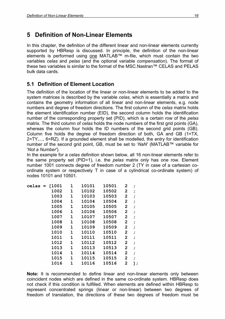
5.1 Definition of Element Location The definition of the location of the linear or non-linear elements to be added to the system matrices is described by the variable celas, which is essentially a matrix and contains the geometry information of all linear and non-linear elements, e.g. node numbers and degree of freedom directions. The first column of the celas matrix holds the element identification number (EID), the second column holds the identification number of the corresponding property set (PID), which is a certain row of the pelas matrix. The third column of celas holds the node numbers of the first grid points (GA), whereas the column four holds the ID numbers of the second grid points (GB). Column five holds the degree of freedom direction of both, GA and GB (1=TX, 2=TY,..., 6=RZ). If a grounded element shall be modelled, the entry for identification number of the second grid point, GB, must be set to ‘NaN’ (MATLAB™ variable for 'Not a Number'). In the example for a celas definition shown below, all 16 non-linear elements refer to the same property set (PID=1), i.e. the pelas matrix only has one row. Element number 1001 connects degree of freedom number 2 (TY in case of a cartesian co-ordinate system or respectively T in case of a cylindrical co-ordinate system) of nodes 10101 and 10501. celas = [1001 1 10101 10501 2 ; 1002 1 10102 10502 2 ; 1003 1 10103 10503 2 ; 1004 1 10104 10504 2 ; 1005 1 10105 10505 2 ; 1006 1 10106 10506 2 ; 1007 1 10107 10507 2 ; 1008 1 10108 10508 2 ; 1009 1 10109 10509 2 ; 1010 1 10110 10510 2 ; 1011 1 10111 10511 2 ; 1012 1 10112 10512 2 ; 1013 1 10113 10513 2 ; 1014 1 10114 10514 2 ; 1015 1 10115 10515 2 ; 1016 1 10116 10516 2 ]; Note: It is recommended to define linear and non-linear elements only between coincident nodes which are defined in the same co-ordinate system. HBResp does not check if this condition is fulfilled. When elements are defined within HBResp to represent concentrated springs (linear or non-linear) between two degrees of freedom of translation, the directions of these two degrees of freedom must be

Definition of Non-Linear Elements 17
coaxial. Even small deviations in direction can induce significant moment to the model that does not exist in the physical structure, see [Nastran 94]. Therefore, the HBResp elements are not suited for transmission of transverse loads between non-coincident nodes. This is illustrated in Figure 5.
Axial and Moment Load Transmission:
Non-Coincident Nodes are Valid
Transverse Load Transmission: Non-Coincident Nodes are Invalid
1u
1ϕ 2ϕ
2uGBGA1v 2v
GA GB
Figure 5: Connection of Nodes by Non-linear Elements
All elements which may be defined within HBResp are 2-degree of freedom elements. Thus, the element definition by the celas entry is the same for all types of linear and non-linear elements discussed below.
5.2 Compensation of Underlying linear Stiffness Different types of non-linear elements may be defined within HBResp, while all non-linear elements are characterised by different force deflection curves. For example,
shows the force deflection curves of three different types of non-linear elements, each with an underlying linear stiffness. The underlying linear stiffness is the slope of the force deflection curve at the origin of the force deflection diagram, i.e. the derivative of the restoring force of the non-linear element with respect to the relative displacement of the element degrees of freedom at zero relative displacement. Most of the non-linear elements available in HBResp have such an underlying linear stiffness.
Figure 6
Figure 6: Non-linear Elements with underlying linear Stiffness
Figure 6
Generally, non-linear elements defined in HBResp may be added to the existing system matrices, which were originally imported from MSC.Nastran™, or the non-linear elements can replace already existing linear elements in the system matrices. If non-linear elements, which have such an underlying linear stiffness as shown in
, are simply added to the system matrices, the modal properties of the underlying linear model would be influenced by the additional linear stiffness introduced by the underlying linear stiffness of the non-linear elements. In this case, a linear frequency response curve (without any non-linear element included) would have resonance peaks at different locations than the non-linear frequency response curve, which is evaluated for a very low excitation force level with almost zero vibration amplitudes. In most cases, however, it is desirable that the linear frequency response equals the non-linear frequency response for low excitation force levels,

Definition of Non-Linear Elements 18
which would not be the case if the non-linear elements are simply added to the structure. To overcome this problem, the compensation flag is introduced in HBResp version 1.2. By setting this compensation flag in the m-file with the definition of the non-linear element properties, the underlying linear stiffness of a non-linear element is determined and only the difference between the actual amplitude dependent non-linear stiffness and the underlying linear stiffness is added to the structure, i.e. for very low vibration levels, where the non-linearity is barely activated, the non-linear frequency response passes into the linear frequency response. The compensation flag is set, if the non-linear element definition file contains the following line: compensation = 1; By setting the variable compensation to “1”, already existing linear spring elements, which are contained in the stiffness matrix coming from MSC.Nastran™, will be replaced by non-linear elements having an amplitude dependent non-linear stiffness, but the same underlying linear stiffness as the linear spring elements which will be replaced. This is illustrated in Figure 7, where the restoring force of the linear spring and the restoring force of a non-linear spring are plotted together. It can be observed, that for small relative displacements, the linear and the non-linear restoring forces are identical. The variable compensation (compensation flag) is optional. Its default value is “0”, i.e. the non-linear elements will just be added to the system matrices. If the variable compensation is not contained in the m-file with the non-linear element definition, it will automatically be set to “0”.
Figure 7: Replacement of Linear Spring by Amplitude Dependent Non-Linear Spring

Definition of Non-Linear Elements 19
Note: If the compensation flag is used, it is up to the user to ensure that there really exists a linear spring stiffness in the stiffness matrix, which is replaced by an amplitude dependent non-linear stiffness whose underlying linear stiffness equals the linear spring stiffness to be replaced. If this is not the case, the compensation flag should not be set, because the substitution of a non-existing spring with a non-linear spring is physically not meaningful.
5.3 Definition of Non-linear Element Properties In the following, the different non-linear elements are described in the time domain by discussing their force deflection curves (restoring forces vs. relative displacement). By applying the Harmonic Balance Method the factor time is eliminated and the restoring force functions can be expressed as a function of the amplitude of the relative displacement between those degrees of freedom, where the element is located, i.e. the non-linear elements are transformed into equivalent springs and equivalent viscous dampers with vibration amplitude dependent properties. The Harmonic Balance Method is discussed extensively in [Worden 01]. Special information about the harmonic balance approach used in HBResp can be found in [Meyer 01]. Furthermore, special information about modelling flanged joints can be found in [Boeswald 02a]. In general, the variable pelas is a matrix, where each row of this matrix defines the properties of one type of non-linear element. The first two entries of each row of pelas are common for all types of non-linear elements. The last four entries, however, are element type dependent: pelas = [PID TYPE (4 element type dependent entries) ]; PID is the property set identification number which is referenced on a celas entry, and TYPE is the non-linear element type number. The definition of the properties of the different types of non-linear elements which are available in HBResp is discussed in the following chapters.
Definition of Non-Linear Elements 20
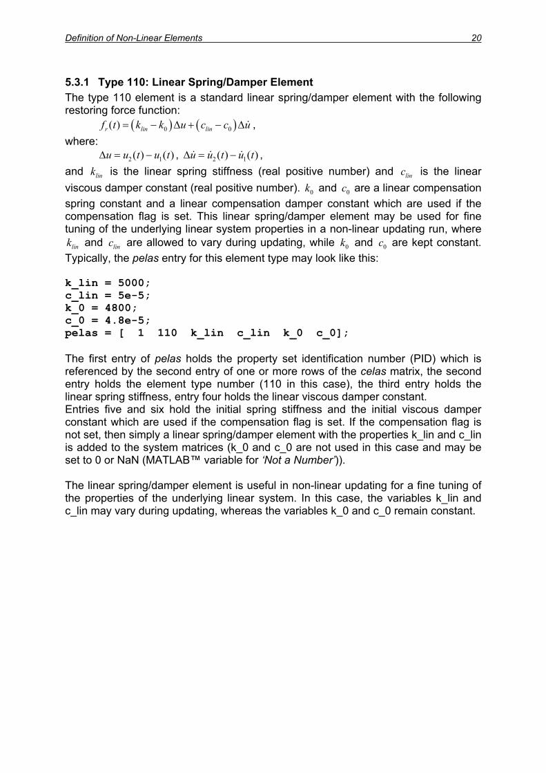
5.3.1 Type 110: Linear Spring/Damper Element The type 110 element is a standard linear spring/damper element with the following restoring force function: ( ) ( )0 0( )r lin linf t k k u c c= − ∆ + − ∆u , where: , ∆ = , 2 1( ) ( )u u t u t∆ = − 2 1( ) ( )u u t u t−and is the linear spring stiffness (real positive number) and is the linear viscous damper constant (real positive number). and are a linear compensation spring constant and a linear compensation damper constant which are used if the compensation flag is set. This linear spring/damper element may be used for fine tuning of the underlying linear system properties in a non-linear updating run, where
and are allowed to vary during updating, while and are kept constant. Typically, the pelas entry for this element type may look like this:
link linc
0k 0c
0klink linc 0c
k_lin = 5000; c_lin = 5e-5; k_0 = 4800; c_0 = 4.8e-5; pelas = [ 1 110 k_lin c_lin k_0 c_0]; The first entry of pelas holds the property set identification number (PID) which is referenced by the second entry of one or more rows of the celas matrix, the second entry holds the element type number (110 in this case), the third entry holds the linear spring stiffness, entry four holds the linear viscous damper constant. Entries five and six hold the initial spring stiffness and the initial viscous damper constant which are used if the compensation flag is set. If the compensation flag is not set, then simply a linear spring/damper element with the properties k_lin and c_lin is added to the system matrices (k_0 and c_0 are not used in this case and may be set to 0 or NaN (MATLAB™ variable for ‘Not a Number’)). The linear spring/damper element is useful in non-linear updating for a fine tuning of the properties of the underlying linear system. In this case, the variables k_lin and c_lin may vary during updating, whereas the variables k_0 and c_0 remain constant.
Definition of Non-Linear Elements 21
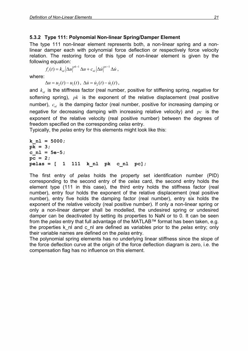
5.3.2 Type 111: Polynomial Non-linear Spring/Damper Element The type 111 non-linear element represents both, a non-linear spring and a non-linear damper each with polynomial force deflection or respectively force velocity relation. The restoring force of this type of non-linear element is given by the following equation: 1 1( ) pk pc
r nl nlf t k u u c u− −= ∆ ∆ + ∆ ∆u , where: , ∆ = , 2 1( ) ( )u u t u t∆ = − 2 1( ) ( )u u t u t−and is the stiffness factor (real number, positive for stiffening spring, negative for softening spring),
nlkpk is the exponent of the relative displacement (real positive
number), is the damping factor (real number, positive for increasing damping or negative for decreasing damping with increasing relative velocity) and
nlcpc is the
exponent of the relative velocity (real positive number) between the degrees of freedom specified on the corresponding celas entry. Typically, the pelas entry for this elements might look like this: k_nl = 5000; pk = 3; c_nl = 5e-5; pc = 2; pelas = [ 1 111 k_nl pk c_nl pc]; The first entry of pelas holds the property set identification number (PID) corresponding to the second entry of the celas card, the second entry holds the element type (111 in this case), the third entry holds the stiffness factor (real number), entry four holds the exponent of the relative displacement (real positive number), entry five holds the damping factor (real number), entry six holds the exponent of the relative velocity (real positive number). If only a non-linear spring or only a non-linear damper shall be modelled, the undesired spring or undesired damper can be deactivated by setting its properties to NaN or to 0. It can be seen from the pelas entry that full advantage of the MATLAB™ format has been taken, e.g. the properties k_nl and c_nl are defined as variables prior to the pelas entry; only their variable names are defined on the pelas entry. The polynomial spring elements has no underlying linear stiffness since the slope of the force deflection curve at the origin of the force deflection diagram is zero, i.e. the compensation flag has no influence on this element.
Definition of Non-Linear Elements 22
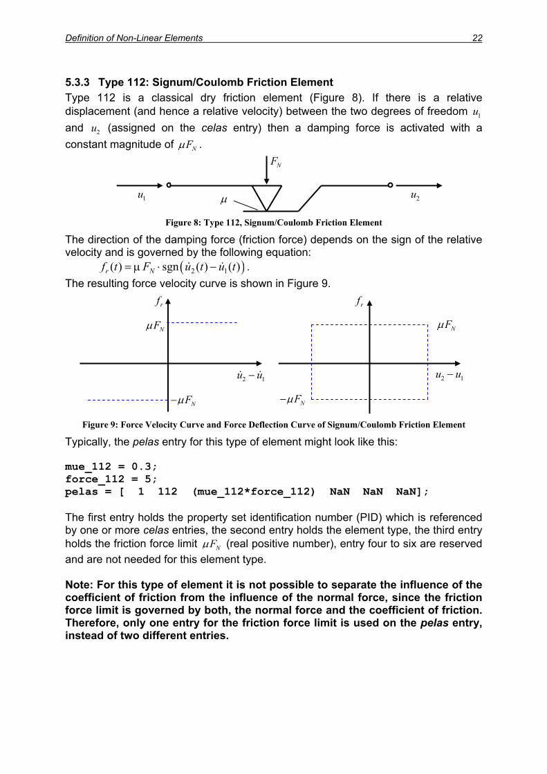
5.3.3 Type 112: Signum/Coulomb Friction Element Type 112 is a classical dry friction element (Figure 8). If there is a relative displacement (and hence a relative velocity) between the two degrees of freedom and (assigned on the celas entry) then a damping force is activated with a constant magnitude of
1u
2u
NFµ .
NF
µ1u 2u
Figure 8: Type 112, Signum/Coulomb Friction Element
The direction of the damping force (friction force) depends on the sign of the relative velocity and is governed by the following equation:
( )2 1( ) sgn ( ) ( )r Nf t F u t u t= µ ⋅ − . The resulting force velocity curve is shown in Figure 9.
rf
2 1u u−
NFµ
NFµ−NFµ−
NFµ
rf
2 1u u−
Figure 9: Force Velocity Curve and Force Deflection Curve of Signum/Coulomb Friction Element
Typically, the pelas entry for this type of element might look like this: mue_112 = 0.3; force_112 = 5; pelas = [ 1 112 (mue_112*force_112) NaN NaN NaN]; The first entry holds the property set identification number (PID) which is referenced by one or more celas entries, the second entry holds the element type, the third entry holds the friction force limit NFµ (real positive number), entry four to six are reserved and are not needed for this element type. Note: For this type of element it is not possible to separate the influence of the coefficient of friction from the influence of the normal force, since the friction force limit is governed by both, the normal force and the coefficient of friction. Therefore, only one entry for the friction force limit is used on the pelas entry, instead of two different entries.
Definition of Non-Linear Elements 23
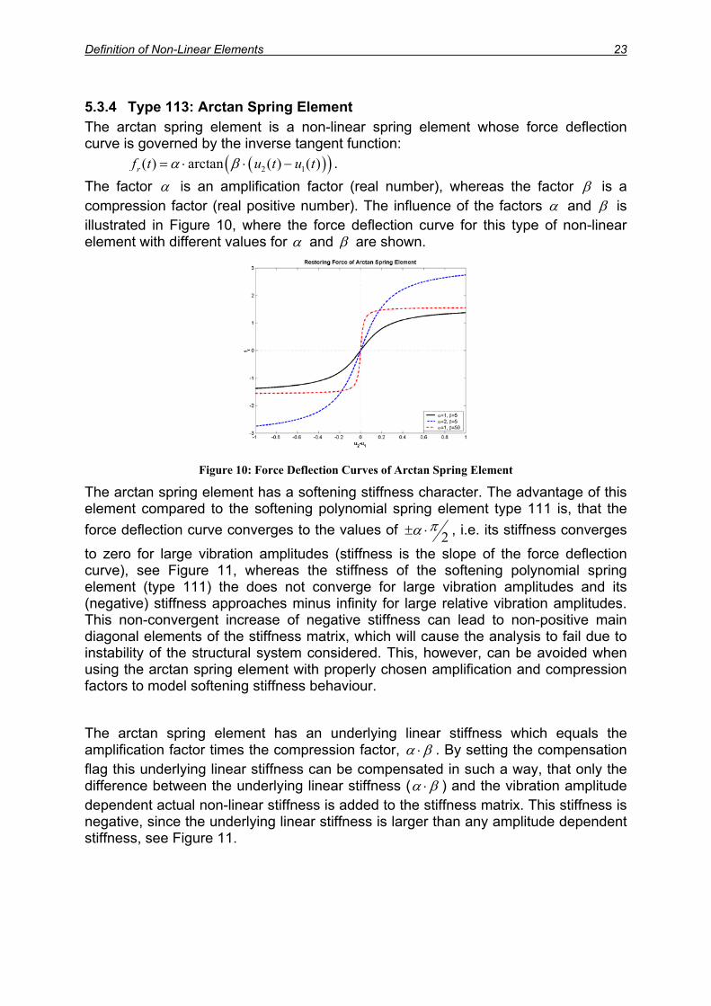
5.3.4 Type 113: Arctan Spring Element The arctan spring element is a non-linear spring element whose force deflection curve is governed by the inverse tangent function: ( )( )2 1( ) arctan ( ) ( )rf t u tα β= ⋅ ⋅ − u t . The factor α is an amplification factor (real number), whereas the factor β is a compression factor (real positive number). The influence of the factors α and β is illustrated in Figure 10, where the force deflection curve for this type of non-linear element with different values for α and β are shown.
Figure 10: Force Deflection Curves of Arctan Spring Element
The arctan spring element has a softening stiffness character. The advantage of this element compared to the softening polynomial spring element type 111 is, that the force deflection curve converges to the values of 2
πα± ⋅ , i.e. its stiffness converges
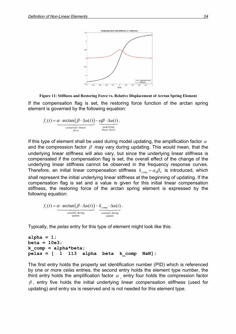
to zero for large vibration amplitudes (stiffness is the slope of the force deflection curve), see Figure 11, whereas the stiffness of the softening polynomial spring element (type 111) the does not converge for large vibration amplitudes and its (negative) stiffness approaches minus infinity for large relative vibration amplitudes. This non-convergent increase of negative stiffness can lead to non-positive main diagonal elements of the stiffness matrix, which will cause the analysis to fail due to instability of the structural system considered. This, however, can be avoided when using the arctan spring element with properly chosen amplification and compression factors to model softening stiffness behaviour. The arctan spring element has an underlying linear stiffness which equals the amplification factor times the compression factor, α β⋅ . By setting the compensation flag this underlying linear stiffness can be compensated in such a way, that only the difference between the underlying linear stiffness (α β⋅ ) and the vibration amplitude dependent actual non-linear stiffness is added to the stiffness matrix. This stiffness is negative, since the underlying linear stiffness is larger than any amplitude dependent stiffness, see Figure 11.
Definition of Non-Linear Elements 24
Figure 11: Stiffness and Restoring Force vs. Relative Displacement of Arctan Spring Element
If the compensation flag is set, the restoring force function of the arctan spring element is governed by the following equation: ( )( ) arctan ( ) ( )r
underlyingactual non linearlinear forceforce
f t u tα β αβ−
= ⋅ ⋅ ∆ − ⋅∆u t .
If this type of element shall be used during model updating, the amplification factor α and the compression factor β may vary during updating. This would mean, that the underlying linear stiffness will also vary, but since the underlying linear stiffness is compensated if the compensation flag is set, the overall effect of the change of the underlying linear stiffness cannot be observed in the frequency response curves. Therefore, an initial linear compensation stiffness 0 0compk α β= is introduced, which shall represent the initial underlying linear stiffness at the beginning of updating. If the compensation flag is set and a value is given for this initial linear compensation stiffness, the restoring force of the arctan spring element is expressed by the following equation: ( )( ) arctan ( ) ( )r c
variable during constant duringupdate update
ompf t u t kα β= ⋅ ⋅ ∆ − ⋅∆u t .
Typically, the pelas entry for this type of element might look like this: alpha = 1; beta = 10e3; k_comp = alpha*beta; pelas = [ 1 113 alpha beta k_comp NaN]; The first entry holds the property set identification number (PID) which is referenced by one or more celas entries, the second entry holds the element type number, the third entry holds the amplification factor α , entry four holds the compression factor β , entry five holds the initial underlying linear compensation stiffness (used for updating) and entry six is reserved and is not needed for this element type.
Definition of Non-Linear Elements 25
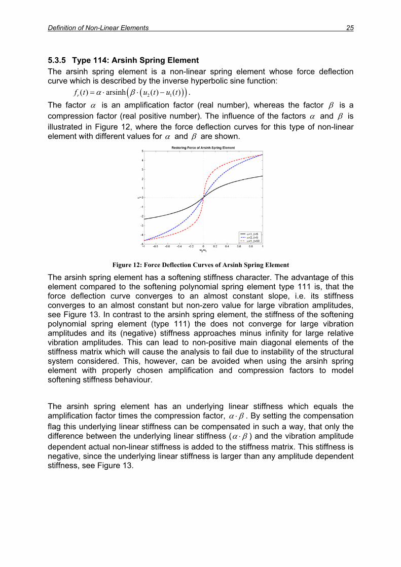
5.3.5 Type 114: Arsinh Spring Element The arsinh spring element is a non-linear spring element whose force deflection curve which is described by the inverse hyperbolic sine function: ( )( )2 1( ) arsinh ( ) ( )rf t u tα β= ⋅ ⋅ − u t . The factor α is an amplification factor (real number), whereas the factor β is a compression factor (real positive number). The influence of the factors α and β is illustrated in Figure 12, where the force deflection curves for this type of non-linear element with different values for α and β are shown.
Figure 12: Force Deflection Curves of Arsinh Spring Element
The arsinh spring element has a softening stiffness character. The advantage of this element compared to the softening polynomial spring element type 111 is, that the force deflection curve converges to an almost constant slope, i.e. its stiffness converges to an almost constant but non-zero value for large vibration amplitudes, see . In contrast to the arsinh spring element, the stiffness of the softening polynomial spring element (type 111) the does not converge for large vibration amplitudes and its (negative) stiffness approaches minus infinity for large relative vibration amplitudes. This can lead to non-positive main diagonal elements of the stiffness matrix which will cause the analysis to fail due to instability of the structural system considered. This, however, can be avoided when using the arsinh spring element with properly chosen amplification and compression factors to model softening stiffness behaviour.
Figure 13
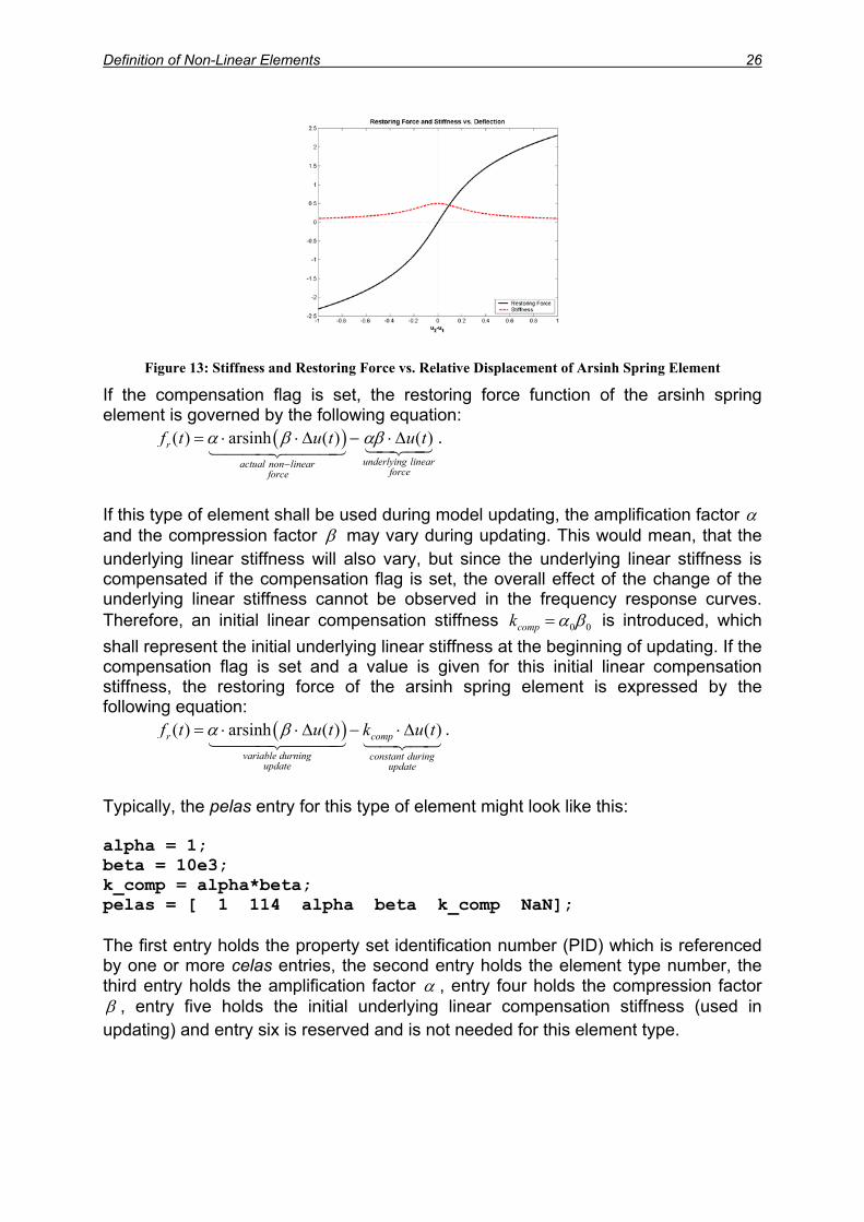
The arsinh spring element has an underlying linear stiffness which equals the amplification factor times the compression factor, α β⋅ . By setting the compensation flag this underlying linear stiffness can be compensated in such a way, that only the difference between the underlying linear stiffness (α β⋅ ) and the vibration amplitude dependent actual non-linear stiffness is added to the stiffness matrix. This stiffness is negative, since the underlying linear stiffness is larger than any amplitude dependent stiffness, see Figure 13.
Definition of Non-Linear Elements 26
Figure 13: Stiffness and Restoring Force vs. Relative Displacement of Arsinh Spring Element
If the compensation flag is set, the restoring force function of the arsinh spring element is governed by the following equation: ( )( ) arsinh ( ) ( )r
underlying linearactual non linearforceforce
f t u tα β αβ−
= ⋅ ⋅ ∆ − ⋅∆u t .
If this type of element shall be used during model updating, the amplification factor α and the compression factor β may vary during updating. This would mean, that the underlying linear stiffness will also vary, but since the underlying linear stiffness is compensated if the compensation flag is set, the overall effect of the change of the underlying linear stiffness cannot be observed in the frequency response curves. Therefore, an initial linear compensation stiffness 0 0compk α β= is introduced, which shall represent the initial underlying linear stiffness at the beginning of updating. If the compensation flag is set and a value is given for this initial linear compensation stiffness, the restoring force of the arsinh spring element is expressed by the following equation: ( )( ) arsinh ( ) ( )r c
variable durning constant duringupdate update
ompf t u t kα β= ⋅ ⋅ ∆ − ⋅∆u t .
Typically, the pelas entry for this type of element might look like this: alpha = 1; beta = 10e3; k_comp = alpha*beta; pelas = [ 1 114 alpha beta k_comp NaN]; The first entry holds the property set identification number (PID) which is referenced by one or more celas entries, the second entry holds the element type number, the third entry holds the amplification factor α , entry four holds the compression factor β , entry five holds the initial underlying linear compensation stiffness (used in updating) and entry six is reserved and is not needed for this element type.

Definition of Non-Linear Elements 27
5.3.6 Type 115: Clearance Non-Linearity / Piecewise Linear Spring With the type 115 non-linear element, a classical clearance type non-linearity can be modelled. The force deflection curve of this type of non-linear spring element is governed by the following equation:
( )
( ) ( )
( ) ( )
2 1 2 1
2 1 2 1
2 1 2 1
21
221
22
gapopened
gapr opened closed gap closed
gapopened closed gap closed
uk u u u u
uf k k u k u u u u
uk k u k u u u u
⋅ − ∀ − ≤
= − + − ∀ − >− − + − ∀ − < −
As can be seen from Figure 14 the stiffness of the clearance type non-linear spring element changes as the relative displacement ( 2 1u u )− exceeds the half gap length
gapu .
closed stiffness regime
gap
opened stiffness regime
Figure 14: Restoring Force vs. Relative Displacement of the Clearance Type Element
The underlying linear stiffness of the clearance type non-linear spring equals the opened gap stiffness k and may be compensated by setting the compensation flag, such that only the difference between the underlying linear stiffness and the actual vibration amplitude dependent non-linear stiffness is added to the stiffness matrix. In this case, the restoring force is governed by the following equation:
opened
( ) ( )
( ) ( )
2 1
2 1 2 1
2 1 2 1
0 2
22
22
gap
gap gapr closed opened
gap gapclosed opened
uu u
u uf k k u u u u
u uk k u u u u
∀ − ≤ = − ⋅ − − ∀ − >
− ⋅ − + ∀ − < −
.
If this type of element shall be used during model updating, the opened gap stiffness
, the closed gap stiffness k , and the gap length openedk closed gapu may be parameters and, thus, are allowed to vary. This would mean, that the underlying linear stiffness will also vary, but since the underlying linear stiffness is compensated when the compensation flag is set, the overall effect of the change of the underlying linear stiffness cannot be observed in the frequency response curves. Therefore, an initial

Definition of Non-Linear Elements 28
linear compensation stiffness ,0comp openedk k= is introduced, which shall represent the initial underlying linear stiffness at the beginning of updating. If the compensation flag is set and a value is given for this initial linear compensation stiffness, the restoring force of the clearance type spring element is expressed by the following equation:
( )
(
(
2 1
ap closed co
gap closed
u u
u k
u k
−
+
+
gap
compk
( )
( ) ) ( )
( ) ) ( )
2 1
2 1 2 1
2 1 2 1
21
221
22
gapopened comp
gapr opened closed g mp
gapopened closed comp
uk k u u
uf k k k u u u u
uk k k u u u u
− ⋅ ∀ − ≤
= − − ⋅ − ∀ − >− − − ⋅ − ∀ − < −
.
In this equation, k , , and opened closedk u are allowed to vary during updating, while the linear compensation stiffness remains constant. This allows for a fine tuning of the underlying linear stiffness. Typically, the pelas entry for this type of element might look like this: kopened = 5; kclosed = 5000; halfgap = 1e-4; k_comp = 5; pelas = [ 1 115 kopened kclosed halfgap k_comp ]; The first entry holds the property set identification number (PID) which is referened by one or more celas entries, the second entry holds the element type number, the third entry holds stiffness of the element when the gap is open (real number), entry four holds the stiffness of the element when the gap is closed (real number), entry five holds the half gap length (real positive number), whereas entry six holds the initial linear compensation stiffness which is used for model updating.
Definition of Non-Linear Elements 29
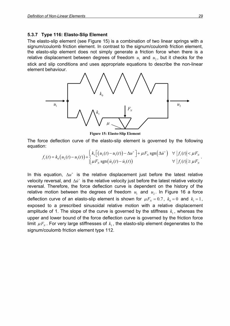
5.3.7 Type 116: Elasto-Slip Element The elasto-slip element (see Figure 15) is a combination of two linear springs with a signum/coulomb friction element. In contrast to the signum/coulomb friction element, the elasto-slip element does not simply generate a friction force when there is a relative displacement between degrees of freedom and u , but it checks for the stick and slip conditions and uses appropriate equations to describe the non-linear element behaviour.
1u 2
1u 2uNF
µ
1k
0k
Figure 15: Elasto-Slip Element
The force deflection curve of the elasto-slip element is governed by the following equation:
( )( ) ( )
( )1 2 1
0 2 12 1
( ) ( ) sgn ( )( ) ( ) ( )
sgn ( ) ( ) ( )N r
rN r
k u t u t u F u f t Ff t k u t u t
F u t u t f tN
NF
µ µ
µ µ
+ + − − ∆ + ∆ ∀ < = − + − ∀ ≥
.
In this equation, is the relative displacement just before the latest relative velocity reversal, and is the relative velocity just before the latest relative velocity reversal. Therefore, the force deflection curve is dependent on the history of the relative motion between the degrees of freedom u and . In Figure 16 a force deflection curve of an elasto-slip element is shown for
u+∆∆u+
1 2u
N 0.7Fµ = , and k0 0k = 1 1= , exposed to a prescribed sinusoidal relative motion with a relative displacement amplitude of 1. The slope of the curve is governed by the stiffness k , whereas the upper and lower bound of the force deflection curve is governed by the friction force limit
1
NFµ . For very large stiffnesses of , the elasto-slip element degenerates to the signum/coulomb friction element type 112.
1k
Definition of Non-Linear Elements 30
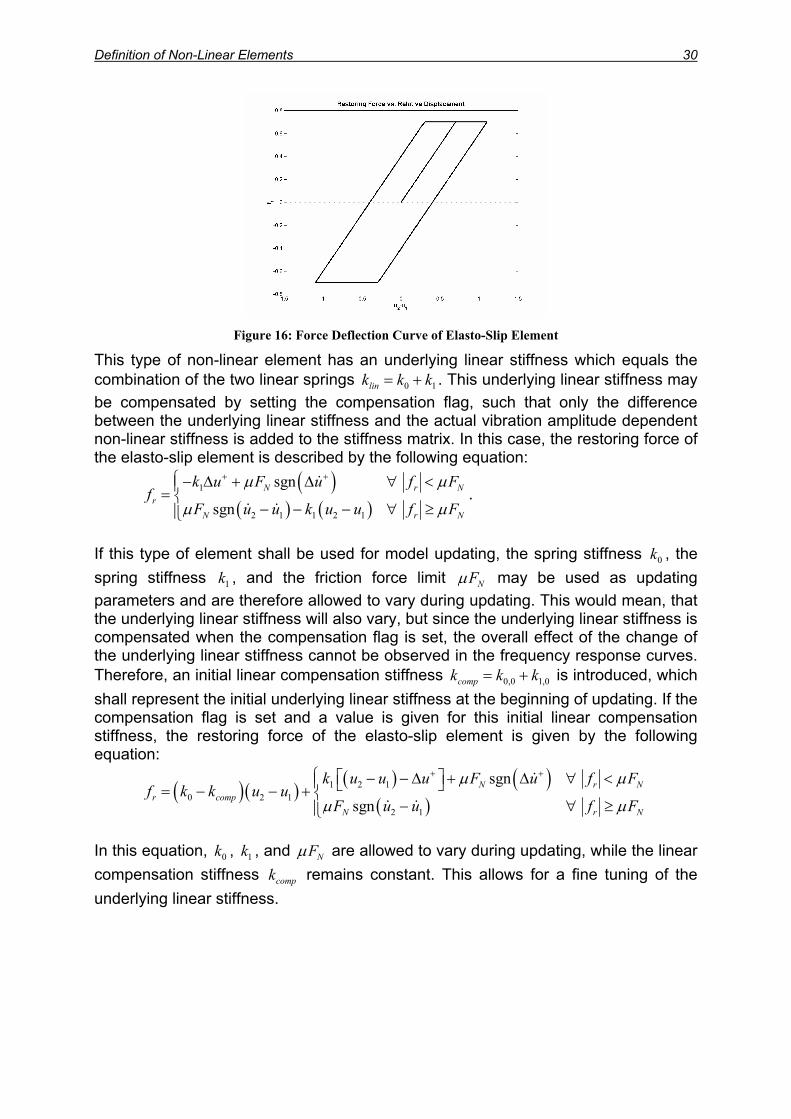
Figure 16: Force Deflection Curve of Elasto-Slip Element
This type of non-linear element has an underlying linear stiffness which equals the combination of the two linear springs k k0lin 1k= + . This underlying linear stiffness may be compensated by setting the compensation flag, such that only the difference between the underlying linear stiffness and the actual vibration amplitude dependent non-linear stiffness is added to the stiffness matrix. In this case, the restoring force of the elasto-slip element is described by the following equation:
( )
( ) ( )1
2 1 1 2 1
sgn
sgnN r
rN r
k u F u f Ff
F u u k u u fN
NF
µ µ
µ µ
+ +− ∆ + ∆ ∀ <= − − − ∀ ≥
.
If this type of element shall be used for model updating, the spring stiffness k , the spring stiffness , and the friction force limit
0
1k NFµ may be used as updating parameters and are therefore allowed to vary during updating. This would mean, that the underlying linear stiffness will also vary, but since the underlying linear stiffness is compensated when the compensation flag is set, the overall effect of the change of the underlying linear stiffness cannot be observed in the frequency response curves. Therefore, an initial linear compensation stiffness 0,0 1,0k kcomp k= + is introduced, which shall represent the initial underlying linear stiffness at the beginning of updating. If the compensation flag is set and a value is given for this initial linear compensation stiffness, the restoring force of the elasto-slip element is given by the following equation:
( )( )( ) ( )
( )1 2 1
0 2 12 1
sgn
sgnN r
r compN r
k u u u F u f Ff k k u u
F u u fN
NF
µ µ
µ µ
+ + − − ∆ + ∆ ∀ < = − − + − ∀ ≥
In this equation, , , and 0k 1k NFµ are allowed to vary during updating, while the linear compensation stiffness k remains constant. This allows for a fine tuning of the underlying linear stiffness.
comp

Definition of Non-Linear Elements 31
Typically, the pelas entry for the elasto-slip element might look like this: k0 = 0.5; k1 = 1.0 force = 0.7; k_comp = 1.5 pelas = [ 1 116 k1 force k0 k_comp ]; The first entry holds the property set identification number (PID) which is referenced by one or more celas entries, the second entry holds the element type number, the third entry holds the spring stiffness k . Entry four holds the friction force limit 1 NFµ , entry five holds the spring stiffness and entry six holds the initial underlying linear compensation stiffness k (used for updating).
0k
comp
Definition of Non-Linear Elements 32
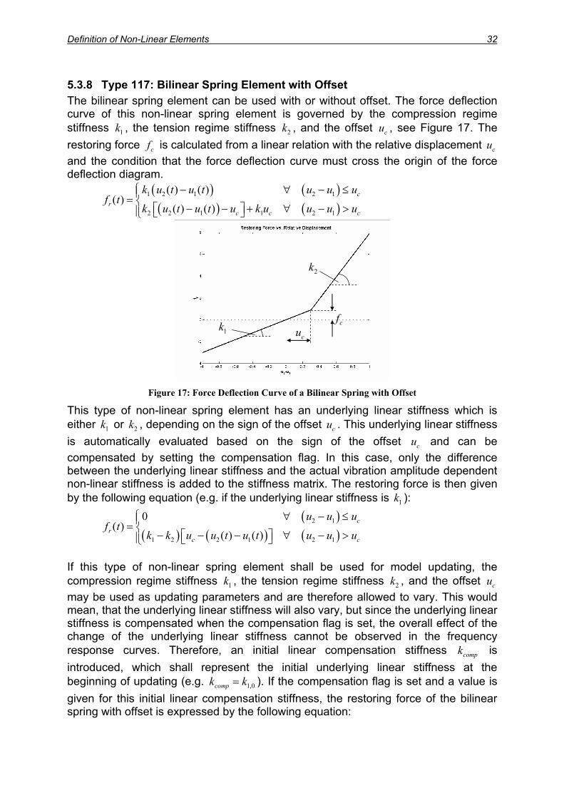
5.3.8 Type 117: Bilinear Spring Element with Offset The bilinear spring element can be used with or without offset. The force deflection curve of this non-linear spring element is governed by the compression regime stiffness , the tension regime stiffness , and the offset , see Figure 17. The restoring force
1k 2k cu
cf is calculated from a linear relation with the relative displacement u and the condition that the force deflection curve must cross the origin of the force deflection diagram.
c
( ) ( )( ) ( )
1 2 1 2 1
2 2 1 1 2 1
( ) ( )( )
( ) ( )c
rc c
k u t u t u u uf t
k u t u t u k u u u u
− ∀= − − + ∀ − > c
− ≤
2k
1kcu
cf
Figure 17: Force Deflection Curve of a Bilinear Spring with Offset
This type of non-linear spring element has an underlying linear stiffness which is either or k , depending on the sign of the offset . This underlying linear stiffness is automatically evaluated based on the sign of the offset and can be compensated by setting the compensation flag. In this case, only the difference between the underlying linear stiffness and the actual vibration amplitude dependent non-linear stiffness is added to the stiffness matrix. The restoring force is then given by the following equation (e.g. if the underlying linear stiffness is ):
1k 2 cu
cu
1k
( )
( ) ( ) ( )2 1
1 2 2 1 2 1
0( )
( ) ( )c
rc c
u u uf t
k k u u t u t u u u
∀ − ≤= − − − ∀ − >
If this type of non-linear spring element shall be used for model updating, the compression regime stiffness k , the tension regime stiffness , and the offset u may be used as updating parameters and are therefore allowed to vary. This would mean, that the underlying linear stiffness will also vary, but since the underlying linear stiffness is compensated when the compensation flag is set, the overall effect of the change of the underlying linear stiffness cannot be observed in the frequency response curves. Therefore, an initial linear compensation stiffness is introduced, which shall represent the initial underlying linear stiffness at the beginning of updating (e.g. k ). If the compensation flag is set and a value is given for this initial linear compensation stiffness, the restoring force of the bilinear spring with offset is expressed by the following equation:
1
comp
2k c
compk
1,0k=

Definition of Non-Linear Elements 33
( )( ) ( )( ) ( ) ( ) ( )
1 2 1 2 1
2 2 1 1 2 1
( ) ( )( )
( ) ( )
comp c
r
comp c comp c c
k k u t u t u u uf t
k k u t u t u k k u u u u
− − ∀ −= − − − + − ∀ −
≤
>.
In this equation, the compression regime stiffness k , the tension regime stiffness k , and the offset u are allowed to vary during updating, while the linear compensation stiffness remains constant. This allows for a fine tuning of the underlying linear stiffness.
1 2
c
compk
Typically, the pelas entry for this type of element might look like this: k1 = 50; k2 = 500; uc = 0.1; k_comp = 50; pelas = [ 1 117 k1 k2 uc k_comp ]; The first entry holds the property set identification number (PID) which is referenced by one or more celas entries, the second entry holds the element type number, the third entry holds the compression regime stiffness , entry four holds the stiffness of tension regime k , entry five holds the offset , and entry six holds the initial underlying linear compensation stiffness (used for updating).
1k
cu2
compk Note: The force deflection curve of this type of element cannot be described by an odd function. Generally, this will cause a response portion at 0 Hz, which is however not accounted for. Furthermore, if the offset is zero, the equivalent stiffness of the bilinear spring after harmonic balancing results in the average stiffness of and k , which is independent of both, frequency and amplitude, and makes a non-linear analysis not meaningful.
1k 2
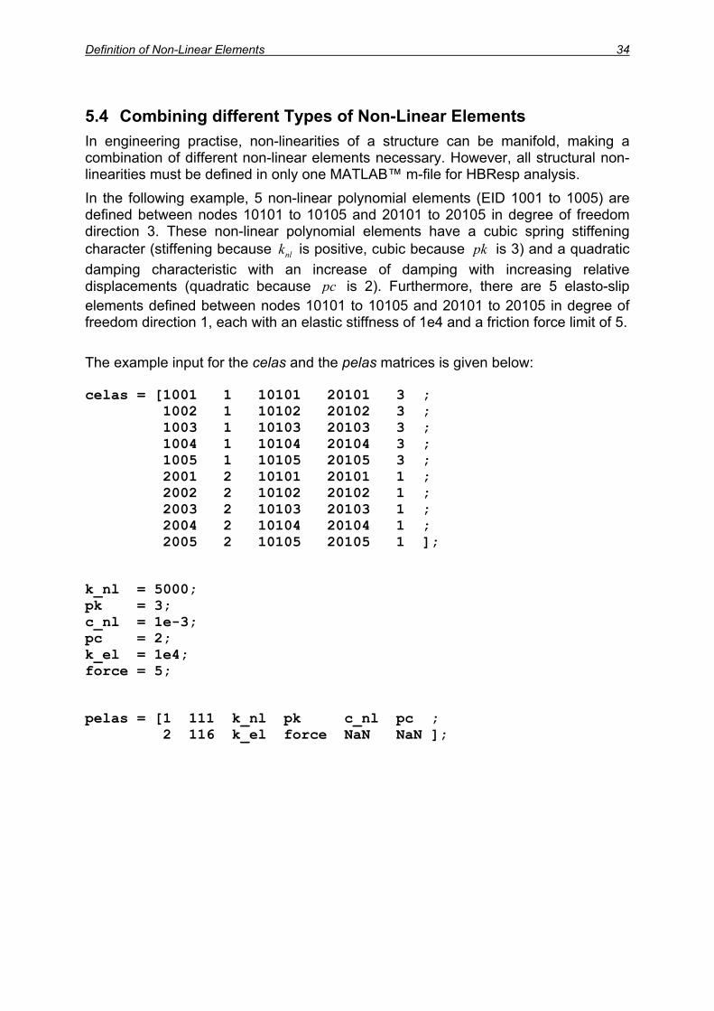
Definition of Non-Linear Elements 34
5.4 Combining different Types of Non-Linear Elements In engineering practise, non-linearities of a structure can be manifold, making a combination of different non-linear elements necessary. However, all structural non-linearities must be defined in only one MATLAB™ m-file for HBResp analysis. In the following example, 5 non-linear polynomial elements (EID 1001 to 1005) are defined between nodes 10101 to 10105 and 20101 to 20105 in degree of freedom direction 3. These non-linear polynomial elements have a cubic spring stiffening character (stiffening because k is positive, cubic because nl pk is 3) and a quadratic damping characteristic with an increase of damping with increasing relative displacements (quadratic because pc is 2). Furthermore, there are 5 elasto-slip elements defined between nodes 10101 to 10105 and 20101 to 20105 in degree of freedom direction 1, each with an elastic stiffness of 1e4 and a friction force limit of 5. The example input for the celas and the pelas matrices is given below: celas = [1001 1 10101 20101 3 ; 1002 1 10102 20102 3 ; 1003 1 10103 20103 3 ; 1004 1 10104 20104 3 ; 1005 1 10105 20105 3 ; 2001 2 10101 20101 1 ; 2002 2 10102 20102 1 ; 2003 2 10103 20103 1 ; 2004 2 10104 20104 1 ; 2005 2 10105 20105 1 ];
k_nl = 5000; pk = 3; c_nl = 1e-3; pc = 2; k_el = 1e4; force = 5;
pelas = [1 111 k_nl pk c_nl pc ; 2 116 k_el force NaN NaN ];
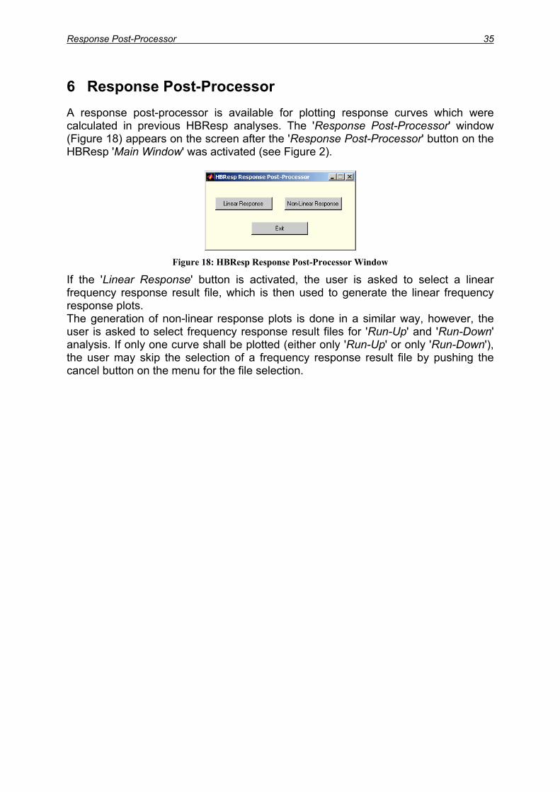
Response Post-Processor 35
6 Response Post-Processor A response post-processor is available for plotting response curves which were calculated in previous HBResp analyses. The 'Response Post-Processor' window (Figure 18) appears on the screen after the 'Response Post-Processor' button on the HBResp 'Main Window' was activated (see Figure 2).
Figure 18: HBResp Response Post-Processor Window
If the 'Linear Response' button is activated, the user is asked to select a linear frequency response result file, which is then used to generate the linear frequency response plots. The generation of non-linear response plots is done in a similar way, however, the user is asked to select frequency response result files for 'Run-Up' and 'Run-Down' analysis. If only one curve shall be plotted (either only 'Run-Up' or only 'Run-Down'), the user may skip the selection of a frequency response result file by pushing the cancel button on the menu for the file selection.
Non-Linear Response Analysis 36
7 Non-Linear Response Analysis
7.1 General Aspects of Non-Linear Response Analysis The calculation of the response of a non-linear system, both in the time domain and in the frequency domain, requires an iterative solution. The algorithms for non-linear time domain responses are well known and are a standard tool of most commercial finite element codes. In principle, the numerical integration schemes suitable for linear time domain response calculations are adopted for the non-linear time domain response algorithms, however, an iteration algorithm must be applied at each time step of the response in order to minimise the out-of-balance forces, which are a result of the dependency of the system matrices on the unknown response (which is the solution to the problem). Equation (1.1) shows the non-linear equation of motion in the time domain:
( ) ( ) ( ) ( ) ( ) ( )t t t+ + =M u C u u K u u f t
≠ 0
. (1.1)
The out-of-balance forces r(t) are calculated by putting the excitation force vector f(t) to the left hand side of the equation:
[ ]( ) ( ) ( ) ( ) ( ) ( ) ( ) ( ) ( )int t t t t t t− + + = − =f M u C u u K u u f f r . (1.2)
In this equation, the out-of-balance forces are calculated from the difference between the internal forces fin of the elements (reaction forces due to response) and the externally applied loads. If the structure is in the state of equilibrium, the out-of-balance force vector r(t) becomes zero. Thus, the non-linear equation (1.2) has to be solved iteratively, until the out-of-balance force vector r(t) is approximately zero. Often, this is achieved by applying either the classical Newton-Raphson iteration scheme, or by applying a line search algorithm, e.g. the BFGS method. The choice of the iteration scheme depends on the type of non-linearity present in the structure (large displacements but small strains, large displacements and large strains, material non-linearity, contact, etc.), see [Bathe 96].
7.2 Iterative Solution in the Frequency Domain The non-linear frequency response may be calculated either directly in physical displacement co-ordinates, or in modal co-ordinates by applying a modal transformation to the equation of motion using the modal matrix of the underlying linear system and perform the iterative calculation in a set of modal co-ordinates. Algorithms for direct and modal frequency responses are available in HBResp, however, both algorithms have advantages/drawbacks and are therefore presented in the following chapters.

Non-Linear Response Analysis 37
7.2.1 Direct Frequency Response in Physical Co-ordinates The iterative calculation of the non-linear frequency domain response starts from the equation of motion (already transformed to the frequency domain):
2 ˆ( ) ( ) ( ) ( , , ) ( ) ( )j −Ω + Ω + Ω = Ω Ω = Ω M C u K u u K u u u f , (1.3)
where is the excitation frequency. C u is the effective viscous damping matrix calculated by harmonic balancing using the actual velocity response u .
Ω ( )
Note: Generally, after applying the Harmonic Balance Method, the non-linearities are no longer dependent on the time history of the actual relative displacement response or the actual relative velocity response, but rather on the amplitude of the displacement response or the velocity response. However, in the following, this dependency of the matrices C and K is written in a more general form. When separating the linear part from the non-linear part, the damping matrix can be expressed as:
( ) ( )lin nl= +C u C C u . (1.4)
( )K u is the displacement dependent effective non-linear stiffness matrix calculated by harmonic balancing using the actual displacement response . Separating the linear part from the non-linear part yields:
u
( ) ( )lin nl= +K u K K u . (1.5)
The matrix represents the complex frequency and response dependent non-linear dynamic stiffness matrix.
ˆ ( , , )ΩK u u
The out-of-balance force vector in the frequency domain is calculated by bringing the excitation force vector f to the left hand side of the frequency domain equation of motion:
( )Ω
ˆ( ) ( , , ) ( ) ( , , ) ( ) ( )inΩ − Ω = Ω − Ω Ω = Ω ≠f f u u f K u u u r 0 . (1.6)
In analogy to the time domain, the out-of-balance forces in the frequency domain are calculated from the difference between the internal forces of the elements and the externally applied loads. If the structure is in the state of equilibrium the out-of-balance force vector r(Ω) becomes zero. However, for an arbitrary response vector the out-of-balance force vector ( )Ωr is generally non-zero due to the response dependency of the complex dynamic stiffness matrix at each frequency point Ω . Therefore, the out-of-balance force vector has to be minimised iteratively. In the HBResp response algorithm presented below, a modified Newton-Raphson scheme is used for this task. Assuming that the displacement response u is known at some past frequency points, e.g. , 1 1i i− −Ω → u 2i 2i− −Ω → u and 3i 3i− −Ω → u
iu
, then the response at the actual frequency point Ω is estimated by extrapolating the response curve from the past
frequency points to the actual frequency point Ω → . The superscript 0 denotes the 0-th iteration step in the calculation of . The type of extrapolation used depends on the number of response points available for extrapolation, e.g. polynomial extrapolation of third order if at least 4 response points are available, second order
i0
i ui

Non-Linear Response Analysis 38
extrapolation in case of 3 response points, and a linear extrapolation in case of 2 available response points. 0
1i i−= u
(nl ΩC u
0iK
1( , , )
−Ω u u
u
u is used in case that only one response point is available, e.g. at the beginning of the response analysis. At the first frequency point of the response curve, where the first non-linear response point has to be calculated, the corresponding linear response is used for the estimation of the non-linear response. However, this response estimation approach assumes that the frequency band of the non-linear response analysis starts with a frequency point, for which the difference between linear and non-linear response are negligible, i.e. the non-linear frequency response analysis should start with a frequency point located far away from a resonance peak.
0
ˆ
i=
=u u
The estimated initial non-linear response at frequency point Ω is then used to estimate the response dependent stiffness and damping matrices:
0iu i
0 0 (i i lin nl→ = +u K K K u0 )i
0 )ij
0 0i
0i
u
, (1.7)
0 0 0i i i linj= Ω → = +u u C C . (1.8)
From equation (1.8), it can be seen that the non-linear damping matrix Cnl depends on the displacement response, instead of the velocity response, since the velocity response is expressed in terms of displacement response pre-multiplied by . With the non-linear stiffness and damping matrices together with the (linear and constant) mass matrix, the non-linear dynamic stiffness matrix can be generated:
jΩ
0 2 0ˆi i i ij= −Ω + Ω +K M C , (1.9)
which is then used to calculate the out-of-balance forces at the 0-th iteration step from the difference of the vector of externally applied loads and the vector of internal forces (the index i of the vector of externally applied loads, fi, is used here to describe its frequency dependence):
0 ˆi i i= −r f K u . (1.10)
With the out-of-balance force vector , a better estimation of the true response u0ir i is
calculated by incrementing the response estimation by the incremental response
, which is caused by the out-of-balance forces :
0iu
00i∆u ir
1 0 0 0 0ˆi i i i t= + ∆ = + u u u u K r . (1.11)
The superscript 1 denotes the 1st iteration step in calculating the true response u . In
this equation, is the so called dynamic tangential stiffness matrix, which is the derivative of the vector of internal forces with respect to the actual displacement response vector :
i0ˆ ( , , )t ΩK u
0
0( , , )( , , )ˆ ( , , )
i
int
=
∂ Ω∂ Ω Ω =∂ ∂
u u
K u u uf u uK u uu u
. (1.12)
The calculation of the dynamic tangential stiffness matrix is one of the fundamental operations in an iteration algorithm and is typically expensive in terms of CPU time. Therefore, the next chapter is dedicated to the calculation of this matrix.

Non-Linear Response Analysis 39
Equation (1.11) again only yields an estimation of the true displacement response vector ui, since:
0 0ˆ ( , , )i t= Ω ∆r K u u u0i , (1.13)
assumes that a linear relation exists between the incremental response ∆ and the
out-of-balance loads , which is ,however, a non-linear relation.
0iu
0ir
With of equation (1.11) being a better estimation of the true displacement
response than u , the non-linear damping and stiffness matrices are evaluated again and a new non-linear dynamic stiffness matrix can be generated according to equation (1.9). This new non-linear dynamic stiffness matrix is then used to re-calculate the out-of-balance forces of the actual iteration step using equation (1.10), etc., etc. Altogether, equations (1.3) to (1.12) form the Newton-Raphson scheme for non-linear response analysis in the frequency domain.
1iu
iu 0i
7.2.2 Calculation of Dynamic Tangential Stiffness Matrix for Direct Response The dynamic tangent stiffness matrix for the direct physical response is the derivative of the vector of internal forces with respect to a given displacement response vector u0:
0
( , , )ˆ ( , , ) int
=
∂ ΩΩ =
∂ u u
f u uK u uu
. (1.14)
It should be noted, that the vector of internal forces is a function of both, the displacement response and the velocity response, however, in the frequency domain velocities can be expressed in terms of displacements by pre-multiplying with jΩ (a derivation with respect to time in the time domain corresponds to a pre-multiplication with jΩ in the frequency domain). Therefore, the velocity and displacement dependent vector of internal forces can be expressed as a displacement dependent quantity only. The vector of internal forces in the frequency domain is a superposition of the linear inertia forces, the linear restoring forces and damping forces, and of the non-linear restoring forces and damping forces:
, ,
2
( ) ( , , )
( , , ) ( ) ( )
( , , ) ( ) ( )lin in nl in
in lin lin nl nl
in lin lin nl nlj j jΩ Ω
Ω = + + + +
Ω = −Ω + Ω + + Ω Ω +f f
f u u M u C u K u C u u K u u
f u u M u C u K u C u u K uu u
u . (1.15)
The linear portion of the internal force vector is independent of the unknown response and its derivative with respect to the response vector yields the complex linear dynamic stiffness matrix ˆ ( )lin ΩK :
, 2( ) ˆ ( )lin inlin lin linj
∂ Ω= −Ω + Ω + = Ω
∂f
M C K Ku
. (1.16)
This matrix only has to be evaluated once for each frequency point Ω of the response curve. The derivative with respect to the displacement response of the non-linear portion of the internal force vector is evaluated directly by using a finite differences approach. In the first step, the vector of non-linear internal forces is evaluated for the actual displacement response vector u
i
0:
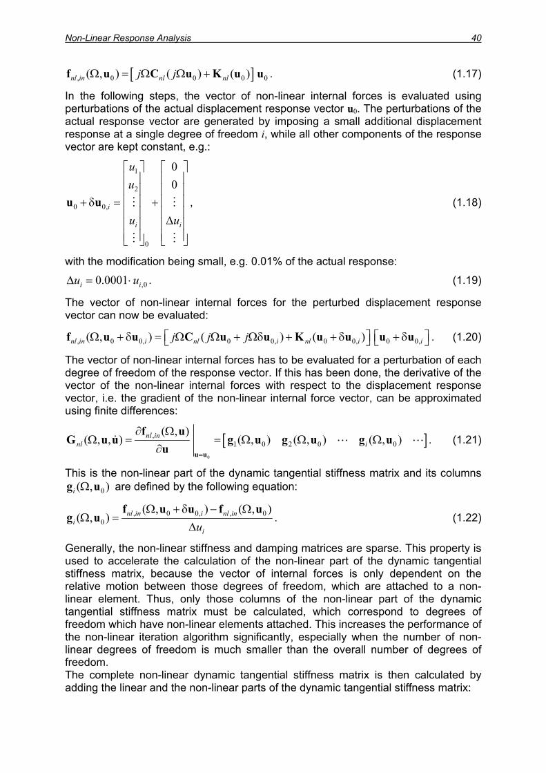
Non-Linear Response Analysis 40
[, 0 0 0( , ) ( ) ( )nl in nl nlj jΩ = Ω Ω +f u C u K u ] 0u . (1.17)
In the following steps, the vector of non-linear internal forces is evaluated using perturbations of the actual displacement response vector u0. The perturbations of the actual response vector are generated by imposing a small additional displacement response at a single degree of freedom i, while all other components of the response vector are kept constant, e.g.:
1
2
0 0,
0
00
i
i i
uu
u u
+ δ = + ∆
u u
iu
, (1.18)
with the modification being small, e.g. 0.01% of the actual response:
,00.0001iu∆ = ⋅ . (1.19)
The vector of non-linear internal forces for the perturbed displacement response vector can now be evaluated:
, 0 0, 0 0, 0 0, 0 0,( , ) ( ) ( )nl in i nl i nl i ij j j Ω + δ = Ω Ω + Ωδ + + δ + δ f u u C u u K u u u u . (1.20)
The vector of non-linear internal forces has to be evaluated for a perturbation of each degree of freedom of the response vector. If this has been done, the derivative of the vector of the non-linear internal forces with respect to the displacement response vector, i.e. the gradient of the non-linear internal force vector, can be approximated using finite differences:
[ ]0
,1 0 2 0 0
( , )( , , ) ( , ) ( , ) ( , )nl in
nl i=
∂ ΩΩ = = Ω Ω Ω
∂ u u
f uG u u g u g u g u
u. (1.21)
This is the non-linear part of the dynamic tangential stiffness matrix and its columns are defined by the following equation: 0( , )i Ωg u
, 0 0, ,0
( , ) ( , )( , ) nl in i nl in
iiu
Ω + δ − ΩΩ =
∆f u u f u
g u 0 . (1.22)
Generally, the non-linear stiffness and damping matrices are sparse. This property is used to accelerate the calculation of the non-linear part of the dynamic tangential stiffness matrix, because the vector of internal forces is only dependent on the relative motion between those degrees of freedom, which are attached to a non-linear element. Thus, only those columns of the non-linear part of the dynamic tangential stiffness matrix must be calculated, which correspond to degrees of freedom which have non-linear elements attached. This increases the performance of the non-linear iteration algorithm significantly, especially when the number of non-linear degrees of freedom is much smaller than the overall number of degrees of freedom. The complete non-linear dynamic tangential stiffness matrix is then calculated by adding the linear and the non-linear parts of the dynamic tangential stiffness matrix:
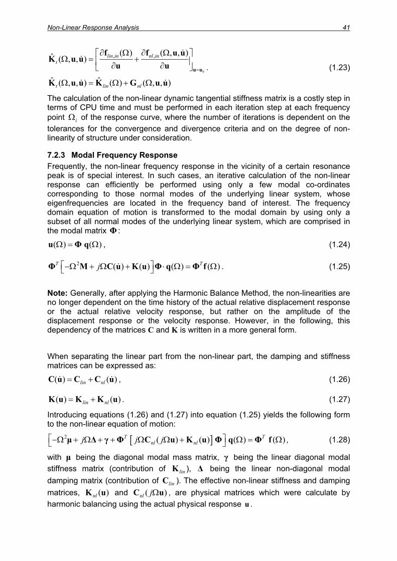
Non-Linear Response Analysis 41
0
, ,( ) ( , , )ˆ ( , , )
ˆ ˆ( , , ) ( ) ( , , )
lin in nl int
t lin nl
=
∂ Ω ∂ Ω Ω = + ∂ ∂
Ω = Ω + Ω
u u
f f u uK u u
u u
K u u K G u u
T
. (1.23)
The calculation of the non-linear dynamic tangential stiffness matrix is a costly step in terms of CPU time and must be performed in each iteration step at each frequency point of the response curve, where the number of iterations is dependent on the tolerances for the convergence and divergence criteria and on the degree of non-linearity of structure under consideration.
iΩ
7.2.3 Modal Frequency Response Frequently, the non-linear frequency response in the vicinity of a certain resonance peak is of special interest. In such cases, an iterative calculation of the non-linear response can efficiently be performed using only a few modal co-ordinates corresponding to those normal modes of the underlying linear system, whose eigenfrequencies are located in the frequency band of interest. The frequency domain equation of motion is transformed to the modal domain by using only a subset of all normal modes of the underlying linear system, which are comprised in the modal matrix : Φ
( ) ( )Ω = Ωu Φ q , (1.24)
2 ( ) ( ) ( ) ( )T j −Ω + Ω + ⋅ Ω = Ω Φ M C u K u Φ q Φ f . (1.25)
Note: Generally, after applying the Harmonic Balance Method, the non-linearities are no longer dependent on the time history of the actual relative displacement response or the actual relative velocity response, but rather on the amplitude of the displacement response or the velocity response. However, in the following, this dependency of the matrices C and K is written in a more general form. When separating the linear part from the non-linear part, the damping and stiffness matrices can be expressed as:
( ) ( )lin nl= +C u C C u , (1.26)
( ) ( )lin nl= +K u K K u . (1.27)
Introducing equations (1.26) and (1.27) into equation (1.25) yields the following form to the non-linear equation of motion:
[ ]2 ( ) ( ) ( ) ( )T Tnl nlj j j −Ω + Ω + + Ω Ω + Ω = Ω µ ∆ γ Φ C u K u Φ q Φ f , (1.28)
with µ being the diagonal modal mass matrix, being the linear diagonal modal stiffness matrix (contribution of K ), being the linear non-diagonal modal damping matrix (contribution of ). The effective non-linear stiffness and damping matrices, and C , are physical matrices which were calculate by harmonic balancing using the actual physical response .
γlin
lin
)u
∆C
( )nlK u (nl jΩu

Non-Linear Response Analysis 42
The matrices and in equation (1.28) are generally non-diagonal matrices, such that the modal equations of motion will always be coupled by the non-linear elements. Since only a limited number of modes need to be considered for modal response analysis, the order of the non-linear modal domain equation of motion is generally small, which increases the numerical efficiency dramatically, even though the equations are coupled.
Tnl nl=∆ Φ C Φ T
nl nl=γ Φ K Φ
After introducing the complex modal dynamic stiffness matrix:
[ ]2ˆ ( , , ) ( ) ( )Tnl nlj j jΩ = −Ω + Ω + + Ω Ω +Q u u µ ∆ γ Φ C u K u Φ , (1.29)
the non-linear equation of motion (1.28) can be written in the following form:
ˆ ( , , ) ( )TΩ =Q u u q Φ f Ω
0
2i− 3i
. (1.30)
The modal out-of-balance force vector z is then calculated from the difference between the modally transformed vector of externally applied loads and the modal internal force vector:
,modˆ( ) ( , , ) ( ) ( , , ) ( ) ( )T T
inΩ − Ω = Ω − Ω Ω = Ω ≠Φ f f u u Φ f Q u u q z . (1.31)
Assuming that the modal response vector q is available for some past frequency points, e.g. , and 1 1i i− −Ω → q 2i−Ω → q 3i− −Ω → q
i
, then the modal response at the actual frequency point is estimated by extrapolating the response curve from
the past frequency points to the actual frequency point . The superscript 0 denotes the 0-th iteration step in calculating
iΩ0
iΩ → q
i
i
= ⋅Φ
1i
u . The type of extrapolation used depends on the number of frequency points available for extrapolation, e.g. polynomial extrapolation of third order if at least 4 response points are available, second order extrapolation in case of 3 response points, and a linear extrapolation in case of 2 available response points.
q
0i −=q is used in case that only one response
point is available, e.g. at the beginning of the response analysis. At the first frequency point of the response curve, where the first non-linear response point has to be calculated, the linear modal response is used for the estimation the non-linear modal response. However, this response estimation approach assumes that the frequency band of the non-linear response analysis starts with a frequency point, for which the difference between linear and non-linear response are negligible, i.e. the non-linear frequency response analysis should start with a frequency point located far away from a resonance peak.
q
The estimated initial modal response at the frequency point Ω is then used to estimate the response dependent stiffness and damping matrices:
0iq i
0 0 0 0 (i i i i nl→ = → =q Φ q u K K u0 )i
0 )i
0i i
, (1.32)
0 0 0 0 0 0 (i i i i i i nlj→ = → Ω = → =q Φ q u u u C C u , (1.33)
which depend on the unknown displacement and velocity response. With the non-linear stiffness and damping matrices together with the linear (and constant) modal matrices, the non-linear modal dynamic stiffness matrix can be generated:
0 2 0ˆ ( , , ) Ti j j Ω = −Ω + Ω + + Ω + Q u u µ ∆ γ Φ C K Φ , (1.34)
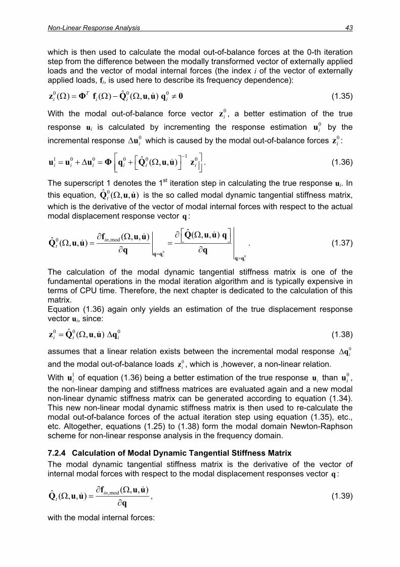
Non-Linear Response Analysis 43
which is then used to calculate the modal out-of-balance forces at the 0-th iteration step from the difference between the modally transformed vector of externally applied loads and the vector of modal internal forces (the index i of the vector of externally applied loads, fi, is used here to describe its frequency dependence):
0 0ˆ( ) ( ) ( , , )Ti i iΩ = Ω − Ω ≠z Φ f Q u u q0
i 0
(1.35)
With the modal out-of-balance force vector z , a better estimation of the true
response u
0i
i is calculated by incrementing the response estimation u by the
incremental response which is caused by the modal out-of-balance forces :
0i
0i∆u 0
iz
11 0 0 0 0 0ˆ ( , , )i i i i t i
− = + ∆ = + Ω u u u Φ q Q u u z . (1.36)
The superscript 1 denotes the 1st iteration step in calculating the true response ui. In this equation, Q is the so called modal dynamic tangential stiffness matrix, which is the derivative of the vector of modal internal forces with respect to the actual modal displacement response vector :
0ˆ ( , , )t Ω u u
q
00
,mod0ˆ ( , , )( , , )ˆ ( , , )
ii
int
==
∂ Ω∂ Ω Ω = =∂ ∂q q
q q
Q u u qf u uQ u u
q q
0i
. (1.37)
The calculation of the modal dynamic tangential stiffness matrix is one of the fundamental operations in the modal iteration algorithm and is typically expensive in terms of CPU time. Therefore, the next chapter is dedicated to the calculation of this matrix. Equation (1.36) again only yields an estimation of the true displacement response vector ui, since:
0 0ˆ ( , , )i t= Ω ∆z Q u u q (1.38)
assumes that a linear relation exists between the incremental modal response 0i∆q
and the modal out-of-balance loads , which is ,however, a non-linear relation. 0iz
With of equation (1.36) being a better estimation of the true response than u , the non-linear damping and stiffness matrices are evaluated again and a new modal non-linear dynamic stiffness matrix can be generated according to equation (1.34). This new non-linear modal dynamic stiffness matrix is then used to re-calculate the modal out-of-balance forces of the actual iteration step using equation (1.35), etc., etc. Altogether, equations (1.25) to (1.38) form the modal domain Newton-Raphson scheme for non-linear response analysis in the frequency domain.
1iu iu 0
i
7.2.4 Calculation of Modal Dynamic Tangential Stiffness Matrix The modal dynamic tangential stiffness matrix is the derivative of the vector of internal modal forces with respect to the modal displacement responses vector q :
,mod ( , , )ˆ ( , , ) int
∂ ΩΩ =
∂f u
Q u uq
u, (1.39)
with the modal internal forces:
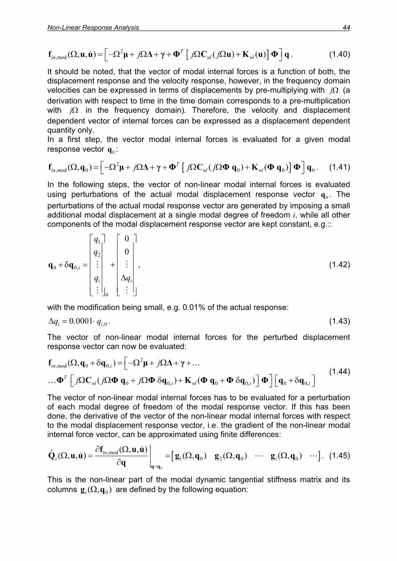
Non-Linear Response Analysis 44
[ ]2,mod ( , , ) ( ) ( )T
in nl nlj j j Ω = −Ω + Ω + + Ω Ω + f u u µ ∆ γ Φ C u K u Φ q . (1.40)
It should be noted, that the vector of modal internal forces is a function of both, the displacement response and the velocity response, however, in the frequency domain velocities can be expressed in terms of displacements by pre-multiplying with jΩ (a derivation with respect to time in the time domain corresponds to a pre-multiplication with jΩ in the frequency domain). Therefore, the velocity and displacement dependent vector of internal forces can be expressed as a displacement dependent quantity only. In a first step, the vector modal internal forces is evaluated for a given modal response vector : 0q
[ ]2,mod 0 0 0 0( , ) ( ) ( )T
in nl nlj j j Ω = −Ω + Ω + + Ω Ω + f q µ ∆ γ Φ C Φ q K Φ q Φ q . (1.41)
In the following steps, the vector of non-linear modal internal forces is evaluated using perturbations of the actual modal displacement response vector q . The perturbations of the actual modal response vector are generated by imposing a small additional modal displacement at a single modal degree of freedom i, while all other components of the modal displacement response vector are kept constant, e.g.::
0
1
2
0 0,
0
00
i
i i
q q
+ δ = + ∆
q q
iq
0,
, (1.42)
with the modification being small, e.g. 0.01% of the actual response:
,00.0001iq∆ = ⋅ . (1.43)
The vector of non-linear modal internal forces for the perturbed displacement response vector can now be evaluated:
2,mod 0 0,
0 0, 0 0, 0
( , )
( ) ( )
in i
Tnl i nl i i
j
j j j
Ω + δ = −Ω + Ω + + Ω Ω + Ω δ + + δ + δ
f q q µ ∆ γ
Φ C Φ q Φ q K Φ q Φ q Φ q q
…
… (1.44)
The vector of non-linear modal internal forces has to be evaluated for a perturbation of each modal degree of freedom of the modal response vector. If this has been done, the derivative of the vector of the non-linear modal internal forces with respect to the modal displacement response vector, i.e. the gradient of the non-linear modal internal force vector, can be approximated using finite differences:
[ ]0
,mod1 0 2 0 0
( , , )ˆ ( , , ) ( , ) ( , ) ( , )int i
=
∂ ΩΩ = = Ω Ω Ω
∂ q q
f u uQ u u g q g q g q
q. (1.45)
This is the non-linear part of the modal dynamic tangential stiffness matrix and its columns are defined by the following equation: 0( , )i Ωg q

Non-Linear Response Analysis 45
,mod 0 0, ,mod 00
( , ) ( , )( , ) in i in
iiq
Ω + δ − ΩΩ =
∆f q q f
g qq
. (1.46)
In contrast to the tangential stiffness matrix of the direct physical response algorithm, each column of the modal tangential stiffness matrix must be calculated, since each modal displacement causes a displacement at each physical degree of freedom. However, since the number of modal degrees of freedom is typically much less than the number of physical degrees of freedom, the calculation of the modal tangential stiffness matrix can be performed quite efficient.
7.3 Concluding Remarks concerning the Iterative Response Calculation
Both, the direct and the modal non-linear frequency response algorithm which were presented above, are similar to the non-linear response algorithms used for non-linear time domain analyses. Whereas in the non-linear time domain algorithms the initial response estimation is coming from the application of a numerical integration scheme (Newmark or Wilson-θ in case of implicit schemes, Central Difference Method in case of explicit schemes), the initial response estimation of the HBResp non-linear frequency response algorithms is coming from the response curve extrapolation. The direct and the modal approach both have advantages and drawbacks, which make one algorithm more suitable for the solution of a specific problem than the other one. In principle, in the modal frequency response algorithm errors are introduced due to modal truncation. This source of inaccuracy is a well known limitation of this approach even for linear response analysis. Furthermore, in non-linear analyses the normal modes of the underlying linear system are used for modal transformation. However, due to the presence of structural non-linearities, the normal modes will change with increasing amplitude of vibration. This means, that the normal modes of the underlying linear system do not decouple the modal domain equations of motion. As a consequence, higher modes with eigenfrequencies far away from the frequency band under consideration during non-linear frequency response analysis may couple with the few modes considered for modal frequency response analysis. The contribution of these high frequency modes to the overall modal frequency response cannot be assessed easily. Nevertheless, it could be proved in the examples in chapter 5, that the modal approach is generally very efficient while maintaining acceptable accuracy. The direct frequency response approach does not include errors related to modal truncation. However, the iterative calculation of the frequency response in physical co-ordinates involves the evaluation and inversion of a large order dynamic tangential stiffness matrix. Furthermore, convergence problems may be encountered if the order of the system matrices is too large. In order to increase the numerical efficiency of this approach, reduction techniques may be applied to the system under consideration to reduce the order of the system matrices prior to response analysis. Another drawback of the direct frequency response approach is the generation of the physical damping matrix. This matrix is calculated from a superposition of the contributions of linear and non-linear elements, where the non-linear contribution is generally response dependent. However, the linear part of the physical damping matrix is typically unknown, because physical dampers are rarely defined in a finite element model.
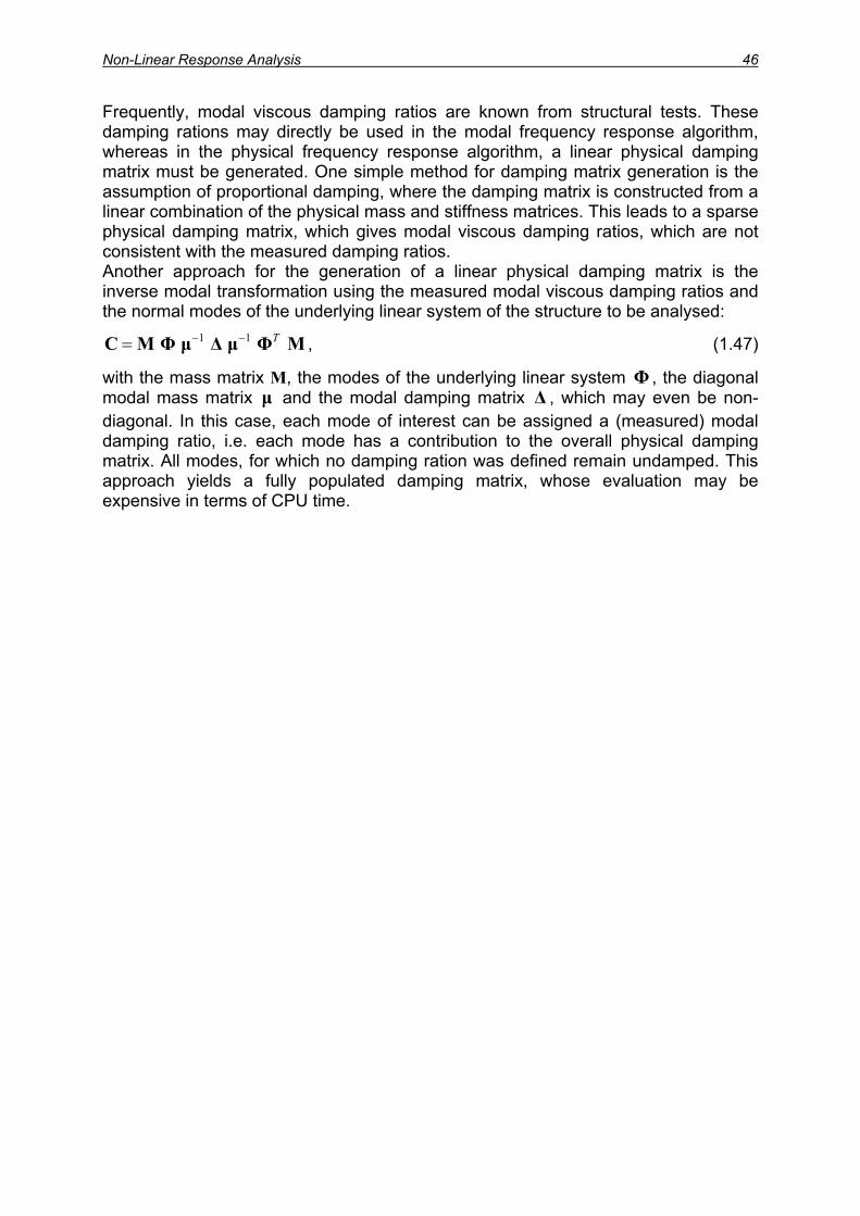
Non-Linear Response Analysis 46
Frequently, modal viscous damping ratios are known from structural tests. These damping rations may directly be used in the modal frequency response algorithm, whereas in the physical frequency response algorithm, a linear physical damping matrix must be generated. One simple method for damping matrix generation is the assumption of proportional damping, where the damping matrix is constructed from a linear combination of the physical mass and stiffness matrices. This leads to a sparse physical damping matrix, which gives modal viscous damping ratios, which are not consistent with the measured damping ratios. Another approach for the generation of a linear physical damping matrix is the inverse modal transformation using the measured modal viscous damping ratios and the normal modes of the underlying linear system of the structure to be analysed:
1 1 T− −=C M Φ µ ∆ µ Φ M , (1.47)
with the mass matrix M, the modes of the underlying linear system , the diagonal modal mass matrix µ and the modal damping matrix , which may even be non-diagonal. In this case, each mode of interest can be assigned a (measured) modal damping ratio, i.e. each mode has a contribution to the overall physical damping matrix. All modes, for which no damping ration was defined remain undamped. This approach yields a fully populated damping matrix, whose evaluation may be expensive in terms of CPU time.
Φ∆

Non-Linear Response Analysis 47
8 Control Facilities of the Iteration Algorithm It is a basic requirement for an iteration algorithm to be effective and to avoid unnecessary iterations wherever possible. This involves the termination of the iteration, when either the last calculated response fulfils a certain convergence criterion, or if divergence is detected if a certain divergence criterion is fulfilled. Both, convergence and divergence criteria, together with the tangential stiffness matrix update strategy involved in the iteration are discussed in this chapter. Note: The convergence and divergence criteria and their tolerances presented in the remainder of this chapter are based on the MSC.Nastran™ non-linear time domain iteration algorithm. Although this algorithm operates in the time domain, the definition of the convergence and divergence criteria as well as the tolerances were found to be applicable to non-linear frequency domain analysis. This was proved by a number of non-linear frequency response analyses using these criteria and tolerances adopted from MSC.Nastran™.
8.1 Convergence Conditions An iterative calculation continues until convergence is obtained by satisfying a certain convergence criteria. The residual error vector (out-of-balance forces) at a certain iteration step is used to calculate a change in displacements, which are then carried over to the next iteration step. When convergence criteria are satisfied, the out-of-balance forces and the changes in displacements should be sufficiently small such that the remaining error is no longer physically significant nor will it cause any adverse effects, numerically or physically, on the succeeding incremental steps. Convergence tolerances have the following effects on the performance of an iteration algorithm (in terms of CPU time and in terms of accuracy):
• excessively tight tolerances will cause a waste of computing resources for unnecessary iterations to achieve accuracy;
• excessively loose tolerances will cause not only inaccuracy but also convergence difficulties in the subsequent steps due to cumulative errors.
The most natural and reasonable criterion for the convergence test is formulated in terms of energy error. The energy error is a logical choice because both, the out-of-balance forces r and the change in displacements ∆u should be minimised by the iteration process. Although the convergence test in terms of energy errors is usually adequate, some errors are not detected with this criterion; e.g. when displacements are in gross error while the residual load error is negligible, or vice versa. Thus, a second convergence test is formulated in terms of error force, which must be fulfilled at the same time in case of a converged solution. A third independent convergence test might be defined in terms of displacement errors. This displacement based convergence criterion is mainly based on negligible changes in displacements if convergence is approached. Nominally, by visualising the load-deflection curve for a one-dimensional non-linear system, it can be observed that the criterion in terms of load governs stiffening structures, whereas the criterion in terms of displacements governs softening structures. However, the convergence criterion in terms of error energy combines both, errors in force and errors in displacement. All the error functions are defined as relative errors in terms of vector norms. The vector norm is defined by a sum of the absolute values of the vector components. The vectors used in these norms, however, are not raw vectors but are weighted vectors using other vector quantities as weighting factors. The weighting factors are

Non-Linear Response Analysis 48
chosen in such a way, that the products have common and consistent structural units. In all cases, the convergence criteria should meet the following requirements:
• be satisfied for linear cases at all times • be independent of structural units • be reliable • render consistent accuracy • be independent of structural characteristics (stiffening or softening)
The HBResp non-linear frequency response algorithms use both, the convergence criterion in terms of error energy and the convergence criterion in terms of error force, to detect convergence of the iteration. Both criteria are discussed below.
8.1.1 Convergence Criterion in terms of Error Energy The relative error in terms of energy is defined by equation (2.1). The energy error is normalised by another energy quantity that is relatively stable throughout the analysis:
*wEE∗∆
=r u
, (2.1)
with:
( )2j j
jr u∗∆ = ∆∑r u , (2.2)
and:
( )2*j j
jE = ∗ = ∑f u f u , (2.3)
where r represents the out-of-balance forces at the current iteration, represents the incremental displacement at the current iteration, f is the vector of externally applied loads, and u represents the total displacements at the current iteration.
∆u
8.1.2 Convergence Criterion in terms of Error Force The error function in terms of force is made dimensionless by a weighted normalisation using the total displacement vector:
fE∗
=∗
r uf u
, (2.4)
in which the numerator is:
( )2j j
jr u∗ = ∑r u , (2.5)
and the denominator is the same as for the error energy and is defined in equation (2.3).

Non-Linear Response Analysis 49
8.1.3 Convergence Tolerances The convergence tolerance determines the efficiency of the solution scheme as well as the accuracy of the solution. The tolerance should be realistic, not too tight nor too loose. It is difficult to choose optimal default values for the convergence tolerances. However, one could make a benefit form the default values defined for standard finite element software, e.g. for the MSC.Nastran™ non-linear time domain algorithms. It was mentioned before, that the HBResp convergence criteria were adopted from MSC.Nastran™ non-linear time domain algorithm. Efforts have been made by the MSC.Nastran™ developers to set the default values of the convergence tolerances to provide reliable solutions to a general class of problems. Thus, those default tolerances specified for MSC.Nastran™ non-linear time domain algorithm should be adhered to until good reasons are found to change them. The convergence test is performed in each iteration, after the displacement response was incremented by the displacement response caused by the out-of-balance forces. The convergence tolerances for the error functions in terms of error energy Ew and in terms of error force Ef are defined as follows (note that these values have no physical unit):
710w wE −≤ ε = , (2.6)
310f fE −≤ ε = . (2.7)
These values are a result of a study using 47 different non-linear problems which were analysed using the MSC.Nastran™ non-linear time domain algorithm. Changes to these default values can be made in the HBResp settings file 'hbset.m'.
8.2 Divergence Criterion and Tangent Stiffness Matrix Update Strategy
An iteration algorithm is considered efficient if unnecessary iterations are avoided whenever possible. This involves the detection of a diverging solution in an early stage of the iterative calculation. There are two classifications for divergence conditions: probable and absolute divergence, where the absolute divergence is treated as two occurrences of the probable divergence. Divergence criteria are defined based on the ratio of energy errors evaluated before and after iteration, i.e. for the i-th iteration:
1
Ti i idiv T
i i
E−
∆ ⋅=∆ ⋅
u ru r
, (2.8)
with being the incremental displacement response caused by the out-of-balance forces r. Then, the divergence criteria are established as follows:
∆u
• Absolute divergence if: 51 10i
divE −> + or , (2.9) 1210idivE < −
• Probable divergence if: 1210 1i
divE− < < − . (2.10) Again, the default values for the detection of a diverging solution were adopted from MSC.Nastran™ non-linear time domain algorithm. If a diverging solution is detected a new tangential stiffness matrix will be calculated, i.e. this matrix will be updated. The tangential stiffness matrix update is controlled by

Non-Linear Response Analysis 50
an internal HBResp variable Ndiv, which is initially set to zero at the beginning of the iteration, e.g. when the solution at a certain frequency point has converged and the solution at the succeeding frequency point has to be calculated. If an absolute divergence condition is detected from evaluating the divergence criterion, equation (2.8), the internal variable Ndiv is incremented by 2; if a probable divergence condition is detected, the internal variable Ndiv is incremented by 1. The solution is considered to diverge, if the internal variable Ndiv exceeds a user defined value maxdiv:
maxdiv divN ≥ . (2.11)
The default value for Ndiv is 2, e.g. two probable divergence conditions are allowed to be detected or, respectively, one absolute divergence condition, before the solution is considered diverging. Changes to the default values can be made in the HBResp settings file 'hbset.m'. It was mentioned before that the calculation of the tangential stiffness matrix is the most expensive step in terms of CPU time of an iterative non-linear frequency response calculation. In order to make the iteration algorithm efficient, the calculation of the tangential stiffness matrix is not performed in each iteration step. In case of a divergent solution or in case that kstep iterations have been performed without a new evaluation of the tangential stiffness matrix, it will be updated automatically. This is equivalent to the 'Modified Newton-Raphson' scheme and its application can be justified by the fact, that the non-linear frequency response curve typically has regions, where the response is very small and smooth (negligible non-linear effects), and regions, where the non-linearities cause significant distortions from the linear response. In the smooth regions, which are typically located far away from the resonance peaks, the changes in the tangent stiffness matrix are negligible and the response calculation can be performed efficiently without the need to update the tangential stiffness matrix in each iteration step.

Non-Linear Response Analysis 51
8.3 Flow Chart of the Direct Physical Non-Linear Iteration Algorithm
Figure 19: Flow chart of direct physical non-linear iteration algorithm

Non-Linear Response Analysis 52
8.4 Flow Chart of the Modal Non-Linear Iteration Algorithm
Figure 20: Flow chart of the modal non-linear iteration algorithm

Example Problem 53
9 HBResp DMAPs for MSC.Nastran™ Two DMAPs (Direct Matrix Abstraction Programming) are delivered with HBResp software. These DMAPs must be included in the MSC.Nastran™ input files to enforce that certain data blocks and system matrices are exported form MSC.Nastran™ into binary files.
9.1 DMAP MEXPORT.V707 This DMAP enforces the export of the system matrices of the MSC.Nastran™ a-set degrees of freedom. At this stage of the solution sequence, all multi point constraints, single point constraints, Craig-Bampton reductions, and Guyan reductions have been performed. Since a standard DMAP label is used to include the DMAP alters in the solution sequence 103, this DMAP is independent of the MSC.Nastran™ version and should work for future versions of MSC.Nastran™ as well. Below is a listing of the DMAP: $ ECHOOFF $ ------------------------------------------------------------------------------ $ This is a DMAP for the export of the residual structure's system matrices of a $ Nastran Superelement model. The system matrices are exported to a binary *.op4 $ file (Unit 31). $ $ This DMAP was designed and tested under Nastran Versions 70.5, 70.7 and 2001. $ However, since this DMAP uses a standard label in conjunction with the MALTER $ statement this DMAP should also work for future Nastran Versions. $ $ Author: University of Kassel $ Civil Engineering Department $ Lightweight Structures and Structural Mechanics Laboratory $ Dipl.-Ing. Marc Boeswald $ $ Date : 15.10.2003 $ $ Note: In order to write the desired information to the corresponding files the $ following statements must be included at the to of in the Input File: $ ASSIGN OUTPUT4 = 'Filename.op4', UNIT = 31 $ $ Furthermore, this DMAP must be included into the Nastran Input File by $ using an include statement (before CEND statement), e.g. : $ INCLUDE 'C:\User\DMAP\MEXPORT.V707' $ ------------------------------------------------------------------------------ $ MALTER 'MALTER:AFTER SUPERELEMENT MATRIX AND LOAD REDUCTION TO A-SET' $ IF (SEID = 0) THEN $ $ Write Matrices KAA and MAA in Binary Format to the File generated by Unit 31 MESSAGE //' ### Write Matrices Kaa and Maa to OP4 File for SE '/SEID $ OUTPUT4 KAA,MAA//-1/-31/1/TRUE/9 $ $ Export USET Table to standard OP2 File generated by Unit 12 MESSAGE //' ### Write USET Table to OP2 File '/$ OUTPUT2 USET//0/12///'USET' $ $ $ End Analysis after Exporting the Matrices (if requested) $ Note: No modal data will be available if the run is terminated here! $ EXIT $ ENDIF $ ENDALTER $ ECHOON $
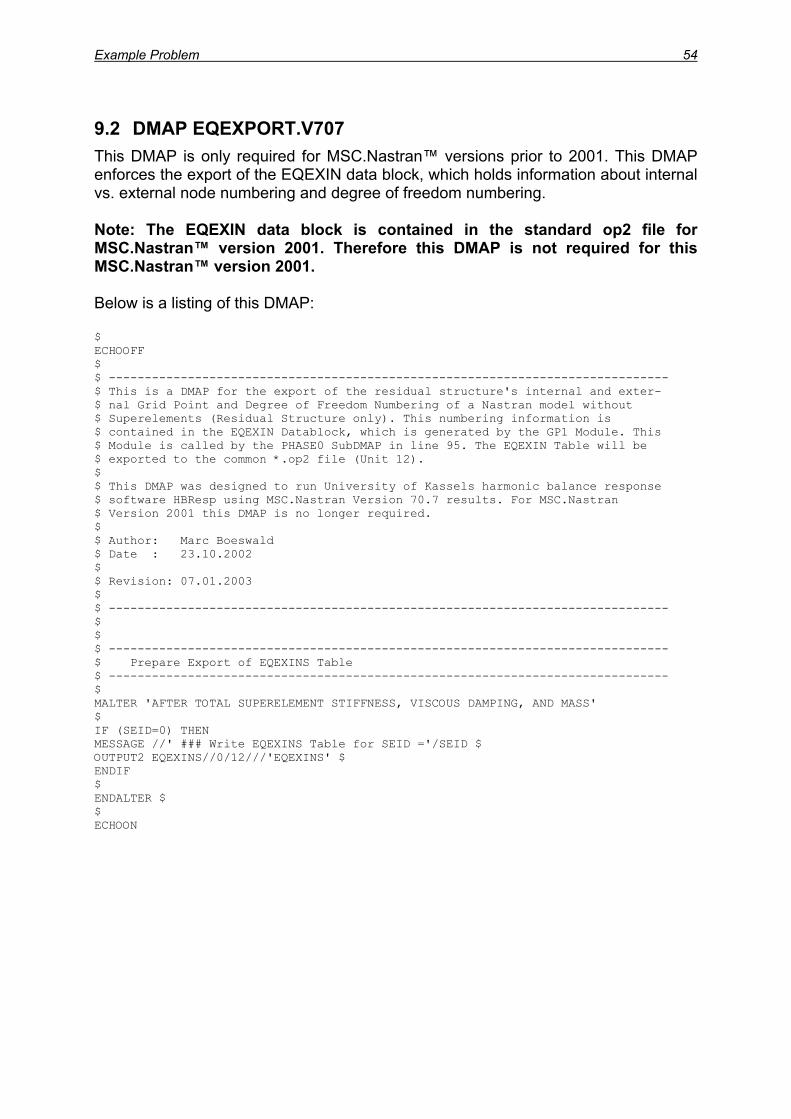
Example Problem 54
9.2 DMAP EQEXPORT.V707 This DMAP is only required for MSC.Nastran™ versions prior to 2001. This DMAP enforces the export of the EQEXIN data block, which holds information about internal vs. external node numbering and degree of freedom numbering. Note: The EQEXIN data block is contained in the standard op2 file for MSC.Nastran™ version 2001. Therefore this DMAP is not required for this MSC.Nastran™ version 2001. Below is a listing of this DMAP: $ ECHOOFF $ $ ------------------------------------------------------------------------------ $ This is a DMAP for the export of the residual structure's internal and exter- $ nal Grid Point and Degree of Freedom Numbering of a Nastran model without $ Superelements (Residual Structure only). This numbering information is $ contained in the EQEXIN Datablock, which is generated by the GP1 Module. This $ Module is called by the PHASE0 SubDMAP in line 95. The EQEXIN Table will be $ exported to the common *.op2 file (Unit 12). $ $ This DMAP was designed to run University of Kassels harmonic balance response $ software HBResp using MSC.Nastran Version 70.7 results. For MSC.Nastran $ Version 2001 this DMAP is no longer required. $ $ Author: Marc Boeswald $ Date : 23.10.2002 $ $ Revision: 07.01.2003 $ $ ------------------------------------------------------------------------------ $ $ $ ------------------------------------------------------------------------------ $ Prepare Export of EQEXINS Table $ ------------------------------------------------------------------------------ $ MALTER 'AFTER TOTAL SUPERELEMENT STIFFNESS, VISCOUS DAMPING, AND MASS' $ IF (SEID=0) THEN MESSAGE //' ### Write EQEXINS Table for SEID ='/SEID $ OUTPUT2 EQEXINS//0/12///'EQEXINS' $ ENDIF $ ENDALTER $ $ ECHOON

Example Problem 55
10 Example Problem: Beam Model with Non-Linear Joint In this chapter, the HBResp user is guided through an example problem in order to become familiar with the software and its graphical user interface (GUI). The example considered consists of a cantilever beam, which is assembled of two components with a tuning mass at the free beam end ( ). This example has been used in the development of the non-linear iteration algorithm as well as in [Boeswald 02b].
Figure 21
Figure 21: Beam Model of Cylindrical Test Structure (CTS)
Figure 21
tuning mass
component 2
component 1
stiffness of support
joint model
Below, the MSC.Nastran™ input deck for the underlying linear system of this example problem is listed. The joint between the two beam components is represented by a linear rotational spring and a non-linear rotational element having a cubic softening character and a quadratic damping character2. The linear part is modelled within MSC.Nastran™, whereas the non-linear part is modelled within HBResp. The inclusion of the HBResp DMAPs will enforce the export of the system matrices, the USET data block, and the EQEXIN data block. $ ------------------------------------------------------------------------------ $ $ This is a Nastran Input Deck of the underlying linear System of the CTS Beam $ Model which is used as an Example Problem in the HBResp Harmonic Balance $ Response Analysis Software developed by University of Kassel. $ $ Date: 17.12.2002 $ Author: Marc Böswald $ $ ------------------------------------------------------------------------------ $ ASSIGN OUTPUT2 = 'CTS_Beam.op2', UNIT = 12 $ $ Assign OP4-File for system matrices (created by Fortran Unit 31) ------------- ASSIGN OUTPUT4 = 'CTS_Beam.op4', UNIT = 31 $ ------------------------------------------------------------------------------ $ SOL 103 $ $ Include HBResp DMAP to export system matrices to OP4 File -------------------- INCLUDE 'c:\ukl\hbresp\DMAP\MEXPORT.V707' $ INCLUDE 'c:\ukl\hbresp\DMAP\EQEXPORT.V707' $ ------------------------------------------------------------------------------ $ CEND
2 The joint of the structure shown in is modelled using rotational although it is pictured with translational springs.

Example Problem 56
TITLE = Beam Model of Cylindrical Test Structure CTS ECHO = NONE SUBCASE 1 METHOD = 1 SPC = 2 VECTOR(SORT1,REAL)=ALL $ $ BEGIN BULK $ $ $ Analysis Parameters ---------------------------------------------------------- PARAM,POST,-1 PARAM,COUPMASS,1 PARAM,GRDPNT,0 PARAM,NOCOMPS,-1 PARAM,PRTMAXIM,YES EIGRL 1 6 0 MASS $ ------------------------------------------------------------------------------ $ $ $ Nodes of the Entire Model ---------------------------------------------------- GRID 1 0. 0. 0. GRID 2 0. 0. 62.125 GRID 3 0. 0. 124.25 GRID 4 0. 0. 186.375 GRID 5 0. 0. 248.5 GRID 6 0. 0. 248.5 GRID 7 0. 0. 310.625 GRID 8 0. 0. 372.75 GRID 9 0. 0. 434.875 GRID 10 0. 0. 497. GRID 11 0. 0. 512. $ ------------------------------------------------------------------------------ $ $ $ Material Record : Steel ------------------------------------------------------ MAT1 1 204750. .3 8.05-9 $ ------------------------------------------------------------------------------ $ $ $ Beam Elements representing the cylindrical Components ------------------------ PBAR 2 1 1577.07 1.242+7 1.242+7 2.484+7 + .5 .5 0. CBAR 1 2 1 2 1. 0. 0. CBAR 2 2 2 3 1. 0. 0. CBAR 3 2 3 4 1. 0. 0. CBAR 4 2 4 5 1. 0. 0. CBAR 5 2 6 7 1. 0. 0. CBAR 6 2 7 8 1. 0. 0. CBAR 7 2 8 9 1. 0. 0. CBAR 8 2 9 10 1. 0. 0. $ ------------------------------------------------------------------------------ $ $ $ Rotational Spring at fixed Beam End to simualte Support Stiffness ------------ PELAS* 1 1.+10 * CELAS1 11 1 1 5 $ ------------------------------------------------------------------------------ $ $ $ Rotational Spring to join the rotational DOFs of the Beam Segments ----------- PELAS 3 2.825+9 CELAS1 10 3 5 5 6 5 $ ------------------------------------------------------------------------------ $ $ $ Tuning Mass at the free Beam End ---------------------------------------------

Example Problem 57
CONM2 9 10 0 .02295 357.171 357.171 355.450 $ ------------------------------------------------------------------------------ $ $ Masses of the different Flanges ---------------------------------------------- CONM2 14 10 0 4.55E-4 CONM2 15 5 0 7.7E-5 CONM2 16 6 0 7.7E-5 $ ------------------------------------------------------------------------------ $ $ Rigid Body Elements ---------------------------------------------------------- $ Join Tuning Mass and free Beam End rigidly RBAR 12 10 11 123456 15 $ Join Beam Components rigidly for translational DOFs RBAR 13 6 5 123456 1 $ ------------------------------------------------------------------------------ $ $ $ Boundary Conditions ---------------------------------------------------------- SPCADD 2 1 3 $ Planar Beam Problem: Constrain all DOF which would cause out of plane motion SPC1 1 2346 1 THRU 11 $ Constrain translational DOF at fixed End SPC1 3 1 1 $ ------------------------------------------------------------------------------ $ $ ENDDATA
Six eigenfrequencies are calculated for the underlying linear system of the beam structure shown in Figure 21:
Table 1: Eigenfrequencies of CTS Beam Model
Number Frequency [Hz]1 114,192 649,233 1930,834 4275,035 6171,046 9136,91
If the MSC.Nastran™ model with the HBResp DMAPs has been analysed, a linear and non-linear frequency response analysis up to 1000 Hz shall be performed using HBResp. In this case, only the first two modes need to be considered. To start HBResp, first start MATLAB™ and then move to the directory, where the HBResp result files shall be generated (use the ‘cdir’ command to change the directory). Note: This directory does not have to be the directory which contains the MSC.Nastran™ results: >> cdir HBResp is started by entering 'hbresp' at the MATLAB™ prompt: >> hbresp

Example Problem 58
The ‘HBResp Main Window’ will appear (Figure 22).
enter jobname
enter title
Figure 22: HBResp Main Window
Figure 22In order to import the MSC.Nastran™ model data, a jobname must be entered and an optional analysis title can be entered ( ). Then the MSC.Nastran™ model data is imported by activating the 'Import Nastran Model' pushbutton. The following output appears on the MATLAB™ command window » Reading GEOM1S table (GRID data). Reading GEOM4S table (RBAR). Reading GEOM4S table (SPC1). Reading EQEXINS table (internal vs. external numbering). Reading OUGV1 table (real mode 1). Reading OUGV1 table (real mode 2). Reading OUGV1 table (real mode 3). Reading OUGV1 table (real mode 4). Reading OUGV1 table (real mode 5). Reading OUGV1 table (real mode 6). The HBResp database files jobname.mtx, jobname.nas, jobname.pld will be created in the current working directory. These files can directly be used for future analyses by using the 'Search' pushbutton (Figure 22), e.g. the MSC.Nastran™ model data has only to be imported once. The parameters for the frequency response analysis must be defined. This can be done via the ‘Analysis Parameter Window’, which appears after the pushbutton 'Define Parameters' has been activated.

Example Problem 59
select modes
select exciter DOFs
select response DOFs
enter damping values
select type of damping
define frequency range
enter force amplitudes select analysis
approach
select output settings
Figure 23: Analysis Parameter Window
Figure 23Select the first two modes for the frequency response analysis in the upper left hand side frame of the ‘Analysis Parameter Window’ ( ). (Multiple modes can be selected from the listbox by mouse picking in conjunction with the CTRL key.) After the modes have been selected, the type of damping must be defined. Different approaches for damping are available. The most convenient one is 'diagonal modal Damping Matrix', where the user can enter viscous modal damping ratios in percent of critical damping. In this example, the two selected modes may both have a viscous modal damping ratio of 0.54%. To define this type of damping, first select the type of damping 'diagonal modal Damping Matrix' from the popup menu in the upper right hand side frame of the ‘Analysis Parameter Window’, Figure 23. Then enter the damping ratios into the edit field below the popup menu in the upper right frame: [0.54 0.54] After damping has been defined, the excitation force and position must be defined. This is done in the left hand side frame in the middle of the ‘Analysis Parameter Window’. First select all exciter DOFs and then enter the corresponding excitation force amplitudes in the edit field below the listbox. For this example, select node 11, direction T1 as the exciter degree of freedom. Assign a 10N excitation force amplitude to this exciter DOF:

Example Problem 60
[10] The selection of the response degrees of freedom is done in the right hand side frame of the ‘Analysis Parameter Window’. Generally, the selection of response degrees of freedom is done in the same way as the selection of exciter degrees of freedom. For this example, select node 11, direction T1 as a response degree of freedom. In the next step, the frequency range for the frequency response analysis must be defined (lower left hand side frame of the ‘Analysis Parameter Window’). For this example, enter the lower frequency limit: 0 the upper frequency limit 1000 and the number of frequency points: 1001 For non-linear frequency response analysis, the step direction may be important. The user can select 'Run-Up', 'Run-Down', or 'Run-Up and Run-Down'. For this example select 'Run-Up and Run-Down' to request the frequency response for both. In the lower right hand side frame of the ‘Analysis Parameter Window’, the analysis approach can be selected. The 'modal' and the 'direct' frequency response are available. Even if a direct frequency response is selected you can use the viscous modal damping ratios to generate the physical damping matrix. For this example select the 'modal' response approach and activate the checkbox for 'Plot Response after Analysis' while deactivate the checkbox for 'Calculate and Plot Mode Indicator Function'. In addition, select all available options from the listbox 'Analysis Status Display Options' to request a maximum of output in the HBResp log file jobname.aus. If now the pushbutton 'Create Input File' is activated, the HBResp database files jobname.ctr and jobname.frc are created in the current directory. Once these files are created, they can be loaded by using the 'Load Input File' pushbutton. The parameters defined in these files are re-constructed on the ‘Analysis Parameter Window’ and can be altered to create new jobname.ctr and jobname.frc database files. If the 'Cancel' pushbutton is activated, the ‘Analysis Parameter Window’ is closed without saving the settings which may have been made.

Example Problem 61
If the frequency response analysis parameters have been defined, the linear frequency response can be calculated by activating the 'Run Linear Analysis' pushbutton on the ‘HBResp Main Window’. The linear response is calculated and plotted:
Figure 24: HBResp Linear Response Window
The upper left hand side frame shows the imaginary part of the acceleration frequency response, whereas the lower left hand side frame shows the real part of the acceleration frequency response. The upper right hand side frame shows the mode indicator function due to the selected excitation. The results of the linear response analysis are stored in the files jobname.rp1, jobname.rp2 and jobname.rp3. The linear frequency response data can be loaded by using the MATLAB™ command: load jobname.rp2 –mat load jobname.rp3 –mat subplot(2,1,1),plot(fe,Uim) subplot(2,1,2),plot(fe,Ure) See MATLAB™ 'plot' command for details of plotting response curves. After the linear response was calculated, the non-linear elements can be introduced. This is done by activating the 'Define Non-Linearity' pushbutton on the ‘HBResp Main Window’ (Figure 22). The user is asked to select a MATLAB™ m-file containing the celas and pelas matrices which define the geometry and the properties of the non-linear elements.

Example Problem 62
For the CTS beam model, this m-file has the following content: % EID PID GA GB C celas = [ 1 1 5 6 5 ]; % PID TYPE Knl pk Cnl pc pelas = [ 1 111 -1.4e15 3 3.75e5 2 ]; A non-linear (relative) spring-damper element will be added to the system matrices between degree of freedom components 5 of the nodes 5 and 6 (rotation about the y-axis). After the non-linear elements have been defined a non-linear frequency response analysis can be performed by activating the 'Run Non-Linear Analysis' pushbutton. The non-linear response plots are shown below. On the left hand side of the real/imaginary part of the non-linear frequency response is shown, whereas on the right hand side the magnitude/phase of the non-linear frequency response is plotted
Figure 25
Figure 25: Non-linear Frequency Response Plots
The results of the non-linear frequency response plots are stored in the following files: jobname.rp4: real part of acceleration response for 'Run-Up' jobname.rp5: imaginary part of acceleration response for 'Run-Up' jobname.rp6: real part of acceleration response for 'Run-Down' jobname.rp7: imaginary part of acceleration response for 'Run-Down' The non-linear frequency response data can be loaded by using the MATLAB™ command: load jobname.rp4 –mat load jobname.rp5 –mat load jobname.rp6 –mat load jobname.rp7 –mat subplot(2,1,1),plot(fe,Aim_nl_u,fe,Aim_nl_d) subplot(2,1,2),plot(fe,Are_nl_u,fe,Are_nl_d)

Example Problem 63
See MATLAB™ 'plot' command for details of plotting response curves. After the complete response between 0 Hz and 1000 Hz was calculated, the response in the vicinity of the first mode shall be analysed in detail. Therefore, close the response windows and return to the ‘HBResp Main Window’. Activate the 'Define Parameters' pushbutton to define the frequency response analysis parameters for the new the frequency response analysis. The HBResp ‘Analysis Parameter Window’ appears. Activate the 'Load Input File' pushbutton on the ‘Analysis Parameter Window’ and select the jobname.ctr file to load the previously defined parameters. Now the frequency range can be altered. Enter the new lower frequency limit: 105 the new upper frequency limit 125 and the new number of frequency points: 201 Change the step direction to 'Run-Up and Run-Down' (should already be set). Furthermore, change the excitation force amplitude from 10 N to 80 N. After activating the 'Create Input File' pushbutton the new analysis parameters are stored in the jobname.ctr and jobname.frc database files (the old files will be overwritten). A new linear response analysis must be performed after the analysis parameters have been changed. This is done by activating the 'Run Linear Analysis' pushbutton. The linear response in the vicinity of mode 1 is shown in Figure 26
Figure 26: Linear Response in the Vicinity of Mode 1
Again, the non-linear elements must be defined by activating the 'Define Non-Linearity' pushbutton. Then the non-linear response analysis can be started by activating the 'Run Non-Linear Analysis' pushbutton.

Example Problem 64
Figure 27: Non-linear Response Plots for 80N Excitation Force
It can be seen form Figure 27 that the non-linear frequency response curves for 'Run-Up' and 'Run-Down' are identical. This means, that there is no unstable region of the non-linear response curve and therefore no bifurcation of the non-linear response (jump phenomenon) occurs. A jump phenomenon will occur if the load is further increased up to 170 N. This can be observed from (Figure 28), where the response curve for ‘Run-Up’ and ‘Run-Down’ are different.
Figure 28: Non-linear Response Plots for 170 N Excitation Force
Note: Each time a new non-linear analysis is performed, the results files jobname.rp* are renamed with a new file extension. The most recently calculated response is stored in the files without additional file extension.
System of Units 65
11 Known Limitations In this chapter, the known limitations of HBResp are discussed.
11.1 Superelement Analysis MSC.Nastran™ distinguishes between two different superelement analysis approaches, namely, the 'Main Bulk Data Superelements' (cookie-cutter approach) and the 'PARTs Superelements' ("component models" approach), see [Nastran 01]. If Main Bulk Data superelements are defined, the superelement´s interior grid points (slave degrees of freeom) must be assigned by the user via SESET and SESET1 bulk data cards. The superelement´s exterior grid points (master degrees of freedom) are automatically detected and the superelement´s elements, loads, and constraints are automatically partitioned by MSC.Nastran™ based on interior grid point assignments. If PARTs superelements are defined, the bulk data deck of a MSC.Nastran™ input file is subdivided into several sections; one section for each superelement. The BEGIN statement is used as a terminator for each section, whereas the last section is terminated by the ENDATA statement. This means, that all bulk data cards between two BEGIN statements (or respectively between a BEGIN statement and the ENDDATA statement) belong to a certain superelement. MSC.Nastran™ automatically determines the exterior and interior grid points of each superelement from the coincidence information of the boundary nodes of the different superelements. In this case, the coincident boundary nodes of two adjacent superelements will be merged automatically, such that no additional springs may be defined between the two adjacent superelements in order to represent a certain joint stiffness. In HBResp version 1.1 the PARTs superelements were definitely not supported. However, in HBResp version 1.2, a different approach for the reconstruction of the MSC.Nastran™ displacement sets (g-set, m-set, s-set, o-set , q-set, and a-set) is used, i.e. using PARTs superelements should no longer be a restriction for using HBResp. This, however, has not been approved (comments are welcome!). There restrictions of HBResp version 1.1 no longer apply to HBResp version 1.2, since the USET data block is used directly, instead of reconstructing the a-set from the SESET and SEQSET cards.
11.2 Rigid Body Elements In contrast to HBResp version 1.1, HBResp version 1.2 uses the USET data block for the reconstruction of the MSC.Nastran™ displacement sets (incl. the m-set). This means, that the restriction to only use RBAR and RBE2 elements to define constraints between multiple degrees of freedom is no longer active in HBResp version 1.2.

System of Units 66
11.3 Boundary Conditions In contrast to HBResp version 1.1, HBResp version 1.2 uses the USET data block for the reconstruction of the MSC.Nastran™ displacement sets (incl. the s-set). This means, that the restriction to only use SPC and SPC1 cards to model displacement boundary conditions is no longer active in HBResp version 1.2.
11.4 Static Condensation In contrast to HBResp version 1.1, HBResp version 1.2 uses the USET data block for the reconstruction of the MSC.Nastran™ displacement sets (incl. the o-set). This means, that the restriction to only use ASET and ASET1 cards of static condensation is no longer active in HBResp version 1.2.

System of Units 67
12 System of Units Since the database of HBResp is imported from MSC.Nastran™ the system of units used for frequency response analysis is the unit system which was used for model description. Three consistent unit systems applicable for finite element analysis are listed below.
Table 2: Unit Systems for Finite Element Analysis
phys. Quantity [m k s] System [mm t s] System [cm g s] SystemLength meters [m] millimeters [mm] centimeters [cm]Mass kilogramms [kg] tonns [t] gramms [g]Time seconds [s] seconds [s] seconds [s]
Acceleration [m/s2] [mm/s2] [cm/s2]Velocity [m/s] [mm/s] [cm/s]
Displacement [m] [mm] [cm]Force Newtons [N] Newtons [N] [(g cm)/s2]
Pressure [N/m2] [N/mm2] [g/(cm s2)]Density [kg/m3] [t/mm3] [g/cm3]
Youngs Modulus [N/m2] [N/mm2] [g/(cm s2)] The [m k s] system is the so called SI unit system. Note: If the model which was imported from MSC.Nastran™ is defined in the [mm t s] system, then the acceleration frequency response calculated by HBResp is in physical unit [mm/s2]. Since the model can be defined in any unit system, no physical units are displayed in the response plots.

Fixed Variable Names 68
13 Fixed Variable Names In this chapter, the fixed variable names of the different HBResp database files are briefly discussed. Sizes of matrices and vectors are depend on the model size and on the analysis parameters selected.
13.1 Content of HBResp database file jobname.ctr C physical damping matrix DOF_r response degree of freedom DOFa_r response degree of freedom (a-set) addf index of eigenfrequency to be included in frequency range of analysis damptyp type of damping flow lower frequency limit fup upper frequency limit imif index for calculation of multivariate mode indicator function kind_it iteration approach knresp response node numbers name_modalresp jobname nresp number of response degrees of freedom plotresp index for response plot plotresp_par not used prop_d vector of proportional damping factors [alpha beta] riresp direction of response degrees of freedom step_dir step direction (run-up, run-down, or both) stepno number of frequency points in frequency range sw_display vector of analysis status display options xeffno number of modes selected xsi diagonal of viscous modal damping ratios xsid viscous modal damping matrix
13.2 Content of HBResp database file jobname.frc DOF_f exciter degree of freedom number DOFa_f exciter degree of freedom number (a-set) F force amplitudes knr node numbers excitation of excitation nodes nef total number of exciter degrees of freedom ril direction of excitation
13.3 Content of HBResp database file jobname.koi beam_type vector of non-linear element type number kol node numbers of non-linear elements kor unused
13.4 Content of HBResp database file jobname.mod Xges modal matrix of MSC.Nastran model (all dofs) fv vector of natural frequencies of MSC.Nastran model mue vector of modal masses x modal matrix of MSC.Nastran model (a-set dofs)

Fixed Variable Names 69
13.5 Content of HBResp database file jobname.mtx EKaa unused EMaa unused Fei unused Ffpg unused K stiffness matrix of MSC.Nastran model (a-set) Ke unused Kekoin degrees of freedom of non-linear elements in a-set Kes unused Keskoin unused M mass matrix of MSC.Nastran model (a-set) MF_RUNID unused Me unused Mekoin unused Mes unused Meskoin unused Mstarr unused koin unused mkel unused va a-set vector (unit vector of length M(:,1)) vb unused
13.6 Content of HBResp database file jobname.nas aset members of a-set eqexin_aset extended internal vs. external numbering fv vector of natural frequencies grid_points co-ordinates and co-ordinate systems of grid points
13.7 Content of HBResp database file jobname.nlp C_nl_par parameters of non-linear dampers K_nl_par parameters of non-linear springs MF_RUNID unused step_dir step direction (run-up, run-down, both)
13.8 Content of HBResp database file jobname.pld koord grid point co-ordinates ueberschrift analysis title
13.9 Content of HBResp database file jobname.prp MF_RUNID unused elementdat non-linear element data nbalk unused nshel unused nshel3 unused nshel4 unused qxyz_b unused qxyz_s unused struct_par unused teta_b unused teta_s unused
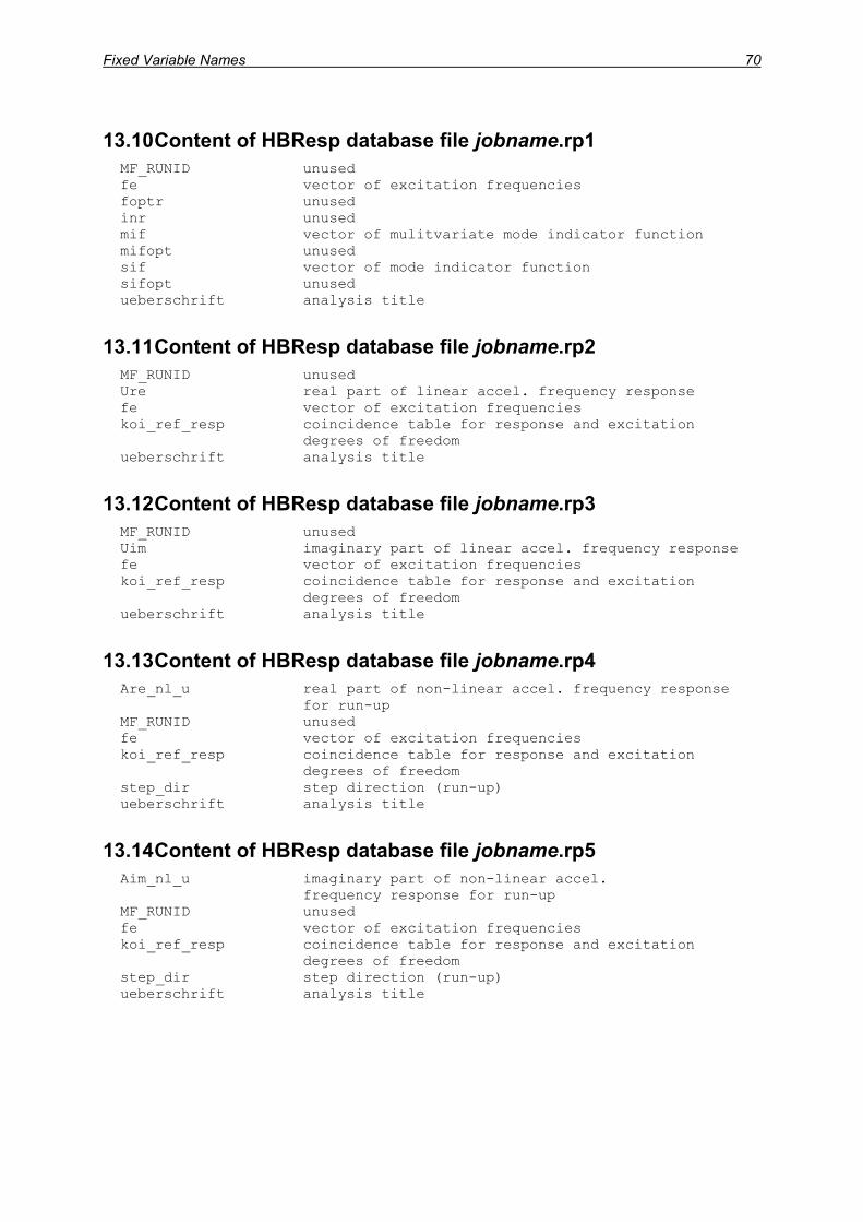
Fixed Variable Names 70
13.10 Content of HBResp database file jobname.rp1 MF_RUNID unused fe vector of excitation frequencies foptr unused inr unused mif vector of mulitvariate mode indicator function mifopt unused sif vector of mode indicator function sifopt unused ueberschrift analysis title
13.11 Content of HBResp database file jobname.rp2 MF_RUNID unused Ure real part of linear accel. frequency response fe vector of excitation frequencies koi_ref_resp coincidence table for response and excitation degrees of freedom ueberschrift analysis title
13.12 Content of HBResp database file jobname.rp3 MF_RUNID unused Uim imaginary part of linear accel. frequency response fe vector of excitation frequencies koi_ref_resp coincidence table for response and excitation degrees of freedom ueberschrift analysis title
13.13 Content of HBResp database file jobname.rp4 Are_nl_u real part of non-linear accel. frequency response for run-up MF_RUNID unused fe vector of excitation frequencies koi_ref_resp coincidence table for response and excitation degrees of freedom step_dir step direction (run-up) ueberschrift analysis title
13.14 Content of HBResp database file jobname.rp5 Aim_nl_u imaginary part of non-linear accel. frequency response for run-up MF_RUNID unused fe vector of excitation frequencies koi_ref_resp coincidence table for response and excitation degrees of freedom step_dir step direction (run-up) ueberschrift analysis title
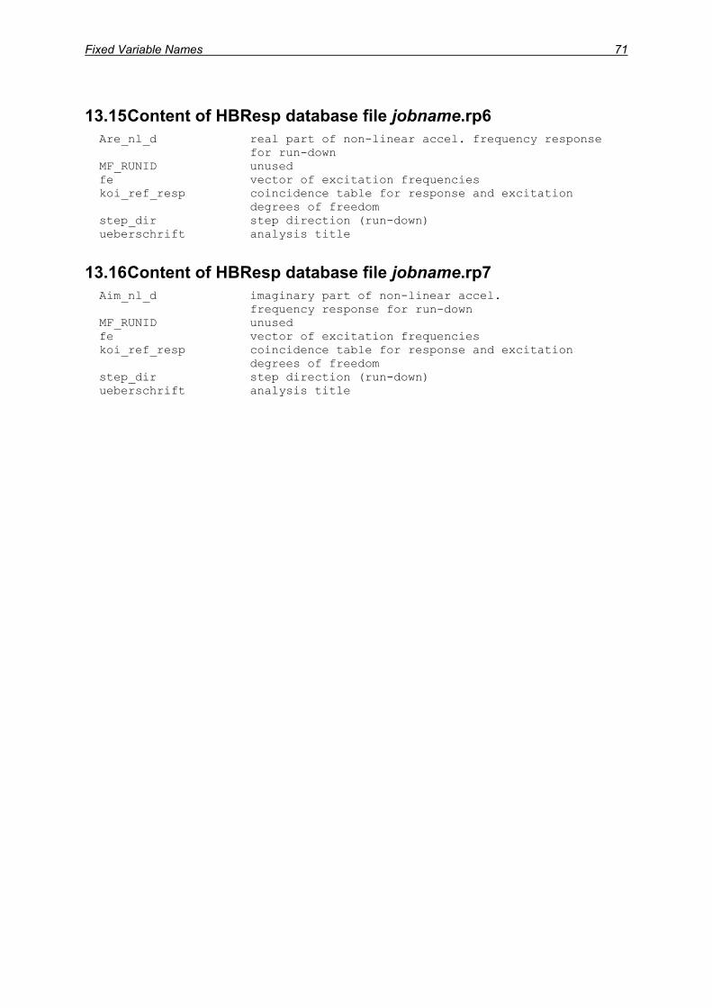
Fixed Variable Names 71
13.15 Content of HBResp database file jobname.rp6 Are_nl_d real part of non-linear accel. frequency response for run-down MF_RUNID unused fe vector of excitation frequencies koi_ref_resp coincidence table for response and excitation degrees of freedom step_dir step direction (run-down) ueberschrift analysis title
13.16 Content of HBResp database file jobname.rp7 Aim_nl_d imaginary part of non-linear accel. frequency response for run-down MF_RUNID unused fe vector of excitation frequencies koi_ref_resp coincidence table for response and excitation degrees of freedom step_dir step direction (run-down) ueberschrift analysis title

Contact 72
14 Contact The harmonic balance response analysis software HBResp has been developed at:
University of Kassel Department of Civil Engineering Lightweight Structures and Structural Mechanics Laboratory
Postal address:
Prof. Dr.-Ing. M. Link University of Kassel Department of Civil Engineering, FB14 Lightweight Structures and Structural Mechanics Laboratory, FGL Moenchebergstr. 7 34109 Kassel - Germany -
E-Mail address:

References 73
15 References [Bathe 96] K.-J. Bathe: Finite Element Procedures, Prentice-Hall, 1996 [Boeswald 02a] M. Boeswald, M. Link: Joint Models Theory and Application
Report, Deliverable D 1.2-1, Report No. CERES.W1.2-UK-XXX, University of Kassel, Lightweight Structures and Structural Mechanics Laboratory, April 2002
[Boeswald 02b] M. Boeswald, S. Meyer, M. Link: Coupling and Reduction
Techniques – Theory and Application, Deliverable D 1.3-1, Report No. CERES.W1.3-UK-001, University of Kassel, Lightweight Structures and Structural Mechanics Laboratory, September 2002
[Boeswald 03] M. Boeswald, M. Link: Update_nl Version 1.0 for HBResp,
User´s Guide, University of Kassel, Lightweight Structures and Structural Mechanics Laboratory, December 2003
[Meyer 01] S. Meyer, M. Weiland, M. Link: Modelling and Updating of Local
Non-Linearities using Frequency Response Residuals, Proc. of the International Conference on Structural System Identification, University of Kassel, September 2001
[Nastran 92] S. H. Lee (Editor): MSC/Nastran Handbook for Non-linear
Analysis, Version 67, The MacNeal-Schwendler Corporation, 1992
[Nastran 94] J.P. Caffrey, J.M. Lee (Editors): MSC.Nastran Linear Static
Analysis User´s Guide, Version 68, The MacNeal-Schwendler Corporation, 1994
[Nastran 01] MSC.Nastran Superelement Analysis, Seminar Notes, Version
2001, March 2001 [Worden 01] K. Worden, G.R. Tomlinson: Nonlinearity in Structural
Dynamics, Detection, Identification and Modelling, Institute of Physics Publishing, 2001