hb, wy go alls
TRANSCRIPT

SIMULATION AND ANALYSIS OF A TIME HOPPING SPREAD SPECTRUM COMMUNICATION SYSTEM
by
Jeffrey B. Mendola
Thesis submitted to the Faculty of the
Virginia Polytechnic Institute and State University
in partial fulfillment of the requirements for the degree of
MASTER OF SCIENCE
in
Electrical Engineering
APPROVED:
- Brian D. Woerner, Chairman
hb, WY go ALLS Charles W. Bostian “ Ivan Howitt
June 12, 1996
Blacksburg, Virginia
Keywords: Spread-Spectrum, Time-Hopping, Ultra-wideband, Multiple Access Communications, Gaussian approximation

LD B55
755 | “| “| oO
M403 ca

SIMULATION AND ANALYSIS OF A TIME HOPPING
SPREAD SPECTRUM COMMUNICATION SYSTEM
by
Jeffrey B. Mendola
Thesis submitted to the Faculty of the
Virginia Polytechnic Institute and State University
in partial fulfillment of the requirements for the degree of
MASTER OF SCIENCE
in
Electrical Engineering
APPROVED:
Brian D. Woerner, Chairman
Charles W. Bostian Ivan Howitt
June 12, 1996
Blacksburg, Virginia
Keywords: Spread-Spectrum, Time-Hopping, Ultra-wideband, Multiple Access Communications, Gaussian approximation
SIMULATION AND ANALYSIS OF A TIME HOPPING SPREAD SPECTRUM COMMUNICATION SYSTEM
by
Jeffrey B. Mendola
Brian D. Woerner. Chairman
Electrical Engineering
(ABSTRACT)
Lately, spread spectrum systems are being increasingly used for commercial wireless
communications because of their ability to reject various types of interference. This ability
allows them to be used in multiple access systems. Direct sequence and frequency
hopping systems have been the primary spread spectrum techniques used in practice. One
technique which has not received much attention until recently is time hopping. In time
hopping, a symbol is transmitted at a random position within the symbol period using a
pulse width which is much smaller than the symbol period. Ultra-wideband (UWB)
technology is a radar technology which shows promise for an relatively simple
implementation of a time hopping system.
This thesis looks at the error probability performance of a UWB time hopping multiple
access system. Previous work has led to an estimate of the performance using a Gaussian
approximation similar to that used for direct sequence systems. Through the use of a fast
simulation technique, it will be shown that in certain situations, the Gaussian
approximation fails to accurately predict the performance. A numerical analysis which
uses characteristic functions is developed and shown to correctly predict the system’s
performance under a wide range of situations. This numerical analysis also contributes to
the understanding of the system.

Acknowledgments
I would like to thank my advisor Dr. Brian Woerner for his help and advise throughout the
research for and preparation of this thesis. I would also like to thank Dr. Ivan Howitt and
Dr. Charles Bostian for their comments on my thesis.
My thanks also go to Robert James for the opportunity to work for the Center for
Transportation Research and to be involved in interesting research.
Finally, I would like to thank my family for their support and encouragement throughout
my studies.
lil

Table of Contents
L. Tmtroduction............ ccc eee cecccseessesnsneececeececeeeceeesseaseseesuqesesssnsssensssessessesesesceseeseeseeseseees 1
1.1. Wireless Spread Spectrum SystemS...........:.ccccseccecessseeenecaceeceeceecesessssssnsseeeees 1 1.2. UWB Time Hopping... eecsecesesssecesesssecesssessecsesesseescesesssneseuseessssaecossaas 2
1.3. Previous WOrKk...........ccccccccccesssssccecessesseecceceessesesacceeceseesessssauaaeasaceeceseseeeeessnaees 5
1.4. Purpose Of ThesiS.......... ces cesseeneeeseesesseeeeeeeceeccsssessesssseeeaessusaaeseseesseeesaaes 6
1.5. Organization Of Thesis... ccccccccccceceeeccceccccenseeeeeesseenssesseesceeeeceeeeaneseeerees 6
2. The UWB PPM Time Hopping System............0....cccccccccccessccececceeeeeeeceeeneeeneeeeeeesesasaas 8
2.1. Structure of the Transmitter. ......0.....cecesssenecesssssceceesseeeeceessssneceeseeeeeeeeeessnas 8
2.2. Channel Model.............ccccsseesseesseesesssecesssnsesecesceecececeaenaauaseseeseeeeceeaueeeaeeseseecs 11
2.3. Structure Of the RECeIVEL.............cccesesnencenecccccceecccceececcesececessccccnansaceseceeeeeess 12
2.4. SUMIMALY........ cece ccceeesseeeecccccscensseesesessceccaseesaesecessseeeeeecaseusaeeseeeuaeesseeeeeanenes 16
3. The Gaussian A pproximation..................cccccccccccccsssesssnseeeseeeceecseceessesseseesseesnanaeeeecs 18
3.1. Using the Gaussian Approximation for the UWB Time Hopping System......18
3.2. Determining the Mean and Variance Of 11y............cesseeseeeeseeeeeseeecceecceceeeeeeeetens 19 3.3. Calculating the Probability Of Error........... ee eeeeeeeeeneececeecceeceeeceseeseeseeaeees 21 3.4, SUMMALY....... ec eeeccccceeseccceeeeeescceascesececaueseeeeueeeeeeaesseeeenseseneaseeceuneeeeuaesseatonss 25
4. Simulation of the UWB PPM Time Hopping System.....0.0.00... cc eeeeeeeeeeteeeeseeees 26
4.1. Purpose of the Simulation............. cc eeeescccccecseeteceeceeeeeceeceeeccceeeseceeseseseaeeses 26
4.2. Simulation Method... ceeessssssseecccacceececeeccecececeseecceseeceescenaneeceeenseaeeess 26
4.3. Simulation Implementation... ccceeseeesscsseeeseeteeceesetesetesesseeeseeeseeneeeeees 29
4.4. Simulation Results......... ce ccecsscccsssescceceecsessessssceeceeeeeseseeseeecseseeecsesnsanaaaaeeees 30
4.5. Summary Of Results..........ceccccccccssessscsseceeeeceeececesceessesesseeeeesseceessesenseseeesens 38
5. A Numerical Analysis of the UWB PPM Time Hopping System................0..00... 39 5.1. Purpose of the Anal ySis.........ceeeesseccceeceessennsnssencecesseceececeeesessceteeeseeseeaeeaeaes 39
5.2. Amalysis Method... ecsssesessssssesceccccececnaenesescceteesensesscceeseuseeeeeseeanaseeeess 39
5.3. Modeling the Characteristic Function Of R.u.ccssssssssssserseterentssaceeeeeneceees 4] 5.4. Computing the Characteristic Function of the Total Receiver Noise............. 43
5.5. Computing the Probability of Error Using Characteristic Functions......... 44
5.6. Comparing the Numerical Analysis with the Simulation Results.................... 45
5.7. Summary Of RESuLts.... ee eeecnecseceeeccecnenecceeeneeessssssesscseeseteceseaseeseneeeees 49
6. Discussion Of Resullts........... ccc cccsscssstecsssteecessneceescneeesessaeeceesssaeecseessaseeessenneeeeseas 53
6.1. Insight Gained From the Numerical AnalySis..............ccccssssccccccessseseseceaeeeeees 53
6.2. A Look at the Convergence of the Gaussian Approximation... 53
6.3. Significance of Important Performance ReSults.............csecccsssssecccssseceessenees 60 7. COMCIUSION. «0.0.0.0... ccc ceesesseceesseseesseessenssssseeeseesceeecescaaauaaasseseeeeeeeaaeaauseeeceeeeaqeaanseess 63
7.1. Summary of Thesis Results............ccssccccssscceccseesssssnecescessessssncsecseesessesesanees 63 7.2. Future Work... cecccccesseeccceceenseseececsensscecaseesceueseceaeeecoaeesceeeeceeeeseeeeaeess 64
8. References... cccessssessececceessesseneeeeseeeessaaeeeesseesecseenssensaaaneesaeseeseeeseeeeseeseesessessees 65
VIA ccc cccsssssneneeceeeeceeceeeeeeceesssssaeeeeeecesesssaseeeeeseeeseseeeeceeeseusaauaaqeneaacaaasgagaasenseeeeeses 67
1V
List of Figures
Figure 2.1 - A plot Of D(t) VS. t/Tin.scccesccccssscccesstscssssssessseesscssaccsseassosaceeesesesessseseessassooaseees 9 Figure 2.2 - Spectrum of the monocycle, p(t), when the pulse width is 1 ns... 10
Figure 2.3 - Transmitter Block Diagram..............scseessssecescssssecesessecsesessseeescessesaaeeseeaas 11
Figure 2.4 - A plot Of W(t) VS. t/Tnssscccsssccccssecccsseccessseceesaeeesseeecsseeseessecesseeeeeesseesesseeeeees 13
Figure 2.5 - Spectrum of w(t) when the pulse width is 1 nS... ee cceecseeeeteeeseneeees 14
Figure 2.6 - A plot of v(f) VS. t/Gin With O/Tn=O.5....eceescceseesseseeeceeseeeesssseseeesesteenseceneenes 15
Figure 2.7 - Spectrum of v(t) when the monocycle pulse width is 1 ns and 8/t,=0.5........ 16
Figure 2.8 - Receiver BlOCK Diagram... cee sseessseeecteeeesseeecesesecssecessneeeeeaeecessaeeeeeeeees 17
Figure 3.1 - Plot of Rw(f)/Ew VS. ttn fOr S=O.STecscecccsscesscsscescensseeessseceseseesseesseesssesaeesss 21 Figure 3.2. - Plot of P. vs. E/N. for different values of N, with N=100........... cc eeeeeee 24
Figure 4.1 - Block diagram for the simulation approach............ees se eeseeecessecceseeeeeeeeeeeeenes 28
Figure 4.2 - Plot of P. vs. E,/N, for different values of N, with N,=6 and T=80.............. 31
Figure 4.3 - Plot of P. vs. E,/N, for different values of N, with N,=6 and N,Tj=480........ 32
Figure 4.4 - Plot of P. vs. E,/N. for different values of N, with N,=6 and N,7/=480........ 33 Figure 4.5 - Plot of P. vs. E,/N, for different values of Np, with N,=11 and N,7/-960......34
Figure 4.6 - Plot of P. vs. E,/N, for different values of N, with N,=11 and N,7—-960......35
Figure 4.7 - Plot of P. vs. N, for different values of T; with N,=1 and F,/N,=20 dB......... 36
Figure 4.8 - Plot of P. vs. P;/P; for different values of N,
with N,=6, NpT7=480, and Ey/No=20 Bu... cee ceseeeseeeeseeeesseeeeteeenneeeenees 37
Figure 5.1 - Plot of the cumulative distribution function Of RyA(T)/Ey......cccsssssssssesteeeeeees 40
Figure 5.2 - Plot of the linear spline approximation to FR(R).........cccsscsccescesssnssnceeseceseeees 42
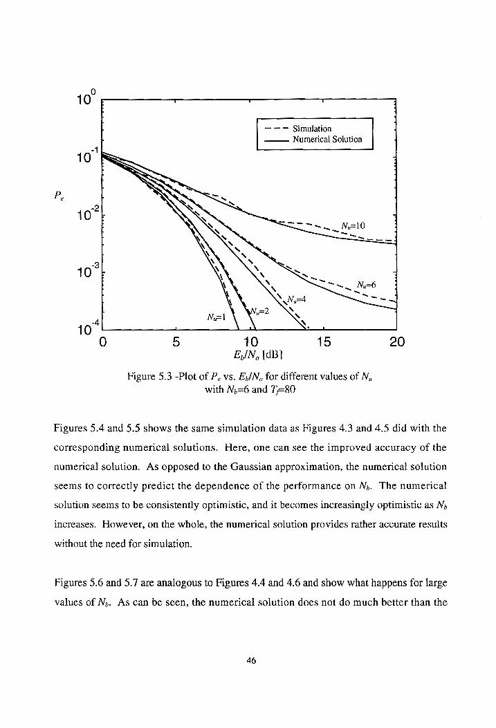
Figure 5.3 -Plot of P. vs. E,/N. for different values of N, with N,=6 and 7)=80............... 46 Figure 5.4 - Plot of P. vs. E,/N, for different values of N, with N,=6 and N,7)=480........ 47
Figure 5.5 - Plot of P. vs. E,/N. for different values of N, with N,=11 and N,7T=960......48
Figure 5.6 - Plot of P. vs. E,/N, for different values of N, with N,=6 and N,7/=480........ 49
Figure 5.7 - Plot of P. vs. E,/N, for different values of N, with N,=11 and N,7/=960......50
Figure 5.8 - Plot of P. vs. N, for different values of 7; with N,=1 and F,/N,=20 dB......... 51 Figure 5.9 - Plot of P. vs. P,/P; for different values of N,
with N,=6, N,7=480, and Ey/No=20 dB... cess ceeesceeeeeeessseceseseecesneerens 52 Figure 6.1 - Plot of P. vs. N, for different values of T; with Ny=1 and Ey/N,=20 dB......... 56
Figure 6.2 - Plot of P. vs. N, for different values of Ty with N,=15 and E,/N,=12 dB.......57
Figure 6.3 - Plot of P. vs. N, for different values of N,7; with N,=15 and E;/N,=20 dB...58

List of Tables
Table 3.1 - Values of E,/m, and E, / m, for various values Of 5/Ty.ccccscsececsesesecccecececees
Table 5.1 - Values of R; used for the linear spline approximation to F(R)........:cccs0cee0es. Table 5.2 - Values used for a; and t; SOS OO SOHO HHEH ERE ESTES EOE EH ETE EEE TELE OEE E EH EEHH OE OOOOH ERES EOE EEHEREEOODECEEOES
v1

1. Introduction
1.1. Wireless Spread Spectrum Systems
There has been a surge of interest in spread spectrum communications, especially for non-
military applications. Military systems use spread spectrum for covert communications
and their resistance to jamming. On the other hand, cellular phone networks and other
wireless radio applications benefit from using spread spectrum systems because of their
interference rejection capabilities. This interference rejection provides resistance to
multipath fading. It also helps to reject narrowband interference which can allow these
systems to be overlaid over existing narrowband channels. Most importantly, spread
spectrum signals can reject other users’ signals and this allows them to be used in a Code
Division Multiple Access (CDMA) system. CDMA systems have the interesting property
that the system performance degrades gracefully with increases in the number of users.
Currently, the two spread spectrum methods which are used in practice are direct
sequence (DS) and frequency hopping (FH). In direct sequence, the binary data is
multiplied by a binary, pseudo-random spreading sequence whose symbol rate is much
higher than the data rate. Correlation with the pseudo-random spreading sequence
provides the interference rejection. Right now, DS spread spectrum is the method which
is used most often in practice. Currently, it is used in the IS-95 cellular radio standard, in
unlicensed “Part 15" devices like cordless telephones, and in the Global Positioning
System (GPS) which is a satellite positioning system.
In frequency hopping, the center frequency of the transmitter is changed in a pseudo-
random manner. Interference rejection is obtained when the mterference is narrowband
because the transmitter will not always be transmitting on the frequency that the
interference occupies. A slow frequency hopping system has a hopping rate (the rate at
which the center frequency changes) which is slower than the data rate, and a fast
frequency hopping system has a hopping rate which is faster than the data rate. Fast

frequency hopping provides diversity since each data bit is transmitted more than once, but
it demands very stringent synchronization requirements. For this reason, most of today’s
systems use slow frequency hopping. Frequency hopping is employed in the GSM cellular
radio standard to provide immunity to fading, and it is also used in Cellular Digital Packet
Data (CDPD).
One method which until recently has received very little attention is called time hopping
(TH). As one might guess, time hopping can be thought of as a dual of the frequency
hopping method. In frequency hopping, the total transmission bandwidth is divided into
many smaller channels, and then each user regularly switches which channel it uses in a
pseudo-random manner. In time hopping, the bit period is divided into small time intervals
with each user regularly switching the interval it uses in a pseudo-random manner. On the
other hand, time hopping can also be thought of as a low duty cycle, time-varying version
of direct sequence spread spectrum. The bandwidth spreading, which is common to all
spread spectrum signals, is achieved by having each user only transmit for a small fraction
of the bit period.
1.2, UWB Time Hopping
Time hopping has received little attention until recently. This because it has more stringent
timing requirements than DS or FH and because in general the receiver is more complex
than for the other methods. However, some recent developments have led to a technology
which shows promise for relatively simple and low cost implementation of a time hopping
system. This technology which is known as ultra-wideband technology and has grown out
of the radar field. Ultra-wideband (UWB) technology was developed for radars for the
purpose of getting fine resolution on range measurements. UWB technology basically
uses signals with such large bandwidths that they can no longer be considered as
conventional RF signals. These signals are characterized by their bandwidth to center
frequency ratios. Narrowband systems have ratios less than 0.01, and conventional

wideband systems (such as other spread spectrum systems) will have ratios which are
usually less than 0.25. UWB signals, however, have ratios in the range of 0.25 to 2.0. In
a sense, these signals are really just baseband pulses of electromagnetic energy. Because
of this, UWB technology is sometimes known as non-sinusoidal or impulse technology.
As can be seen, UWB signals are very different from the conventional signals normally
used in communication systems. This fact has lead to some obstacles in the development
of practical UWB systems. One obvious challenge is to develop transmitter circuitry
which is able to transmit short duration pulses. However, there are currently devices
being developed by a few companies which have sufficiently short pulses. Prototypes with
pulses on the order of nanoseconds have been developed and tested. Another challenge in
implementing UWB devices is developing devices which can transmit high powers. This is
especially the case when the device is to be used in a long range radar system. Because
UWB signals have low duty cycles, the devices must be able to handle much higher peak
powers than those normal seen in conventional systems. The antenna used in an UWB
system must also receive special attention. Since UWB signals are not narrowband
signals, specially designed antennas must be used in order to get the normally desired
directivity. The problems with high powers and directive antennas are currently being
researched. However, applications which can tolerate omni-directional antennas and
which operate with small powers (and thus small ranges) can use UWB technology
without having very complex or costly systems.
Currently, there are a few companies which are in the process of developing devices which
can be manufactured with solid state technology. These devices also use very low
transmitted power levels and low gain antennas. One of the companies is Aether Wire and
Location, Inc. of Nicasio, California which is developing UWB devices which can perform
accurate location. They are very close to coming out with a commercial product. Pulson
Communications is developing UWB technology for a time hopping multiple access

communication system [1]. Lawrence Livermore Laboratories has also developed their
own UWB technology and is now licensing this technology for various applications [2].
As mentioned above, UWB signals can be used in a time hopping system. Pulson
Communications is working on a time hopping system described in [1] which R. A.
Scholtz has and analyzed in [3,4]. The basic signal is a pulse train of UWB pulses (called
monocycles because they resemble one cycle of a sine wave) where the pulse widths are
on the order of a nanosecond and the pulse repetition frequency is on the order of a
megahertz. The interval between pulses is then varied by a pseudo-random code. This
can be visualized as having each monocycle being “hopped” to different positions within
each pulse repetition interval, or frame. The monocycle positions are then slightly shifted
again in order to modulate the signal with the information sequence. Thus, this system
uses a pulse position modulation (PPM) scheme. This system can support multiple access
communications by having each user transmit with its own pseudo-random hopping
sequence. As mentioned before, this system can be thought of as the dual of a frequency
hopping system. However, the hopping rate is not limited as much as it is in a frequency
hopping system, and thus, fast time hopping systems are practical. This allows the system
to take advantage of the diversity that fast hopping provides.
UWB signals have some interesting characteristics with are worth mentioning. As with all
spread spectrum systems, time hopping systems are able to reject many types of
interference. UWB signals are different in that the small pulse widths allow the system to
reject (or resolve) multipath components with much smaller path differences than other
spread spectrum systems. The small pulse widths also give the system very accurate
location information. This allows for a system which can both track and communicate
with a mobile receiver. Researchers at the Virginia Tech Center for Transportation
Research are examining the application of UWB technology to Intelligent Transportation
Systems [5]. One example is an Automated Highway System where communication links
allow processors on the roadside to completely control every vehicle on a highway. It is
believed that UWB devices can locate each vehicle with accuracy on the order of
centimeters and provide the communication link so that the processors can control the
vehicles.
One important consideration is how UWB signals, which have such enormous bandwidths,
are going to affect existing narrowband signals. Fortunately, UWB signals have some
characteristics which permit them to be overlaid over existing narrowband users. The
pseudo-random hopping is very important even in systems without multiple access
capabilities because it “spreads” the energy of the signal over the entire bandwidth
occupied by a signal pulse. This means that the power spectral density would be much
lower than narrowband signals with the same power. Another important point is that
UWB signals have very low duty cycles. Finally, current UWB devices are being
developed for short range applications and thus have transmitter powers of 100 uW or
less. All these facts indicate that UWB systems may cause negligible interference to
narrowband users and can be overlaid over them. In fact, contacts at the FCC say that in
the near future Part 15 Specifications might be changed to include UWB devices with
power limitations. [6] Because of these spectrum issues, it is apparent that UWB devices
will never be used for large scale systems. However, for specialized systems, UWB is an
emerging technology which is practical and has attractive features.
1.3. Previous Work
As mentioned before, there has not been much research into TH spread spectrum systems.
A few researchers like Lam and Sarwate [7] have looked at time hopping multiple access
packet communications. A general description of the UWB system is presented in a paper
by Withington and Fullerton [1]. The papers by Scholtz [3,4] present an analysis of the
UWB system using a Gaussian approximation. Since TH can be thought of as the dual of
FH, there are some papers on FH which help to provide insight into the performance of

TH systems. In a paper by Wang and Moeneclaey [8], a fast FH system in a fading
channel is analyzed. The paper by Geraniotis [9] presents an accurate analysis of a FH
system using characteristic functions.
1.4. Purpose of Thesis
As mentioned before, the UWB time hopping PPM system was studied in papers by
Scholtz [3,4]. In these papers, the BER performance of the system is analyzed by using a
Gaussian approximation that is very similar to the one used for DS spread spectrum [10].
This analysis yields a very compact result which resembles the result for DS. The purpose
of this thesis is to examine the Gaussian approximation presented by Scholtz. Through the
use of a novel simulation technique, the Gaussian approximation will be investigated to see
how well it applies in certain situations. It will be shown that in certain significant cases,
the Gaussian approximation is quite optimistic. An alternative performance evaluation
method based on integration of the characteristic function is developed and shown to be
more accurate over a wide range of examples. This technique contributes to the
understanding of UWB time hopping systems.
1.5. Organization of Thesis
The rest of the thesis will be organized in the following manner. Chapter 2 provides a
detailed description of the transmitter and receiver. This will allow for a derivation of the
Gaussian approximation in Chapter 3 using a slightly simpler approach than used in [3,4].
Next the simulation method and results will be presented in Chapter 4. These results will
show where the Gaussian approximation fails to accurately predict performance. Then, a
more accurate analysis using characteristic functions will be presented in Chapter 5. This
analysis will also provide some insight into the system and help to explain why the
Gaussian approximation fails in certain circumstances. In Chapter 6, reasons why the
Gaussian approximation fails will be discussed along with some of the practical
implications of the results which were presented throughout the thesis. Finally, a summary

of the results of this thesis and some future research directions will be discussed in
Chapter 7.

2. The UWB PPM Time Hopping System
In this chapter, a mathematical model for a time hopping multiple access system which will
be used throughout the remainder of this thesis will be introduced. As mentioned before,
the UWB PPM time hopping system was described and analyzed using the Gaussian
approximation in [3,4]. Thus, most of the discussion of the system and the Gaussian
approximation, except when explicitly stated, is based on the model from [3,4].
2.1. Structure of the Transmitter
The signal transmitted by the k’ user, s,(t), in the UWB time hopping multiple access
system is given by
s,(t)= ¥ p(t iT, - ¢}T, ~ 8d), )) (2.1)
where p(f) is the pulse shape of the transmitted monocycles. The transmitted pulses are
called Gaussian monocycles because they resemble smoothed single cycles of a sine wave.
Figure 2.1 shows a plot of the pulse shape, p(t). As one can see from (2.1), the
transmitted signal is a pulse train with each pulse beig shifted in time by a different
amount. The i7; term separates each monocycle by 7;, the nominal pulse repetition period,
or frame period.
The c\’T, term adds the pseudo-random time hop to each monocycle. The pseudo-
random code for the i” monocycle transmitted by the k” user is specified by c which is
a pseudo-random integer on the interval [0, N,]. The variable 7, specifies the resolution of
the time hops. This time hopping term has several important purposes. First of all, the
code provides the interference rejection capability for the system. At the receiver,
interference will be rejected because the code will make the interference uncorrelated with
the user’s signal. When interference rejection is not required (e.g., the system does not
require CDMA), the time hopping code is still important. Without it, the user’s signal is
basically a modulated pulse train with regular intervals between the pulses. The spectrum

0.15
0.1
0.05
PO g
-0.05
-0.1
-0.15
-0.5 0 0.5 1 1.5 2 2.5 thtm
Figure 2.1 - A plot of p(r) vs. Tn
of this signal will be a train of narrowband spikes which will cause significant interference
to the narrowband systems which already exist in these bands. The hopping code
randomizes the intervals between pulses which causes the energy of the signal to be spread
evenly throughout the bandwidth that an individual pulse occupies. Figure 2.2 shows a
plot the spectrum of an individual pulse when the pulse width is 1 ns. As can be seen, the
bandwidth of the pulse is a few GHz. Thus, the hopping code ensures that the signal will
have a large bandwidth and low power spectral density. With the hopping code, the signal
is SO wideband that it may be considered a baseband signal.
The term Sdn, | adds the modulation to each monocycle where qin, , is the data bit (0
or 1) which modulates the i” monocycle of the kK" user. Thus, no additional shift is

2 3
f [GHz]
Figure 2.2 - Spectrum of the monocycle, p(?),
when the pulse width is 1 ns
applied when the data bit is a 0, and a shift of 5 is applied when the data bit is a 1. As can
be seen, this system uses PPM to encode the pulse train with the data stream. The term
Lin, J represents the index of the data bit where L-] is the floor function. This means that
N, monocycles will be modulated by the same data bit, and thus, this system is a fast time
hopping system.
In order to keep monocycles from hopping into frames other than their own, the
parameters of the hopping code must satisfy
N,T, ST, -T,,—-5 (2.2)
where 7, is the width of the monocycle pulse. Also it is easy to show that the bit rate, R,,
10

is given by
R,=——. N,T, (2.3)
Figure 2.3 shows a block diagram of the transmitter (which is based upon a figure from
[3,4]).
s(t) Pulse generator -————>
Output
. (k) (k Y8(t-i7, - cf 7, - 84%, 1) dy”
——— >| Modulation shift Input
. (k) data n > S(t —iT, ~¢; T.)
Code generator Code shift
>i5(t-i7;)
Frame clock
Figure 2.3 - Transmitter Block Diagram
2.2. Channel Model
The channel model used throughout this thesis will be very simple. It will be assumed that
the channel causes non-varying attenuation and delay to each user’s signal and that the
received signal, r(f), is corrupted by additive white Gaussian noise (AWGN), n(t). This
simple channel model will help to keep the analyses performed in this thesis simple.
However, this simple AWGN channel model is not that far from reality. There are
indications that multipath and Doppler effects will not have as severe an impact on
performance as they do in narrowband systems. In fact, the Rayleigh fading which is
common in mobile communications only happens with narrowband systems and will not
11

affect UWB systems [1]. Instead, the Doppler shift will cause the time features of the
signal to be expanded or contracted, and the amount of this fluctuation is insignificant
even at very large speeds [11]. The only effect which could possibly be significant is the
fluctuation of the frame period, but the fluctuations would be small enough to be corrected
by a tracking loop. Multipath will not be a big problem since the short pulse width of the
system will also cause all but the shortest path differences to become uncorrelated with the
original signal. The only potential problem is that the signal power might become so
spread out between the multipath components that the performance will be degraded
significantly. Solving this problem by using a RAKE receiver might in itself cause more
problems. This is because the very small time resolution might make the receiver very
complex [3]. This small time resolution also makes the synchronization process more
complicated [3].
2.3. Structure of the Receiver
At the receiver, the signal, r(t), due to N, users and additive white Gaussian noise, n(f), is
given by
N,
r(t)= Yi VPA (t)+n(t) (2.4) k=l
where
rth= ¥ w(t-t, -iT, —cT, ~ 8d5n,\)- (2.5)
In (2.4) and (2.5), Px is the relative received power of the kK" user’s signal, and T, is the
relative time delay of the k* user’s signal. In (2.5), w(t) is used as the received
monocycle’s pulse shape. The reason why this is not p(t) is because the monocycles are
baseband pulses, and thus, their shape is affected by both the transmitting and receiving
antennas as well as the channel itself. All antennas have some frequency dependence
which will affect a signal. For narrowband signals, this dependence will not affect the
signal; however, for wideband signals, the pulse shape will be altered. For the antennas
12

normally used in UWB systems, w(t) is approximately the time derivative of p(t). Thus,
r,{t) is approximately the time derivative of a shifted version of s(t). When the
monocycles are received, their shape is given by
we+T,/2)=[1—4n(1/c,,) Jenn? (2.6)
where T,, is a constant which determines the width of the pulse. The term 7,,/2 is just used
to shift the pulse so that the it begins at =O. Figure 2.4 shows a plot of w(t). As can be
seen from this plot, 7, is approximately 2.5t,,. Figure 2.5 shows a plot of the spectrum of
w(t).
It is assumed that the receiver has both time and code synchronization with the user’s
signal which it wishes to demodulate. Thus, the receiver can generate replicas of the two
w(t)
tltm
Figure 2.4 - A plot of w() vs. Tn
13

3
f(GHz]
Figure 2.5 - Spectrum of w(t) when the pulse width is 1 ns
possible signals which it can use in a correlation receiver. This is the optimum receiver for
that user’s signal assuming only AWGN is present. This decision rule is as follows:
1, +T, (I41)N,-1
decide di? =O if | r(t) Sy wt-t, -iT, -c Tat } i=IN,
1, +7, (I41)N,-1
> | rt) Swe-t, -iT, eT, -8)at. (2.7) T, i=IN,
By rearranging (2.7), an equivalent but simpler decision rule is given by
. (I41)N,-1
decide df? =0 if Z” = Vz" >0 (2.8) i=IN,
where
14

260 = fe yy —t, -iT, ~ oT Dat 2.9) t,4T,
v(t) = w(t)-wt-8). (2.10)
Hence, only one decision statistic is needed, and this statistic is obtained by summing the
correlations of each monocycle with the template signal v(t). Figure 2.6 shows a plot of
v(t) when 6/t,=0.5. In the next chapter, it will be shown that this value of 5/t, is close to
the choice which gives the optimal performance. Figure 2.7 shows the spectrum of v(t).
By looking at Figure 2.6, one can see how the template signal will work. When the
transmitted data bit is a zero (no shift), then the main lobe of w(4) will line up with the
large positive peak of v(t) and the resulting correlation will have a large positive value.
When the transmitted data bit is a one (a shift of 5), the main lobe of w(2) will line up with
1.5
-1.5
tlm
Figure 2.6 - A plot of v(2) vs. t/tm with 5/t,=0.5
15

‘ a i i
0 1 2 3 4 f [GHz]
Figure 2.7 - Spectrum of v(t) when the monocycle pulse width
is 1 ns and &/T,,=0.5
the large negative peak of v(t). The correlation of this signal with v(t) will result in a large
negative value.
As with other spread spectrum systems, this receiver is not optimal if the other user’s
codes are known, but it has good performance and is not very complex. Figure 2.8 shows
the block diagram of the receiver taken from [3,4].
2.4. Summary
In this chapter, a simple model for the UWB time hopping system has been presented. In
the next chapter, a simple analytical result will be developed for this model using a
16

Gaussian approximation.
() a 21" | Threshotd |_4*” r i | Correlator > roe Ae detec vot >
Input integrato Output
> -(t-t, - iT, oT.) data
Template
generator
> 5-1. - iT, - eT.)
cf! Code shift Code generator
> 5(t-t. -iT;)
Frame clock
Figure 2.8 - Receiver Block Diagram
17

3. The Gaussian Approximation
3.1. Using the Gaussian Approximation for the UWB Time Hopping System
As with other spread spectrum systems, a good estimate of the bit error probability for the
UWB system can be obtained by assuming the total noise seen at the receiver is Gaussian.
This is normally a good approximation when the multiple access interference can be
modeled as a sum of a large number of independent random variables. Thus, the noise is
approximately Gaussian by the Central Limit Theorem (CLT). In this analysis, it will be
assumed that user 1’s signal is the desired signal and that the receiver is trying to
demodulate a‘, the 0” bit. Thus, the decision statistic, Z, for the receiver will be
given by
Z =m+n, (3.1)
where m is the constant part due to the signal and n, is random noise. The values of m
when d‘? =1 and when d(” =0 are given by
Np~l +6 +1)T
m= >] [Pw t-1, -iT, - PT, -8)vt-1, iT, — PT at (3.2) i=Q
THT,
Nowl oa 4G4 mM, = J OO" [Rw(t-t, -iT, eT vt—t, -iT, — cP Tat (3.3)
A SH, 1 pep TG Ae TAA NE ACI?
respectively. By rearranging some terms and performing some variable substitutions, mm;
and mp can be simplified to
M =—-mM, = VPN,m, (3.4)
where
m, = | w(t)v(t)dt = E, - R,) (3.5)
and
E,, =3Tm (3.6)
R,(t) = { weep —t)dt = E,[4n°(t/t,.) —4n(t/t,,) + 1fe*-) . @.7)
18

In (3.5), (3.6), and (3.7) E, denotes the energy of the monocycle waveform w(f), and
R,(7) is its autocorrelation function. The random noise, n,, is given by
Nort ne agenr|
n= Dy cer [ve ona poem ~iT, — eT, de. (3.8)
Now, in order to use the Gaussian approximation, the mean and variance of n, (U, and 07)
must be determined.
3.2. Determining the Mean and Variance of n,
In order to find o? and u,, Sholtz [3,4] uses (3.8) directly and some limiting assumptions
on size of N,T.. However, a simpler method which requires fewer assumptions can be
used. First (3.8) is simplified as follows:
N, N,-1 N,
n, =n, +n, = Sy yi ni? + S [n(t+t, +iT, + CT, \v(t)dt (3.9) k=2 i=0 i=0 —20
where ny is the noise due to multiple access interference and n, is the noise due to the
AWGN in the channel. In n;,, the random variable n\ is the interference in the i”
monocycle due to the k” user. Because n(t) is zero mean AWGN, the mean and variance
of n, are given by [12]
u, =0 (3.10)
oo = wes {var = “eee, —2R,,(5)]= N,N, (3.11) oo
where N, is the one-sided power spectral density of n(f). Assuming the n“’s are i
independent (as is done in [3,4]), then the mean and variance of n; are given by [12]
N, N,-1
Lb, =>) dvi (3.12) k=2 ix0
N, N,-1 o7=> Yo? (3.13)
k=2 i=0
where [l,, and 67, are the mean and variance of n{“ respectively.
19

Since n{ is due to "hits" (i.e., when a monocycle overlaps with the correlator’s template
function), then an appropriate model of n{ is given by
R ; ; n®) = VP. w(t), given a hit occurs (3.14)
O, given no hit occurs
where
R,,(t) = | w(t-t)v(t)dt = R,(t)- R(t -8) (3.15)
and T is a random variable which denotes the offset between the interfering monocycle and
the template function. In this model, tis assumed to be uniformly distributed on the
interval where R,,(t) is non-zero. This interval is denoted as Tr and is approximately 4t,,
when 6 is 0.51, (See Figure 3.1). The final piece of information needed is, P,, the
probability of a hit. Assuming each monocycle’s position is uniformly distributed over the
frame interval, the probability of a hit is given by
p= 28, (3.16) T,
Thus, the mean and variance of n‘“? are given by [12]
PP, 7 Ws, _ Pid J R,, (Ade = 0 (3.17)
Tr —0o
o?, = fof J 2, (at = Timi ahh (3.18) a el
where
E, = fr (ar= Ey [10s ~(105-420n(8/t,.) +210n?(8/t,,) To 722 ™
-28n3(5/t,,)° +n*(/t,) Jer” | (3.19)
20

-D — — -3 -2 -1 0 1 2 3
ttm
Figure 3.1 - Plot of Ru (t)/Ew vs. ttm for 5=0.5Tm
Thus, , is a zero mean random variable with variance, 07, given by
“. It _ FE o3=MNm, +0) mR (3.20) k=2 T;
3.3. Calculating the Probability of Error
If probability of transmitting a "1" or a "O" are both equal to 1/2, then, using the Gaussian
approximation, the bit error probability, P., can be calculated using
P,=1+P(m+n, < Olas” =0)+4P(m+n, > Olas” =1)
21

5% }.Fof | = of | (3.21) O0,)/ 2 \o, oO,
O(x) = = { et Pat. (3.22)
where
Putting everything together gives
VPN pt, 1
P=O ——F =Q = mp (3.23)
N,N,m, + mee R 2S P, Fw No 4 tm ay Ty i m, E, N,T, m, im F,
where E;, is the energy per bit and is given by
E,=P.N,E,. (3.24)
The terms £,/m, and E, / m, in (3.23) depend only on 6/t,,, and, thus, a value for 6 which
minimizes P, can be found. The term E,/m, is the reciprocal of the normalized signal
amplitude at the output of the correlator, and the term E, / m, is the ratio at the output of
the correlator of the normalized power caused by a hit to the normalized signal power.
Not only do these factors depend on 6/t,,, but they will also change if a different pulse
shape is used. In Table 3.1 below are some values of E,/m, and E,/ m, for different
values of tn. The first two rows show the values when E,/m, and E, im; are
minimized respectively. Thus, the first row values would minimize P, when the channel
noise is dominant, while the values in the second row would minimize P, when the
multiple access interference is dominant. However, as Table 3.1 shows, the values from
the first two rows are relatively close together. Since the multiple access interference is
normally dominant, the values in the second row are more appropriate. However, in order
22

to simplify the simulation which will be presented in Chapter 4, a value of 5/t,, equal to
0.5 will be used throughout this thesis. Table 3.1 shows that this choice does not alter the
results significantly.
Table 3.1 - Values of E,/m, and E, /m) for various values of 8/T,
Von E,/mp E R / m,
0.5408 | 1/1.618 | 0.68896
0.5022 | 1/1.603 | 0.68265
0.5 1/1.601 | 0.68267
Substituting these values into (3.23) gives the following:
j P=Q (3.25)
joes N,_, 0683
0683¢,, ee P, 16E, NT, in®
Despite the difference in notation, this results from (3.23) and (3.25) are the same as those
in [3,4]. However the approach used here uses fewer assumptions and is slightly less
complex. Also, parts of the result from [3,4] were done numerically and thus do not
explicitly show the dependence on 6 and Tn.
The results of the Gaussian approximation for time hopping look very much like those for
DS/SS. If the fact that T,, is approximately 2.51,, is used, then (3.25) can be rewritten as
1 P.=Q =
N, , 1 yA 16E, 37N&P
(3.26)
23

where N is the processing gain and is given by
_ Nol po m
N (3.27)
This result is exactly the same as the result for DS except for the two numerical constants.
The 1.6 is a 2 for DS and shows that DS is better when the channel noise is dominant
because it uses antipodal signaling. The 3.7 is a 3 for DS and shows that the UWB time
hopping system is slightly better at rejecting multiple access interference. This is a crude
comparison, however, because the results for DS are for rectangular pulse shaping which
is not possible in the UWB system.
Figure 3.2 shows a plot of the Gaussian approximation from (3.26) for various values of
N, with N=100 and all P,’s equal to P;. This plot is similar to plots used to show the
0
10 7
10"
10°} ; N,=50
P, | 3
10 : N,=30 3
10° . 90 : N.=10 -
N,=1
10° — - 0 5 10 15 20
E,/N, (dB)
Figure 3.2 - Plot of P. vs. E,/N, for different values of N, with N=100
24

performance of DS/SS systems and shows how the performance changes as the number of
users increases.
3.4. Summary
In this chapter, a Gaussian approximation has been used to estimate the performance of
the UWB time hopping system. This has led to an analytical result which is rather simple.
In the next chapter, a simulation of the UWB time hopping system will be used to see how
well the Gaussian approximation predicts performance in various situations.
25

4. Simulation of the UWB PPM Time Hopping System
4.1. Purpose of the Simulation
When one has analytical results for the performance of a communication system, then it is
fair to ask why simulation results are needed. A typical answer would be that they are
needed to verify the analytical results. For the case of the UWB/TH system, this answer is
justified because the analytical results are based upon assumptions and approximations.
This is not to say that some of the assumptions are possibly unwarranted, but sometimes
assumptions will only apply in certain idealized circumstances. Thus, by showing under
what circumstances the analysis is valid, simulation can provide valuable insight into the
system performance.
For the UWB/TH system specifically, there are indications that the Gaussian
approximation might not be valid under some circumstances. The CLT applies for all but
pathological distributions (e.g. distributions with infinite moments); however, it will not
apply if the random variables being summed are dependent. Thus, if some of the
assumptions on independence are not valid, then the Gaussian approximation could
provide incorrect results. This problem is seen in the Gaussian approximation of the
performance of DS/SS. Some papers [13,14] have shown that the Gaussian
approximation is optimistic in certain situations because the multiple access interference is
dependent on the desired user’s spreading sequence. Another important consideration 1s
that the CLT only guarantees convergence and does not specify how the convergence
rates vary between distributions. Because the statistics of the multiple access interference
for UWB/TH system are complicated, there is a chance that characteristics of the true
distribution will affect the convergence in certain situations.
4.2. Simulation Method
The usual approach to simulation of communication systems is to find a suitable sampling
frequency and represent the signals in digital form. If the RF signals are being simulated,
26
then the complex envelope representation can be used to transform these signals into
baseband equivalents. The system is simulated by sequentially processing the digital signal
using mathematical models for each component of the system. A Monte Carlo BER
simulation would then, using the correct decision rule, decide upon the received sequence
of bits and calculate the number of errors that occurred in the decision process. This
approach leads to very long simulations for spread spectrum systems because of their large
bandwidth. However, with the UWB/TH system, the low duty cycle means that the
information content of the signal is contained is small periods of time. Thus, much of the
generated digital signal is not used to determine performance. The UWB/TH system also
does not fit into the normal simulation strategy because it uses wideband signals. Thus,
the complex envelope representation is not appropriate because it can only be used for
narrowband signals.
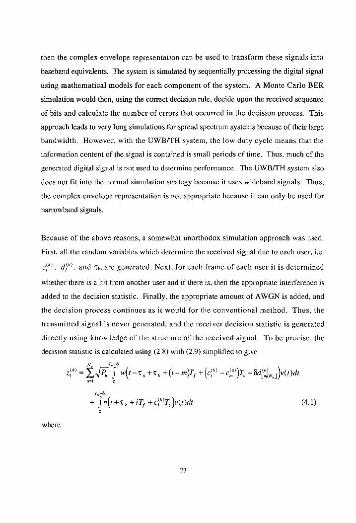
Because of the above reasons, a somewhat unorthodox simulation approach was used.
First, all the random variables which determine the received signal due to each user, i.e.
(x) i co, d, and %, are generated. Next, for each frame of each user it is determined
whether there is a hit from another user and if there is, then the appropriate interference is
added to the decision statistic. Finally, the appropriate amount of AWGN is added, and
the decision process continues as it would for the conventional method. Thus, the
transmitted signal is never generated, and the receiver decision Statistic is generated
directly using knowledge of the structure of the received signal. To be precise, the
decision statistic is calculated using (2.8) with (2.9) simplified to give
N, Ty
zi) = Lv | w(t—t, +1, +(i-m)I, + (ci — cf VT, — 8a", v(t)at “= 0
T,,+5
+ [n(t+e, +iT, +cT, v(t)de (4.1) 0
where
27

m=| (iT, —T,+T, +cT. /T, |, (4.2)
When it needs to be determined whether or not a hit occurs, the simulation just needs to
check if the argument of w() in (4.1) is in the interval [0,T7,,]. Also, since the signals are
digitized, the integrals in (4.1) are simply computed using sums. Figure 4.1 shows a
general block diagram of the simulation approach used here.
Generate random samples
(k) Ck) of & 54 andy
Determine whether or not a hit ch) ge
occurs using “i , “! ,and %%
If a hit occurs add appropriate amount of Repeat for
interference N, frames
Add appropriate
ammount of AWGN
Make the bit decision Repeat for the
and determine if an error > required number
occurred of bits
Figure 4.1 - Block diagram for the simulation approach
This method reduces the simulation time significantly, and it also makes the run time
relatively independent of 7; The drawback of this approach is that it is very specialized to
the particular system configuration and channel model. Slightly more sophisticated
channel models would be nearly impossible to incorporate into this method. Also, because
this method is not modular, any changes the system or channel models require wholesale
changes to the simulation code.
28

4.3. Simulation Implementation
The first thing that must be specified in this simulation is the structure of the signals. Even
though the transmitter and channel will not be explicitly implemented, the signal structure
needs to be known in order to construct the received signal in the receiver. As with all
communication system simulations, only changes in the relative time scaling will affect the
results. Thus, one particular absolute scaling can be simulated, and the results can be
applied to other systems with similar relative scaling. In these simulations, the time was
scaled so that the sampling frequency was equal to | sample/s. In order, to get a relatively
fine time resolution, the width of the received monocycle pulse, T,, was set equal to 25
samples. This choice will not significantly increase the simulation time because the
simulation time will be approximately independent of 7; Because T,, is approximately
2.5Tm Tm WaS set equal to 10 samples. Because the smallest time shift possible is 1
sample, 5 must be an integer multiple number of samples. A value of 5/t,, equal to 0.5
makes this constraint easy to satisfy, and thus, 5 was set equal to 5 samples. This is why
the value of 8/t,, was set equal to 0.5 in Chapter 3.
As mentioned above, there are no distinct modules which implement the transmitter and
channel. However, the parameters which describe them (d{“’,c, %, and n(¢)) must be
specified. Since d{”? is the bit stream for each user, it is generated using a binary random
variable with the probability of a one or zero being equal. As mentioned in Chapter 2,
ci} I
is a random integer uniform on [0, N,], and in order to get the largest number of
hopping positions, 7, is set equal to 1 sample. Then using (2.2), the maximum possible
value of N, is chosen. Since offsets between users can only determined to the nearest bit,
the t’s will be generated using a random integer uniform on [0, N71] where N,7;1is in
terms of the number of samples. The channel noise n(t) is AWGN so that its samples are
generated using independent, zero mean Gaussian random variables. The variance of
29

these random variables is determined from the value of E,/N, being simulated. For
discrete samples of an AWGN process, the variance of the noise is given by [15]
2_N.f,
2 o (4.3)
where f; is the sampling frequency and N, is the one-sided power spectral density. Using
(3.24) and the fact that f, is 1 sample/s, (4.3) can be rewritten as
2 _ 3t ,N,
16E,/N, (4.4)
To prevent the simulation from only examining one fixed case, each user’s bit stream is
divided into small blocks with new 1;,’s being generated for each block. The number of bits
per block per user for which decision statistics are generated will be 2 less than the
number of bits in a block. The two unused bits will be the first and last bits in the block,
and they are only used to simulate interference for other users. Many of the simulations
were run for the case of equal powers for all users. The simulation times for these cases
were reduced significantly by determining the bit errors for all the users rather than one
particular user. Also, all the simulations were run for a fixed number of errors rather than
a fixed number of bits. Again, this decreases the simulation time by only simulating the
number of bits which are needed to get a desired accuracy. The error limit for all
simulations was set to 100 errors. This value leads to BER results which are at most off
by a factor of 1.3 (with a 99% confidence interval) [15].
4.4, Simulation Results
In the following simulation results, systems with N,7; equal to 480 and 960 samples were
used. These values were chosen because they have a large number of integer factors.
Thus, many different systems with the same processing gain but different values of N, can
be simulated. The value of processing gain for these systems is less than the values that
are being proposed for practical systems. However the results seen here can be easily
30

extended to systems with different processing gains.
The first set of results is shown in Figure 4.2. This is a plot of P. vs. E,/N, for different
values of N, with N,=6 and T=80. This type of plot is commonly seen in discussions on
other type of spread spectrum because it shows how the performance is affected by the
number of users. The simulation results show that the Gaussian approximation estimates
the performance well but seems to be consistently optimistic.
Figures 4.3 and 4.4 show plots of P. vs. E,/N, for different values of N, with N,=6 and
N,7;=480. Figures 4.5 and 4.6 are similar plots with N,=11 and N,Tj=960. These plots
show some interesting results. Whereas the Gaussian approximation predicts the same
0 10 T — —
—— Simulation ] —— Gaussian Approximation
-1 1 0 P SS
“4
| SS. , a SA
-2 1 0 4 \ ~~ N,=10 7
P. XS == Se \
L \ A \ \ S 3 . . Se
1 0 E \ N SN ~ "7
\ ‘ ~~ ~ N=6 4 r ‘ ~
\ N ~ em \ ‘\ ~
, Nu=1 \ NN =4
-4 N,=2 ‘\ 1 0 i i +
0 5 10 15 20 E,/N, [dB]
Figure 4.2 - Plot of P. vs. E,/N, for different values of N,
with N,=6 and T<80
31

—-— Simulation |
—— Gaussian Approximation d
N,=4
| N,=6
10 — - , 0 5 10 15 20
E,/N, [dB]
Figure 4.3 - Plot of P. vs. E,/N, for different values of Nz
with N,=6 and N,T=480
performance as long as the product of N, and 7; is constant, the simulation results show
that the performance is dependent on N,, the number of monocycles per bit. Figures 4.3
and 4.5 show that the P, for N,=1 is much worse than what is predicted by the Gaussian
approximation. As N, increases, the performance improves and approaches the
performance predicted by the Gaussian approximation. As Figures 4.4 and 4.6 show, the
performance remains close to the Gaussian approximation until a certain point. As N,
increases beyond this, the performance again degrades. Actually, the degradation of
performance for high N;, is not too surprising. This is because the corresponding frame
size at which the performance starts to degrade for Figures 4.4 and 4.6 is about 48
samples. The corresponding values of Tr and T, for this system are 40 and 25
32

10 7
P, 2
| -3 N,p=12
“AN
—— Simulation SS >. Nel
—— Gaussian Approximation 10 — — - 0 5 10 15 20
E,JN, |dB]
Figure 4.4 - Plot of P, vs. E,/N, for different values of N;,
with N,=6 and N,T=480
respectively. Thus, the degradation in performance is due to the fact that the frame size is
barely larger than the monocycle width. Thus, each user is always hit by each other user,
and no real multiple access interference rejection is achieved. Small frame sizes have the
effect of making it more likely that each monocycle will hit more than one monocycle.
Thus, by looking back at the derivation of the Gaussian approximation, one can see that
small frame sizes will cause the independence assumption for the n‘*”’s to be violated.
What is more curious and practically important is that the performance degrades when N;,
becomes small. One might not expect this since a small N, (and thus a large T;) leads to
both a smaller probability that an individual monocycle will be hit and a smaller number of
33

=a.
— = Simulation —— Gaussian Approximation
N,=6
N= 1 0
E,JN, {dB}
Figure 4.5 - Plot of P. vs. E,/N, for different values of N,
with N,=11 and N,7—960
monocycles per bit which could be hit. Since the total number of n‘’s is N,N,, one
would expect that the convergence properties would improve as WN, is increased.
However, the results from Figures 4.3 and 4.5 are for N,=6 and N,=11, and one would
expect that the results (even for N,=1) would be somewhat closer to the Gaussian
approximation. Other systems like DS/SS have performance which is not correctly
predicted by the Gaussian approximation because the interference is only conditionally
independent. However, intuitively it seems that this should not be the case for TH
systems. In fact, as presumed above, it seems that the independence assumptions are more
valid when N, is decreased (and 7; is increased).
34

—— Simulation =~. Nv=20
—— Gaussian Approximation = -
; N,=16
A 10 . , . 0 5 10 15 20
E,IN, [dB]
Figure 4.6 - Plot of P. vs. E,/N, for different values of N,
with N,=11 and N,7=960
Figures 4.3, 4.4, 4.5, and 4.6 also show how the relationship between processing gain and
the number of users effects performance. These two systems had the values of N,7; and
N, set so that the Gaussian approximation would predict the same performance for both.
Thus, each user’s signal should experience the same relative amount of interference in both
systems. For small values of N;, the simulation results of the two systems for the same
values of N;, are very similar. However, as N; increases, the performance for the system
with N,7=480 degrades sooner because the frame sizes for this system are smaller than
those of the other system for equal N,’s. For large values of N,, the performance of the
two systems is similar for the same values of T;. Thus, as long as the frame size is not too
small (which would be of no practical interest anyway), the performance of systems
35

—"—~ Simulation
Gaussian Approximation
10 ms * — 0 10 20 N 30 40 50
Figure 4.7 - Plot of P, vs. N, for different values of T;
with N,=1 and E;/N,=20 dB
with the same relative amount of interference will be similar.
Figure 4.7 is interesting because it shows how the number of users affects the convergence
of the Gaussian approximation. This figure is a plot of P. vs. N, for different values of 7;
with N.=1 and E,/N,=20 dB. The plot shows that, as expected, the results do converge to
the Gaussian approximation as the number of users increases. However, the rate of
convergence depends upon the value of T;. The plot shows that increasing the value of T;
by a factor of two doubles the number of users needed for the results to converge to the
Gaussian approximation. These results suggest that there is something which causes the
convergence properties of the Gaussian approximation to change as 7; is changed.
36

Figure 4.8 is a plot which looks at how the relative powers of the users affects
performance. It is a plot of P. vs. P,/P; for different values of N, with N,=6, N,7;=-480,
and E,/N,=20 dB. Here P; represents the relative power of the desired user while the
other N,-1 users have equal relative powers denoted by Py. As before the Gaussian
approximation predicts performance which is independent of N,, and as before the
simulation results show that this is not the case. It seems, as before, that the simulation
results become closer to the Gaussian approximation when WN, increases. It is interesting
that lower values of N, have better performance than larger values when the multiple
access interference is relatively large. For moderate and small levels of multiple access
interference, larger values of N, have better performance which is what was shown in the
0
10 Sorry ry ns
1 ™ ™~ Simulation ,
Gaussian Approximation a-- 77
-1 10 F
[
|
10 F P. t
-3 10
|
jot ee { -1 0 1 2 0 10 py, 10 10
Figure 4.8 - Plot of P. vs. P,/P; for different values of N, with N,=6, N,T=480, and £,/N,=20 dB
37

previous figures. An intuitive explanation for this is that when the multiple access
interference becomes very large, it is better to avoid hits rather than trying to average out
their effects. This corresponds to choosing a small value of N,. This same type of
relationship was also shown to occur in fast FH systems in a paper by Wang and
Moeneclaey [8]. There it was shown that, for a fixed bandwidth, it is better to have one
hop per symbol (and, thus, the largest number of hopping frequencies) when the multiple
access interference is strong. When the multiple access interference is small, it is better to
have a larger number of hops per symbol in order to obtain more diversity.
4.5. Summary of Results
In this chapter it has been shown through simulation that the standard Gaussian
approximation for the performance of a TH/SS system is optimistic under certain
conditions. In the next chapter, an improved performance evaluation technique based on
characteristic functions will be demonstrated.
38

5. A Numerical Analysis of the UWB PPM Time Hopping System
5.1. Purpose of the Analysis
As was shown in Chapter 4, the Gaussian approximation of the performance of the UWB
TH system does not predict some important details that were seen in the simulation
results. The obvious next question is whether or not a more accurate analysis method can
be developed. Not only would such a method predict the performance more accurately,
but it could possibly provide insight into some of the unexpected simulation results.
The results from Chapter 4 seemed to indicate that the Gaussian approximation failed in
certain circumstances not because of dependence between hits but because of some other
mechanism due to the statistics of the interference. In other words, there were situations
where, even though there were a moderate number of random variables contributing to the
interference, the high-order moments of the interference were not sufficiently small. It
was also shown in Chapter 4 that the convergence rate depends on the value of 7;, and
thus, 7; might be affecting the high-order moments in some manner. Another point, which
is shown in Figure 5.1, is that the individual components of the interference have large
high-order moments. Figure 5.1 is a plot of the cumulative distribution function (cdf) of
R,(t)/E, which is denoted by R in the plot for simplicity. This plot was generated
numerically by using 1,000,000 samples of R because there is no analytic expression for
the cdf or probability density function (pdf). This random variable represents the
interference caused by one hit. As can be seen from Figure 5.1, R has a very non-linear
distribution and thus large high-order moments. All these observations lead to the
conclusion that an analysis which uses the entire distribution of the interference, rather
than only its first and second moments, might provide an accurate prediction of system
performance.
5.2. Analysis Method
As proposed above, the improved analysis will model the entire distribution of the multiple
39

O.8 pr : bosseegptleceesees fesscceeeestten f
O.6 fe feosssceeeeneetee frosesseeteseeetbeeesesteetee 1
F(R)
O.4 fcc becsceseesenecess 7 : _
i yin oe foe
-9 2 Figure 5.1 - Plot of the cumulative distribution function of R,y(tV/Ey
access interference. This analysis will be a numerical analysis because there is no closed-
form expression for the distribution of R, which is a fundamental component of the total
distribution. In fact, the data that was used to generate Figure 5.1 will used to model the
distribution of the interference. The distribution of the interference also includes the sum
of a number of independent random variables. Thus, in order to compute the total
distribution, a number of numerical convolutions would have to be performed. Because
convolutions are very numerically intensive, this analysis will use characteristic functions
to model the interference. This is the same method that was used in a paper by Geraniotis
[9] to analyze the performance of FH/SS. By using this method, the total characteristic
function of the interference can be determined analytically because all the convolutions
become simple multiplications. Then, the total distribution is obtained by performing one
40

numerical integration. By using this method, the time required to calculate the
performance is kept within a reasonable range.
5.3. Modeling the Characteristic Function of R
As can be seen from Figure 5.1, the distribution of R almost looks like a piecewise linear
function. This would suggest that a linear spline approximation would be an appropriate
model for the distribution. As will be seen shortly, this model also has a characteristic
function which is relatively simple. In order to keep the model simple only 9 unequally
spaced linear segments were used. The linear spline, 5, can be expressed as [16]
Sa + Fake R) for Re[R, Ru }i=0,.-.8 (5.1) i+1 i
where the R;’s are the points where the spline interpolates Fp(R), and the F;’s are the
values of Fp(R;). Table 5.1 shows the values of R; that were chosen, and Figure 5.2 shows
the spline which results from these choices. These values lead to an absolute error which
is less than 0.017 for all values of R.
Table 5.1 - Values of R; used for the linear spline approximation to Fr(R)
i 0 1 2 3 4 5 6 7 8
R; -1.607 -1.450 -0.720 -0.630 -0.107 0.107 0.630 0.720 1.450
The approximation to fr(R), the probability density function (pdf) of R, is given by the
derivative of S(R) which is just a function which is constant on each of the subintervals,
[Ri, Ris;]. From Table 5.1 and Figure 5.2, one can see that S’(R) will be an even function,
and this allows it to be simplified to
2 R S’(R) = 2 an *) (5.2)
where c; and ¢; are functions of the R;'s and II(-) is the rectangular pulse function which is
defined as follows:
4l

S(R)
t n{ +) - | (5.3) T 0, | T
The characteristic function of a random variable, given its pdf f(x), is defined as [12]
Bw) = f f(xede = F{f (-x)} (5.4)
where #{-} denotes the Fourier transform and j =~¥-1. Thus, using a table of Fourier
transform pairs [17], the characteristic function of R can be approximated by
42

z ot) 5 (o @,(@) = > ctsinc|] — ]= ) a. sinc] — 5.5
(@) = Drait S. 2a sine. ©) where sinc(x) is defined as
sin(nx) | sinc(x) = (5.6)
Table 5.2 lists the values of a; and t; that correspond to the values of R; given in Table 5.1.
Table 5.2 - Values used for a; and t;
i 1 2 3 4 5
a; | 0.399 | -0.399 | 0.682 | -0.502 | 0.820
t {0.213 | 1.260 | 1.440 | 2.900 | 3.213
5.4. Computing the Characteristic Function of the Total Receiver Noise
The random variable n‘*? discussed back in Chapter 3 is related to the random variable R,
and is given by
P.ER, gi hi A = Ma we givena hit occurs: (5.7) i
0, given no hit occurs
where the probability of a hit occurring, P,, is given by (3.16). Thus, the characteristic
function of n‘*? is given by
Ow) = B®, (E,.(R@)+1-P, (5.8)
using the following three facts [12]:
y=ax > ®,(@) = ®, (am) (5.9)
y= 1S given # = ®,(@) = P(A)®,(@) + P(B)®,(@) (5.10)
y=0> f,(y) =8(y) > ®,@) =1. (5.11)
Then, using (3.9), the characteristic function of the total receiver noise is given by
43

®,(@) = eT (Ro ,(E,fRo)+1- p,)” (5.12) k=2
using (5.9) and the following fact [12]:
Z=X+y>O0,@) =9,(@)P,@). (5.13)
The co in (5.12) is given by (3.11) which can be simplified as follows:
5? = 0225 fNete (5.14) E/N,
If the interfering users can be divided into N, groups with U; users in the i” group where
all users in the i” group have relative power P;, then (5.12) can be rewritten as
62m? Ns NW; ©,(@) =e" T](2Oa(E,VRo)+1-P,) (5.15) i=]
This simplification is the same as one used by Geraniotis [9], and it reduces the required
computation time by reducing the number of factors in the product.
5.5. Computing the Probability of Error Using Characteristic Functions
The cdf of a random variable can be determined from its characteristic function by using
the formula [18]
F(x)= 1 1. 1 Re{@(w)} sin(xw) + Im{®(@)}cos(xw) lo
0
(5.16) @
where Re{-} and Im{-} denote the real and imaginary parts of ®(), respectively. By
looking back at (5.5) and (5.15), one can see that ®7(0) is a real function. This fact
allows the cdf of the total receiver noise to be simplified to
F-(x)=4+2 =| ® r(o)sine{ 2 Jee. (5.17)
Finally, the probability of error can be computed by using

P, = F,(-m)= ; - = [®, (o)sine{ 2 Jae (5.18) 0
where mg is given in (3.4), but can be simplified as follows:
my = 0.6.{P,.N,t,- (5.19)
Thus, by using (5.18), one can compute P, using a numerical integration. The only
problem is that the upper limit of integration is infinity. This can be solved by truncating
the numerical integration at some large, but finite upper limit. By inspecting (5.15), one
can see that the integrand is guaranteed to approach zero as @ approaches infinity by the
Gaussian factor which depends upon 62. Thus, one can use the value of 07 to determine
an upper limit which will not introduce much error. In all the results which use this
technique, the upper limit was set to 5/o, so that the integrand would be negligible for
larger values of w. To compute the integral, an 8192 point Simpson’s Rule integration
was used.
The steps involved in the overall computation are very simple. First, using the desired
parameters, the values from Table 5.2, (5.15), and (5.18), the integrand of (5.18) is
evaluated at 8192 points from 0 to 5/o,. Then, Simpson’s Rule is used to evaluate the
integral. Finally, (5.18) is used with the value of the integral to calculate P..
5.6. Comparing the Numerical Analysis with the Simulation Results
Figure 5.3 shows the same simulation results that were shown in Figure 4.2 along with the
corresponding numerical solutions. Because the Gaussian approximation did a good job
of predicting performance for this value of N,, Figure 5.3 does not look much different
from Figure 4.2. However, by comparing the two figures, one can see that the numerical
solutions are slightly better than the Gaussian approximation.
45
1 O T . . }
-—-— Simulation
Numerical Solution
-1 1 0 P SS
3
_. } =
P, |, . ~~. .
-2 y 10 Ff \Y 4
C \ ST —~L «(N=10
t \ NA =~ ~~
\ Sy = \ \
“3 | \\ A s 1 0 F \ XN = Ss 7
r \ Ww oN ~ N=6
N ~e \ wet ~~“
{ o° 1 ‘ SN.
0 5 10 15 20 E,/N, [dB]
Figure 5.3 -Plot of P, vs. E,/N, for different values of N,
with N,=6 and 7-80
Figures 5.4 and 5.5 shows the same simulation data as Figures 4.3 and 4.5 did with the
corresponding numerical solutions. Here, one can see the improved accuracy of the
numerical solution. As opposed to the Gaussian approximation, the numerical solution
seems to correctly predict the dependence of the performance on N,. The numerical
solution seems to be consistently optimistic, and it becomes increasingly optimistic as Nz
increases. However, on the whole, the numerical solution provides rather accurate results
without the need for simulation.
Figures 5.6 and 5.7 are analogous to Figures 4.4 and 4.6 and show what happens for large
values of N,. As can be seen, the numerical solution does not do much better than the
46

10 - t +
— —— Simulation Numerical Solution
-1 10 “— 3
r SA ~.
Pe Te
-2 _—~ -
10 F > aa NI --~. 7
; }
-3 10 Ff
-4 10 = - —
0 5 10 15 20 E,/N, [dB]
Figure 5.4 - Plot of P, vs. E,/N, for different values of N;,
with N,=6 and N,7Tj=480
Gaussian approximation in predicting the simulation results. In fact, the numerical
solution actually shows P, decreasing for larger values of Ny. These poor results should
not be too surprising since it was presumed in Chapter 4 that the drop in performance was
due to dependence of the multiple access interference. Like the Gaussian approximation,
(k) > the numerical solution assumes the n;"’’s are independent. Thus, it seems that in order to
correctly predict the performance for large values of N;, a method which models the
dependence of the multiple access interference must be used. However, these situations
are of little practical importance since they correspond to small frame sizes, and would
cause significant interference to existing narrowband systems.
47

1 0 OF ' . 3 4
——— Simulation ,
Numerical Solution 4
-1 10 > 3
r SS q
L. ~~
L “SS P, Se
2 h - _
10 § , Sona nn
N\A ]
R ~ Ny=2
-3 Ces
10 § SS =~ N47 r <2 —— +
SQ | bh N,=6 ~ = 4
-4 N,=10 1 O 3 _4 ___
0 5 10 15 20
Looking back at Figures 5.4 and 5.5, it would seem that dependence between the n
might also be what causes the numerical solution to become increasingly optimistic as N,
increases. This would also explain why the numerical solutions for the system with
N,T=960 are less optimistic than those for the system with N,7;—480. This is because the
corresponding frame sizes are larger for this system, and thus, the dependence of the
E/N, [dB]
Figure 5.5 - Plot of P. vs. E,/N, for different values of Nz
with N,=11 and N,T=960
interference should be weaker.
Figure 5.8 shows the numerical results corresponding the results that were shown in
Figure 4.7. Again, the numerical solution does a very good job of predicting the
simulation results. Like the previous results, the performance predicted by the numerical
48

10
10°}
10°} P,
10°
1 0” F —-—-— Simulation
Numerical Solution
10° : = ! 0 5 10 15 20
E,/N, [dB]
Figure 5.6 - Plot of P. vs. E/N, for different values of N,
with N,=6 and N,7=480
solution is slightly optimistic.
Figure 5.9 shows the effect of the interference power level as Figure 4.8 did. As was seen
before, the numerical solution does a very good job of modeling the system for small and
moderate values of Ny. Thus, it can completely predict the unusual performance seen in
the simulation results.
5.7. Summary of Results
The results presented in this chapter show that the numerical analysis correctly predicts
the performance of the UWB/TH system for a wide range of situations. The only
49

10
10°
10°} P,
10°
1 0" ——-— Simulation
Numerical Solution
10° ! : = 0 5 10 15 20
E,JN, (dB)
Figure 5.7 - Plot of P. vs. E/N. for different values of N,
with N,=11 and N,7=960
situations where the numerical analysis fails to predict the performance correctly are when
the frame sizes are small and thus the dependence of the interference is significant.
However, these situations are of little practical importance. This is because these
situations represent systems which have almost no interference rejection capabilities and
which would cause significant interference for existing narrowband users
The results from this chapter also contribute to the understanding of the system by
confirming under what circumstances the Gaussian approximation fails and why it fails.
The results show that the failure is not due to dependence of the interference because the
numerical analysis correctly predicts performance while still assuming independence.
50

1 9 T qT — so
r
r ——7—~ Simulation
—— Numerical Solution
-4 Tj=480
1 0 E -- “FT 7
P, vere -— T=960
-2 WL <n
1 0 F a7 ~~ 4
r 7, Y, 5 4 ?
d a? 4
£ ba F
-3
1 0 E ff 7
t 1 1
-4 1 O } 1 _t i _
0 10 20 N 30 40 50 u
Figure 5.8 - Plot of P. vs. N, for different values of T;
with N,=1 and E,/N,=20 dB
Results from Chapter 4 actually show that the Gaussian approximation holds as either N,
or N, are increased. The problem is that the convergence rates for different situations
vary, and in some Situations, a large value of N,N, is needed for convergence. Results for
Chapter 4 also seem to indicate that the convergence rate is affected by the value of T;.
In the next chapter, the Gaussian approximation will be examined in more detail in order
to explain why the convergence rate varies with 7; This examination will help to provide
intuitively satisfying explanations to most of the results seen in this thesis.
51

10 a —~ “7 7
——- = Simulation
r Numerical Solution
10 'F
|
10 F
-3 10 F
10 TT
10° 10 10° 10 PUP;
Figure 5.9 - Plot of P. vs. P,/P; for different values of N,
with N,=6, N,Tj=480, and £,/N,=20 dB
52
2

6. Discussion of Results
6.1. Insight Gained From the Numerical Analysis
The results from Chapter 5 show more than just an accurate method of analyzing the
performance of the UWB time hopping system. They also help to answer the question of
why the Gaussian approximation does not apply for small values of N,. The only real
difference between the Gaussian approximation and the numerical solution is that the
numerical solution used an approximation to the distribution of the multiple access
interference while the Gaussian approximation only used the variance. Both methods use
the same general mode} for the interference and the same independence assumptions. This
means that the Gaussian approximation is not failing because of dependence of the
interference as is the case for DS/SS systems. Thus, there must be something about the
total distribution of the multiple access interference which causes the convergence
properties to change in different situations. Previous results have indicated that
convergence occurs as either N, or N, are increased but is affected by the value of T;.
6.2. A Look at the Convergence of the Gaussian Approximation
The second characteristic function is defined as [12]
‘Y(w) = In ®(@). (6.1)
Using a Taylor Series expansion, ‘¥(@) can be written as [18]
© ‘oO n
¥(o)= dx, (ey - ) (6.2) n=] :
where the k,,’s are called the cumulants of the distribution and are related the distribution’s
moments. For a standard normal distribution, ‘¥(a@) is given by
2
¥(@)=—> | (6.3)
Thus, if it can be shown that a particular ‘¥(@) converges to (6.3), then the corresponding
distribution will converge to a standard normal distribution. In fact, this method is used
quite often in proofs of the CLT [19].
53

In order to examine the convergence of the Gaussian approximation, the second
characteristic function of n;, the noise due to multiple access interference, will be used.
However, in order to use the strategy outlined above, n; must be normalized so that it will
converge to a standard normal distribution. This normalized random variable, J is given by
je (6.4) oO
where © is the standard deviation of n;. Using (3.13) and (5.7), one can show that ois
given by
N,
o = Bua] PNB (6.5) k=2
where mS” is the second moment of the random variable R which was discussed back in
Chapter 5. It was shown in (5.13) that the characteristic function of the sum of random
variables is the product of their individual characteristic functions. Thus, the second
characteristic function of a sum is just the sum of the individual second characteristic
functions. Using this fact and (6.4) allows the second characteristic function of J to be
given by
oo l . aN, N,-1 ;
(0) = >={2) yy Kh (6.6) mi 2X O } 42 jx0
(k) i
(k) where «“ is the n cumulant of n‘’. Because n‘*? is a zero mean random variable, the
relationships between its first several cumulants and its moments are given by [18]
KH = (6.7)
KO) = meh) (6.8)
Kl = mi) (6.9)
FP) = glib) ams") (6.10)
KE = mi —10mE) mi”) (6.11)
54

KD = me — 15mm — —10(ms coy +30( meY (6.12)
) where m) denotes the n™ moment of n‘. By using (5.7) one can easily determine that
the moments of n{*? are given by [12]
m = P(E, /P,) m®, forn =1, 2, (6.13)
(8) is the n” moment of R. Looking back at Chapter 5, one can see that because where m,
the distribution of R is symmetric, the odd moments of R will be zero. Thus, by putting
everything together, the Taylor Series expansion of the second characteristic function of J
is given by
N,
w? aw‘ 1 SP 1 m®
¥,(@) = -S-+ | 2 oh Sa P, (m”)
~ tl 2
N
P?
we J dF 1 15 om” —~ | te es gg +x 1 Go)” y" (6.14) 720 N; (3:2) P, (m\* y P, (m”) a 2 (2n)!
k=2
where K, is the 2n cumulant of /. If all the P;’s are equal and if (3.16) is used, then
(6.14) can be simplified to
wo 1 T, m® Y (@) = -—+— f _™ __3 (=~ 94 N,(Nu-1)| 4» (mi?)
6 T? (R) 15T (R) -= t_) pe 30]+ x4, = ” 615)
720 NE(N,—lY [16tm (miPY Atm (mm | mt Qn)!
Equation (6.15) provides much insight into the conditions under which the Gaussian
approximation applies. Equation (6.15) shows that when either N, or N,, become large, all
the terms except the w term will vanish, and thus, the distribution will converge to a
55

standard normal distribution. Hence, with NV, and 7; fixed, the multiple access interference
will converge to Gaussian noise as N, is increased. This phenomenon was seen before in
the previous results, and it is shown again in Figure 6.1. Figure 6.1 is a plot of P. vs. N,
for different values of T; with N,=1 and E,/N,=20 dB, and it compares the Gaussian
approximation to the numerical solution. The plot definitely shows that the Gaussian
approximation predicts performance better as the number of users increases. From Figure
6.1, one can also see that the number of users needed for convergence seems to be linearly
dependent on 7; Equation (6.15) also predicts that when N, and T; are fixed, the multiple
access interference will converge to Gaussian noise as N, is increased. This effect is seen
in Figure 6.2 which is a plot of P. vs. N, for different values of T; with N,=15 and
E,/N,=12 dB. Interestingly, this plot shows that the convergence rate in this situation is
10 ¢ : : : 7
10 f
P. L
10 t
| 10 f !
| —= = Numerical Solution
} Gaussian Approximation
-4 10 ~ 7
0 10 20 30 40 50 Nu
Figure 6.1 - Plot of P. vs. N, for different values of T;
with N,=1 and E,/N,=20 dB
56

10 f r
} — = Numerical Solution 2/ —— Gaussian Approximation
Figure 6.2 - Plot of P. vs. N, for different values of 7;
with N,=15 and E,/N,=12 dB
only slightly dependent on 7; Some of the earlier results also showed that the Gaussian
approximation becomes more accurate as N, increases, but these situations were for a
fixed NT; This type of convergence is shown in Figure 6.3 which is a plot of P, vs. Nz
for different values of N,7; with N,=15 and E,/N,=20 dB. This plot also shows that the
convergence rate for this situation is approximately linearly dependent on 7}. Both this
plot and (6.15) do not predict that the Gaussian approximation will again become
Optimistic as N, becomes large, but this is because the numerical solution and (6.15)
(kK) assume that the n;"’’s are independent.
From (6.15), it is easy to see how 7; can affect the convergence. Each higher order term
57

1 O } \ ¥ T T
rp UN —— — Numerical Solution 1 \ \ Gaussian Approximation \
1, ] \ N ; \ SAL
-3| _\ Yee e NsT 960 _| 10°F aa
} \ 4
P, r \ \
\
\ \
\ -4 \ |
10 £F ‘\ § ‘XN j
‘“ “ SO
‘ ~ |
NN ~
"77S. MT =1920 -5 at | — ed
10 O 5 10 15 20
Nz
Figure 6.3 - Plot of P. vs. N, for different values of N,7;
with N,=15 and Ey/N,=20 dB
in (6.15) increases as 7; increases, and thus, a large value of 7; can slow the convergence
so that much larger values of N, or N, are needed. By looking back at (6.14) and (6.15),
one can see that for moderately large values of T; (and thus moderately small values of
P,), the higher order terms are roughly proportional to powers of 1/N,N,P,. Thus,
convergence is guaranteed if the product N,N,P, is large. This way of looking at the
problem is very intuitively satisfying because the product N,N,P, is equal to the average
number of hits per bit assuming that the hits are independent. Thus, as long as there are a
moderate number of hits per bit, then the combination of those hits will appear like
Gaussian noise. This shows that the assumption that the number of n“’s governs the i
convergence of the Gaussian approximation was wrong. However, in hindsight, this
58

makes sense, for if a hit does not occur, then the corresponding ni) does not contribute
any interference. This means that the product N,N,P, also represents the average number
of non-trivial random variables which contribute to the interference and is thus a better
indicator of convergence. However, the product N,N.P; gives only a rough estimate of
the convergence properties. This is seen in Figure 6.2 where the convergence is shown to
be relatively independent of T; which is not what the factor N,N.P;, would predict. The
situations seen in Figures 6.1 and 6.3, however, show convergence rates which are
proportional to N,N.P,,.
The product N,N,P;, shows that even though a system might have a low probability of a
hit, P,, the performance could still be poor if the probability of an error given a hit
occurred, P.,, is large. This is exactly the problem with the time hopping system, for
when T;is increased, the degradation due to the increase in P.,, outweighs the
improvement due to the decrease in P,. Thus, "smoothing" the distribution of the
interference has a bigger impact on performance than does reducing the number of hits.
Thinking in terms of P;, and P.,, also helps to explain the results seen in Figure 5.9. There
it was shown that using N,=1 gave better performance when the multiple access
interference had a large power level, and larger values of N; gave better performance
when the power of the multiple access interference was small. When the power of the
multiple access interference becomes large, P4, becomes large enough so that better
performance is achieved by making P;, as small as possible. For a fixed processing gain,
this means choosing N, to be 1. For moderate and small power levels, however, it is more
effective to reduce P..,, which means increasing N5.
As can be seen, looking at the system in terms of P;, and P., provides much insight into its
performance. This is similar to the way that frequency hopped systems are usually
analyzed. However, by this point it should be rather apparent that the time hopping
59

system has much more in common with a frequency hopping system than with a direct
sequence system. This is probably a reason why the Gaussian approximation does not
predict some of the interesting behavior seen before. The performance of the time
hopping system in circumstances where P;, is small and P.» is large also resembles the
performance of a frequency hopping system. This suggests the need for error correction
coding in these circumstances as is commonly used with frequency hopping.
One final and interesting point that can be made with the help of (6.15) is that the
dependence of the performance on N; and 7; is strictly due to the time hopping multiple
access technique used. Even though a change in the pulse shape or in the modulation
format would affect the distribution of the interference, they will not change how WN, and
T; affect performance. These effects are related to the average number of hits per bit and
not to the type of interference which each hit causes.
6.3. Significance of Important Performance Results
In addition to examining the Gaussian approximation and presenting a more accurate
analysis, this thesis has also shown some significant performance results that were not
predicted by the Gaussian approximation. One of these results was shown in Figure 5.9.
Here it was show that the power level of the multiple access interference determined what
values of N, gave better performance. The power levels of other users will probably not
fluctuate over the large range shown in the plot, especially if power control is used.
However, these results are important because they show what will happen when the
channel has multipath components. The short monocycle width causes all but very short
path differences to be treated as if they were multiple access interference from other users.
This will slightly raise the total interference level, but more importantly, it will “steal”
power away from the desired user’s signal. Thus, unless a RAKE receiver is used, the
ratio of the other user’s power level to the desired user’s power level could become rather
large. If this ratio becomes large enough, then as Figure 5.9 shows, reducing P, will
60

improve performance more than reducing P.y,,.
The most important performance result shown earlier is that the performance of the time
hopping system can be poor when N, is small. However, how this result effects system
design depends on what parameters are fixed and what parameters can be varied. Up until
now, it was assumed that the processing gain, N,T/T7, was fixed. This is true for other
spread spectrum systems since the required bandwidth must be kept as small as possible.
This means choosing the smallest processing gain which will still provide the necessary
performance. For a time hopping system, this will not necessarily be the case. One of the
major concerns for this system is keeping the duty cycle low and the bandwidth large so
that the system does not significantly interfere with narrowband systems. For systems
which also need location information, the pulse width should be small. All of these
requirements mean that T,, should be small and 7; should be large. Both of these
conditions are limited by the accuracy and stability of the clocks used in the system [3].
Thus, these two parameters are normally fixed to whatever values are currently
achievable. Systems that are currently being developed have T,,’s on the order of a
nanosecond and 7's about 100 to 1000 times T,,,.
With a fixed 7;, the value of N; will be solely determined by the required data rate of the
source, and the maximum data rate possible would just be equal to 1/7; For the values of
Tn and T; mentioned above, this means that unless the data rate is very large, the value of
N, will be relatively large. How good the performance will be will depend on N,. Not
only will the value of N, be limited because it will degrade the system performance, but
there is again the more restrictive constraint that the system should not interfere with other
systems. The interference level this system causes will be proportional to N,, and this
constraint will keep N, from becoming large even if the system performance would not
degrade much. All this means that unless the value of N, is extremely large, the product
N,N.LP, will be small. Thus, unless the data rate of the source is very small, the
61

performance of the system will be limited by a large Pep.
The fact that the system will be operating with a large P., most of the time suggests the
need for error correction coding. In fact the system discussed so far can actually be
viewed as a coded system. The code in this case is just a simple repetition code. This
suggests that a more sophisticated code could be used in place of this simple code. Thus,
the system could use any (n,k) code where n would be equal to N,. The only issue that
must be kept in mind is that the source data rate and the code rate will be limited because
the fixed 7; puts a hard upper limit on the symbol rate which can be transmitted.
62

7. Conclusion
7.1. Summary of Thesis Results
First, a simulation of the UWB PPM time hopping system was presented in order to test
the standard Gaussian approximation. The results of this simulation showed a few
situations in which the Gaussian approximation failed to accurately predict performance.
When N, is large, the performance is worse than the Gaussian approximation because of
bit error dependencies, but this situation does not represent a practical system. More
importantly, the performance again is worse than the Gaussian approximation when N, is
small. Another interesting result is that for smaller values of N, the performance is better
than the Gaussian approximation when the other user’s power is large but worse when the
other user’s power is small.
In order to try to duplicate these simulation results, a numerical analysis which modeled
the complete distribution of the interference was used. The results of this analysis showed
that most of the effects seen in the simulation results are correctly predicted by the
numerical analysis. The only exception is when there is significant bit error dependence.
This is because the numerical analysis assumed that all hits are independent of each other.
Because this analysis predicts the performance rather well, it may aid in the design and
analysis of future UWB time hopping communication systems.
Insight gained from the numerical analysis prompted an analysis of the convergence of the
Gaussian approximation. This explained why the Gaussian approximation failed under
certain circumstances. It also showed that the time hopping system should really be
analyzed using a method similar to that used for frequency hopping. Then, the
implications of some of the earlier performance results were discussed. It was mentioned
that the results of the effect of the other’s users power level could help to determine the
effects of a multipath channel. The implications of the effect of N, on performance were
also discussed, and it was pointed out that error correction coding could help to provide
63

better performance
7.2. Future Work
One area that needs to be studied is how error correction coding will affect the
performance of the time hopping system. As mentioned in the last section, error
correction coding could help to improve the performance when N, is small. Also, it would
be interesting to see how the performance is affected when the original repetition code is
replaced by a more complex code with the same rate.
Examining the effects of more complicated channel models is also an area to be studied.
However, as mentioned before, there are indications that multipath and Doppler channels
will not have a severe effect on performance. The addition of narrowband interference to
the channel model would help to show what effect this type of interference would have on
performance. Rejecting narrowband interference is very important since it is likely that
this type of interference will be at a much higher power level than the UWB signals.

8. References
[1]
[2]
[3]
[4]
[S]
[6]
[7]
[3]
[9]
[10]
[11]
[12]
Paul Withington II and Larry W. Fullerton, “An Impulse Radio Communications System,” Ultra-Wideband Short Pulse Electromagnetics, Henry L. Bertoni,
Lawrence Carin, and Leopold B. Felsen eds., New York: Plenum Press, 1993.
"Micropower Impulse Radar (MIR) Technology Overview," Lawrence Livermore
National Laboratory, Livermore, CA, 1995.
R. A. Scholtz, “Multiple Access with Time-Hopping Impulse Modulation,”
MILCOM ‘93 Conference Record, Bedford, MA, Oct. 11-14, 1993, pp. 447-450.
R. A. Scholtz, “Multiple Access Capacity Estimate for Pulson's Digital Impulse
Communication System,’ Report for Time Domain Systems, Inc., Huntsville, AL,
1993.
Robert D. James and Jeffrey B. Mendola, "Ultra-wideband Communications
Technology Applications in Intelligent Transportation Systems," To be published
in the Proceedings of the 1996 ITS America Annual Meeting.
Frank Wright, FCC, Personal Correspondence, August 1995.
Alex W. Lam and Dilip V. Sarwate, “Time-Hopping and Frequency-Hopping
Multiple-Access Packet Communications,” JEEE Transactions on Communications, vol. 38, pp. 875-888, June 1990.
Jiangzhou Wang and Marc Moeneclaey, “Multiple Hops/Symbol FFH-SSMA with
MFSK Modulation and Reed-Solomon Coding for Indoor Radio,” IEEE
Transactions on Communications, vol. 41, pp. 793-801, May 1993.
Evaggelos Geraniotis, “Multiple-Access Capability of Frequency-Hopped Spread-
Spectrum Revisited: An Analysis of the Effect of Unequal Power Levels,” JEEE
Transactions on Communications, vol. 38, pp. 1066-1077, July 1990.
M. B. Pursley, “Performance evaluation for phase-coded spread-spectrum
multiple-access communication - Part I: system analysis,” JEEE Transactions on
Communications, vol. COM-25, pp.795-799, Aug. 1977.
Larry Fullerton and Charles Carter, “Doppler Shift in Monocycle
Communications,” Report for Time Domain Systems, Inc., Huntsville, AL.
Athanasios Papoulis, Probability, Random Variables, and Stochastic Processes,
3rd ed., New York: McGraw-Hill, Inc., 1991
65

[13]
[14]
[15]
[16]
[17]
[18]
[19]
Robert K. Morrow, Jr. and James S. Lehnert, “Bit-to-Bit Error Dependence in
Slotted DS/SSMA Packet Systems with Random Signature Sequences,” [EEE Transactions on Communications, vol. 37, pp. 1052-1061, Oct. 1989.
Jack M. Holtzman, “A Simple, Accurate Method to Calculate Spread-Spectrum
Multiple-Access Error Probabilities,’ JEEE Transactions on Communications, vol.
40, pp. 461-464, March 1992.
Michel C. Jeruchim, Philip Balaban, and K. Sam Shanmugan, Simulation of
Communication Systems, New York: Plenum Press, 1992.
Lars Eldén and Linde Wittmeyer-Koch, Numerical Analysis: An Introduction,
Boston: Academic Press, Inc., 1990.
Samir S. Soliman and Mandyam D. Srinath, Continuous and Discrete Signals and
Systems, Englewood Cliffs: Prentice-Hall, Inc., 1990.
Maurice G. Kendall, Kendall’s Advanced Theory of Statistics, Volume 1:
Distribution Theory, 6th ed., Alan Stuart and J. Keith Ord eds., New York:
Halstead Press, 1994.
M. Loéve, Probability Theory [, 4th ed., New York: Springer-Verlag, 1977.
66

Vita
Jeffrey B. Mendola was born on December 13, 1971. He received his Bachelor of Science
degree in Electrical Engineering from Pennsylvania State University in May 1990. In
1995, he joined the Center for Transportation Research at Virginia Polytechnic Institute
and State University. His research there focused on sensors and communication systems
for Intelligent Transportation Systems.