1

Haze Visibility Enhancement: A Survey andQuantitative Benchmarking

Yu Li, Shaodi You, Michael S. Brown, and Robby T. Tan

Abstract—This paper provides a comprehensive survey ofmethods dealing with visibility enhancement of images takenin hazy or foggy scenes. The survey begins with discussingthe optical models of atmospheric scattering media and imageformation. This is followed by a survey of existing methods,which are grouped to multiple image methods, polarizing filtersbased methods, methods with known depth, and single-imagemethods. We also provide a benchmark of a number of wellknown single-image methods, based on a recent dataset providedby Fattal [1] and our newly generated scattering media datasetthat contains ground truth images for quantitative evaluation.To our knowledge, this is the first benchmark using numericalmetrics to evaluate dehazing techniques. This benchmark allowsus to objectively compare the results of existing methods and tobetter identify the strengths and limitations of each method.

Index Terms—Scattering media, visibility enhancement, dehaz-ing, defogging

I. INTRODUCTION

FOG and haze are two of the most common real world phe-nomena caused by atmospheric particles. Images captured

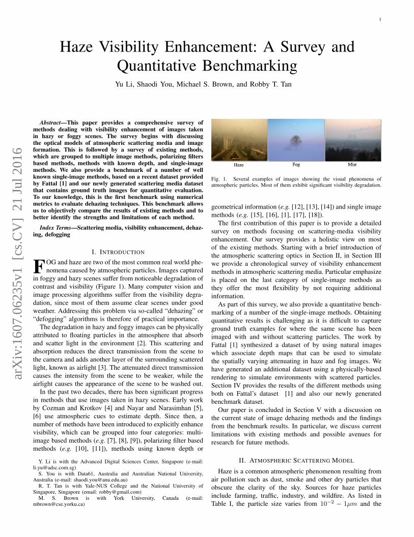
in foggy and hazy scenes suffer from noticeable degradation ofcontrast and visibility (Figure 1). Many computer vision andimage processing algorithms suffer from the visibility degra-dation, since most of them assume clear scenes under goodweather. Addressing this problem via so-called “dehazing” or“defogging” algorithms is therefore of practical importance.

The degradation in hazy and foggy images can be physicallyattributed to floating particles in the atmosphere that absorband scatter light in the environment [2]. This scattering andabsorption reduces the direct transmission from the scene tothe camera and adds another layer of the surrounding scatteredlight, known as airlight [3]. The attenuated direct transmissioncauses the intensity from the scene to be weaker, while theairlight causes the appearance of the scene to be washed out.

In the past two decades, there has been significant progressin methods that use images taken in hazy scenes. Early workby Cozman and Krotkov [4] and Nayar and Narasimhan [5],[6] use atmospheric cues to estimate depth. Since then, anumber of methods have been introduced to explicitly enhancevisibility, which can be grouped into four categories: multi-image based methods (e.g. [7], [8], [9]), polarizing filter basedmethods (e.g. [10], [11]), methods using known depth or

Y. Li is with the Advanced Digital Sciences Center, Singapore (e-mail:li.yu@adsc.com.sg)

S. You is with Data61, Australia and Australian National University,Australia (e-mail: shaodi.you@anu.edu.au)

R. T. Tan is with Yale-NUS College and the National University ofSingapore, Singapore (email: robby@gmail.com)

M. S. Brown is with York University, Canada (e-mail:mbrown@cse.yorku.ca)

Fig. 1. Several examples of images showing the visual phenomena ofatmospheric particles. Most of them exhibit significant visibility degradation.

geometrical information (e.g. [12], [13], [14]) and single imagemethods (e.g. [15], [16], [1], [17], [18]).

The first contribution of this paper is to provide a detailedsurvey on methods focusing on scattering-media visibilityenhancement. Our survey provides a holistic view on mostof the existing methods. Starting with a brief introduction ofthe atmospheric scattering optics in Section II, in Section IIIwe provide a chronological survey of visibility enhancementmethods in atmospheric scattering media. Particular emphasizeis placed on the last category of single-image methods asthey offer the most flexibility by not requiring additionalinformation.

As part of this survey, we also provide a quantitative bench-marking of a number of the single-image methods. Obtainingquantitative results is challenging as it is difficult to captureground truth examples for where the same scene has beenimaged with and without scattering particles. The work byFattal [1] synthesized a dataset of by using natural imageswhich associate depth maps that can be used to simulatethe spatially varying attenuating in haze and fog images. Wehave generated an additional dataset using a physically-basedrendering to simulate environments with scattered particles.Section IV provides the results of the different methods usingboth on Fattal’s dataset [1] and also our newly generatedbenchmark dataset.

Our paper is concluded in Section V with a discussion onthe current state of image dehazing methods and the findingsfrom the benchmark results. In particular, we discuss currentlimitations with existing methods and possible avenues forresearch for future methods.

II. ATMOSPHERIC SCATTERING MODEL

Haze is a common atmospheric phenomenon resulting fromair pollution such as dust, smoke and other dry particles thatobscure the clarity of the sky. Sources for haze particlesinclude farming, traffic, industry, and wildfire. As listed inTable I, the particle size varies from 10−2 − 1µm and the

arX

iv:1

607.

0623

5v1

[cs

.CV

] 2

1 Ju

l 201

6

2

TABLE IWEATHER CONDITION AND THE PARTICLE TYPE, SIZE AND DENSITY.

Weather Particle type Particle radius

(𝝁𝒎) Density (𝒄𝒎−𝟑)

Clean air Molecule 10−4 1019

Haze Aerosol 10−2 − 1 10 − 103

Fog Water droplets 1 − 10 10 − 100

We follow the definition of Hidy [19].

Incident light

Intensity distribution

of scattered light

(a) Single particle scattering

(b) Unite volume scattering

𝜃

Incident light

𝐸(𝜆)

Observed intensity

𝛽 𝜃, 𝜆 𝐸(𝜆)

(c) Attenuation over distance

Incident light

𝐸(0, 𝜆)Attenuated light

𝐸(𝑥, 𝜆)

𝑥 = 0 𝑥 = 𝑑d𝑥

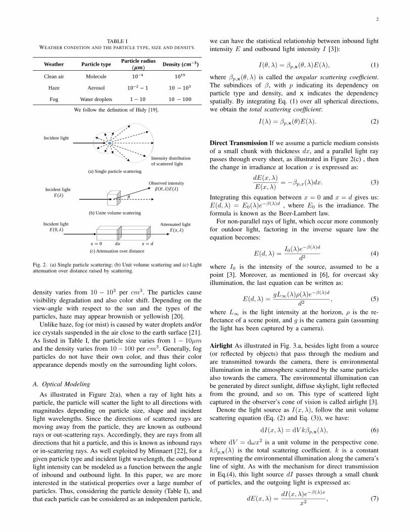
Fig. 2. (a) Single particle scattering; (b) Unit volume scattering and (c) Lightattenuation over distance raised by scattering.

density varies from 10 − 103 per cm3. The particles causevisibility degradation and also color shift. Depending on theview-angle with respect to the sun and the types of theparticles, haze may appear brownish or yellowish [20].

Unlike haze, fog (or mist) is caused by water droplets and/orice crystals suspended in the air close to the earth surface [21].As listed in Table I, the particle size varies from 1 − 10µmand the density varies from 10− 100 per cm3. Generally, fogparticles do not have their own color, and thus their colorappearance depends mostly on the surrounding light colors.

A. Optical Modeling

As illustrated in Figure 2(a), when a ray of light hits aparticle, the particle will scatter the light to all directions withmagnitudes depending on particle size, shape and incidentlight wavelengths. Since the directions of scattered rays aremoving away from the particle, they are known as outboundrays or out-scattering rays. Accordingly, they are rays from alldirections that hit a particle, and this is known as inbound raysor in-scattering rays. As well exploited by Minnaert [22], for agiven particle type and incident light wavelength, the outboundlight intensity can be modeled as a function between the angleof inbound and outbound light. In this paper, we are moreinterested in the statistical properties over a large number ofparticles. Thus, considering the particle density (Table I), andthat each particle can be considered as an independent particle,

we can have the statistical relationship between inbound lightintensity E and outbound light intensity I [3]):

I(θ, λ) = βp,x(θ, λ)E(λ), (1)

where βp,x(θ, λ) is called the angular scattering coefficient.The subindices of β, with p indicating its dependency onparticle type and density, and x indicates the dependencyspatially. By integrating Eq. (1) over all spherical directions,we obtain the total scattering coefficient:

I(λ) = βp,x(θ)E(λ). (2)

Direct Transmission If we assume a particle medium consistsof a small chunk with thickness dx, and a parallel light raypasses through every sheet, as illustrated in Figure 2(c) , thenthe change in irradiance at location x is expressed as:

dE(x, λ)

E(x, λ)= −βp,x(λ)dx. (3)

Integrating this equation between x = 0 and x = d gives us:E(d, λ) = E0(λ)e−β(λ)d , where E0 is the irradiance. Theformula is known as the Beer-Lambert law.

For non-parallel rays of light, which occur more commonlyfor outdoor light, factoring in the inverse square law theequation becomes:

E(d, λ) =I0(λ)e−β(λ)d

d2(4)

where I0 is the intensity of the source, assumed to be apoint [3]. Moreover, as mentioned in [6], for overcast skyillumination, the last equation can be written as:

E(d, λ) =gL∞(λ)ρ(λ)e−β(λ)d

d2, (5)

where L∞ is the light intensity at the horizon, ρ is the re-flectance of a scene point, and g is the camera gain (assumingthe light has been captured by a camera).

Airlight As illustrated in Fig. 3.a, besides light from a source(or reflected by objects) that pass through the medium andare transmitted towards the camera, there is environmentalillumination in the atmosphere scattered by the same particlesalso towards the camera. The environmental illumination canbe generated by direct sunlight, diffuse skylight, light reflectedfrom the ground, and so on. This type of scattered lightcaptured in the observer’s cone of vision is called airlight [3].

Denote the light source as I(x, λ), follow the unit volumescattering equation (Eq. (2) and Eq. (3)), we have:

dI(x, λ) = dV kβp,x(λ), (6)

where dV = dωx2 is a unit volume in the perspective cone.kβp,x(λ) is the total scattering coefficient. k is a constantrepresenting the environmental illumination along the camera’sline of sight. As with the mechanism for direct transmissionin Eq.(4), this light source dI passes through a small chunkof particles, and the outgoing light is expressed as:

dE(x, λ) =dI(x, λ)e−β(λ)x

x2, (7)

3

d𝜔

d𝑥

𝑑

𝑥

Air lightScene reflection

(a) Imagery model

𝑅(𝒙, 𝜆)

Captured image 𝐼(𝒙, 𝜆)

(b) Formula of illumination components

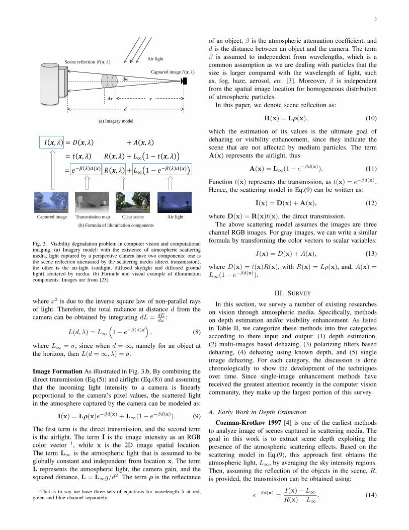
𝐼 𝒙, 𝜆 = 𝐷 𝒙, 𝜆 + 𝐴 𝒙, 𝜆

= 𝑡 𝒙, 𝜆 𝑅 𝒙, 𝜆 + 𝐿∞ 1 − 𝑡 𝒙, 𝜆

= 𝑒−𝛽 𝜆 𝑑(𝒙) 𝑅 𝒙, 𝜆 + 𝐿∞ 1 − 𝑒−𝛽 𝜆 𝑑(𝒙)

Captured image Clear sceneTransmission map Air light

Fig. 3. Visibility degradation problem in computer vision and computationalimaging. (a) Imagery model: with the existence of atmospheric scatteringmedia, light captured by a perspective camera have two components: one isthe scene reflection attenuated by the scattering media (direct transmission),the other is the air-light (sunlight, diffused skylight and diffused groundlight) scattered by media. (b) Formula and visual example of illuminationcomponents. Images are from [23].

where x2 is due to the inverse square law of non-parallel raysof light. Therefore, the total radiance at distance d from thecamera can be obtained by integrating dL = dE

dω :

L(d, λ) = L∞(

1− e−β(λ)d), (8)

where L∞ = σ, since when d = ∞, namely for an object atthe horizon, then L(d =∞, λ) = σ.

Image Formation As illustrated in Fig. 3.b, By combining thedirect transmission (Eq.(5)) and airlight (Eq.(8)) and assumingthat the incoming light intensity to a camera is linearlyproportional to the camera’s pixel values, the scattered lightin the atmosphere captured by the camera can be modeled as:

I(x) = Lρ(x)e−βd(x) + L∞(1− e−βd(x)). (9)

The first term is the direct transmission, and the second termis the airlight. The term I is the image intensity as an RGBcolor vector 1, while x is the 2D image spatial location.The term L∞ is the atmospheric light that is assumed to beglobally constant and independent from location x. The termL represents the atmospheric light, the camera gain, and thesquared distance, L = L∞g/d2. The term ρ is the reflectance

1That is to say we have three sets of equations for wavelength λ at red,green and blue channel separately.

of an object, β is the atmospheric attenuation coefficient, andd is the distance between an object and the camera. The termβ is assumed to independent from wavelengths, which is acommon assumption as we are dealing with particles that thesize is larger compared with the wavelength of light, suchas, fog, haze, aerosol, etc. [3]. Moreover, β is independentfrom the spatial image location for homogeneous distributionof atmospheric particles.

In this paper, we denote scene reflection as:

R(x) = Lρ(x), (10)

which the estimation of its values is the ultimate goal ofdehazing or visibility enhancement, since they indicate thescene that are not affected by medium particles. The termA(x) represents the airlight, thus

A(x) = L∞(1− e−βd(x)). (11)

Function t(x) represents the transmission, as t(x) = e−βd(x).Hence, the scattering model in Eq.(9) can be written as:

I(x) = D(x) + A(x), (12)

where D(x) = R(x)t(x), the direct transmission.The above scattering model assumes the images are three

channel RGB images. For gray images, we can write a similarformula by transforming the color vectors to scalar variables:

I(x) = D(x) +A(x), (13)

where D(x) = t(x)R(x), with R(x) = Lρ(x), and, A(x) =L∞(1− e−βd(x)).

III. SURVEY

In this section, we survey a number of existing researcheson vision through atmospheric media. Specifically, methodson depth estimation and/or visibility enhancement. As listedin Table II, we categorize these methods into five categoriesaccording to there input and output: (1) depth estimation,(2) multi-images based dehazing, (3) polarizing filters baseddehazing, (4) dehazing using known depth, and (5) singleimage dehazing. For each category, the discussion is donechronologically to show the development of the techniquesover time. Since single-image enhancement methods havereceived the greatest attention recently in the computer visioncommunity, they make up the largest portion of this survey.

A. Early Work in Depth Estimation

Cozman-Krotkov 1997 [4] is one of the earliest methodsto analyze image of scenes captured in scattering media. Thegoal in this work is to extract scene depth exploiting thepresence of the atmospheric scattering effects. Based on thescattering model in Eq.(9), this approach first obtains theatmospheric light, L∞, by averaging the sky intensity regions.Then, assuming the reflection of the objects in the scene, R,is provided, the transmission can be obtained using:

e−βd(x) =I(x)− L∞R(x)− L∞

. (14)

4

TABLE IIAN OVERVIEW OF EXISTING WORKS ON VISION THROUGH ATMOSPHERIC SCATTERING MEDIA.

Method Category Known Parameters (Input) Estimating (Output) Key idea

Cozman – Krotkov 1997 Depth estimationSingle grayscale image I(x)

Scene reflection R(x)

Transmission t(x);

depth d(x);Direct solving

Nayar – Narasimham 1999

Method 1Depth estimation

Two grayscale images I(x) with different

scattering coefficients 𝛽1, 𝛽2t(x), d(x) Comparing different 𝛽

Nayar – Narasimham 1999

Method 2Depth estimation

Single grayscale image I(x)

Atmospheric light 𝐿∞

t(x), d(x)Direct solving

Nayar – Narasimham 1999

Method 3Depth estimation Single RGB image I(x)

t(x), d(x) ,

Air light: A(x),Dichromatic model

Nayar – Narasimham 2000 Multi-imagesTwo RGB images I(x)

with different weather conditions 𝛽1, 𝛽2t(x), d(x) Iso – depth: Comparing different 𝛽; colour decomposition

Nayar – Narasimham 2003a Multi-imagesTwo grayscale or RGB images I(x) with

different weather conditions 𝛽1, 𝛽2

t(x), d(x), A(x) and

Scene reflection R(x)Iso – depth

Caraffa-Tarel 2012 Multi-images Stereo Cameras d(x), R(x)Depth from scattering; Depth from stereo;

Spatial smoothness

Li et al. 2015 Multi-images Monocular video t(x), d(x), R(x)Depth from monocular video;

Depth from scattering; Photoconsistency

Schechner et al. 2001 Polarizing Filter

Two images with different polarization

under same weather condition

Image with sky region presented

A(x), t(x), d(x), R(x)Assuming direct transmission D(x) has insignificant

polarization

Schartz et al. 2006 Polarizing FilterTwo images with different polarization

under same weather condition

Image with sky region presented

A(x), t(x), d(x), R(x)Direct transmission D(x) has insignificant polarization

A(x) and D (x) are statistically independent

Oakley – Satherley 1998 Known DepthSingle grayscale image I(x)

Depth d(x)

Atmospheric light: 𝑳∞Scattering coefficient: 𝛽

R(x)

Mean square optimization

Colour of the scene is uniform

Nayar – Narasimham 2003b

Method 1Known Depth

Single RGB image I(x)

User specified less hazed and more

hazed regions

R(x) Dichromatic model

Nayar – Narasimham 2003b

Method 2

Known DepthSingle RGB image I(x)

User specified vanishing point, min

depth and max depth

R(x) Dichromatic model

Hautiere et al. 2007 Known DepthSingle image I(x)

Scene of flat ground𝑳∞, R(x) Depth from calibrated camera

Kopf et al. 2008 Known DepthSingle image I(x)

Known 3D modelt(x), R(x)

Transmission estimation using averaged texture

from same depth

Tan 2008 Single image Single RGB image I(x) 𝑳∞, t(x), R(x)

Brightest value assumption for Atmospheric light 𝐿∞estimation; Maximal contrast assumption for Scene reflection

R(x) estimation

Fattal 2008Single image

Single RGB image I(x) 𝑳∞, t(x), R(x)Shading and transmission are locally and statistically

uncorrelated

He et al. 2009 Single image Single RGB image I(x) 𝑳∞, t(x), R(x)Dark channel: outdoor objects in clear weather have at least

one colour channel that is significantly dark

Tarel – Hautiere 2009 Single image Single RGB image I(x) 𝑳∞, t(x), R(x)Maximal contrast assumption;

Normalized air light is upper-bounded

Kratz – Nishino 2009 Single image Single RGB image I(x) t(x), R(x)Scene reflection R(x) and Air light A(x) are statistically

independent; Layer separation

Ancuti-Ancuti 2010 Single image Single RGB image I(x) A(x), R(x)Gray-world colour constancy;

Global contrast enhancement

Meng et al. 2013 Single image Single RGB image I(x) 𝑳∞, t (x), R(x) Dark channel for transmission t(x)

Tang et al. 2014 Single image Single RGB image I(x) t (x), R(x) Machine learning of transmission t(x)

Fattal 2014 Single image Single RGB image I(x) 𝑳∞, t (x), R(x)Colour line: small image patch has uniform colour and depth

but different shading

Cai et al. 2016 Single image Single RGB image I(x) t (x), R(x) Learning of t(x) in CNN framework

Berman et al. 2016 Single image Single RGB image I(x) t (x), R(x) Non-local haze line; finite colour approximation

5

However, the absolute depth, d(x), will still be unknown sincethe value of β is unknown. To resolve this, we need two pixelsthat have the same value of β to obtain the relative depth, suchthat:

d(xi)

d(xj)=

log(I(xi)−L∞R(xi)−L∞

)

log(I(xj)−L∞R(xj)−L∞

) , (15)

where xi 6= xj . If we have a reference point in the input imagewhose depth is known, then we can obtain the absolute depthof every pixel in the image. Note that, R is given from animage of exactly the same scene taken in a clear day, thoughof course, it is a considerably rough approximation; since evenin a clear day, an outdoor image is always affected by mediumparticles, particularly for faraway objects.

Nayar-Narasimhan 1999 [5] and later [6] propose three d-ifferent algorithms to estimate depth from hazy scenes. Unlike[4], however, this work does not assume that the reflection, R,of the scene without the effects of haze is provided. The firstof the three algorithms employs only the direct transmission toestimate the relative depths of light sources from two imagestaken under different scattering coefficients at nighttime. Theidea is to apply the logarithm to the ratio of the pixel intensitiesof the two input images (where the airlight is assumed to beignorable at nighttime). Given gray images of nighttime whereonly the light sources are visible, we compute:

K(x) =I1(x)

I2(x)=D1(x)

D2(x)= e−(β1−β2)d(x), (16)

where index 1, 2 indicates the first and second images. Theterm D is the direct transmission (Eq.(13)). The relative depthfrom two pairs of pixels can be obtained by:

logK(xi)

logK(xj)=d(xj)

d(xj). (17)

This relative depth is not for the entire image, but only for thelight source regions.

The second algorithm is to estimate the absolute depth froma single airlight image. It assumes that the atmospheric light,L∞, and achromatic airlight, A(x), are given:

log

(L∞ −A(x)

L∞

)= −βd(x). (18)

The problem with this algorithm is with regards obtaining theairlight, which is discussed in the third algorithm.

The third algorithm treats the problem of depth estimationas a color decomposition of the scattering model (Eq.(9)). Themethod decomposes the input images into the chromaticity ofthe direct attenuation and the chromaticity of the airlight; thelatter is identical to the chromaticity of the atmospheric light.Chromaticity is generally defined as a normalized color, whereR/(R + G + B), and G/(R + G + B). This is a unit colorvector and can be used to convert the model of Eq.(9) into achromaticity based formulation:

I(x) = p(x)D(x) + q(x)A(x), (19)

where D and A are the chromaticity values of the directtransmission and the airlight. The terms p and q are the mag-nitude of the direct transmission and the airlight, respectively.

The paper calls the equation the dichromatic scattering model,where the word dichromatic is borrowed from [24] due to thesimilarity of the models.

In the RGB space, the two chromaticity vectors (the directtransmission chromaticity and airlight chromaticity) will createa plane. The same idea had been discussed in [24][25] for thedichromatic model of specular highlights. Accordingly, givena pixel and the two chromaticity values, we can immediatelycalculate the magnitude of the airlight, which consequentlygives us the absolute depth map by employing Eq.(18). Inthis algorithm, the chromaticity of the direct transmission isassumed to be given from a clear day image of exactly thesame scene, and the airlight chromaticity is computed from aknown atmospheric light.

B. Multiple Images

Narasimhan-Nayar 2000 [7] extends the analysis of thedichromatic scattering model of [5] in Eq.(19) by usingmultiple images of the same scene taken in different hazedensity. The method works by supposing there are two imagestaken from the same scene, which share the same color ofatmospheric light, but different colors of direct transmission.From this, two planes can be formed in the RGB space thatintersect to each other. In their work [7] utilizes the intersec-tion to estimate the atmospheric light chromaticity, A, which issimilar to Tominaga and Wandell’s method [26] for estimatinga light color from specular reflection. The assumption thatthe images of the same scene have different colors of directtransmission, however, might produce inaccurate estimationsince, in many cases, the colors of the direct transmission ofthe same scene are similar.

The method then introduces the concept of iso-depth, whichis the ratio of the direct transmission magnitudes under two d-ifferent weather conditions. Referring to Eq.(19), and applyingit to two images, we have:

p2(x)

p1(x)=L∞2

L∞1e−(β2−β1)d(x), (20)

where p is the magnitude of the direct transmission. From thisequation, we can infer that if two pairs of pixels have the sameratio, then they must have the same depth: p2(xi)

p1(xi)=

p2(xj)p1(xj)

.To calculate these ratios, the method provides a solution byutilizing the analysis of the planes formed in the RGB spaceby the scattering dichromatic model in Eq.(19).

Having obtained the ratios for all pixels, the method pro-ceeds with the estimation of the scene structure, which iscalculated by:

(β2 − β1)d(x) = log

(L∞2

L∞1

)− log

(p2(x)

p1(x)

). (21)

To be able to estimate the depth, the last equation requires theknowledge of the values of L∞1 and L∞2, which are obtainedby solving the following linear equation:

c(x) = L∞2 −p2(x)

p1(x)L∞1, (22)

where c is the magnitude of a vector indicating the distancebetween the origin of vector I1 to the origin of vector I2 in

6

the direction of the airlight chromaticity in RGB space. While,p2(x)p1(x) is the ratio, which had been computed.

For the true scene color restoration, employing the estimatedatmospheric light, the method computes the airlight magnitudeof Eq.(19) using:

q(xi) = L∞(

1− e−βd(xi)), (23)

where:

βd(xi) = βd(xj)

(d(xi)

d(xj)

), (24)

and d(xi)d(xj)

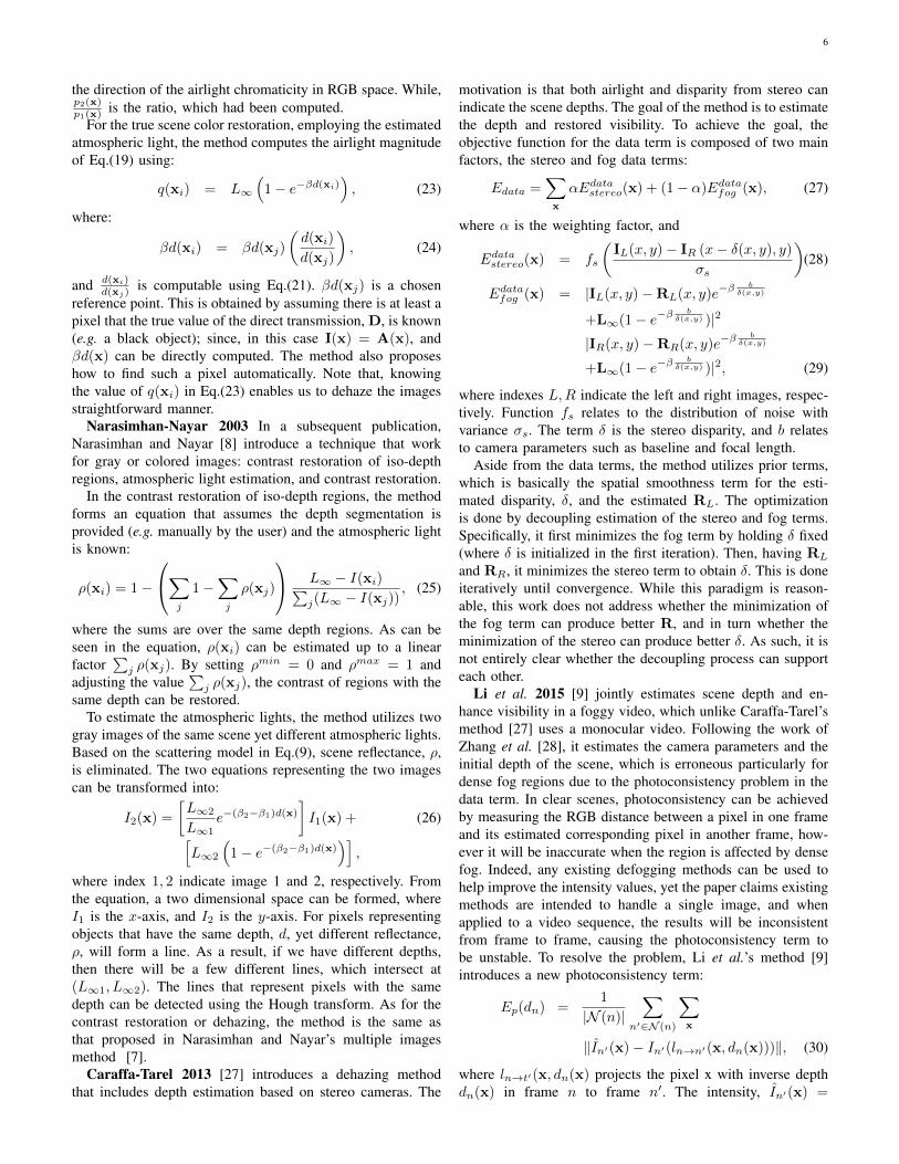
is computable using Eq.(21). βd(xj) is a chosenreference point. This is obtained by assuming there is at least apixel that the true value of the direct transmission, D, is known(e.g. a black object); since, in this case I(x) = A(x), andβd(x) can be directly computed. The method also proposeshow to find such a pixel automatically. Note that, knowingthe value of q(xi) in Eq.(23) enables us to dehaze the imagesstraightforward manner.

Narasimhan-Nayar 2003 In a subsequent publication,Narasimhan and Nayar [8] introduce a technique that workfor gray or colored images: contrast restoration of iso-depthregions, atmospheric light estimation, and contrast restoration.

In the contrast restoration of iso-depth regions, the methodforms an equation that assumes the depth segmentation isprovided (e.g. manually by the user) and the atmospheric lightis known:

ρ(xi) = 1−

∑

j

1−∑

j

ρ(xj)

L∞ − I(xi)∑

j(L∞ − I(xj)), (25)

where the sums are over the same depth regions. As can beseen in the equation, ρ(xi) can be estimated up to a linearfactor

∑j ρ(xj). By setting ρmin = 0 and ρmax = 1 and

adjusting the value∑j ρ(xj), the contrast of regions with the

same depth can be restored.To estimate the atmospheric lights, the method utilizes two

gray images of the same scene yet different atmospheric lights.Based on the scattering model in Eq.(9), scene reflectance, ρ,is eliminated. The two equations representing the two imagescan be transformed into:

I2(x) =

[L∞2

L∞1e−(β2−β1)d(x)

]I1(x) + (26)

[L∞2

(1− e−(β2−β1)d(x)

)],

where index 1, 2 indicate image 1 and 2, respectively. Fromthe equation, a two dimensional space can be formed, whereI1 is the x-axis, and I2 is the y-axis. For pixels representingobjects that have the same depth, d, yet different reflectance,ρ, will form a line. As a result, if we have different depths,then there will be a few different lines, which intersect at(L∞1, L∞2). The lines that represent pixels with the samedepth can be detected using the Hough transform. As for thecontrast restoration or dehazing, the method is the same asthat proposed in Narasimhan and Nayar’s multiple imagesmethod [7].

Caraffa-Tarel 2013 [27] introduces a dehazing methodthat includes depth estimation based on stereo cameras. The

motivation is that both airlight and disparity from stereo canindicate the scene depths. The goal of the method is to estimatethe depth and restored visibility. To achieve the goal, theobjective function for the data term is composed of two mainfactors, the stereo and fog data terms:

Edata =∑

x

αEdatastereo(x) + (1− α)Edatafog (x), (27)

where α is the weighting factor, and

Edatastereo(x) = fs

(IL(x, y)− IR (x− δ(x, y), y)

σs

)(28)

Edatafog (x) = |IL(x, y)−RL(x, y)e−βb

δ(x,y)

+L∞(1− e−β bδ(x,y) )|2

|IR(x, y)−RR(x, y)e−βb

δ(x,y)

+L∞(1− e−β bδ(x,y) )|2, (29)

where indexes L,R indicate the left and right images, respec-tively. Function fs relates to the distribution of noise withvariance σs. The term δ is the stereo disparity, and b relatesto camera parameters such as baseline and focal length.

Aside from the data terms, the method utilizes prior terms,which is basically the spatial smoothness term for the esti-mated disparity, δ, and the estimated RL. The optimizationis done by decoupling estimation of the stereo and fog terms.Specifically, it first minimizes the fog term by holding δ fixed(where δ is initialized in the first iteration). Then, having RL

and RR, it minimizes the stereo term to obtain δ. This is doneiteratively until convergence. While this paradigm is reason-able, this work does not address whether the minimization ofthe fog term can produce better R, and in turn whether theminimization of the stereo can produce better δ. As such, it isnot entirely clear whether the decoupling process can supporteach other.

Li et al. 2015 [9] jointly estimates scene depth and en-hance visibility in a foggy video, which unlike Caraffa-Tarel’smethod [27] uses a monocular video. Following the work ofZhang et al. [28], it estimates the camera parameters and theinitial depth of the scene, which is erroneous particularly fordense fog regions due to the photoconsistency problem in thedata term. In clear scenes, photoconsistency can be achievedby measuring the RGB distance between a pixel in one frameand its estimated corresponding pixel in another frame, how-ever it will be inaccurate when the region is affected by densefog. Indeed, any existing defogging methods can be used tohelp improve the intensity values, yet the paper claims existingmethods are intended to handle a single image, and whenapplied to a video sequence, the results will be inconsistentfrom frame to frame, causing the photoconsistency term tobe unstable. To resolve the problem, Li et al.’s method [9]introduces a new photoconsistency term:

Ep(dn) =1

|N (n)|∑

n′∈N (n)

∑

x

‖In′(x)− In′(ln→n′(x, dn(x)))‖, (30)

where ln→t′(x, dn(x) projects the pixel x with inverse depthdn(x) in frame n to frame n′. The intensity, In′(x) =

7

(In(x)−L∞)πn→n′ (x,tn(x))tn(x) +L∞, is a synthetic intensity val-

ue obtained from the transmission, tn, which is computable byknowing dn (note that, in the paper, the scattering coefficientβ and the atmospheric light, L∞, are estimated separately).The projection function πn→n′(x, tn(x)) computes the corre-sponding transmission in the n′-th frame for the pixel x in then-th frame with transmission tn(x). The denominator N (t)represents the neighboring frames of frame n and |N (n)| isthe number of neighboring frames. By having β(x) estimatedseparately, tn(x) depends only on dn(x), and thus dn is theonly unknown in the last equation. The whole idea in thephotoconsistency term here is to generate a synthetic intensityvalue of each pixel from known depth, d , atmosphericlight, L∞, and the particle scattering coefficient, β. Notethat, the paper assumes β and L∞ are uniform across thevideo sequence. Therefore, if those three values are correctlyestimated, the generated synthetic intensity values must becorrect.

Aside from the photoconsistency term, the method also usesLaplacian smoothing as the transmission smoothness prior.The whole framework is an integrated framework, where aftera few iterations, the outcomes are estimated depth maps anddefogged images.

C. Polarizing Filter

Schechner et al. 2001 addresses the issue appeared inthe work of Narasimhan and Nayar [7], where it requiresat least two images of the same scene taken under differentparticle densities (i.e. we have to wait until the fog densitychanges considerably). Unlike [7], Schecher et al.’s [10] usesmultiple images captured using polarizing filters, which doesnot require the fog density to change.

The main assumption employed in this polarized-basedmethod is that the direct transmission has insignificant polar-ization, and thus the polarization of the airlight dominates theobserved light. Based on this, the maximum intensity occurswhen airlight passes the through the filter. This can be obtainedwhen:

Imax(x) = D(x)/2 +Amax(x), (31)

where D and A are the direct transmission and the airlight,respectively. The minimum intensity (i.e. when the filter canblock the airlight at its best) is when:

Imin(x) = D(x)/2 +Amin(x). (32)

Adding up the two states of the polarization, we obtain:I(x) = Imax(x) + Imin(x). Based on this, the method esti-mates the atmospheric light from a sky region and computesits degree of polarization:

P =Lmax∞ − Lmin

∞Lmin∞ + Lmax∞

, (33)

and then, estimate the airlight for every pixel:

A(x) =Imax(x)− Imin(x)

P. (34)

Based on the airlight, the method computes the transmission:e−βd(x) = 1 − A(x)

L∞, and finally obtains the dehazing result

R(x) = [I(x)−A(x)] eβd(x). To obtain the maximum andthe minimum intensity values, the filter needs to be rotatedeither automatically or manually.

Shwartz et al. 2006 [11] uses the same setup proposed bySchechner et al.’s [10] but removes the assumption that skyregions are present in the input image. Instead, this methodestimates the color of the airlight and of the direct transmissionby applying independent component analysis (ICA):

[AD

]= W

[Imax

Imin

](35)

W =

[1/P −1/P

(P − 1)/P (P + 1)/P

]. (36)

In this case, the challenge lies in estimating W given[Imax, Imin]T to produce D and A accurately.

The method claims that while the airlight and direct trans-mission are in fact statistically not independent and certaintransformations such as a wavelet transformation can relax thedependence. The method therefore transforms the input datausing a wavelet transformation, solves the ICA problem byusing an optimization method in the wavelet domain. Asidefrom P , the method also needs to estimate L∞, which is doneby labeling certain regions manually to have two pixels thathave the same values of the direct transmission yet differentvalues of the airlight.

D. Known Depth

Oakley-Satherley 1998 [12] is one of the early methodsdealing with visibility enhancement in a single foggy image.The enhancement is done in two stages: parameter estimationfollowed by contrast enhancement. The basic idea of theparameter estimation is to employ the sum of squares methodto minimize an error function, between the image intensityand some parameters of the physical model, by assuming thereflectance of the scene can be approximated by a single valuerepresenting the mean of the scene reflectance. With theseassumptions, the minimization is done to estimate three globalparameters: the atmospheric light (L∞), the mean reflectanceof the whole scene ρ, and the scattering coefficient, β:

Err =M∑

x

(I(x)− L∞

(1 + (ρ− 1)e−βd(x)

))2

. (37)

The last equation assumes that L = L∞. Having estimatedthe three global parameters by minimizing function Err, theairlight is then computed using:

A(x) = L∞(1− e−βd(x)). (38)

Consequently, the end result is obtained by computing:

R(x) =

(Lmax

(I(x)−A(x)

L∞eβd(x)

)) 12.2

, (39)

where Lmax is a constant depending on the maximum graylevel of the image display device, and 1

2.2 is to compensatethe gamma correction.

8

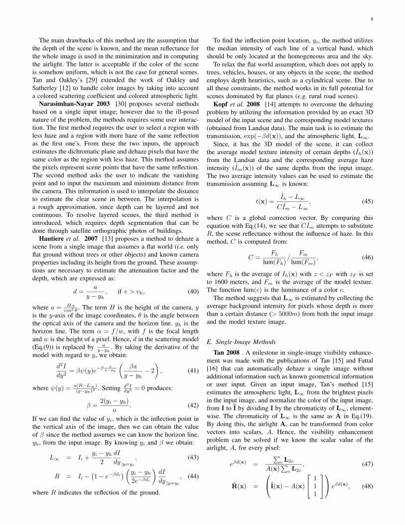
The main drawbacks of this method are the assumption thatthe depth of the scene is known, and the mean reflectance forthe whole image is used in the minimization and in computingthe airlight. The latter is acceptable if the color of the sceneis somehow uniform, which is not the case for general scenes.Tan and Oakley’s [29] extended the work of Oakley andSatherley [12] to handle color images by taking into accounta colored scattering coefficient and colored atmospheric light.

Narasimhan-Nayar 2003 [30] proposes several methodsbased on a single input image; however due to the ill-posednature of the problem, the methods requires some user interac-tion. The first method requires the user to select a region withless haze and a region with more haze of the same reflectionas the first one’s. From these the two inputs, the approachestimates the dichromatic plane and dehaze pixels that have thesame color as the region with less haze. This method assumesthe pixels represent scene points that have the same reflection.The second method asks the user to indicate the vanishingpoint and to input the maximum and minimum distance fromthe camera. This information is used to interpolate the distanceto estimate the clear scene in between. The interpolation isa rough approximation, since depth can be layered and notcontinuous. To resolve layered scenes, the third method isintroduced, which requires depth segmentation that can bedone through satellite orthographic photos of buildings.

Hautiere et al. 2007 [13] proposes a method to dehaze ascene from a single image that assumes a flat world (i.e. onlyflat ground without trees or other objects) and known cameraproperties including its height from the ground. These assump-tions are necessary to estimate the attenuation factor and thedepth, which are expressed as:

d =a

y − yh, if v > vh, (40)

where a = Hαcos2 θ . The term H is the height of the camera, y

is the y-axis of the image coordinates, θ is the angle betweenthe optical axis of the camera and the horizon line. yh is thehorizon line. The term α = f/w, with f is the focal lengthand w is the height of a pixel. Hence, d in the scattering model(Eq.(9)) is replaced by a

y−yh . By taking the derivative of themodel with regard to y, we obtain:

d2I

dy2= βψ(y)e

−β ay−yh

(βa

y − yh− 2

), (41)

where ψ(y) = a(R−L∞)(y−yh)3 . Setting d2I

dy2 = 0 produces:

β =2(yi − yh)

a. (42)

If we can find the value of yi, which is the inflection point inthe vertical axis of the image, then we can obtain the valueof β since the method assumes we can know the horizon line,yh, from the input image. By knowing yi and β we obtain:

L∞ = Ii +yi − yh

2

dI

dy |y=yi

, (43)

R = Ii −(1− e−βdi

)(yi − yh2e−βdi

)dI

dy |y=yi

, (44)

where R indicates the reflection of the ground.

To find the inflection point location, yi, the method utilizesthe median intensity of each line of a vertical band, whichshould be only located at the homogeneous area and the sky.

To relax the flat world assumption, which does not apply totrees, vehicles, houses, or any objects in the scene, the methodemploys depth heuristics, such as a cylindrical scene. Due toall these constraints, the method works in its full potential forscenes dominated by flat planes (e.g. rural road scenes).

Kopf et al. 2008 [14] attempts to overcome the dehazingproblem by utilizing the information provided by an exact 3Dmodel of the input scene and the corresponding model textures(obtained from Landsat data). The main task is to estimate thetransmission, exp(−βd(x)), and the atmospheric light, L∞.

Since, it has the 3D model of the scene, it can collectthe average model texture intensity of certain depths (Ih(x))from the Landsat data and the corresponding average hazeintensity (Im(x)) of the same depths from the input image.The two average intensity values can be used to estimate thetransmission assuming L∞ is known:

t(x) =Ih − L∞CIm − L∞

, (45)

where C is a global correction vector. By comparing thisequation with Eq.(14), we see that CIm attempts to substituteR, the scene reflectance without the influence of haze. In thismethod, C is computed from:

C =Fh

lum(Fh)/

Fmlum(Fm)

, (46)

where Fh is the average of Ih(x) with z < zF with zF is setto 1600 meters, and Fm is the average of the model texture.The function lum(c) is the luminance of a color c.

The method suggests that L∞ is estimated by collecting theaverage background intensity for pixels whose depth is morethan a certain distance (> 5000m) from both the input imageand the model texture image.

E. Single-Image Methods

Tan 2008 . A milestone in single-image visibility enhance-ment was made with the publications of Tan [15] and Fattal[16] that can automatically dehaze a single image withoutadditional information such as known geometrical informationor user input. Given an input image, Tan’s method [15]estimates the atmospheric light, L∞ from the brightest pixelsin the input image, and normalize the color of the input image,from I to I by dividing I by the chromaticity of L∞, element-wise. The chromaticity of L∞ is the same as A in Eq.(19).By doing this, the airlight A, can be transformed from colorvectors into scalars, A. Hence, the visibility enhancementproblem can be solved if we know the scalar value of theairlight, A, for every pixel:

eβd(x) =

∑c L2c

A(x)∑c L2c

, (47)

R(x) =

I(x)−A(x)

111

eβd(x), (48)

9

where c represents the index of RGB channels, and R is thelight normalized color of the scene reflection, R. The valuesof A range from 0 to

∑c L2c. The key idea of the method is

to find a value of A(x) from that range that maximizes thelocal contrast of R(x). The local contrast is defined as:

Contrast(R(x)) =S∑

x,c

|∇Rc(x)|, (49)

where S is a local window whose size is empirically set to5 × 5. It was found that the correlation between the airlightand the contrast is convex.

The problem can be casted into a Markov Random Field(MRF) framework and optimized using graphcuts to estimatethe values of the airlight across the input image. The methodworks for both color and gray images and was shown ableto handle relatively thick fog. One of the drawbacks of themethod is the appearance of halos around depth discontinuitydue to the local-window based operation. Another drawback isthat when the input regions have no textures, the quantity oflocal contrast will be constant even when the airlight valuechanges. Prior to the 2008 publication, Tan et al.[31] hadintroduced a fast single dehazing method that uses a colorconstancy method [32] to estimate the color of the atmosphericlight, and utilizes the Y channel of the Y IQ color space asan approximation to do the dehazing.

Fattal 2008 [16] is based on the idea that the shading andtransmission functions are locally and statistically uncorrelat-ed. From this, the work derives the shading and transmissionfunctions from Eq.(9):

l−1(x) =1− IA(x)/||L∞||

+η

||L∞||, (50)

t(x) = 1− IA(x)− ηIR′(x)

||L∞||, (51)

where l(x) is the shading function and t(x) is the transmissionfunction. The definitions of IA and IR′ is as follows:

IA(x) =〈I(x),L∞〉||L∞||

, (52)

IR′(x) =√||Ix||2 − I2

A(x). (53)

Assuming L∞ can be obtained from the sky regions, ηis estimated by assuming the shading and the transmissionfunctions are statistically uncorrelated over a certain regionΩ. This implies that CΩ(l−1, t) = 0, where function CΩ isthe sample covariance. Hence, η can be defined based onCΩ(l−1, t) = 0:

η(x) =CΩ (IA(x), h(x))

CΩ (IR′(x), h(x)), (54)

where h(x) = (||L∞||− IA(x))/IR′(x). Obtaining the valuesof t(x) and L∞ will eventually solve the estimation of thescene reflection, R(x).

The success of the method relies on whether the statisticaldecomposition of shading and transmission can be optimum,and whether they are truly independent. Moreover, while itworks for haze, the approach was not tried on foggy scenes.

He et al. 2009. The work in [17], [33] observed an interest-ing phenomenon of outdoor natural scenes with clear visibility.They found that most outdoor objects in clear weather have atleast one color channel that is significantly dark. They arguethat this is because natural outdoor images are colorful (i.e. thebrightness varies significantly in different color channels) andfull of shadows. Hence, they define a dark channel as:

Rdark = miny∈Ω(x)

(min

c∈R,G,BRc(y)

). (55)

Because of the observation that, Rdark → 0, He etal. citehe2009 refer to this as the dark channel prior.

The dark channel prior is used to estimate the transmissionas follows. Based on Eq.(9), we can express:

Ic(x)

Lc∞= t(x)

Rc(x)

Lc∞+ 1− t(x). (56)

Assuming that we work on a local patch, Ω(x) and t(x) areconstant within the patch, t(x), then we can be written as:

miny∈Ω(x)

(minc

Ic(x)

Lc∞

)= t(x) min

y∈Ω(x)

(minc

Rc(x)

Lc∞

)

+1− t(x), (57)

and consequently, due to the dark channel prior:

t(x) = 1− miny∈Ω(x)

(minc

Ic(x)

Lc∞

), (58)

where L∞ is obtained by picking the top 0.1 % brightestpixels in the dark channel. Finally, to have a smooth and robustestimation of t(x) that can avoid the halo effects due to theuse of patches, the method employs the closed-form solutionof matting [34].

Tarel-Hautiere 2009 . One of the drawbacks of the previousmethods [15] [16] [17] [33] is the computation time. Themethods cannot be applied for real time applications, wherethe depths of the input scenes change from frame to frame.Tarel and Hautiere [35] introduce a fast visibility restorationmethod whose complexity is linear to the number of imagepixels. Inspired by the contrast enhancement [15], they ob-served that the value of the normalized airlight, A(x) (wherethe illumination color is now pure white), is always less thanW (x), where W (x) = minc(I

c(x)). Note that, Ic is the pixelintensity value of color channel c after the light normalization.Since it takes time to find the optimum value of A(x), the ideaof estimating A(x) rapidly is based on a heuristic method:

M(x) = medianΩ(x)(W )(x), (59)S(x) = M(x)−medianΩ(x)(|W −M |)(x), (60)A(x) = max (min(pS(x),W (x), 0) , (61)

where Ω(x) is a patch centered at x, and p is a constant value,chosen empirically. The last equation means 0 ≤ A(x) ≤W (x). The method utilizes a bilateral filter or median filter tohelp produce a smooth estimation of the airlight A(x).

Kratz-Nishino 2009 [36] and later [37] offer a new perspec-tive on the dehazing problem. This work poses the problemin the framework of a factorial MRF [38], which consists ofa single observation field (the input hazy image), and two

10

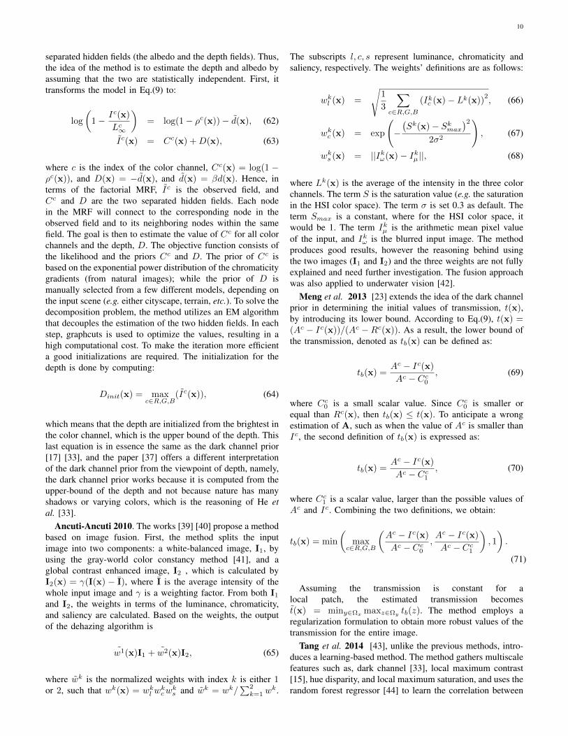
separated hidden fields (the albedo and the depth fields). Thus,the idea of the method is to estimate the depth and albedo byassuming that the two are statistically independent. First, ittransforms the model in Eq.(9) to:

log

(1− Ic(x)

Lc∞

)= log(1− ρc(x))− d(x), (62)

Ic(x) = Cc(x) +D(x), (63)

where c is the index of the color channel, Cc(x) = log(1 −ρc(x)), and D(x) = −d(x), and d(x) = βd(x). Hence, interms of the factorial MRF, Ic is the observed field, andCc and D are the two separated hidden fields. Each nodein the MRF will connect to the corresponding node in theobserved field and to its neighboring nodes within the samefield. The goal is then to estimate the value of Cc for all colorchannels and the depth, D. The objective function consists ofthe likelihood and the priors Cc and D. The prior of Cc isbased on the exponential power distribution of the chromaticitygradients (from natural images); while the prior of D ismanually selected from a few different models, depending onthe input scene (e.g. either cityscape, terrain, etc.). To solve thedecomposition problem, the method utilizes an EM algorithmthat decouples the estimation of the two hidden fields. In eachstep, graphcuts is used to optimize the values, resulting in ahigh computational cost. To make the iteration more efficienta good initializations are required. The initialization for thedepth is done by computing:

Dinit(x) = maxc∈R,G,B

(Ic(x)), (64)

which means that the depth are initialized from the brightest inthe color channel, which is the upper bound of the depth. Thislast equation is in essence the same as the dark channel prior[17] [33], and the paper [37] offers a different interpretationof the dark channel prior from the viewpoint of depth, namely,the dark channel prior works because it is computed from theupper-bound of the depth and not because nature has manyshadows or varying colors, which is the reasoning of He etal. [33].

Ancuti-Ancuti 2010. The works [39] [40] propose a methodbased on image fusion. First, the method splits the inputimage into two components: a white-balanced image, I1, byusing the gray-world color constancy method [41], and aglobal contrast enhanced image, I2 , which is calculated byI2(x) = γ(I(x) − I), where I is the average intensity of thewhole input image and γ is a weighting factor. From both I1

and I2, the weights in terms of the luminance, chromaticity,and saliency are calculated. Based on the weights, the outputof the dehazing algorithm is

w1(x)I1 + w2(x)I2, (65)

where wk is the normalized weights with index k is either 1or 2, such that wk(x) = wkl w

kcw

ks and wk = wk/

∑2k=1 w

k.

The subscripts l, c, s represent luminance, chromaticity andsaliency, respectively. The weights’ definitions are as follows:

wkl (x) =

√1

3

∑

c∈R,G,B(Ikc (x)− Lk(x))

2, (66)

wkc (x) = exp

(−(Sk(x)− Skmax

)2

2σ2

), (67)

wks (x) = ||Ikω(x)− Ikµ ||, (68)

where Lk(x) is the average of the intensity in the three colorchannels. The term S is the saturation value (e.g. the saturationin the HSI color space). The term σ is set 0.3 as default. Theterm Smax is a constant, where for the HSI color space, itwould be 1. The term Ikµ is the arithmetic mean pixel valueof the input, and Ikω is the blurred input image. The methodproduces good results, however the reasoning behind usingthe two images (I1 and I2) and the three weights are not fullyexplained and need further investigation. The fusion approachwas also applied to underwater vision [42].

Meng et al. 2013 [23] extends the idea of the dark channelprior in determining the initial values of transmission, t(x),by introducing its lower bound. According to Eq.(9), t(x) =(Ac − Ic(x))/(Ac −Rc(x)). As a result, the lower bound ofthe transmission, denoted as tb(x) can be defined as:

tb(x) =Ac − Ic(x)

Ac − Cc0, (69)

where Cc0 is a small scalar value. Since Cc0 is smaller orequal than Rc(x), then tb(x) ≤ t(x). To anticipate a wrongestimation of A, such as when the value of Ac is smaller thanIc, the second definition of tb(x) is expressed as:

tb(x) =Ac − Ic(x)

Ac − Cc1, (70)

where Cc1 is a scalar value, larger than the possible values ofAc and Ic. Combining the two definitions, we obtain:

tb(x) = min

(max

c∈R,G,B

(Ac − Ic(x)

Ac − Cc0,Ac − Ic(x)

Ac − Cc1

), 1

).

(71)

Assuming the transmission is constant for alocal patch, the estimated transmission becomest(x) = miny∈Ωx maxz∈Ωy tb(z). The method employs aregularization formulation to obtain more robust values of thetransmission for the entire image.

Tang et al. 2014 [43], unlike the previous methods, intro-duces a learning-based method. The method gathers multiscalefeatures such as, dark channel [33], local maximum contrast[15], hue disparity, and local maximum saturation, and uses therandom forest regressor [44] to learn the correlation between

11

the features and the transmission, t(x). The features related tothe transmission are defined as follows:

FD(x) = miny∈Ω(x)

minc∈R,G,B

Ic(y)

Ac,

FC(x) = maxy∈Ω(x)

√√√√ 1

3|Ω(y)|∑

z∈Ω(y)

||I(y)− I(z)||2,

FH(x) = |H(Isi(x))−H(I(x))|,

FS(x) = maxy∈Ω(x)

(1− minc I

c(y)

maxc Ic(y)

), (72)

where Isi = max[Ic(x), 1− Ic(x)]. For the learning process,synthetic patches are generated from given haze-free patches,fixed white atmospheric light, and random transmission values,where the haze-free images are taken from the Internet. Thepaper claims that the most significant feature is the darkchannel feature, however, other features also play importantroles, particularly when the color of an object is the same thatof the atmospheric light.

Fattal 2014 [1] introduces another approach based oncolor lines. This method assumes that small image patches(e.g. 7×7) have a uniformly colored surface and the samedepth, yet different shading. Hence, the model in Eq.(9) canbe written as:

I(x) = l(x)R + (1− t)L∞, (73)

where l(x) is the shading, and R(x) = l(x)R. Since theequation is a linear equation, in the RGB space the pixels ofa patch will form a straight line (unless when the assumptionsare violated, e.g. when patches containing color or depthboundaries). This line will intersect with another line formedby (1 − t)L∞. Since L∞ is assumed to be known, then byhaving the intersection, (1−t) can be obtained. To obtain t(x)for the entire image, the method has to scan the pixels, extractpatches, and find the intersections. Some patches might notgive correct intersections, however if the majority of patchesdo, then the estimation can be correct. Patches containingobject color identical to the atmospheric light color will notgive any intersection, as the lines will be parallel. A GaussianMarkov random field (GMRF) is used to do the interpolation.

Sulami et al.’s method [45] uses the same idea and as-sumptions of the local color lines to estimate the atmosphericlight, L∞, automatically. First, it estimates the color of theatmospheric light by using a few patches, minimal two patchesof different scene reflections. It assumes the two patchesprovide two different straight lines in the RGB space, andthe atmospheric light’s vector which starts from the originmust intersects with the two straight lines. Second, knowingthe normalized color vector, it tries to estimate the magnitudeof the atmospheric light. The idea is to dehaze the imageusing the estimated normalized light vector, then to minimizethe distance between the estimated shading and the estimatedtransmission for the top 1 % brightness value found at eachtransmission level.

Cai et al. 2016 [46] proposes a learning based frameworksimilar to [43] that trains a regressor to predict the transmissionvalue t(x) at each pixel (16× 16) from its surrounding patch.

TABLE IIISINGLE IMAGE DEHAZING METHODS WE COMPARED. PROGRAMMING

LANGUAGE-M:MATLAB,P:PYTHON,C:C/C++. THE AVERAGE RUNTIME ISTESTED ON IMAGES OF RESOLUTION 720× 480 USING A DESKTOP WITHXEON E5 3.5GHZ CPU AND 16GB RAM. WE USE THE CODE FROM THE

AUTHORS, EXCEPT THOSE WITH MARKER *:WE IMPLEMENTED THEMETHODS BY OURSELVES, †: WE DIRECTLY USE THE RESULTS FROM THE

AUTHOR.

Methods Pub. venue Code Runtime(s)Tarel 09 [35] ICCV 2009 M 12.8

Ancuti 13 [40] TIP 2013 M* 3.0Tan 08 [15] CVPR 2008 C 3.3

Fattal 08 [16] ToG 2008 M† 141.1He 09 [17] CVPR 2009 M* 20

Kratz 09 [36] ICCV 2009 P 124.2Meng 13 [23] ICCV 2013 M 1.0Fattal 14 [1] ToG 2014 C† 1.9

Berman 16 [18] CVPR 2016 M 1.8Tang 14 [43] CVPR 2014 M* 10.4Cai 16 [46] arXiv 2016 M* 1.7

Unlike [43] that used hand crafted feature, Cai et al. [46] ap-plied a convolutional neural network (CNN) based architecturewith special network design (See [46] for the architecture). Thenetwork, termed DehazeNet, are conceptually formed by foursequential operations (feature extraction, multi-scale mapping,local extremum and non-linear regression), that consists of3 convolution layers, a max-pooling, a Maxout unit and aBilateral Rectified Linear Unit (BReLU, a nonlinear activationfunction extended from standard ReLU [47]). The training setused is similar to that in [43], namely they gathered hazefree patches from Internet to generate hazy patches usingthe hazy imaging model with random transmissions t andassuming white atmosphere light color (L∞ = [1 1 1]>). Onceall the weights in the network are obtained from the training,the transmission estimation for a new hazy image patch issimply forward propagation using the network. To handle theblock artifact caused by the patch based estimation, guidedfiltering [48] is used to refine the transmission map.

Berman et al. 2016 [18] proposes an algorithm basedon a new, non-local prior. This is a departure from existingmethods (e.g. [15], [17], [23], [1], [43], [46] etc.) that use patchbased transmission estimation. The algorithm by [18] relieson the assumption that colors of a haze-free image are wellapproximated by a few hundred distinct colors, that form tightclusters in RGB space and pixels in a cluster are often non-local (spread in the whole images). The presence of haze willelongate the shape of each cluster to a line in color space as thepixels may be affected by different transmission coefficientsdue to their different distances to the camera. The lines, termedhaze-line, is informative in estimating the transmission factors.In their algorithm, they first proposed a clustering method togroup the pixels and each cluster becomes a haze-line. Thenthe maximum radius of each cluster is calculated and used toestimate the transmission. A final regulation step is performedto enforce the smoothness of the transmission map.

IV. QUANTITATIVE BENCHMARKING

In this section, we benchmark some visibility enhancementmethods. Our focus is on recent single-image based meth-ods. Compared with other approaches, single-image based

12

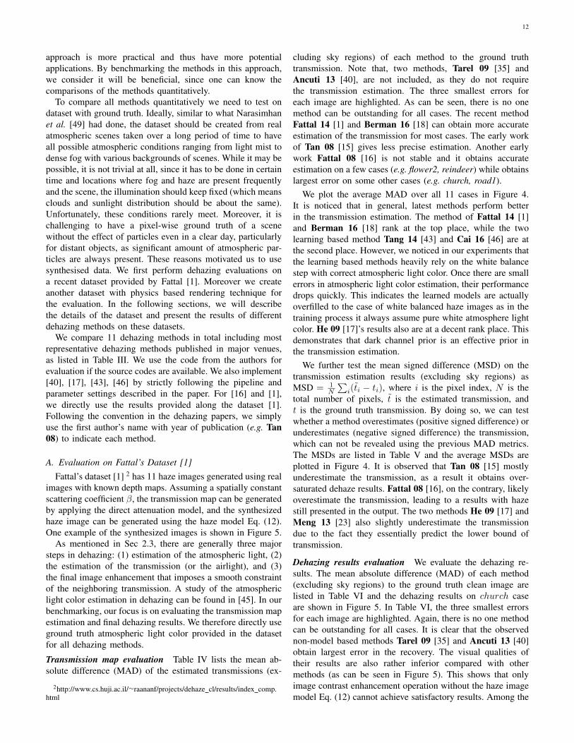
approach is more practical and thus have more potentialapplications. By benchmarking the methods in this approach,we consider it will be beneficial, since one can know thecomparisons of the methods quantitatively.

To compare all methods quantitatively we need to test ondataset with ground truth. Ideally, similar to what Narasimhanet al. [49] had done, the dataset should be created from realatmospheric scenes taken over a long period of time to haveall possible atmospheric conditions ranging from light mist todense fog with various backgrounds of scenes. While it may bepossible, it is not trivial at all, since it has to be done in certaintime and locations where fog and haze are present frequentlyand the scene, the illumination should keep fixed (which meansclouds and sunlight distribution should be about the same).Unfortunately, these conditions rarely meet. Moreover, it ischallenging to have a pixel-wise ground truth of a scenewithout the effect of particles even in a clear day, particularlyfor distant objects, as significant amount of atmospheric par-ticles are always present. These reasons motivated us to usesynthesised data. We first perform dehazing evaluations ona recent dataset provided by Fattal [1]. Moreover we createanother dataset with physics based rendering technique forthe evaluation. In the following sections, we will describethe details of the dataset and present the results of differentdehazing methods on these datasets.

We compare 11 dehazing methods in total including mostrepresentative dehazing methods published in major venues,as listed in Table III. We use the code from the authors forevaluation if the source codes are available. We also implement[40], [17], [43], [46] by strictly following the pipeline andparameter settings described in the paper. For [16] and [1],we directly use the results provided along the dataset [1].Following the convention in the dehazing papers, we simplyuse the first author’s name with year of publication (e.g. Tan08) to indicate each method.

A. Evaluation on Fattal’s Dataset [1]

Fattal’s dataset [1] 2 has 11 haze images generated using realimages with known depth maps. Assuming a spatially constantscattering coefficient β, the transmission map can be generatedby applying the direct attenuation model, and the synthesizedhaze image can be generated using the haze model Eq. (12).One example of the synthesized images is shown in Figure 5.

As mentioned in Sec 2.3, there are generally three majorsteps in dehazing: (1) estimation of the atmospheric light, (2)the estimation of the transmission (or the airlight), and (3)the final image enhancement that imposes a smooth constraintof the neighboring transmission. A study of the atmosphericlight color estimation in dehazing can be found in [45]. In ourbenchmarking, our focus is on evaluating the transmission mapestimation and final dehazing results. We therefore directly useground truth atmospheric light color provided in the datasetfor all dehazing methods.

Transmission map evaluation Table IV lists the mean ab-solute difference (MAD) of the estimated transmissions (ex-

2http://www.cs.huji.ac.il/∼raananf/projects/dehaze cl/results/index comp.html

cluding sky regions) of each method to the ground truthtransmission. Note that, two methods, Tarel 09 [35] andAncuti 13 [40], are not included, as they do not requirethe transmission estimation. The three smallest errors foreach image are highlighted. As can be seen, there is no onemethod can be outstanding for all cases. The recent methodFattal 14 [1] and Berman 16 [18] can obtain more accurateestimation of the transmission for most cases. The early workof Tan 08 [15] gives less precise estimation. Another earlywork Fattal 08 [16] is not stable and it obtains accurateestimation on a few cases (e.g. flower2, reindeer) while obtainslargest error on some other cases (e.g. church, road1).

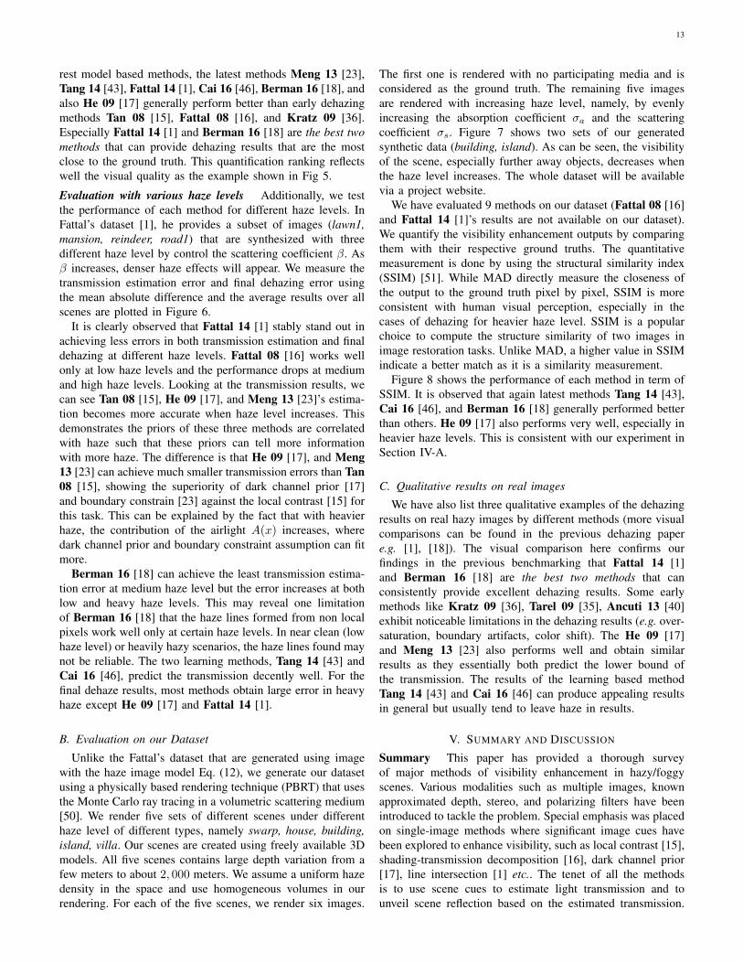
We plot the average MAD over all 11 cases in Figure 4.It is noticed that in general, latest methods perform betterin the transmission estimation. The method of Fattal 14 [1]and Berman 16 [18] rank at the top place, while the twolearning based method Tang 14 [43] and Cai 16 [46] are atthe second place. However, we noticed in our experiments thatthe learning based methods heavily rely on the white balancestep with correct atmospheric light color. Once there are smallerrors in atmospheric light color estimation, their performancedrops quickly. This indicates the learned models are actuallyoverfilled to the case of white balanced haze images as in thetraining process it always assume pure white atmosphere lightcolor. He 09 [17]’s results also are at a decent rank place. Thisdemonstrates that dark channel prior is an effective prior inthe transmission estimation.

We further test the mean signed difference (MSD) on thetransmission estimation results (excluding sky regions) asMSD = 1

N

∑i(ti − ti), where i is the pixel index, N is the

total number of pixels, t is the estimated transmission, andt is the ground truth transmission. By doing so, we can testwhether a method overestimates (positive signed difference) orunderestimates (negative signed difference) the transmission,which can not be revealed using the previous MAD metrics.The MSDs are listed in Table V and the average MSDs areplotted in Figure 4. It is observed that Tan 08 [15] mostlyunderestimate the transmission, as a result it obtains over-saturated dehaze results. Fattal 08 [16], on the contrary, likelyoverestimate the transmission, leading to a results with hazestill presented in the output. The two methods He 09 [17] andMeng 13 [23] also slightly underestimate the transmissiondue to the fact they essentially predict the lower bound oftransmission.

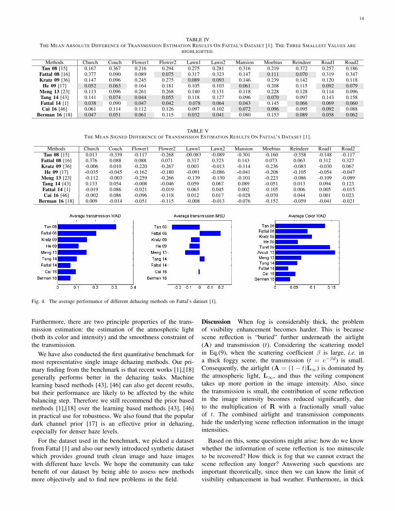
Dehazing results evaluation We evaluate the dehazing re-sults. The mean absolute difference (MAD) of each method(excluding sky regions) to the ground truth clean image arelisted in Table VI and the dehazing results on church caseare shown in Figure 5. In Table VI, the three smallest errorsfor each image are highlighted. Again, there is no one methodcan be outstanding for all cases. It is clear that the observednon-model based methods Tarel 09 [35] and Ancuti 13 [40]obtain largest error in the recovery. The visual qualities oftheir results are also rather inferior compared with othermethods (as can be seen in Figure 5). This shows that onlyimage contrast enhancement operation without the haze imagemodel Eq. (12) cannot achieve satisfactory results. Among the

13

rest model based methods, the latest methods Meng 13 [23],Tang 14 [43], Fattal 14 [1], Cai 16 [46], Berman 16 [18], andalso He 09 [17] generally perform better than early dehazingmethods Tan 08 [15], Fattal 08 [16], and Kratz 09 [36].Especially Fattal 14 [1] and Berman 16 [18] are the best twomethods that can provide dehazing results that are the mostclose to the ground truth. This quantification ranking reflectswell the visual quality as the example shown in Fig 5.

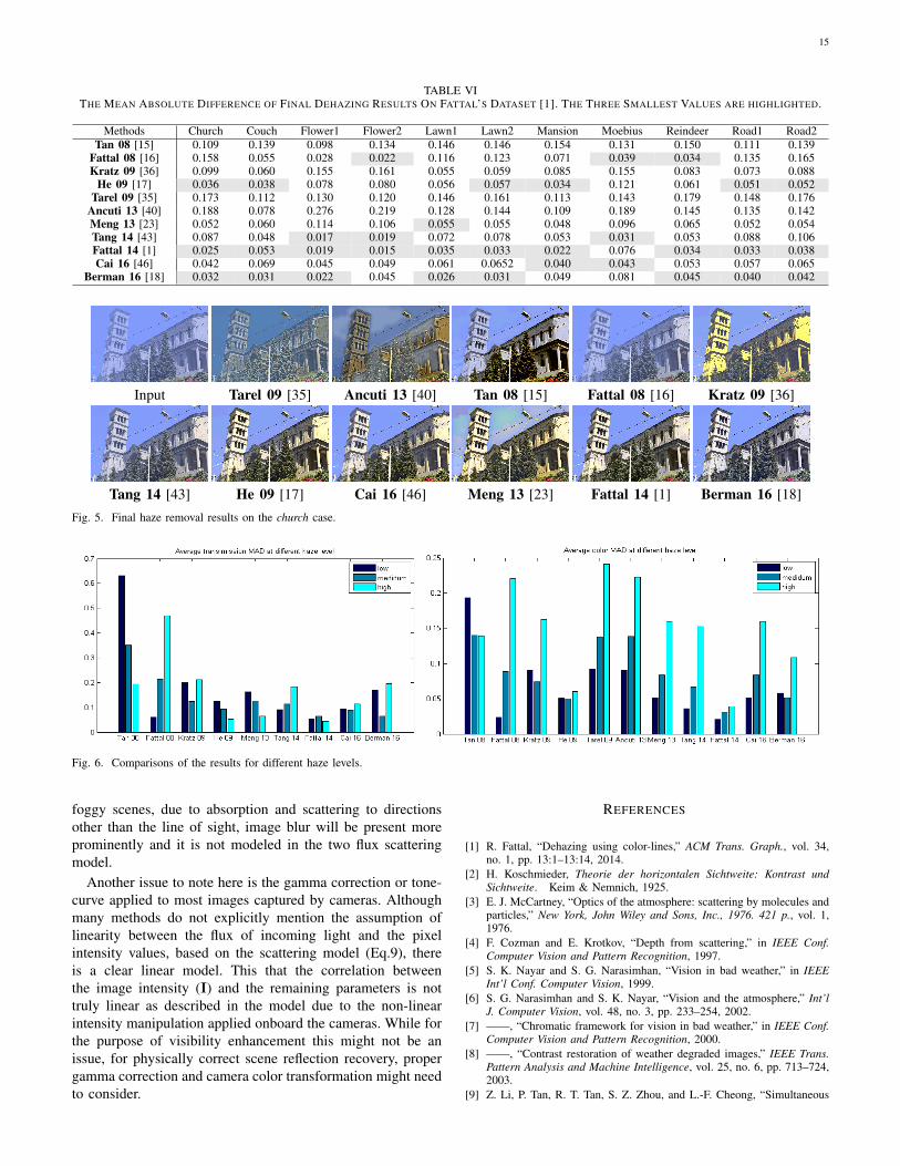
Evaluation with various haze levels Additionally, we testthe performance of each method for different haze levels. InFattal’s dataset [1], he provides a subset of images (lawn1,mansion, reindeer, road1) that are synthesized with threedifferent haze level by control the scattering coefficient β. Asβ increases, denser haze effects will appear. We measure thetransmission estimation error and final dehazing error usingthe mean absolute difference and the average results over allscenes are plotted in Figure 6.

It is clearly observed that Fattal 14 [1] stably stand out inachieving less errors in both transmission estimation and finaldehazing at different haze levels. Fattal 08 [16] works wellonly at low haze levels and the performance drops at mediumand high haze levels. Looking at the transmission results, wecan see Tan 08 [15], He 09 [17], and Meng 13 [23]’s estima-tion becomes more accurate when haze level increases. Thisdemonstrates the priors of these three methods are correlatedwith haze such that these priors can tell more informationwith more haze. The difference is that He 09 [17], and Meng13 [23] can achieve much smaller transmission errors than Tan08 [15], showing the superiority of dark channel prior [17]and boundary constrain [23] against the local contrast [15] forthis task. This can be explained by the fact that with heavierhaze, the contribution of the airlight A(x) increases, wheredark channel prior and boundary constraint assumption can fitmore.

Berman 16 [18] can achieve the least transmission estima-tion error at medium haze level but the error increases at bothlow and heavy haze levels. This may reveal one limitationof Berman 16 [18] that the haze lines formed from non localpixels work well only at certain haze levels. In near clean (lowhaze level) or heavily hazy scenarios, the haze lines found maynot be reliable. The two learning methods, Tang 14 [43] andCai 16 [46], predict the transmission decently well. For thefinal dehaze results, most methods obtain large error in heavyhaze except He 09 [17] and Fattal 14 [1].

B. Evaluation on our Dataset

Unlike the Fattal’s dataset that are generated using imagewith the haze image model Eq. (12), we generate our datasetusing a physically based rendering technique (PBRT) that usesthe Monte Carlo ray tracing in a volumetric scattering medium[50]. We render five sets of different scenes under differenthaze level of different types, namely swarp, house, building,island, villa. Our scenes are created using freely available 3Dmodels. All five scenes contains large depth variation from afew meters to about 2, 000 meters. We assume a uniform hazedensity in the space and use homogeneous volumes in ourrendering. For each of the five scenes, we render six images.

The first one is rendered with no participating media and isconsidered as the ground truth. The remaining five imagesare rendered with increasing haze level, namely, by evenlyincreasing the absorption coefficient σa and the scatteringcoefficient σs. Figure 7 shows two sets of our generatedsynthetic data (building, island). As can be seen, the visibilityof the scene, especially further away objects, decreases whenthe haze level increases. The whole dataset will be availablevia a project website.

We have evaluated 9 methods on our dataset (Fattal 08 [16]and Fattal 14 [1]’s results are not available on our dataset).We quantify the visibility enhancement outputs by comparingthem with their respective ground truths. The quantitativemeasurement is done by using the structural similarity index(SSIM) [51]. While MAD directly measure the closeness ofthe output to the ground truth pixel by pixel, SSIM is moreconsistent with human visual perception, especially in thecases of dehazing for heavier haze level. SSIM is a popularchoice to compute the structure similarity of two images inimage restoration tasks. Unlike MAD, a higher value in SSIMindicate a better match as it is a similarity measurement.

Figure 8 shows the performance of each method in term ofSSIM. It is observed that again latest methods Tang 14 [43],Cai 16 [46], and Berman 16 [18] generally performed betterthan others. He 09 [17] also performs very well, especially inheavier haze levels. This is consistent with our experiment inSection IV-A.

C. Qualitative results on real images

We have also list three qualitative examples of the dehazingresults on real hazy images by different methods (more visualcomparisons can be found in the previous dehazing papere.g. [1], [18]). The visual comparison here confirms ourfindings in the previous benchmarking that Fattal 14 [1]and Berman 16 [18] are the best two methods that canconsistently provide excellent dehazing results. Some earlymethods like Kratz 09 [36], Tarel 09 [35], Ancuti 13 [40]exhibit noticeable limitations in the dehazing results (e.g. over-saturation, boundary artifacts, color shift). The He 09 [17]and Meng 13 [23] also performs well and obtain similarresults as they essentially both predict the lower bound ofthe transmission. The results of the learning based methodTang 14 [43] and Cai 16 [46] can produce appealing resultsin general but usually tend to leave haze in results.

V. SUMMARY AND DISCUSSION

Summary This paper has provided a thorough surveyof major methods of visibility enhancement in hazy/foggyscenes. Various modalities such as multiple images, knownapproximated depth, stereo, and polarizing filters have beenintroduced to tackle the problem. Special emphasis was placedon single-image methods where significant image cues havebeen explored to enhance visibility, such as local contrast [15],shading-transmission decomposition [16], dark channel prior[17], line intersection [1] etc.. The tenet of all the methodsis to use scene cues to estimate light transmission and tounveil scene reflection based on the estimated transmission.

14

TABLE IVTHE MEAN ABSOLUTE DIFFERENCE OF TRANSMISSION ESTIMATION RESULTS ON FATTAL’S DATASET [1]. THE THREE SMALLEST VALUES ARE

HIGHLIGHTED.

Methods Church Couch Flower1 Flower2 Lawn1 Lawn2 Mansion Moebius Reindeer Road1 Road2Tan 08 [15] 0.167 0.367 0.216 0.294 0.275 0.281 0.316 0.219 0.372 0.257 0.186

Fattal 08 [16] 0.377 0.090 0.089 0.075 0.317 0.323 0.147 0.111 0.070 0.319 0.347Kratz 09 [36] 0.147 0.096 0.245 0.275 0.089 0.093 0.146 0.239 0.142 0.120 0.118

He 09 [17] 0.052 0.063 0.164 0.181 0.105 0.103 0.061 0.208 0.115 0.092 0.079Meng 13 [23] 0.113 0.096 0.261 0.268 0.140 0.131 0.118 0.228 0.128 0.114 0.096Tang 14 [43] 0.141 0.074 0.044 0.055 0.118 0.127 0.096 0.070 0.097 0.143 0.158Fattal 14 [1] 0.038 0.090 0.047 0.042 0.078 0.064 0.043 0.145 0.066 0.069 0.060Cai 16 [46] 0.061 0.114 0.112 0.126 0.097 0.102 0.072 0.096 0.095 0.092 0.088

Berman 16 [18] 0.047 0.051 0.061 0.115 0.032 0.041 0.080 0.153 0.089 0.058 0.062

TABLE VTHE MEAN SIGNED DIFFERENCE OF TRANSMISSION ESTIMATION RESULTS ON FATTAL’S DATASET [1].

Methods Church Couch Flower1 Flower2 Lawn1 Lawn2 Mansion Moebius Reindeer Road1 Road2Tan 08 [15] 0.013 -0.339 -0.117 -0.268 -00.083 -0.089 -0.301 -0.160 -0.358 -0.148 -0.117

Fattal 08 [16] 0.376 0.088 0.088 0.071 0.317 0.323 0.143 0.073 0.063 0.312 0.327Kratz 09 [36] -0.006 0.010 -0.220 -0.267 0.003 -0.013 -0.114 -0.236 -0.083 -0.030 0.067

He 09 [17] -0.035 -0.045 -0.162 -0.180 -0.091 -0.086 -0.041 -0.208 -0.105 -0.054 -0.047Meng 13 [23] -0.112 -0.003 -0.259 -0.266 -0.139 -0.130 -0.101 -0.223 -0.086 -0.109 -0.089Tang 14 [43] 0.133 0.054 -0.008 -0.046 0.059 0.067 0.089 -0.051 0.013 0.094 0.123Fattal 14 [1] -0.019 0.086 -0.021 -0.019 0.063 0.045 0.002 -0.105 0.006 0.005 -0.015Cai 16 [46] -0.002 0.086 -0.096 -0.118 0.012 0.017 -0.028 -0.070 0.044 0.001 0.023

Berman 16 [18] 0.009 -0.014 -0.051 -0.115 -0.008 -0.013 -0.076 -0.152 -0.059 -0.041 -0.021

Fig. 4. The average performance of different dehazing methods on Fattal’s dataset [1].

Furthermore, there are two principle properties of the trans-mission estimation: the estimation of the atmospheric light(both its color and intensity) and the smoothness constraint ofthe transmission.

We have also conducted the first quantitative benchmark formost representative single image dehazing methods. Our pri-mary finding from the benchmark is that recent works [1],[18]generally performs better in the dehazing tasks. Machinelearning based methods [43], [46] can also get decent results,but their performance are likely to be affected by the whitebalancing step. Therefore we still recommend the prior basedmethods [1],[18] over the learning based methods [43], [46]in practical use for robustness. We also found that the populardark channel prior [17] is an effective prior in dehazing,especially for denser haze levels.

For the dataset used in the benchmark, we picked a datasetfrom Fattal [1] and also our newly introduced synthetic datasetwhich provides ground truth clean image and haze imageswith different haze levels. We hope the community can takebenefit of our dataset by being able to assess new methodsmore objectively and to find new problems in the field.

Discussion When fog is considerably thick, the problemof visibility enhancement becomes harder. This is becausescene reflection is “buried” further underneath the airlight(A) and transmission (t). Considering the scattering modelin Eq.(9), when the scattering coefficient β is large, i.e. ina thick foggy scene, the transmission (t = e−βd) is small.Consequently, the airlight (A = (1− t)L∞) is dominated bythe atmospheric light, L∞, and thus the veiling componenttakes up more portion in the image intensity. Also, sincethe transmission is small, the contribution of scene reflectionin the image intensity becomes reduced significantly, dueto the multiplication of R with a fractionally small valueof t. The combined airlight and transmission componentshide the underlying scene reflection information in the imageintensities.

Based on this, some questions might arise: how do we knowwhether the information of scene reflection is too minusculeto be recovered? How thick is fog that we cannot extract thescene reflection any longer? Answering such questions areimportant theoretically, since then we can know the limit ofvisibility enhancement in bad weather. Furthermore, in thick

15

TABLE VITHE MEAN ABSOLUTE DIFFERENCE OF FINAL DEHAZING RESULTS ON FATTAL’S DATASET [1]. THE THREE SMALLEST VALUES ARE HIGHLIGHTED.

Methods Church Couch Flower1 Flower2 Lawn1 Lawn2 Mansion Moebius Reindeer Road1 Road2Tan 08 [15] 0.109 0.139 0.098 0.134 0.146 0.146 0.154 0.131 0.150 0.111 0.139

Fattal 08 [16] 0.158 0.055 0.028 0.022 0.116 0.123 0.071 0.039 0.034 0.135 0.165Kratz 09 [36] 0.099 0.060 0.155 0.161 0.055 0.059 0.085 0.155 0.083 0.073 0.088

He 09 [17] 0.036 0.038 0.078 0.080 0.056 0.057 0.034 0.121 0.061 0.051 0.052Tarel 09 [35] 0.173 0.112 0.130 0.120 0.146 0.161 0.113 0.143 0.179 0.148 0.176

Ancuti 13 [40] 0.188 0.078 0.276 0.219 0.128 0.144 0.109 0.189 0.145 0.135 0.142Meng 13 [23] 0.052 0.060 0.114 0.106 0.055 0.055 0.048 0.096 0.065 0.052 0.054Tang 14 [43] 0.087 0.048 0.017 0.019 0.072 0.078 0.053 0.031 0.053 0.088 0.106Fattal 14 [1] 0.025 0.053 0.019 0.015 0.035 0.033 0.022 0.076 0.034 0.033 0.038Cai 16 [46] 0.042 0.069 0.045 0.049 0.061 0.0652 0.040 0.043 0.053 0.057 0.065

Berman 16 [18] 0.032 0.031 0.022 0.045 0.026 0.031 0.049 0.081 0.045 0.040 0.042

Input Tarel 09 [35] Ancuti 13 [40] Tan 08 [15] Fattal 08 [16] Kratz 09 [36]

Tang 14 [43] He 09 [17] Cai 16 [46] Meng 13 [23] Fattal 14 [1] Berman 16 [18]

Fig. 5. Final haze removal results on the church case.

Fig. 6. Comparisons of the results for different haze levels.

foggy scenes, due to absorption and scattering to directionsother than the line of sight, image blur will be present moreprominently and it is not modeled in the two flux scatteringmodel.

Another issue to note here is the gamma correction or tone-curve applied to most images captured by cameras. Althoughmany methods do not explicitly mention the assumption oflinearity between the flux of incoming light and the pixelintensity values, based on the scattering model (Eq.9), thereis a clear linear model. This that the correlation betweenthe image intensity (I) and the remaining parameters is nottruly linear as described in the model due to the non-linearintensity manipulation applied onboard the cameras. While forthe purpose of visibility enhancement this might not be anissue, for physically correct scene reflection recovery, propergamma correction and camera color transformation might needto consider.

REFERENCES

[1] R. Fattal, “Dehazing using color-lines,” ACM Trans. Graph., vol. 34,no. 1, pp. 13:1–13:14, 2014.

[2] H. Koschmieder, Theorie der horizontalen Sichtweite: Kontrast undSichtweite. Keim & Nemnich, 1925.

[3] E. J. McCartney, “Optics of the atmosphere: scattering by molecules andparticles,” New York, John Wiley and Sons, Inc., 1976. 421 p., vol. 1,1976.

[4] F. Cozman and E. Krotkov, “Depth from scattering,” in IEEE Conf.Computer Vision and Pattern Recognition, 1997.

[5] S. K. Nayar and S. G. Narasimhan, “Vision in bad weather,” in IEEEInt’l Conf. Computer Vision, 1999.

[6] S. G. Narasimhan and S. K. Nayar, “Vision and the atmosphere,” Int’lJ. Computer Vision, vol. 48, no. 3, pp. 233–254, 2002.

[7] ——, “Chromatic framework for vision in bad weather,” in IEEE Conf.Computer Vision and Pattern Recognition, 2000.

[8] ——, “Contrast restoration of weather degraded images,” IEEE Trans.Pattern Analysis and Machine Intelligence, vol. 25, no. 6, pp. 713–724,2003.

[9] Z. Li, P. Tan, R. T. Tan, S. Z. Zhou, and L.-F. Cheong, “Simultaneous

16

Fig. 7. Samples of our synthetic data with increasing haze levels.

Fig. 8. The performance of each method on our dataset on 5 haze levels (l=1,2,3,4,5, low to high) in term of SSIM.

video defogging and stereo reconstruction,” in IEEE Conf. ComputerVision and Pattern Recognition, 2015.

[10] Y. Y. Schechner, S. G. Narasimhan, and S. K. Nayar, “Instant dehazing ofimages using polarization,” in IEEE Conf. Computer Vision and PatternRecognition, 2001.

[11] S. Shwartz, E. Namer, and Y. Y. Schechner, “Blind haze separation,” inIEEE Conf. Computer Vision and Pattern Recognition, 2006.

[12] J. P. Oakley and B. L. Satherley, “Improving image quality in poorvisibility conditions using a physical model for contrast degradation,”IEEE Trans. Image Processing, vol. 7, no. 2, pp. 167–179, 1998.

[13] N. Hautiere, J.-P. Tarel, and D. Aubert, “Towards fog-free in-vehiclevision systems through contrast restoration,” in IEEE Conf. ComputerVision and Pattern Recognition, 2007.

[14] J. Kopf, B. Neubert, B. Chen, M. F. Cohen, D. Cohen-Or, O. Deussen,M. Uyttendaele, and D. Lischinski, “Deep photo: Model-based photo-graph enhancement and viewing,” ACM Trans. Graphics, vol. 27, no. 5,pp. 116:1–116:10, 2008.

[15] R. T. Tan, “Visibility in bad weather from a single image,” in IEEEConf. Computer Vision and Pattern Recognition, 2008.

[16] R. Fattal, “Single image dehazing,” ACM Trans. Graphics, vol. 27, no. 3,p. 72, 2008.

[17] K. He, J. Sun, and X. Tang, “Single image haze removal using darkchannel prior,” in IEEE Conf. Computer Vision and Pattern Recognition,2009.

[18] D. Berman, T. Treibitz, and S. Avidan, “Non-local image dehazing,” inIEEE Conf. Computer Vision and Pattern Recognition, 2016.

[19] G. M. Hidy and M. Kerker, Aerosols and Atmospheric Chemistry: TheKendall Award Symposium Honoring Milton Kerker, at the Proceedingsof the American Chemical Society, Los Angeles, California, March 28-April 2, 1971. Academic Press, 1972.

[20] M. O. Codes, “International codes–wmo no. 306,” Geneva–Switzerland:World Meteorological, 1995.

[21] C. D. Ahrens, Meteorology today: an introduction to weather, climate,and the environment. West Publishing Company New York, 1991.

[22] M. G. J. Minnaert, The Nature of Light and Colour in the Open Air:Transl.[By] HM Krener-Priest, Rev.[By] KE Brian Jay. Dover, 1954.

[23] G. Meng, Y. Wang, J. Duan, S. Xiang, and C. Pan, “Efficient imagedehazing with boundary constraint and contextual regularization,” inIEEE Int’l Conf. Computer Vision, 2013.

[24] S. A. Shafer, “Using color to separate reflection components,” ColorResearch & Application, vol. 10, no. 4, pp. 210–218, 1985.

[25] G. J. Klinker, S. A. Shafer, and T. Kanade, “A physical approach tocolor image understanding,” Int’l J. Computer Vision, vol. 4, no. 1, pp.7–38, 1990.

[26] S. Tominaga and B. A. Wandell, “Standard surface-reflectance modeland illuminant estimation,” J. Opt. Soc. Am. A, vol. 6, no. 4, pp. 576–584, 1989.

[27] L. Caraffa and J.-P. Tarel, “Stereo reconstruction and contrast restorationin daytime fog,” in Asian Conf. Computer Vision, 2012.

[28] G. Zhang, J. Jia, T.-T. Wong, and H. Bao, “Consistent depth mapsrecovery from a video sequence,” IEEE Trans. Pattern Analysis andMachine Intelligence, vol. 31, no. 6, pp. 974–988, 2009.

[29] K. Tan and J. P. Oakley, “Enhancement of color images in poor visibilityconditions,” in IEEE Int’l Conf. Image Processing, 2000.

[30] S. G. Narasimhan and S. K. Nayar, “Interactive (de) weathering ofan image using physical models,” in IEEE Workshop on Color andPhotometric Methods in Computer Vision, 2003.

[31] R. T. Tan, N. Pettersson, and L. Petersson, “Visibility enhancementfor roads with foggy or hazy scenes,” in IEEE Intelligent VehiclesSymposium, 2007.

[32] R. T. Tan, K. Nishino, and K. Ikeuchi, “Color constancy through inverse-intensity chromaticity space,” J. Opt. Soc. Am. A, vol. 21, no. 3, pp.321–334, 2004.

[33] K. He, J. Sun, and X. Tang, “Single image haze removal using darkchannel prior,” IEEE Trans. Pattern Analysis and Machine Intelligence,vol. 33, no. 12, pp. 2341–2353, 2011.

[34] A. Levin, D. Lischinski, and Y. Weiss, “A closed-form solution to naturalimage matting,” IEEE Trans. Pattern Analysis and Machine Intelligence,vol. 30, no. 2, pp. 228–242, 2008.

[35] J.-P. Tarel and N. Hautiere, “Fast visibility restoration from a singlecolor or gray level image,” in IEEE Int’l Conf. Computer Vision, 2009.

[36] L. Kratz and K. Nishino, “Factorizing scene albedo and depth from asingle foggy image,” in IEEE Int’l Conf. Computer Vision, 2009.

[37] K. Nishino, L. Kratz, and S. Lombardi, “Bayesian defogging,” Int’l J.Computer Vision, vol. 98, no. 3, pp. 263–278, 2012.

[38] J. Kim and R. Zabih, “Factorial markov random fields,” in EuropeanConf. Computer Vision, 2002.

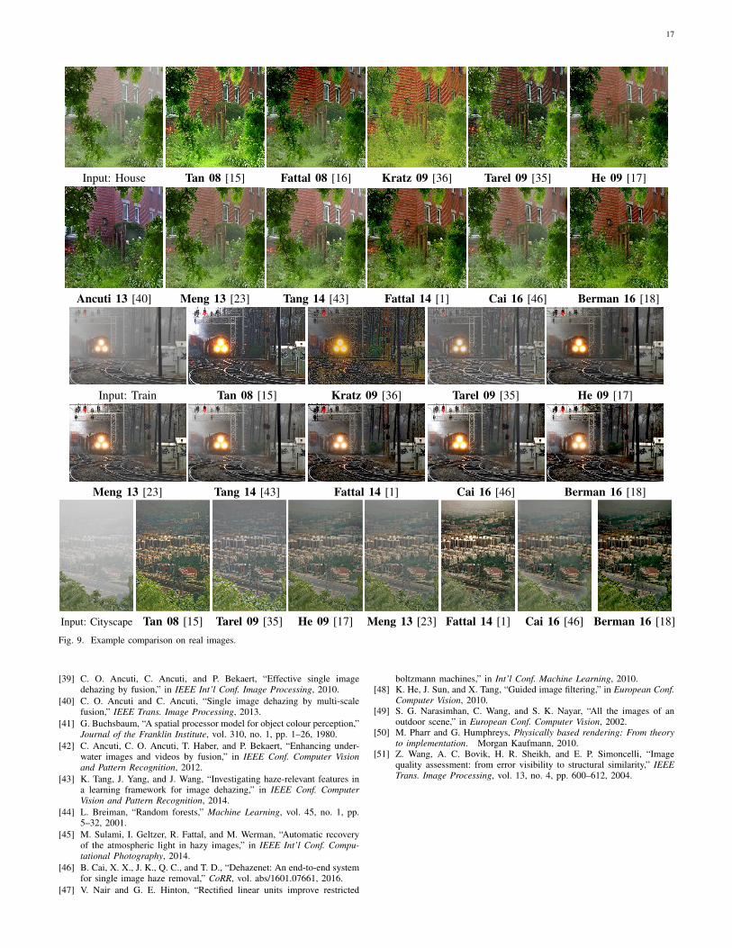
17

Input: House Tan 08 [15] Fattal 08 [16] Kratz 09 [36] Tarel 09 [35] He 09 [17]

Ancuti 13 [40] Meng 13 [23] Tang 14 [43] Fattal 14 [1] Cai 16 [46] Berman 16 [18]

Input: Train Tan 08 [15] Kratz 09 [36] Tarel 09 [35] He 09 [17]

Meng 13 [23] Tang 14 [43] Fattal 14 [1] Cai 16 [46] Berman 16 [18]

Input: Cityscape Tan 08 [15] Tarel 09 [35] He 09 [17] Meng 13 [23] Fattal 14 [1] Cai 16 [46] Berman 16 [18]Fig. 9. Example comparison on real images.

[39] C. O. Ancuti, C. Ancuti, and P. Bekaert, “Effective single imagedehazing by fusion,” in IEEE Int’l Conf. Image Processing, 2010.

[40] C. O. Ancuti and C. Ancuti, “Single image dehazing by multi-scalefusion,” IEEE Trans. Image Processing, 2013.

[41] G. Buchsbaum, “A spatial processor model for object colour perception,”Journal of the Franklin Institute, vol. 310, no. 1, pp. 1–26, 1980.

[42] C. Ancuti, C. O. Ancuti, T. Haber, and P. Bekaert, “Enhancing under-water images and videos by fusion,” in IEEE Conf. Computer Visionand Pattern Recognition, 2012.

[43] K. Tang, J. Yang, and J. Wang, “Investigating haze-relevant features ina learning framework for image dehazing,” in IEEE Conf. ComputerVision and Pattern Recognition, 2014.

[44] L. Breiman, “Random forests,” Machine Learning, vol. 45, no. 1, pp.5–32, 2001.

[45] M. Sulami, I. Geltzer, R. Fattal, and M. Werman, “Automatic recoveryof the atmospheric light in hazy images,” in IEEE Int’l Conf. Compu-tational Photography, 2014.

[46] B. Cai, X. X., J. K., Q. C., and T. D., “Dehazenet: An end-to-end systemfor single image haze removal,” CoRR, vol. abs/1601.07661, 2016.

[47] V. Nair and G. E. Hinton, “Rectified linear units improve restricted

boltzmann machines,” in Int’l Conf. Machine Learning, 2010.[48] K. He, J. Sun, and X. Tang, “Guided image filtering,” in European Conf.

Computer Vision, 2010.[49] S. G. Narasimhan, C. Wang, and S. K. Nayar, “All the images of an

outdoor scene,” in European Conf. Computer Vision, 2002.[50] M. Pharr and G. Humphreys, Physically based rendering: From theory

to implementation. Morgan Kaufmann, 2010.[51] Z. Wang, A. C. Bovik, H. R. Sheikh, and E. P. Simoncelli, “Image

quality assessment: from error visibility to structural similarity,” IEEETrans. Image Processing, vol. 13, no. 4, pp. 600–612, 2004.