hatchet documentation - hatchet.readthedocs.io

hatchet Documentation

Abhinav Bhatele

May 01, 2021

User Docs

1 Getting Started 31.1 Prerequisites . . . . . . . . . . . . . . . . . . . . . . . . . . . . . . . . . . . . . . . . . . . . . . . 31.2 Installation . . . . . . . . . . . . . . . . . . . . . . . . . . . . . . . . . . . . . . . . . . . . . . . . 31.3 Supported data formats . . . . . . . . . . . . . . . . . . . . . . . . . . . . . . . . . . . . . . . . . . 4

2 User Guide 52.1 Data structures in hatchet . . . . . . . . . . . . . . . . . . . . . . . . . . . . . . . . . . . . . . . . 52.2 Reading in a dataset . . . . . . . . . . . . . . . . . . . . . . . . . . . . . . . . . . . . . . . . . . . 62.3 Visualizing the data . . . . . . . . . . . . . . . . . . . . . . . . . . . . . . . . . . . . . . . . . . . 62.4 Dataframe operations . . . . . . . . . . . . . . . . . . . . . . . . . . . . . . . . . . . . . . . . . . . 82.5 Graph operations . . . . . . . . . . . . . . . . . . . . . . . . . . . . . . . . . . . . . . . . . . . . . 102.6 GraphFrame operations . . . . . . . . . . . . . . . . . . . . . . . . . . . . . . . . . . . . . . . . . 11

3 Analysis Examples 133.1 Reading different file formats . . . . . . . . . . . . . . . . . . . . . . . . . . . . . . . . . . . . . . 133.2 Basic Examples . . . . . . . . . . . . . . . . . . . . . . . . . . . . . . . . . . . . . . . . . . . . . 193.3 Scaling Performance Examples . . . . . . . . . . . . . . . . . . . . . . . . . . . . . . . . . . . . . 23

4 Basic Tutorial: Hatchet 101 294.1 Installing Hatchet and Tutorial Setup . . . . . . . . . . . . . . . . . . . . . . . . . . . . . . . . . . 294.2 Introduction . . . . . . . . . . . . . . . . . . . . . . . . . . . . . . . . . . . . . . . . . . . . . . . 304.3 Analyzing the DataFrame using pandas . . . . . . . . . . . . . . . . . . . . . . . . . . . . . . . . . 314.4 Analyzing the Graph via printing . . . . . . . . . . . . . . . . . . . . . . . . . . . . . . . . . . . . 314.5 Analyzing the GraphFrame . . . . . . . . . . . . . . . . . . . . . . . . . . . . . . . . . . . . . . . 354.6 Analyzing Multiple GraphFrames . . . . . . . . . . . . . . . . . . . . . . . . . . . . . . . . . . . . 37

5 Publications and Presentations 395.1 Publications . . . . . . . . . . . . . . . . . . . . . . . . . . . . . . . . . . . . . . . . . . . . . . . 395.2 Posters . . . . . . . . . . . . . . . . . . . . . . . . . . . . . . . . . . . . . . . . . . . . . . . . . . 395.3 Tutorials . . . . . . . . . . . . . . . . . . . . . . . . . . . . . . . . . . . . . . . . . . . . . . . . . 39

6 hatchet package 416.1 Subpackages . . . . . . . . . . . . . . . . . . . . . . . . . . . . . . . . . . . . . . . . . . . . . . . 416.2 Submodules . . . . . . . . . . . . . . . . . . . . . . . . . . . . . . . . . . . . . . . . . . . . . . . 446.3 hatchet.frame module . . . . . . . . . . . . . . . . . . . . . . . . . . . . . . . . . . . . . . . . . . 446.4 hatchet.graph module . . . . . . . . . . . . . . . . . . . . . . . . . . . . . . . . . . . . . . . . . . 456.5 hatchet.graphframe module . . . . . . . . . . . . . . . . . . . . . . . . . . . . . . . . . . . . . . . 46

i

6.6 hatchet.node module . . . . . . . . . . . . . . . . . . . . . . . . . . . . . . . . . . . . . . . . . . . 496.7 hatchet.query_matcher module . . . . . . . . . . . . . . . . . . . . . . . . . . . . . . . . . . . . . . 516.8 Module contents . . . . . . . . . . . . . . . . . . . . . . . . . . . . . . . . . . . . . . . . . . . . . 51

7 Indices and tables 53

Python Module Index 55

Index 57

ii


Hatchet is a Python-based library that allows Pandas dataframes to be indexed by structured tree and graph data. Itis intended for analyzing performance data that has a hierarchy (for example, serial or parallel profiles that representcalling context trees, call graphs, nested regions’ timers, etc.). Hatchet implements various operations to analyze asingle hierarchical data set or compare multiple data sets, and its API facilitates analyzing such data programmatically.

You can get hatchet from its GitHub repository:

$ git clone https://github.com/LLNL/hatchet.git

or install it using pip:

$ pip install hatchet

If you are new to hatchet and want to start using it, see Getting Started, or refer to the full User Guide below.

User Docs 1

https://pandas.pydata.org

https://github.com/LLNL/hatchet


2 User Docs

CHAPTER 1

Getting Started

1.1 Prerequisites

Hatchet has the following minimum requirements, which must be installed before Hatchet is run:

1. Python 2 (2.7) or 3 (3.5 - 3.8)

2. matplotlib

3. pydot

4. numpy, and

5. pandas

Hatchet is available on GitHub.

1.2 Installation

You can get hatchet from its GitHub repository using this command:


This will create a directory called hatchet.

1.2.1 Install and Build Hatchet

To build hatchet and update your PYTHONPATH, run the following shell script from the hatchet root directory:

$ source ./install.sh

Note: The source keyword is required to update your PYTHONPATH environment variable. It is not necessary ifyou have already manually added the hatchet directory to your PYTHONPATH.

3




Alternatively, you can install hatchet using pip:


1.2.2 Check Installation

After installing hatchet, you should be able to import hatchet when running the Python interpreter in interactive mode:

$ pythonPython 3.7.4 (default, Jul 11 2019, 01:08:00)[Clang 10.0.1 (clang-1001.0.46.4)] on darwinType "help", "copyright", "credits" or "license" for more information.>>>

Typing import hatchet at the prompt should succeed without any error messages:

>>> import hatchet>>>

1.3 Supported data formats

Currently, hatchet supports the following data formats as input:

• HPCToolkit database: This is generated by using hpcprof-mpi to post-process the raw measurements direc-tory output by HPCToolkit.

• Caliper Cali file: This is the format in which caliper outputs raw performance data by default.

• Caliper Json-split file: This is generated by either running cali-query on the raw caliper data or by enabling thempireport service when using caliper.

• DOT format: This is generated by using gprof2dot on gprof or callgrind output.

• String literal: Hatchet can read as input a list of dictionaries that represents a graph.

• List: Hatchet can also read a list of lists that represents a graph.

For more details on the different input file formats, refer to the User Guide.

4 Chapter 1. Getting Started

http://hpctoolkit.org/index.html

http://llnl.github.io/Caliper/OutputFormats.html#cali

http://llnl.github.io/Caliper/OutputFormats.html#json-split

https://www.graphviz.org/doc/info/lang.html

https://github.com/jrfonseca/gprof2dot

CHAPTER 2

User Guide

Hatchet is a Python tool that simplifies the process of analyzing hierarchical performance data such as calling contexttrees. Hatchet uses pandas dataframes to store the data on each node of the hierarchy and keeps the graph relationshipsbetween the nodes in a different data structure that is kept consistent with the dataframe.

2.1 Data structures in hatchet

Hatchet’s primary data structure is a GraphFrame, which combines a structured index in the form of a graph witha pandas dataframe. The images on the right show the two objects in a GraphFrame – a Graph object (the index),and a DataFrame object storing the metrics associated with each node.

Graphframe stores the performance data that is read in from an HPCToolkit database, Caliper Json or Cali file, orgprof/callgrind DOT file. Typically, the raw input data is in the form of a tree. However, since subsequent operationson the tree can lead to new edges being created which can turn the tree into a graph, we store the input data as a directedgraph. The graphframe consists of a graph object that stores the edge relationships between nodes and a dataframethat stores different metrics (numerical data) and categorical data associated with each node.

5


Graph: The graph can be connected or disconnected (multiple roots) and each node in the graph can have one ormore parents and children. The node stores its frame, which can be defined by the reader. The callpath is derived byappending the frames from the root to a given node.

Dataframe: The dataframe holds all the numerical and categorical data associated with each node. Since typically thecall tree data is per process, a multiindex composed of the node and MPI rank is used to index into the dataframe.

2.2 Reading in a dataset

One can use one of several static methods defined in the GraphFrame class to read in an input dataset usinghatchet. For example, if a user has an HPCToolkit database directory that they want to analyze, they can use thefrom_hpctoolkit method:

import hatchet as ht

if __name__ == "__main__":dirname = "hatchet/tests/data/hpctoolkit-cpi-database"gf = ht.GraphFrame.from_hpctoolkit(dirname)

Similarly if the input file is a split-JSON output by Caliper, they can use the from_caliper_json method:


if __name__ == "__main__":filename = ("hatchet/tests/data/caliper-lulesh-json/lulesh-sample-annotation-

→˓profile.json")gf = ht.GraphFrame.from_caliper_json(filename)

Examples of reading in other file formats can be found in Analysis Examples.

2.3 Visualizing the data

6 Chapter 2. User Guide


When the graph represented by the input dataset is small, the user may be interested in visualizing it in entirety ora portion of it. Hatchet provides several mechanisms to visualize the graph in hatchet. One can use the tree()function to convert the graph into a string that can be printed on standard output:

print(gf.tree())

One can also use the to_dot() function to output the tree as a string in the Graphviz’ DOT format. This can bewritten to a file and then used to display a tree using the dot or neato program.

with open("test.dot", "w") as dot_file:dot_file.write(gf.to_dot())

$ dot -Tpdf test.dot > test.pdf

One can also use the to_flamegraph function to output the tree as a string in the folded stack format required byflamegraph. This file can then be used to create a flamegraph using flamegraph.pl.

with open("test.txt", "w") as folded_stack:folded_stack.write(gf.to_flamegraph())

$ ./flamegraph.pl test.txt > test.svg

One can also print the contents of the dataframe to standard output:

pd.set_option("display.width", 1200)pd.set_option("display.max_colwidth", 20)pd.set_option("display.max_rows", None)

print(gf.dataframe)

If there are many processes or threads in the dataframe, one can also print a cross section of the dataframe, say thevalues for rank 0, like this:

2.3. Visualizing the data 7


print(gf.dataframe.xs(0, level="rank"))

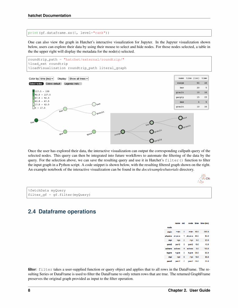
One can also view the graph in Hatchet’s interactive visualization for Jupyter. In the Jupyter visualization shownbelow, users can explore their data by using their mouse to select and hide nodes. For those nodes selected, a table inthe the upper right will display the metadata for the node(s) selected.

roundtrip_path = "hatchet/external/roundtrip/"%load_ext roundtrip%loadVisualization roundtrip_path literal_graph

Once the user has explored their data, the interactive visualization can output the corresponding callpath query of theselected nodes. This query can then be integrated into future workflows to automate the filtering of the data by thequery. For the selection above, we can save the resulting query and use it in Hatchet’s filter() function to filterthe input graph in a Python script. A code snippet is shown below, with the resulting filtered graph shown on the right.An example notebook of the interactive visualization can be found in the docs/examples/tutorials directory.

%fetchData myQueryfilter_gf = gf.filter(myQuery)

2.4 Dataframe operations

filter: filter takes a user-supplied function or query object and applies that to all rows in the DataFrame. The re-sulting Series or DataFrame is used to filter the DataFrame to only return rows that are true. The returned GraphFramepreserves the original graph provided as input to the filter operation.



filtered_gf = gf.filter(lambda x: x['time'] > 10.0)

The images on the right show a DataFrame before and after a filter operation.

An alternative way to filter the DataFrame is to supply a query path in the form of a query object. A query object is alist of abstract graph nodes that specifies a call path pattern to search for in the GraphFrame. An abstract graph nodeis made up of two parts:

• A wildcard that specifies the number of real nodes to match to the abstract node. This is represented as either astring with value “.” (match one node), “*” (match zero or more nodes), or “+” (match one or more nodes) or aninteger (match exactly that number of nodes). By default, the wildcard is “.” (or 1).

• A filter that is used to determine whether a real node matches the abstract node. In the high-level API, this isrepresented as a Python dictionary keyed on column names from the DataFrame. By default, the filter is an“always true” filter (represented as an empty dictionary).

The query object is represented as a Python list of abstract nodes. To specify both parts of an abstract node, use a tuplewith the first element being the wildcard and the second element being the filter. To use a default value for either thewildcard or the filter, simply provide the other part of the abstract node on its own (no need for a tuple). The user mustprovide at least one of the parts of the above definition of an abstract node.

The query language example below looks for all paths that match first a single node with name solvers, followed by 0or more nodes with an inclusive time greater than 10, followed by a single node with name that starts with p and endsin an integer and has an inclusive time greater than or equal to 10. When the query is used to filter and squash the thegraph shown on the right, the returned GraphFrame contains the nodes shown in the table on the right.

2.4. Dataframe operations 9


Filter is one of the operations that leads to the graph object and DataFrame object becoming inconsistent. After a filteroperation, there are nodes in the graph that do not return any rows when used to index into the DataFrame. Typically,the user will perform a squash on the GraphFrame after a filter operation to make the graph and DataFrame objectsconsistent again. This can be done either by manually calling the squash function on the new GraphFrame or bysetting the squash parameter of the filter function to True.

query = [{"name": "solvers"},("*", {"time (inc)": "> 10"}),{"name": "p[a-z]+[0-9]", "time (inc)": ">= 10"}

]

filtered_gf = gf.filter(query)

drop_index_levels: When there is per-MPI process or per-thread data in the DataFrame, a user might be interestedin aggregating the data in some fashion to analyze the graph at a coarser granularity. This function allows the user todrop the additional index columns in the hierarchical index by specifying an aggregation function. Essentially, thisperforms a groupby and aggregate operation on the DataFrame. The user-supplied function is used to performthe aggregation over all MPI processes or threads at the per-node granularity.

gf.drop_index_levels(function=np.max)

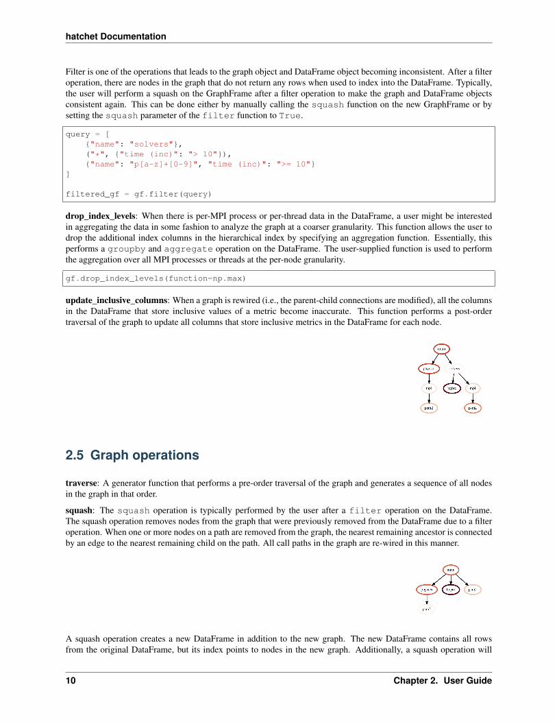
update_inclusive_columns: When a graph is rewired (i.e., the parent-child connections are modified), all the columnsin the DataFrame that store inclusive values of a metric become inaccurate. This function performs a post-ordertraversal of the graph to update all columns that store inclusive metrics in the DataFrame for each node.

2.5 Graph operations

traverse: A generator function that performs a pre-order traversal of the graph and generates a sequence of all nodesin the graph in that order.

squash: The squash operation is typically performed by the user after a filter operation on the DataFrame.The squash operation removes nodes from the graph that were previously removed from the DataFrame due to a filteroperation. When one or more nodes on a path are removed from the graph, the nearest remaining ancestor is connectedby an edge to the nearest remaining child on the path. All call paths in the graph are re-wired in this manner.

A squash operation creates a new DataFrame in addition to the new graph. The new DataFrame contains all rowsfrom the original DataFrame, but its index points to nodes in the new graph. Additionally, a squash operation will



make the values in all columns containing inclusive metrics inaccurate, since the parent-child relationships havechanged. Hence, the squash operation also calls update_inclusive_columns to make all inclusive columns inthe DataFrame accurate again.

filtered_gf = gf.filter(lambda x: x['time'] > 10.0)squashed_gf = filtered_gf.squash()

equal: The == operation checks whether two graphs have the same nodes and edge connectivity when traversing fromtheir roots. If they are equivalent, it returns true, otherwise it returns false.

union: The union function takes two graphs and creates a unified graph, preserving all edges structure of the originalgraphs, and merging nodes with identical context. When Hatchet performs binary operations on two GraphFrames withunequal graphs, a union is performed beforehand to ensure that the graphs are structurally equivalent. This ensuresthat operands to element-wise operations like add and subtract, can be aligned by their respective nodes.

2.6 GraphFrame operations

copy: The copy operation returns a shallow copy of a GraphFrame. It creates a new GraphFrame with a copy ofthe original GraphFrame’s DataFrame, but the same graph. As mentioned earlier, graphs in Hatchet use immutablesemantics, and they are copied only when they need to be restructured. This property allows us to reuse graphs fromGraphFrame to GraphFrame if the operations performed on the GraphFrame do not mutate the graph.

deepcopy: The deepcopy operation returns a deep copy of a GraphFrame. It is similar to copy, but returns a newGraphFrame with a copy of the original GraphFrame’s DataFrame and a copy of the original GraphFrame’s graph.

unify: unify operates on GraphFrames, and calls union on the two graphs, and then reindexes the DataFrames inboth GraphFrames to be indexed by the nodes in the unified graph. Binary operations on GraphFrames call unifywhich in turn calls union on the respective graphs.

add: Assuming the graphs in two GraphFrames are equal, the add (+) operation computes the element-wise sumof two DataFrames. In the case where the two graphs are not identical, unify (described above) is applied first tocreate a unified graph before performing the sum. The DataFrames are copied and reindexed by the combined graph,and the add operation returns new GraphFrame with the result of adding these DataFrames. Hatchet also provides anin-place version of the add operator: +=.

subtract: The subtract operation is similar to the add operation in that it requires the two graphs to be identical. Itapplies union and reindexes DataFrames if necessary. Once the graphs are unified, the subtract operation computesthe element-wise difference between the two DataFrames. The subtract operation returns a new GraphFrame, or itmodifies one of the GraphFrames in place in the case of the in-place subtraction (-=).

gf1 = ht.GraphFrame.from_literal( ... )gf2 = ht.GraphFrame.from_literal( ... )gf2 -= gf1

- =

tree: The tree operation returns the graphframe’s graph structure as a string that can be printed to the console.By default, the tree uses the name of each node and the associated time metric as the string representation. Thisoperation uses automatic color by default, but True or False can be used to force override.

2.6. GraphFrame operations 11

CHAPTER 3

Analysis Examples

3.1 Reading different file formats

Hatchet can read in a variety of data file formats into a GraphFrame. Below, we show examples of reading in differentdata formats.

3.1.1 Read in an HPCToolkit database

A database directory is generated by using hpcprof-mpi to post-process the raw measurements directory output byHPCToolkit. To analyze an HPCToolkit database, the from_hpctoolkit method can be used.

#!/usr/bin/env python


if __name__ == "__main__":# Path to HPCToolkit database directory.dirname = "../../../hatchet/tests/data/hpctoolkit-cpi-database"

# Use hatchet's ``from_hpctoolkit`` API to read in the HPCToolkit database.# The result is stored into Hatchet's GraphFrame.gf = ht.GraphFrame.from_hpctoolkit(dirname)

# Printout the DataFrame component of the GraphFrame.print(gf.dataframe)

# Printout the graph component of the GraphFrame.# Use "time (inc)" as the metric column to be displayedprint(gf.tree(metric_column="time (inc)"))

13

http://hpctoolkit.org/index.html


3.1.2 Read in a Caliper cali file

Caliper’s default raw performance data output is the cali. The cali format can be read by cali-query, whichtransforms the raw data into JSON format.



if __name__ == "__main__":# Path to caliper cali file.cali_file = (

"../../../hatchet/tests/data/caliper-lulesh-cali/lulesh-annotation-profile.→˓cali"

)

# Setup desired cali query.grouping_attribute = "function"default_metric = "sum(sum#time.duration),inclusive_sum(sum#time.duration)"query = "select function,%s group by %s format json-split" % (

default_metric,grouping_attribute,

)

# Use hatchet's ``from_caliper`` API with the path to the cali file and the# query. This API will internally run ``cali-query`` on this file to# produce a json-split stream. The result is stored into Hatchet's# GraphFrame.gf = ht.GraphFrame.from_caliper(cali_file, query)



3.1.3 Read in a Caliper JSON stream or file

Caliper’s json-split format writes a JSON file with separate fields for Caliper records and metadata. The json-splitformat is generated by either running cali-query on the raw Caliper data or by enabling the mpireport servicewhen using Caliper.

JSON Stream


import subprocessimport hatchet as ht

if __name__ == "__main__":# Path to caliper cali file.

(continues on next page)

14 Chapter 3. Analysis Examples

http://software.llnl.gov/Caliper/

http://llnl.github.io/Caliper/OutputFormats.html#cali

http://software.llnl.gov/Caliper/

http://software.llnl.gov/Caliper/OutputFormats.html#json-split


(continued from previous page)

cali_file = ("../../../hatchet/tests/data/caliper-lulesh-cali/lulesh-annotation-profile.

→˓cali")

# Setup desired cali query.cali_query = "cali-query"grouping_attribute = "function"default_metric = "sum(sum#time.duration),inclusive_sum(sum#time.duration)"query = "select function,%s group by %s format json-split" % (

default_metric,grouping_attribute,

)

# Use ``cali-query`` here to produce the json-split stream.cali_json = subprocess.Popen(

[cali_query, "-q", query, cali_file], stdout=subprocess.PIPE)

# Use hatchet's ``from_caliper_json`` API with the resulting json-split.# The result is stored into Hatchet's GraphFrame.gf = ht.GraphFrame.from_caliper_json(cali_json.stdout)



JSON File



if __name__ == "__main__":# Path to caliper json-split file.json_file = "../../../hatchet/tests/data/caliper-cpi-json/cpi-callpath-profile.

→˓json"

# Use hatchet's ``from_caliper_json`` API with the resulting json-split.# The result is stored into Hatchet's GraphFrame.gf = ht.GraphFrame.from_caliper_json(json_file)


# Printout the graph component of the GraphFrame.# Because no metric parameter is specified, ``time`` is used by default.print(gf.tree())

3.1. Reading different file formats 15


3.1.4 Read in a DOT file

The DOT file format is generated by using gprof2dot on gprof or callgrind output.



if __name__ == "__main__":# Path to DOT file.dot_file = "../../../hatchet/tests/data/gprof2dot-cpi/callgrind.dot.64042.0.1"

# Use hatchet's ``from_gprof_dot`` API to read in the DOT file. The result# is stored into Hatchet's GraphFrame.gf = ht.GraphFrame.from_gprof_dot(dot_file)



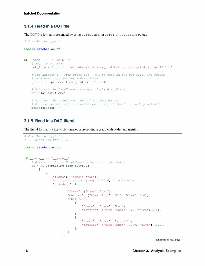
3.1.5 Read in a DAG literal

The literal format is a list of dictionaries representing a graph with nodes and metrics.

#!/usr/bin/env python# -*- encoding: utf-8 -*-


if __name__ == "__main__":# Define a literal GraphFrame using a list of dicts.gf = ht.GraphFrame.from_literal(

[{

"frame": {"name": "foo"},"metrics": {"time (inc)": 130.0, "time": 0.0},"children": [

{"frame": {"name": "bar"},"metrics": {"time (inc)": 20.0, "time": 5.0},"children": [

{"frame": {"name": "baz"},"metrics": {"time (inc)": 5.0, "time": 5.0},

},{

"frame": {"name": "grault"},"metrics": {"time (inc)": 10.0, "time": 10.0},

},],

},






{"frame": {"name": "qux"},"metrics": {"time (inc)": 60.0, "time": 0.0},"children": [

{"frame": {"name": "quux"},"metrics": {"time (inc)": 60.0, "time": 5.0},"children": [

{"frame": {"name": "corge"},"metrics": {"time (inc)": 55.0, "time": 10.0},"children": [

{"frame": {"name": "bar"},"metrics": {

"time (inc)": 20.0,"time": 5.0,

},"children": [

{"frame": {"name": "baz"},"metrics": {

"time (inc)": 5.0,"time": 5.0,

},},{

"frame": {"name": "grault"},"metrics": {

"time (inc)": 10.0,"time": 10.0,

},},

],},{

"frame": {"name": "grault"},"metrics": {

"time (inc)": 10.0,"time": 10.0,

},},{

"frame": {"name": "garply"},"metrics": {

"time (inc)": 15.0,"time": 15.0,

},},

],}

],}

],},{

"frame": {"name": "waldo"},(continues on next page)

3.1. Reading different file formats 17



"metrics": {"time (inc)": 50.0, "time": 0.0},"children": [

{"frame": {"name": "fred"},"metrics": {"time (inc)": 35.0, "time": 5.0},"children": [

{"frame": {"name": "plugh"},"metrics": {"time (inc)": 5.0, "time": 5.0},

},{

"frame": {"name": "xyzzy"},"metrics": {"time (inc)": 25.0, "time": 5.0},"children": [

{"frame": {"name": "thud"},"metrics": {

"time (inc)": 25.0,"time": 5.0,

},"children": [

{"frame": {"name": "baz"},"metrics": {

"time (inc)": 5.0,"time": 5.0,

},},{

"frame": {"name": "garply"},"metrics": {

"time (inc)": 15.0,"time": 15.0,

},},

],}

],},

],},{

"frame": {"name": "garply"},"metrics": {"time (inc)": 15.0, "time": 15.0},

},],

},],

},{

"frame": {"name": " (hoge)"},"metrics": {"time (inc)": 30.0, "time": 0.0},"children": [

{"frame": {"name": "( (piyo)"},"metrics": {"time (inc)": 15.0, "time": 5.0},"children": [





{"frame": {"name": " (fuga)"},"metrics": {"time (inc)": 5.0, "time": 5.0},

},{

"frame": {"name": " (hogera)"},"metrics": {"time (inc)": 5.0, "time": 5.0},

},],

},{

"frame": {"name": " (hogehoge)"},"metrics": {"time (inc)": 15.0, "time": 15.0},

},],

},]

)



3.2 Basic Examples

3.2.1 Applying scalar operations to attributes

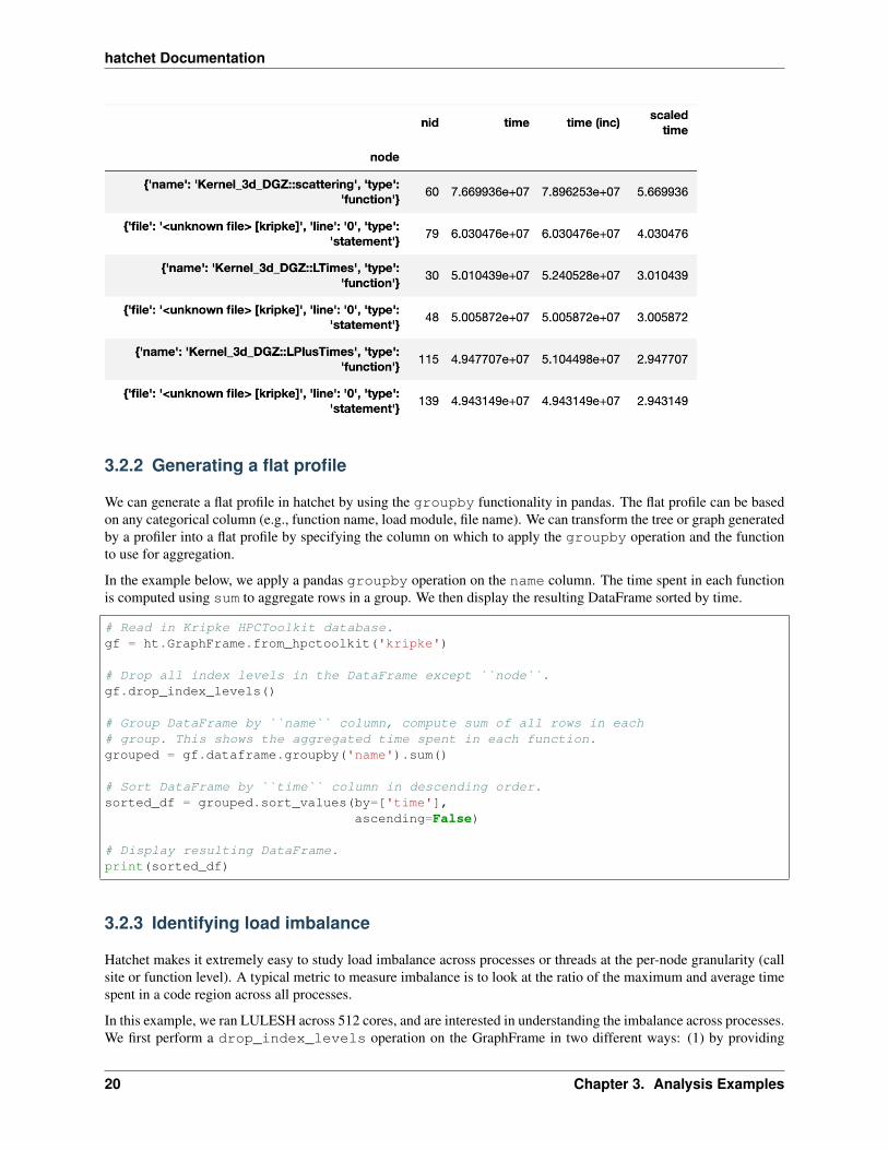
Individual numeric columns in the dataframe can be scaled or offset by a constant using the native pandas operations.We make a copy of the original graphframe, and modify the dataframe directly. In this example, we offset the timecolumn by -2 and scale it by 1/1e7, storing the result in a new column in the dataframe called scaled time.

gf = ht.GraphFrame.from_hpctoolkit('kripke')gf.drop_index_levels()

offset = 1e7gf.dataframe['scaled time'] = (gf.dataframe['time'] / offset) - 2sorted_df = gf.dataframe.sort_values(by=['scaled time'], ascending=False)print(sorted_df)

3.2. Basic Examples 19


3.2.2 Generating a flat profile

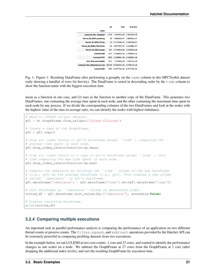
We can generate a flat profile in hatchet by using the groupby functionality in pandas. The flat profile can be basedon any categorical column (e.g., function name, load module, file name). We can transform the tree or graph generatedby a profiler into a flat profile by specifying the column on which to apply the groupby operation and the functionto use for aggregation.

In the example below, we apply a pandas groupby operation on the name column. The time spent in each functionis computed using sum to aggregate rows in a group. We then display the resulting DataFrame sorted by time.

# Read in Kripke HPCToolkit database.gf = ht.GraphFrame.from_hpctoolkit('kripke')

# Drop all index levels in the DataFrame except ``node``.gf.drop_index_levels()

# Group DataFrame by ``name`` column, compute sum of all rows in each# group. This shows the aggregated time spent in each function.grouped = gf.dataframe.groupby('name').sum()

# Sort DataFrame by ``time`` column in descending order.sorted_df = grouped.sort_values(by=['time'],

ascending=False)

# Display resulting DataFrame.print(sorted_df)

3.2.3 Identifying load imbalance

Hatchet makes it extremely easy to study load imbalance across processes or threads at the per-node granularity (callsite or function level). A typical metric to measure imbalance is to look at the ratio of the maximum and average timespent in a code region across all processes.

In this example, we ran LULESH across 512 cores, and are interested in understanding the imbalance across processes.We first perform a drop_index_levels operation on the GraphFrame in two different ways: (1) by providing



Fig. 1: Figure 1: Resulting DataFrame after performing a groupby on the name column in this HPCToolkit dataset(only showing a handful of rows for brevity). The DataFrame is sorted in descending order by the time column toshow the function name with the biggest execution time.

mean as a function in one case, and (2) max as the function to another copy of the DataFrame. This generates twoDataFrames, one containing the average time spent in each node, and the other containing the maximum time spent ineach node by any process. If we divide the corresponding columns of the two DataFrames and look at the nodes withthe highest value of the max-to-average ratio, we can identify the nodes with highest imbalance.

# Read in LULESH Caliper dataset.gf1 = ht.GraphFrame.from_caliper('lulesh-512cores')

# Create a copy of the GraphFrame.gf2 = gf1.copy()

# Drop all index levels in gf1's DataFrame except ``node``, computing the# average time spent in each node.gf1.drop_index_levels(function=np.mean)

# Drop all index levels in a copy of gf1's DataFrame except ``node``, this# time computing the max time spent in each node.gf2.drop_index_levels(function=np.max)

# Compute the imbalance by dividing the ``time`` column in the max DataFrame# (i.e., gf2) by the average DataFrame (i.e., gf1). This creates a new column# called ``imbalance`` in gf1's DataFrame.gf1.dataframe['imbalance'] = gf2.dataframe['time'].div(gf1.dataframe['time'])

# Sort DataFrame by ``imbalance`` column in descending order.sorted_df = gf1.dataframe.sort_values(by=['imbalance'], ascending=False)


3.2.4 Comparing multiple executions

An important task in parallel performance analysis is comparing the performance of an application on two differentthread counts or process counts. The filter, squash, and subtract operations provided by the Hatchet API canbe extremely powerful in comparing profiling datasets from two executions.

In the example below, we ran LULESH at two core counts: 1 core and 27 cores, and wanted to identify the performancechanges as one scales on a node. We subtract the GraphFrame at 27 cores from the GraphFrame at 1 core (afterdropping the additional index levels), and sort the resulting GraphFrame by execution time.

3.2. Basic Examples 21


Fig. 2: Figure 2: Resulting DataFrame showing the imbalance in this Caliper dataset (only showing a handful ofrows for brevity). The DataFrame is sorted in descending order by the new imbalance column calculated bydividing the max/average time of each function. The function with the highest level of imbalance within a node isLagrangeNodal with an imbalance of 2.49.

# Read in LULESH Caliper dataset at 1 core.gf1 = ht.GraphFrame.from_caliper('lulesh-1core.json')

# Read in LULESH Caliper dataset at 27 cores.gf2 = ht.GraphFrame.from_caliper('lulesh-27cores.json')

# Drop all index levels in gf2's DataFrame except ``node``.gf2.drop_index_levels()

# Subtract the GraphFrame at 27 cores from the GraphFrame at 1 core, and# store result in a new GraphFrame.gf3 = gf2 - gf1

# Sort resulting DataFrame by ``time`` column in descending order.sorted_df = gf3.dataframe.sort_values(by=['time'], ascending=False)


Fig. 3: Figure 3: Resulting DataFrame showing the performance differences when running LULESH at 1 core vs. 27cores (only showing a handful of rows for brevity). The DataFrame sorts the function names in descending order bythe time column. The TimeIncrement has the largest difference in execution time of 8.5e6 as the code scalesfrom 1 to 27 cores.

3.2.5 Filtering by library

Sometimes, users are interested in analyzing how a particular library, such as PetSc or MPI, is used by their applicationand how the time spent in the library changes as we scale to a larger number of processes.

In this next example, we compare two datasets generated from executions at different numbers of MPI processes.We read in two datasets of LULESH at 27 and 512 MPI processes, respectively, and filter them both on the namecolumn by matching the names against ^MPI. After the filtering operation, we squash the DataFrames to generate



GraphFrames that just contain the MPI calls from the original datasets. We can now subtract the squashed datasets toidentify the biggest offenders.

# Read in LULESH Caliper dataset at 27 cores.gf1 = GraphFrame.from_caliper('lulesh-27cores')

# Drop all index levels in DataFrame except ``node``.gf1.drop_index_levels()

# Filter GraphFrame by names that start with ``MPI``. This only filters the ## DataFrame. The Graph and DataFrame are now out of sync.filtered_gf1 = gf1.filter(lambda x: x['name'].startswith('MPI'))

# Squash GraphFrame, the nodes in the Graph now match what's in the# DataFrame.squashed_gf1 = filtered_gf1.squash()

# Read in LULESH Caliper dataset at 512 cores, drop all index levels except# ``node``, filter and squash the GraphFrame, leaving only nodes that start# with ``MPI``.gf2 = GraphFrame.from_caliper('lulesh-512cores')gf2.drop_index_levels()filtered_gf2 = gf2.filter(lambda x: x['name'].startswith('MPI'))squashed_gf2 = filtered_gf2.squash()

# Subtract the two GraphFrames, store the result in a new GraphFrame.diff_gf = squashed_gf2 - squashed_gf1

# Sort resulting DataFrame by ``time`` column in descending order.sorted_df = diff_gf.dataframe.sort_values(by=['time'], ascending=False)


Fig. 4: Figure 4: Resulting DataFrame showing the MPI performance differences when running LULESH at 27 coresvs. 512 cores. The DataFrame sorts the MPI functions in descending order by the time column. In this example, theMPI_Allreduce function sees the largest increase in time scaling from 27 to 512 cores.

3.3 Scaling Performance Examples

3.3.1 Analyzing strong scaling performance

Hatchet can be used for a strong scaling analysis of applications. In this example, we compare the performance ofLULESH running on 1 and 64 cores. By executing a simple divide of the two datasets in Hatchet, we can quickly

3.3. Scaling Performance Examples 23


pinpoint bottleneck functions. In the resulting graph, we invert the color scheme, so that functions that did not scalewell (i.e., have a low speedup) are colored in red.

gf_1core = ht.GraphFrame.from_caliper('lulesh*-1core.json')gf_64cores = ht.GraphFrame.from_caliper('lulesh*-64cores.json')

gf_64cores["time"] *= 64

gf_strong_scale = gf_1core / gf_64cores

/ =

3.3.2 Analyzing weak scaling performance

Hatchet can be used for comparing parallel scaling performance of applications. In this example, we compare theperformance of LULESH running on 1 and 27 cores. By executing a simple divide of the two datasets in Hatchet,we can quickly identify which function calls did or did not scale well. In the resulting graph, we invert the colorscheme, so that functions that did not scale well (i.e., have a low speedup) are colored in red.

gf_1core = ht.GraphFrame.from_caliper('lulesh*-1core.json')gf_27cores = ht.GraphFrame.from_caliper('lulesh*-27cores.json')

gf_weak_scale = gf_1core / gf_27cores



/ =

3.3.3 Identifying scaling bottlenecks

Hatchet can also be used to analyze data in a weak or strong scaling performance study. In this example, we ranLULESH from 1 to 512 cores on third powers of some numbers. We read in all the datasets into Hatchet, and foreach dataset, we use a few lines of code to filter the regions where the code spends most of the time. We then use thepandas’ pivot and plot operations to generate a stacked bar chart that shows how the time spent in different regions ofLULESH changes as the code scales.

# Grab all LULESH Caliper datasets, store in a sorted list.datasets = glob.glob('lulesh*.json')datasets.sort()

# For each dataset, create a new GraphFrame, and drop all index levels,# except ``node``. Insert filtered graphframe into a list.dataframes = []for dataset in datasets:

gf = ht.GraphFrame.from_caliper(dataset)gf.drop_index_levels()

# Grab the number of processes from the file name, store this as a new# column in the DataFrame.num_pes = re.match('(.*)-(\d+)(.*)', dataset).group(2)gf.dataframe['pes'] = num_pes

# Filter the GraphFrame keeping only those rows with ``time`` greater# than 1e6.filtered_gf = gf.filter(lambda x: x['time'] > 1e6)

# Insert the filtered GraphFrame into a list.





dataframes.append(filtered_gf.dataframe)

# Concatenate all DataFrames into a single DataFrame called ``result``.result = pd.concat(dataframes)

# Reshape the Dataframe, such that ``pes`` is an index column, ``name``# fields are the new column names, and the values for each cell is the# ``time`` fields.pivot_df = result.pivot(index='pes', columns='name', values='time')

# Make a stacked bar chart using the data in the pivot table above.pivot_df.loc[:,:].plot.bar(stacked=True, figsize=(10,7))

Fig. 5: Figure 5: Resulting stacked bar chart showing the time spent in different functions in LULESH as the codescales from 1 up to 512 processes. In this example, the CalcHourglassControlForElems function increasesin runtime moving from 1 to 8 processes, then stays constant.

We use the same LULESH scaling datasets above to filter for time-consuming functions that start with the stringCalc. This data is used to produce a line chart showing the performance of each function as the number of processesis increased. One of the functions (CalcMonotonicQRegionForElems) does not occur until the number ofprocesses is greater than 1.

datasets = glob.glob('lulesh*.json')datasets.sort()

dataframes = []for dataset in datasets:

gf = ht.GraphFrame.from_caliper(dataset)gf.drop_index_levels()

num_pes = re.match('(.*)-(\d+)(.*)', dataset).group(2)gf.dataframe['pes'] = num_pesfiltered_gf = gf.filter(lambda x: x["time"] > 1e6 and x["name"].startswith('Calc

→˓'))





dataframes.append(filtered_gf.dataframe)

result = pd.concat(dataframes)pivot_df = result.pivot(index='pes', columns='name', values='time')pivot_df.loc[:,:].plot.line(figsize=(10, 7))

If you encounter bugs while using hatchet, you can report them by opening an issue on GitHub.

If you are referencing hatchet in a publication, please cite the following paper:

• Abhinav Bhatele, Stephanie Brink, and Todd Gamblin. Hatchet: Pruning the Overgrowth in Parallel Profiles.In Proceedings of the International Conference for High Performance Computing, Networking, Storage andAnalysis (SC ‘19). ACM, New York, NY, USA. DOI


http://github.com/llnl/hatchet/issues

http://www.cs.umd.edu/~bhatele/pubs/pdf/2019/sc2019.pdf

https://doi.org/10.1145/3295500.3356219

CHAPTER 4

Basic Tutorial: Hatchet 101

This tutorial introduces how to use hatchet, including basics about:

• Installing hatchet

• Using the pandas API

• Using the hatchet API

4.1 Installing Hatchet and Tutorial Setup

You can install hatchet using pip:


After installing hatchet, you can import hatchet when running the Python interpreter in interactive mode:

$ pythonPython 3.7.7 (default, Mar 14 2020, 02:39:01)[Clang 10.0.1 (clang-1001.0.46.4)] on darwinType "help", "copyright", "credits" or "license" for more information.>>>

Typing import hatchet at the prompt should succeed without any error messages:

>>> import hatchet as ht>>>

You are good to go!

The Hatchet repository includes stand-alone Python-based Jupyter notebook examples based on this tutorial. You canfind them in the hatchet GitHub repository. You can get a local copy of the repository using git:


29

https://github.com/LLNL/hatchet/tree/develop/docs/examples


You will find the tutorial notebooks in your local hatchet repository under docs/examples/tutorial/.

4.2 Introduction

You can read in a dataset into Hatchet for analysis by using one of several from_ static methods. For example, youcan read in a Caliper JSON file as follows:

>>> import hatchet as ht>>> caliper_file = 'lulesh-annotation-profile-1core.json'>>> gf = ht.GraphFrame.from_caliper_json(caliper_file)>>>

At this point, your input file (profile) has been loaded into Hatchet’s data structure, known as a GraphFrame. Hatchet’sGraphFrame contains a pandas DataFrame and a corresponding graph.

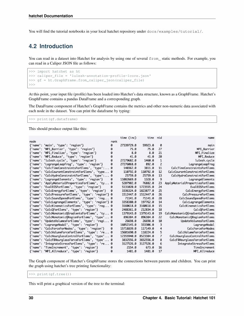
The DataFrame component of Hatchet’s GraphFrame contains the metrics and other non-numeric data associated witheach node in the dataset. You can print the dataframe by typing:

>>> print(gf.dataframe)

This should produce output like this:

The Graph component of Hatchet’s GraphFrame stores the connections between parents and children. You can printthe graph using hatchet’s tree printing functionality:

>>> print(gf.tree())

This will print a graphical version of the tree to the terminal:

30 Chapter 4. Basic Tutorial: Hatchet 101


4.3 Analyzing the DataFrame using pandas

The DataFrame is one of two components that makeup the GraphFrame in hatchet. The pandas DataFramestores the performance metrics and other non-numeric data for all nodes in the graph.

You can apply any pandas operations to the dataframe in hatchet. Note that modifying the dataframe in hatchet outsideof the hatchet API is not recommended because operations that modify the dataframe can make the dataframe andgraph inconsistent.

By default, the rows in the dataframe are sorted in traversal order. Sorting the rows by a different column can be doneas follows:

>>> sorted_df = gf.dataframe.sort_values(by=['time'], ascending=False)

Individual numeric columns in the dataframe can be scaled or offset by a constant using native pandas operations. Inthe following example, we add a new column called scale to the existing dataframe, and print the dataframe sortedby this new column from lowest to highest:

>>> gf.dataframe['scale'] = gf.dataframe['time'] * 4>>> sorted_df = gf.dataframe.sort_values(by=['scale'], ascending=True)

4.4 Analyzing the Graph via printing

Hatchet provides several methods of visualizing graphs. In this section, we show how a user can use the tree()method to convert the graph to a string that can be displayed to standard output. This function has several differentparameters that can alter the output. To look at all the available parameters, you can look at the docstrings as follows:

4.3. Analyzing the DataFrame using pandas 31


>>> help(gf.tree)

Help on method tree in module hatchet.graphframe:

tree(metric_column='time', precision=3, name_column='name', expand_name=False,context_column='file', rank=0, thread=0, depth=10000, highlight_name=False,invert_colormap=False) method of hatchet.graphframe.GraphFrame instance

Format this graphframe as a tree and return the resulting string.

To print the graph output:

>>> gf.tree()

By default, the graph printout displays next to each node values in the time column of the dataframe. To displayanother column, change the argument to the metric_column= parameter:

>>> gf.tree(metric_column='time (inc)')

To view a subset of the nodes in the graph, a user can change the depth= value to indicate how many levels of thetree to display. By default, all levels in the tree are displayed. In the following example, we only ask to display thefirst three levels of the tree, where the root is the first level:

>>> gf.tree(depth=3)

By default, the tree() method uses a red-green colormap, whereby nodes with high metric values are colored red,while nodes with low metric values are colored green. In some use cases, a user may want to reverse the colormap todraw attention to certain nodes, such as performing a division of two graphframes to compute speedup:

4.4. Analyzing the Graph via printing 33


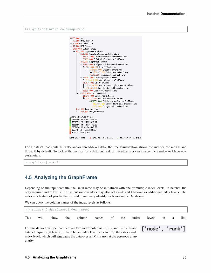
>>> gf.tree(invert_colormap=True)

For a dataset that contains rank- and/or thread-level data, the tree visualization shows the metrics for rank 0 andthread 0 by default. To look at the metrics for a different rank or thread, a user can change the rank= or thread=parameters:

>>> gf.tree(rank=4)

4.5 Analyzing the GraphFrame

Depending on the input data file, the DataFrame may be initialized with one or multiple index levels. In hatchet, theonly required index level is node, but some readers may also set rank and thread as additional index levels. Theindex is a feature of pandas that is used to uniquely identify each row in the Dataframe.

We can query the column names of the index levels as follows:

>>> print(gf.dataframe.index.names)

This will show the column names of the index levels in a list:

For this dataset, we see that there are two index columns: node and rank. Sincehatchet requires (at least) node to be an index level, we can drop the extra rankindex level, which will aggregate the data over all MPI ranks at the per-node gran-ularity.

4.5. Analyzing the GraphFrame 35


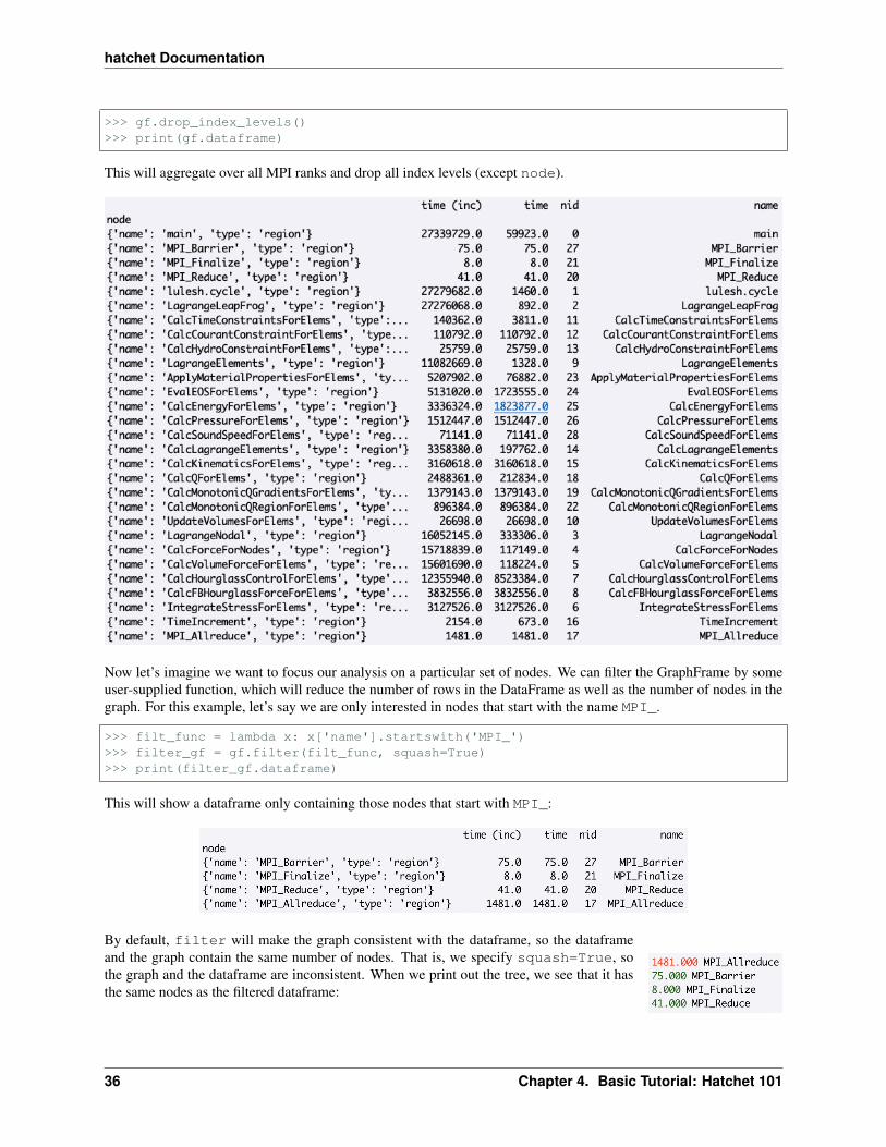
>>> gf.drop_index_levels()>>> print(gf.dataframe)

This will aggregate over all MPI ranks and drop all index levels (except node).

Now let’s imagine we want to focus our analysis on a particular set of nodes. We can filter the GraphFrame by someuser-supplied function, which will reduce the number of rows in the DataFrame as well as the number of nodes in thegraph. For this example, let’s say we are only interested in nodes that start with the name MPI_.

>>> filt_func = lambda x: x['name'].startswith('MPI_')>>> filter_gf = gf.filter(filt_func, squash=True)>>> print(filter_gf.dataframe)

This will show a dataframe only containing those nodes that start with MPI_:

By default, filter will make the graph consistent with the dataframe, so the dataframeand the graph contain the same number of nodes. That is, we specify squash=True, sothe graph and the dataframe are inconsistent. When we print out the tree, we see that it hasthe same nodes as the filtered dataframe:



4.6 Analyzing Multiple GraphFrames

With hatchet, we can perform mathematical operators on multiple GraphFrames. This isuseful for comparing the performance of functions at increasing concurrency or computing speedup of two differentimplementations of the same function, for example.

In the example below, we have two LULESH profiles collected at 1 and 64 cores using Caliper. The graphs of these twoprofiles are slightly different in structure. Due to the scale of the 64 core LULESH run, its profile contains additionalMPI-related functions than the 1 core run. With hatchet, we can operate on profiles with different graph structures byfirst unifying the graphs, and the resulting graph annotates the nodes to indicate which graph the node originated from.

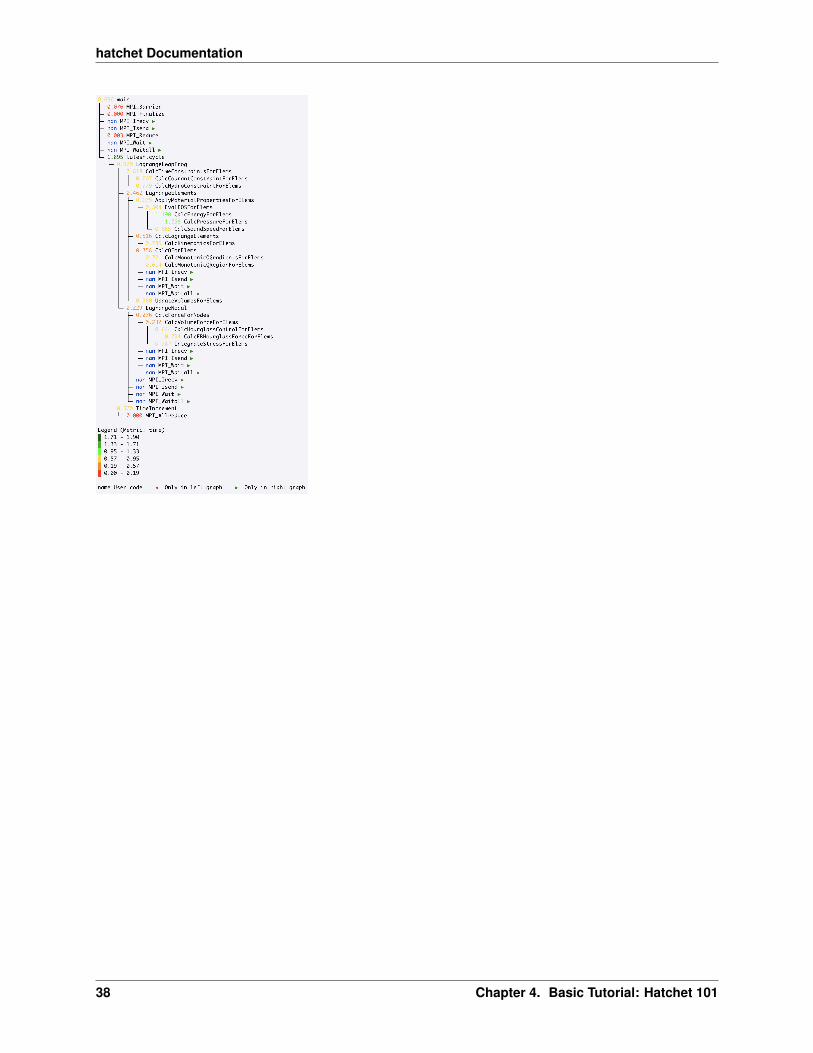
By dividing the profiles, we can analyze how the functions scale at higher concurrencies. Before performing thedivision operator, we drop the extra rank index level in both profiles, which aggregates the data over all MPI ranksat the per-node granularity. When printing the tree, we specify invert_colormap=True, so that nodes with goodspeedup (i.e., low values) are colored green, while nodes with poor speedup (i.e., high values) are colored red. Bydefault, nodes with low values are colored green, while high values are colored red.

Additionally, because the 64 core profile contained more nodes than the 1 core profile, the resulting tree is annotatedwith green triangles pointing to the right, indicating that these nodes originally came from the right tree (when thinkingof gf3 = gf/gf2). In hatchet, those nodes contained in only one of the two trees are initialized with a value of nan, andare colored in blue.

>>> caliper_file_1core = 'lulesh-annotation-profile-1core.json'>>> caliper_file_64cores = 'lulesh-annotation-profile-64cores.json'>>> gf = ht.GraphFrame.from_caliper_json(caliper_file_1core)>>> gf2 = ht.GraphFrame.from_caliper_json(caliper_file_64cores)>>> gf.drop_index_levels()>>> gf2.drop_index_levels()>>> gf3 = gf/gf2>>> gf3.tree(invert_colormap=True)

/ =

4.6. Analyzing Multiple GraphFrames 37

CHAPTER 5

Publications and Presentations

5.1 Publications

• Stephanie Brink, Ian Lumsden, Connor Scully-Allison, Katy Williams, Olga Pearce, Todd Gamblin, MichelaTaufer, Katherine Isaacs, Abhinav Bhatele. Usability and Performance Improvements in Hatchet. Presentedat the ProTools 2020 Workshop, held in conjunction with the International Conference for High PerformanceComputing, Networking, Storage and Analysis (SC ‘20), held virtually.

• Abhinav Bhatele, Stephanie Brink, and Todd Gamblin. Hatchet: Pruning the Overgrowth in Parallel Profiles.In Proceedings of the International Conference for High Performance Computing, Networking, Storage andAnalysis (SC ‘19), Denver, CO.

5.2 Posters

• Ian Lumsden. Graph-Based Profiling Analysis using Hatchet. Presented at SC ‘20. Slides | Video Presentation

• Suraj P. Kesavan, Harsh Bhatia, Abhinav Bhatele, Stephanie Brink, Olga Pearce, Todd Gamblin, Peer-TimoBremer, and Kwan-Liu Ma. Scalable Comparative Visualization of Ensembles of Call Graphs Using CallFlow.Presented at SC ‘20.

5.3 Tutorials

• Performance Analysis using Hatchet, LLNL, July 29/31, 2020.

39

https://pssg.cs.umd.edu/assets/papers/2020-11-hatchet-protools.pdf

https://protools20.github.io/

https://doi.org/10.1145/3295500.3356219

https://globalcomputing.group/assets/img/sc20/posters/ian.pdf

https://globalcomputing.group/assets/img/sc20/bestposters/ian.pdf

https://www.youtube.com/watch?v=j-FRGnLBo4U&feature=youtu.be


40 Chapter 5. Publications and Presentations

CHAPTER 6

hatchet package

6.1 Subpackages

6.1.1 hatchet.cython_modules package

Subpackages

hatchet.cython_modules.libs package

Submodules

hatchet.cython_modules.libs.subtract_metrics module

Module contents

Submodules

hatchet.cython_modules.subtract_metrics module

Module contents

6.1.2 hatchet.external package

Submodules

hatchet.external.console module

class hatchet.external.console.ConsoleRenderer(unicode=False, color=False)Bases: object

41


colors_disabled = <hatchet.external.console.ConsoleRenderer.colors_disabled object>

class colors_enabledBases: object

bg_white_255 = '\x1b[48;5;246m'

blue = '\x1b[34m'

colormap = ['\x1b[38;5;196m', '\x1b[38;5;208m', '\x1b[38;5;220m', '\x1b[38;5;46m', '\x1b[38;5;34m', '\x1b[38;5;22m']

cyan = '\x1b[36m'

dark_gray_255 = '\x1b[38;5;232m'

end = '\x1b[0m'

faint = '\x1b[2m'

left = '\x1b[38;5;160m'

right = '\x1b[38;5;28m'

render(roots, dataframe, **kwargs)

render_frame(node, dataframe, indent=”, child_indent=”)

render_legend()

render_preamble()

Module contents

6.1.3 hatchet.readers package

Submodules

hatchet.readers.caliper_reader module

class hatchet.readers.caliper_reader.CaliperReader(filename_or_stream, query=”)Bases: object

Read in a Caliper file (cali or split JSON) or file-like object.

create_graph()

read()Read the caliper JSON file to extract the calling context tree.

read_json_sections()

hatchet.readers.gprof_dot_reader module

class hatchet.readers.gprof_dot_reader.GprofDotReader(filename)Bases: object

Read in gprof/callgrind output in dot format generated by gprof2dot.

create_graph()Read the DOT files to create a graph.

read()Read the DOT file generated by gprof2dot to create a graphframe. The DOT file contains a call graph.

42 Chapter 6. hatchet package


hatchet.readers.hpctoolkit_reader module

class hatchet.readers.hpctoolkit_reader.HPCToolkitReader(dir_name)Bases: object

Read in the various sections of an HPCToolkit experiment.xml file and metric-db files.

create_node_dict(nid, hnode, name, node_type, src_file, line, module)Create a dict with all the node attributes.

fill_tables()Read certain sections of the experiment.xml file to create dicts of load modules, src_files, proce-dure_names, and metric_names.

parse_xml_children(xml_node, hnode)Parses all children of an XML node.

parse_xml_node(xml_node, parent_nid, parent_line, hparent)Parses an XML node and its children recursively.

read()Read the experiment.xml file to extract the calling context tree and create a dataframe out of it. Then mergethe two dataframes to create the final dataframe.

Returns new GraphFrame with HPCToolkit data.

Return type (GraphFrame)

read_all_metricdb_files()Read all the metric-db files and create a dataframe with num_nodes X num_metricdb_files rows andnum_metrics columns. Three additional columns store the node id, MPI process rank, and thread id (ifapplicable).

hatchet.readers.hpctoolkit_reader.init_shared_array(buf_)Initialize shared array.

hatchet.readers.hpctoolkit_reader.read_metricdb_file(args)Read a single metricdb file into a 1D array.

Module contents

6.1.4 hatchet.util package

Submodules

hatchet.util.config module

hatchet.util.deprecated module

hatchet.util.deprecated.deprecated_params(**old_to_new)

hatchet.util.deprecated.rename_kwargs(fname, old_to_new, kwargs)

hatchet.util.dot module

hatchet.util.dot.to_dot(hnode, dataframe, metric, name, rank, thread, threshold, visited)Write to graphviz dot format.

6.1. Subpackages 43


hatchet.util.dot.trees_to_dot(roots, dataframe, metric, name, rank, thread, threshold)Calls to_dot in turn for each tree in the graph/forest.

hatchet.util.executable module

hatchet.util.executable.which(executable)Finds an executable in the user’s PATH like command-line which.

Parameters executable (str) – executable to search for

hatchet.util.profiler module

class hatchet.util.profiler.ProfilerBases: object

Wrapper class around cProfile. Exports a pstats file to be read by the pstats reader.

reset()Description: Resets the profilier.

start()Description: Place before the block of code to be profiled.

stop()Description: Place at the end of the block of code being profiled.

write_to_file(filename=”, add_pstats_files=[])Description: Write the pstats object to a binary file to be read in by an appropriate source.

hatchet.util.profiler.print_incomptable_msg(stats_file)Function which makes the syntax cleaner in Profiler.write_to_file().

hatchet.util.timer module

class hatchet.util.timer.TimerBases: object

Simple phase timer with a context manager.

end_phase()

phase(name)

start_phase(phase)

Module contents

6.2 Submodules

6.3 hatchet.frame module

class hatchet.frame.Frame(attrs=None, **kwargs)Bases: object

The frame index for a node. The node only stores its frame.



Parameters attrs (dict) – dictionary of attributes and values

copy()

get(name, default=None)

tuple_reprMake a tuple of attributes and values based on reader.

values(names)Return a tuple of attribute values from this Frame.

6.4 hatchet.graph module

class hatchet.graph.Graph(roots)Bases: object

A possibly multi-rooted tree or graph from one input dataset.

copy(old_to_new=None)Create and return a copy of this graph.

Parameters old_to_new (dict, optional) – if provided, this dictionary will be popu-lated with mappings from old node -> new node

enumerate_depth()

enumerate_traverse()

find_merges()Find nodes that have the same parent and frame.

Find nodes that have the same parent and duplicate frame, and return a mapping from nodes that shouldbe eliminated to nodes they should be merged into.

Returns dictionary from nodes to their merge targets

Return type (dict)

static from_lists(*roots)Convenience method to invoke Node.from_lists() on each root value.

is_tree()True if this graph is a tree, false otherwise.

merge_nodes(merges)Merge some nodes in a graph into others.

merges is a dictionary keyed by old nodes, with values equal to the nodes that they need to be mergedinto. Old nodes’ parents and children are connected to the new node.

Parameters merges (dict) – dictionary from source nodes -> targets

normalize()

traverse(order=’pre’, attrs=None, visited=None)Preorder traversal of all roots of this Graph.

Parameters attrs (list or str, optional) – If provided, extract these fields fromnodes while traversing and yield them. See traverse() for details.

Only preorder traversal is currently supported.

6.4. hatchet.graph module 45


union(other, old_to_new=None)Create the union of self and other and return it as a new Graph.

This creates a new graph and does not modify self or other. The new Graph has entirely new nodes.

Parameters

• other (Graph) – another Graph

• old_to_new (dict, optional) – if provided, this dictionary will be populated withmappings from old node -> new node

Returns new Graph containing all nodes and edges from self and other

Return type (Graph)

hatchet.graph.index_by(attr, objects)Put objects into lists based on the value of an attribute.

Returns dictionary of lists of objects, keyed by attribute value

Return type (dict)

6.5 hatchet.graphframe module

exception hatchet.graphframe.EmptyFilterBases: Exception

Raised when a filter would otherwise return an empty GraphFrame.

class hatchet.graphframe.GraphFrame(graph, dataframe, exc_metrics=None,inc_metrics=None)

Bases: object

An input dataset is read into an object of this type, which includes a graph and a dataframe.

add(other, *args, **kwargs)Returns the column-wise sum of two graphframes as a new graphframe.

This graphframe is the union of self’s and other’s graphs, and does not modify self or other.

Returns new graphframe


copy()Return a shallow copy of the graphframe.

This copies the DataFrame, but the Graph is shared between self and the new GraphFrame.

deepcopy()Return a copy of the graphframe.

div(other, *args, **kwargs)Returns the column-wise float division of two graphframes as a new graphframe.




drop_index_levels(function=<function mean>)Drop all index levels but node.



filter(filter_obj, squash=True)Filter the dataframe using a user-supplied function.

Parameters

• filter_obj (callable, list, or QueryMatcher) – the filter to apply to theGraphFrame.

• squash (boolean, optional) – if True, automatically call squash for the user.

static from_caliper(filename, query)Read in a Caliper cali file.

Parameters

• filename (str) – name of a Caliper output file in .cali format

• query (str) – cali-query in CalQL format

static from_caliper_json(filename_or_stream)Read in a Caliper cali-query JSON-split file or an open file object.

Parameters filename_or_stream (str or file-like) – name of a Caliper JSON-split output file, or an open file object to read one

static from_cprofile(filename)Read in a pstats/prof file generated using python’s cProfile.

static from_gprof_dot(filename)Read in a DOT file generated by gprof2dot.

static from_hpctoolkit(dirname)Read an HPCToolkit database directory into a new GraphFrame.

Parameters dirname (str) – parent directory of an HPCToolkit experiment.xml file

Returns new GraphFrame containing HPCToolkit profile data


static from_lists(*lists)Make a simple GraphFrame from lists.

This creates a Graph from lists (see Graph.from_lists()) and uses it as the index for a new Graph-Frame. Every node in the new graph has exclusive time of 1 and inclusive time is computed automatically.

static from_literal(graph_dict)Create a GraphFrame from a list of dictionaries.

static from_pyinstrument(filename)Read in a JSON file generated using Pyinstrument.

groupby_aggregate(groupby_function, agg_function)Groupby-aggregate dataframe and reindex the Graph.

Reindex the graph to match the groupby-aggregated dataframe.

Update the frame attributes to contain those columns in the dataframe index.

Parameters

• self (graphframe) – self’s graphframe

• groupby_function – groupby function on dataframe

• agg_function – aggregate function on dataframe

6.5. hatchet.graphframe module 47


Returns new graphframe with reindexed graph and groupby-aggregated dataframe


mul(other, *args, **kwargs)Returns the column-wise float multiplication of two graphframes as a new graphframe.




squash()Rewrite the Graph to include only nodes present in the DataFrame’s rows.

This can be used to simplify the Graph, or to normalize Graph indexes between two GraphFrames.

sub(other, *args, **kwargs)Returns the column-wise difference of two graphframes as a new graphframe.




subgraph_sum(columns, out_columns=None, function=<function GraphFrame.<lambda>>)Compute sum of elements in subgraphs.

For each row in the graph, out_columns will contain the element-wise sum of all values in columnsfor that row’s node and all of its descendants.

This algorithm is worst-case quadratic in the size of the graph, so we try to call subtree_sum if we can.In general, there is not a particularly efficient algorithm known for subgraph sums, so this does about aswell as we know how.

Parameters

• columns (list of str) – names of columns to sum (default: all columns)

• out_columns (list of str) – names of columns to store results (default: in place)

• function (callable) – associative operator used to sum elements, sum of an all-NAseries is NaN (default: sum(min_count=1))

subtree_sum(columns, out_columns=None, function=<function GraphFrame.<lambda>>)Compute sum of elements in subtrees. Valid only for trees.

For each row in the graph, out_columns will contain the element-wise sum of all values in columnsfor that row’s node and all of its descendants.

This algorithm will multiply count nodes with in-degree higher than one – i.e., it is only correct for trees.Prefer using subgraph_sum (which calls subtree_sum if it can), unless you have a good reason notto.

Parameters

• columns (list of str) – names of columns to sum (default: all columns)

• out_columns (list of str) – names of columns to store results (default: in place)

• function (callable) – associative operator used to sum elements, sum of an all-NAseries is NaN (default: sum(min_count=1))

to_dot(metric=’time’, name=’name’, rank=0, thread=0, threshold=0.0)Write the graph in the graphviz dot format: https://www.graphviz.org/doc/info/lang.html




to_flamegraph(metric=’time’, name=’name’, rank=0, thread=0, threshold=0.0)Write the graph in the folded stack output required by FlameGraph http://www.brendangregg.com/flamegraphs.html

to_literal(name=’name’, rank=0, thread=0)Format this graph as a list of dictionaries for Roundtrip visualizations.

tree(metric_column=’time’, precision=3, name_column=’name’, expand_name=False, con-text_column=’file’, rank=0, thread=0, depth=10000, highlight_name=False, in-vert_colormap=False)

Format this graphframe as a tree and return the resulting string.

unify(other)Returns a unified graphframe.

Ensure self and other have the same graph and same node IDs. This may change the node IDs in thedataframe.

Update the graphs in the graphframe if they differ.

update_inclusive_columns()Update inclusive columns (typically after operations that rewire the graph.

exception hatchet.graphframe.InvalidFilterBases: Exception

Raised when an invalid argument is passed to the filter function.

6.6 hatchet.node module

exception hatchet.node.MultiplePathErrorBases: Exception

Raised when a node is asked for a single path but has multiple.

class hatchet.node.Node(frame_obj, parent=None, hnid=-1, depth=-1)Bases: object

A node in the graph. The node only stores its frame.

add_child(node)Adds a child to this node’s list of children.

add_parent(node)Adds a parent to this node’s list of parents.

copy()Copy this node without preserving parents or children.

dag_equal(other, vs=None, vo=None)Check if DAG rooted at self has the same structure as that rooted at other.

classmethod from_lists(lists)Construct a hierarchy of nodes from recursive lists.

For example, this will construct a simple tree:

Node.from_lists(["a",

["b", "d", "e"],["c", "f", "g"],


6.6. hatchet.node module 49

http://www.brendangregg.com/flamegraphs.html

http://www.brendangregg.com/flamegraphs.html



])

a/ \

b c/ | | \

d e f g

And this will construct a simple diamond DAG:

d = Node(Frame(name="d"))Node.from_lists(

["a",["b", d],["c", d]

])

a/ \

b c\ /d

In the above examples, the ‘a’ represents a Node with its frame == Frame(name=”a”).

path(attrs=None)Path to this node from root. Raises if there are multiple paths.

Parameters attrs (str or list, optional) – attribute(s) to extract from Frames

This is useful for trees (where each node only has one path), as it just gets the only element from self.paths. This will fail with a MultiplePathError if there is more than one path to this node.

paths(attrs=None)List of tuples, one for each path from this node to any root.

Parameters attrs (str or list, optional) – attribute(s) to extract from Frames

Paths are tuples of Frame objects, or, if attrs is provided, they are paths containing the requested attributes.

traverse(order=’pre’, attrs=None, visited=None)Traverse the tree depth-first and yield each node.

Parameters

• order (str) – “pre” or “post” for preorder or postorder (default: pre)

• attrs (list or str, optional) – if provided, extract these fields from nodeswhile traversing and yield them

• visited (dict, optional) – dictionary in which each visited node’s in-degree willbe stored

hatchet.node.traversal_order(node)Deterministic key function for sorting nodes in traversals.



6.7 hatchet.query_matcher module

exception hatchet.query_matcher.InvalidQueryFilterBases: Exception

Raised when a query filter does not have a valid syntax

exception hatchet.query_matcher.InvalidQueryPathBases: Exception

Raised when a query does not have the correct syntax

class hatchet.query_matcher.QueryMatcher(query=None)Bases: object

Process and apply queries to GraphFrames.

apply(gf)Apply the query to a GraphFrame.

Parameters gf (GraphFrame) – the GraphFrame on which to apply the query.

Returns A list of lists representing the set of paths that match this query.

Return type (list)

match(wildcard_spec=’.’, filter_func=<function QueryMatcher.<lambda>>)Start a query with a root node described by the arguments.

Parameters

• wildcard_spec (str, optional, ".", "*", or "+") – the wildcard statusof the node (follows standard Regex syntax)

• filter_func (callable, optional) – a callable accepting only a row from aPandas DataFrame that is used to filter this node in the query

Returns The instance of the class that called this function (enables fluent design).

Return type (QueryMatcher)

rel(wildcard_spec=’.’, filter_func=<function QueryMatcher.<lambda>>)Add another edge and node to the query.

Parameters

• wildcard_spec (str, optional, ".", "*", or "+") – the wildcard statusof the node (follows standard Regex syntax)

• filter_func (callable, optional) – a callable accepting only a row from aPandas DataFrame that is used to filter this node in the query

Returns The instance of the class that called this function (enables fluent design).

Return type (QueryMatcher)

6.8 Module contents

6.7. hatchet.query_matcher module 51

CHAPTER 7

Indices and tables

• genindex

• modindex

• search

53


54 Chapter 7. Indices and tables

Python Module Index

hhatchet, 51hatchet.cython_modules, 41hatchet.cython_modules.libs, 41hatchet.external, 42hatchet.external.console, 41hatchet.frame, 44hatchet.graph, 45hatchet.graphframe, 46hatchet.node, 49hatchet.query_matcher, 51hatchet.readers, 43hatchet.readers.caliper_reader, 42hatchet.readers.gprof_dot_reader, 42hatchet.readers.hpctoolkit_reader, 43hatchet.util, 44hatchet.util.config, 43hatchet.util.deprecated, 43hatchet.util.dot, 43hatchet.util.executable, 44hatchet.util.profiler, 44hatchet.util.timer, 44

55


56 Python Module Index

Index

Aadd() (hatchet.graphframe.GraphFrame method), 46add_child() (hatchet.node.Node method), 49add_parent() (hatchet.node.Node method), 49apply() (hatchet.query_matcher.QueryMatcher

method), 51

Bbg_white_255 (hatchet.external.console.ConsoleRenderer.colors_enabled

attribute), 42blue (hatchet.external.console.ConsoleRenderer.colors_enabled

attribute), 42

CCaliperReader (class in

hatchet.readers.caliper_reader), 42colormap (hatchet.external.console.ConsoleRenderer.colors_enabled

attribute), 42colors_disabled (hatchet.external.console.ConsoleRenderer

attribute), 41ConsoleRenderer (class in

hatchet.external.console), 41ConsoleRenderer.colors_enabled (class in

hatchet.external.console), 42copy() (hatchet.frame.Frame method), 45copy() (hatchet.graph.Graph method), 45copy() (hatchet.graphframe.GraphFrame method), 46copy() (hatchet.node.Node method), 49create_graph() (hatchet.readers.caliper_reader.CaliperReader

method), 42create_graph() (hatchet.readers.gprof_dot_reader.GprofDotReader

method), 42create_node_dict()

(hatchet.readers.hpctoolkit_reader.HPCToolkitReadermethod), 43

cyan (hatchet.external.console.ConsoleRenderer.colors_enabledattribute), 42

Ddag_equal() (hatchet.node.Node method), 49

dark_gray_255 (hatchet.external.console.ConsoleRenderer.colors_enabledattribute), 42

deepcopy() (hatchet.graphframe.GraphFramemethod), 46

deprecated_params() (in modulehatchet.util.deprecated), 43

div() (hatchet.graphframe.GraphFrame method), 46drop_index_levels()

(hatchet.graphframe.GraphFrame method), 46

EEmptyFilter, 46end (hatchet.external.console.ConsoleRenderer.colors_enabled

attribute), 42end_phase() (hatchet.util.timer.Timer method), 44enumerate_depth() (hatchet.graph.Graph method),

45enumerate_traverse() (hatchet.graph.Graph

method), 45

Ffaint (hatchet.external.console.ConsoleRenderer.colors_enabled

attribute), 42fill_tables() (hatchet.readers.hpctoolkit_reader.HPCToolkitReader

method), 43filter() (hatchet.graphframe.GraphFrame method),

46find_merges() (hatchet.graph.Graph method), 45Frame (class in hatchet.frame), 44from_caliper() (hatchet.graphframe.GraphFrame

static method), 47from_caliper_json()

(hatchet.graphframe.GraphFrame staticmethod), 47

from_cprofile() (hatchet.graphframe.GraphFramestatic method), 47

from_gprof_dot() (hatchet.graphframe.GraphFramestatic method), 47

from_hpctoolkit()(hatchet.graphframe.GraphFrame static

57


method), 47from_lists() (hatchet.graph.Graph static method),

45from_lists() (hatchet.graphframe.GraphFrame

static method), 47from_lists() (hatchet.node.Node class method), 49from_literal() (hatchet.graphframe.GraphFrame

static method), 47from_pyinstrument()

(hatchet.graphframe.GraphFrame staticmethod), 47

Gget() (hatchet.frame.Frame method), 45GprofDotReader (class in

hatchet.readers.gprof_dot_reader), 42Graph (class in hatchet.graph), 45GraphFrame (class in hatchet.graphframe), 46groupby_aggregate()


Hhatchet (module), 51hatchet.cython_modules (module), 41hatchet.cython_modules.libs (module), 41hatchet.external (module), 42hatchet.external.console (module), 41hatchet.frame (module), 44hatchet.graph (module), 45hatchet.graphframe (module), 46hatchet.node (module), 49hatchet.query_matcher (module), 51hatchet.readers (module), 43hatchet.readers.caliper_reader (module),

42hatchet.readers.gprof_dot_reader (mod-

ule), 42hatchet.readers.hpctoolkit_reader (mod-

ule), 43hatchet.util (module), 44hatchet.util.config (module), 43hatchet.util.deprecated (module), 43hatchet.util.dot (module), 43hatchet.util.executable (module), 44hatchet.util.profiler (module), 44hatchet.util.timer (module), 44HPCToolkitReader (class in

hatchet.readers.hpctoolkit_reader), 43

Iindex_by() (in module hatchet.graph), 46init_shared_array() (in module

hatchet.readers.hpctoolkit_reader), 43InvalidFilter, 49

InvalidQueryFilter, 51InvalidQueryPath, 51is_tree() (hatchet.graph.Graph method), 45

Lleft (hatchet.external.console.ConsoleRenderer.colors_enabled

attribute), 42

Mmatch() (hatchet.query_matcher.QueryMatcher

method), 51merge_nodes() (hatchet.graph.Graph method), 45mul() (hatchet.graphframe.GraphFrame method), 48MultiplePathError, 49

NNode (class in hatchet.node), 49normalize() (hatchet.graph.Graph method), 45

Pparse_xml_children()


parse_xml_node() (hatchet.readers.hpctoolkit_reader.HPCToolkitReadermethod), 43

path() (hatchet.node.Node method), 50paths() (hatchet.node.Node method), 50phase() (hatchet.util.timer.Timer method), 44print_incomptable_msg() (in module

hatchet.util.profiler), 44Profiler (class in hatchet.util.profiler), 44

QQueryMatcher (class in hatchet.query_matcher), 51

Rread() (hatchet.readers.caliper_reader.CaliperReader

method), 42read() (hatchet.readers.gprof_dot_reader.GprofDotReader

method), 42read() (hatchet.readers.hpctoolkit_reader.HPCToolkitReader

method), 43read_all_metricdb_files()


read_json_sections()(hatchet.readers.caliper_reader.CaliperReadermethod), 42

read_metricdb_file() (in modulehatchet.readers.hpctoolkit_reader), 43

rel() (hatchet.query_matcher.QueryMatcher method),51

rename_kwargs() (in modulehatchet.util.deprecated), 43

58 Index


render() (hatchet.external.console.ConsoleRenderermethod), 42

render_frame() (hatchet.external.console.ConsoleRenderermethod), 42

render_legend() (hatchet.external.console.ConsoleRenderermethod), 42

render_preamble()(hatchet.external.console.ConsoleRenderermethod), 42

reset() (hatchet.util.profiler.Profiler method), 44right (hatchet.external.console.ConsoleRenderer.colors_enabled

attribute), 42

Ssquash() (hatchet.graphframe.GraphFrame method),

48start() (hatchet.util.profiler.Profiler method), 44start_phase() (hatchet.util.timer.Timer method), 44stop() (hatchet.util.profiler.Profiler method), 44sub() (hatchet.graphframe.GraphFrame method), 48subgraph_sum() (hatchet.graphframe.GraphFrame

method), 48subtree_sum() (hatchet.graphframe.GraphFrame

method), 48

TTimer (class in hatchet.util.timer), 44to_dot() (hatchet.graphframe.GraphFrame method),

48to_dot() (in module hatchet.util.dot), 43to_flamegraph() (hatchet.graphframe.GraphFrame

method), 48to_literal() (hatchet.graphframe.GraphFrame

method), 49traversal_order() (in module hatchet.node), 50traverse() (hatchet.graph.Graph method), 45traverse() (hatchet.node.Node method), 50tree() (hatchet.graphframe.GraphFrame method), 49trees_to_dot() (in module hatchet.util.dot), 43tuple_repr (hatchet.frame.Frame attribute), 45

Uunify() (hatchet.graphframe.GraphFrame method), 49union() (hatchet.graph.Graph method), 45update_inclusive_columns()


Vvalues() (hatchet.frame.Frame method), 45

Wwhich() (in module hatchet.util.executable), 44write_to_file() (hatchet.util.profiler.Profiler

method), 44

Index 59

hatchet documentation - hatchet.readthedocs.io

Documents