harmonic oscillator - gary tuttle's isu web...

EE 439 harmonic oscillator –

Harmonic oscillator

The harmonic oscillator is a familiar problem from classical mechanics. The situation is described by a force which depends linearly on distance — as happens with the restoring force of spring.

where b is a “spring constant”. The corresponding potential is

F = �bx

U(x) =1

2bx

2

1


Of course, everyone is familiar with the spring/weight example — you pull the spring with the weight attached and let go. The weight will oscillate back and forth. Changing the weight or the stiffness of the spring will change the oscillation frequency.

Also, you remember from experience that the weight will eventually slow down and come to a stop. To describe this, we would need a “damping” term that removes energy from the system as it oscillates.

Examples: A tuning fork, a pendulum (like your the swing set from your childhood days), the springs on your car, a slinky. EEs may prefer the inductor-capacitor analogy, and the oscillation is in terms of electrical charge.

Why is this important in quantum mechanics? There are several different problems that involve a restoring force. In particular, the vibrations of atoms in a crystal (acoustic waves or “phonons”) and the wiggling of molecular bonds.

2


Also, many non-linear potentials can be approximated near minima using harmonic oscillator functions. Near a minima (assume that it is at x = 0), a potential can be approximated in a Taylor expansion:

U(x) ⇡ U(0) + U

0(0)x +1

2U

00(0)x2 +1

6U

000(0)x3 + · · ·

The first term is a constant and is not important, since constant potentials can be defined away by re-defining zero potential. Near a minima, the second is, by definition, zero. Then, if we ignore terms with powers of 3 or greater, assuming that x is small, we are left with the harmonic oscillator potential

U(x) ⇡1

2bx

2

3


( Or sinωt or exp(±iωt). )

Classically, the oscillatory behavior is easy to see, using Newton’s law:

F = ma

�bx = m

d

2x

dt

2

d

2x

dt

2+

b

m

x = 0

d

2x

dt

2+ !

2x = 0 ! =

rb

m

x(t) = A cos !t

4


Schroedinger’s equation with the H.O. potential:

�~2

2m

@

2 (x)

@x

2+

1

2bx

2 (x) = E (x)

(Use ω as the defining parameter for the oscillator force.)

�~2

2m

@

2 (x)

@x

2+

1

2m!

2x

2 (x) = E (x)

Inserting this and working through the derivatives, the S.E. becomes

�~2

2mL

4

�x

2 � L

2� (x) +

1

2m!

2x

2 (x) = E (x)

The x2 term suggests looking for a Gaussian function solution.

(x) = A exp

�

x

2

2L

2

!

5


�~2

2mL

4

�x

2 � L

2� (x) +

1

2m!

2x

2 (x) = E (x)

The x2 terms will cancel if we choose L =

r~

m!

That leaves E =~2

2mL2=

1

2~!

This is a surprisingly simple result.

Unfortunately, it is not a complete result. What we have found here, by means of a lucky guess at a solution, is the ground state of the H.O. To get the higher states requires more work.

6

!(x)

xL–L


First, we can make use of the result that we already have - we can expect all solutions to look something like a decaying Gaussian. (Note that a Gaussian with a positive exponent, exp(+x2/2L2) would also work mathematically, but we know that it is not acceptable on physical grounds.)

Secondly, let’s work with a normalized variable, s = x/L. This hides the physical constants under the rug, and we won’t need drag them all along. Normalization is a common technique to simplify (and unify) many types of problems. (Note, however, that changing variables means that we must be careful if we try to normalize the wave-function later.)

�@2 (s)

@s2+ s2 (s) =

E~!2

! (s)

7


�@2 (s)

@s2+ s2 (s) =

E~!2

! (s)

�@2 (s)

@s2+ s2 (s) = ✏ (s)

This is actually a fairly common type of differential equation. The solutions have been know for many years — long before they were needed for the QM harmonic oscillator.

where f(s) is a polynomial, which we will need to determine.

We’ll assume that the solutions are of the form:

(s) = f(s) exp

�

s2

2

!

It looks like it might be reasonable to normalize the energy, too:

✏ = 2E/~!

8


Inserting our assumed form into the diff. eq. and grinding through about a half-page of algebra gives us a diff. eq. for f(s). (Since all of the terms have a common exp(-s2/2) factor, these can can be canceled out.)

d2f(s)

ds2� 2s

df(s)

ds+ (✏ � 1)f(s) = 0

Since we are assuming that f(s) is a polynomial, we write it in that form

f(s) =1X

n=0

ansn

where we will have to choose the coefficients an to give a solution to the diff. eq. Substituting in:

1X

n=2

n(n � 1)ansn�2 � 21X

n=0

nansn + (✏ � 1)1X

n=0

ansn = 0

9


1X

n=2

n(n � 1)ansn�2 � 21X

n=0

nansn + (✏ � 1)1X

n=0

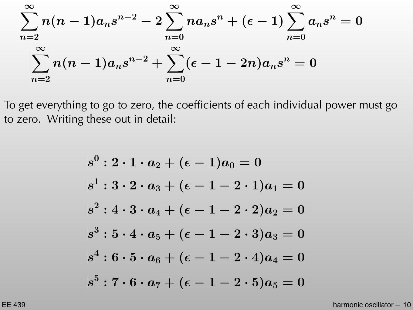
ansn = 0

To get everything to go to zero, the coefficients of each individual power must go to zero. Writing these out in detail:

1X

n=2

n(n � 1)ansn�2 +1X

n=0

(✏ � 1 � 2n)ansn = 0

s0 : 2 · 1 · a2 + (✏ � 1)a0 = 0

s1 : 3 · 2 · a3 + (✏ � 1 � 2 · 1)a1 = 0

s2 : 4 · 3 · a4 + (✏ � 1 � 2 · 2)a2 = 0

s3 : 5 · 4 · a5 + (✏ � 1 � 2 · 3)a3 = 0

s4 : 6 · 5 · a6 + (✏ � 1 � 2 · 4)a4 = 0

s5 : 7 · 6 · a7 + (✏ � 1 � 2 · 5)a5 = 0

10


Note that the even coefficients are connected and the odd coefficients are connected. Once we know ao and a1, we can find all of the higher coefficients using the “recursion relation”:

an+2 =2n + 1 � ✏

(n + 2)(n + 1)an

The first two coefficients, ao and a1, are the arbitrary coefficients that we expect for a second order diff eq.

11


Now for the last detail. We know that the solutions must be bound, and the exp(-s2/2) should guarantee bound functions. However, f(s) consists of an infinitely long power series, it will eventually “overpower” the decaying exponential at sufficiently large values of n. In order to guarantee finite solutions, we must truncate the series to a finite number of terms.

To do that, we can set either ao or a1 to zero, thus removing all the even or all the odd terms. Then, we force the remaining series to truncate by imposing the condition:

✏ = 2n + 1

Now we have the form of the wave functions and the energies. The problem is complete.

E = (2n + 1)~!

2=

✓n +

1

2

◆~!

12


0

(s) = C0

exp

�

s2

2

!

1

(s) = C1

(2s) exp

�

s2

2

!

13

-4 -3 -2 -1 0 1 2 3 4

! (s

)

s = x/L

-4 -3 -2 -1 0 1 2 3 4

! (s

)

s = x/L


2

(s) = C2

�4s2 � 2

�exp

�

s2

2

!

3

(s) = C3

�8s3 � 12s

�exp

�

s2

2

!

14

-4 -3 -2 -1 0 1 2 3 4

! (s

)

s = x/L

-4 -3 -2 -1 0 1 2 3 4

! (s

)

s = x/L

harmonic oscillator - gary tuttle's isu web...

Documents