HARMONIC

INVESTIGATION IN LOW

AND MEDIUM VOLTAGE

NETWORKS USING

COMPUTER SIMULATION

AND MEASUREMENT

DEVICES

Se�an Robert William Egner

A dissertation submitted to the Faculty of Engineering and the Built Envir-

oment, University of the Witwatersrand, Johannesburg, in ful�lment of the

requirements for the degree of Master of Science in Engineering.

Johannesburg, 2006

Declaration

I declare that this dissertation is my own, unaided work, except where other-

wise acknowledged. It is being submitted for the degree of Master of Science in

Engineering in the University of the Witwatersrand, Johannesburg. It has not

been submitted before for any degree or examination in any other university.

Signed this day of 20

Se�an Robert William Egner.

i

Abstract

This dissertation discusses the development of an ATP model of a network

to aid measurement techniques in a harmonic evaluation. A theoretical back-

ground discussion of various pieces of equipment and their signi�cance to har-

monics is included.

National Electricity Regulator (NRS 048) standards are discussed with refer-

ence to performing a basic investigation and short comings. A test study was

performed on the Brandspruit Mine in Secunda.

ATP models are developed for equipment relevant to the test case, these in-

clude AC{AC converters, AC{DC converters, three phase transformers and

cables. Finally the measured test case is compared to simulation results and

conclusions drawn.

ii

Acknowledgements

I would like to thank SASOL and SASOL Mining for the opportunity to study

further and for the support o�ered during the term of my project. Particu-

lary to the Projects & Technology Department for their technical input and

assistance.

Thanks to the School of Electrical Engineering, University of the Witwater-

srand for providing a suitable environment in which to study and to John van Coller

for supervising the project.

I appreciate the e�orts of Andreas Beutel in helping to edit the various drafts

of the dissertation and for helping me with understanding some of the content

covered.

iii

In loving memory of my father

Geo�rey William Egner

1941 - 1993

iv

Contents

Declaration i

Abstract ii

Acknowledgements iii

Contents v

List of Figures xi

List of Tables xiv

List of Symbols xv

List of De�nitions xvi

1 Introduction 1

1.1 Reason for Project . . . . . . . . . . . . . . . . . . . . . . . . . 2

1.2 Document Outline . . . . . . . . . . . . . . . . . . . . . . . . . 2

v

2 Background 4

2.1 Harmonic Sources . . . . . . . . . . . . . . . . . . . . . . . . . 4

2.1.1 AC Motors . . . . . . . . . . . . . . . . . . . . . . . . . 5

2.1.2 Transformers . . . . . . . . . . . . . . . . . . . . . . . . 7

2.1.3 Converter Circuits . . . . . . . . . . . . . . . . . . . . . 10

2.2 Harmonic E�ects . . . . . . . . . . . . . . . . . . . . . . . . . . 12

2.2.1 Resonances . . . . . . . . . . . . . . . . . . . . . . . . . 13

2.2.2 Rotating Machines . . . . . . . . . . . . . . . . . . . . . 15

2.2.3 Static Power Plant . . . . . . . . . . . . . . . . . . . . . 16

2.2.4 System Protection . . . . . . . . . . . . . . . . . . . . . 16

2.2.5 Customer Equipment . . . . . . . . . . . . . . . . . . . . 17

2.2.6 Power Measurements . . . . . . . . . . . . . . . . . . . . 17

2.2.7 Conclusion . . . . . . . . . . . . . . . . . . . . . . . . . . 18

3 Standards and Regulations 19

3.1 NRS 048 { 2: Minimum Standards . . . . . . . . . . . . . . . . 20

3.1.1 Compatibility Levels . . . . . . . . . . . . . . . . . . . . 20

3.1.2 Assessment of Site Harmonics . . . . . . . . . . . . . . . 21

3.2 Evaluation of Measurements . . . . . . . . . . . . . . . . . . . . 22

3.2.1 Ideal Measurement . . . . . . . . . . . . . . . . . . . . . 23

vi

3.2.2 Realistic Measurement . . . . . . . . . . . . . . . . . . . 24

3.2.3 Restrictions and Uses of Measurements . . . . . . . . . . 24

3.3 Shortfall of NRS 048: Current Harmonics . . . . . . . . . . . . . 24

3.4 Conclusion . . . . . . . . . . . . . . . . . . . . . . . . . . . . . . 26

4 Equipment Modelling 27

4.1 Modelling Pre-Process . . . . . . . . . . . . . . . . . . . . . . . 28

4.1.1 Required Information . . . . . . . . . . . . . . . . . . . . 28

4.1.2 Guidelines . . . . . . . . . . . . . . . . . . . . . . . . . . 28

4.1.3 Modelling Tools . . . . . . . . . . . . . . . . . . . . . . . 29

4.2 Modelling of AC { AC Converter Circuits . . . . . . . . . . . . 29

4.2.1 VSD Test Setup . . . . . . . . . . . . . . . . . . . . . . . 30

4.2.2 Basic Model of VSD . . . . . . . . . . . . . . . . . . . . 30

4.2.3 Evaluation of the VSD model . . . . . . . . . . . . . . . 32

4.2.4 Final VSD Model . . . . . . . . . . . . . . . . . . . . . . 35

4.3 AC {DC Converter Circuits . . . . . . . . . . . . . . . . . . . . 36

4.3.1 Basic Model of Chopper . . . . . . . . . . . . . . . . . . 37

4.3.2 Chopper Model Evaluation . . . . . . . . . . . . . . . . . 38

4.4 Transformer . . . . . . . . . . . . . . . . . . . . . . . . . . . . . 39

4.4.1 Model Con�rmation . . . . . . . . . . . . . . . . . . . . 40

vii

4.5 Cable Modelling . . . . . . . . . . . . . . . . . . . . . . . . . . . 44

4.5.1 Model Con�rmation . . . . . . . . . . . . . . . . . . . . 45

4.6 Induction Machine Modelling . . . . . . . . . . . . . . . . . . . 45

4.6.1 Parameter Calculation . . . . . . . . . . . . . . . . . . . 46

4.7 Conclusion . . . . . . . . . . . . . . . . . . . . . . . . . . . . . . 47

5 Network Analysis 49

5.1 Brandspruit Colliery . . . . . . . . . . . . . . . . . . . . . . . . 49

5.1.1 Plant Description . . . . . . . . . . . . . . . . . . . . . . 50

5.1.2 Expansions and Alterations . . . . . . . . . . . . . . . . 50

5.2 Resonance Pre { Study . . . . . . . . . . . . . . . . . . . . . . . 51

5.2.1 Implications . . . . . . . . . . . . . . . . . . . . . . . . . 52

5.3 NRS 048 Evaluation . . . . . . . . . . . . . . . . . . . . . . . . 52

5.3.1 Measurement Devices . . . . . . . . . . . . . . . . . . . . 52

5.3.2 Data Analysis . . . . . . . . . . . . . . . . . . . . . . . . 56

5.3.3 Comments . . . . . . . . . . . . . . . . . . . . . . . . . . 56

5.4 ATP Simulation . . . . . . . . . . . . . . . . . . . . . . . . . . . 58

5.4.1 Problems Encountered . . . . . . . . . . . . . . . . . . . 59

5.4.2 Simulation Analysis . . . . . . . . . . . . . . . . . . . . . 59

5.4.3 Model Con�rmation . . . . . . . . . . . . . . . . . . . . 60

viii

5.4.4 Comments . . . . . . . . . . . . . . . . . . . . . . . . . . 61

5.5 Auto { Switching Capacitor Bank Study . . . . . . . . . . . . . . 61

5.6 Investigation Conclusion . . . . . . . . . . . . . . . . . . . . . . 65

5.7 Conclusion . . . . . . . . . . . . . . . . . . . . . . . . . . . . . . 65

6 Hybrid Evaluation 67

6.1 Initial Analysis . . . . . . . . . . . . . . . . . . . . . . . . . . . 67

6.2 Network Modelling . . . . . . . . . . . . . . . . . . . . . . . . . 68

6.3 Conclusion . . . . . . . . . . . . . . . . . . . . . . . . . . . . . . 69

7 Conclusion 71

References 73

A Transformer Model Calculations 76

B Cable Data 78

C Resonance Calculations 79

C.1 Machine Equivalent Circuits . . . . . . . . . . . . . . . . . . . . 79

C.1.1 Induction Motors . . . . . . . . . . . . . . . . . . . . . . 79

C.1.2 Transformer . . . . . . . . . . . . . . . . . . . . . . . . . 80

C.2 Network Reduction . . . . . . . . . . . . . . . . . . . . . . . . . 81

ix

D Excel Macro Code 86

x

List of Figures

2.1 Transformer magnetisation, excluding hysteresis . . . . . . . . . 7

2.2 Transformer magnetisation, including hysteresis . . . . . . . . . 8

2.3 Symmetrical three phase transformer core . . . . . . . . . . . . 9

2.4 Ideal 6 pulse recti�cation circuit . . . . . . . . . . . . . . . . . . 11

2.5 Six pulse recti�cation waveforms . . . . . . . . . . . . . . . . . . 11

2.6 Series resonance circuit . . . . . . . . . . . . . . . . . . . . . . . 14

3.1 Example of incomer voltage harmonics . . . . . . . . . . . . . . 23

3.2 Example of incomer current harmonics . . . . . . . . . . . . . . 25

4.1 Measured line current . . . . . . . . . . . . . . . . . . . . . . . . 30

4.2 Harmonic spectrum of measured current waveform . . . . . . . . 31

4.3 VSD model equivalent circuit . . . . . . . . . . . . . . . . . . . 32

4.4 Supply { impedance { simulation current waveform . . . . . . . . 33

4.5 Harmonic spectrum of simulated current waveform . . . . . . . 34

4.6 Simulated 2% unbalance current waveform . . . . . . . . . . . . 34

4.7 Harmonic spectrum of simulated current waveform . . . . . . . 35

xi

4.8 VSD base module . . . . . . . . . . . . . . . . . . . . . . . . . . 36

4.9 Basic recti�er and chopping circuit . . . . . . . . . . . . . . . . 36

4.10 Chopper output voltage . . . . . . . . . . . . . . . . . . . . . . 37

4.11 DC machine equivalent circuit . . . . . . . . . . . . . . . . . . . 38

4.12 DC armature parameter measurement . . . . . . . . . . . . . . . 38

4.13 Simulated chopper output voltage . . . . . . . . . . . . . . . . . 39

4.14 � { � transformer HT and LT line currents . . . . . . . . . . . 41

4.15 Simulated LT line current . . . . . . . . . . . . . . . . . . . . . 42

4.16 Simulated HT line current . . . . . . . . . . . . . . . . . . . . . 43

4.17 Simulated HT line current, including source impedance . . . . . 43

4.18 Nominal Pi Cable Model . . . . . . . . . . . . . . . . . . . . . . 44

4.19 Cable Geometry . . . . . . . . . . . . . . . . . . . . . . . . . . . 45

4.20 Induction Machine Equivalent Circuit . . . . . . . . . . . . . . . 46

4.21 Induction Motor Data Program . . . . . . . . . . . . . . . . . . 48

5.1 Substation evaluation . . . . . . . . . . . . . . . . . . . . . . . . 55

5.2 Measured Voltage Harmonic Spectrum . . . . . . . . . . . . . . 57

5.3 Measured Current Harmonic Spectrum . . . . . . . . . . . . . . 57

5.4 Simulated Current Harmonic Spectrum . . . . . . . . . . . . . . 60

5.5 Single Line Diagram of Network . . . . . . . . . . . . . . . . . . 62

5.6 Current Harmonic Signature of 600 kVAr Capacitor . . . . . . . 63

xii

5.7 Current Harmonic Signature of 1200 kVAr Capacitor . . . . . . 64

5.8 Current Harmonic Signature of 1800 kVAr Capacitor . . . . . . 64

6.1 Current Supplied to Capacitor . . . . . . . . . . . . . . . . . . . 69

C.1 Equivalent Circuit of Induction Motor . . . . . . . . . . . . . . 80

C.2 Equivalent Circuit of a Transformer . . . . . . . . . . . . . . . . 81

C.3 Bus Bar 1 Reduction . . . . . . . . . . . . . . . . . . . . . . . . 82

C.4 Bus Bar 2 Reduction . . . . . . . . . . . . . . . . . . . . . . . . 82

C.5 Bus Bar 3 Reduction . . . . . . . . . . . . . . . . . . . . . . . . 83

C.6 Bus Bar 4 Reduction . . . . . . . . . . . . . . . . . . . . . . . . 83

C.7 Bus Bar 5 Reduction . . . . . . . . . . . . . . . . . . . . . . . . 83

C.8 Bus Bar 6 Reduction . . . . . . . . . . . . . . . . . . . . . . . . 84

C.9 Reduced Circuit for Calculation of Resonant Frequency at Sur-

face PFC . . . . . . . . . . . . . . . . . . . . . . . . . . . . . . . 84

xiii

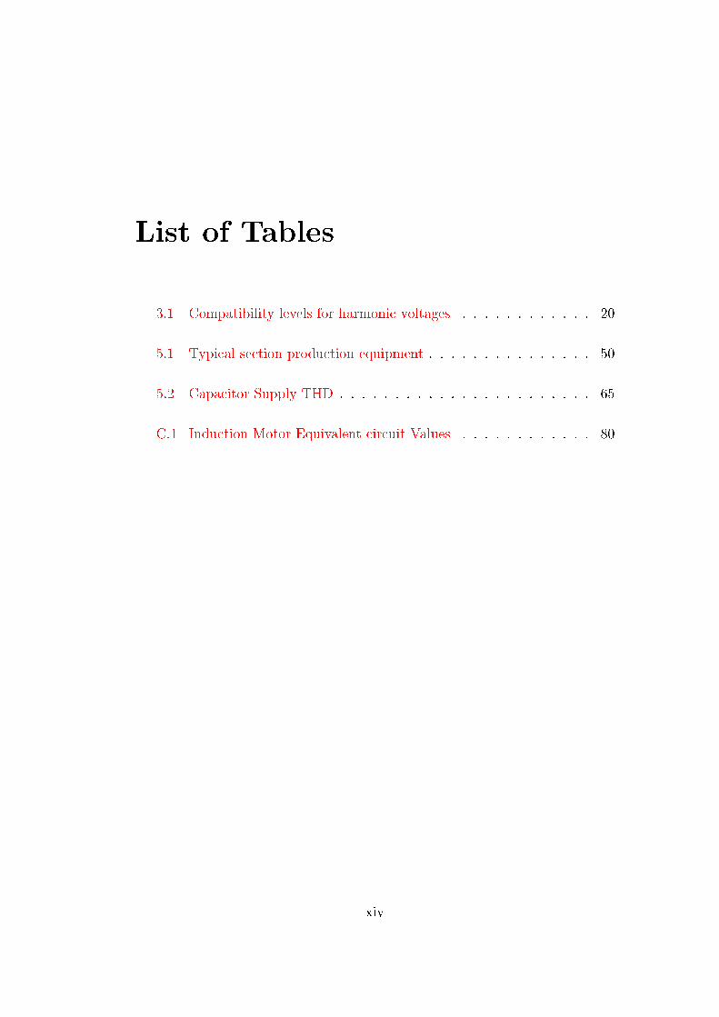
List of Tables

3.1 Compatibility levels for harmonic voltages . . . . . . . . . . . . 20

5.1 Typical section production equipment . . . . . . . . . . . . . . . 50

5.2 Capacitor Supply THD . . . . . . . . . . . . . . . . . . . . . . . 65

C.1 Induction Motor Equivalent circuit Values . . . . . . . . . . . . 80

xiv

List of Symbols

kd Distribution factor for synchronous machine armature wind-

ings

ks Coil-span factor for synchronous machine armature winding

Vh The percentage r.m.s. value of the hth harmonic or interhar-

monic voltage component

xv

List of De�nitions

ADC Analogue to Digital Converter

ATP Alternative Transients Program, computer simula-

tion package

CT Current Transformer

Customer Anyone whom purchases electricity from the na-

tional supplier

e.m.f. Electromotive Force

Even Harmonics Harmonics of an even (divisible by two) order

FFT Fast Fourier Transform

HT High Tension; of higher voltage

HV The set of nominal voltage levels that are used in

power systems for bulk transmission of electricity

in the range 44 kV < Un � 220 kV

IGBT Insulated Gate Bipolar Transistor

Interharmonics Frequency components which are not an integral

multiple of the fundamental frequency

LCC Line and Cable Constants program, an ATP mod-

ule

LT Low Tension; of lower voltage

xvi

LV Low voltage, the set of nominal voltage levels that

are used for the distribution of electricity and

whose upper limit is generally accepted to be an

a.c. voltage of 1000 V

m.m.f. Magnetomotive Force

MV Medium Voltage, the set of nominal voltage levels

that lie between low and high voltage in the range

1 kV < Un � 44 kV

NER National Electricity Regulator

NRS National Regulator Standards

Odd Harmonics Harmonics of an odd (not divisible by two) order

PCC Point of Common Coupling, the point in a network

where more than one customer will be connected

or is connected

PC Personal Computer

PFC Power Factor Correction

QoS Quality of Supply

r.m.s. Root{Mean{Square

SCR Silicon Controlled Recti�er

THD Total Harmonic Distortion

Triplen Harmonics Harmonics of an order which is a multiple of three

Torque A turning or twisting; tendency to turn, or cause

to turn, about an axis.

UPS Uninterruptible Power Supply

VSD Variable speed drive (in this text it will refer to

AC{AC type drives)

xvii

VT Voltage Transformer

XLPE Cross { Linked Polyethylene

xviii

Chapter 1

Introduction

Harmonic pollution is commonplace in electrical networks. Harmonics are gen-

erated by various pieces of equipment which are in use. In order to structure

an electrical network to minimise harmonic propagation and e�ect, an under-

standing of how and where they are created is needed. From this understanding

it is possible to avoid situations where harmonic propagation is accentuated.

Background harmonics exist on all networks, they are small and for all intents

and purposes can be ignored. However, industry today makes use of vari-

ous pieces of equipment, including VSDs and PCs, which generate additional

harmonics.

Any expanding electrical network could experience maloperation due to har-

monic e�ects. It is important to be able to predict the harmonic consequences

of any changes or expansions to a network. A combination of measurements

and computer simulation can be used to predict such consequences.

As the use of switch {mode powers supplies, converters and other harmonic

producing equipment grows, the need to minimise the e�ects of the harmonics

becomes of greater importance. This is because harmonic distortion of voltages

in networks a�ects the operation of equipment as well as the electrical rating

of equipment [1].

This project investigates the sources of harmonics in electrical networks, the

1

e�ect of harmonics on the networks and methods to measure and predict them.

1.1 Reason for Project

Although there are government standards which deal with power quality and

harmonics, the standards are based on supplier guidelines as opposed to cus-

tomer guidelines. A customer has few guidelines for structuring his network

to minimise the e�ect of harmonics on his equipment.

The project evaluates NRS 048 limits as an e�ective means of evaluating a

customer network and making recommendations regarding the e�ect of future

installations and alterations to the network.

1.2 Document Outline

This document details an investigation into the causes and e�ects of power

system harmonics, as well as the measurement and simulation of power system

harmonics.

The network studied was that of the Brandspruit Colliery, SASOL Mining,

Secunda. The colliery was chosen as the test subject because of its continually

expanding operations. As the coal is mined, the electrical network expands,

changing its electrical characteristics.

A harmonic study, in accordance with government standards [2], of the live

electrical network was performed. An ATP simulation of the plant was then

compiled.

The correlation between the simulation results and measurements are dis-

cussed, as well as the pros and cons of each technique.

2

A proposed hybrid solution, combining both measurement and simulation tech-

niques, is also discussed as a set of guidelines for harmonic evaluation of in-

dustrial networks.

3

Chapter 2

Background

Power system harmonics are de�ned as sinusoidal voltage and currents at fre-

quencies that are integer multiples of the main generated (fundamental) fre-

quency. They constitute the major distorting components of the mains voltage

and load current waveforms [3].

Harmonic pollution in reticulation networks is becoming more widespread with

the development and introduction of industrial processes which rely upon vari-

able speed drives and other non-linear loads for their operation. Although the

e�ect of harmonics has been noted, the onus is on the customer to take pre-

ventative measures and not the supplier.

This chapter discusses harmonic sources and their e�ects which occur in in-

dustrial networks. Individual pieces of equipment are discussed with reference

to how they produce harmonics and what preventative measures can be taken

to minimise their e�ects.

2.1 Harmonic Sources

Typical harmonic sources found on an industrial network include

� AC Motors

4

{ Synchronous

{ Induction

� Transformers

� Recti�er circuits

{ Charging stations: for battery operated vehicles

{ Network capacitance and inductance (resonance)

{ VSDs

Each of these sources is individually discussed in the following subsections.

2.1.1 AC Motors

An AC motor is a machine designed to transform electrical energy into kinetic

energy. Electric machines are made up of interlinked electric and magnetic

circuits. Interaction between the resultant electric currents and magnetic �elds

in motors results in an electromechanical energy conversion.

Rotating machines inherently generate harmonics, due in part to winding

methods and slotting e�ects. It can be shown [1] that a three phase wind-

ing will not generate any triplen harmonics but will develop 5th and 7th order

harmonics. The 5th is found to travel in a negative direction whilst the 7th is

found to travel in a positive direction.

The construction methods used to make electric motors require that slots be

created to house the windings, these slots result in an inconsistent airgap

thickness which is referred to as slotting. Slotting e�ects cause the resultant

machine m.m.f. wave to modulate because of permeance variation in the air

gap/slot region. The permeance change can be approximated by

A1 +A2 sin

�2mg

2�x

�

�(2.1)

5

whereA1 = the base permeance

A2 = the max permeance change

mg = the number of slots per pole

x = the o�set from \0" position

� = fundamental wavelength

Discussion of harmonic generation by each of the two subgroups of AC motor,

namely synchronous and induction machines follows.

Synchronous Machines

A synchronous machine operates at constant speed and frequency under steady

state conditions [4]. They are used in applications where constant speed is

critical. Synchronous machines are also extensively used for power generation.

Flux is not evenly distributed across the poles of a synchronous machine, es-

pecially in a salient pole design. The e�ective electrical phase spread of the

winding, coil span and interphase connection determine the magnitude of e.m.f.

harmonics within the armature.

Through the selection of a suitable distribution angle, kd, and coil-span factor,

ks, it is possible to minimise or even eliminate e.m.f. harmonics. Phase connec-

tion (star or delta) will eliminate triplen harmonics in a three phase machine

and is often used to do so. Coil-span is used to reduce the �fth and seventh

harmonics [1].

Induction Machines

Induction motors are the most commonly used motors in industry today. They

are used for applications which do not require a high degree of speed consist-

ency. An induction motor operates at a speed slightly lower than synchronous

speed. The amount of slip experienced by the motor is dependant on the

machine loading, larger loads will result in a lower speed.

6

The rotating �eld of an induction motor stator has a synchronous speed of

fundamental frequency times wavelength (f1�). The rotor speed is a function

of the motor slip and is f1�(1� s), the rotor current has a frequency of sf1.

A rotor m.m.f. harmonic of order n has a wavelength of �=n, a speed of sf � �=nwith respect to the rotor or f�(1 � s) + (sf)�=n with respect to stator. The

wave can travel in either a positive or negative direction with respect to the

fundamental.

The e.m.f. induced by this harmonic is equal to the ratio of speed to wavelength,

which simpli�es to:

e.m.f.n = f(n� s(n+ 1)) (2.2)

2.1.2 Transformers

Transformers are made up of electric and magnetic circuits, similar to those

found in AC motors, however through the interaction of the resultant mag-

netic �elds and electric currents an electrical energy transfer is created [4].

Transformers are used to step { up or step { down voltages within a network.

The primary current, in a transformer, is not purely sinusoidal, because the

ux is not linearly proportional to magnetising current. As a transformer core

becomes saturated a smaller ux change is required to generate a large primary

current change, see Figure 2.1.

Figure 2.1: Transformer magnetisation, no hysteresis [1]

7

Figure 2.2 shows the e�ects of hysteresis 1 on the primary current. It can be

seen that the magnetising current is no longer symmetrical around its max-

imum value.

The deformed (non { sinusoidal) current waveforms shown in Figures 2.1 and 2.2,

consist of mainly triplen harmonics, particularly the third [1]. In order to min-

imise these triplen harmonics it is necessary to provide a current path for them,

this is achieved by delta connecting the winding [6].

It is also possible to reduce the triplen harmonic m.m.f. through the use of

three-limbed transformers. Triplen harmonics ow in the same direction in

each limb, hence they are additive and the only return path is through the

transformer oil and case [1]. This will maintain sinusoidal e.m.f. and ux

density waveforms.

The e�ects of the magnetising current harmonics can be ignored as the trans-

former is loaded up because the magnetising current is approximately 0.05 p.u

of the full load current in large transformers [5]. Transformers are likely to

experience these problems most signi�cantly when the system is lightly loaded

and the voltage is high [1].

1The rising section of hysteresis curve is used for the rising section of the magnetising

current curve.

Figure 2.2: Transformer magnetisation, including hysteresis [1, 5]

8

It should be noted that �fth and seventh order harmonics are not corrected

by these methods and should not be ignored. In order to suppress the �fth

and seventh harmonics two transformers in parallel can be used, one should be

delta-delta wound and the other star-star wound. Fifth and seventh harmonics

will be produced which are equal in magnitude but opposite in phase, hence

cancelling them from the combined input.

It is possible to create this cancelling e�ect in one transformer by providing

a magnetic circuit which contains both a star and a delta path, as shown in

Figure 2.3. A �fth and seventh harmonic excitation occurs in the two yokes

(unwound) which are in phase opposition to the limb they are magnetically

connected to. This e�ect is inherent in a �ve-limb transformer, which if the

outer, unwound limbs were joined would create the same symmetrical shape

as in Figure 2.3 [6].

Figure 2.3: Symmetrical three phase transformer core [5]

9

2.1.3 Converter Circuits

Converter circuits are used to \create" alternative supplies. Typically, supplied

voltage is converted to a similar voltage but with a di�erent frequency. This is

done by converting an AC voltage to DC, and then converting (reverse process)

the DC to a required voltage and frequency.

A six pulse recti�cation circuit is obtained using a con�guration similar to that

shown in Figure 2.4. This is a simpli�ed version of actual six pulse recti�cation,

due to the fact that only diodes are used and all elements are assumed to be

ideal, there is also no diode ignition voltage including in the representation.

The line voltages are shown in Figure 2.5(a) and the phase currents in Fig-

ure 2.5(b), (c) and (d). From Figures 2.4 and 2.5 it is possible to see which

diodes conduct at what times during a full period.

In analysing the phase current ia, of Figure 2.5(b), it can be seen that the

positive section is the current component owing through diode 1 (i1), whilst

the negative section is the current owing through diode 4 (�i4, where j i4j =j i1j). The current waveform coincides with the voltage waveform, Va. The

phase current ia is found to be void of any triplen harmonics and can be

represented by equation 2.3:

ia =2p3

�Id(cos!t� 1

5cos 5!t+

1

7cos 7!t� 1

11cos 11!t

+1

13cos 13!t� 1

17cos 17!t+

1

19cos 19!t� : : :)

(2.3)

whereia = a phase current

Id = the DC current

It should also be noted that all the current that ows through a diode will

return through two others at di�erent times; for example current through

diode 1 will return through either diode 5 (as in time section 1) or diode 6 (as

in time section 6), it does not return through both diode 5 and diode 6 at the

10

i 1 i 2 i 3

i 4 i 5 i 6

i a

i b

i c

V DC

1 2 3

4 5 6

Figure 2.4: Ideal 6 pulse recti�cation circuit

0

0

0

0

0

VABVBC VCA

Diode 4

Diode 1 Diode 1

Diode 2

Diode 5 Diode 5

Diode 3

Diode 6

ia

ib

ic

1 2 3 4 5 6 7

(a)

(b)

(c)

(d)

(e) IA

Figure 2.5: Six pulse recti�cation waveforms: (a) line voltages (b) - (d) phase

currents (e) phase current on a �� � transformer

11

same time.

When a delta { star transformer is used to connect to the bridge circuit, the

phase current on the primary side of the transformer becomes the scaled in-

stantaneous di�erence between two secondary currents (Figures 2.5(b), (c) and

(d)) as shown in Figure 2.5(e) [6].

Each individual type of conversion, AC { AC or AC { DC, will have a

speci�c circuit depending on its application. An AC { AC converter will

include an inverter (either SCR or IGBT on the output of the recti�er, the

inverter will be controlled to create the required AC frequency. An AC {

DC converter may use a chopping circuit to reduce the DC voltage to the

required value. These con�gurations e�ect the method in which the converter

is modelled harmonically.

2.2 Harmonic E�ects [1]

The main e�ects of voltage and current harmonics in power systems are:

� Increased losses in power generation, transmission and utilisation

� Ageing of the insulation of electrical plant components and thus a shortened

useful life

� Maloperation or unexpected operation of the plant

� Mis�ring of thyristors and other gating circuits

Another ill-e�ect of harmonics is ampli�cation due to series and parallel reson-

ances, between network capacitance and inductance. These resonance e�ects,

between various pieces of equipment, can result in hunting 2 and over-voltage.

It is expensive to take preventative measures, since each network will be unique

and a custom solution devised, and therefore most understanding has come

2When a motor varies its speed to track changing supply frequency

12

from post-disaster analysis. Further, taking measurements is di�cult as the

harmonics are not continuous and vary subject to load, time and other equip-

ment on the network.

2.2.1 Resonances

Resonance is de�ned as \A phenomenon in which a vibration or other cyclic

process (such as tide cycles) of large amplitude is produced by smaller impulses,

when the frequency of the external impulses is close to that of the natural

cycling frequency of the process in that system [7]."

The combination of network capacitance and inductance causes resonance.

The resultant ampli�ed harmonic currents can over-stress capacitors, which

will shorten the useful life of the capacitors.

Common sources of inductance are:

� Transformers

� Cables and overhead lines

Common sources of capacitance are:

� Power factor correction capacitors

� Harmonic �lters

� Undamped surge capacitors

� Cables

Parallel resonance causes increased harmonic voltages and high harmonic

currents in the legs of the parallel impedance, since many harmonic sources are

e�ectively current sources. This can occur in various ways, the most common

13

Transformer (S t , VA) Nonlinear

Load

Capacitor Bank

(S c , VA r )

Resistive Load

(S L , VA)

Figure 2.6: Series resonance circuit

being when a capacitance is connected to the same busbar as an harmonic

source (normally inductive).

The series resonant condition, shown in Figure 2.6, is of concern because for

relatively low harmonic voltage, high capacitor currents can ow, depending

on the quality factor, Q, of the circuit. At high frequencies the load resist-

ance becomes negligible as the capacitive reactance decreases (impedance is

inversely proportional to frequency).

Should a load current harmonic be likely to have a frequency near the resonant

frequency of the circuit then untuned power factor correction capacitors should

be replaced with tuned capacitor banks (i.e. they should include a series

inductance), which will alter the resonant frequency of the circuit [8].

A good practice is to only use untuned capacitors when no large non-linear

loads are to be fed from the same supply. It is unlikely that resonance will

occur with only linear load (no harmonics), and so it is not necessary to alter

the resonance frequency.

14

2.2.2 Rotating Machines

Harmonics in a rotating machine have various e�ects, one is an increase in ma-

chine windage losses. The other is the creation of undesired torque pulsations.

A discussion of each of these follows.

Losses

Harmonic voltages or currents cause additional power losses to be experienced

in the rotor and stator windings as well as in the rotor and stator laminations.

These additional losses are due to eddy current and skin e�ects, the greatest

of which occur in the rotor. These additional power losses are probably the

most serious e�ect of the harmonics. This conclusion can be extended to

synchronous machines.

A machine's ability to deal with the additional harmonics will depend on the

total additional losses and their local (rotor) and overall heating e�ects. The

probable acceptable levels will be indicated by the level of continuous negative

sequence current limitation of the machine (10% for generators and 2% for

induction machines).

Torques

Additional harmonic torques can be produced by harmonic currents owing

in the stator windings of induction machines. This motoring action causes

shaft torques in the direction of the harmonic �eld. The harmonics tend to

cause torques in pairs, which cancel each other. The mean torque is essentially

una�ected, although signi�cant torque pulsations are created.

15

2.2.3 Static Power Plant

The various parts of the plant are all a�ected by harmonics. The major, noted,

e�ect is the shortening of the useful life-span of equipment. Transmission lines

su�er from increased losses, and hence additional heating, due to the increased

r.m.s current.

Corona inception voltage could be exceeded due to the possible increase in the

wave peak value (in the case of synchronised harmonics). Despite the r.m.s

voltage being below the inception value the peak value may still exceed the

maximum possible value.

Transformers experience increased hysteresis, eddy current losses and insula-

tion stress. Increased copper losses cause unexpected hot spots and require

increased ratings.

Usually, the �rst components [8] to be a�ected by harmonics are the power

factor correction capacitors. Increasing frequencies cause the impedance of

the capacitors to decrease (Z = 1j!C

). This causes susceptibility to current

overloading and heating in the case of higher order harmonics. The result of

these e�ects is nuisance tripping, failure and overheating.

2.2.4 System Protection

Distorted or degraded operating characteristics of protective relays can result

from harmonics. Digital relays and algorithms, especially those dependant on

sampling or zero crossing are particularly sensitive, as the waveform monitored

is not purely sinusoidal (For example a distance protection relay).

In cases where the harmonic distortion is under 20%, the changed operating

characteristics present no problems, as the devices are robust enough to cope

with the distortion. However with the increasing use of large power converters,

the harmonic levels may exceed this acceptable level.

16

2.2.5 Customer Equipment

The following customer equipment can be a�ected by harmonics:

� Television receivers : Varying picture size and brightness result from har-

monics which e�ect peak voltage.

� Florescent and mercury arc lighting : The capacitance in the ballast de-

velops a resonant frequency with the inductance of the ballast and circuit.

If the general harmonics correspond to the resonant frequency, excessive

heating and therefore failure may result.

� Thyristors : Mis�ring due to notching. Unexpected �ring of the gating

circuits.

� Fuses : Unnecessary failure caused by harmonic heating e�ects [8].

� Surge arrestors : Overvoltage stresses cause premature failure [8].

2.2.6 Power Measurements

Harmonics can a�ect measurement equipment both positively (increasing the

measurement) and negatively (decreasing the measurement). This is due to

the device being calibrated on a pure sinusoidal waveform. Harmonic voltages

or currents reduce the ability of the meter 3 to measure fundamental frequency

power.

In general, it has been found that the meters will measure high, imposing an

extra cost to the consumer. This is due to the fact that harmonics are generally

re ected as a higher electricity consumption, hence penalising the consumer.

3Ferraris motor type kilowatt{hour meter

17

2.2.7 Conclusion

This chapter clari�ed some typical harmonic sources in industrial networks.

Although the list is not exhaustive it gives a clear indication of what equip-

ment can cause harmonics and why. The e�ects of harmonics on industrial

equipment and consumer equipment is also highlighted.

From this chapter it is clear that harmonics are an aspect of concern and an

estimate of the distortion in a network is of great importance. By understand-

ing the harmonics generated in a network and their e�ect on equipment within

the network, one is better able manage and operate it.

18

Chapter 3

Standards and Regulations

Harmonics are an inevitable fact of modern equipment used in industry and

hence standards are stipulated in order to control the level of voltage and

current distortion. The standards enforce a QoS that is suitable for both users

and suppliers.

There are various approaches to this problem. South Africa has adopted an

approach which stipulates the voltage harmonic distortion permissible at the

PCC, i.e. the maximum distortion levels that a supplier may supply to a

customer.

Other countries have stipulated the levels of distortion a customer may cause

to the suppliers network, for example the United Kingdom, have adopted an

approach which regulates the equipment that may be connected to the network,

dependant on the size and type of machine and the distortion already present

at the PCC [9, 10].

The NRS 048 suite of documents is the South African NERs standard on

power quality, it deals with voltage harmonics and interharmonics, voltage

icker, voltage unbalance, voltage dips, voltage regulation and frequency [2,

11, 12, 13, 14].

19

3.1 NRS 048 { 2: Minimum Standards

Guidelines created for the NER stipulate minimum compatibility levels, as-

sessed levels and assessment methods for use by suppliers. These guidelines

are typically followed by users, as they represent conditions under which equip-

ment will continue to operate as expected.

3.1.1 Compatibility Levels

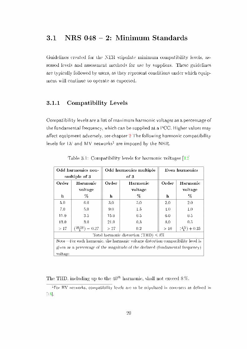
Compatibility levels are a list of maximum harmonic voltages as a percentage of

the fundamental frequency, which can be supplied at a PCC. Higher values may

a�ect equipment adversely, see chapter 2 The following harmonic compatibility

levels for LV and MV networks1 are imposed by the NER.

Table 3.1: Compatibility levels for harmonic voltages [12]

Odd harmonics non- Odd harmonics multiple Even harmonics

multiple of 3 of 3

Order Harmonic Order Harmonic Order Harmonic

voltage voltage voltage

h % h % h %

5.0 6.0 3.0 5.0 2.0 2.0

7.0 5.0 9.0 1.5 4.0 1.0

11.0 3.5 15.0 0.5 6.0 0.5

13.0 3.0 21.0 0.3 8.0 0.5

> 17 ( 38:59h

)� 0:27 > 27 0:2 > 10 ( 2:5h) + 0:25

Total harmonic distortion (THD) � 8%

Note { For each harmonic, the harmonic voltage distortion compatibility level is

given as a percentage of the magnitude of the declared (fundamental frequency)

voltage

The THD, including up to the 40th harmonic, shall not exceed 8%.

1For HV networks, compatibility levels are to be stipulated in contracts as de�ned in

[13].

20

3.1.2 Assessment of Site Harmonics [12]

All supply phases must be monitored. For solidly earthed star connected sys-

tems phase { to { earth voltages should be measured. Phase { to { phase voltages

must be measured in delta connected systems, impedance earthed or unearthed

systems.

An assessment must be conducted over a continuous seven day period, which

should cover a complete cycle of shifts and typical network operating modes.

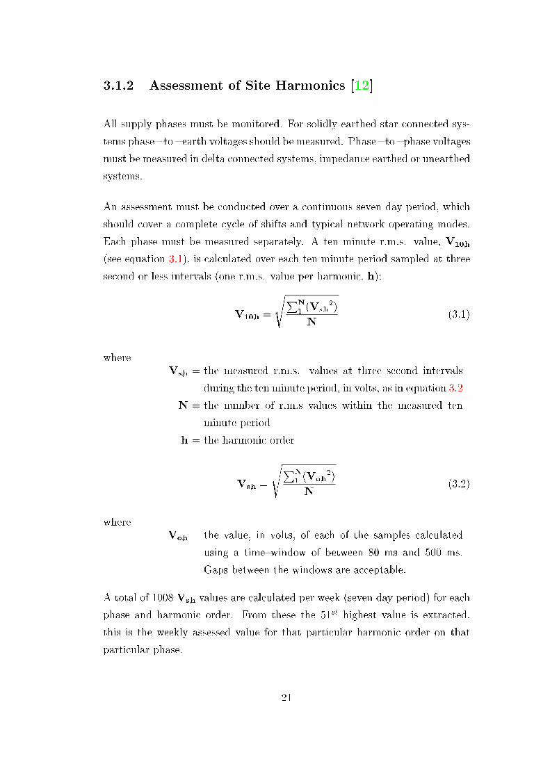
Each phase must be measured separately. A ten minute r.m.s. value, V10;h

(see equation 3.1), is calculated over each ten minute period sampled at three

second or less intervals (one r.m.s. value per harmonic, h):

V10;h =

sPN

1 (Vs;h2)

N(3.1)

whereVs;h = the measured r.m.s. values at three second intervals

during the ten minute period, in volts, as in equation 3.2

N = the number of r.m.s values within the measured ten

minute period

h = the harmonic order

Vs;h =

sPN

1 (Vo;h2)

N(3.2)

whereVo;h = the value, in volts, of each of the samples calculated

using a time{window of between 80 ms and 500 ms.

Gaps between the windows are acceptable.

A total of 1008 Vs;h values are calculated per week (seven day period) for each

phase and harmonic order. From these the 51st highest value is extracted,

this is the weekly assessed value for that particular harmonic order on that

particular phase.

21

This is repeated for all three phases, the highest value of the 95% non-

exceedence levels for each phase, is then considered to be the assessed weekly

value for that particular harmonic on all three phases (95% non-exceedence

level for a particular harmonic for the worst phase).

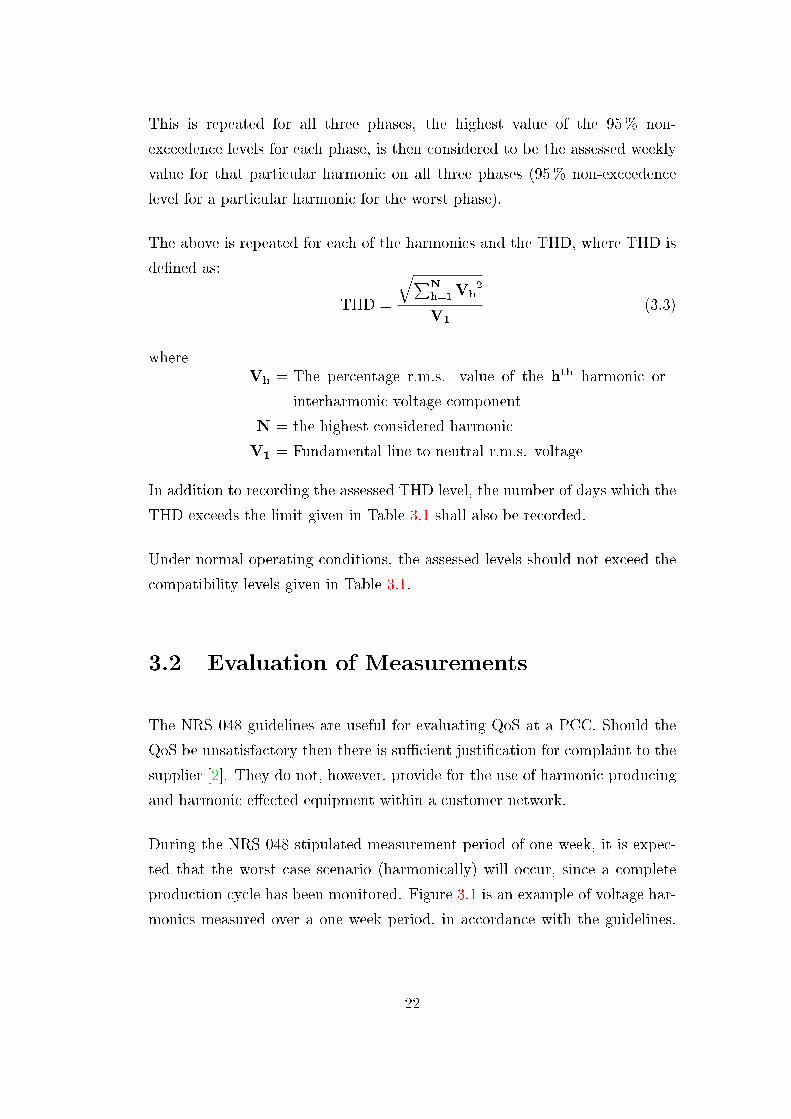
The above is repeated for each of the harmonics and the THD, where THD is

de�ned as:

THD =

qPN

h=1Vh2

V1

(3.3)

whereVh = The percentage r.m.s. value of the hth harmonic or

interharmonic voltage component

N = the highest considered harmonic

V1 = Fundamental line to neutral r.m.s. voltage

In addition to recording the assessed THD level, the number of days which the

THD exceeds the limit given in Table 3.1 shall also be recorded.

Under normal operating conditions, the assessed levels should not exceed the

compatibility levels given in Table 3.1.

3.2 Evaluation of Measurements

The NRS 048 guidelines are useful for evaluating QoS at a PCC. Should the

QoS be unsatisfactory then there is su�cient justi�cation for complaint to the

supplier [2]. They do not, however, provide for the use of harmonic producing

and harmonic e�ected equipment within a customer network.

During the NRS 048 stipulated measurement period of one week, it is expec-

ted that the worst case scenario (harmonically) will occur, since a complete

production cycle has been monitored. Figure 3.1 is an example of voltage har-

monics measured over a one week period, in accordance with the guidelines.

22

Figure 3.1: Example of incomer voltage harmonics

This worst case should be lower than the maximum permissible values stipu-

lated by the NER [12], see Table 3.1.

3.2.1 Ideal Measurement

The ideal measurement occurs when the network harmonic voltage levels are

worst, and every point within the network is measured at the same time. This

allows for points with high harmonic content to be identi�ed and evaluated.

The results of such a study could then be used to evaluate the overall harmonic

levels in the network with a view to correcting or preventing adverse harmonic

conditions.

23

3.2.2 Realistic Measurement

Unfortunately most networks are dynamic and cannot be simply manipulated

to generate worst case scenarios. Production cycles, maintenance, equipment

ratings and network size all a�ect the measurement process.

Inevitably normal operating conditions for a network do not require the equip-

ment to operate at its rated values. Rated values are determined to allow for

maximum requirements at any time. For example, a conveyor motor would be

rated to start a fully loaded belt, this eventuality is rare and hence the belt

motor will run continuously at a much lower value than its rating.

3.2.3 Restrictions and Uses of Measurements

The cost and availability of measurement equipment makes it almost im-

possible to measure every point within a network. It is reasonable to assume

that the point of supply can be monitored and some spot measurements within

the network can be made, this will result in an incomplete view being generated

from the readings.

The readings of the PCC will identify times at which the harmonic content

was high, although the source of the harmonics may not be identi�ed, as not

all required information may have been collected.

The measurements are best used as a baseline for modelling purposes and as

a warning of harmonic changes within the network.

3.3 Shortfall of NRS 048: Current Harmonics

Typical consumer power electronics draw a distorted current waveform, these

current harmonics are ignored by NRS 048, which is concerned only with

24

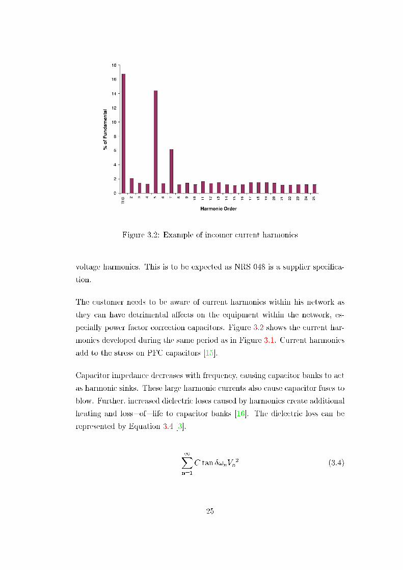
Figure 3.2: Example of incomer current harmonics

voltage harmonics. This is to be expected as NRS 048 is a supplier speci�ca-

tion.

The customer needs to be aware of current harmonics within his network as

they can have detrimental a�ects on the equipment within the network, es-

pecially power factor correction capacitors. Figure 3.2 shows the current har-

monics developed during the same period as in Figure 3.1. Current harmonics

add to the stress on PFC capacitors [15].

Capacitor impedance decreases with frequency, causing capacitor banks to act

as harmonic sinks. These large harmonic currents also cause capacitor fuses to

blow. Further, increased dielectric loses caused by harmonics create additional

heating and loss { of { life to capacitor banks [16]. The dielectric loss can be

represented by Equation 3.4 [3].

1Xn=1

C tan �!nVn2 (3.4)

25

whereC = Capacitance

tan � = the loss factor (tan � = R1=!C

)

!n = angular frequency of nth harmonic

Vn = r.m.s. voltage of nth harmonic

Power factor correction capacitors are often tuned around the third and �fth

harmonic with a small series inductance. This causes the capacitor to appear

inductive to higher frequencies and so prevents parallel resonances [3], since

the capacitive component is negated.

3.4 Conclusion

The NRS 048 standards are issued with the intent to control the levels of

pollution supplied to a customer. They do not explicitly de�ne how a customer

should structure his network, so as to minimise harmonics and their e�ect.

The compatibility levels are based on an maximum harmonic value that can

be tolerated by equipment and so can be used as a guideline for a customers

network.

Current harmonics are of concern with respect to overstressing of PFC capa-

citors and so, although not covered by NRS 048 , are of concern to customers.

26

Chapter 4

Equipment Modelling

A computer model is a mathematical representation of an actual or planned

piece of equipment or network. It is used to simulate actual devices, so that

engineers can predict results and verify theories of equipment or network per-

formance.

Computer simulation is an additional tool that can be used for harmonic pre-

diction. A correctly structured model can simulate situations that cannot be

created in the working environment. Simulation allows an engineer to invest-

igate particular aspects and scenarios which are of interest to whatever study

is performed.

In order to optimise network structure harmonically, harmonic studies evaluate

the worst case scenario, in which the worst possible harmonic content is found

on the network. In reality, it is not always possible to force an active network

into a worst case scenario, normal production cycles do not always allow it.

The worst case scenario is the desired result of an NRS 048 study and is

important when applying the compatibility levels and specifying equipment

capable of dealing with the harmonic content.

Models should be created based on consistent assumptions and should generate

results that are relevant to the study performed. Once a set of guidelines, rules

of model development, have been accepted, it will make development, analysis

and future modi�cation of the models simpler and more e�ective.

27

4.1 Modelling Pre-Process

In order to create a full scale model of a network, it is necessary to have a

complete understanding of the network in question, from the various types of

equipment to the interconnection of said equipment. Circuit diagrams of the

network will provide the basic connections and all the equipment used on the

network.

4.1.1 Required Information

Each device that is to be individually modelled, has its own operating charac-

teristics and electrical structure. The equivalent circuit used to model a device

should be accurate as possible with enough detail to completely simulate the

harmonic content of interest, for example up to the 40 th harmonic, and their

e�ects.

Speci�cations of equipment from the single line diagram, such as transformer

leakage impedance, load sizes and connection (star or delta) will de�ne the

necessary pieces of equipment and the level of detail included in the model.

4.1.2 Guidelines

Network size should be considered when deciding how to model a network,

as larger networks require more time to develop the model and compute the

solutions; and the software available can a�ect the complexity of the model

allowed, e.g limited nodes [17] .

Most consumer networks are built up of similar pieces of equipment, therefore

reducing in { house maintenance training, as technicians have to learn about

fewer machines. Therefore, this practice results in a lower equipment model

count and the repetitive use of models.

28

When creating a new model for a piece of equipment, the model results should

be compared with actual current and voltage measurements taken of the equip-

ment in isolation. The results of the simulation should coincide with the meas-

ured results, thus ensuring the validity of the equivalent circuit and model.

It is not necessary to simulate an original circuit exactly if a simpler equi-

valent circuit is suitable. The use of equivalent circuits will help to optimise

simulation time and minimise complexity.

Models should be optimised to best represent the equipment, and should then

be used as the standard model for that type of equipment throughout the plant

simulation.

4.1.3 Modelling Tools

There are various simulation packages available on the market today. All

packages have a di�erent approach and interface. It is important to select

a package which is a�ordable, comfortable and suitable to the modelling ap-

proach chosen. ATP [18] and ATPDraw [19] were selected for the evaluation

discussed in this report.

Other examples of software include Simulink R [20] and DigSilent R [21].

4.2 Modelling of AC { AC Converter Circuits

Rapid development and therefore increased usage of power electronics, includ-

ing powerful semiconductor devices and microprocessors which are provided in

modular forms, have made the use of variable AC drive technology economic-

ally viable and an alternative to adjustable speed DC drives [22].

This increased usage implies that most industrial networks will have VSDs

connected to them and hence a model will be required.

29

-60

-50

-40

-30

-20

-10

0

10

20

30

40

50

-0.02 -0.015 -0.01 -0.005 0 0.005 0.01 0.015 0.02 0.025 0.03

Time (s)

Curr

ent (

A)

Figure 4.1: Measured line current

4.2.1 VSD Test Setup

An individual VSD was used to determine the waveforms and harmonic con-

tent created by such a drive, when una�ected by other harmonic sources. The

drive was run at full load and the current and voltage waveforms were recorded.

Figure 4.1 shows the current waveform, the high frequency noise can be at-

tributed to the measurement equipment used and the environmental (machines

workshop) noise. The harmonic spectrum is shown in Figure 4.2.

4.2.2 Basic Model of VSD

The basic circuit is shown in Figure 4.3. The capacitor in the DC link in the

recti�er, prevents harmonics produced by the load { side inverter from being

injected back through the diode bridge into the supply [23]. A basic VSD model

was created based on diode technology. A resistive load was connected across

the DC link, the resistance value was chosen such that the power dissipated

was the same as the power consumed by the actual motor connected to the

drive.

30

0

1

2

3

4

5

Abs

mag

nitu

de (A

)

Fourier analysis: Current Waveform

0 2 4 6 8 10 12 14 16 18−100

0

100

200

300

Phas

e (O

from

fund

amen

tal)

Harmonic Order

Figure 4.2: Harmonic spectrum of measured current waveform

A snubber circuit is placed in parallel with each diode, this is to help minimise

transients which are dissipated through the resistive component. The snubber

values used are in accordance with industry standards, with a capacitance of

0:1 �F and resistance of 47 (Labelled RSnub and CSnub in Figure 4.3).

A capacitance across the DC output of the recti�er is used to smooth the

output voltage. The DC link capacitance is a load { speci�c value, there is a

linear relationship between capacitance and load. A recti�er with a DC link

capacitance of 9400 �F for a load of 70 kW was used to determine a value for

the equivalent circuit DC link capacitance [24] (Labelled CSmooth in Figure 4.3).

Non-linear elements in ATP, such as diodes, require a linear element connected

in series either side of it. A small resistor was used for this purpose, the value

of which is 0:003 . They are a requirement of the modelling program and

are not a standard component in any real circuit. Symmetry resistors are used

throughout the modelling process, but have a low enough value so as not to

a�ect the overall result.

31

Figure 4.3: VSD model equivalent circuit

4.2.3 Evaluation of the VSD model

The completed model was tested under various condition to verify its correla-

tion to an actual device. The individual simulations are discussed below.

Balanced Supply Simulation

An initial simulation comprising a balanced three phase supply (without source

impedance) and a VSD was performed. The line current and line voltage were

measured. It was found that the voltage did not visibly deviate from a 50 Hz

sine wave. The current was found to have a similar waveform as that measured

in Figure 4.1.

Supply Impedance Simulation

A more realistic evaluation would include a supply impedance which naturally

occurs in real networks. A supply impedance was chosen, assuming a 10 kA

fault level with an angle of 30 �. The values were chosen for simulation purposes

only and are an approximation. The simulation determined the e�ect of source

impedance on the current drawn by the VSD. The true fault levels, from the

national supplier, will be re ected in later simulations which take into account

32

0.396 0.398 0.4 0.402 0.404 0.406 0.408 0.41 0.412 0.414 0.416

−1

0

1

Time (s)

Norm

alise

d Cu

rrant

Figure 4.4: Supply { impedance { simulation current waveform

the actual network structure to be simulated.

Figure 4.4 shows the current waveform and Figure 4.5 shows the harmonic

spectrum of the waveform.

Figure 4.4 shows that between the charging sections (the point where the

current return path changes from one diode to another, in the recti�er), the

current doesn't return to zero. This can be attributed to the low pass �ltration

caused by the introduction of inductance into the circuit.

Supply Voltage Unbalance

A small voltage unbalance is a possibility in a large network and so a 2%

voltage unbalance was simulated. Unbalance caused the current peaks to be of

di�erent magnitudes, as shown in Figure 4.6. This di�erence can be attributed

to the charging voltage (voltage across the diode) of each phase being di�er-

ent. The harmonic spectrum is noticeably di�erent from the balanced supply

scenario, as can be seen in Figures 4.5 and 4.7.

33

0

50

100

150

200

250

300

Abs

mag

nitu

de (A

)

1 3 5 7 9 11 13 15 17 19 21−100

0

100

200

300

Phas

e ( O

from

fund

amen

tal)

Harmonic Order

Figure 4.5: Harmonic spectrum of simulated current waveform

0.232 0.234 0.236 0.238 0.24 0.242 0.244 0.246 0.248 0.25

−1

0

1

Time (s)

Norm

alise

d Cu

rrent

Figure 4.6: Simulated 2% unbalance current waveform

34

0

50

100

150

200

250

300

Abs

mag

nitu

de (A

)

1 3 5 7 9 11 13 15 17 19 21−100

0

100

200

300

Phas

e ( O

from

fund

amen

tal)

Harmonic Order

Figure 4.7: Harmonic spectrum of simulated 2% unbalance current waveform

4.2.4 Final VSD Model

The VSD model (as per Figure 4.3) was con�rmed against a simulation done in

Simulink R . The results where found to correspond. The model was written

as a \data base module" for ATPDraw. The module allows the user to vary the

snubber resistance, snubber capacitance and the DC link capacitance. These

variables allow the module to be used to simulate a VSD of any size and

con�guration. The DC output and AC input were left as terminals so that the

module may be connected to any other models created. Figure 4.8 shows the

ATPDraw R diagram and the data input window.

The data base module was used for the same simulations as described above

(from Section 4.2.3), and the results were con�rmed. Approximate simula-

tion time is 14 seconds to simulate one current measurement for one second

(Pentium IV:1.6 GHz, 384 Mb RAM). ATP was found to be faster than Sim-

ulink R .

35

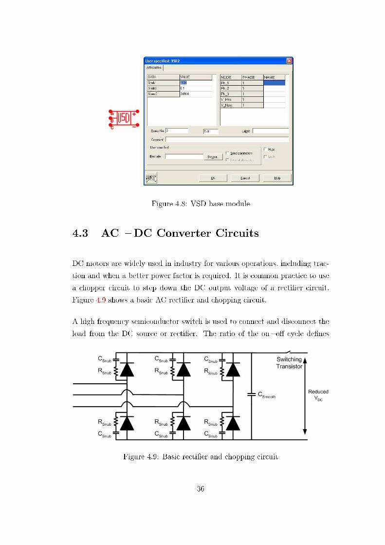
Figure 4.8: VSD base module

4.3 AC {DC Converter Circuits

DC motors are widely used in industry for various operations, including trac-

tion and when a better power factor is required. It is common practice to use

a chopper circuit to step down the DC output voltage of a recti�er circuit.

Figure 4.9 shows a basic AC recti�er and chopping circuit.

A high frequency semiconductor switch is used to connect and disconnect the

load from the DC source or recti�er. The ratio of the on { o� cycle de�nes

Figure 4.9: Basic recti�er and chopping circuit

36

V in

t on t off

Average V out

Actual V out

Figure 4.10: Chopper actual and average output voltage

the average value of the DC voltage received by the load, see Figure 4.10 [25].

If the ratio of switch time { on (ton) to time { o� (to�) is 0.8, then the output

voltage can be de�ned as in Equation 4.1.

Vout = 0:8Vin (4.1)

whereVout = the average DC output voltage of the chopper

Vin = the DC input voltage of the chopper

4.3.1 Basic Model of Chopper

A basic model of the recti�er and chopper circuit was developed as in Fig-

ure 4.9. The load is directly connected across the DC link and so the DC link

does not act as a harmonic �lter, as with the AC{AC converter. Therefore

in the module the machine was represented by its armature impedance and a

back e.m.f. Figure 4.11 shows the equivalent circuit used for the DC machine.

An initial simulation veri�ed that the DC voltage supplied to the load was

the desired average value. The duty cycle and back e.m.f were then varied to

37

Figure 4.11: DC machine equivalent circuit

Figure 4.12: DC armature parameter measurement

obtain the required current. The voltage and current ratings where taken from

actual machines. Measurements do not include brushes as they are nonlinear

elements, measurements were taken using wires inserted between the brushes

and the commutator as shown in Figure 4.12.

4.3.2 Chopper Model Evaluation

A simulation containing both a chopper and load was compiled. The sim-

ulations also included a transformer to con�rm module interaction and that

the results were as expected. Figure 4.13 shows the simulated chopper output

voltage and average output voltage. The simulated load was a 24 kW DC

38

0 1 2 3 4 5 6 7 8x 10−4

0

200

400

600

800

1000

1200

1400

Time (s)

Volta

ge (V

)

Actual VAverage V

Figure 4.13: Simulated chopper output voltage and average voltage

machine of rated voltage 220 V supplied via a basic three phase transformer

(see Section 4.4).

The current drawn was con�rmed in the same manner and a data base module

was created. The module allowed for user de�ned back e.m.f, DC link ca-

pacitance, load resistance, load inductance, snubber capacitance and snubber

resistance.

4.4 Transformer

Transformers are designed to operate below conditions of saturation [5], im-

plying that operation occurs in a linear region. A harmonic evaluation is done

under normal operating conditions, hence saturation is not of great importance

and can be ignored in a basic transformer model for steady { state simulations.

39

\BCTRAN" [18] is a package within ATP which allows users to create a trans-

former model using measured short circuit and open circuit values. ATP also

allows for a three phase transformer to be de�ned, the leakage and magnet-

ising impedances for each phase and the saturation curves can be individually

entered.

It is possible to calculate approximate transformer impedance values using

information given on the name plate and the assumption that the impedance

is equally divided between the HT and LT sides of the transformer equivalent

circuit. These values can then be entered into ATPs three phase transformer

model.

For networks consisting of many \like" transformers (i.e. same manufacturer

and speci�cation), an average leakage impedance should be used to develop a

standard model. The average impedance can be calculated using the inform-

ation given on the single line diagram of the network.

The connection of the transformer will a�ect calculations, a factor ofp3 should

be included if the transformer is not of like connection on both the HT and

LT sides, i.e. star { star or delta { delta. See Appendix A for calculations.

4.4.1 Model Con�rmation

A delta { star transformer will induce a 30 � phase shift between input and

output currents [26]. This phase shift was con�rmed by measuring an input

and an output line current in an ATP simulation of the transformer, Figure 4.14

shows the results of the simulations con�rming the 30 � phase shift.

The step down ratio was also con�rmed using a simple resistive load. The

transformer model was found to work as expected, and a data base module

was created. User options can include leakage impedance values and voltage

ratios.

40

0 100 200 300 400 500 600 700 800

−1

−0.8

−0.6

−0.4

−0.2

0

0.2

0.4

0.6

0.8

1

Degrees ( o )

Norm

alise

d Cu

rrent

HT CurrentLT Current

Figure 4.14: � { � transformer HT and LT line currents

VSD{Transformer Module Interaction

The transformer model will have to be included in the same circuits as the

VSD model and so it is important that the models produce expected results

when used together.

A simple network comprising of a transformer and a VSD was simulated. The

simulation appeared to be sensitive to symmetry resistance (Section 4.2.2)

and the interaction between the VSD module and the transformer module also

caused non-realistic results.

A short transmission line between modules forces ATP to solve the network in

small subsections. This is caused by the propagation time of the transmission

line (a few microseconds for a 1 km line). This delay causes the calculations for

each device to be performed separately preventing undesired (mathematical)

interaction between the modules. The short transmission line does not a�ect

the overall result.

An initial simulation was done with multiple symmetry resistors (decoupling

41

0.018 0.02 0.022 0.024 0.026 0.028 0.03 0.032 0.034 0.036

−1000

−500

0

500

1000

Time (s)

Curre

nt (A

)

Figure 4.15: Simulated LT line current

the modules) in series with the VSD. The results are shown in Figures 4.15

and 4.16. It can be seen from the symmetry of the waveforms that no source

impedance or unbalance has been included in the simulation. The distortion

of the current waveform seams extreme in comparison with a purely sinusoidal

wave, this is because the current drawn is for only one VSD load on the net-

work, without any other impedances. In a fully modelled network other loads

will draw sinusoidal currents, and the current drawn by the VSD will distort

the pure 50 Hz waveform drawn by other equipment.

In a delta { star transformer the primary phase current is the scaled instantan-

eous di�erence between two secondary currents [5], therefore the HT current

waveform, Figure 4.16, can be attributed to the delta-star conversion of the

transformer [26].

With the introduction of source impedance into the model an underling 50 Hz

waveform was found. This result is as expected and in accordance with actual

measurements, which shows other elements to a�ect the overall current drawn

by the system. Figure 4.17 shows the HT line current waveform. The waveform

can be seen to oscillate on a 50 Hz signal.

42

0.015 0.02 0.025 0.03 0.035

−50

−40

−30

−20

−10

0

10

20

30

40

50

Time (s)

Curre

nt (A

)

Figure 4.16: Simulated HT line current

0.125 0.13 0.135 0.14 0.145 0.15

−25

−20

−15

−10

−5

0

5

10

15

20

25

Time (s)

Curre

nt (A

)

Figure 4.17: Simulated HT line current, including source impedance

43

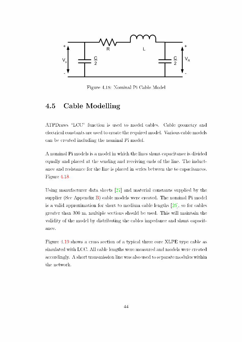
Figure 4.18: Nominal Pi Cable Model

4.5 Cable Modelling

ATPDraws \LCC" function is used to model cables. Cable geometry and

electrical constants are used to create the required model. Various cable models

can be created including the nominal Pi model.

A nominal Pi models is a model in which the lines shunt capacitance is divided

equally and placed at the sending and receiving ends of the line. The induct-

ance and resistance for the line is placed in series between the to capacitances.

Figure 4.18

Using manufacturer data sheets [27] and material constants supplied by the

supplier (See Appendix B) cable models were created. The nominal Pi model

is a valid approximation for short to medium cable lengths [26], so for cables

greater than 300 m, multiple sections should be used. This will maintain the

validity of the model by distributing the cables impedance and shunt capacit-

ance.

Figure 4.19 shows a cross section of a typical three core XLPE type cable as

simulated with LCC. All cable lengths were measured and models were created

accordingly. A short transmission line was also used to separate modules within

the network.

44

Steel Armour

Conductor

XLPE Insulation

PVC Insulation

Figure 4.19: Cable Geometry

4.5.1 Model Con�rmation

Cable models were con�rmed using the transformer module. A network com-

prising a resistive load, transformer and cable was simulated. The transformer

ratio and phase shift (delta { star) were checked. The phase shift did not

change, and the transformer ratio was unchanged. A voltage drop was meas-

ured across long cables. From these simulations the cable models were found

not to interact with other modules.

4.6 Induction Machine Modelling

The induction machine is a common piece of equipment on any industrial net-

work, it is the workhouse of industry. An induction machine equivalent circuit

is shown in Figure 4.20. The ideal transformer in Figure 4.20(a) develops the

rotor e.m.f. The equivalent circuit in Figure 4.20(b) shows the rotor circuit

referred to the stator side, eliminating the ideal transformer. The impedance

values are scaled by the turns ratio of the ideal transformer and the load res-

istance is also scaled by a function of the machine slip.

45

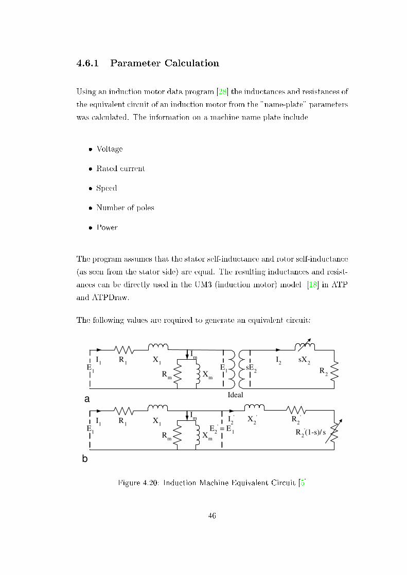
4.6.1 Parameter Calculation

Using an induction motor data program [28] the inductances and resistances of

the equivalent circuit of an induction motor from the "name-plate" parameters

was calculated. The information on a machine name plate include

� Voltage

� Rated current

� Speed

� Number of poles

� Power

The program assumes that the stator self-inductance and rotor self-inductance

(as seen from the stator side) are equal. The resulting inductances and resist-

ances can be directly used in the UM3 (induction motor) model [18] in ATP

and ATPDraw.

The following values are required to generate an equivalent circuit:

I 1 R 1 X 1 I m

R m X m

E 1 sE 2

I 2 sX 2 R 2

Ideal

E 1

I 1 R 1 X 1 I m

R m X m

E 2 ' = E 1

I 2 ' X 2

'

R 2 ' (1-s)/ s E 1

R 2 '

a

b

Figure 4.20: Induction Machine Equivalent Circuit [5]

46

� The nominal phase to phase voltage in kV. It must be greater than

0.005 kV.

� The nominal useful active power in kW, which should be greater than

0.001kW. It is assumed that the power consumed in the �ctitious resist-

ance R2'(1�s)s

of the equivalent circuit is the same as the nominal power.

� The slip at nominal voltage and power. Slip is limited between 0.001 and

0:5.

� The electrical e�ciency at nominal voltage and power. It must be smaller

than 1 and larger than 0:5.

� Power factor (or cos �) at nominal voltage and power. It must be larger

than 0.5 and smaller than 0.999.

� Ratio of locked rotor current (or starting current) and nominal current.

Typically between six and nine.

The program interface is shown in Figure 4.21. Typical e�ciencies and power

factors [29, 30] were used to calculate various induction machine models.

4.7 Conclusion

The individual pieces of equipment modelled in this chapter were veri�ed

through comparison with actual measurements of equipment. Therefore, they

are suitable for use in a simulation of a complete network.

The models created are not an exhaustive list, but the process followed can be

used to create additional models required for future studies. Namely, the use

of equivalent ciruits as the basic model, simpli�cation and comparison with

actual results.

The study conducted in Section 5.4 is of network which comprises each of the

machines discussed previously, and so the models will be used for the study.

47

Figure 4.21: Induction Motor Data Program Interface

48

Chapter 5

Network Analysis

In order to rapidly evaluate the harmonic state of a network, an NRS 048

type study can be performed on the network PCC with the supplier [2]. The

results of such a study will indicate whether or not the network and supply

are operating within harmonic limits.

The assessed state of the PCC can be used to determine possible implications

of alteration or enlargement of the network; this includes the installation and

removal of equipment.

This chapter discusses the approach taken to perform a study and evaluate a

network using an NRS 048 type study and an ATP simulation. Measurement

device selection and data processing methods are also discussed.

5.1 Brandspruit Colliery

Brandspruit Colliery is one of the �ve coal mines operated by SASOL mining

at Secunda. The coal seam is approximately 170 m below surface. The retic-

ulation network is an 11 kV three phase feed to the underground operations.

The network is continually changing as the mining faces move further from the

shaft.

49

5.1.1 Plant Description

Multiple transformers are used to supply power underground. The network

is con�gured so that it can be operated from any combination of the trans-

formers, through the use of ring feeds. This feature allows the sections of

the network to be switched o� for maintenance and expansions, while also

providing redundancy in case of break down. It is also therefore possible to

group similar equipment on the same transformer and so minimise harmonic

interference to other equipment.

The conveyor belt system is driven by VSDs, manufactured by A.B.B., with

belts starting in each working section. Section belts pass coal onto the main

belts, which in turn transfer it to the incline belts which take it to SASOL

Coal Supply.

At various strategic points, underground, substations are used to house trans-

formers, VSDs, telemetric systems and other electric panels. Typically the

voltage is stepped down to 1.1 kV except for VSD supply, which is 400 V.

Each section is supplied from a transformer which is moved with section. The

1.1 kV supplied to the section is typically used to supply the production equip-

ment shown in Table 5.1.

Table 5.1: Typical section production equipment

Three shuttle cars Two roofbolters

Six jet fans One force fan

One conveyor motor One continuous miner

One pump One feeder breaker

5.1.2 Expansions and Alterations

The number of mining sections is dependant on equipment availability, mar-

ket demand and the coal distribution. Sections will cease to operate during

50

moving, when only machine traction and pumps are operated continuously to

move the machine from one area to another.

As the mining operations expand the need for additional underground substa-

tions, conveyors extensions and additional lighting will a�ect the performance

and operation of the network. Alterations are determined well in advance by

engineering services.

5.2 Resonance Pre { Study

Before commencing a physical study, the author evaluated the network to

determine the resonant frequency at various points of concern. Capacitance

and inductance within the network will interact as described in Section 2.2.1.

The frequency at which a capacitance and inductance will resonate is determ-

ined using Equation 5.1

FR =1

2�pLC

(5.1)

Each substation was simpli�ed to a basic inductive and resistive circuit. The

network was reduced until only busbars which had a capacitive component

were left, all others were combined. This simpli�cation process make a few

assumptions (See Appendix C) which aid calculation, the resonant frequency

is not a hard and fast value, and may vary slightly in practice.

The overall (simpli�ed) inductance value and capacitance value for each re-

maining bus bar was used to determine a resonant frequency.

The network evaluated had two PFC capacitors, one on surface at the main

incomer and a second bank underground, see Figure 5.5.

The resonant frequency at the underground capacitor bank was determined

to be just below the 2nd harmonic, whilst the resonant frequency at the main

51

incomer was determined to be just over the 3rd harmonic. The calculations

are shown in Appendix C.

5.2.1 Implications

The resonant frequencies can be used to determine what harmonic loads would

adversely a�ect the harmonic condition.

When selecting equipment it will be important to minimise the use of loads

which are known to produce harmonics at the resonant frequency. The current

signature of any machine can be easily determined by performing a Fourier

analysis of the machines current input.

The resonant frequency can also be used to monitor measured and simulated

results, whereby frequencies around resonant value can be noted and suitably

�ltered or prevented.

5.3 NRS 048 Evaluation

A basic study of the Brandspruit mine was performed to understand the im-

plications of an NRS 048 type study. The evaluation investigated the under-

ground supply and did not, however, investigate the quality of supply to o�ce

buildings, which contain many PCs with switch mode power supplies.

5.3.1 Measurement Devices

The cost, size, availability and speci�cation of various measuring devices, which

can be used to perform an NRS 048 study, in uence the choice of device

used for a study. Before selecting a device an inspection of the network and

measurement points should be made. Power supply, storage space and access

are factors which in uence this decision.

52

A study performed in a sub station with easy access to the panels and a 220 V

mains supply could make use of any device. However should the sub station be

remotely located and the availability of 220 V is limited then a more specialised

device will be required.

Special care should be taken to use a suitably rated device. Panel CTs may

have outputs which do not fall with in the ADC measurement range causing

possible inaccurate results because the device will function on or below its

operational limit.

Storage Space

PC based solutions have the advantage of large and cheap storage mediums

enabling the device to measure multiple channels for extended periods of time

unattended. The number of channels monitored will be limited by the ADC

used. The system will however require a constant power supply and will be a

large and bulky device, weighing approximately 15 kg [31].

Specialised devices may use a di�erent storage medium which may be limited,

due to the size of the device housing, board size or cost. These smaller devices

may not be able to monitor multiple channels for extended periods of time

and so the data would have to be copied o� and the device reset at regular

intervals throughout the evaluation period [32].

Power Supply

A stand alone system that does not require external power, will use a battery

pack. This pack will provide power to the device for a limited period after

which it will need to be changed or recharged. During this period the device

will be inactive. This smaller system will however be easier to transport and

install. Battery packs can be changed when data is copied o�, minimising the

down time of the device.

53

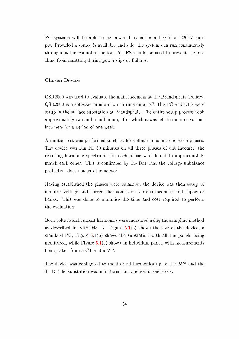
PC systems will be able to be powered by either a 110 V or 220 V sup-

ply. Provided a source is available and safe, the system can run continuously

throughout the evaluation period. A UPS should be used to prevent the ma-

chine from resetting during power dips or failures.

Chosen Device

QSR2000 was used to evaluate the main incomers at the Brandspruit Colliery.

QSR2000 is a software program which runs on a PC. The PC and UPS were

setup in the surface substation at Brandspruit. The entire setup process took

approximately two and a half hours, after which it was left to monitor various

incomers for a period of one week.

An initial test was performed to check for voltage imbalance between phases.

The device was run for 30 minutes on all three phases of one incomer, the

resulting harmonic spectrum's for each phase were found to approximately

match each other. This is con�rmed by the fact that the voltage unbalance

protection does not trip the network.

Having established the phases were balanced, the device was then setup to

monitor voltage and current harmonics on various incomers and capacitor

banks. This was done to minimise the time and cost required to perform

the evaluation.

Both voltage and current harmonics were measured using the sampling method

as described in NRS 048 { 3. Figure 5.1(a) shows the size of the device, a

standard PC, Figure 5.1(b) shows the substation with all the panels being

monitored, while Figure 5.1(c) shows an individual panel, with measurements

being taken from a CT and a VT.

The device was con�gured to monitor all harmonics up to the 25 th and the

THD. The substation was monitored for a period of one week.

54

Figure 5.1: Substation evaluation

55

5.3.2 Data Analysis

QSR2000 has a report generating function, which analyses the data captured in

accordance with NRS 048 version 1. For the authors understanding and future

analysis on data captured on a machine without report writing functionality,

macro code was written to perform the analysis in Microsoft Excel R . This

function was used to generate the voltage harmonic spectrum and THD for the

Brandspruit incomers. The results were found to be within NRS 048 limits,

as shown in Figure 5.2. Appendix D is the macro code written to assess the

recorded data.

An analysis of harmonic current was also performed, the harmonic spectrum

indicated that current harmonics are below maximum levels (overload) ac-

ceptable for capacitor banks. As stipulated in IEC 871 [33, 34], the current

overload for the capacitors is below 30%. Figure 5.3 shows the current har-

monic spectrum.

Although the analysis indicates the network to be operating within harmonic

limits, the continuously varying nature of the network warrants further ana-

lysis. As the network is altered it may cause harmonic situations above the

acceptable limits.

5.3.3 Comments

The measurement process is simple to perform and requires little user input.

The software can be used to evaluate the results in accordance with NRS 048

and clear indication of the harmonic status can be seen.

Using the compatibility levels in Chapter 3 and the results it was con�rmed

that Brandspruit was operating within NRS 048 limits and that there appeared

to be no harmonic problem.

The results, however, do not possess enough detail to draw conclusions as to

the harmonic condition at any point within the network as they do not re ect

56

Figure 5.2: Voltage Harmonic Spectrum of Incomer

Figure 5.3: Measured Current Harmonic Spectrum of Incomer

57

a measurement at points other than the PCC.

The resonant frequency determined in Section 2.2.1 does not feature in the

results of the NRS 048 study. This indicates that loads within the network are

not generating enough 3rd harmonic to cause resonance.

The current results do indicate an elevated 5th harmonic which is caused by

the VSDs used within the network. Figure 4.1 shows the harmonic spectrum

of a typical VSD.

5.4 ATP Simulation

Although the NRS 048 measurements do not indicate an excess of harmonics,

an ATP model of the network was developed and a simulation was conducted

as part of this project. This was used to predict harmonic content throughout

the network. The modelling process is used to help develop steps to complete

a hybrid network evaluation and to allow future alterations to be modelled

before they are commissioned.

An incomer and all of the associated equipment was simulated in ATP. The

devices where simulated as discussed in Chapter 4. Each device of importance

was modelled, and were possible devices were grouped to simplify the total

model. All capacitor banks and individual VSDs were included.

As each new device or substation was added to the network the simulation was

compiled to con�rm that no errors had been included. Although this increased

the development time it prevented a di�cult debugging process of the complete

network model.

58

5.4.1 Problems Encountered

Most errors were created through misinterpretation of the single line diagram

and hence an incorrect model, such as simulating ringfeeds as closed instead of

open. Incomplete information also made the development di�cult and required

many visits to the site to gather extra information.

ATP and ATPDraw are syntax rigid applications that are particular about the

information that is entered. Some errors were created through not following

the exact procedure for creating a model, the ATP Rule book[18] should be

followed when a new model is created.

ATP failed to compile when cables were repeated within the ATPDraw envir-

onment, this occurred when multiple references to the same data base module

were individually created. The problem was overcome by simply copying and

pasting identical elements within the network model. The network diagram is

shown in Figure 5.5.

5.4.2 Simulation Analysis

The completed model was then adjusted to re ect a working example of the

mine's network, including the operation and non-operation of various pieces

of equipment, such as capacitor banks. The result of this simulation was then

compared with the NRS 048 study results.

The NRS 048 results are an indication of the highest value for each harmonic

order, each maximum harmonic value may not occur at the same instant as an-

other harmonics maximum value. The ATP simulation represents a particular

setup and hence a particular set of harmonic values.

In order to best correlate the NRS 048 results and the simulated results the

most signi�cant measured harmonic(s) was selected. The model was then ad-

justed to create a situation where the harmonic value(s) are obtained. The

situation represented a network con�guration which was likely to occur. In

59

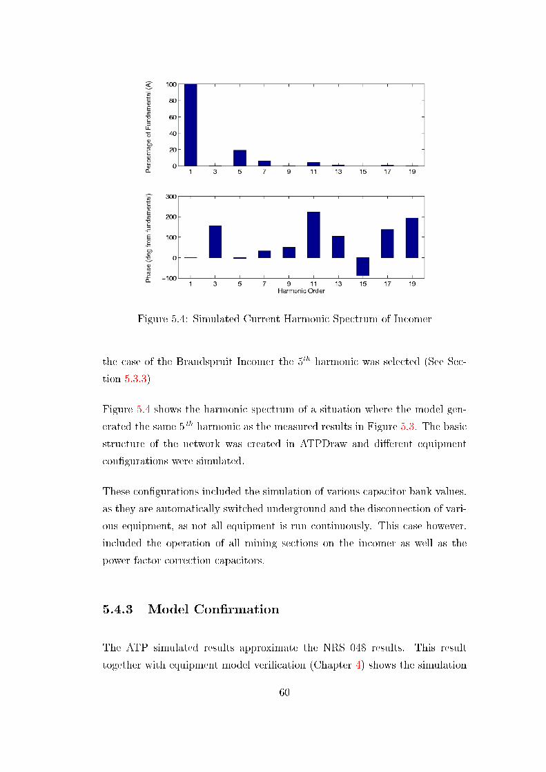
Figure 5.4: Simulated Current Harmonic Spectrum of Incomer

the case of the Brandspruit Incomer the 5th harmonic was selected (See Sec-

tion 5.3.3)

Figure 5.4 shows the harmonic spectrum of a situation where the model gen-

erated the same 5 th harmonic as the measured results in Figure 5.3. The basic

structure of the network was created in ATPDraw and di�erent equipment

con�gurations were simulated.

These con�gurations included the simulation of various capacitor bank values,

as they are automatically switched underground and the disconnection of vari-

ous equipment, as not all equipment is run continuously. This case however,

included the operation of all mining sections on the incomer as well as the

power factor correction capacitors.

5.4.3 Model Con�rmation

The ATP simulated results approximate the NRS 048 results. This result

together with equipment model veri�cation (Chapter 4) shows the simulation

60

methods to be a valid alternative to NRS 048 type evaluations and a additional

tool for harmonic analysis of networks.

5.4.4 Comments

The process to develop an computer model is a long and involved process, this

is due to the need to con�rm each stage of the development of the model,

including individual equipment models.

The process of developing the model is greatly sped up for future studies,

should the equipment models be reusable. The process may be too elaborate

for a one o� case study of a network which is not likely to change.

5.5 Investigation into the Operation of Auto {

Switching Capacitor Banks at Brandspruit

The e�ect of the various operating states of an auto { switching underground

capacitor bank were investigated. The underground capacitor is used for

voltage stability in remote sections of the mine. The amount of power factor

correction required at the point is dependant on the load at the point at any

particular time. A single line diagram of the network is shown in Figure 5.5,

it is one of Brandspruits incomers.

The normal operating state of this capacitor bank (indicated in �gure 5.5),

under these network conditions, is the 1200 kVAr setting. The bank will

automatically switch to give the best power factor, but should one of the

banks be deactivated, for example the 1200 kVAr, a timer prevents it from

being switched back on again for a period of �ve minutes. The concern is that

if a momentary change in network conditions should cause the capacitor bank

to switch o� and then the network conditions return to normal the capacitor

bank may operate outside its speci�ed operating parameters. The overstressing

61

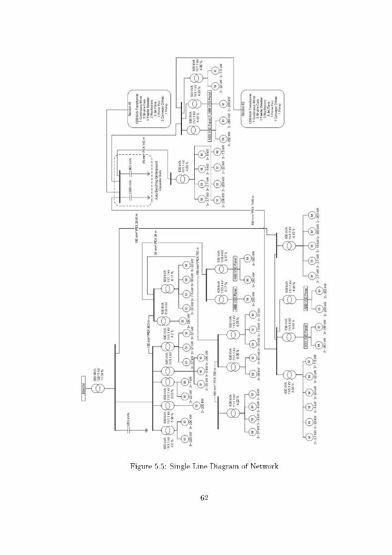
Figure 5.5: Single Line Diagram of Network

62

0 5 10 15 20 25 30 35 400

10

20

30

Abs

mag

nitu

de (A

)

0 5 10 15 20 25 30 35 40−100

0

100

200

300

Phas

e (d

eg fr

om fu

ndam

enta

l)

Harmonic Order

Figure 5.6: Current Harmonic Signature of 600 kVAr Capacitor

of capacitors can cause degradation of dielectrics, overheating and failure of

the capacitor.

The capacitor bank was modelled in three of its settings, namely 600 kVAr,

1200 kVAr and 1800 kVAr. The rest of the network was held constant for the

three simulations. Figures 5.6, 5.7 and 5.8 show the harmonic spectrum of

the current drawn by the underground capacitor bank. From Figure 5.7 the

current THD can be calculated to be 9:19%.

The same calculations were performed for each of the other simulations (dif-

ferent capacitor bank settings), the results of which are shown in Table 5.2.

The table also includes the THD, rated r.m.s current, the r.m.s value of the

simulated waveform and the percentage over current.

In all three cases the capacitor bank is operated below a 30% over current

and so the opeating characteristics are suitable and the capacitor bank is not

operated in a dangerous manner.

It should however be noted that the if the capacitor bank is manually operated

63

1 3 5 7 9 11 13 15 17 190

20

40

60

Abs

mag

nitu

de (A

)

1 3 5 7 9 11 13 15 17 19−100

0

100

200

Phas

e (d

eg fr

om fu

ndam

enta

l)

Harmonic Order

Figure 5.7: Current Harmonic Signature of 1200 kVAr Capacitor

1 3 5 7 9 11 13 15 17 190

20

40

60

80

Abs

mag

nitu

de (A

)

1 3 5 7 9 11 13 15 17 19−100

−50

0

50

100

150

Phas

e (d

eg fr

om fu

ndam

enta

l)

Harmonic Order

Figure 5.8: Current Harmonic Signature of 1800 kVAr Capacitor

64

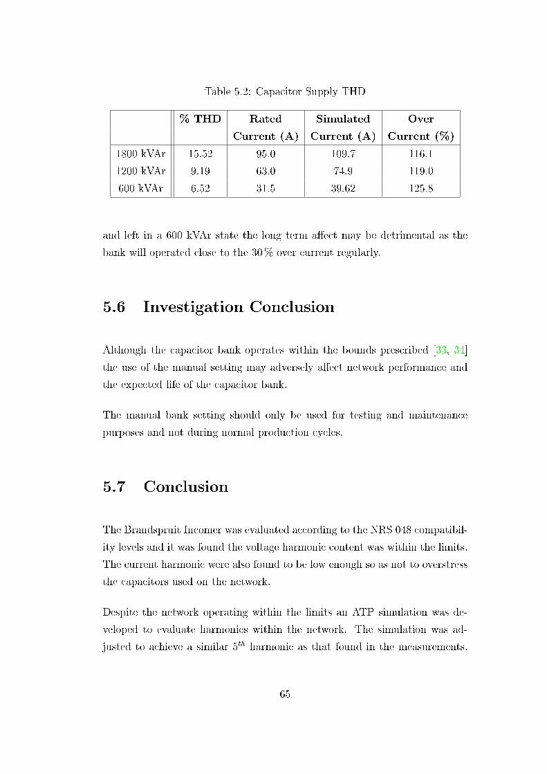
Table 5.2: Capacitor Supply THD

% THD Rated Simulated Over

Current (A) Current (A) Current (%)

1800 kVAr 15.52 95.0 109.7 116.1

1200 kVAr 9.19 63.0 74.9 119.0

600 kVAr 6.52 31.5 39.62 125.8

and left in a 600 kVAr state the long term a�ect may be detrimental as the

bank will operated close to the 30% over current regularly.

5.6 Investigation Conclusion

Although the capacitor bank operates within the bounds prescribed [33, 34]

the use of the manual setting may adversely a�ect network performance and

the expected life of the capacitor bank.

The manual bank setting should only be used for testing and maintenance

purposes and not during normal production cycles.

5.7 Conclusion

The Brandspruit Incomer was evaluated according to the NRS 048 compatibil-

ity levels and it was found the voltage harmonic content was within the limits.

The current harmonic were also found to be low enough so as not to overstress

the capacitors used on the network.

Despite the network operating within the limits an ATP simulation was de-

veloped to evaluate harmonics within the network. The simulation was ad-

justed to achieve a similar 5th harmonic as that found in the measurements.

65

The model was then used to investigate the operation of auto { switching ca-

pacitor banks underground. Recommendations were made as to the use of the

auto { switching capacitor.

The chapter con�rmed that both measurement and simulation could be suc-

cessfully used to investigate the harmonic condition of an electrical network.

66

Chapter 6

Hybrid Evaluation

Although both an NRS 048 study and a simulation could be used to evaluate

a network, a hybrid method making use of both methods strong points can

be used. While an NRS 048 study is quick and relatively easy to perform

it is focused on evaluating the quality of supply as apposed to investigating

problems within a customers network.

On the other hand a computer simulation is a very theoretical approach and

may not fully capture the complexity of the network. The model's integrity

relies on the person whom developed it and his/her assumptions, as well as

the software used.

In order to best use the tools and methods available for a study, a hybrid

approach was developed making use of the best features of both methods.

6.1 Initial Analysis

The �rst step in a harmonic evaluation is to establish if there is in fact a

harmonic condition which is of concern or if future additions and modi�cations

will cause such a harmonic condition. The simplest and quickest method to

achieve such an understanding of the network in question is to perform an

abridged NRS 048 study over a full working day or two.

67

Comparing measured results with NRS 048 limits (see Chapter 3) it can be

determined whether the network operates within acceptable limits and whether

the cause is equipment within the client network or pollution from the national

grid [2]. Should the results con�rm there to be no cause for concern and no

future \harmonic { creating" expansions or modi�cations are expected then no

further investigation is required.

However should the results demonstrate that there is in fact a harmonic prob-

lem or there are \harmonic { creating" expansions or modi�cations planned for

the future, a computer simulation may prove to be necessary to fully under-

stand the problem and evaluate future expansions and modi�cations.

6.2 Network Modelling

Should a model be deemed necessary a complete single line diagram of the net-

work should be acquired and veri�ed. Models of individual pieces of equipment

should be created and veri�ed, as in Chapter 4.

The individual equipment models can then be used to simulate an entire net-

work. The method described in Section 5.4.2 should be used to con�rm the

validity of the plant model.

Once the model has been con�rmed it can be used to evaluate nodes within the

network. Points of concern can be determined by regular faults and failures

of equipment or nuisance tripping within the network. These records should

be kept by the condition monitoring department and a report of regular faults

can be drawn. The supply quality to power factor correction capacitors and

other harmonic sensitive devices should be simulated.

Figure 6.1 shows the simulated harmonic spectrum of the current supplied to

a PFC capacitor, the harmonic values are represented as a percentage of the

fundamental current. The total harmonic distortion is below 30% and so the

capacitor is operating within accepted limits [33, 34].

68

0

20

40

60

80

100

Perc

enta

ge o

f Fun

dam

enta

l (A)

1 3 5 7 9 11 13 15 17 19−300

−200

−100

0

100

Phas

e ( o fr

om fu

ndam

enta

l)

Harmonic Order

Figure 6.1: Current Supplied to Power Factor Correction Capacitor

ATP can be used to simulate the supplied voltage and current to the nodes of

interest. This is far more convenient than having to travel to the node, disrupt-

ing operations to connect and then again to disconnect measuring equipment.

The results of the simulation can be used to determine and evaluate the ap-

propriate solution to the problem, whether it be a recon�guration of network

connections, alteration of transformer connections or the introduction of har-

monic �lters. The proposed solution can be simulated and its e�ect on the

overall harmonic content of the network quanti�ed.

6.3 Conclusion

The quick physical study of the network establishes the overall harmonic con-

dition of the network, giving an indication of whether or not further investig-

ation is required. The abridged study is a clear indication and although not a

complete study in terms of NRS 048 it is su�cient.

69

The modelling process gives an insight into the network making it possible

to evaluate speci�c nodes within the network. The initial model setup can

be time consuming to establish and so modelling should only be performed if

there is a proper justi�cation for it.

Newer software packages make use of gui's and are typically shipped with a

large selection of standardised models [21]. It is possible to establish a network

model quicker using a newer package, but the cost of the software and hardware

required may become prohibitive.

This hybrid approach allows the study to be as complex or as simple as re-

quired. A brief NRS 048 study allows the harmonics to be rapidly evaluated,

whilst an in depth simulation creates a forum for a thorough investigation and

evaluation of solutions without raising equipment costs or disrupting produc-

tion.

70

Chapter 7

Conclusion

The project successfully demonstrated that a combination of measurements

and simulations could be used to thoroughly investigate the harmonic state of

a network.

An NRS 048 study of the Brandspruit network, using a QSR2000 PC based

solution, revealed that Brandspruit was operating within harmonic limits.

Both the voltage and current harmonics were measured.

For the purposes of this project and the future use by Brandspruit an ATP

model was created and a simulation performed. The simulation also indicated

that Brandspruit currently operates within NRS 048 limits.

Individual ATP models for equipment used in the mine, including VSDs, trans-

formers, cables and induction machines, were created and tested. The assump-

tions made in order to develop the model were discussed and wherever possible

models were simpli�ed to decrease processing time. This process helped build

a repository of models which can be used for rapid development of network

models in the future. The use of previously created models decreases the time

required to develop a working model of a plant's network.

The methods and results used for these two individual approaches were used

to suggest a future method which used aspects from both. The simulation is

only created if needed and is con�rmed via the measurements taken. NRS 048

71

limits [2] and IEC 871 [33, 34] speci�cations are used to decide whether or not

the network is operating outside of harmonic limits.

The process allows for a more rapid and unobtrusive harmonic evaluation. The

measurements can be taken at surface substations quickly, without disrupting

production. A computer simulation of the network can then be created and

compared to measurements taken. The simulation can then be con�gured to

include all proposed corrections and hence evaluate them before implementa-

tion.

An evaluation of an underground capacitor bank revealed that the autoswitch-

ing system was suitably con�gured and it also indicated that the use of manual

settings was not advisable as prolonged use may damage equipment.

72

References

[1] J. Arrillaga, D.A. Bradley, and P.S. Bodger. Power Sytem Harmonics.

John Wiley & Sons, New York, 1985.

[2] NRS. Procedures for measuremnt and reporting, NRS 048-3 (Electricity

Supply - Quality of Supply). NRS, 1998.

[3] J. Arrillarga and N.R. Watson. Power System Harmonics. John Wiley &

Sons, Ltd, Chichester, 2nd edition, 2003.

[4] S.A. Nasar. Electric Energy Systems. Prentice Hall, Inc, New Jersey,

1996.

[5] M.G. SAY. Alternating Current Machines. Pitman Publishing Limited,

London, 5th edition, 1984.

[6] M.G. SAY. The Performance and Design of Alternating Current Ma-

chines. Sir Isaac Pitman & Sons LTD, London, 3rd edition, 1968.

[7] Collaboration. The Collaborative International Dictionary of English

v.0.48. dict.org:2628. Last accessed 6 December 2005.

[8] J. Van Coller. Harmonics in Power Systems { An Introduction. University

of the Witwatersrand, School of Electrical and Information Engineering,

May 2002.

[9] Guide To The Application Of Engineering Recommendation G5/4 - In

The Assessment Of Harmonic Voltage Distortion And Connection Of

Non-Linear Equipment To The Electricity Supply System In The Uk. Elec-

tricity Association Services Limited, 2002.

73

[10] GAMBICA Members. Managing Harmonics - A guide to EA Engineering

Recommendation G5/4. http://www.gambica.org.uk/newsite/pdfs/G54{

2.pdf, 2003. Last accessed 12 Nov 2003.

[11] NRS. Overview of implementation of standards and procedures, NRS 048-1

(Electricity Supply - Quality of Supply). NRS, 1996.

[12] NRS. Minimum standards, NRS 048-2 (Electricity Supply - Quality of

Supply). NRS, 1996.

[13] NRS. Application guidlines for utilites, NRS 048-4 (Electricity Supply -

Quality of Supply). NRS, 1999.

[14] NRS. Instrumentation and transducers for voltage quality monitoring and

recording, NRS 048-5 (Electricity Supply - Quality of Supply). NRS, 1998.

[15] J. Wood. Harmonics in power systems. Technical report, RWW Engin-

eering (Pty) Ltd, 2002.

[16] G. Wakileh. Power System Harmonics: Fundamentals, Analysis and Fil-

ter Design. Springer, Berlin, 2001.

[17] S.R.W Egner and J. Van Coller. Guidelines for computer simulation to

supplement measurements of harmonic levels in a reticulation network.

In South African Universities Power Engineering Conference Proceedings,

page Paper F1B1. SAIEE, 2003.

[18] Leuven EMTP Centre. Alternative Transients Program Rule Book. Leuven

, Belgium, 1992.

[19] H. K. H�idalen. ATPDraw. SINTEF Energy Reasearch, Norway, 2002.

[20] The Mathworks Inc. MATLAB with Simulink Power System Toolbox,

version 6.5.0.180913a. 2002.

[21] DIgSILENT GmbH. DIgSILENT PowerFactory 12.1.194a. Gomaringen,

Germany, 2002.

[22] P. Vas. Vector Control of AC Machines. Oxford University Press, Oxford,

1990.

74

[23] W. Xu, H. W. Dommel, M. B. Hughes, G. W. K. Chang, and L. Tan.

Modelling of adjustable speed drives for power system harmonic analysis.

IEEE Transactions on Power Delivery, 14:595 { 601, 1999.

[24] J. Van Coller. Personal Communication. University of the Witwatersrand,

School of Electrical Engineering, Johannesburg, 2003.

[25] A. Kusko. Solid-State DC Motor Drives. The M.I.T Press, Cambridge,

Massachusetts, 1969.

[26] J.J. Grainger and W.D. Stevenson. Power System Analysis. McGraw-Hill,

New York, 1994.

[27] Aberdare Cables (Pty) Limited. Three Core Cable Data Sheets. Aberdare

Cables (Pty) Limited, 2003.

[28] I. Leikkonen. Induction Motor Data Program.

http://pp.kpnet.�/ijl/prog.htm, December 2004.

[29] ABB. DriveIT Low Voltage Cast Iron Motors. M2000 Range.

http://www.abb.com. Last accessed 9 December 2003.

[30] ABB. M3000 Steel Motors. ABB LV M3000 Range. http://www.abb.com.

Last accessed 9 December 2003.

[31] TLC Software. TLC Software Products.

http://www.tlc.co.za/products.htm. Last accessed 26 Nov 2002.

[32] CT Lab. Vectograph. http://www.ctlab.co.za. Last accessed 10 December

2003.

[33] IEC. General { Performance, testing and rating { Safety requirements {

Guide for instulation and operation, IEC 60871 { 1 (Shunt Capacitors for

a.c. power systems having a rated voltage above 1000 V). IEC, 1997.

[34] IEC. Endurance tesing, IEC TS 60871 { 2 (Shunt Capacitors for a.c. power

systems having a rated voltage above 1000 V). IEC, 1999.

75

Appendix A

Transformer Model Calculations

A delta { star connected transformer can be approximated by three single phase

transformers connected as a star on the primary side and a delta on the sec-

ondary side.

Each individual transformer can then be modelled, the transformer ratio will

be given by

a =Vp

Vs=p3

whereVp = Primary line voltage

Vs = Secondary line voltage

a = transformer turns ratio

Let

Vb = Vp

kVAb = kVAT=3

wherekVAT = Three phase kVA rating

kVAb = kVA base

Therefore

Ib = kVAb=Vb

Zb = Vb=Ib

76

whereVb = Voltage base

Ib = Current base

Zb = Impedance base

Using the percentage leakage impedance value for the transformer the actual

leakage impedance can be found as follows

Zl = Z% � Zb

whereZ% = Percentage leakage impedance

Zl = Leakage impedance value

Assuming that the impedance is equally split between the HT and LT side the

values of the transformer equivalent circuit can be found

Zp =Zl

2

Zs =Zl

2a2

whereZp = Primary impedance

Zs = Secondary impedance

The primary resistance and inductance and secondary resistance and induct-

ance can then be determined and used in the ATP three phase transformer

model.

77

Appendix B

Cable Data

As per telephonic conversation with Adriaan Klark of Aberdare Cables (Pty)

Limited, Port Elizabeth. The follow cable coe�cients were con�rmed.

Cable armour resistivity is 4:52� 10�7 m

Relative permeability of pipe conductor is 400

Relative permittivity of PVC insulation is 8

Relative permittivity of XLPE insulation is 2:5

Conductor resistivity is 1:7� 10�8 m

78

Appendix C

Resonance Calculations

The resonant frequecy at each of the two capcitor banks, on the Brandspruit

network that was investigated, was determined. Initially all machines were

accounted for and then the network was reduced to single capacitance, induct-

ance and resistance connected to each of the two bus bars.

C.1 Machine Equivalent Circuits

The �rst step was to calculate an equivalent resistance and inductance for each

type of machine. This included various induction machines and transformers.

The results are discussed below.

C.1.1 Induction Motors

Figure C.1 shows the basic equivalent circuit of an induction machine, as used

by the induction motor parameter program [28]. RL in the induction machine

model is equal to R02(1�s)s

.

The induction motor program was used to generate the equivalent circuit val-

ues, and these values were reduced to �nd the overall impedance of the machine

at a particular slip. The equivalent circuit values for the various machines are

79

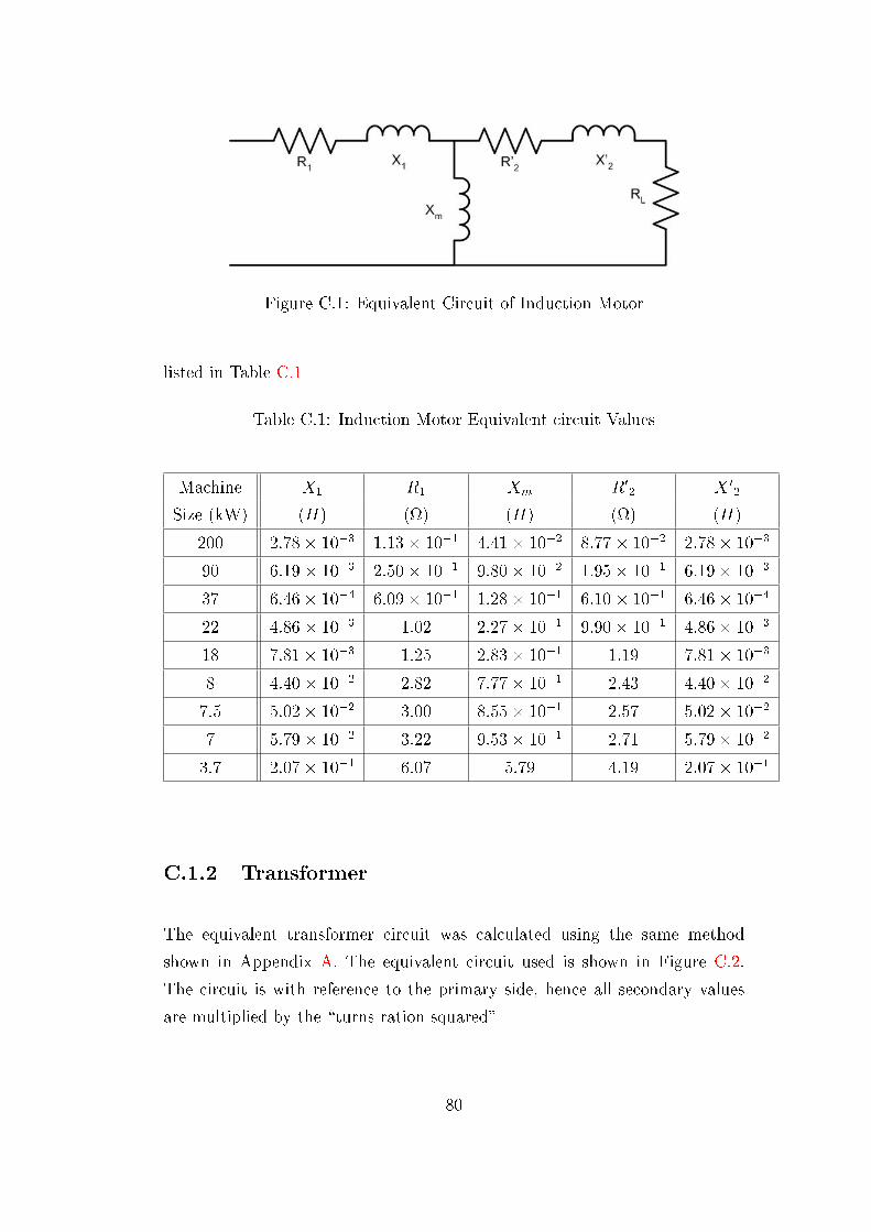
Figure C.1: Equivalent Circuit of Induction Motor

listed in Table C.1

Table C.1: Induction Motor Equivalent circuit Values

Machine X1 R1 Xm R02 X 02

Size (kW) (H) () (H) () (H)

200 2:78� 10�3 1:13� 10�1 4:41� 10�2 8:77� 10�2 2:78� 10�3

90 6:19� 10�3 2:50� 10�1 9:80� 10�2 1:95� 10�1 6:19� 10�3

37 6:46� 10�4 6:09� 10�1 1:28� 10�1 6:10� 10�1 6:46� 10�4

22 4:86� 10�3 1:02 2:27� 10�1 9:90� 10�1 4:86� 10�3

18 7:81� 10�3 1:25 2:83� 10�1 1:19 7:81� 10�3

8 4:40� 10�2 2:82 7:77� 10�1 2:43 4:40� 10�2

7.5 5:02� 10�2 3:00 8:55� 10�1 2:57 5:02� 10�2

7 5:79� 10�2 3:22 9:53� 10�1 2:71 5:79� 10�2

3.7 2:07� 10�1 6:07 5:79 4:19 2:07� 10�1

C.1.2 Transformer

The equivalent transformer circuit was calculated using the same method

shown in Appendix A. The equivalent circuit used is shown in Figure C.2.

The circuit is with reference to the primary side, hence all secondary values

are multiplied by the \turns ration squared"

80

Figure C.2: Equivalent Circuit of a Transformer

Conclusion

The equivalent circuits for the machines were calculated and reduced assuming

a slip of 0.95 [29, 30]. This is an assumption of the loading of a machine

and does not cover all operating conditions for each machine. It is a suitable

approximation as it assumes a typical operating load and is very likely to occur

during production.

C.2 Network Reduction

The reduced machine circuits were grouped together to form the network as

show in in Figure 5.5. The bus bars were grouped so that all inductive and

resistive loads downstream of a bus bar, with capacitance, were combined. The

following �gures (C.3 to C.8) show the reduction of each individual bus bar to

single impedance value.

The individual impedance value of each bus bar was then used to reduce the

network to a single impedance (inductive and resistive) value, as shown in

Figure C.9. This imductance together with the capacitive value was used to

calculate the expected resonant frequency at the bus bar.

81

Figure C.3: Bus Bar 1 Reduction

Figure C.4: Bus Bar 2 Reduction

82

Figure C.5: Bus Bar 3 Reduction

Figure C.6: Bus Bar 4 Reduction

Figure C.7: Bus Bar 5 Reduction

83

Figure C.8: Bus Bar 6 Reduction

Figure C.9: Reduced Circuit for Calculation of Resonant Frequency at Surface

PFC

84

From the impedance value the inductance was calculated in the following man-

ner L = X2�f

= 23:78mH and therefore the resonant frequency was found as

follows

f = 12�pLC

= 1

2�p

31:57�F�23:78mH= 183:69Hz

The resonant frequency is between harmonics (between 3rd and 4th) and hence

is unlikely to be of concern.

The resonant frequency as calaculated in the same manner as above and was

found to be nearly the 2nd harmonic. resonance is unlicely to occur as there

are no harmonic sources which produce a signi�cant amount of 2nd harmonic.

85

Appendix D

Excel Macro Code

This �rst code copies and seperates the data to di�erent worksheets.

Sub column_copy()

Dim counter As Integer

Dim Junk As Integer

Dim sheetcount As Integer

Sheets.Add Count:=4

Sheets(4).Name = ("A %Fund")

Sheets(3).Name = ("A %RMS")

Sheets(2).Name = ("V %Fund")

Sheets(1).Name = ("V %RMS")

For sheetcount = 1 To 4

'Copies the time Column

Sheets(5).Select

Columns(3).Select

Selection.Copy

Sheets(sheetcount).Select

Cells(1, 1).Select

ActiveSheet.Paste

'Copies respective THD Coloumn

Sheets(5).Select

86

Columns(9 + sheetcount).Select

Selection.Copy

Sheets(sheetcount).Select

Cells(1, 3).Select

ActiveSheet.Paste

'Copies Individual Harmonics

For counter = 0 To 15

Junk = counter * 4

Sheets(5).Select

Columns(16 + sheetcount + Junk).Select

Selection.Copy

Sheets(sheetcount).Select

Cells(1, counter + 4).Select

ActiveSheet.Paste

Next counter

Next sheetcount

End Sub

This code determines the 95% value, as per NRS 048 .

Sub stat_check()

Dim colcount, rowcount, rowcounter As Integer

Dim comval As Single

Dim cellform As String

For sheetcount = 1 To 4

'select sheet to be edited

Sheets(sheetcount).Select

'start at the cell "A1"

rowcount = 1

colcount = 1

'Count the number of rows

While Cells(rowcount, colcount).Value <> ""

rowcount = rowcount + 1

Wend

'set Headings

Cells(rowcount + 1, 1).Value = "Mean"

87

Cells(rowcount + 2, 1).Value = "Standard Dev"

Cells(rowcount + 3, 1).Value = "Valid Min"

Cells(rowcount + 4, 1).Value = "Valid Max"

Cells(rowcount + 5, 1).Value = "Measured Max"

'Set up mean, standard Devation and max and min valid values

For colcount = 3 To 19

cellform = "=average(r[-" & rowcount - 1 & "]c:R[-2]c)"

Cells(rowcount + 1, colcount).FormulaR1C1 = cellform

cellform = "=stdev(r[-" & rowcount & "]c:R[-3]c)"

Cells(rowcount + 2, colcount).FormulaR1C1 = cellform

comval = Cells(rowcount + 2, colcount)

Cells(rowcount + 2, colcount) = comval

Cells(rowcount + 3, colcount).FormulaR1C1 = "=R[-2]C - R[-1]c"

comval = Cells(rowcount + 3, colcount)

Cells(rowcount + 3, colcount) = comval

Cells(rowcount + 4, colcount).FormulaR1C1 = "=R[-3]C + R[-2]c"

comval = Cells(rowcount + 4, colcount)

Cells(rowcount + 4, colcount) = comval

cellform = "=max(r[-" & rowcount + 4 & "]c:R[-6]c)"

Cells(rowcount + 5, colcount).FormulaR1C1 = cellform

comval = Cells(rowcount + 5, colcount)

Cells(rowcount + 5, colcount) = comval

Next colcount

'Make statistically irrelivant data red

For colcount = 3 To 19

For rowcounter = 2 To rowcount

If Cells(rowcounter, colcount).Value < Cells(rowcount + 3, colcount) Then

Cells(rowcounter, colcount).Font.ColorIndex = 3

End If

Next rowcounter

comval = Cells(rowcount + 4, colcount)

For rowcounter = 2 To rowcount

If Cells(rowcounter, colcount).Value > Cells(rowcount + 4, colcount) Then

88

Cells(rowcounter, colcount).Font.ColorIndex = 3

End If

Next rowcounter

Next colcount

Next sheetcount

End Sub

Run the various functions in order and saves the �les.

Sub workall()

Application.CutCopyMode = False

Application.Run "'macro file.xls'!column_copy"

Application.Run "'macro file.xls'!stat_check"

Application.Run "'macro file.xls'!graphing"

Application.Run "'macro file.xls'!save"

End Sub

Sub save()

Dim strCaption As String

strCaption = Application.Caption

Mid(strCaption, 1, 18) = " "

strCaption = Application.ActiveWorkbook.Path & "\" & Trim(strCaption) & ".xls"

ActiveWorkbook.SaveAs FileName:=strCaption, _

FileFormat:=xlNormal, password:="", Writerespassword:="", _

ReadOnlyRecommended:=False, CreateBackup:=False

End Sub

Plots the graphs

Sub graphing()

Dim rowcount, Count As Integer

Dim strCaption As String

strCaption = Application.Caption

Mid(strCaption, 1, 18) = " "

strCaption = Trim(strCaption)

'---------V % RMS -----------------------------

'Start in the first row

rowcount = 1

'V % RMS

89

Sheets("V %RMS").Select

'need to find the mean row

While Cells(rowcount, 1).Value <> "Mean"

rowcount = rowcount + 1

Wend

'Create better Titles

With ActiveChart

For Count = 0 To 15

Cells(1, Count + 4).Value = 2 * Count + 1

Next Count

End With

'add the chart

Charts.Add

ActiveChart.ChartType = xlColumnClustered

'edit here

With Sheets("V %RMS")

ActiveChart.SetSourceData Source:=.Range("A24:A27"), PlotBy _

:=xlColumns

ActiveChart.SeriesCollection(1).Delete

ActiveChart.SeriesCollection.NewSeries

ActiveChart.SeriesCollection(1).XValues = .Range(.Cells(1, 5), .Cells(1, 19))

ActiveChart.SeriesCollection(1).Values = .Range(.Cells(rowcount, 5), .Cells(rowcount, 19))

ActiveChart.SeriesCollection.NewSeries

ActiveChart.SeriesCollection(2).XValues = .Range(.Cells(1, 5), .Cells(1, 19))

ActiveChart.SeriesCollection(2).Values = .Range(.Cells(rowcount + 3, 5), .Cells(rowcount + 3, 19))

ActiveChart.SeriesCollection.NewSeries

ActiveChart.SeriesCollection(3).XValues = .Range(.Cells(1, 5), .Cells(1, 19))

ActiveChart.SeriesCollection(3).Values = .Range(.Cells(rowcount + 4, 5), .Cells(rowcount + 4, 19))

End With

ActiveChart.Location Where:=xlLocationAsNewSheet, Name:="V % of RMS"

With ActiveChart

.HasTitle = True

.ChartTitle.Text = strCaption

.Axes(xlCategory, xlPrimary).HasTitle = True

'and here

.Axes(xlCategory, xlPrimary).AxisTitle.Characters.Text = "Harmonic Order"

.Axes(xlValue, xlPrimary).HasTitle = True

.Axes(xlValue, xlPrimary).AxisTitle.Characters.Text = "% V of RMS V"

End With

With ActiveChart.Axes(xlCategory)

.HasMajorGridlines = False

.HasMinorGridlines = False

End With

With ActiveChart.Axes(xlValue)

.HasMajorGridlines = False

.HasMinorGridlines = False

End With

ActiveChart.HasLegend = False

ActiveChart.HasDataTable = False

90

ActiveChart.PlotArea.Select

Selection.ClearFormats

'---------V %Fund -----------------------------

'Start in the first row

rowcount = 1

Sheets("V %Fund").Select

'need to find the mean row

While Cells(rowcount, 1).Value <> "Mean"

rowcount = rowcount + 1

Wend

'Create better Titles

With ActiveChart

For Count = 0 To 15

Cells(1, Count + 4).Value = 2 * Count + 1

Next Count

End With

'add the chart

Charts.Add

ActiveChart.ChartType = xlColumnClustered

'edit here

With Sheets("V %Fund")

ActiveChart.SetSourceData Source:=.Range("A24:A27"), PlotBy _

:=xlColumns

ActiveChart.SeriesCollection(1).Delete

ActiveChart.SeriesCollection.NewSeries

ActiveChart.SeriesCollection(1).XValues = .Range(.Cells(1, 5), .Cells(1, 19))

ActiveChart.SeriesCollection(1).Values = .Range(.Cells(rowcount, 5), .Cells(rowcount, 19))

ActiveChart.SeriesCollection.NewSeries

ActiveChart.SeriesCollection(2).XValues = .Range(.Cells(1, 5), .Cells(1, 19))

ActiveChart.SeriesCollection(2).Values = .Range(.Cells(rowcount + 3, 5), .Cells(rowcount + 3, 19))

ActiveChart.SeriesCollection.NewSeries

ActiveChart.SeriesCollection(3).XValues = .Range(.Cells(1, 5), .Cells(1, 19))

ActiveChart.SeriesCollection(3).Values = .Range(.Cells(rowcount + 4, 5), .Cells(rowcount + 4, 19))

End With

ActiveChart.Location Where:=xlLocationAsNewSheet, Name:="V % of Fundamental"

With ActiveChart

.HasTitle = True

.ChartTitle.Text = strCaption

.Axes(xlCategory, xlPrimary).HasTitle = True

.Axes(xlCategory, xlPrimary).AxisTitle.Characters.Text = "Harmonic Order"

.Axes(xlValue, xlPrimary).HasTitle = True

.Axes(xlValue, xlPrimary).AxisTitle.Characters.Text = "% V of Fundamental V"

End With

With ActiveChart.Axes(xlCategory)

.HasMajorGridlines = False

.HasMinorGridlines = False

End With

With ActiveChart.Axes(xlValue)

.HasMajorGridlines = False

91

.HasMinorGridlines = False

End With

ActiveChart.HasLegend = False

ActiveChart.HasDataTable = False

ActiveChart.PlotArea.Select

Selection.ClearFormats

'---------A % RMS -----------------------------

'Start in the first row

rowcount = 1

Sheets("A %RMS").Select

'need to find the mean row

While Cells(rowcount, 1).Value <> "Mean"

rowcount = rowcount + 1

Wend

'Create better Titles

With ActiveChart

For Count = 0 To 15

Cells(1, Count + 4).Value = 2 * Count + 1

Next Count

End With

'add the chart

Charts.Add

ActiveChart.ChartType = xlColumnClustered

'edit here

With Sheets("A %RMS")

ActiveChart.SetSourceData Source:=.Range("A24:A27"), PlotBy _

:=xlColumns

ActiveChart.SeriesCollection(1).Delete

ActiveChart.SeriesCollection.NewSeries

ActiveChart.SeriesCollection(1).XValues = .Range(.Cells(1, 5), .Cells(1, 19))

ActiveChart.SeriesCollection(1).Values = .Range(.Cells(rowcount, 5), .Cells(rowcount, 19))

ActiveChart.SeriesCollection.NewSeries

ActiveChart.SeriesCollection(2).XValues = .Range(.Cells(1, 5), .Cells(1, 19))

ActiveChart.SeriesCollection(2).Values = .Range(.Cells(rowcount + 3, 5), .Cells(rowcount + 3, 19))

ActiveChart.SeriesCollection.NewSeries

ActiveChart.SeriesCollection(3).XValues = .Range(.Cells(1, 5), .Cells(1, 19))

ActiveChart.SeriesCollection(3).Values = .Range(.Cells(rowcount + 4, 5), .Cells(rowcount + 4, 19))

End With

ActiveChart.Location Where:=xlLocationAsNewSheet, Name:="A % of RMS"

With ActiveChart

.HasTitle = True

.ChartTitle.Text = strCaption

.Axes(xlCategory, xlPrimary).HasTitle = True

'and here

.Axes(xlCategory, xlPrimary).AxisTitle.Characters.Text = "Harmonic Order"

.Axes(xlValue, xlPrimary).HasTitle = True

.Axes(xlValue, xlPrimary).AxisTitle.Characters.Text = "% A of RMS A"

92

End With

With ActiveChart.Axes(xlCategory)

.HasMajorGridlines = False

.HasMinorGridlines = False

End With

With ActiveChart.Axes(xlValue)

.HasMajorGridlines = False

.HasMinorGridlines = False

End With

ActiveChart.HasLegend = False

ActiveChart.HasDataTable = False

ActiveChart.PlotArea.Select

Selection.ClearFormats

'---------A %Fund -----------------------------

'Start in the first row

rowcount = 1

Sheets("A %Fund").Select

'need to find the mean row

While Cells(rowcount, 1).Value <> "Mean"

rowcount = rowcount + 1

Wend

'Create better Titles

With ActiveChart

For Count = 0 To 15

Cells(1, Count + 4).Value = 2 * Count + 1

Next Count

End With

'add the chart

Charts.Add

ActiveChart.ChartType = xlColumnClustered

'edit here

With Sheets("A %Fund")

ActiveChart.SetSourceData Source:=.Range("A24:A27"), PlotBy _

:=xlColumns

ActiveChart.SeriesCollection(1).Delete

ActiveChart.SeriesCollection.NewSeries

ActiveChart.SeriesCollection(1).XValues = .Range(.Cells(1, 5), .Cells(1, 19))

ActiveChart.SeriesCollection(1).Values = .Range(.Cells(rowcount, 5), .Cells(rowcount, 19))

ActiveChart.SeriesCollection.NewSeries

ActiveChart.SeriesCollection(2).XValues = .Range(.Cells(1, 5), .Cells(1, 19))

ActiveChart.SeriesCollection(2).Values = .Range(.Cells(rowcount + 3, 5), .Cells(rowcount + 3, 19))

ActiveChart.SeriesCollection.NewSeries

ActiveChart.SeriesCollection(3).XValues = .Range(.Cells(1, 5), .Cells(1, 19))

ActiveChart.SeriesCollection(3).Values = .Range(.Cells(rowcount + 4, 5), .Cells(rowcount + 4, 19))

End With

ActiveChart.Location Where:=xlLocationAsNewSheet, Name:="A % of Fundamental"

With ActiveChart

.HasTitle = True

93

.ChartTitle.Text = strCaption

.Axes(xlCategory, xlPrimary).HasTitle = True

.Axes(xlCategory, xlPrimary).AxisTitle.Characters.Text = "Harmonic Order"

.Axes(xlValue, xlPrimary).HasTitle = True

.Axes(xlValue, xlPrimary).AxisTitle.Characters.Text = "% A of Fundamental A"

End With

With ActiveChart.Axes(xlCategory)

.HasMajorGridlines = False

.HasMinorGridlines = False

End With

With ActiveChart.Axes(xlValue)

.HasMajorGridlines = False

.HasMinorGridlines = False

End With

ActiveChart.HasLegend = False

ActiveChart.HasDataTable = False

ActiveChart.PlotArea.Select

Selection.ClearFormats

End Sub

94