harmonic functions and nodal setsxiaolong/han_nodal.pdfharmonic functions and nodal sets xiaolong...

Harmonic functions and nodal sets

Xiaolong Han

December 21, 2019

Department of Mathematics, California State University, Northridge, CA91330, USA

Email address : [email protected]

Preface

We discuss the subject of nodal sets of solutions to partial differential equations (PDEs).The nodal set of a function is the set on which the function vanishes. If the PDE is elliptic suchas the Laplace equation, then the nodal set of its non-trivial solution consists of hypersurfacesof co-dimension one (except at possibly a singular set of co-dimension greater than one). Ourprimary interest is the size of the nodal set in the hypersurface measure (i.e., co-dimension oneHausdorff measure).

One of the most influential problems on this subject is S. T. Yau’s nodal size conjecture [Y]:Let M be an n-dim compact manifold and ∆ be the Laplacian on M. Then there are positiveconstants c1 and c2 depending only on M such that

c1

√λ ≤ Hn−1(N (φ)) ≤ c2

√λ

for all Laplacian eigenfunctions φ, −∆φ = λφ. Here, N (φ) = x ∈ M : φ(x) = 0 is the nodalset of φ and Hn−1 is the (n− 1)-dim Hausdorff measure.

The methods in the study of nodal sets can be roughly divided to the complex method andthe real method.

The complex method was developed by H. Donnelly, C. Feffereman, F.-H. Lin, Q. Han, S.Zelditch, etc, in the 1980s-1990s. That is, if the elliptic PDE has analytic coefficients, then thesolutions are analytic and can be extended to holomorphic functions in a complex neighborhoodof the domain. The complex analysis then provides powerful estimates of the nodal sets inthe complex domain, which are then used to establish the bounds for the functions in the realdomain. In particular, on a manifold with analytic metric, the Laplacian is an elliptic partialdifferential operator with analytic coefficients. Using the complex method, Yau’s nodal sizeconjecture on analytic manifolds was proved [DF1, Li]. The nodal set theory of the complexmethod is relatively complete, see Han-Lin [HL2] and Zelditch [Z] for a systematic treatment.However, it does not apply to the smooth settingi.

The real method was initiated by A. Logunov and E. Malinnikova [Lo1, Lo2, LM1] in 2016and is still undergoing rapid development. It applies to elliptic PDEs with smooth coefficients.In particular, Logunov proved that on smooth manifolds,

c1

√λ ≤ Hn−1(N (φ)) ≤ c2λ

α,

in which α > 1/2 is a constant that depends only on the dimension of the manifold. That is,the lower bound in Yau’s nodal size conjecture is proved, while the upper bound leaves room forfurther improvement. (See Logunov-Malinnikova [LM3] for a complete history including earlierresults.)

iThe nodal size estimates in [DF1, Li] use the complex method and therefore do not apply to the smoothsetting. However, we shall point out that certain results (such as the growth rate estimates of Laplacian eigen-functions) in [DF1, Li] remain valid in the smooth setting. In addition, the (non-sharp) upper bound of nodalsize of Laplacian eigenfunctions in [DF2] applies to smooth surfaces (i.e., n = 2 in Yau’s nodal size conjecture).

i

PREFACE ii

In the framework of the real method, a Laplacian eigenfunction φ in M is lifted to a function

u in M×R by u(x, t) = φ(x)e√λt. We see that u solves an elliptic PDE with smooth coefficients:

(∆x + ∂2t )u(x, t) = 0 in M× R.

Furthermore, the nodal set of u is a continuous copy of the one of φ: N (u) = N (φ) × R. Sotheir nodal sizes are related in a simple fashion. The lower and upper bounds of the nodal sizeof φ are reduced to the corresponding estimates of u, i.e., the nodal size estimates of solutionsto elliptic PDEs.

This book grows from the notes I wrote for the Graduate Analysis Seminars at Califor-nia State University Northridge (CSUN) since 2016. It was used in the research topic course,Harmonic functions and nodal sets, that I taught at CSUN in Fall 2019. The students in theseminars and the topic course are mostly undergraduate seniors and master’s students. Thebook is therefore designed to assume as little prerequisite as possible, yet to reach as far aspossible in the current research of nodal sets.

Based on these considerations, we focus on Logunov’s upper bound λα, α > 1/2, of the nodalsize of Laplacian eigenfunctions [Lo1] in this booki. It follows from the upper bound of the nodalsize of solutions to elliptic PDEs with smooth coefficients. To simplify the presentation evenfurther, we only discuss the Laplace equation in the Euclidean spaces as the prototype of ellipticPDEs. Of course, the Laplace equation has constant coefficients so the upper bound of the nodalsize of their solutions (i.e., the harmonic functions) is already known by the complex method.However, our main objective is to explain the framework of the real method. Moderate modifi-cation of the one for the Laplace equation applies to elliptic PDEs. Moreover, any improvementof the real method of Logunov-Mallinikova for the Laplace equation will likely be applicable togeneral elliptic PDEs as well.

We organize the book as follows. In Chapters 1, we begin from the background of the nodalset subject and the language of multi-variable calculus. In Chapter 2, we prove the fundamentalproperties of the harmonic functions including the mean value theorems and maximal principle.In Chapter 3, we discuss the more advanced tools in the real method to study the nodal setsof harmonic functions, most notably, monotonicity and additivity of the frequency function andthe doubling index. (Both of these two quantities characterize the growth rates of the harmonicfunction.) In Chapter 4, we apply these tools to prove the upper bounds of the nodal sizes ofharmonic functions and Laplacian eigenfunctions.

I want to thank the participants of the Graduate Analysis Seminars at CSUN: Aida Britton,Kiarash Jannati, Michael Murray, Delfino Nolasco, Leah Schulman, and Chuong Tran. I alsowant to thank the students in the research topic course at CSUN in Fall 2019: Erik Arutyun-yan, Armenuhi Barakezyan, Aida Britton, Masoud Eshaghinaseabadi, Paul Estrada, ShahdadFarahani, Kiarash Jannati, Mei Lim, Courtney van der Linden, Delfino Nolasco, Gialuka Raffel,and Chuong Tran.

iLogunov’s sharp lower bound√λ [Lo2] is not covered in this book. However, some important components

of the proof in [Lo2], such as the monotonicity and additivity formulas in Chapter 3, overlap with the ones forthe upper bound in this book.

Contents

Preface i

Chapter 1. Introduction and preliminaries 11.1. Introduction 11.2. Preliminaries: multi-variable calculus 6

Chapter 2. Harmonic functions 112.1. Mean value theorems 122.2. Maximal principles and uniqueness 142.3. Regularity and Liouville’s theorem 162.4. Harnack’s inequality 182.5. Analyticity 202.6. Cauchy uniqueness theorem 23

Chapter 3. Doubling index and frequency function 263.1. Homogeneous harmonic polynomials 273.2. Lower bound of the nodal size: Take I 303.3. Harmonic polynomials 323.4. Monotonicity of the frequency function 353.5. Monotonicity of the doubling index 413.6. The simplex lemma 463.7. The hyperplane lemma 503.8. Weak additivity of the doubling index 56

Chapter 4. Upper bounds of the nodal size 634.1. Nodal size of harmonic functions 634.2. Nodal size of Laplacian eigenfunctions 66

Appendix A. Nodal sets of harmonic polynomials 68A.1. Lower bound of the nodal size: Take II 68

Appendix B. Suggested problems for presentation 69B.1. Homework 69B.2. Yau’s problem section 69

Appendix. Bibliography 72

iii

CHAPTER 1

Introduction and preliminaries

1.1. Introduction

Denote the Laplacian in Rn as

∆ =∂2

∂x21

+ · · ·+ ∂2

∂x2n

.

Let Ω ⊂ Rn be an open and bounded domain.

Definition (Laplacian eigenfunctions). Let φ ∈ C2(Ω). We say that φ is a Laplacian eigen-function if there exists λ ∈ R such that

−∆φ(x) = λφ(x) for all x ∈ Ω, (1.1)

in which we call λ the eigenvalue of φ. In addition, if φ(x) = 0 for all x ∈ ∂Ω (the boundary ofΩ), then we say that u is a Dirichlet eigenfunction.

In this note, we are interested in the analytic and geometric properties of eigenfunctions,particularly in the limit as λ→∞.

Example (Intervals). Let Ω = (0, L). Then the Dirichlet eigenfunctions are

φk(x) = sin

(kπ

Lx

)with eigenvalue λk =

(kπ

L

)2

, k = 1, 2, 3, ...

That is, in the 1-dim domain, i.e., an interval, the Dirichlet eigenfunctions are explicitly repre-sented by sine functions, of which we know all the analytic and geometric properties.

Example (Squares). Let Ω = (0, π) × (0, π) ⊂ R2. Then we can still build Dirichlet eigen-functions from the sine functions:

φk,j(x, y) = sin(kx) sin(jy) with eigenvalue λk,j = |k|2 + |j|2,in which k, j ∈ Z, for example, φ4,7(x, y) = sin(4x) sin(7y) with eigenvalue 65. These eigenfunc-tions are called the basic eigenmodes. However, unlike the interval case, they do not exhaustall the Dirichlet eigenfunctions. For example, φ7,4(x, y) = sin(7x) sin(4y) is also a Dirichleteigenfunction with the same eigenvalue 65. Since the eigenfunction equation (1.1) is linear,

a1 sin(4x) sin(7y) + a2 sin(7x) sin(4y)

is always a Dirichlet eigenfunction (with eigenvalue 65) for any a1, a2 ∈ R. Basic arithmeticshows that

65 = 42 + 72 = 82 + 12,

that is, 65 can be represented by sums of two squares in two different ways. Correspondingly,the set of Dirichlet eigenfunctions with eigenvalue 65 (which is called its eigenspace) is spannedby the basic eigenmodes

sin(4x) sin(7y), sin(7x) sin(4y), sin(x) sin(8y), sin(8x) sin(y) .

1

1.1. INTRODUCTION 2

The analytic and geometric properties of eigenfunctions, as linear combinations of basic eigen-modes, are much less obvious than a single basic eigenmode (as in the interval case). See belowfor more discussion.

In summary, the eigenvalues λ in Ω are integers that can be written as sums of two squares,while its eigenspace is spanned by

sin(kx) sin(jy) : k, j ∈ N, k2 + j2 = λ.

The number of basic eigenmodes with eigenvalue λ (called the multiplicity of λ) is related to thenumber of representations of sums of two squares of λ, which is a classical problem in numbertheory with a long history, see for example, Grosswald [Gr].

Example (Rectangles). Let Ω = (0, L)× (0,M) ⊂ R2. Then the basic eigenmodes are

φk,j(x, y) = sin

(kπ

Lx

)sin

(jπ

My

)with eigenvalue λk,j =

(kπ

L

)2

+

(jπ

M

)2

, k, j ∈ Z.

The Dirichlet eigenfunctions can be written as the linear combinations of these basic eigenmodeswith the same eigenvalue:∑

( kπL )2+( jπM )

2=λ

ak,j sin

(kπ

Lx

)sin

(jπ

My

), where ak,j ∈ R.

One can similarly ask the analytic and geometric properties of these eigenfunctions. – There area lot of unanswered questions already.

The main focus of research in this note is the study of nodal set:

Definition (Nodal sets). The nodal set N (φ) of φ in Ω is the set of points where φ vanishes,i.e.,

N (φ) = x ∈ Ω : φ(x) = 0.We are particularly interested in the size of the nodal set N (φ), by which we call the nodal sizeof φ.

Example (Intervals). In Ω = (0, L), the Dirichlet eigenfunctions are

φk(x) = sin

(kπ

Lx

)with eigenvalue λk =

(kπ

L

)2

, k = 1, 2, 3, ...

The nodal set of φk is a collection of nodal points

N (φk) =

L

k· j : j = 1, ..., k − 1

.

Hence, the size of the nodal set of the k-th Dirichlet eigenfunction φk, i.e., the number of nodalpoints, is

#N (φk) = k − 1 =L√λkπ− 1.

Therefore, the nodal size of φk is controlled by its eigenvalue λk explicitly. In fact, since we areinterested in the limit as λk →∞,

limλk→∞

#N (φk)√λk

=L

π,

which is a quantity that depends only on the domain (actually, the size of the domain).

1.1. INTRODUCTION 3

Example (Squares). In the square Ω = (0, π)×(0, π), see the nodal portraits of sin(4x) sin(7y)and sin(7x) sin(4y), both of which have eigenvalue 65. Their nodal sets consist of vertical andhorizontal lines. To measure the nodal size of these eigenmodes, we need to use the length:

L(N (φ4,7)) = L(N (φ7,4)) = 9π.

sin(4x) sin(7y) sin(7x) sin(4y)

Now consider the basic eigenmodes

φk,j(x, y) = sin(kx) sin(jy).

The nodal set N (φk,j) is a collection of |k| − 1 vertical lines and |j| − 1 horizontal lines, i.e.,

N (φk,j) =

1

|k|

× [0, π], ...,

|k| − 1

|k|

× [0, π]

∪

[0, π]×

1

|j|

, ..., [0, π]×

|j| − 1

|j|

.

Therefore,L(N (φk,j)) = π(|k|+ |j| − 2).

ThenL(N (uk,j))√

λk,j=π(|k|+ |j| − 2)√|k|2 + |j|2

.

One sees from√p2 + q2 ≤ p+ q ≤

√2√p2 + q2 for p, q ≥ 0 that

lim infλ→∞

L(N (uk,j))√λk,j

= π,

in which the limit is achieved by u1,j as j →∞ and by uk,1 as k →∞, and

lim supλ→∞

L(N (uk,j))√λk,j

=√

2π,

in which the limit is achieved by uk,j such that k = j as k, j →∞.It generalizes the 1-dim result to square, almost too perfectly! But recall that

a1 sin(4x) sin(7y) + a2 sin(7x) sin(4y)

are Dirichlet eigenfunctions for all a1, a2 ∈ R, for which the eigenvalue is always 65. However,their nodal portrait are much more difficult to study:

1.1. INTRODUCTION 4

12

sin(4x) sin(7y) + 12

sin(7x) sin(4y) 15

sin(4x) sin(7y) + 45

sin(7x) sin(4y)

We also have two more basic eigenmodes sin(x) sin(8y) and sin(8x) sin(y) with the sameeigenvalue 65. Therefore, we need to consider linear combinations of more eigenmodes.

12

sin(4x) sin(7y)+12

sin(x) sin(8y) 310

sin(4x) sin(7y)+ 310

sin(7x) sin(4y)+ 410

sin(8x) sin(y)

Measuring the total nodal length of these eigenfunctions then becomes a difficult question.

Question. How to measure the total nodal length of an eigenfunction φ in a domain Ω, interms of the eigenvalues λ, particularly as λ→∞?

This question is challenging because

• The nodal portrait of eigenfunctions is complicated, i.e., the nodal curves are not ex-plicitly computable, even in the case when the eigenfunctions are explicit (for example,the eigenfunctions are the linear combinations of sine functions in the rectangles).• The eigenfunctions are not explicit in general domains (except special domains such as

the rectangles shown above and the discs in Han-Murray-Tran [HMT]).• As the eigenvalues λ→∞, the eigenfunctions oscillate more wildly, which results larger

nodal sets and increasingly complicated nodal pattern.

1.1. INTRODUCTION 5

The intuition from the interval case and basic eigenmodes in the square indicate that thenodal size of an eigenfunction is controlled by square root of the eigenvalue. Despite the dif-ferent domains and eigenfunctions, S. T. Yau [Y] in the 1980s made the following far-reachingconjecture, vastly generalizing this intuition.i

Conjecture 1.1 (Yau’s nodal size conjecture). There exist c1, c2 > 0 depending only on Ωsuch that

c1

√λ ≤ L(N (φ)) ≤ c2

√λ (1.2)

for all eigenfunctions φ (with eigenvalue λ) in Ω.

In fact, Yau’s conjecture can be proposed in a much more general setting:

• the domain Ω is replaced by an n-dim Riemannian manifold M with n ≥ 2, in whichone can similarly define the Laplacian and its eigenfunctions;• the nodal set N (φ) of an eigenfunction φ in M is a union of (n− 1)-dim hypersurfaces.ii

The nodal size of φ is then measured by the total hypersurface measure of N (φ), morerigorously defined by the (n− 1)-dim Hausdorff measure Hn−1(N (φ)).iii

In this setting, Yau’s conjecture reads: There exist c1, c2 > 0 depending only on M such that

c1

√λ ≤ Hn−1(N (φ)) ≤ c2

√λ

for all eigenfunctions φ (with eigenvalue λ) in M.Yau’s nodal size conjecture has inspired several waves of research in the past 40 years, most

notably Donnelly-Fefferman [DF1, DF2] in 1980s and Logunov [Lo1, Lo2] after 2016. Despitethese important ideas being introduced to attack the conjecture, it is still only partially solved,in particular, the upper bound in (1.2) is open. See Logunov-Malinnikova [LM3] for the currentstate concerning the conjecture.

In this note, we focus on the most recent wave of research toward Yau’s nodal size conjecture,Logunov [Lo1, Lo2] and Logunov-Malinnikova [LM1]. We will present (in fact, only a simplifiedversion of the idea behind [Lo1])

Hn−1(N (φ)) ≤ c2λα,

in which c2 = c2(Ω) > 0 depends on the domain and α = α(n) > 1/2 depends only on n, thedimension of the domain. This is the best known upper bound so far, but since α > 1/2, itleaves room for further improvement towards the one in Conjecture 1.1.

Problems .1-1. Prove the inequalities√

p2 + q2 ≤ p+ q ≤√

2√p2 + q2 for p, q ≥ 0.

Then provide the conditions that equality can be achieved.

iHere is the original text of the conjecture in Yau [Y, Problem 74]:“Let M be a compact surface. Let λ1 ≤ λ2 ≤ · · · be the spectrum of M and φi be the corresponding

eigenfunctions. For each i, the set x|φi(x) = 0 is a one-dimensional rectifiable simplicial complex. Let Li

be the length of such a set. It is not difficult to prove that lim infi→∞√λ−1

(Li) has a positive lower bound

depending only on the area of M. It seems more difficult to find an upper bound of lim supi→∞√λ−1

(Li).”iiFor example, if dimM = 1, i.e., in an interval, then N (φ) is a collection of points; if dimM = 2, then N (φ)

is a union of curves; if dimM = 3, then N (φ) is a union of surfaces.iiiFor example, if dimM = 1, i.e., in an interval, then the nodal size of φ is the total number of nodal points,

i.e., 0-dim Hausdorff measure; if dimM = 2, then the nodal size of φ is the total length of its nodal curves, i.e.,1-dim Hausdorff measure; if dimM = 3, then the nodal size of φ is the total surface measure of its nodal surfaces,i.e., 2-dim Hausdorff measure.

1.2. PRELIMINARIES: MULTI-VARIABLE CALCULUS 6

1.2. Preliminaries: multi-variable calculus

Recall the fundamental theorem of calculus: Let f ∈ C1([a, b]). Thenˆ b

a

f ′(x) dx = f |ba = f(b)− f(a).

That is, the integral of f ′ in the interior of the domain [a, b] equals the sum of f on the boundary(as two points a and b, with proper signs).

The generalization of the fundamental theorem of calculus to higher dimensions takes variousforms, for example, Gauss-Green’s theorem, divergence theorem, and Stokes’ theorem. Theadditional complexity in higher dimensions, comparing with the 1-dim case, is natural and isdue to

• a multivariable f has several partial derivatives, rather than one derivative,• the boundary of a domain Ω ⊂ Rn is an (n − 1)-dim hypersurface, rather than two

points.

In addition, recall the formula of integration by parts (IBP)ˆ b

a

f ′(x)g(x) dx = −ˆ b

a

f(x)g′(x) dx+ fg|ba = −ˆ b

a

f(x)g′(x) dx+ f(b)g(b)− f(a)g(a),

which we also generalize to higher dimensions.

Definition (Partial derivatives). Let u : Rn → R be differentiable.

• We use∂u

∂xj= ∂xju = ∂ju

to denote the partial derivative of u with respect to xj, j = 1, ..., n.• For any multiindex α = (α1, ..., αn), α1, ..., αn ∈ N, we define the norm |α| = α1+· · ·+αn

and

∂αu = ∂αxu =

(∂α1

∂xα11

· · · ∂α1

∂xα11

)u.

• Let Ω ⊂ Rn be a bounded and open set. We define Ck(Ω) as the set of functions u suchthat ∂αxu ∈ C(Ω) for all multiindices α with |α| ≤ k and x ∈ Ω. In particular, C∞(Ω)is the set of infinitely differentiable (i.e., smooth) functions in Ω.

Definition (Normal vectors and normal derivatives). Let Ω ⊂ Rn be an open and boundeddomain with (piecewise) smooth boundary. We say a vector ν is normal at x ∈ ∂Ω if it isorthogonal to the tangent plane of ∂Ω at x.

We usually choose the outward unit normal vector ν = (ν1, ..., νn) in our computation, bywhich we simply refer as the (unit) normal.

Let u ∈ C1(Ω). The (outward) normal derivative of u is defined as

∂νu =∂u

∂ν= ν · ∇u,

in which ∇u = (∂x1u, ..., ∂xnu) is the gradient.

Example (Intervals). Let Ω = (a, b). Then the unit normal at the boundary point b is 1and is −1 at the boundary point a. The normal derivative of u ∈ C1([a, b]) is u′(b) at b and is−u′(a) at a.


Example (Rectangles). Let Ω = (0, L)× (0,M) ⊂ R2. Then the unit normal is(0,−1) on (0, L)× 0,(1, 0) on L × (0,M),

(0, 1) on (0, L)× M,(−1, 0) on 0 × (0,M).

The normal derivatives of u(x, y) ∈ C1(Ω) are−∂yu on (0, L)× 0,∂xu on L × (0,M),

∂yu on (0, L)× M,−∂xu on 0 × (0,M).

Example (Discs). Let Ω = (x, y) : x2 + y2 < R2. Then the unit normal at (x, y) ∈ ∂Ω is( xR,y

R

).

The normal derivatives of u(x, y) ∈ C1(Ω) isx

R∂xu+

y

R∂yu.

Remark. Observe that the unit normal ν depends on x ∈ ∂Ω and in fact defines a vectorfields on ∂Ω.

With the above necessary characterization of the boundary ∂Ω, we state the following the-orem which contains the fundamental theorem of calculus and integration by parts in theirsimplest forms.

Theorem 1.2. Let u,w ∈ C1(Ω). Denote dS the hypersurface measure on ∂Ω.

(i). Fundamental theorem of calculus (in the j-th variable):ˆΩ

∂xju dx =

ˆ∂Ω

uνj dS. (1.3)

(ii). Integration by parts (in the j-th variable):ˆΩ

w∂xju dx = −ˆ

Ω

u∂xjw dx+

ˆ∂Ω

uwνj dS. (1.4)

Remark. Let Ω = (a, b). Then by the above theorem and the fact that ν(a) = −1 andν(b) = 1, we recover

(i). fundamental theorem of calculus:ˆ b

a

u′(x) dx = u(a)ν(a) + u(b)ν(b) = u(b)− u(a),

(ii). integration by parts:ˆ b

a

u′(x)w(x) dx =

ˆ b

a

u(x)w(x) dx+ u(a)w(a)ν(a) + u(b)w(b)ν(b)

=

ˆ b

a

u(x)w(x) dx+ u(b)w(b)− u(a)w(a).

Theorem 1.3 (Green’s formulas). Let u, v ∈ C2(Ω). Then


(i). ˆΩ

∆u dx =

ˆ∂Ω

∂νu dS,

(ii). ˆΩ

∇u · ∇w dx = −ˆ

Ω

u∆w dx+

ˆ∂Ω

u∂νw dS,

(iii). ˆΩ

(u∆w − w∆u) dx =

ˆ∂Ω

(u∂νw − w∂νu) dS.

Proof.

(i). In (1.3), replacing u by ∂xju, we have thatˆΩ

∂2xju dx =

ˆ∂Ω

∂xjuνj dS.

Hence,n∑j=1

ˆΩ

∂2xju dx =

n∑j=1

ˆ∂Ω

∂xjuνj dS.

The LHS,n∑j=1

ˆΩ

∂2xju dx =

ˆΩ

n∑j=1

∂2xju dx =

ˆΩ

∆u dx,

while the RHSn∑j=1

ˆ∂Ω

∂xjuνj dS =

ˆ∂Ω

n∑j=1

∂xjuνj dS =

ˆ∂Ω

∇u · ν dS =

ˆ∂Ω

∂νu dS.

(ii). See Problem 1-4.(iii). See Problem 1-4.

We also mention the following integration in polar coordinates that is frequently used in thenote.

Definition (Balls and spheres). We denote B(x, r) = y ∈ Rn : |y − x| < r the (open)ball and S(x, r) = ∂B(x, r) = y ∈ Rn : |y − x| = r the sphere centered at x and with radiusr. If there are spaces with different dimensions in question, then we denote Bn(x, r) ⊂ Rn andSn−1(x, r) ⊂ Rn to distinguish them.

We also use B(x, r) to denote the closed ball B(x, r) = y ∈ Rn : |y − x| ≤ r.

Theorem 1.4. For any u ∈ C(B(x0, R)), we have thatˆB(x0,R)

u dx =

ˆ R

0

(ˆS(x0,r)

u dS

)dr.

Remark. Denote

f(t) =

ˆS(x0,t)

u dS.

Then the above theorem is rewritten asˆB(x0,r)

u dx =

ˆ r

0

f(t) dt for 0 < r < R.


By the fundamental theorem of calculus (in 1-dim), we have that

d

dr

(ˆ r

0

f(t) dt

)= f(r).

Therefore, we have that

d

dr

(ˆB(x0,r)

u dx

)= f(r) =

ˆS(x0,r)

u dS.

Definition (Volume of the unit ball). We denote αn the volume of the unit ball B(0, 1) ⊂ Rn,i.e.,

αn =

ˆB(0,1)

dx,

for example, α1 = 2 and α2 = π.

By dilation, one sees that the volume of the ball B(x, r) ⊂ Rn is αnrn.

Remark (Surface area of the unit sphere). The surface area of the unit sphere ∂B(0, 1) =nαn. Indeed, let s be the surface area of the unit sphere in Rn. Then the surface area of thesphere with radius r is srn−1. Therefore, by the above theorem

αn =

ˆB(0,1)

dx =

ˆ 1

0

ˆ∂B(0,r)

dSdr =

ˆ 1

0

srn−1 dr = sn,

which implies that s = nαn.By dilation, one sees that the surface area of the sphere S(x, r) ⊂ Rn is nαnr

n−1.

Problems .1-2. Find the unit normal at (x1, ..., xn) on the boundary of a ball B(0, R) = x ∈ Rn : |x| <

R and the normal derivatives of u(x1, ..., xn).1-3. Suppose that u(x, y) = x2 + y2 and Ω = B(0, r). Findˆ

Ω

∆u and

ˆ∂Ω

∂νu,

and verify that they are equal, i.e., Green’s formula in Theorem 1.3 (i).1-4. Prove Theorem 1.3 (ii) and (iii). (Hint: For (ii), replace w by ∂xjw in (1.4) and then

sum with respect to j; For (iii). interchange u and w in (ii) and then subtract.)1-5. Suppose that u and w are two Dirichlet eigenfunctions in Ω with different eigenvalues λ

and µ. Prove that ˆΩ

uv = 0.

(Hint: Use Green’s formula in Theorem 1.3 (iii).)1-6. Suppose that u is continuous at x.

(a). Prove that

limr→0

1

αnrn

ˆB(x,r)

u(y) dy = u(x).

That is, the average of u in a ball B(x, r) tends to u(x) as r → 0.(b). Prove that

limr→0

1

nαnrn−1

ˆ∂B(x,r)

u(y) dy = u(x).

That is, the average of u on the sphere ∂B(x, r) tends to u(x) as r → 0.


From now on, we denote the average in a ball and on a sphere as B(x,r)

u dy =1

αnrn

ˆB(x,r)

u dy and

∂B(x,r)

u dS =1

nαnrn−1

ˆ∂B(x,r)

u dS.

CHAPTER 2

Harmonic functions

The Laplacian eigenfunctions in the previous chapter are closely related to the harmonicfunctions.

Definition (Harmonic functions). Let Ω ⊂ Rn be open and bounded. We say that u ∈ C2(Ω)is harmonic in Ω if u solves the Laplace equation

∆u(x) =∂2u(x)

∂x21

+ · · ·+ ∂2u(x)

∂x2n

= 0 for all x ∈ Ω. (2.1)

On one hand, harmonic functions can be viewedi as eigenfunctions with eigenvalue λ = 0 in(1.1). On the other hand, eigenfunctions in Rn can be “lifted” to harmonic functions in Rn+1

by a simple procedure described as follows.Suppose that φ ∈ C2(Ω) satisfies that −∆Rnφ(x) = λφ(x) for λ > 0. Write

u(x, t) = φ(x)e√λt.

Then we readily check that

∆Rn+1u(x, t) =

(∂2

∂x21

+ · · ·+ ∂2

∂x2n

+∂2

∂t2

)φ(x)e

√λt

= e√λt∆Rnφ(x) + φ(x)

∂2

∂t2e√λt

= −e√λtλφ(x) + φ(x)λe

√λt

= 0.

Therefore, u(x, t) = φ(x)e√λt is harmonic in Ω× R.

Moreover, the nodal sets of φ and of u are also related in a simple fashion. Indeed, since theexponential factor never vanishes,

N (u) = N (φ)× R.That is, N (u) is a continuous copy of N (φ) into a higher-dimensional space. Hence, if N (φ) isan (n− 1)-dim hypersurface in Ω, then N (u) is an n-dim hypersurface in Ω× R. Furthermore,

Hn (N (u) ∩ (Ω× [a, b])) = (b− a) · Hn−1 (N (φ) ∩ Ω) ,

i.e., the nodal size of u in Ω× [a, b] equals (b− a) times the nodal size of φ in Ω.We thus shift our focus of the nodal size problem of eigenfunctions in Conjecture 1.1 to the

one of harmonic functions. This chapter is devoted to the study of the basic analytic propertiesof harmonic functions. The main references are Evans [E, §2.2] and Han-Lin [HL1, Chapter 1].

The partial differential equation (PDE) (2.1) is a prototype of a large class of second orderelliptic PDEs. Indeed, let A = A(x) = [A(x)jk] be an n × n matrix function, i.e., the entries

iThis is not quite correctly though, since eigenvalues are usually required to be nonzero.

11

2.1. MEAN VALUE THEOREMS 12

A(x)jk are real-valued functions of x. Then the PDE

div(A∇u)(x) =n∑j=1

∂xj

(n∑k=1

A(x)jk∂xku(x)

)= 0 (2.2)

is said to be elliptic (in the divergence form) if the matrix A(x) is uniformly elliptic:

Λ−1|ξ|2 ≤n∑

j,k=1

A(x)jkξjξk ≤ Λ|ξ|2 with some Λ > 0,

for all x ∈ Ω and ξ ∈ Rm. We call div(A∇·) a second order elliptic partial differential operator.

Example.

• The Laplace equation (2.1) is an elliptic PDE with A being the identity matrix.• The Laplacian in a Riemannian manifold is a second order elliptic partial differential

operator with A depending on the Riemannian metric.• Most of the properties of harmonic functions, including the maximal principle and Har-

nack’s inequality in this section, generalize to all second order elliptic partial differentialoperators. See again [E, HL1] for more details.

Problems .2-1. Prove that Φ(x) = log |x| is harmonic in R2 \ 0.2-2. Prove that Φ(x) = |x|2−n is harmonic in Rn \ 0 for n ≥ 3.

2.1. Mean value theorems

Suppose that u is harmonic. Then the important mean value theorems declare that u(x)equals the average of u over the sphere S(x, r), as well as the average of u over the ball B(x, r).These implicit formulas involving u generates a remarkable number of consequences.

Theorem 2.1 (Mean value theorem). Let u ∈ C2(Ω) be harmonic. Then

u(x) =

S(x,r)

u dS =

B(x,r)

u dy (2.3)

for each B(x, r) ⊂ Ω.

Proof.

(i). Set

φ(r) =

S(x,r)

u dS

=1

nαnrn−1

ˆS(x,r)

u(y) dS(y)

=1

nαnrn−1

ˆS(0,r)

u(x+ z) dS(z)

=1

nαn

ˆS(0,1)

u(x+ rw) dS(w).

Then using the Green’s formulas in Theorem 1.3

φ′(r) =1

nαn

ˆS(0,1)

∇u(x+ rw) · w dS(w)

2.1. MEAN VALUE THEOREMS 13

=1

nαnrn−1

ˆS(x,r)

∇u(y) · y − xr

dS(y)

=1

nαnrn−1

ˆS(x,r)

∂u

∂νdS(y)

=1

nαnrn−1

ˆB(x,r)

∆u(y) dy

= 0.

Hence, φ(r) is constant and so

φ(r) = limr→0

φ(r) = limr→0

S(x,r)

u dS = u(x),

by Problem 1-6 since u is continuous.(ii). Using the polar coordinates,

B(x,r)

u(y) dy =1

αnrn

ˆB(x,r)

u(y) dy

=1

αnrn

ˆ r

0

ˆS(x,s)

u(y) dS(y)ds

=1

αnrn

ˆ r

0

nαnsn−1u(x) ds

= u(x).

The converse of the mean value theorem is also true. Here we present the first version.

Theorem 2.2 (Converse to mean value property, Take I.). If u ∈ C2(Ω) satisfies

u(x) =

S(x,r)

u dS =

B(x,r)

u dy

for each B(x, r) ⊂ Ω, then u is harmonic.

Proof. Suppose that ∆u(x) 6= 0 for some x ∈ Ω. If ∆u(x) > 0, then there exists B(x, r) ⊂Ω such that ∆u > 0 in B(x, r) since ∆u is continuous. Denote φ as before. Then

0 = φ′(r) =1

nαnrn−1

ˆB(x,r)

∆u(y) dS(y) > 0,

which is not possible.The case when ∆u(x) < 0 can be treated similarly.

Problems .2-1. We say u is subharmonic if

−∆u ≤ 0 in Ω.

(a). Let φ : R→ R be smooth and convex, i.e., φ′′ ≥ 0. Prove that w = φ(u) is subharmonic ifu is harmonic.

(b). Prove that w = |∇u|2 is subharmonic if u is harmonic.

2.2. MAXIMAL PRINCIPLES AND UNIQUENESS 14

2-2. Suppose that u ∈ C2(Ω) is subharmonic. Prove that

u(x) ≤ B(x,r)

u(y) dy for all B(x, r) ⊂ Ω.

2.2. Maximal principles and uniqueness

The maximal principle of a function u (usually as the solution to some PDE) indicates thatthe maximal (or minimal) value of u in a domain Ω must be attained on the boundary. It usuallyhas two versions.

(i). [Weak version]:max

Ωu = max

∂Ωu.

(ii). [Strong version]: In addition, if the maximal value of u is attained in the interior, then umust be constant.

The maximal principle the the harmonic functions is a consequence of the mean value theoremproved in the previous section.

Theorem 2.3 (Maximum principles). Suppose that u ∈ C2(Ω) ∩ C(Ω) is harmonic in Ω.

(i). [Weak maximum principle]max

Ωu = max

∂Ωu.

(ii). [Strong maximum principle] Furthermore, if Ω is connected and there exists x0 ∈ Ω suchthat

u(x0) = maxΩ

u,

then u is constant within Ω.

Proof.

(i). We use (ii) to prove (i). First assume that Ω is connected. Suppose that maxΩ is notattained in Ω. Then maxΩ must be attained on ∂Ω, i.e.,

maxΩ

u = max∂Ω

u,

so we are done. Now suppose that maxΩ is attained in Ω, i.e., there exists x0 ∈ Ω suchthat u(x0) = maxΩ u. Hence, u must be constant in Ω by (ii) so

maxΩ

u = max∂Ω

u.

Now assume that Ω1, ...,Ωm are connected components of Ω. Then

maxΩ

u = maxΩj

u

for some j = 1, ...,m, which subsequently continues as

maxΩ

u = maxΩj

u = max∂Ωj

u ≤ max∂Ω

u.

Therefore,max

Ωu = max

∂Ωu,

since maxΩ u ≥ max∂Ω u is obvious.

2.2. MAXIMAL PRINCIPLES AND UNIQUENESS 15

(ii). DenoteM = max

Ωu and ΩM = x ∈ Ω : u(x) = M.

We first show that ΩM is open. Pick x0 ∈ ΩM . Then for 0 < r < dist(x0, ∂Ω), B(x0, r) ⊂ Ω.By the mean value theorem in Theorem 2.1,

M = u(x0) =

B(x0,r)

u(y) dy.

That is,

0 =

B(x0,r)

u(y) dy −M =

B(x0,r)

(u(y)−M) dy ≤ 0,

since u(y) ≤ M . The equality holds only if u(y) = M for all y ∈ B(x0, r), i.e., B(x0, r) ⊂ΩM . So ΩM is open.

Since u is continuous, x ∈ Ω : u(x) > M and x ∈ Ω : u(x) < M are both relativelyopen in Ω. Therefore,

ΩM = Ω \ (x ∈ Ω : u(x) > M ∪ x ∈ Ω : u(x) < M)is relatively closed in Ω. Hence, ΩM = Ω since Ω is connected, i.e., u(x) = M for all x ∈ Ω.

Notice that −u is also harmonic if u is harmonic. Moreover, max−u = −minu so

(i).min

Ωu = min

∂Ωu.

(ii). Furthermore, if Ω is connected and there exists x0 ∈ Ω such that

u(x0) = minΩu,

then u is constant within Ω.

That is, the extreme (maximal and minimal) values of a harmonic function are always attainedon the boundary. In convention, they are both referred as “maximal principle”.

An immediate consequence of the maximal principle is the uniqueness of the solutions to theboundary value problem

−∆u = f in Ω,

u = g on ∂Ω.(2.4)

Theorem 2.4 (Uniqueness). Suppose that f ∈ C(Ω) and g ∈ C(∂Ω). Then there exists atmost one solution u ∈ C2(Ω) ∩ C(Ω) to (2.4).

Proof. Suppose that u1 and u2 both solve (2.4). Then w = u1 − u2 solves−∆w = 0 in Ω,

w = 0 on ∂Ω.

That is, w is harmonic and equals 0 on the boundary. Therefore, by the maximal principles (forboth maximal and minimal values), w = 0 in Ω, i.e., u1 = u2.

Alternatively, using the maximal principles twice, we have that u1−u2 ≤ 0 and u2−u1 ≤ 0.Therefore, u1 = u2.

2.3. REGULARITY AND LIOUVILLE’S THEOREM 16

Problems .2-3. Suppose that u ∈ C2(Ω) ∩ C(Ω) is subharmonic. Prove that

maxΩ

u = max∂Ω

u.

2.3. Regularity and Liouville’s theorem

Lemma 2.5 (Mollifier). Let η(x) ∈ C∞0 (B(0, 1)) such that

η(x) = η(|x|) and

ˆB(0,1)

η(x) dx = 1.

Define

ηε(x) =1

εnη(xε

).

Then the convolution

fε(x) := ηε ∗ f(x) =

ˆRnηε(x− y)f(y) dy =

ˆΩ

ηε(x− y)f(y) dy

is smooth in Ωε := x ∈ Ω : dist(x, ∂Ω) > ε if f is continuous in Ω.

For example, one can set

η(x) =

C exp

(1

|x|2−1

)if |x| < 1,

0 if |x| ≥ 1,

in which the constant C is selected so that´η = 1.

Proof.

∂αx fε(x) =

ˆRn∂αx ηε(x− y)f(y) dy.

Remark. Notice that ηε is supported in B(0, ε) and´ηε = 1. Hence, ηε∗f can be understood

(roughly) as the average of f in B(x, ε). In particular, if η = χB(0,1), the characteristic functionof B(0, 1), then ηε = χB(0,ε)/ε

n and ηε ∗ f will be precisely the average of f in B(x, ε) modulea constant. But of course such choice of η is not a mollifier since it is not smooth. So one canunderstand the above definition of a mollifier as a “smooth” version of χB(0,1).

If f is harmonic, then we know from the mean value property that this average should bef(x). We prove this in the following theorem.

Theorem 2.6 (Smoothness). If u ∈ C(Ω) satisfies the mean value property (2.3) for eachball B(x, r) ⊂ Ω, then u ∈ C∞(Ω).

Proof. Set x ∈ Ω. Then there is ε > 0 such that x ∈ Ωε. We next show that u(x) = uε(x)so u is smooth at x.

uε(x) =

ˆΩ

ηε(x− y)u(y) dy

=1

εn

ˆB(x,ε)

η

(|x− y|ε

)u(y) dy

=1

εn

ˆ ε

0

η(rε

)(ˆS(x,r)

u(y) dSy

)dr

2.3. REGULARITY AND LIOUVILLE’S THEOREM 17

=u(x)

εn

ˆ ε

0

η(rε

)(ˆS(x,r)

1 dSy

)dr

= u(x)

ˆB(x,ε)

ηε(y) dy

= u(x).

Here, we used the mean value property thatˆS(x,r)

u(y) dSy = u(x)

ˆS(x,r)

1 dSy.

Theorem 2.7 (Converse to mean value property, Take II.). If u ∈ C(Ω) satisfies

u(x) =

S(x,r)

u dS =

B(x,r)

u dy

for each B(x, r) ⊂ Ω, then u is harmonic.

Proof. Because of Theorem 2.6, u is smooth. Then the theorem follows Theorem 2.2.

Theorem 2.8 (Estimates on derivatives). Assume that u is harmonic in Ω. Then

|∂αu(x0)| ≤ Ckrn+k

ˆB(x0,r)

|u(y)| dy.

for each ball B(x0, r) ⊂ Ω and each multiindex α of order |α| = k. Here,

C0 =1

αnand Ck =

(2n+1nk)k

αnfor k ≥ 1.

Proof. We prove by induction on k.

(i). k = 0. By the mean value theorem 2.1, we have that

|u(x0)| ≤ 1

αnrn

ˆB(x0,r)

|u(y)| dy =C0

rn

ˆB(x0,r)

|u(y)| dy.

(ii). k = 1. Notice that ∂xiu ∈ C∞(Ω) and is also harmonic. Applying the mean value theorem2.1 to ∂xiu on B(x0, r/2), we have that

∂xiu(x0) =2n

αnrn

ˆB(x0,r/2)

∂xiu(y) dy =2n

αnrn

ˆS(x0,r/2)

u(y)νi(y) dSy.

Here, ν is the normal on S(x0, r/2) and we used the fundamental theorem of calculus inthe i-th variable (1.3). Then

|∂xiu(x0)| ≤ 2n

rmax

S(x0,r/2)|u(y)|.

Now, if y ∈ B(x0, r/2), then B(y, r/2) ⊂ B(x0, r). Using Step (i),

|u(y)| ≤ 2n

αnrn

ˆB(y,r/2)

|u(z)| dz ≤ 2n

αnrn

ˆB(x0,r)

|u(z)| dz.

Hence,

|∂xiu(x0)| ≤ 2n

rmax

S(x0,r/2)|u(y)| ≤ 2n+1n

αnrn+1

ˆB(x0,r)

|u(z)| dz.

2.4. HARNACK’S INEQUALITY 18

(iii). Assume now k ≥ 2 and the theorem holds for all balls in Ω and each multiindex of order≤ k − 1. Fix B(x0, r) ⊂ Ω and let α be a multiindex with |α| = k. Then ∂αu = ∂xi(∂

βu)for some i = 1, ..., n and |β| = k − 1. Compute that

|∂αu(x0)| ≤ kn

rmax

S(x0,r/k)|∂βu(y)|.

Now, if y ∈ B(x0, r/k), then B(y, (k − 1)r/k) ⊂ B(x0, r). By induction,

|∂βu(y)| ≤ Ck((k−1)rk

)n+k−1

ˆB(y,(k−1)r/k)

|u(z)| dz

≤ (2n+1n(k − 1))k−1

αn

((k−1)rk

)n+k−1

ˆB(x0,r)

|u(z)| dz.

Hence,

|∂αu(x0)| ≤ kn

rmax

S(x0,r/k)|u(y)| ≤ (2n+1nk)k

αnrn+k

ˆB(x0,r)

|u(z)| dz.

Theorem 2.9 (Liouville’s theorem). Suppose that u is harmonic and bounded in Rn. Thenu is constant.

Proof. Fix x0 ∈ Rn and let r > 0. Apply the derivative estimate in Theorem 2.8. Then

|∂xiu(x0)| ≤ 2n+1n

αnrn+1

ˆB(x0,r)

|u(z)| dz ≤ supRn|u| · 2n+1n

r→ 0

as r →∞. Hence, ∂xiu = 0 for all i = 1, ..., n. So u is constant.

2.4. Harnack’s inequality

We next apply the mean value theorem to prove the Harnack’s inequality. Let V b Ω denoteV ⊂ Ω and is compact. Harnack’s inequality then asserts that non-negative harmonic functionsin Ω have comparable values in V if V b Ω and is connected.

Theorem 2.10 (Harnack’s inequality). For each connected open set V b Ω, there exists apositive constant C, depending only on V , such that

supVu ≤ C inf

Vu

for all non-negative harmonic functions u in Ω.

One important aspect of the theorem is that the constant C depending only on V so isuniform for all harmonic functions. Thus,

1

Cu(y) ≤ u(x) ≤ Cu(y)

for all points x, y ∈ V and harmonic functions u. These inequalities assert that the values of anon-negative harmonic function within V are all comparable: u can not be very small or verylarge at any point of C unless u is very small or very large everywhere in V . The intuitive ideais that since V is a positive distance away from Ω, there is “room for the averaging effects ofharmonic functions”.

2.4. HARNACK’S INEQUALITY 19

Proof. Let r = dist(V, ∂Ω)/4. Choose x, y ∈ V such that |x − y| ≤ r. Then B(y, r) ⊂B(x, 2r) ⊂ Ω. By the mean value theorem

u(x) =1

αn(2r)n

ˆB(x,2r)

u(z) dz

≥ 1

αn(2r)n

ˆB(y,r)

u(z) dz

≥ 1

2n· 1

αnrn

ˆB(y,r)

u(z) dz

≥ 1

2nu(y).

Since V is connected and V is compact, we can cover V by a chain of finitely many balls BiNi=1,each of which has radius r/2 and Bi ∩Bi−1 6= ∅ for i = 2, ..., N . Then

u(x) ≥ 1

2n(N+1)u(y)

for all x, y ∈ V .

A nice application of the Harnack’s inequality is to prove that the nodal set of eigenfunctionswith eigenvalue λ is “λ−1/2 dense”.

Corollary 2.11. There is constant c > 0 such that for any Laplacian eigenfunction φ inB(0, 1) with eigenvalue λ > 0 and any x ∈ B(0, 1/2), we have that dist(x,N (φ)) ≤ cλ−1/2.

Proof. Suppose that there is some Laplacian eigenfunction φ in B(0, 1) with eigenvalue λthat does not change sign in some ball B(x, r) for x ∈ B(0, 1/2) and r < 1/2. Then withoutloss of generality, we assume that φ is positive. (If φ is negative, then consider −φ.) Then thefunction

u(x, t) = φ(x)e√λt

is harmonic and positve in B(x, r)× [−r, r]. By the Harnack’s inequality,

supVu ≤ C inf

Vu,

in which V = B(x, r/2) × [−r/2, r/2]. Here, the constant C can be chosen to depend only onB(0, 1/2). On the other hand, we have that

supVu = e

√λr/2 sup

B(x,r/2)

φ and infVu = e−

√λr/2 inf

B(x,r/2)φ,

which implies that

e√λr/2 sup

B(x,r/2)

φ ≤ Ce−√λr/2 inf

B(x,r/2)φ.

Hence,

er√λ ≤ C,

therefore,r ≤ cλ−1/2 with c = logC.

2.5. ANALYTICITY 20

2.5. Analyticity

Recall the Taylor’s theorem in R1: Let f ∈ Cm((a, b)). Then for x0 ∈ (a, b),

f(x) =m−1∑k=0

f (k)(x0)

k!(x− x0)k +Rm(x− x0),

in which the reminder

Rm(x− x0) =f (k)(z)

k!(x− x0)m for some z between x0 and x.

Let f ∈ C∞((a, b)). If Rm(x − x0) → 0 as m → ∞ in a neighborhood of x0, then we say f isanalytic at x0 and write

f(x) =∞∑k=0

f (k)(x0)

k!(x− x0)k.

We say that f is analytic in (a, b) if it is analytic at each point in (a, b).

Example (Analytic functions). The elementary functions such as polynomials, exponentialand logarithmical functions, trigonometric functions, are analytic in their natural domains.

Example (Smooth but not analytic functions). The function defined by

f(x) =

e− 1|x|2 if x 6= 0,

0 if x = 0,

is smooth but not analytic at x0 = 0. In particular, f is smooth so by the Taylor theorem

f(x) =m∑k=0

f (k)(x0)

k!(x− x0)k +Rm(x− x0),

in which the reminder Rm does not converge to 0 as m→∞. In fact, f (k)(0) = 0 for all k ∈ Nso the power series is identically zero and Rm(x− x0) = f(x) for each m ∈ N.

Remark. From the above discussion, if f is analytic at x0, then f (k)(x0) = 0 for all k ∈ N(i.e., f vanishes of infinite order at x0) implies that f = 0.

To generalize Taylor’s theorem to higher dimensions, we need addition notations involvingmultiindices. Let α = (α1, ..., αn) be a multiindex, in which α1, ..., αn ∈ N. Recall that we definethe norm of α as |α| = α1 + · · ·+αn. We also define α! = α1! · · ·αn! and for x = (x1, ..., xn) ∈ Rn

thatxα = xα1

1 · · ·xαnn .

Theorem 2.12 (Taylor’s theorem and analytic functions). Let f ∈ Cm(Ω). Then for x0 ∈ Ω,

f(x) =m−1∑k=0

∑|α|=k

∂αf(x0)

α!(x− x0)α +Rm(x− x0),

in which the reminder

Rm(x− x0) =∑|α|=m

∂αf(x0)(z)

α!(x− x0)α in which z = x0 + t(x− x0) for some t ∈ [0, 1].

2.5. ANALYTICITY 21

Let f ∈ C∞(Ω). If Rm(x−x0)→ 0 as m→∞ in a neighborhood of x0, then we say f is analyticat x0 and write

f(x) =∞∑k=0

∑|α|=k

∂αf(x0)

α!(x− x0)α.

We say that f is analytic in Ω if it is analytic at each point in Ω. The class of analytic functionsin Ω is denoted as Cω(Ω).

Similarly as in R1, the elementary functions are analytic. Examples of smooth but notanalytic functions include the mollifier in Section 2.3. In particular, if an analytic functionvanishes at infinite order at x0 must be identically zero.

Theorem 2.13. If u is harmonic in Ω, then u is analytic in Ω.

We first need the following lemma.

Lemma 2.14. If u is harmonic in B(x0, R), then for any multiindex |α| = m,

|∂αu(x0)| ≤ nmem−1m!

Rm· maxB(x0,R)

|u|.

Proof. Assume that it holds for all multiindices α such that |α| = 0, ...,m. Consider|α| = m + 1. Then ∂α = ∂xi∂

β for some i = 1, ..., n and multiindex |β| = m. Denote r =(1 − t)R ∈ (0, R) for t ∈ (0, 1) (to be chosen later). Applying the mean value theorem 2.1 to∂xi∂

βu on B(x0, r), we have that

∂αu(x0) =1

αnrn

ˆB(x0,r)

∂xi∂βu(y) dy =

1

αnrn

ˆS(x0,r)

∂βu(y)νi(y) dSy.

Then|∂αu(x0)| ≤ n

rmaxS(x0,r)

|∂βu| ≤ n

rmaxB(x0,r)

|∂βu|.

For each y ∈ B(x0, r), B(y,R− r) ⊂ B(x0, R). By induction,

|∂βu(y)| ≤ nmem−1m!

(R− r)m· maxB(y,R−r)

|u| ≤ nmem−1m!

(R− r)m· maxB(x0,R)

|u|.

Hence,

|∂αu(x0)| ≤ n

rmaxB(x0,R)

|∂βu|

≤ n

r· n

mem−1m!

(R− r)m· maxB(x0,R)

|u|

≤ nm+1em−1m!

Rm+1tm(1− t)· maxB(x0,R)

|u|

≤ nm+1em(m+ 1)!

Rm+1· maxB(x0,R)

|u|,

in which we take t = m/(m+ 1) and observe that

1

tm(1− t)=

(1 +

1

m

)m(m+ 1) < e(m+ 1).

2.5. ANALYTICITY 22

Proof of Theorem 2.13. Let x0 ∈ Ω. It suffices to prove that the reminder term Rm(x−x0) → 0 as m → ∞ for x ∈ B(x0, r) with some r > 0. Fix R = dist(x0, ∂Ω)/2. ThenB(x0, 2R) ∈ Ω. For each z ∈ B(x0, R), B(z,R) ⊂ B(x0, 2R). By the previous lemma, if|α| = m, then

|∂αu(z)| ≤ nmem−1m!

Rm· maxB(z,R)

|u| ≤ nmem−1m!

Rm· maxB(x0,2R)

|u|.

If |x− x0| < r, then |(x− x0)α| ≤ rm. Furthermore, α! ≤ m!. Therefore,

|Rm(x− x0)| =

∣∣∣∣∣∣∑|α|=m

∂αf(x0)(z)

α!(x− x0)α

∣∣∣∣∣∣≤ nmem−1rm

Rm· maxB(x0,2R)

|u| ·∑|α|=m

m!

α!

≤ nmem−1rm

Rm· maxB(x0,2R)

|u| · nm

≤(n2er

R

)m· maxB(x0,2R)

|u|

→ 0,

as m→∞ if we choose

r =R

2n2e.

Here, we used the following multinomial theorem.

Remark (Multinomial theorem). We have that

(x1 + · · ·+ xn)m =∑|α|=m

m!

α!xα,

which implies that (by taking x1 = · · · = xn = 1)

nm =∑|α|=m

m!

α!.

The multinomial coefficients m!/α! have a direct combinatorial interpretation, as the numberof ways of depositing m distinct objects into n distinct bins, with α1 objects in the first binlabelled for x1, α2 objects in the second bin labelled for x2, and so on. To find such coefficient,

• Choose α1 of the total m to be labeled x1. This can be done(mα1

)ways.

• From the remaining m−α1 items, choose α2 to label x2. This can be done(m−α1

α2

)ways.

• · · · .• From the remaining m−α1−· · ·−αn−1 items, choose αn to label xn. This can be done(

m−α1−···−αn−1

αn

)ways.

Therefore, the coefficient equals(m

α1

)(m− α1

α2

)· · ·(m− α1 − · · · − αn−1

αn

)=

m!

(m− α1)!α1!· (m− α1)!

(m− α1 − α2)!α2!· · · · · (m− α1 − · · · − αn−1)!

(m− α1 − · · · − αn)!αn!

2.6. CAUCHY UNIQUENESS THEOREM 23

=m!

α1! · · ·αn!

=m!

α!.

Definition (Vanishing orders). Let f ∈ C∞(Ω) and f(x) = 0. The vanishing order of f atx, denoted by Vf (x), is defined as the largest integer d such that

∂αf(x) = 0 for all |α| ≤ d,

We write Vf (x) =∞ if ∂αf(x) = 0 for all multiindex α.

Example.

(1). Let f(x) = (x− a)k in R. Then Vf (a) = k − 1.(2). If f is a polynomial of one variable with degree k, the Vf (x) ≤ k − 1 for all x ∈ R.(3). The fundamental theorem of algebra states that a polynomial of degree k has at most k

zeros. This can be restated in the language of vanishing orders:∑x∈R:f(x)=0

(Vf (x) + 1) ≤ k.

(4). If f is a polynomial of n variables and degree k, then Vf (x) ≤ k−1 for all x ∈ Rn. However,there is no corresponding version of the fundamental theorem of algebra as above.

(5). The function

f(x) =

e− 1|x|2 if x 6= 0,

0 if x = 0

has vanishing order ∞ at 0.

Corollary 2.15. Non-zero analytic functions have finite vanishing orders. That is, if f isanalytic and f 6= 0 in Ω, then Vf (x) <∞ for all x ∈ Ω.

Proof. Suppose that Vf (x) = ∞ for x ∈ Ω. Then ∂αf(x) = 0 for all α and the Taylorexpansion of f at x is identically zero. But f is analytic so is identically zero.

Remark.

• Corollary 2.15 is obviously false if f is only smooth, as shown in Example (5) above.• If Vf (x) = d, then the Taylor series of f at x begins from the (d+ 1)-th term since the

terms with lower orders are zero.

2.6. Cauchy uniqueness theorem

We know from the uniqueness theorem in Section 2.2 that a harmonic function u is uniquelydetermined in a bounded domain Ω if the Dirichlet data u is given on the boundary ∂Ω. Inparticular, it suffices to show that u = 0 if u is harmonic and vanishes on the boundary ∂Ω.

Cauchy uniqueness theory (in part) deals with the problem of whether a function (usuallya solution to a PDE) is uniquely determined if the boundary data is specified only on a pieceof the boundary rather than on the whole boundary, in particular, whether u = 0 in Ω if theboundary data is zero on a piece of the boundary.

First, the answer to this problem is negative if we only specify the Dirichlet data on a pieceof the boundary. Consider the harmonic function u = xy, which vanishes on (x, y) ∈ R2 : x =0 or y = 0. However, u 6= 0 in any domain that contains a piece of x = 0 or y = 0, forexample, Ω = (0, 1)× (0, 1).


Therefore, one needs more boundary data for the answer to be positive. We call ∂νu theNeumann data and (u, ∂νu) the Cauchy data (i.e., the Dirichlet and Neumann data) on theboundary. Then the Cauchy uniqueness theory for the harmonic functions in Rn states thatu = 0 in a neighborhood of a hyperplane if the Cauchy data vanishes on the hyperplane. In thissection, we mention a quantitative version of the Cauchy uniqueness theory.

Theorem 2.16 (Quantitative Cauchy uniqueness theorem). Let Q = [−R/2, R/2]n ⊂ Rn bea cube. Denote F a face of Q. There exist constant C > 0 and α ∈ (0, 1) such that if a harmonicfunction u in Q satisfies

|u(x)| ≤ 1, if x ∈ Q,|u(x)| ≤ ε, if x ∈ F,|∂νu(x)| ≤ ε

R, if x ∈ F,

for some ε ≥ 0, thensup12Q

|u| ≤ Cεα.

Here, 12Q = [−R/4, R/4]n is the middle cube of Q with half side-length.

The proof can be found in Lin [Li, Lemma 4.3]. An immediate consequence is the Cauchyuniqueness theorem.

Corollary 2.17 (Cauchy uniqueness theorem). Let Q ⊂ Rn be a cube. Denote F a face ofQ. Suppose that f ∈ C(Q) and g, h ∈ C(∂Ω). Then there exists at most one solution u ∈ C2(Q)to the Cauchy problem

∆u = 0 in Q,

u = f and ∂νu = h on F.

Proof. Suppose that u1 and u2 both solve the Cauchy problem in C2(Q). Let

M = maxQ|u1|+ max

Q|u2|.

Then M = 0 implies that u1 = u2 in Q. Otherwise, w = (u1 − u2)/M solves∆w = 0 in Q,

w = ∂νw = 0 on F.

Moreover, |w| ≤ 1 in Q. By Theorem 2.16, w = 0 in 12Q. But w is analytic by Theorem 2.13.

Therefore, w = 0 in Q, i.e., u1 = u2.

The other consequence of Theorem 2.16 is about the vanishing order of harmonic functions.Recall that if f has vanishing order d at x, then ∂αf(x) = 0 for all |α| ≤ d. Harmonic functionscan have arbitrarily high vanishing orders at a point, for example, (x+ iy)k has vanishing orderk − 1 at the origin for k ∈ N.

We can similarly define the vanishing order of f on a set E as the largest number d such that∂αf(x) = 0 for all |α| ≤ d and x ∈ E. Next we show that harmonic functions can not vanishon hyperplanes with arbitrarily high order. In fact, Cauchy uniqueness theorem asserts that thevanishing order of any harmonic function on hyperplanes is at most zero, unless it is identicallyzero. Indeed, if the vanishing order of a harmonic function u on a hyperplane is at least one,then u = 0 and ∂νu = 0 on the hyperplane. Therefore, u = 0 by the Cauchy uniqueness theorem.

Corollary 2.18. Let u be harmonic in Ω. Suppose that F is a piece of hyperplane F in Ω.Then the vanishing order of u on F is at most zero unless u = 0 in Ω.


Remark. If u is not harmonic, then the above corollary is invalid. That is, there are functionsthat vanish to high orders on hyperplanes. For example, let k ∈ N and u = xk1. Then u hasvanishing order k − 1 on the hyperplane x1 = 0.

CHAPTER 3

Doubling index and frequency function

Yau’s conjecture 1.1 states that the nodal size of eigenfunction φ, −∆φ = λφ, is comparableto√λ. For the harmonic functions, the appropriate quantity to control the nodal size is the

“doubling index”. Recall that B(x, r) = B(x, r).

Definition (Doubling index). Let u ∈ C0(Ω). For B(x, 2r) ⊂ Ω, define the doubling indexof u in B(x, r) as

Nu(x, r) = log2

(maxB(x,2r) |u|maxB(x,r) |u|

).

If there is only one function in question, then we omit the subscription u and write N(x, r); ifthe center x is also fixed in the discussion, then we simply write N(r).

In this chapter, we study the properties of the doubling index of harmonic functions, withthe focus on the following two questions:

(1). Monotonicity: For a fixed center x, is Nu(x, r) monotone in r?(2). Additivity: Let B(xj, rj) ⊂ B(x,R) be disjoint. Is Nu(x,R) ≥

∑j Nu(xj, rj)?

Our ultimate goal is to apply these properties to the nodal size estimates of harmonic functions.

Conjecture 3.1 (Upper bound of the nodal size of harmonic functions). There exist positiveconstants C = C(n) and K = K(n) such that

Hn−1(N (u) ∩B(x, r)) ≤ C · rn−1Nu (x,Kr)

for all harmonic functions u in B (x, 2Kr).

Here, we mention the upper bound only. See Section 3.2 for the conjecture of the lowerbound and its solution in R2. These nodal size estimates for harmonic functions can also beasked for general elliptic PDEs (2.2): Let u be a solution to an elliptic PDE

div(A∇u)(x) =n∑j=1

∂xj

(n∑k=1

A(x)jk∂xku(x)

)= 0.

Then do we have that

Hn−1(N (u) ∩B(x, r)) ≤ C · rn−1Nu (x,Kr)?

Here is a list of known results:

• Donnelly-Fefferman [DF1] proved the upper bound Crn−1Nu for analytic elliptic PDEs,that is, the coefficients A(x) are analytic in x. In particular, Conjecture 3.1 is provedsince the Laplace equation ∆u = 0 has constant coefficients. The proof of this upperbound in [DF1] uses the complex method, which does not apply to the smooth setting.• Hardt-Simon [HS] proved the upper bound Crn−1eNu for smooth elliptic PDEs.

26

3.1. HOMOGENEOUS HARMONIC POLYNOMIALS 27

• Logunov [Lo1] proved the upper bound Crn−1Nαu with some constant α > 1 for smooth

elliptic PDEs. In this chapter, we prepare the necessary tools for the proof of this upperbound, through the example of the Laplace equation (despite the fact that better upperbound is known).

Moreover, the harmonic functions and eigenfunctions are closely related, in particular, u(x, t) =

φ(x)e√λt is harmonic if φ is an eigenfunction with eigenvalue λ, see Chapter 2. Hence, the nodal

size estimates of u naturally yields the information on the nodal size of φ as in Yau’s nodalsize conjecture 1.1. To this end, one needs to further connect the doubling index of u with theeigenvalue λ of φ. We discuss this relation in the next chapter.

3.1. Homogeneous harmonic polynomials

The nodal sets of polynomials are most regular among all functions. In particular, the fun-damental theorem of algebra asserts the number of nodal points of a single-variable polynomialis bounded above by its degree. The situation for the nodal sets of multi-variable polynomialsis more complicated and we study some of their properties. Let k ∈ N. We denote

• Pk: the space of polynomials of degree k in Rn,• Gk: the space of homogeneous polynomials of degree k in Rn,• Hk: the space of homogeneous harmonic polynomials of degree k in Rn.

Of course, these spaces are all linear vector spaces and Pk ⊃ Gk ⊃ Hk. It is straightforward todeduce that

dimPk = On (kn) , dimGk = On

(kn−1

), and dimHk = On

(kn−2

),

as the degree k →∞ and dimension n is fixed. See the following for more details.In this section, we get some basic understanding of the doubling index, the degree, and the

nodal size, via the study of homogeneous harmonic polynomials.First, the space of polynomials of degree k in Rn

Pk = span xα : |α| ≤ k,in which α = (α1, ..., αn) is a multiindex with norm |α| = α1 + · · · + αn and xα = xα1

1 · · ·xαnn .Therefore,

dimPk =

(n+ kn

).

In particular, dimPk = On (kn) as the degree k →∞ and dimension n is fixed.Next, the space of homogeneous polynomials

Gk = span xα : |α| = k,and therefore has dimension

dimPk =

(n+ k − 1n− 1

)=

(n+ k − 1

k

)=

(n+ k − 1)!

(n− 1)!k!.

In particular, dimPk = On (kn−1) as the degree k →∞ and dimension n is fixed.A homogeneous polynomial of degree k can also be written in the spherical coordinates:

P (x) =∑|α|=k

cαxα = |x|k

∑|α|=k

cα

(x

|x|

)α= rkφ(z),


in which r = |x| ∈ [0,∞), z = x/|x| ∈ S(0, 1), and φ is a function on S(0, 1). The doublingindex of homogeneous harmonic polynomials is obvious in B(0, r):

NP (0, r) = log2

(maxB(0,2r) |P |maxB(0,r) |P |

)= log2

((2r)k ·maxS(0,1) |φ|rk ·maxS(0,1) |φ|

)= k,

in which k is the degree of P .Lastly, for a homogeneous polynomial P of degree k in Rn, ∆P is a homogeneous polynomial

of degree k − 2. This in turn determines that for k ≥ 2,

dimHk = dimGk − dimGk−2 =

(n+ k − 1

k

)−(n+ k − 3k − 1

).

Moreover, dimH0 = 1 (i.e., H0 consists of constant functions) and dimH1 = n (i.e., H1 isspanned by the degree one polynomials x1, ..., xn.) As k →∞, dimHk = On (kn−2).

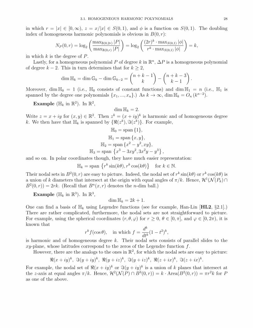
Example (Hk in R2). In R2,dimHk = 2.

Write z = x + iy for (x, y) ∈ R2. Then zk = (x + iy)k is harmonic and of homogeneous degreek. We then have that Hk is spanned by <(zk),=(zk). For example,

H0 = span 1,H1 = span x, y,

H2 = span x2 − y2, xy,H3 = span

x3 − 3xy2, 3x2y − y3

,

and so on. In polar coordinates though, they have much easier representation:

Hk = spanrk sin(kθ), rk cos(kθ)

for k ∈ N.

Their nodal sets in B2(0, r) are easy to picture. Indeed, the nodal set of rk sin(kθ) or rk cos(kθ) isa union of k diameters that intersect at the origin with equal angles of π/k. Hence, H1(N (Pk)∩B2(0, r)) = 2rk. (Recall that Bn(x, r) denotes the n-dim ball.)

Example (Hk in R3). In R3,dimHk = 2k + 1.

One can find a basis of Hk using Legendre functions (see for example, Han-Lin [HL2, §2.1].)There are rather complicated, furthermore, the nodal sets are not straightforward to picture.For example, using the spherical coordinates (r, θ, ϕ) for r ≥ 0, θ ∈ [0, π], and ϕ ∈ [0, 2π), it isknown that

rkf(cos θ), in which f =dk

dtk(1− t2)k,

is harmonic and of homogeneous degree k. Their nodal sets consists of parallel slides to thexy-plane, whose latitudes correspond to the zeros of the Legendre function f .

However, there are the analogs to the ones in R2, for which the nodal sets are easy to picture:

<(x+ iy)k, =(y + iy)k, <(y + iz)k, =(y + iz)k, <(z + ix)k, =(z + ix)k.

For example, the nodal set of <(x + iy)k or =(y + iy)k is a union of k planes that intersect atthe z-axis at equal angles π/k. Hence, H2(N (P ) ∩ B3(0, r)) = k · Area(B2(0, r)) = πr2k for Pas one of the above.


Example (Hk in Rn). In Rn,

dimHk = On

(kn−2

)as k →∞.

In this space of large dimension, most homogeneous harmonic polynomials have complicatednodal sets, which can not be computed explicitly. However, again the analogs to the ones in R2

have easy nodal portrait:

<(xj + ixl)k and =(xj + ixl)

k, j 6= l. (3.1)

Indeed, the nodal set of <(xj + ixl)k or =(xj + ixl)

k is a union of k hyperplanes that intersect atthe xj = xl = 0 at equal angles π/k. Hence, Hn−1(N (P )∩Bn(0, r)) = k · Hn−1(Bn−1(0, r)) =αn−1r

n−1k for Pk in (3.1).Therefore, we verify that the nodal size in Bn(x, r) of the homogeneous harmonic polynomials

in (3.1) are controlled by their doubling index:

Hn−1(N (P ) ∩Bn(0, r)) = αn−1rn−1k = αn−1r

n−1NP (0, r).

For general homogeneous harmonic polynomials, it is impossible to verify the nodal sizedirectly, especially as we are interested in the limit as k →∞. We next use the powerful integralgeometric formula to establish a general theorem.

Theorem 3.2 (Integral geometric formula). Let Pj : Rn → R be the projection from Rn tothe one deleting the j-th variable, i.e.,

Pj(x1, ..., xn) = (x1, ..., xj−1, xj+1, ..., xn).

Suppose that E is a smooth (n− 1)-dim hypersurface in Rn. Write

aj =

ˆRn−1

H0(E ∩ P−1j (y)) dy.

Then (n∑j=1

a2j

) 12

≤ Hn−1(E) ≤n∑j=1

aj.

See Han-Lin [HL2, Theorem 1.2.10] for more background of the integral geometric formula.In particular, it has a clear geometric interpretation: To estimate the size of an (n − 1)-dimobject in Rn, we only need to examine the intercepts of this set with all straight lines parallelto axis.

Theorem 3.3 (Upper bound of the nodal size of homogeneous harmonic polynomials). Forany P ∈ Hk in B(0, r), we have that

Hn−1(N (P ) ∩B(0, r)) ≤ C · rn−1k = C · rn−1NP (0, r),

in which C = C(n) = nαn−1.

That is, Conjecture 3.1 holds for homogeneous harmonic polynomials in B(0, r).

Proof. Fix y = (y1, ..., yj−1, yj+1, ..., yn) ∈ Rn−1. If

(y1, ..., yj−1, t, yj+1, ..., y) ∈ N (P ) ∩ P−1j (y).

thenPy(t) := P (y1, ..., yj−1, t, yj+1, ..., y) = 0.

3.2. LOWER BOUND OF THE NODAL SIZE: TAKE I 30

Observe that Py(t) is a single-variable polynomial of degree at most k since P ∈ Hk. Therefore,by the fundamental theorem of algebra,

H0(N (P ) ∩ P−1j (y)) = #t : Py(t) = 0 ≤ k.

Hence, in B(0, r),

aj =

ˆRn−1

H0(N (P ) ∩ P−1j (y)) dy ≤

ˆBn−1(0,r)

k dy = αn−1rn−1k.

Applying the integral geometric formula in Theorem 3.2, this theorem follows.

Remark.

• The first half of the inequality in Theorem 3.3 in fact holds for all polynomials, i.e. thenodal size of all polynomials of degree k in B(0, r) is bounded by Crn−1k. See Problem3-2. Therefore, the additional message of the theorem is that for homogeneous harmonicpolynomials, the degree equals the doubling index in B(0, r).• The constant C = nαn−1 (for example, C2 = 4) in Theorem 3.3 is unlikely sharp. In

fact, Guth [Gu, Example 2 on Page 1794] conjectured that the sharp constant is αn,which is achieved by <(xj + ixk)

k and =(xj + ixk)k for j 6= k (for example, rk sin(kθ)

and rk cos(kθ) in R2).• To understand the potential “overuse” of integral geometric formula, we apply Theorem

3.3 to rk sin(kθ) and rk cos(kθ). One sees that the number of zeros of Py(t) rarelysaturates the degree k. However, the difficulty to prove Guth’s conjecture is to designa more efficient integral geometric formula, potentially involving different “test curves”other than the lines parallel to axes in Theorem 3.2.

Problems .3-1. Prove that

Hn−1(N (P ) ∩B(0, r)) ≤ nαn−1 · rn−1k

for all polynomials P of degree k. (Hint: Repeat the proof of Theorem 3.3.)3-2. Find examples of polynomials P such that

Hn−1(N (P ) ∩B(0, 1)) = αn−1 · rn−1k.

3-3. Find examples of polynomials P such that the nodal set N (P ) = ∅.

3.2. Lower bound of the nodal size: Take I

Theorem 3.3 does not provide any lower bound on the nodal size of the polynomials, eventhough the integral geometric formula in Theorem 3.2 contains a lower bound. This is becausethe fundamental theorem of algebra does not give useful lower bound of number of zeros ofpolynomials in the real domain. In fact, a polynomial may have no zeros in the real domain.(See Problem 3-3.) This reflects the difficulty of the following conjecture.

Conjecture 3.4 (Lower bound of the nodal size of harmonic functions). There is a positiveconstant c = c(n) such that

Hn−1(N (u) ∩B(x0, r)) ≥ c · rn−1

for all harmonic functions u in B(x0, r) with u(x0) = 0.

See Nadirashvili [N] for the original text.

3.2. LOWER BOUND OF THE NODAL SIZE: TAKE I 31

Remark. The lower bound may be invalid without the condition that the function vanishesat some point. For example, u = 1 is harmonic but has no zeros. In fact, given any harmonicfunction u in a ball B, let M = supB |u|. Then v(x) := u(x) + M + 1 is harmonic but has nozeros in B.

In this section, we prove Conjecture 3.4 in R2. It is a direct consequence of the maximalprinciple of the harmonic functions.

Theorem 3.5 (Lower bound of the nodal size of harmonic functions in R2). We have that

H1(N (u) ∩B(x0, r)) ≥ r

for all harmonic functions u in B(x0, r) with u(x0) = 0.

Proof. Without loss of generality, we assume that x0 = (0, 0). (If not, then consider theharmonic function v(x) = u(x− x0).)

Since u(x0) = 0, the vanishing order Vu(x0) := d ≥ 0. Since u is analytic by Theorem 2.13and u(x0) = 0, we have that

u(x) =∞∑j=1

Pj(x) = Pd+1(x) +R(x),

in which Pd+1 is a homogeneous polynomial of degree d + 1 and R(x) = O(|x|d+2

)as x → 0.

That is, the Taylor expansion of u at x0 begins from the (d + 1)-th order term. Because u isharmonic, Pd+1 is also harmonic.

From Section 3.1, the nodal set of Pd+1 in B(x0, r) is a union of d diameters which intersectat x0 with equal angles of π/(d+ 1). Therefore, the nodal set of u near x0 is a union of d curves(which also intersect at x0 with equal angles of π/(d+ 1).)

Choose l as one of the nodal curves that passes through x0.Case 1. If l forms a closed loop, then denote the interior of this loop by Ω. Hence, u = 0 on

∂Ω = l. By the maximal principles of the harmonic functions in Theorem 2.3, u = 0 in Ω. (Infact, since u is analytic, u = 0 in B(x0, r).) The lower bound readily follows. Indeed,

H1(N (u) ∩B(x0, r)) ≥ H1(Ω) ≥ ∞,since Ω is 2-dim.

Case 2. If l extends to the boundary ∂B(x0, r) = S(x0, r), then l connects x0 with S(x0, r).Hence,

H1(N (u) ∩B(x0, r)) ≥ H1(l) ≥ dist(x0, S(x0, r)) = r.

Remark.

• The above argument of the lower bound breaks down in Rn for n ≥ 3. For example,let x0 = (0, 0, 0) and u be harmonic in B(x0, r) ⊂ R3 with u(x0) = 0. By the maximalprinciple, any surface s that contains x0 can not be closed in B(x0, r) unless u = 0in B(x0, r) and we are done. In the case when s extends to the boundary S(x0, r),there is no useful lower bound of the surface area H2(s). Indeed, one can have a verynarrow surface with arbitrarily small girth and therefore arbitrarily small surface areathat contains x0 and extends to S(x0, r). (Imagine a very thin finger that touches thecenter from outside of the ball.) Hence, the lower bound in Conjecture 3.4 does notfollow directly from the maximal principle.• Even for harmonic polynomials in Rn, the lower bound in Conjecture 3.4 is challenging.

See Appendix A for more discussion.

3.3. HARMONIC POLYNOMIALS 32

• Conjecture 3.4 in Rn for all n ≥ 3 has recently been solved by Logunov [Lo2]. In fact,Logunov established the lower bound for solutions to general elliptic PDEs (includingthe harmonic functions). The argument in [Lo2] is related to the upper bound discussedin this note but is beyond the scope of our coverage.

Recall in Chapter 2 that u(x, t) = φ(x)e√λt is harmonic in Rn+1 if φ is an eigenfunction in Rn

with eigenvalue λ > 0. Their nodal sets are also related in a simple fashion. We now present animmediate consequence of Conjecture 3.4 on the lower bound of the nodal size of eigenfunctionsin Yau’s conjecture 1.1.

Corollary 3.6 (Lower bound of the nodal size of eigenfunctions). There is a positiveconstant c = c(n) such that

Hn−1(N (φ) ∩B(x0, r)) ≥ c · rn−1λ12

for all eigenfunctions φ in B(x0, r), −∆φ = λφ with λ sufficiently large.

Proof. We know from Corollary 2.11 that the nodal set of φ is “λ−1/2 dense” in B(x0, r/2).

Therefore, one can find a maximal collection of disjoint balls B(xj, t) ⊂ B(x0, r/2) with t = r/√λ

such that φ(xj) = 0, j = 1, ..., N . Here, from the maximality of the collection,

N ≥ c · rn

tn,

in which c = c(n) depends only on the dimension.

Let u(x, t) = φ(x)e√λt. Fix B(xj, t). Then u(x, t) is harmonic in B(xj, t) × [−t, t] and

u(xj, 0) = φ(xj) = 0. By Conjecture 3.4,

Hn(N (u) ∩B(xj, t)× [−t, t]) ≥ ctn.

So

Hn−1(N (φ) ∩B(xj, t)) =1

2t· Hn(N (u) ∩B(xj, t)× [−t, t]) ≥ ctn−1.

Hence,

Hn−1(N (φ) ∩B(x0, r)) ≥ Hn−1(N (φ) ∩B(x0, r/2))

≥N∑j=1

Hn−1(N (φ) ∩B(xj, t))

≥ c · rn

tn· tn−1

≥ c · rnt−1

= c · rn−1λ12 .

3.3. Harmonic polynomials

In Section 3.1, we study the homogeneous harmonic polynomials. We showed that in B(0, r),their nodal size is always bounded above by the degree, which equals the doubling index inB(0, r). The natural questions are what happens in general balls if the center is not necessarilythe origin and how about the harmonic polynomials (not necessarily homogeneous).


Recall our notation that z = x + iy. Let Pk = =(zk) = rk sin(kθ) in the polar coordinates,which is a homogeneous harmonic polynomial. In the ball B(p, 1) centered at p = (k, 0), wehave that

N (Pk) ∩B(p, 1) = (t, 0) : k − 1 < t < k + 1,which has size 2. That is, there is only one nodal diameter of Pk in B(p, 1). So the degree isnot an appropriate quantity to estimate the nodal size. However, the doubling index of Pk onB(p, 1) is

NPk(p, 1) = log2

(maxB(p,2) |Pk|maxB(p,1) |Pk|

)= log2

((k + 2)k

(k + 1)k

)≤ log2

((1 +

1

k + 1

)k+1)

= log2 e.

Hence, the doubling index remains the appropriate quantity to control the nodal size:

H1(N (Pk) ∩B(p, 1)) . NPk(p, 1).

The zero (0, 0) of Pk has vanishing order k − 1 but is far away from B(p, 1). Consequently, thiszero has no influence on the doubling index (or the nodal size) of Pk in B(p, 1). This exampleindicates that the doubling index of a polynomial P in B(p, r) only concerns the total vanishingorders of zeros near B(p, r), but not the zeros far away from B(p, r). In the extreme case when|p| k, B(p, r) is far away from the zero (0, 0). It may contain no nodal set of Pk and thedoubling index at these balls is also bounded by a uniform constant.

In this section, we briefly (and non-rigorously) discuss the harmonic polynomials (not neces-sarily homogeneous) in R2 and in R3 and motivate the relations among the degree, the doublingindex, and the nodal size.

3.3.1. Harmonic polynomials in R2. Consider the (non-homogeneous) harmonic poly-nomial in R2

Pk(z) = <((z − z1)k1 · · · (z − zm)km

),

in which z1, ..., zm ∈ B(0, 1/2) and k1 + · · ·+ km = k. See the following pictures.

< (z12) <((z − 1

4− 1

4i)12)


<((z − 1

4− 1

4i)4 (

z + 14

+ 14i)8)

and <((z − 1

4− 1

4i)2 (

z + 14

+ 14i)4 (

z + 14− 1

4i)6)

The zero zj in B(0, 1/2) with vanishing order kj − 1 accounts for 2kj nodal radials. In total,the nodal size

H1(N (Pk) ∩B(0, 1)) ≈ k.

To compute the doubling index, observe that

|(w − z1)k1 · · · (w − zm)km| ≈ |w|k for |w| 1

2.

Therefore,

NPk(0, 1) = log2

(maxB(0,2) |Pk|maxB(0,1) |Pk|

)≈ k,

which controls the nodal size.To test the effect of a zero far away from B(0, 1) on the doubling index and nodal size, we

add a factor (z − z0)k0 into the polynomial:

<((z − z1)k1 · · · (z − zm)km(z − z0)k0

), where |z0| 1.

Then the degree of this polynomial is k+ k0. However, as |z0| 1, (z− z0)k0 is almost constantnear B(0, 1). The doubling index and the nodal pattern are both unchanged in B(0, 1), i.e., itis still controlled by k1 + · · ·+ km. Summarizing our intuition:

The nodal size of harmonic polynomials P in B(p, r) is bounded above by the doubling indexNP (p, r), which is related to the total vanishing orders of zeros near B(p, r).

Moreover, such intuition leads to our partial answers to the two questions posed in thebeginning of this chapter, in the case of harmonic polynomials in R2:

(1). Monotonicity: NP (p, r1) . NP (p, r2) for r1 ≤ r2, since B(p, r2) may contain more zeros ofthe polynomial than B(p, r1) which results larger doubling index.

(2). Additivity: NP (p,R) &∑

j NP (pj, rj) for disjoint B(xj, rj) ⊂ B(x,R), since NP (p, r) ac-

counts for the total vanishing orders of zeros in B(p, r).

3.3.2. Harmonic polynomials in R3. The harmonic polynomials in R3 are much morediverse than the ones discussed in R2. We only mention

Pk(x, y, z) = <((x+ iy)k

)

3.4. MONOTONICITY OF THE FREQUENCY FUNCTION 35

and demonstrate the intricacy of the additivity of the doubling index. We know that NPk(0, r) =k. In fact, for any point p on the z-axis: p = (0, 0, z)

NPk(p, r) = log2

(maxB(p,2r) |Pk|maxB(p,r) |Pk|

)= k.

Take disjoint balls B(pj, rj) in B(0, R) such that pj are on the z-axis. Then the additivity ofdoubling index for these small balls

Nu(0, R) ≥∑j

Nu(pj, rj)

can never be true.This example is very special, but indicates that the additivity of the doubling index is

highly dependent on the relative positions of the small balls B(pj, rj) and large ball B(0, R). Inparticular, the additivity fails if the small balls B(pj, rj) are all on the same straight line.

However, the doubling index of Pk at B(p, r) drops if p is away from z-axis. That is, ifp = (x, y, z) such that |x+ iy| = L, then

NPk(p, r) = log2

(maxB(p,2r) |u|maxB(p,r) |u|

)= log2

(|L+ 2r|k

|L+ r|k

)≤ k log2

(1 +

r

L

),

in whichlog2

(1 +

r

L

) 1 if L r.

Hence, if the balls B(pj, rj) are scattered away from z-axis, the additivity is possible. In Sections3.6 and 3.7, we study the (weak) additivity when the small balls are placed according to certaingeometric rules.

3.4. Monotonicity of the frequency function

Definition (Frequency function). Let u ∈ C0(Ω). For B(x, r) ⊂ Ω, define

Hu(x, r) =

ˆS(x,r)

|u(y)|2 dSy.

Then the frequency of u in B(x, r) is defined as

Fu(x, r) =rH ′u(x, r)

2Hu(x, r).

If there is only one function in question, then we omit the subscription u and write H(x, r) andF (x, r); if the center x is also fixed in the discussion, then we simply write H(r) and F (r).

Remark (Frequency function vs. doubling index). Recall that the doubling index of u onB(x, r) is defined by

Nu(x, r) = log2


).

It is closely related to the frequency function. In fact, we show in Theorem 3.12 that the doublingindex and the frequency functions of a harmonic function are indeed comparable. However,concerning the important properties:


(1). Monotonicity: For a fixed center x,

is Nu(x, r) or Fu(x, r) monotone in r?

It is more friendly to work with the frequency function Fu(x, r), since one can differentiatewith respect to r. In this section, we establish the crucial monotonicity formula for thefrequency function (Theorems 3.7 and 3.8). Since the doubling index is comparable withthe frequency function, the results in this section also yield monotonicity of the doublingindex in Section 3.5.

(2). Additivity: Let B(xj, rj) ⊂ B(x,R) be disjoint.

Is Nu(x,R) ≥∑j

Nu(xj, rj) or Fu(x,R) ≥∑j

Fu(xj, rj)?

It is more friendly to work with the doubling index Nu(x, r), since there are direct relationsamong the supremum of the functions on different balls, for example, maxB(xj ,rj) |u| ≤maxB(x,R) |u| since B(xj, rj) ⊂ B(x,R). From the examples of harmonic polynomials inSection 3.3, we already see that the additivity can not be expected in general. Nevertheless,in Sections 3.6 and 3.7, we establish certain weaker formulations of additivity.

Before proving the monotonicity formulas of the frequency function, we derive some equiva-lent forms of it. Since

Hu(x, r) =

ˆS(x,r)

|u(y)|2 dSy = rn−1

ˆB(0,1)

|u(x+ rz)|2 dSz,

we compute that

H ′u(x, r) = (n− 1)rn−2

ˆS(0,1)

|u(x+ rz)|2 dSz + 2rn−1

ˆS(0,1)

u(x+ rz)∂νu(x+ rz) dSz

=n− 1

r

ˆS(x,r)

|u(y)|2 dSy + 2

ˆS(x,r)

u(y)∂νu(y) dSy.

Hence,

Fu(x, r) =rH ′u(x, r)

2Hu(x, r)=n− 1

2+r´S(x,r)

u(y)∂νu(y) dSy´S(x,r)

|u(y)|2 dSy=n− 1

2+rDu(x, r)

Hu(x, r), (3.2)

in which

Du(x, r) =

ˆS(x,r)

u(y)∂νu(y) dSy.

Remark. The frequency function was initially introduced by Almgren [A]. See Han-Lin[HL2] for a complete treatment of frequency function and its application to the nodal setestimates of harmonic functions and eigenfunctions. The readers should be warned that thefrequency function in [A, HL2, Li] is slightly different from (3.2) in this note (which followsLogunov [Lo1, Lo2]). Indeed, for harmonic functions, the frequency function in [A, HL2, Li]is defined as

rDu(x, r)

Hu(x, r),

which differs with (3.2) by a constant (n− 1)/2. Such difference however has little effect on theresults discussed in this note.

We now prove the crucial monotonicity property for the frequency function.


Theorem 3.7 (Monotonicity of the frequency function). Let u be harmonic in B(x0, R).Then F (r) is increasing for r ∈ (0, R).

We use the simplified notations ∂j = ∂xj and ∂jk = ∂xj∂xk in the proof.

Proof. Without loss of generality, we assume that x0 = 0. (In the general case, let w(x) :=u(x+ x0). Then w is harmonic in B(0, R).) Since (3.2) reads

F (r) =rH ′(r)

2H(r)=n− 1

2+rD(r)

H(r),

it suffices to show that

F ′(r) =

(rD(r)

H(r)

)′=D(r)

H(r)+rD′(r)

H(r)− rD(r)H ′(r)

H(r)2=rD(r)

H(r)

(1

r+D′(r)

D(r)− H ′(r)

H(r)

)≥ 0.

To this end, we first estimate H ′(r): Since

H(r) =

ˆS(0,r)

|u(x)|2 dSx = rn−1

ˆB(0,1)

|u(ry)|2 dSy,

we compute that

H ′(r) = (n− 1)rn−2

ˆS(0,1)

|u(ry)|2 dSy + 2rn−1

ˆS(0,1)

u(ry)∂νu(ry) dSy

=n− 1

r

ˆS(0,r)

|u(x)|2 dSx + 2

ˆS(0,r)

u(x)∂νu(x) dSx

Hence,

H ′(r)

H(r)=n− 1

r+

2´S(0,r)

u(x)∂νu(x) dSx´S(0,r)

|u(x)|2 dSx.

Next, we estimate D′(r): Since u is harmonic,

D(r) =

ˆS(x,r)

u(x)∂νu(x) dSx =

ˆB(0,r)

|∇u(x)|2 dx,

by Green’s formula in Theorem 1.3. Hence,

D′(r) =

(ˆB(0,r)

|∇u(x)|2 dx)′

=

ˆS(0,r)

|∇u(x)|2 dSx

=1

r

ˆS(0,r)

|∇u(x)|2x · xrdSx

=1

r

n∑j=1

ˆS(0,r)

|∇u(x)|2xjxjrdSx

=1

r

n∑j=1

ˆS(0,r)

|∇u(x)|2xjνj(x) dSx,

in which for fixed j = 1, ..., n, we have thatˆS(0,r)

|∇u(x)|2xjνj(x) dSx


=

ˆB(0,r)

∂j(|∇u(x)|2xj

)dx (by fundamental theorem of calculus (1.3))

=

ˆB(0,r)

|∇u(x)|2 dx+ 2n∑k=1

ˆB(0,r)

xj∂ku(x)∂jku(x) dx

=

ˆB(0,r)

|∇u(x)|2 dx− 2n∑k=1

ˆB(0,r)

∂k(xj∂ku(x))∂ju(x) dx

+2n∑k=1

ˆS(0,r)

xj∂ku(x)∂ju(x)νk(x) dx (by integration by parts (1.4))

=

ˆB(0,r)

|∇u(x)|2 dx− 2

ˆB(0,r)

(∂ju(x))2 dx− 2n∑k=1

ˆB(0,r)

xj∂kku(x)∂ju(x) dx

+2rn∑k=1

ˆS(0,r)

νj∂ku(x)∂ju(x)νk(x) dx(

since νj =xjr

)=

ˆB(0,r)

|∇u(x)|2 dx− 2

ˆB(0,r)

(∂ju(x))2 dx+ 2r

ˆS(0,r)

νj∂ju(x)∂νu(x) dx (since ∆u = 0).

Summing over k, we get

D′(r)

=1

r

n∑j=1

ˆS(0,r)

|∇u(x)|2xjνj(x) dSx

=1

r

n∑j=1

(ˆB(0,r)

|∇u(x)|2 dx− 2

ˆB(0,r)

(∂ju(x))2 dx+ 2r

ˆS(0,r)

νj∂ju(x)∂νu(x) dx

)

=n

r

ˆB(0,r)

|∇u(x)|2 dx− 2

ˆB(0,r)

n∑j=1

(∂ju(x))2 dx+ 2

ˆS(0,r)

∂νu(x)n∑j=1

νj∂ju(x) dx

=n− 2

r

ˆB(0,r)

|∇u(x)|2 dx+ 2

ˆS(0,r)

|∂νu(x)|2 dx

=n− 2

rD(r) + 2

ˆS(0,r)

|∂νu(x)|2 dx.

Recall the Green formula in Theorem 1.3 that

D(r) =

ˆB(0,r)

|∇u(x)|2 dx =

ˆS(0,r)

u(x)∂νu(x) dx.

Hence,

D′(r)

D(r)=n− 2

r+

2´S(0,r)

|∂νu(x)|2 dx´S(0,r)

u(x)∂νu(x) dx.

Putting them together:

F ′(r) =rD(r)

H(r)

(1

r+D′(r)

D(r)− H ′(r)

H(r)

)


= 2N(r)

( ´S(0,r)

|∂νu(x)|2 dSx´S(0,r)

u(x)∂νu(x) dSx−

´S(0,r)

u(x)∂νu(x) dSx´S(0,r)

|u(x)|2 dSx

)≥ 0,

since (ˆS(0,r)

u(x)∂νu(x) dx

)2

≤ˆS(0,r)

|∂νu(x)|2 dx ·ˆS(0,r)

|u(x)|2 dSx

by the Cauchy-Schwarz inequality.

An immediate consequence is the following monotonicity formula.

Theorem 3.8 (Monotonicity formula of the frequency function). Let u be harmonic inB(x,R). Then for any 0 < r1 < r2 < R, we have that

H(r2) = H(r1) exp

(ˆ r2

r1

2F (r)

rdr

).

By Theorem 3.7, (r2

r1

)2F (r1)

≤ H(r2)

H(r1)≤(r2

r1

)2F (r2)

,

that is, (r2

r1

)2F (r1)

≤

´S(x,r2)

|u|2´S(x,r1)

|u|2≤(r2

r1

)2F (r2)

.

Furthermore, (r2

r1

)2F (r1)+1

≤

´B(x,r2)

|u|2´B(x,r1)

|u|2≤(r2

r1

)2F (r2)+1

.

Proof. Since F (r) = rH ′(r)/(2H(r)), H ′(r)/H(r) = rF (r)/2. Integrating both sides, wehave that

logH(r2)− logH(r1) =

ˆ r2

r1

2F (r)

rdr.

The equation in the theorem therefore follows. By Theorem 3.7, F (r1) ≤ F (r) ≤ F (r2) for allr ∈ [r1, r2]. Hence,

2F (r1) log

(r2

r1

)≤ˆ r2

r1

2F (r)

rdr ≤ 2F (r2) log

(r2

r1

).

The inequality about H(r) in the theorem follows. To prove the last inequalities, notice thatˆB(x,r2)

|u|2 =

ˆ r2

0

ˆS(x,r)

|u|2 dSdr

=r2

r1

ˆ r1

0

ˆS(x,tr2/r1)

|u|2 dSdt

≤ r2

r1

ˆ r1

0

(r2

r1

)2F (x,r2) ˆS(x,t)

|u|2 dSdt

≤(r2

r1

)2F (x,r2)+1 ˆ r1

0

ˆS(x,t)

|u|2 dSdt


=

(r2

r1

)2F (x,r2)+1 ˆB(x,r1)

|u|2,

which implies the upper bound in the last inequalities. The lower bound can be proved similarly.

After proving the monotonicity of the frequency function Fu(x, r) for fixed center, a naturalquestion involves the frequency function at different centers. To this end, we prove the followingtheorem.

Theorem 3.9. Let K ≥ 3 and u be harmonic in B (x,Kr). Then for any y ∈ B(x, r) and2 ≤ t ≤ K − 1, we have that

Fu(y, tr) ≤t logK

K − 1Fu (x,Kr) +

t logK

2(K − 1)− 1

2.

If 0 < t ≤ 2, then we apply the monotonicity of the frequency function and get

Fu(y, tr) ≤ Fu(y, 2r) ≤2 logK

K − 1Fu (x,Kr) +

logK

K − 1− 1

2≤ c1Fu (x,Kr) + c2,

in which c1 = c1(K) and c2 = c2(K) are positive constants that depend only on K.

Proof. Since y ∈ B(x, r) and 2 ≤ t ≤ K − 1,

B (x, r) ⊂ B(y, tr) ⊂ B (y, (K − 1)r) ⊂ B (x,Kr) .

Using Theorem 3.8, we have thatˆB(y,(K−1)r)

|u|2 ≤ˆB(x,Kr)

|u|2

≤ K2Fu(x,Kr)+1

ˆB(x,r)

|u|2

≤ K2Fu(x,Kr)+1

ˆB(y,tr)

|u|2.

Therefore, ´B(y,(K−1)r)

|u|2´B(y,tr)

|u|2≤ K2Fu(x,Kr)+1.

Using Theorem 3.8 again, ´B(y,(K−1)r)

|u|2´B(y,tr)

|u|2≥(K − 1

t

)2Fu(y,tr)+1

.

Hence, (K − 1

t

)2Fu(y,2r)+1

≤ K2Fu(x,Kr)+1,

which implies that

Fu(x, tr) ≤t logK

K − 1Fu (x,Kr) +

t logK

2(K − 1)− 1

2.

3.5. MONOTONICITY OF THE DOUBLING INDEX 41

3.5. Monotonicity of the doubling index

For general harmonic functions, we first note that if u is harmonic in a neighborhood of x,then Nu(x, r)→ d+ 1 as r → 0 if Vu(x) = d, i.e., u vanishes at x of order d. Indeed, let u havevanishing order d at x. Then ∂αu(x) = 0 for all |α| ≤ d and there is α with |α| = d + 1 suchthat ∂αu(x) 6= 0. By the Taylor expansion,

u(y) =∑|α|=d+1

∂αu(x)(y − x)α

α!+R(y − x) := P (y − x) +R(y − x),

in which the summation defines a homogeneous polynomial P of degree d+ 1 and the remainderR(y − x) = O

(|y − x|d+2

). One then deduces that Nu(x, r)→ NP (x, r) = d+ 1 as r → 0.

In this section, we prove the monotonicity properties for the doubling index, with the help offrequency function. We first see that the frequency function equals the degree (and therefore thedoubling index) module a constant (n− 1)/2 for homogeneous harmonic polynomials in B(0, r).

Theorem 3.10. For each P ∈ Hk in Rn, FP (0, r) = k + (n − 1)/2 = NP (0, r) + (n − 1)/2for all r > 0.

Proof. Write in the spherical coordinates:

P (r, θ) = rkφ(θ), r ∈ [0,∞), θ ∈ S(0, 1).

Notice that ∂ν = ∂r on S(0, r). Then

∂νP (r, θ) = ∂rP (r, θ) = krk−1φ(θ).

Then ˆS(0,r)

P∂νP dS =

ˆS(0,r)

rkφ(θ) · krk−1φ(θ) dS =k

r

ˆS(0,r)

|P |2 dS.

Hence,

FP (0, r) =n− 1

2+r´S(0,r)

P∂νP dS´S(0,r)

|P |2 dS= k +

n− 1

2.

We next prove a similar (but less precise) comparison between the frequency function andthe doubling index for all harmonic functions. First we need a lemma.

Lemma 3.11. Let δ > 0. Then

supB(x,r)

w ≤ maxB(x,r)

w ≤(

1 + δ

δ

)n S(x,(1+δ)r)

w dS

for all subharmonic and non-negative functions w in B(x, (1 + δ)r).

Proof. By Problem 2-2,

w(x) ≤ B(x,r)

w(y) dy.

In fact, we have that S(x,r)

w(y) dSy =1

nαnrn−1

ˆS(x,r)

w(y) dSy is increasing in r.

Hence, ˆB(x,r)

w(y) dy =

ˆ r

0

(ˆS(x,t)

w(y) dSy

)dt


=

ˆ r

0

(nαnt

n−1

S(x,t)

w(y) dSy

)dt

≤ S(x,r)

w(y) dSy

ˆ r

0

nαntn−1 dt

≤ αnrn

S(x,r)

w(y) dSy

=r

n

ˆS(x,r)

w(y) dSy.

For any y ∈ B(x, r), B(y, δr) ⊂ B(x, (1 + δ)r). Since w is non-negative,

w(y) ≤ B(y,δr)

w(z) dz

≤ 1

αnδnrn

ˆB(y,δr)

w(z) dz

=1

αnδnrn

ˆB(x,(1+δ)r)

w(z) dz

≤ 1 + δ

nαnδnrn−1

ˆS(x,(1+δ)r)

w(z) dz

=

(1 + δ

δ

)n S(x,(1+δ)r)

w(z) dz.

Theorem 3.12 (Comparison between the doubling index and the frequency function ofharmonic functions). Let ε > 0 be small. Then

(1− log2(1 + ε))Fu(x, (1 + ε)r)− 1

2log2

(1 + ε

εn

)− n− 1

2≤ Nu(x, r)

≤ (1 + log2(1 + ε))Fu(x, 2(1 + ε)r) +1

2log2

(1 + ε

εn

)− n− 1

2

for all harmonic functions u in B(x, 2(1 + ε)r). In particular, observe that log2(1 + ε) < 10ε.Denote

C = C(ε, n) =1

2log2

(1 + ε

εn

)+n− 1

2.

Then(1− 10ε)Fu(x, (1 + ε)r)− C ≤ Nu(x, r) ≤ (1 + 10ε)Fu(x, 2(1 + ε)r) + C.

Proof of Theorem 3.12. By Problem 2-1, |u|2 is subharmonic. By the Lemma 3.11,

maxB(x,2r)

|u|2 ≤(

1 + ε

ε

)n S(x,2(1+ε)r)

|u|2 dS =1 + ε

εn· Hu(x, 2(1 + ε)r)

nαn2n−1rn−1.

On the other hand, since S(x, r) ⊂ B(x, r),

maxB(x,r)

|u|2 ≥ supS(x,r)

|u|2 ≥ S(x,r)

|u(y)|2 dy =Hu(x, r)

nαnrn−1.


Using the monotonicity formula in Theorem 3.8,

Hu(x, 2(1 + ε)r)

Hu(x, r)≤ (2(1 + ε))2Fu(x,2(1+ε)r).

Therefore,

Nu(x, r) =1

2log2

(maxB(x,2r) |u|2

maxB(x,r) |u|2

)≤ 1

2log2

(Hu(x, 2(1 + ε)r)

Hu(x, r)· (1 + ε)

2n−1εn

)≤ 1

2log2

(Hu(x, 2(1 + ε)r)

Hu(x, r)

)+

1

2log2

(1 + ε

εn

)− n− 1

2

≤ log2(2(1 + ε))Fu(x, 2(1 + ε)r) +1

2log2

(1 + ε

εn

)− n− 1

2

≤ (1 + log2(1 + ε))Fu(x, 2(1 + ε)r) +1

2log2

(1 + ε

εn

)− n− 1

2.

To obtain the opposite estimate of Nu and Fu, see Problem 3-4.

An immediate consequence is the monotonicity property of the doubling index:

Theorem 3.13 (Monotonicity of the doubling index). Let ε > 0. There is constant C =C(ε, n) such that if r2 ≥ 2r1 > 0, then

Nu(x, r2) ≥ (1− ε)Nu(x, r1)− Cfor all harmonic functions u in B(x, 2r2).

This theorem is obviously weaker than the monotonicity of the frequency function in Theorem3.7.

Proof. By Theorem 3.7, there is constant C1 = C1(ε1, n) > 0 such that

(1− 10ε1)Fu(x, (1 + ε1)r)− C1 ≤ Nu(x, r) ≤ (1 + 10ε1)Fu(x, 2(1 + ε1)r) + C1.

By the monotonicity of the frequency function in Theorem 3.7, since r2 ≥ 2r1,

Nu(x, r2) ≥ (1− 10ε1)Fu(x, (1 + ε1)r2)− C1

≥ (1− 10ε1)Fu(x, 2(1 + ε1)r1)− C1

≥ 1− 10ε1

1 + 10ε1

Nu(x, r1)− 2C1

1 + 10ε1

≥ (1− ε)Nu(x, r1)− C,by setting ε1 = ε/40 and C = 2C1/(1 + 10ε1).

Next we prove the monotonicity formula for the doubling index that is similar to Theorem3.8 for the frequency function.

Theorem 3.14 (Monotonicity formula of the doubling index). Let ε > 0 be small. Thenthere exists C = C(ε, n)→∞ depending only on ε→ 0 (and the dimension n) such that

t(1−ε)Nu(x,r)−C ≤maxB(x,tr) |u|maxB(x,r) |u|

≤ t(1+ε)Nu(x,tr)+C


for all harmonic functions u in Ω and B(x, tr) ⊂ Ω. In addition, there is N0 = N0(ε, n) suchthat if Nu(x, r) ≥ N0, then

t(1−ε)Nu(x,r) ≤maxB(x,tr) |u|maxB(x,r) |u|

≤ t(1+ε)Nu(x,tr).

Proof. We only prove the lower bound, the upper bound can be proved similarly. We canassume that t > 21/(1−ε). Otherwise 2 ≤ t ≤ 21/(1−ε) so

maxB(x,tr)

|u| ≥ maxB(x,2r)

|u| ≥ 2Nu(x,r) maxB(x,r)

|u| ≥ t(1−ε)Nu(x,r) maxB(x,r)

|u|,

which implies the lower bound.First,

maxB(x,tr)

|u|2 ≥ supS(x,tr)

|u|2 ≥ S(x,tr)

|u(y)|2 dSy =Hu(x, tr)

nαntn−1rn−1. (3.3)

Since t > 21/(1−ε), (1− ε)tr > 2(1 + ε)r. By the monotonicity formula for the frequency functionin Theorem 3.8,

Hu(x, tr) ≥(

t

2(1 + ε)

)2Fu(x,2(1+ε)r)

·Hu(x, 2(1 + ε)r)

≥(

t

2(1 + ε)

) 2Nu(x,r)1+10ε

− 2C1+10ε

·Hu(x, 2(1 + ε)r),

in which we use Theorem 3.12 that

(1 + 10ε)Fu(x, 2(1 + ε)r) + C ≥ Nu(x, r).

Second, using the definition of doubling index,

maxB(x,2r)

|u| = 2Nu(x,r) maxB(x,r)

|u|,

So by Lemma 3.11,

maxB(x,r)

|u|2 = 2−2Nu(x,r) maxB(x,2r)

|u|2

≤ 2−2Nu(x,r)

(1 + ε

ε

)n S(x,2(1+ε)r)

|u(y)|2 dSy

≤ 2−2Nu(x,r) · (1 + ε)Hu(x, 2(1 + ε)r)

nαn2n−1εnrn−1,

which implies that

Hu(x, 2(1 + ε)r) ≥ 22Nu(x,r)nαn2n−1εnrn−1

1 + εmaxB(x,r)

|u|2.

Connecting (3.3) with the subsequent estimates, we have that

maxB(x,tr)

|u|2

≥ 1

nαntn−1rn−1·Hu(x, tr)

≥ 1

nαntn−1rn−1·(

t

2(1 + ε)

) 2Nu(x,r)1+10ε

− 2C1+10ε

·Hu(x, 2(1 + ε)r)


≥ 22Nu(x,r)nαn2n−1εnrn−1

nαn(1 + ε)tn−1rn−1·(

t

2(1 + ε)

) 2Nu(x,r)1+10ε

− 2C1+10ε

· maxB(x,r)

|u|2

≥ 2n−1εn

1 + ε·(

t

1 + ε

) 2Nu(x,r)1+10ε

− 2C1+10ε

· t−(n−1) · maxB(x,r)

|u|2

= 2n−1εn(1 + ε)2C

1+10ε−1 ·

(1

1 + ε

) 2Nu(x,r)1+10ε

· t2Nu(x,r)1+10ε

− 2C1+10ε

−(n−1) · maxB(x,r)

|u|2.

Since t ≥ 2, one can choose C1 = C1(ε, n) > 0 large enough such that

2n−1εn(1 + ε)2C

1+10ε−1 ≥ 2−C1 ≥ t−C1 .

In addition, as ε→ 0+, there is ε1 = ε1(ε)→ 0+ such that

1

1 + ε≥ 2−ε1 ≥ t−ε1 .

Hence,

maxB(x,tr)

|u|2 ≤ t2(1−ε1)Nu(x,r)

1+10ε− 2C

1+10ε−(n−1)−C1 · max

B(x,r)|u|2,

which implies thatmaxB(x,tr) |u|maxB(x,r) |u|

≥ t(1−ε)Nu(x,r)−C

with appropriate (new) ε and C.

Similar to Theorem 3.9 that compares the frequency function at different centers, we have

Theorem 3.15. Let δ ∈ (0, 1). Then there exist positive constants K = K(δ) ≥ 1 andN0 = N0(δ, n) such that if Nu(x, r) ≥ N0, then for any y ∈ B(x, r), we have that

Nu (y, 2Kr) ≥ (1− δ)Nu(x, r)

for all harmonic functions u in B (x, (2K + 1)r).

Proof. Using Theorem 3.13, there is C = C(ε1, n) such that

Nu (x, (K + 1)r) ≥ (1− ε1)Nu(x, r)− C,because K + 1 ≥ 2. Since y ∈ B(x, r),

B (y,Kr) ⊂ B(x, (K + 1)r) and B (x, (2K − 1)r) ⊂ B (y, 2Kr) .

Using Theorem 3.14, we have that if Nu (x, (K + 1)r) ≥ N2 = N2(ε2, n), then

2(1+ε2)Nu(y,2Kr) ≥maxB(y,2Kr) |u|maxB(y,Kr) |u|

≥maxB(x,(2K−1)r) |u|maxB(x,(K+1)r) |u|

≥(

2K − 1

K + 1

)(1−ε2)Nu(x,(K+1)r)

.

See (4) below for the choice of the parameters so the condition Nu (x, (K + 1)r) ≥ N2 is met.Therefore,

Nu (y, 2Kr) ≥ 1− ε2

1 + ε2

· log2

(2K − 1

K + 1

)·Nu (x, (K + 1)r)

3.6. THE SIMPLEX LEMMA 46

≥ (1− ε2)(1− ε1)

1 + ε2

· log2

(2K − 1

K + 1

)·Nu(x, r)− C

Let δ > 0. We now choose the parameters to finish the proof.

(1). Choose ε2 = ε2(δ) > 0 small enough so

1− ε2

1 + ε2

≥ 1− δ

4.

(2). Choose ε1 = ε1(δ) > 0 small enough so

(1− ε2)(1− ε1)

1 + ε2

≥ 1− δ

3.

(3). Choose K = K(δ) > 0 large enough so

(1− ε2)(1− ε1)

1 + ε2

· log2

(2K − 1

K + 1

)≥ 1− δ

2.

(4). Choose N0 = N0(δ, n) > 0 large enough such that if Nu(x, r) ≥ N0, then

Nu (x, (K + 1)r) ≥ (1− ε1)Nu(x, r)− C ≥ (1− ε1)N0 − C ≥ N2,

and (1− δ

2

)Nu(x, r)− C ≥ (1− δ)Nu(x, r).

Problems .3-4. Prove the lower bound in Theorem 3.12.

3.6. The simplex lemma

We summarize the main themes of monotoninicity of the doubling index Nu(x, r) in Section3.5 for harmonic functions:

(i). “Nu(x, r) with fixed center x is increasing in r.” – It is put in quotations since this is onlymorally true. See Theorem 3.13 for details.

(ii). “Nu(x, r2) and Nu(x, r1) characterize the growth rate of |u| from B(x, r1) to B(x, r2) forr1 ≤ r2”: (

r2

r1

)Nu(x,r1)

≤maxB(x,r2) |u|maxB(x,r1) |u|

≤(r2

r1

)Nu(x,r2)

.

Again, it is put in quotations since the above inequalities are also only morally true. SeeTheorem 3.14 for details.

In this section, we investigate the additivity property of the doubling index of harmonicfunctions: Let B(xj, rj) ⊂ B(x,R) be disjoint. Is

Nu(x,R) ≥∑j

Nu(xj, rj)?

From the example (x + iy)k in R3 discussed in Section 3.3, we see that without any geometricconstraints, it can fail (for example, if the centers xj are on the same line). That is, the additivityproperty is highly dependent on the relative geometric positions of the balls.

In fact, it is extremely challenging to prove any kind of additivity result for harmonic func-tions. For example, the most fundamental additivity question asks: Given B(xj, rj) such that


Nu(xj, rj) = N , can one find B(x0, R) such that Nu(x0, R) > N , that is, can the doubling indexof B(xj, rj) “add up” at B(x0, R) by a bit?

The simplex lemma in this section provide an answer to this fundamental question. That is, ifxj are the vertices of a non-degenerate simplex (that is, the simplex does not lie in a hyperplane,in particular, xj are not on the same line,) then the doubling index at the barycenter x0 of thesimplex is strictly greater than the ones at the vertices.

Remark (Intuition of the proof of the simplex lemma). Both of the upper and lower boundsof the growth rate of |u| in terms of the doubling index are provided in Theme (ii) above. Thisis the starting point of the proof. That is, let B(x0, R1) grow to B(x0, R2) and B(xj, r1) growto B(xj, r2). Then we aim to build a sequence of inequalities so Nu(x0, R2) can be bounded byNu(xj, r1) from below:(

R2

R1

)Nu(x0,R2)

≥maxB(x0,R2) |u|maxB(x0,R1) |u|

≥maxB(xj ,r2) |u|maxB(xj ,r1) |u|

≥(r2

r1

)Nu(xj ,r1)

.

In order for the middle inequality to hold, we need

(I).max

B(x0,R2)|u| ≥ max

B(xj ,r2)|u|,

which amounts to covering balls B(xj, r2) at the vertices by the ball B(x0, R2) at thebarycenter. It is done by Covering Lemma I below.

(II).max

B(x0,R1)|u| ≤ max

B(xj ,r1)|u|,

which amounts to covering the ball B(x0, R1) at the barycenter by the balls B(xj, r1) atthe the vertices. It is done by Covering Lemma II below.

3.6.1. The simplex geometric lemmas.

Definition (Euclidean simplexes). The n-simplex S with vertices x1, ..., xn+1 ∈ Rn is definedas the convex hull of x1, ..., xn+1, i.e.,

S = t1x1 + · · ·+ tn+1xn+1 : t1 + · · ·+ tn+1 = 1, t1, ..., tn+1 ≥ 0.For example, a 0-simplex is a point, a 1-simplex is a line segment, a 2-simplex is a triangle, a3-simplex is a tetrahedron (i.e., pyramid), and so on. Let S be an n-simplex in Rn.

• Denote diam(S) the diameter of S, i.e., the maximal distance between a pair of pointsin S.• Denote width(S) the width of S, i.e, the minimal distance between a pair of parallel

hyperplanes such that S is contained between them.• Denote ω(S) = width(S)/diam(S) ∈ [0, 1] the relative width of S. We say that the

simplex is degenerate (or flat) if ω(S) = 0. Abusing the terminology somehow, we saythat a simplex is more degenerate (or flat) if ω is smaller.• Define the barycenter x0 of S as

x0 =x1 + · · ·+ xn+1

n+ 1.

Keep the above notation throughout this subsection. The following two lemmas show certaincovering relations between balls centered at the vertices and balls centered at the barycenter.Later on we apply these covering lemmas to study the relation among the doubling indexes ofthese balls.


The first covering lemma says that balls with smaller radius can be covered by balls withlarger radius, and it therefore straightforward. It is an immediate consequence of the triangleinequality.

Lemma 3.16 (Covering Lemma I). Let S be an n-simplex and r > 0. Suppose that t > 0.Then

n+1⋃j=1

B(xj, tr) ⊂ B(x0, (1 + δ)tr),

for

δ =diam(S)

tr.

We remark that δ → 0 as t→∞, that is, as the radius tend to infinity, balls centered at thebarycenter and at the vertices are almost the same.

Proof. Let j = 1, ..., n and y ∈ B(xj, tr). By the triangle inequality,

|y − x0| < |y − xj|+ |xj − x0| ≤ tr + diam(S) ≤ (1 + δ)tr,

if

δ ≥ diam(S)

tr.

The second covering lemma says that balls with larger radius can be covered by balls withsmaller radius, and is therefore more complicated than the first lemma. It uses the property ofthe relative width of a simplex.

Lemma 3.17 (Covering Lemma II). Let a > 0. Then there exist c1 = c1(a, n) > 0 andK = K(a, n) ≥ 2/a such that

B(x0, (1 + c1)r) ⊂n+1⋃j=1

B(xj, r), in which r = K · diam(S)

for all simplexes S with the relative width ω(S) > a. In addition, c1 → 0+ and K → ∞ asa→ 0.

Remark.

• In the extreme case when ω(S) = 0 (i.e., S lies on a hyperplane), the above coveringproperty is impossible.• It is obvious that the above covering property is impossible if K is too small, sayK < 1/100, so B(xj, r) are tiny balls centered at the vertices and can never cover a ballcentered at the barycenter. The choice of K ≥ 2/a is mainly for future application inSection 3.8.

Proof. See Problems 3-5 and 3-6.

Using the two covering lemmas and the monotonicity formula in Theorem 3.14, we derivethe following simplex lemma. It is a weak form of additivity mentioned above. In particular, itasserts that the doubling index at the barycenter of a simplex must be at least slightly largerthan the ones at the vertices, if the simplex is not degeneration. In the view of the examplein the beginning of this section, the non-degeneracy of the simplex is necessary, that is, thisphenomenon of weak additivity can not be true if the simplex degenerates to a line segment.


Lemma 3.18 (The simplex lemma). Let a > 0 and K = K(a, n) ≥ 2/a. Suppose thatω(S) > a and r = K ·diam(S). Then there are positive constants c = c(a, n), C = C(a, n) ≥ K,and N0 = N0(a, n) such that if for each j = 1, ..., n + 1, Nu(xj, rj) ≥ N ≥ N0 for some0 < rj ≤ r/2, then

Nu (x0, C · diam(S)) > (1 + c)N

for all harmonic functions u.

Remark. We can call the simplex lemma a weak version of additivity of the doubling index:The doubling index at the vertices “add up” (a little bit) to the one at the barycenter.

Proof. By the weak monotonicity of the doubling index in Theorem 3.13, we can assumethat Nu(xj, r) ≥ N since r ≥ 2rj. Let

M = max∪n+1j=1 B(xj ,r)

|u|.

Then M = maxB(xj ,r) |u| for some j = 1, ..., n + 1. By the covering lemma in Lemma 3.17, wehave that

B(x0, (1 + c1)r) ⊂n+1⋃j=1

B(xj, r),

which implies thatmax

B(x0,(1+c1)r)|u| ≤M.

Let t, ε > 0, whose values will be specified later. By Theorem 3.14, if N ≥ N0, then

maxB(xj ,tr)

|u| ≥ t(1−ε)Nu(xj ,r) maxB(x,r)

|u| ≥Mt(1−ε)N .

By the covering lemma in Lemma 3.16,n+1⋃j=1

B(xj, tr) ⊂ B(x0, (1 + δ)tr),

in which δ = diam(S)/(tr) = 1/(Kt)→ 0 as t→∞. Therefore,

maxB(xj ,tr)

|u| ≤ maxB(x0,(1+δ)tr)

|u| for all j = 1, ..., n+ 1.

By Theorem 3.14 again,((1 + δ)t

1 + c1

)(1+ε)Nu(x0,(1+δ)tr)

≥maxB(x0,(1+δ)tr) |u|maxB(x0,(1+c1)r) |u|

≥maxB(xj ,tr) |u|

maxB(x0,(1+c1)r) |u|

≥ Mt(1−ε)N

M

= t(1−ε)N . (3.4)

Recall that a,K, c1 are fixed. Now we choose the four parameters t, δ, ε, C in order.

(1). Choose t > 2 so that δ = 1/(Kt) < c1/2. Then

1 + c1/2

1 + c1

= t−c2 ,

3.7. THE HYPERPLANE LEMMA 50

in which

c2 = logt

(1 + c1

1 + c1/2

)∈ (0, 1).

Hence,(1 + δ)t

1 + c1

≤ t(1 + c1/2)

1 + c1

= t1−c2 .

Then (3.4) reduces to

Nu(x0, (1 + δ)tr) ≥ 1− ε(1 + ε)(1− c2)

N.

(2). Choose ε ∈ (0, c2). Set c = (c2 − ε)/2. Hence,

1− ε(1 + ε)(1− c2)

≥ 1− ε1− c2

≥ 1 + c,

which implies that

Nu(x0, (1 + δ)tr) ≥ 1− ε(1 + ε)(1− c2)

N ≥ (1 + c)N.

(3). The lemma is done by choosing C = (1 + δ)tK.

Problems .3-5. Let S be an equilateral triangle in R2 with side-length l. Let x1, x2, x3 be the three

vertices and x0 be the barycenter. Find the relative width ω of S. Then prove that for all K > 1,there is positive constant c1 = c1(K) such that

B(x0, (1 + c1)r) ⊂3⋃j=1

B(xj, r), in which r = K · diam(S).

3-6. Prove Lemma 3.17. Try to prove it in R2 first.

3.7. The hyperplane lemma

Recall that the simplex lemma in Section 3.6 asserts that the doubling index at the vertices“add up” to the one at the barycenter for harmonic functions, if the simplex is non-degenerate.We also know, according to the example (x + iy)k, the non-degeneracy condition can not bedropped.

From now on, we work with cubes instead of balls. We use Q and q to denote cubes. Definethe doubling index of u at Q as

Nu(Q) = supx∈Q,r∈(0,diam(Q))

Nu(x, r) = supx∈Q,r∈(0,diam(Q))

log2


). (3.5)

If there is only one function in question, then we omit the subscription u.Notice that to define Nu(Q), we need u to be defined in a larger domain than Q, for example,

10nQ which is sufficiently large to contain B(x, 2r) for all x ∈ Q and r < diam(Q). Here, kQmeans the cube with the same center as Q and side-length as k times the side-length of Q.However, this issue will not concern us, as we will always assume that u is defined in a sufficientlylarge domain.


Remark. In the view of the doubling index of balls, it is probably more natural to definethe doubling index of cubes by

log2

(max2Q |u|maxQ |u|

).

However, such definition is not friendly for proving additivity (such as the simplex lemma inSection 3.6) or monotonicity.

Whereas the definition (3.5) of the doubling index of cubes has several advantages, includingthe immediate monotonicity property: If q ⊂ Q, then Nu(q) ≤ Nu(Q).

Remark (Cubes vs. balls). We provide a quick comparison between cubes and balls whenapplying to the additivity properties of the doubling index. Notice that cubes can be partitionedinto subcubes. In particular, let A ∈ N. Then a cube Q divides into An subcubes of equal size.While balls can not be partitioned into small balls, they are nicely suited for the covering lemmasin Section 3.6, which can be used to establish a certain form of additivity in the simplex lemma.

In summary,

• balls work well with covering properties as in Section 3.6 and the additivity appears inthe form of

the doubling index of small balls “add up” to the one of a big ball,

if the small balls are positioned at the vertices of a non-degenerate simplex.• cubes work well with partition properties as in this and next sections and the additivity

appears in the form of

the doubling index of subcubes “add up” to the one of the cube,

if the subcubes are positioned according to some geometric constraints.

In this section, we prove the hyperplane lemma. It asserts that if the doubling index on allthe subcubes q that are “on” the same hyperplane is greater than N , then the doubling indexon the big cube Q must “add up” to at least 2N . Again, similarly as for the simplex lemma inthe view of the example (x+ iy)k, the condition of the hyperplane can not be dropped.

Lemma 3.19 (The hyperplane lemma). Let Q = [−R/2, R/2]n ⊂ Rn. Divide Q into An

subcubes of equal size. Denote qj,0, j = 1, ..., An−1, the subcubes that intersect the hyperplanexn = 0. Then there are positive constants A0 = A0(n) and N0 = N0(n) such that if A ≥ A0 isodd and Nu(qj,0) ≥ N ≥ N0 for all qj,0, then

Nu(Q) > 2N


Remark.

• Here, we require A to be odd so there is no ambiguity in defining the subcubes thatintersect the hyperplane xn = 0, i.e., the ones whose centers are on xn = 0.• The hyperplane lemma remains valid if xn = 0 is replaced by any other hyperplane

that is parallel to one of the faces of the cube. This can be done by simply rotatingthe whole space and noticing that the harmonic functions are still harmonic after therotation.• The key idea to prove the hyperplane lemma is to apply the Cauchy uniqueness theorem,

that is, if a harmonic function u and its derivative ∂νu (i.e., the Cauchy data) are bothsmall on a piece of the hyperplane xn = 0, then u must be small in a neighborhood ofxn = 0. In the application to prove the hyperplane lemma, the doubling index of the


subcubes that intersect xn = 0 controls u and ∂νu on xn = 0. It in turn determinesthe size of u in a neighborhood of xn = 0, say Q/K for some large K. Then thedoubling index of Q is controlled, as it can be estimated by the growth rate of |u| fromQ/K to Q.• The hyperplane lemma follows from careful analysis of geometric objects such as cubes

as well as balls. In addition, it needs the quantitative Cauchy uniqueness theorem 2.16:There exist constant C > 0 and ε ∈ (0, 1) such that if a harmonic function u in qsatisfies

|u(x)| ≤ 1, if x ∈ q,|u(x)| ≤ ε, if x ∈ F,|∂νu(x)| ≤ ε

r, if x ∈ F,

for some ε ≥ 0, thensup12q

|u| ≤ Cεα.

Here, F is a face of q, r is the side-length of q, and 12q is the middle cube of q with half

side-length.

Proof of Lemma 3.19. Without loss of generality, we assume that R = 1. (In the generalcase, set v(x) = u(x/R) so v is harmonic in [−1/2, 1/2]n.) We divide the proof into four stepsaccording to the plan mentioned above. Denote

M = maxB(0,1/8)

|u|.

Step 1. Estimate |u| on a piece of the hyperplane xn = 0. Of course, |u(x)| ≤ M onthe piece B(0, 1/8) ∩ xn = 0. But this does not take into account of the doubling index nearthe hyperplane xn = 0. To exploit the doubling index, we consider max2qj,0 |u| and use it tocontrol |u(x)| for which x ∈ qj,0 so there is doubling action involved.

Notice that Nu(qj,0) ≥ N , there is xj ∈ qj,0 and rj < diam(qj) =√n/A such that Nu(xj, rj) ≥

N ≥ N0. Hence, elementary Euclidean geometry yields that

2qj,0 ⊂ B(xj,

4√n

A

).

Let x ∈ B(0, 1/16) ∩ xn = 0. Then there is qj,0 3 x such that qj,0 ⊂ B(0, 1/12) (if1/A < 1/12 − 1/16, i.e., A > 36). Thus, xj ∈ B(0, 1/12) and B(xj, 1/32) ⊂ B(0, 1/8) sincexj ∈ qj,0 ⊂ B(0, 1/12). Therefore, maxB(xj ,1/32) |u| ≤M .

We now require 4√n/A < 1/32, i.e., A ≥ A0(n) > 128

√n. Using the monotonicity formula

of doubling index in Theorem 3.14 with ε = 1/2,

maxB(xj ,1/32) |u|maxB

(xj ,

4√n

A

) |u| ≥(

A

128√n

)Nu

(xj,

4√n

A

)2

≥(

A

128√n

)Nu(xj,rj)

2

≥(

A

128√n

)N2

,

in which we also use the weak monotonicity of the doubling index in Theorem 3.13:

Nu

(xj,

4√n

A

)≥ Nu(rj, rj),

since rj < diam(qj,0) =√n/A. We then have that

max2qj,0|u| ≤ max

B(xj ,

4√n

A

) |u|


≤(

128√n

A

)N2

· maxB(xj , 1

32)|u|

≤(

128√n

A

)N2

·M.

Therefore, x ∈ B(0, 1/16) ∩ xn = 0,

|u(x)| ≤ max2qj,0|u| ≤

(128√n

A

)N2

·M.

Step 2. Estimate |∂νu| on B(0, 1/16) ∩ xn = 0. To this end, we use the estimates ofderivatives of harmonic functions in Theorem 2.8. That is,

|∂xju(x)| ≤ C1

rn+1

ˆB(x,r)

|u| = 4n

αnrn+1

ˆB(x,r)

|u|.

For x ∈ qj,0 ∩ xn = 0, we choose B(x, 1/A) ⊂ 2qj,0 in the above integral, where 1/A is theside-length of qj,0. That is,

|∂xju(x)| ≤ 4nA · maxB(x,1/A)

|u| ≤ 4nA ·max2qj,0|u|.

Using the estimate of max2qj,0 |u| in Step 1, we have that

|∂xju(x)| ≤ 4nA ·max2qj,0|u| ≤ 4nA

(128√n

A

)N2

·M

for all j = 1, ..., n. Therefore, for all x ∈ B(0, 1/16) ∩ xn = 0,

|∇u(x)| ≤n∑j=1

|∂xju(x)| ≤ 4n2A

(128√n

A

)N2

·M,

which of course also bounds |∂νu(x)|.Step 3. Application of the quantitative Cauchy uniqueness theorem. From Steps 1 and 2,

we know that on B(0, 1/16) ∩ xn = 0,

|u| ≤(

128√n

A

)N2

·M and |∂νu| ≤ 4n2A

(128√n

A

)N2

·M.

We see that

4n2A

(128√n

A

)N2

·M ≤M · 2−c1(n)N logA,

in which c1(n) is a positive constant depending only on n.Now we set up a cube q to apply the quantitative Cauchy uniqueness theorem. Let q be a

cube with side-length 1/(16√n) in the upper half space xn ≥ 0 such that q ⊂ B(0, 1/16) and

B(

0,1

32√n

)∩ xn = 0 ⊂ ∂q ∩ xn = 0 ⊂ B

(0,

1

16

)∩ xn = 0.

That is, q has a face F on the hyperplane xn = 0


Let v = u/M . Then |v| ≤ 1 in q. Moreover, on the face F ⊂ B(0, 1/16) ∩ xn = 0, noticethat the side-length of q is 1/(16

√n),

|v| ≤(

128√n

A

)N2

= 2−c(n)N logA := ε,

and

|∂νu| ≤ 4n2A

(128√n

A

)N2

=

n2A4√n·(

128√n

A

)N2

116√n

≤ ε1

16√n

,

in which c1(n) is a positive constant depending only on n.Using the quantitative Cauchy uniqueness theorem, |v| ≤ εα in q/2. So

max12q|u| ≤M · εα = M · 2−c1(n)αN logA.

Denote p the center of the cube q. Then since q/2 has side-length 1/(32√n),

B(p,

1

64√n

)⊂ 1

2q.

Somax

B(p, 1

64√n

) |u| ≤M · 2−c1(n)αN logA.

Step 4. Estimate Nu(p, 1/2) and Nu(Q). Recall that p is the center of q that satisfiesp ∈ B(0, 1/32). Then B(p, 1/2) ⊃ B(0, 1/8) so maxB(p,1/2) ≥M = maxB(0,1/8). Therefore,

maxB(p, 12) |u|

maxB(p, 1

64√n

) |u| ≥ 2c1(n)αN logA.

But according to the monotonicity formula of the doubling index in Theorem 3.14 with ε = 1/2,

maxB(p, 12) |u|

maxB(p, 1

64√n

) |u| ≤ (32√n)

32Nu(p,1/2) = 2c2(n)Nu(p,1/2),

in which c2(n) is a positive constant depending only on n. Putting the above two inequalitiestogether:

c2(n)Nu(p, 1/2) ≥ c1(n)αN logA,

which implies thatNu(p, 1/2) > 2N,

if A ≥ A0(n) is chosen large enough. The theorem is then completed by noticing that


Nu(x, r) ≥ N(p, 1/2).

By inductively applying the hyperplane lemma, we prove the following corollary.

Corollary 3.20. Let Q = [−R/2, R/2]n ⊂ Rn and ε > 0. Divide Q into An subcubes ofequal size. Denote qj,0, j = 1, ..., An−1, the subcubes that intersect the hyperplane xn = 0.Then there are positive constants A0 = A0(ε, n) and N0 = N0(n) such that if A ≥ A0 is odd andNu(Q) = N ≥ N0, then

#j : Nu(qj,0) ≥ N/2 < εAn−1



That is, among all the subcubes that intersect xn = 0, almost all subcubes (i.e., all ofthem except ε proportion) have doubling index < N/2.

Proof. We prove the corollary inductively.Step 1. Divide Q into An0 subcubes of equal size. Denote qj,0 the subcubes that intersect

xn = 0. By the hyperplane lemma 3.19, there are constant A0 = A0(n) and N0 = N0(n) suchthat if Nu(Q) = N ≥ N0, then there is at least one subcube qj,0 with doubling index < N/2. (Ifnot, then all of qj,0 have doubling index ≥ N/2 so Nu(Q) > N which is not possible.)

Denote M1 the number of An−10 subcubes that intersect xn = 0 and with doubling index

≥ N/2. We then have thatM1 ≤ An−1

0 − 1.

Step 2. Divide Q into A2n0 subcubes, i.e., each subcube in Step 1 is divided into An0 subcubes

of equal size. Notice that if a cube has doubling index < N/2, then all of its subcubes havedoubling index < N/2. Equivalently, the subcubes with doubling index ≥ N/2 can only comefrom partitions of cubes with doubling index ≥ N/2.

Denote M2 the number of subcubes that intersect xn = 0 and with doubling index ≥ N/2.We then have that

M2 ≤M1 · (An−10 − 1).

Step k. Divide Q into Akn0 subcubes, i.e., each subcube in Step k − 1 is divided into An0subcubes of equal size. Denote Mk the number of subcubes that intersect xn = 0 and withdoubling index ≥ N/2. We then have that

Mk ≤ Mk−1 · (An−10 − 1)

≤ (An−10 − 1)k

≤ Ak(n−1)0

(1− 1

An−10

)k≤ ε ·

(Ak0)n−1

,

if k = k(ε, A0) is large enough that (1− 1

An−10

)k< ε.

Now set A0(ε, n) = Ak0. Then in Step k, Mk ≤ εAn−10 and we are done.

Remark. The choice of the hyperplane xn = 0 in the hyperplane lemmas are reallyarbitrary. Let Q be a cube and P ⊂ Q be a hyperplane that is parallel to one of its faces.If Nu(Q) = N ≥ N0, then the number of subcubes that intersect P and have doubling index≥ N/2 is always < εAn−1.

In particular, one can find A parallel hyperplanes to xn = 0 such that any subcubeintersects one and only one of them. On each hyperplane, there are < εAn−1 subcubes withdoubling index ≥ N/2. It is follows that the total number of subcubes with doubling index≥ N/2 is < εAn−1 · A = εAn, i.e., only ε proportion of the An subcubes.

In the next section, we combine the hyperplane lemma and the simplex lemma to prove astronger (in certain sense) result in counting the number of subcubes with large doubling index(say, larger than N/(1 + c) for some c > 0.)

3.8. WEAK ADDITIVITY OF THE DOUBLING INDEX 56

3.8. Weak additivity of the doubling index

In this section, we prove the following crucial theorem, which is directly responsible for thenodal size estimate of harmonic functions. (See the next chapter.)

Theorem 3.21. There are constants c = c(n) > 0, N0 = N0(n) > 0, and an integerA = A(n) > 0 such that if we divide any cube Q into An subcubes q of equal size, then

#

q : Nu(q) >

Nu(Q)

1 + c

<

1

2An−1

for all harmonic functions u with Nu(Q) ≥ N0.

Remark. The above theorem asserts that the number of subcubes with large doubling index(say, larger than Nu(Q)/(1 + c)) is smaller than An−1/2. We again call this theorem a weakversion of additivity of the doubling index. In fact, this additivity property takes an oppositedirection of “adding up”, that is, the doubling index of a large portion (i.e., except at mostAn−1/2) of subcubes “drop from” the one of the cube.

The proof of Theorem 3.21 is intuitively straightforward but is (very) complicated in details.We present the intuition and the attempts before the actual proof to clarify the main idea.

Intuition. The proof of Theorem 3.21 is an ingenious combination of the simplex lemma 3.18and the hyperplane lemma 3.19 (or rather, its corollary 3.20). Both of these two lemmas provideconstraints about where the balls/cubes with large doubling index can be. We need their fullforce to establish Theorem 3.21. We begin from the intuition. For the sake of simplicity, weassume the simplex lemma (which is stated for balls) for cubes.

• Intuition I: The simplex lemma states that if there is a non-degenerate (i.e., non-flat)simplex and there are cubes with doubling index ≥ N/(1 + c) at the vertices, then thedoubling index at the barycenter is > N . This can not happen if the doubling indexof the (largest) cube Q is N . As a consequence, the subcubes with doubling index≥ N/(1 + c) have to be squeezed to a thin neighborhood of some hyperplane.• Intuition II. The hyperplane lemma (Corollary 3.20) states that the number of subcubes

that intersect a hyperplane and have doubling index ≥ N/2 is < εAn−1. As a conse-quence, the subcubes that are in a thin neighborhood of a hyperplane and have doublingindex ≥ N/(1 + c) ≥ N/2 can be controlled by An−1/2. (Let us assume 0 < c < 1/10.)

We remark that the coefficient 1/2 of An−1/2 in Theorem 3.21 is rather arbitrary. The im-portance is that 1/2 < 1 and the order is An−1, i.e., the total number of subcubes with largedoubling index is less than a fraction of the ones that intersect a fixed hyperplane.

Attempts. Let us get more serious and ask more detailed questions about realization of theintuition. We recall the simplex lemma:

Remark (The simplex lemma). Let a > 0 and K = K(a, n) ≥ 2/a. Suppose that ω(S) > aand r = K · diam(S). Then there are positive constants c0 = c0(a, n), C0 = C0(a, n) ≥ K, andN0 = N0(a, n) such that if for each j = 1, ..., n+ 1, Nu(xj, rj) ≥ N ≥ N0 for some 0 < rj ≤ r/2,then

Nu (x0, C0 · diam(S)) > (1 + c0)N



• In Intuition I, to squeeze subcubes to a hyperplane, we need to use simplexes thatare rather degenerate (i.e., nearly flat). However, the simplex lemma 3.18 requires thesimplex to be non-degenerate. We need to balance these issues in a quantitative manner.• In Intuition II, how thin must the neighborhood of the hyperplane be? According to

Corollary 3.20, each hyperplane “contains” εAn−1 subcubes with large doubling indexand the hyperplanes separate by distance A−1. Therefore, a neighborhood no thickerthan 1/(2εA) will do. That is, our choices of the parameters ε and A need to be relatedin a quantitative manner.

There is another issue about the application of the simplex lemma. Namely, if a simplex Sis non-degenerate, then there is a ball centered at the barycenter with strictly larger doublingindex than the ones centered at the vertices. However, geometrically we have the pay higherprices if the simplex is more degenerate (i.e., a → 0). More precisely, we need K → ∞ (i.e.,balls centered at the barycenter and at the vertices all have to blow up).

To apply the simplex lemma as in Intuition I, we eventually need to squeeze cubes/balls inQ with large doubling index to a thin neighborhood of some hyperplane, which demands verydegenerate simplexes. But if we begin from a very degenerate simplex S in Q, then the ballsin the simplex lemma with radius K · diam(S) as K → ∞ may go beyond Q. To remedy thisissue, we first partition Q into subcubes q small enough so that blown-up balls involving a verydegenerate S in q are still contained in Q.

Proof. With the direction of the above intuition and attempts, we prove Theorem 3.21 in fourstages.

3.8.1. Stage 1: Setup. In this Stage, we set up the three parameters in Theorem 3.21.

• Let c > 0, whose value will be chosen in Stage 2. We assume c < 1/10 and practicallyit will be small.• Let N0 > 0, whose value will be chosen in Stages 2 and 3.• Let A > 0 be an integer, whose value will be chosen in Stage 4.

Ultimately, we choose c, N0, and A as parameters that depend only on the dimension n. To thisend, we need to introduce some intermediate parameters:

• In Stage 1, A0 ≥ 3 is an odd integer, which denotes the partition scale, i.e., a cube ispartitioned into An0 subcubes of equal size.• In Stage 2, j > 0 is an integer, which denotes the partition step, i.e., a cube in j-th step

is partitioned into An0 subcubes of equal size in (j + 1)-th step. The subcubes in j-thstep gets smaller as j gets larger.• In Stage 2, ω0 > 0, which controls the degeneracy of the simplexes.• In Stage 3, ε > 0, which controls the thickness of the neighborhood of some hyperplane.

In Stage 4, these intermediate parameters will be chosen to depend only on n to achieve ourultimate goal.

We also set up the partition terminology. Let A0 ≥ 3 be an odd integer. We inductivelypartition Q into subcubes of equal size. That is, in j-th step, Q is partitioned into Anj0 subcubesof equal size:

Qi1,...,ij : i1, ..., ij = 1, ..., An0,in which diam(Qi1,...,ij) = diam(Q)/Aj0.

Definition (Good cubes and bad cubes). We say a subcube q = Qi1,...,ij in j-th step is goodif N(q) ≤ N(Q)/(1 + c) and is bad otherwise.


According to the definition of the doubling index, if a cube in j-th step is good, then all ofits subcubes in (j + 1)-th step are good.

3.8.2. Stage 2: Application of the simplex lemma. In this stage, we fix a cube q =Qi1,...,ij in j-th step and denote qi, i = 1, ..., An0 its subcubes in (j+1)-th step. We use the simplexlemma to prove that the bad cubes qi in q are contained an arbitrarily thin neighborhood ofsome hyperplane. As mentioned in the Attempts, we need j large so q is small and it is safe toapply the simplex lemma for q ⊂ Q.

Denote

F :=

x ∈ q : N(x, r) >

N(Q)

1 + cfor some 0 < r ≤ diam(qi) =

diam(q)

A0

⊂ q.

Define the relative width of F (in q) as

ω(F ) =width(F )

diam(q),

in which width(F ) is the minimal distance between a pair of parallel hyperplanes such that Fis contained between them.

If ω(F ) > 0, then one can find a simplex with vertices in F that is non-degenerate. Recallthat ω(S) = width(S)/diam(S) is the relative width of a simplex S.

Proposition 3.22. Let F ⊂ q with ω(F ) > 0. Then there is a simplex with verticesx1, ..., xn+1 in F such that

ω(S) > a and diam(S) > a · diam(q),

in which a = a (ω(F ), n) > 0.

Proof. See Problem 3-7.

Combining Proposition 3.22 and the simplex lemma 3.18, we prove the following lemma.

Lemma 3.23. Let ω0 > 0. Then there are positive constants j0 = j0(ω0, n) and c0 = c0(ω0, n)such that if j ≥ j0 is an integer and 0 < c ≤ c0, then ω(F ) < ω0.

In particular, this lemma asserts that F in q has to be squeezed to an arbitrarily thin (byω0) neighborhood of some hyperplane. Here, we need j large enough so diam(q) = diam(Q)/Aj0is small enough and we are safe to apply the simplex lemma in q.

Proof of Lemma 3.23. We prove by contradiction. Assume that ω(F ) ≥ ω0. Then byProposition 3.22, there is a simplex S with vertices x1, ..., xn+1 in F such that

ω(S) > a and diam(S) > a · diam(q),

in which a = a (ω0, n) > 0. Since xj ∈ F ,

N(xj, rj) >N(Q)

1 + cfor some rj ≤ diam(q).

We restate the simplex lemma here:

Remark (Simplex lemma). Let a = a(ω0, n) > 0 and K = K(ω0, n) ≥ 2/a. Supposethat ω(S) > a and r = K · diam(S). Then there are positive constants c1 = c1(ω0, n), C1 =C1(ω0, n) ≥ K, and N1 = N1(ω0, n) such that if for each j = 1, ..., n + 1, Nu(xj, rj) ≥ N ≥ N1

for some 0 < rj ≤ r/2, then

Nu (x0, C1 · diam(S)) > (1 + c1)N



We next choose the parameters N0 in Theorem 3.21 and j0, c0 in Lemma 3.23 according tothe ones in the simplex lemma, in order to arrive at a contradiction.

(1). Choose N0 = N0(ω0, n) = 2N1(ω0, n) in Theorem 3.21. Since c < 1/10, Nu(Q)/(1 + c) ≥Nu(Q)/2 ≥ N0/2 = N1. Hence,

N(xj, rj) >N(Q)

1 + c≥ N1.

Moreover, since K ≥ 2/a in the simplex lemma, we have that

rj ≤ diam(q) <1

a· diam(S) ≤ K

2· diam(S).

Applying the simplex lemma,

N(x0, C1 · diam(S)) ≥ (1 + c1)N

1 + c.

(2). Choose c0 = c0(ω0, n) = c1(ω0, n)/2. Hence, if c ≤ c0, then

N(x0, C1 · diam(S)) >(1 + c1)N

1 + c> N.

(3). Choose j0 = j0(ω0, n) such that 3j0 > C1 = C1(ω0, n). Thus, since A0 ≥ 3,

C1 · diam(S) ≤ C1 · diam(q) = C1 ·diam(Q)

Aj0< C1 ·

diam(Q)

3j≤ diam(Q),

if j ≥ j0. But then N(x0, C1 · diam(S)) > N for x0 ∈ q ⊂ Q and C1 · diam(S) < diam(Q)implies that N(Q) > N , which is not possible. The lemma is complete.

(3’). For future application in Stage 3, we will choose an absolute constant j′0 such that if j ≥ j′0,then

N(100q) ≤ 20

19·N(Q) for each q ⊂ Q. (3.6)

By Theorem 3.15 with δ = 1/20, there is K ≥ 1 and N2 = N2(n) such that

N (y, 2Kr) ≥ 20

19·N(x, r),

if N(x, r) ≥ N2. We modify our choice of N0 in (1) above so N0 = N0(ω0, n) ≥ N2. This isof course harmless since N2 depends only on n.

If N(x, r) < N0 for all x ∈ 100q and r < 100diam(q) = 100diam(Q)/Aj0 := r, thenN(100q) ≤ N0 ≤ N(Q) and we are done.

If N(x, r) ≥ N0 ≥ N2 for some x ∈ 100q. Since q ⊂ Q, there is y ∈ Q and |x − y| ≤100diam(q). Hence,

N (y, 2Kr) ≥ 20

19·N(x, r),

in which

2Kr =200K · diam(Q)

Aj0≤ 200K · diam(Q)

3j≤ diam(Q),

if we choose j > j′0 and 3j′0 > 2K. Now N(Q) ≥ N (y, 2Kr) and (3.6) is proved.

Combining (3) and (3’), we choose j0 = j0(ω0, n) ≥ j′0 so (3.6) is valid.


3.8.3. Stage 3: Application of the hyperplane lemma. In this stage, we use thehyperplane lemma to prove that the number of bad cubes qi in q,

#

qi : N(qi) >

N(Q)

1 + c

<

1

2An−1

0 .

The whole stage is a proof by contradiction.Notice that in Stage 2, we only assume that A0 is an odd integer and is at least 3. Now let

ω0 > 0 such that A0 = 1/ω0 is an odd integer. Recall our notation that q is partitioned into An0subcubes qi of equal size.

By Lemma 3.23, ω(F ) = width(F )/diam(q) < ω0. Hence, F is contained in a ω0 · diam(q)neighborhood of a hyperplane P ⊂ q. If qi is bad, then

N(qi) = supx∈qi,r∈(0,diam(qi))

N(x, r) >N(Q)

1 + c,

which implies that N(x, r) > N(Q)/(1 + c) for some x ∈ qi and r ≤ diam(qi), i.e., x ∈ F .We then conclude that the bad cubes are all near the hyperplane P , since F is contained in aneighborhood of P . More precisely, for any point y in a bad subcube, we have that

dist(y, P ) ≤ |y − x|+ dist(x, P )

≤ diam(qi) + dist(F, P )

≤ diam(qi) + ω0 · diam(q)

= 2diam(qi),

since diam(qi) = diam(q)/A0 and ω0 = 1/A0. That is, all bad subcubes in q are contained inthe 2diam(qi) neighborhood of the hyperplane P . However, the hyperplane P is not necessarilyparallel to one of the faces of q. So we can not apply the hyperplane lemma yet. This minorissue can be overcome by a geometric modification:

Let q ⊃ q such that the hyperplane P is parallel to one face of q and contains the center ofq. This can be done by letting diam(q) = 10diam(q). Then we see that q ⊂ q ⊂ 100q. Nowpartition q into An0 subcubes qi of equal size. Denote qi,0 the subcubes that intersect P .

We know that each bad subcube qi is in the 2diam(qi) neighborhood of P . Whereas qi,0 havecenters on P and diam(qi,0) = 10diam(qi). This means that each bad subcube qi intersect atmost C = C(n) of qi,0 and is covered by them. Furthermore, if qi is bad and intersect qi,0, thenqi,0 is also bad. Namely,

#

qi : N(qi) >

N(Q)

1 + c

≤ C(n) ·#

qi,0 : N(qi,0) >

N(Q)

1 + c

.

Assume that

#

qi : N(qi) >

N(Q)

1 + c

≥ 1

2An−1

0 .

It then follows that

#

qi,0 : N(qi,0) >

N(Q)

1 + c

≥ 1

2C(n)· An−1

0 ≥ εAn−10 , (3.7)

if we choose ε = ε(n) = 1/(4C(n)). This seems to induce contradiction with the hyperplanelemma so we restate the hyperplane lemma in Corollary 3.20:

Remark (Hyperplane lemma). Let ε > 0. Then there are odd integer A0 = A0(ε, n) andN2 = N2(n) > 0 such that if N(q) ≥ N2, then

#qi,0 : N(qj,0) ≥ N(q)/2 < εAn−10 .


In order to apply the hyperplane lemma, we modify our choice of N0 in Theorem 3.21 sothat N0 ≥ 2N2 in the hyperplane lemma. This is harmless since N2 = N2(n). This means thatN(Q) ≥ N0 ≥ 2N2. Because there is at least one bad subcube qi in q ⊂ q (otherwise we aredone), we have that

N(q) ≥ N(q) ≥ N(qi) ≥N(Q)

1 + c≥ 2N2

1 + c≥ N2.

since c < 1/10. Therefore, we can apply the hyperplane lemma:

#qi,0 : N(qj,0) ≥ N(q)/2 < εAn−10 .

Comparing with (3.7), we then conclude that

N(q)

2≥ N(Q)

1 + c,

which is

N(q) ≥ 2N(Q)

1 + c≥ 20

11·N(Q).

However, since q ⊂ q ⊂ 100q,

N(q) ≤ N(100q) ≤ 20

19·N(Q),

as a consequence of (3.6). We finally arrive at a contradiction.

3.8.4. Stage 4: Completion. In this stage, we complete the proof of Theorem 3.21. Weuse the following diagram to demonstrate the dependence relations among the parameters.

N0(ω0)↓

n ←− ε(n) ←− A0(ε) ←− ω0(A0) ←− j0(w0)↑ ↑

c(ω0) A(A0, j0)

That is, let ε = ε(n). Then A0 = A0(ε, n) = A0(n), ω0 = 1/A0 = ω0(n), j0 = j0(ω0, n) =j0(n), c = c(ω0, n) = c(n), and N0 = N0(ω0, n) are chosen according to the rules specified inStages 2 and 3. That is, we inductively partition Q into subcubes of equal size. Let j ≥ j0.Denote q a subcube in j-th step and qi the subcubes of q in (j + 1)-th step. Then we have that

#

qi : N(qi) >

N(Q)

1 + c

≥ 1

2An−1

0 .

if N(Q) ≥ N0. For j ≥ j0, write Mj the number of subcubes in j-th step with doubling index> N(Q)/(1 + c). Compute that

Mj ≤1

2An−1

0 ·Mj−1

≤(

1

2An−1

0

)j−j0·Mj0

=Mj0

2(n−1)(j−j0)·(Aj−j00

)n−1.

Set A = Aj−j00 . Then

Mj ≤Mj0

2(n−1)(j−j0)· An−1 ≤ 1

2An−1


by choosing j = j(A0, j0) large enough. Now A = Aj−j00 = A(A0, j0) = A(n) since A0 and j0

depend only on n. Theorem 3.21 is complete.

Problems .3-7. Prove Proposition 3.22.

CHAPTER 4

Upper bounds of the nodal size

In Chapter 3, we study the doubling index and its properties, in particular, we establish thecrucial weak additivity formula of the doubling index in Theorem 3.21:

There are positive constants c = c(n), A = A(n) (an integer), and N0 = N0(n) such that ifNu(Q) ≥ N0 and we divide any cube Q into An subcubes q of equal size, then

#

q : Nu(q) >

Nu(Q)

1 + c

<

1

2An−1

for all harmonic functions u.In this chapter, we apply this weak additivity formula of the doubling index to prove the

upper bound of the nodal sizes of harmonic functions. As a consequence, the upper bound ofthe nodal size of eigenfunctions also follows.

4.1. Nodal size of harmonic functions

Theorem 4.1 (Upper bound of the nodal size of harmonic functions). There exist positiveconstants α = α(n) and C = C(n) such that in any cube Q ⊂ Rn

Hn−1(N (u) ∩Q) ≤ C · diam(Q)n−1Nu(Q)α


Remark. The proof uses the subadditivity of the Hausdorff measure Hn. That is, if E =E1 ∪ E2, then

Hn(E) ≤ Hn(E1) +Hn(E2).

It is rather curious that no more properties of the Hausdorff measure are needed in the proof.

Proof. We first remark that if N (u)∩Q 6= ∅, then there is x ∈ Q such that u(x) = 0. Thenthe vanishing order Vu(x) ≥ 0. Hence, Nu(x, r)→ d+ 1 ≥ 1 as r → 0. It therefore follows that


Nu(x, r) ≥ 1.

Define

F (N) := supQ⊂Rn and Nu(Q)≤N

Hn−1(N (u) ∩Q)

diam(Q)n−1,

that is, the supremum is taken over all cubes Q ⊂ Rn and all harmonic functions u such thatNu(Q) ≤ N . We can assume that N ≥ 1.

Due to Hardt-Simon [HS], we know that F (N) ≤ C1eN < ∞. The theorem is proved if we

show that F (N) ≤ Nα for some α = α(n) > 0.Let A, c, and N0 be the same in Theorem 3.21. We next show that

F (N) ≤ 4A · F(

N

1 + c

)

63

4.1. NODAL SIZE OF HARMONIC FUNCTIONS 64

for all N ≥ N0. Suppose the contrary, i.e., there is N ≥ N0 such that

F (N) > 4A · F(

N

1 + c

).

By the definition of F (N), there are a cube Q and a harmonic function u in 2Q such thatNu(Q) ≤ N such that

Hn−1(N (u) ∩Q)

diam(Q)n−1>

3

4F (N). (4.1)

Partition Q into An subcubes Qj, j = 1, ..., An, of equal size. Then diam(Qj) = diam(Q)/A.Divide these subcubes into two groups:

• G1 = Qj : N/(1 + c) < Nu(Qj) ≤ N: For each Qj ∈ G1, we have that

Hn−1(N (u) ∩Qj) ≤ F (N) · diam(Qj)n−1 = F (N) · diam(Q)n−1

An−1.

• G2 = Qj : Nu(Qj) ≤ N/(1 + c): For each Qj ∈ G2, we have that

Hn−1(N (u) ∩Qj) ≤ F

(N

1 + c

)· diam(Qj)

n−1 =F (N)

4A· diam(Q)n−1

An−1,

in which we use

F

(N

1 + c

)<F (N)

4A,

by the assumption.

Furthermore, we know that |G1|+ |G2| = An so |G2| ≤ An. By Theorem 3.21,

|G1| ≤1

2An−1.

Here, |G1| and |G2| stand for their sizes, i.e., their number of elements. Therefore, by thesubadditivity of the Hausdorff measure, we have that

Hn−1(N (u) ∩Q)

≤∑Qj∈G1

Hn−1(N (u) ∩Qj) +∑Qj∈G2

Hn−1(N (u) ∩Qj)

≤ |G1| ·F (N) · diam(Q)n−1

An−1+ |G2| ·

F (N) · diam(Q)n−1

4An

≤ 1

2F (N) · diam(Q)n−1 +

1

4F (N) · diam(Q)n−1

≤ 3

4F (N) · diam(Q)n−1,

which contradicts (4.1).Now we know that if N ≥ N0(n), then

F (N) ≤ 4A · F(

N

1 + c

).

• If 1 ≤ N ≤ e, then the Hardt-Simon bound

C1eN ≤ C1e

e.

4.1. NODAL SIZE OF HARMONIC FUNCTIONS 65

• If e < N ≤ N0, then the Hardt-Simon bound

C1eN ≤ Nα,

by choosing α = (N0 + logC1)/ logN0 ≥ (N + logC1)/ logN since t/ log t is increasingwhen t > e.• If N ≥ N0, then let

k =

⌊log(1+c)

N

N0

⌋+ 1 ≥ log(1+c)

N

N0

.

So (1 + c)k ≥ N/N0, i.e.,N

(1 + c)k≤ N0.

Therefore,

F (N) ≤ 4A · F(

N

1 + c

)≤ (4A)2 · F

(N

(1 + c)2

)≤ · · ·

≤ (4A)k · F(

N

(1 + c)k

)≤ (4A)k · exp

(N

(1 + c)k

)≤ (4A)

log(1+c)NN0

+1 · eN0

≤ 4AeN0N− log(1+c)(4A)

0 ·N log(1+c)(4A).

Choose

C = maxC1e

e, 4AeN0N− log(1+c)(4A)

0

and α = max

N0 + logC1

logN0

, log(1+c)(4A)

.

We then have thatF (N) ≤ CNα,

and the theorem is complete.

Remark. Seeing the proofs of Theorems 3.21 and 4.1, it is hopeless to derive a useful estimateof the exponent α, even for harmonic functions in Rn.

As an immediate concequence,

Theorem 4.2 (Upper bound of the nodal size of harmonic functions). There exist positiveconstants α = α(n), C = C(n), and K = K(n) such that

Hn−1(N (u) ∩B(x, r)) ≤ C · rn−1Nu (x,Kr)α

for all harmonic functions u in B (x, 2Kr).

Proof. Let Q be the cube with center x and side-length 2r. Then B(x, r) ⊂ Q and

Hn−1(N (u) ∩B(x, r)) ≤ C1 · diam(Q)n−1Nu(Q)α = C1(2√n)n−1 · rn−1Nu(Q)α,

4.2. NODAL SIZE OF LAPLACIAN EIGENFUNCTIONS 66

in which C1 = C1(n) and α = α(n) are from Theorem 4.1. Recall that

Nu(Q) = supy∈Q,s∈(0,diam(Q))

Nu(y, s).

By Theorem 3.15, for y ∈ Q ⊂ B(x,√nr) and 0 < s < diam(Q) = 2

√nr,

Nu(y, s) ≤ CNu (x,Kr) ,

for some positive constants C and K. The theorem is complete.

4.2. Nodal size of Laplacian eigenfunctions

In this section, we prove a simplified version of the nodal size estimates of Laplacian eigen-function in Logunov [Lo1].

Theorem 4.3 (Upper bound of the nodal size of Laplacian eigenfunctions). Let R > 0. Thereexist positive constants α = α(n), C = C(R, n), and K = K(n) ≥ 1 such that if 0 < r ≤ R/Kand maxB(x0,R) |φ| = |φ(x0)|, then

Hn−1(N (φ) ∩B(x0, r)) ≤ C · rn−1λα

for all Laplacian eigenfunctions φ, −∆φ = λφ, in B(x0, R).

Remark. Comparing with the nodal size estimate of harmonic functions in Theorem 4.2,we have additional conditions:

• We introduce R > 0 and require r ≤ R/K.• We require that |φ| achieves its maximum in B(x0, R) at x0.

We therefore conclude that the upper bound C · rn−1λα contains the exponent α = α(n) as adimensional constant and the coefficient C = C(R, n) that also depends on the size R of thedomain.

Remark (Theorem 4.3 on manifolds). The Laplacian on a Riemannian manifold is a secondorder elliptic partial differential operator. Logunov [Lo1] asserts that the same upper boundin Theorem 4.3 for Laplacian eigenfunctions on manifolds. To achieve this full version of thetheorem, one would have to establish the nodal size estimates of solutions to general ellipticPDEs (rather than just for harmonic functions in the previous section). In terms of the twoadditional conditions:

• The condition that R > 0. This condition is harmless when applying to Laplacianeigenfunctions on compact manifolds M. Indeed, one can simply choose R = diam(M) <∞ since M is compact.• The condition that |φ| achieves maximum in B(x0, R) at x0. This condition is also

harmless when applying to Laplacian eigenfunctions on compact manifolds M. Indeed,one can simply choose x0 ∈M such that |φ(x0)| = maxM |φ| since M is compacti.

As mentioned in the Preface, the framework of [Lo1] is same as the one presented in thisnote, and we refer to his original paper for details.

iThe rigorous proof requires a chain of balls to connect any point on M with x0 that is similar to the oneused to prove the Harnack’s inequality in Theorem 2.10. See Logunov-Malinnikova [LM2, Proposition 2.4.2] fordetails.

4.2. NODAL SIZE OF LAPLACIAN EIGENFUNCTIONS 67

The idea to prove the nodal size estimates of eigenfunctions φ(x) has been mentioned in the

beginning of Chapter 2: Let u(x, t) = φ(x)e√λt. Then u is harmonic in B (x0, Kr)×R and their

nodal size are related in a simple fashion. In particular,

Hn−1(N (φ) ∩B(x0, r)) =1

2r· Hn (N (u) ∩B(x0, r)× [−r, r]) .

We then need to estimate the doubling index of u in terms of λ.

Lemma 4.4. Let R > 0 and −∆φ = λφ in B(x0, R) ⊂ Rn. Suppose that maxB(x0,R) |φ| =

|φ(x0)|. Write u(x, t) = φ(x)e√λt and p0 = (x0, 0) ∈ Rn+1. Then there exist positive constant

C = C(R) such that

Nu(p0, r) ≤ C√λ for all 0 < r ≤ R

2.

Proof. Since maxB(x0,R) |φ| = |φ(x0)|,

maxB(p0,r)

|u(x, t)| = er√λ|φ(x0)|

for all 0 < r ≤ R. Hence,

Nu(p0, r) = log2

(maxB(p0,2r) |u|maxB(p0,2r) |u|

)≤ log2

(e2r√λ|φ(x0)|

er√λ|φ(x0)|

)= log2 e · r

√λ ≤ C

√λ,

by choosing C = C(R) = (log2 e) ·R.

Now we prove Theorem 4.3.

Proof of Theorem 4.3. Continue with the same notations as above. By Theorem 4.2,there are constants α1 = α1(n), C1 = C1(n), and K1 = K1(n) such that

Hn(N (u) ∩Bn+1

(p0,√nr))≤ C1

(√nr)nNu

(p0,√nK1r

)α1 .

Choose K = K(n) = 2√nK1. Then

√nK1r = Kr/2 ≤ R/2 if r ≤ R/K. By the above lemma,

Nu(p0, r) ≤ C2

√λ

for some C2 = C2(R). Therefore, by the subadditivity of the Hausdorff measure,

Hn−1 (N (φ) ∩Bn(x0, r)) =1

2r· Hn (N (u) ∩Bn(x0, r)× [−r, r])

≤ 1

2r· Hn

(N (u) ∩Bn+1

(p0,√nr))

≤ 1

2rC1(√nr)nNu

(p0,√nK1r

)α1

≤ nn2C1C

α12

2· rn−1λ

α12

= C · rn−1λα,

by choosing α = α(n) = α1/2 and C = C(R, n) = nn2C1C

α12 /2.

APPENDIX A

Nodal sets of harmonic polynomials

In Sections 3.1 and 3.3, we use polynomials as the simplest examples to study the nodal sets.In particular, with the help of fundamental theorem of algebra, the upper bound of the nodalsize of polynomials is immediate: For any polynomial P in Rn,

Hn−1(N (P ) ∩B(x, r)) ≤ C · rn−1 degP,

in which degP is the degree of P and one can take the constant C = nαn−1 (which is possiblynot sharp). In this chapter, we continue to use polynomials to study the nodal sets, with thefocus now on the lower bound.

A.1. Lower bound of the nodal size: Take II

Recall the lower bound of the nodal size of harmonic functions in Conjecture 3.4: There is apositive constant c = c(n) such that

Hn−1(N (u) ∩B(x0, r)) ≥ c · rn−1

for all harmonic functions u in B(x0, r) with u(x0) = 0. Other than Logunov’s proof for allharmonic functions in [Lo2], it is not known if there is an alternative and easier approach forharmonic polynomials. Therefore, it is interesting to ask

Question (Lower bound of the nodal size of harmonic polynomials). Prove that

Hn−1(N (P ) ∩B(x0, r)) ≥ c · rn−1

for all harmonic polynomials P such that P (x0) = 0.

Without the harmonic condition, there can be no non-trivial lower bound. For example,let u(x1, ..., xn) = x2

1 + · · · + x2n. Then u only vanishes at the origin and its nodal size in the

(n− 1)-dim measure is zero.

68

APPENDIX B

Suggested problems for presentation

Students are encouraged to give short presentations in the course. Here is a list of suggestedproblems for presentation.

B.1. Homework

You can present one of the following problems from the homework assignments.

• Problem 2-1.• Problem 2-2.• Problem 2-3.• Problem 3-4.• Problem 3-5.

B.2. Yau’s problem section

Conducting literature research is one of the basic academic skills. The following problemsare selected from Yau’s influential problem set [Y], most of which are still open today. You areencouraged to do literature research about one of the problems, with the focus on the background,history, and current state of art. In particular,

(1). Read the original text in Yau [Y]. If there are terminology or notations with which you arenot familiari, then find resources for them. Wikipedia is always the most direct resource,which also contains reference of books and articles for additional materials.

(2). Some problems are so famous that there are Wikipedia entries for them, e.g. the question of“Can one hear the shape of a drum” and related Problems 67, 68 and 69 in Yau [Y]. FromWikipedia and the references, you can find most of the information about the background,history, and current state of art.

(3). The most useful mathematics literature database is MathSciNet maintained the AmericanMathematical Society. You should be able to access it on campus and through universityportal.

Here are some information about the problems for you to start the literature research.

• Problems 67, 68 and 69. This group of problems are all related to the old question of“Can one hear the shape of a drum” popularized by Kacii, i.e., whether the geometryof a manifold (“shape”) can be determined by the Laplacian eigenvalues (“pitches”).• Problems 70. This problem was conjectured by Polyaiii: Let Ω be a bounded domain inR2 and λj be the j-th Dirichlet Laplacian eigenvalue (counting with multiplicity). Then

λj ≥4πj

Area(Ω).

ifor example, “isometric” in Problems 67 and 69, “tile” in Problem 70, “genus” in Problem 75, “criticalpoints” in Problem 76

iiM. Kac, Can one hear the shape of a drum? Amer. Math. Monthly 73 (1966), no. 4, part II, 1–23.iiiG. Polya, On the eigenvalues of vibrating membranes. Proc. London Math. Soc. (3) 11 1961 419–433.

69

B.2. YAU’S PROBLEM SECTION 70

In the same paper, Polya proved the conjecture when the domain Ω tiles R2 (i.e., thetranslations of Ω fill R2, examples of such domains include the squares.) The conjectureremains open for general domains. The best known result is due to Li-Yaui:

λj ≥2πj

Area(Ω).

• Problem 74. This problem is the nodal size conjecture 1.1 discussed in this note!• Problem 75. Chengii proved that the multiplicity of j-th eigenvalue on a compact

surface with genus g (which is a topological quantity related to the number of holes ofthe surface) is bounded by

(2g + j + 1)(2g + j + 2)

2.

This problem asks whether similar result holds in higher-dimensions, i.e. whether themultiplicity of eigenvalues can be controlled by certain topological information of themanifold of dimension greater than two.• Problem 76. Let φj be the j-th eigenfunction in a domain Ω ⊂ R2. A point x ∈ Ω is

called a critical point of φj if φj(x) = 0 and ∇φj(x) = 0. One can show that the setof critical points is discrete. This problem asks whether the number of critical pointsgrows as j → ∞. The answer to this problem is in general negative, see Jakobson-Nadirashviliiii and a recent result by Buhovski-Logunov-Sodiniv.• Problem 77. This problem was conjectured by Payne-Polya-Weinbergerv and is usually

referred as the eigenvalue ratio conjecture: Let Ω be a bounded domain in R2 and λj(Ω)be the j-th Dirichlet Laplacian eigenvalue on Ω. Then

λ2(Ω)

λ1(Ω)≤ λ2(B(0, 1))

λ1(B(0, 1)).

Furthermore, if the equality holds, then Ω is a disk. This conjecture has been solved byAshbaugh-Benguriavi.• Problem 78. This problem was conjectured by Paynevii: Let Ω be a bounded and

convex domain in R2. We know that the first Dirichlet eigenfunction does not changesign in Ω, and the second eigenfunction φ2 has non-empty nodal set in Ω. This problemthen asks whether the nodal curve of φ2 can form a closed loop in Ω. This conjecturehas been proved by Melasviii, which also contains several earlier results. Without the

iP. Li and S. T. Yau, On the Schrodinger equation and the eigenvalue problem. Comm. Math. Phys. 88(1983), no. 3, 309–318.

iiS. Y. Cheng, Eigenfunctions and nodal sets. Comment. Math. Helv. 51 (1976), no. 1, 43–55.iiiD. Jakobson and N. Nadirashvili, Eigenfunctions with few critical points, J. Differential Geometry 53 (1999),

177–182.ivL. Buhovski, A. Logunov, and M. Sodin, Eigenfunctions with infinitely many isolated critical points,

arXiv:1811.03835 (2018).vL. Payne, G. Polya, and H. Weinberger, On the ratio of consecutive eigenvalues. J. Math. and Phys. 35

(1956), 289–298.viM. Ashbaugh and R. Benguria, Proof of the Payne-Polya-Weinberger conjecture. Bull. Amer. Math. Soc.

(N.S.) 25 (1991), no. 1, 19–29, and A sharp bound for the ratio of the first two eigenvalues of Dirichlet Laplaciansand extensions. Ann. of Math. (2) 135 (1992), no. 3, 601–628.

viiL. Payne, Isoperimetric inequalities and their applications. SIAM Rev. 9 (1967), 453–488.viiiA. Melas, On the nodal line of the second eigenfunction of the Laplacian in R2. J. Differential Geom. 35

(1992), no. 1, 255–263.

https://arxiv.org/abs/1811.03835

B.2. YAU’S PROBLEM SECTION 71

convexity condition, the conjecture may fail according to the example constructed byHoffmann-Ostenhof, Hoffmann-Ostenhof, and Nadirashvilii.

iM. Hoffmann-Ostenhof, T. Hoffmann-Ostenhof, and N. Nadirashvili, The nodal line of the second eigenfunc-tion of the Laplacian in R2 can be closed. Duke Math. J. 90 (1997), no. 3, 631–640.

Bibliography

[A] F. Almgren, Dirichlet’s problem for multiple valued functions and the regularity of mass minimizing integralcurrents. Minimal submanifolds and geodesics (Proc. Japan-United States Sem., Tokyo, 1977), pp. 1–6,North-Holland, Amsterdam-New York, 1979.

[DF1] H. Donnelly and C. Fefferman, Nodal sets of eigenfunctions on Riemannian manifolds. Invent. Math. 93(1988), no. 1, 161–183.

[DF2] H. Donnelly and C. Fefferman, Nodal sets for eigenfunctions of the Laplacian on surfaces. J. Amer. Math.Soc. 3 (1990), no. 2, 333–353.

[E] L. Evans, Partial differential equations. Second edition. American Mathematical Society, Providence, RI,2010.

[Gr] E. Grosswald, Representations of integers as sums of squares. Springer-Verlag, New York, 1985.[Gu] L. Guth, Minimax problems related to cup powers and Steenrod squares. Geom. Funct. Anal. 18 (2009), no.

6, 1917–1987.[HL1] Q. Han and F.-H. Lin, Elliptic partial differential equations. Second edition. American Mathematical

Society, Providence, RI, 2011.[HL2] Q. Han and F.-H. Lin, Nodal sets of elliptic partial differential equations. Online notes.[HMT] X. Han, M. Murray, and C. Tran, Nodal lengths of eigenfunctions in the disc. Proc. Amer. Math. Soc.

147 (2019), no. 4, 1817–1824.[HS] R. Hardt and L. Simon, Nodal sets for solutions of elliptic equations. J. Differential Geom. 30 (1989), no.

2, 505–522.[Li] F.-H. Lin, Nodal sets of solutions of elliptic and parabolic equations. Comm. Pure Appl. Math. 44 (1991),

no. 3, 287–307.[Lo1] A. Logunov, Nodal sets of Laplace eigenfunctions: polynomial upper estimates of the Hausdorff measure.

Ann. of Math. (2) 187 (2018), no. 1, 221–239.[Lo2] A. Logunov, Nodal sets of Laplace eigenfunctions: proof of Nadirashvili’s conjecture and of the lower bound

in Yau’s conjecture. Ann. of Math. (2) 187 (2018), no. 1, 241–262.[LM1] A. Logunov and E. Malinnikova, Nodal sets of Laplace eigenfunctions: estimates of the Hausdorff mea-

sure in dimensions two and three. 50 years with Hardy spaces, 333–344, Oper. Theory Adv. Appl., 261,Birkhauser/Springer, Cham, 2018.

[LM2] A. Logunov and E. Malinnikova, Lecture notes on quantitative unique continuation for solutions of secondorder elliptic equations. arXiv:1903.10619 (2019).

[LM3] A. Logunov and E. Malinnikova, Review of Yau’s conjecture on zero sets of Laplace eigenfunctions.arXiv:1908.01639 (2019).

[N] N. Nadirashvili, Geometry of nodal sets and multiplicity of eigenvalues, Curr. Dev. Math. (1997), 231–235.[Y] S. T. Yau, Open problems in geometry. Problem section. Seminar on Differential Geometry, pp. 669–706.

Princeton Univ. Press, Princeton, NJ, 1982.[Z] S. Zelditch, Eigenfunctions of the Laplacian on a Riemannian manifold. CBMS Regional Conference Series

in Mathematics, 125. American Mathematical Society, Providence, RI, 2017.

72



harmonic functions and nodal setsxiaolong/han_nodal.pdfharmonic functions and nodal sets xiaolong...

Documents