Hardy  Cross  Method    The   Hardy   Cross   method   is   an   iterative   method   for   determining   the   flow   in   pipe   network  systems  where  the  inputs  and  outputs  are  known,  but  the  flow  inside  the  network  is  unknown.  The  method  was   first  published   in  November  1936  by   its  namesake,  Hardy  Cross,  a   structural  engineering   professor   at   the   University   of   Illinois   at   Urbana–Champaign.   The   Hardy   Cross  method  is  an  adaptation  of  the  Moment  distribution  method,  which  was  also  developed  by  Hardy  Cross  as  a  way  to  determine  the  moments  in  indeterminate  structures.    The   introduction   of   the  Hardy   Cross  method   for   analyzing   pipe   flow   networks   revolutionized  municipal   water   supply   design.   Before   the   method   was   introduced,   solving   complex   pipe  systems  for  distribution  was  extremely  difficult  due  to  the  nonlinear  relationship  between  head  loss  and  flow.  The  method  was  later  made  obsolete  by  computer  solving  algorithms  employing  the  Newton-­‐Raphson  method  or  other  solving  methods  that  prevent  the  need  to  solve  nonlinear  systems  of  equations  by  hand.    The   Hardy   Cross   method   provides   a   system   for   calculating   the   value   of   the   correction   to   be  made,  each  loop  or  junction  being  considered  in  turn  and  corrected  assuming  that  conditions  in  the  reminder  of  the  network  remain  unaltered.    Two  main  assuptions  used  in  Hardy  Cross  method:  

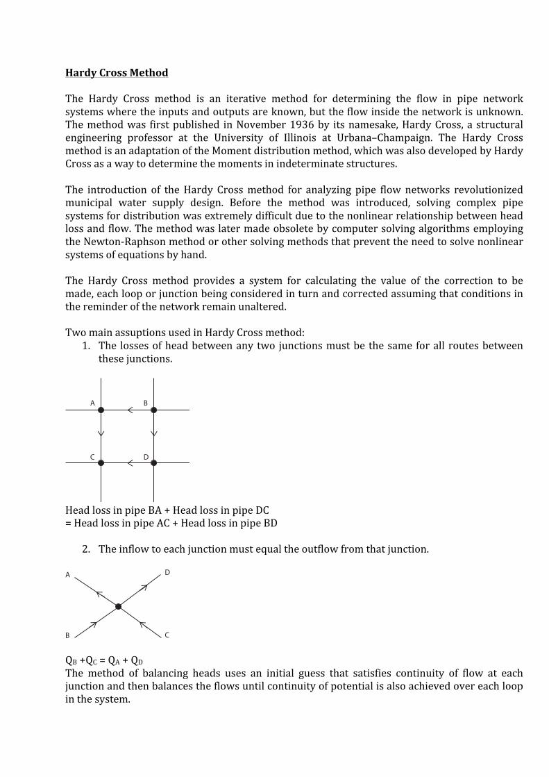
1. The   losses  of  head  between  any   two   junctions  must  be   the  same   for  all   routes  between  these  junctions.  

 

 Head  loss  in  pipe  BA  +  Head  loss  in  pipe  DC    =  Head  loss  in  pipe  AC  +  Head  loss  in  pipe  BD    

2. The  inflow  to  each  junction  must  equal  the  outflow  from  that  junction.    

   QB  +QC  =  QA  +  QD  The   method   of   balancing   heads   uses   an   initial   guess   that   satisfies   continuity   of   flow   at   each  junction  and  then  balances  the  flows  until  continuity  of  potential  is  also  achieved  over  each  loop  in  the  system.  

A B

C D

A

B C

D

 This   method   can   be   used   if   total   flow   rate   is   known.   Head   or   pressure   at   junctions   is   not  compulsory  item.    From  previous  lesson,  major  loss  can  be  determined  as:    

ℎ! = 𝑓 ∙𝐿𝐷 ∙

𝑉!

2𝑔 = 𝑓 ∙𝐿𝐷! ∙

162𝑔𝜋! ∙ 𝑄

! = 𝐾 ∙ 𝑄!  

 Head  loss  in  pipe  in  which  flow  is  clockwise;    

ℎ! = 𝐾! ∙ 𝑄!!    Head  loss  in  pipe  in  which  flow  is  counter-­‐clockwise;    

ℎ!! = 𝐾!! ∙ 𝑄!!!    Total  head  loss  is  constant,  whether  it  is  measured  clockwise  or  counter-­‐clockwise.    

𝐾! ∙ 𝑄!! = 𝐾!! ∙ 𝑄!!!      In  first  assumption,  we  assumed  that  the  losses  value  is  not  balanced.    

𝐾! ∙ (𝑄! − Δ𝑄)! = 𝐾!! ∙ (𝑄!! + Δ𝑄)!  

𝐾! ∙ (𝑄!! − 2𝑄! ∙ Δ𝑄 + Δ𝑄!) = 𝐾!! ∙ (𝑄!!! − 2𝑄!! ∙ Δ𝑄 + Δ𝑄!)    

Δ𝑄!  can  be  neglected.  Then,    

Δ𝑄 =𝐾! ∙ 𝑄!! − 𝐾!! ∙ 𝑄!!!

2( 𝐾! ∙ 𝑄! − 𝐾!! ∙ 𝑄!!)  

 It  is  known  that;    

ℎ! = 𝐾 ∙ 𝑄!  

𝐾 ∙ 𝑄 =ℎ!𝑄  

     Finally,      

Δ𝑄 =ℎ!" − ℎ!""

2(ℎ!"𝑄!

+ℎ!""𝑄!!

)  

   Calculation  will  be  done  many  times  until  the  value  of  ΔQ  is  approaching  zero.        

Example    Determine  the  distribution  of  flowrate?    

   Basic  step:  

1. Determine  loop  or  cycle.  2. Predict  the  initial  flow  rate  and  its  direction.  No  need  to  convert  unit  into  SI  unit.  3. Create  table  to  fulfill  the  Hardy  Cross  method  equation.  4. Redraw  the  figure,  and  propose  new  flow  rate.  ΔQ  value  is  not  the  answers.  5. Repeat  steps  1-­‐4  until  ΔQ  is  approaching  zero.  Propose  the  new  flow  rate.  

       

100 L/s

25 L/s

75 L/s

K=1

K=3

K=1

K=2

K=2

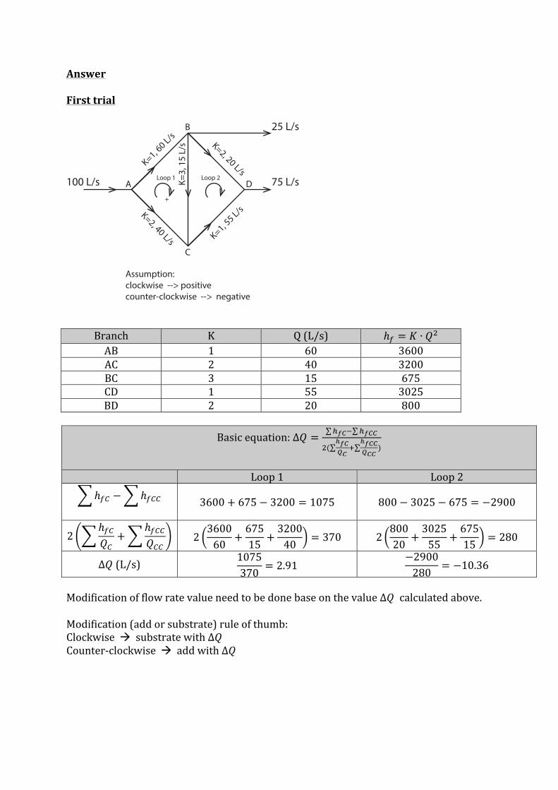
Answer    First  trial    

     

Branch   K   Q  (L/s)   ℎ! = 𝐾 ∙ 𝑄!  AB   1   60   3600  AC   2   40   3200  BC   3   15   675  CD   1   55   3025  BD   2   20   800  

 Basic  equation:  Δ𝑄 = !!"! !!""

!(!!"!!

!!!""!!!

)  

    Loop  1   Loop  2  

ℎ!" − ℎ!""    

3600+ 675− 3200 = 1075   800− 3025− 675 = −2900  

2ℎ!"𝑄!

+ℎ!""𝑄!!

  2360060 +

67515 +

320040 = 370   2

80020 +

302555 +

67515 = 280  

Δ𝑄  (L/s)   1075370 = 2.91  

−2900280 = −10.36  

 Modification  of  flow  rate  value  need  to  be  done  base  on  the  value  Δ𝑄    calculated  above.    Modification  (add  or  substrate)  rule  of  thumb:  Clockwise    à    substrate  with  Δ𝑄  Counter-­‐clockwise    à    add  with  Δ𝑄          

100 L/s

25 L/s

75 L/s

Assumption:clockwise --> positivecounter-clockwise --> negative

K=1, 60 L/s

K=2, 40 L/s

K=3,

15

L/s K=2, 20 L/s

K=1, 55 L/s

+Loop 1 Loop 2

+

A

B

C

D

Branch   Flow  direction   Loop   Δ𝑄   New  Q  (L/s)  AB   C  (  -­‐  )   1   2.91   60− 2.91 = 57.09  AC   CC  (  +  )   1   2.91   40+ 2.91 = 42.91  BC   C  (  -­‐  )  &  CC  (  +  )   1  &  2   2.91  &  -­‐10.36   15− 2.91+ (−10.36) = 1.73  CD   CC  (  +  )   2   -­‐10.36   55+ (−10.36) = 44.64  BD   C  (  -­‐  )   2   -­‐10.36   20− (−10.36) = 30.36  

 New  propose  flow  rate  and  its  direction  is:    

   However,   this   is   not   the   final   flow   rate,   because   the  Δ𝑄  is   still   shows   high   value.   Second   trial  calculation  need  to  be  done.  Repeat  the  procedure  until  the  value  of  Δ𝑄  is  almost  zero.            

100 L/s

25 L/s

75 L/s

57.09 L/s

42.91 L/s

1.73

L/s

30.36 L/s

44.64 L/s

A

B

C

D

Second  trial    Calculation  should  starts  with  this  flow  rate  value.    

           

100 L/s

25 L/s

75 L/s

57.09 L/s

42.91 L/s

1.73

L/s

30.36 L/s

44.64 L/s

A

B

C

D

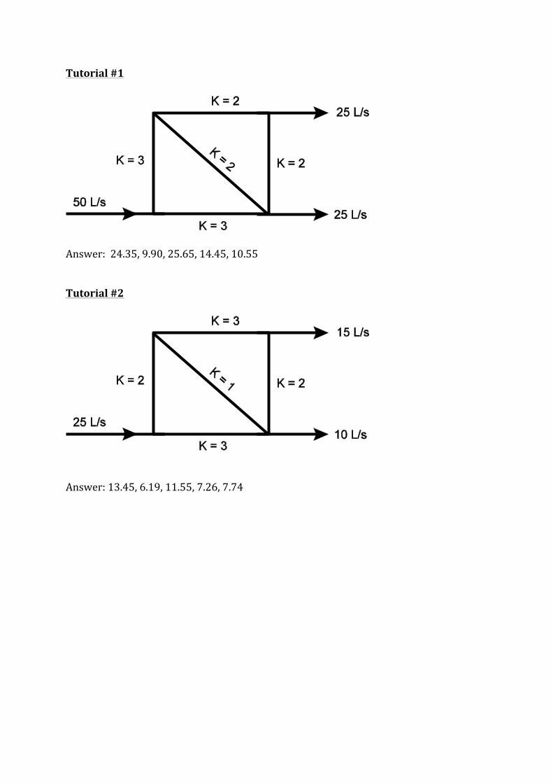
Tutorial  #1    

   Answer:    24.35,  9.90,  25.65,  14.45,  10.55      Tutorial  #2    

     Answer:  13.45,  6.19,  11.55,  7.26,  7.74