Rochester Institute of TechnologyRIT Scholar Works

Theses Thesis/Dissertation Collections

2-1-2010

Hardware co-processor to enable MIMO in nextgeneration wireless networksNathaniel Horner

Follow this and additional works at: http://scholarworks.rit.edu/theses

This Thesis is brought to you for free and open access by the Thesis/Dissertation Collections at RIT Scholar Works. It has been accepted for inclusionin Theses by an authorized administrator of RIT Scholar Works. For more information, please contact ritscholarworks@rit.edu.

Recommended CitationHorner, Nathaniel, "Hardware co-processor to enable MIMO in next generation wireless networks" (2010). Thesis. RochesterInstitute of Technology. Accessed from

Hardware Co-Processor to Enable MIMO inNext Generation Wireless Networks

by

Nathaniel Horner

A Thesis Submitted in Partial Fulfillment of the Requirements for the Degree of Master ofScience

in Computer Engineering

Supervised by

Professor Dr. Andres KwasinskiDepartment of Computer EngineeringKate Gleason College of Engineering

Rochester Institute of TechnologyRochester, New York

February 2010

Approved by:

Dr. Andres Kwasinski, ProfessorThesis Advisor, Department of Computer Engineering

Dr. Juan Cockburn, Associate ProfessorCommittee Member, Department of Computer Engineering

Dr. Shanchieh Yang, Associate ProfessorCommittee Member, Department of Computer Engineering

Thesis Release Permission Form

Rochester Institute of TechnologyKate Gleason College of Engineering

Title:

Hardware Co-Processor to Enable MIMO in Next Generation Wireless Networks

I, Nathaniel Horner, hereby grant permission to the Wallace Memorial Library to repro-duce my thesis in whole or part.

Nathaniel Horner

Date

iii

Acknowledgments

Id like to acknowledge Dr. Andres Kwasinski for his help and support throughout theresearch and experimentation of this thesis. Without his knowledge and experience within

the area of digital signal processors and wireless networking, this work would not havebeen possible. Id also like to thank and acknowledge Dr. Antonio F. Mondragon for

sharing his wisdom and experience within the area of hardware synthesis and design. Hisadvice and experience allowed the later parts of my experimentation to go much more

smoothly than anticipated.Id also like to thank my other committee members, Dr. Shanchieh Jay Yang and Dr. JuanCarlos Cockburn, for their patience and advice throughout this process. Finally, Id like to

thank my classmates within the Department of Computer Engineering, especially mycolleges in the NetIP Lab, particularly Daniel Stella, Daniel Liu, Chris Murphy, Jordan

Bean, Athena Frazier, Kheim Tong and Xander Fiss for their input, advice and perspectiveon my research and presentations.

iv

AbstractHardware Co-Processor to Enable MIMO in Next Generation Wireless Networks

Nathaniel Horner

Supervising Professor: Dr. Andres Kwasinski

One prevailing technology in wireless communication is Multiple Input, Multiple Output

(MIMO) communication. MIMO communication simultaneously transmits several data

streams, each from their own antenna within the same frequency channel. This technique

can increase data bandwidth by up to a factor of the number of transmitting antennas, but

comes with the cost of a much higher computational complexity for the wireless receiver.

MIMO communication exploits differing channel effects caused by physical distances

between antennas to differentiate between transmitting antennas, an intrinsically two di-

mensional operation. Current Digital Signal Processors (DSPs), on the other hand, are

designed to perform computations on one dimensional vectors of incoming data. To com-

pensate for the lack of native support of these higher dimensional operations, current base

stations are forced to add multiple new processing elements while many mobile devices

cannot support MIMO communication. In order to allow wireless clients and stations to

have native support of the two dimensional operations required by MIMO communication,

a hardware co-processor was designed to allow the DSP to offload these operations onto

another processor to reduce computation time.

v

Contents

Acknowledgments . . . . . . . . . . . . . . . . . . . . . . . . . . . . . . . . . iii

Abstract . . . . . . . . . . . . . . . . . . . . . . . . . . . . . . . . . . . . . . . iv

1 Introduction . . . . . . . . . . . . . . . . . . . . . . . . . . . . . . . . . . . 1

2 Overview of MIMO Communication . . . . . . . . . . . . . . . . . . . . . 42.1 General Overview . . . . . . . . . . . . . . . . . . . . . . . . . . . . . . . 42.2 MIMO Transmission . . . . . . . . . . . . . . . . . . . . . . . . . . . . . 62.3 Orthogonal Frequency Division Multiplexing . . . . . . . . . . . . . . . . 92.4 MIMO Signal Detection . . . . . . . . . . . . . . . . . . . . . . . . . . . 12

3 Methodology . . . . . . . . . . . . . . . . . . . . . . . . . . . . . . . . . . 193.1 Targeted Algorithms for Calculating the MMSE Pseudo-Inverse . . . . . . 193.2 Typical and Targeted DSP Architectures . . . . . . . . . . . . . . . . . . . 233.3 Creation of a DSP-Only Baseline for Comparison . . . . . . . . . . . . . . 253.4 New Intrinsic Operations . . . . . . . . . . . . . . . . . . . . . . . . . . . 263.5 Creation of a DSP and Co-Processor Implementation . . . . . . . . . . . . 27

3.5.1 Targeted Pipeline and Initial Stage . . . . . . . . . . . . . . . . . . 283.5.2 ASIC Stages . . . . . . . . . . . . . . . . . . . . . . . . . . . . . 29

4 Results . . . . . . . . . . . . . . . . . . . . . . . . . . . . . . . . . . . . . . 374.1 Determining Baseline Cycles . . . . . . . . . . . . . . . . . . . . . . . . . 374.2 Determining DSP Pre-process Cycles for Co-processor Implementations . . 384.3 Determining Cycles spent on ASIC for Co-processor Implementations . . . 39

5 Conclusions and Future Work . . . . . . . . . . . . . . . . . . . . . . . . . 43

Bibliography . . . . . . . . . . . . . . . . . . . . . . . . . . . . . . . . . . . . 44

A Base DSP Householder Implementation Code and Test Wrapper . . . . . . 47

vi

B Base DSP Greville Implementation Code and File Test Wrapper . . . . . . 48

C Test Matrices . . . . . . . . . . . . . . . . . . . . . . . . . . . . . . . . . . 49

D Modified SimpleScalar Code . . . . . . . . . . . . . . . . . . . . . . . . . . 50

E DSP and Co-processor Householder DSP Code . . . . . . . . . . . . . . . . 51

F DSP and Co-processor Greville DSP Code . . . . . . . . . . . . . . . . . . 52

G DSP and Co-processor Householder ASIC Column Processor Code . . . . . 53

H DSP and Co-processor Greville ASIC Row Processor Code . . . . . . . . . 54

vii

List of Figures

2.1 Multipath effects in SISO wireless communication. . . . . . . . . . . . . . 52.2 MIMO 3 transmitter, 4 receiver channel model. . . . . . . . . . . . . . . . 72.3 OFDM signal formation (top) and reconstruction (bottom). . . . . . . . . . 102.4 Division of a channel’s amplitude (top) and phase (bottom) frequency re-

sponse (black) into discrete sub-channels (gray). . . . . . . . . . . . . . . . 112.5 Pilot symbol location defined in IEEE 802.16e [7]. . . . . . . . . . . . . . 122.6 Simple Sphere Detector example. . . . . . . . . . . . . . . . . . . . . . . . 18

3.1 Block diagram of Householder algorithm. . . . . . . . . . . . . . . . . . . 213.2 Block diagram of Greville algorithm [16]. . . . . . . . . . . . . . . . . . . 223.3 Bit errors for every element of the matrix after two, three, and four itera-

tions of the main loop in the Greville method. . . . . . . . . . . . . . . . . 313.4 Processing locations of Householder block diagram. . . . . . . . . . . . . . 323.5 Processing locations of Greville block diagram. . . . . . . . . . . . . . . . 333.6 Pipeline concept for DSP and ASIC computation. . . . . . . . . . . . . . . 343.7 Communication between DSP and Co-processor via shared buffer. . . . . . 353.8 Pipeline showing delay on read for matrix processing. . . . . . . . . . . . . 353.9 General flow for C-Code to RTL in PICO [4]. . . . . . . . . . . . . . . . . 363.10 Data flow between DSP and ASICs in FIFOs. . . . . . . . . . . . . . . . . 36

4.1 Screenshot of PICO included files and implementation setup. . . . . . . . . 404.2 Speedup vs. Estimated Area for Householder implementation. . . . . . . . 414.3 Speedup vs. Estimated Area for Greville implementation. . . . . . . . . . . 42

1

Chapter 1

Introduction

The maximum data rate of a wireless signal is determined by both the encoding scheme

and the frequency bandwidth of the medium in which the information is transmitted. En-

hancements in both architecture and technology have increased the computational power of

signal processors which have, in turn, increased the allowable complexity of the encoding

schemes. The available transmission spectrum, on the other hand, is auctioned by the FCC

in fixed channels. The use of modified auction formats to reduce collusion between buyers

as well as increased demand for wireless channels has driven the cost of spectral licenses to

prohibitively high levels [11]. Therefore, due to ever-increasing computational resources

and a fairly fixed transmission spectrum, it is advantageous to utilize more computationally

complex wireless transmission schemes in order to achieve higher spectral efficiency.

Toward this end, Multiple-Input Multiple-Output (MIMO) communication has been in-

troduced in the main wireless communication standards as a method to achieve higher spec-

tral efficiency. In MIMO communication multiple antennas transmit information to mul-

tiple antennas on one receiver. Under ideal circumstances, if the information transmitted

by each individual antenna could be differentiated and fully recovered, this could increase

the spectral efficiency by a factor of the number of transmitting antennas. The signal pro-

cessing required for differentiating between different transmitting antennas and recovering

each transmitter’s information increases the required computations significantly, producing

a higher data rate signal at the cost of higher computational complexity [13]. Many new

2

wireless protocols include the use of MIMO communication [2][7][3], but these protocols

are implemented on top of hardware designed towards Single-Input, Single-Output (SISO)

communication. Some devices, such as wireless routers, can perform this computationally

expensive communication due to high resources including DSPs or FPGAs dedicated to

MIMO operations and can currently use the IEEE 802.11n protocol which allows for be-

tween two and four transmit and receive antennas [2]. Current common implementations

use only two transmit and receive antennas due to a much lower computational complexity.

Another widely-used standard that is adopting MIMO technology is the Long Term

Evolution (LTE) standard. With the goal of providing highly-mobile broadband connec-

tions, LTE will use many new techniques to improve down-link and up-link speeds. The

primary use of MIMO discussed in this work is to broadcast different data streams from

different antennas simultaneously and use the spatial differences between the antennas to

differentiate between broadcast streams at the receiver. Like IEEE 802.11n, LTE allows for

two and four transmitting and receiving antennas [3].

The primary drawback associated with all MIMO protocols is the computation cost.

The maximum data rate is strongly related to the number of transmission or receiver an-

tennas [20], but the addition of further antennas greatly increases the number of operations

required to reconstruct the signal [13]. The receiver must model the wireless channel by

estimating each transmitting antenna’s effect on each receiver antenna, forming a matrix.

The operations involved in estimating the transmitted signal using this channel model are

therefore intrinsically matrix operations. Current hardware is designed for vector-based op-

erations associated with single-input, single-output communication, and cannot efficiently

compute the matrix operations required in MIMO communication. Current MIMO devices

compensate for this lack of efficiency by adding more processing elements, an approach

that increases cost and power requirements. In platforms where adding additional process-

ing elements is not an option, such as cell phones and other mobile devices, the current

3

processing power is insufficient to implement MIMO methods of communication. Enhanc-

ing hardware to provide native support for these matrix operations is a preferable solution

for devices that are currently modified with additional processing elements, and required

for other devices which cannot support additional processing elements.

4

Chapter 2

Overview of MIMO Communication

2.1 General Overview

SISO wireless communication over a single frequency transmits data by phase and/or am-

plitude encoding, i.e. different phase and amplitude combinations in the transmitted signal

correspond to different bit values in the digital signal [13]. This amplitude and phase com-

bination of the transmitted signal can be represented by a complex number, x. The medium

through which the signal is transmitted will have power loss (affecting the amplitude) and

delay elements (affecting the phase) that will change the transmitted signal. Assuming that

the channel will have constant amplitude and phase effects across all frequencies within the

channel, these amplitude and phase effects from the channel can be represented as a second

complex number, Γ . Background noise in the medium combined with any noise within the

transmitter and receiver is typically modeled as Additive White Gaussian Noise (AWGN),

which is added to the product of the channel effects and original transmitted signal, form-

ing the received signal, y, as shown in Eq. (2.1), with corresponding signal to noise ratio

(SNR), γ, in Eq. (2.2).

y = Γx+ n (2.1)

γ =|Γ|n

(2.2)

The SISO approach relies heavily upon receiving one strong signal from the transmitter

5

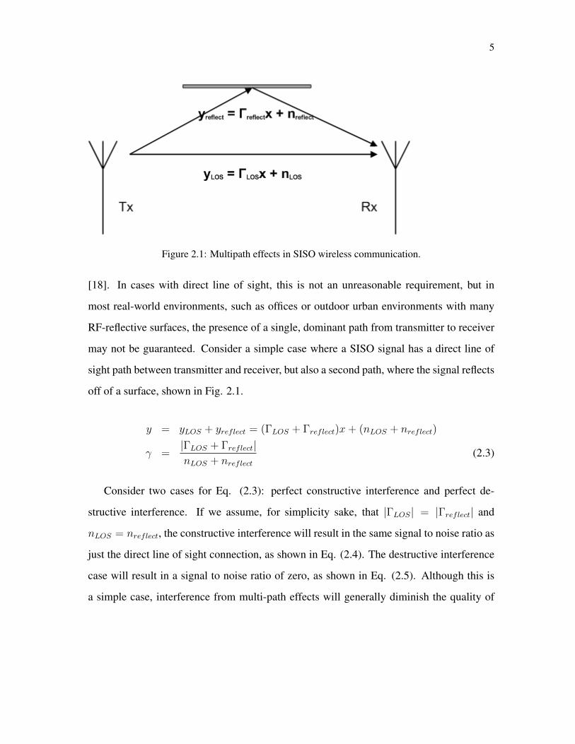
Figure 2.1: Multipath effects in SISO wireless communication.

[18]. In cases with direct line of sight, this is not an unreasonable requirement, but in

most real-world environments, such as offices or outdoor urban environments with many

RF-reflective surfaces, the presence of a single, dominant path from transmitter to receiver

may not be guaranteed. Consider a simple case where a SISO signal has a direct line of

sight path between transmitter and receiver, but also a second path, where the signal reflects

off of a surface, shown in Fig. 2.1.

y = yLOS + yreflect = (ΓLOS + Γreflect)x+ (nLOS + nreflect)

γ =|ΓLOS + Γreflect|nLOS + nreflect

(2.3)

Consider two cases for Eq. (2.3): perfect constructive interference and perfect de-

structive interference. If we assume, for simplicity sake, that |ΓLOS| = |Γreflect| and

nLOS = nreflect, the constructive interference will result in the same signal to noise ratio as

just the direct line of sight connection, as shown in Eq. (2.4). The destructive interference

case will result in a signal to noise ratio of zero, as shown in Eq. (2.5). Although this is

a simple case, interference from multi-path effects will generally diminish the quality of

6

SISO wireless signals.

γ =|ΓLOS + Γreflect|nLOS + nreflect

=2 |ΓLOS|2nLOS

=|ΓLOS|nLOS

= γLOS (2.4)

γ =|ΓLOS + Γreflect|nLOS + nreflect

=|ΓLOS| − |ΓLOS|

2nLOS=

0

nLOS= 0 (2.5)

MIMO communication, involving multiple transmit and multiple receive antennas as

shown in Fig. 2.2, can provide a more robust, higher data rate signal in environments with

multi-path effects [20]. If the transmitting and receiving antennas are sufficiently far apart

in terms of the signal wavelength, λ (for example, 8 cm ≈ λ/2 for a 1.9 GHz signal), the

channel between the transmitting and receiving antennas can be assumed to be sufficiently

different. For the multi-path example given in the SISO case, the delay from the reflected

signal would be different for each receiving antenna, making destructive interference for

both receivers much less likely.

From an alternative, higher level view, if the channel has a 50% probability of being

down for any data stream, a SISO connection will only achieve 50% of its maximum data

rate, as half of the information will be lost. A MIMO scheme with two data streams trans-

mitting the same information can achieve a 25% failure rate, as the probability of both data

streams failing at the same time is 0.5 * 0.5, or 25%. If the MIMO scheme were transmit-

ting different information from two different data streams simultaneously and it is assumed

that the receiver is able to differentiate between the two streams and recover them inde-

pendently, each stream will achieve 50% of its maximum data rate (as in the SISO case),

leading to twice the data rate of the SISO case, as there are two transmitting streams.

2.2 MIMO Transmission

Under MIMO schemes, each transmitting antenna can transmit independent information

from the other transmit antennas. At any given time, the symbols being broadcast can be

7

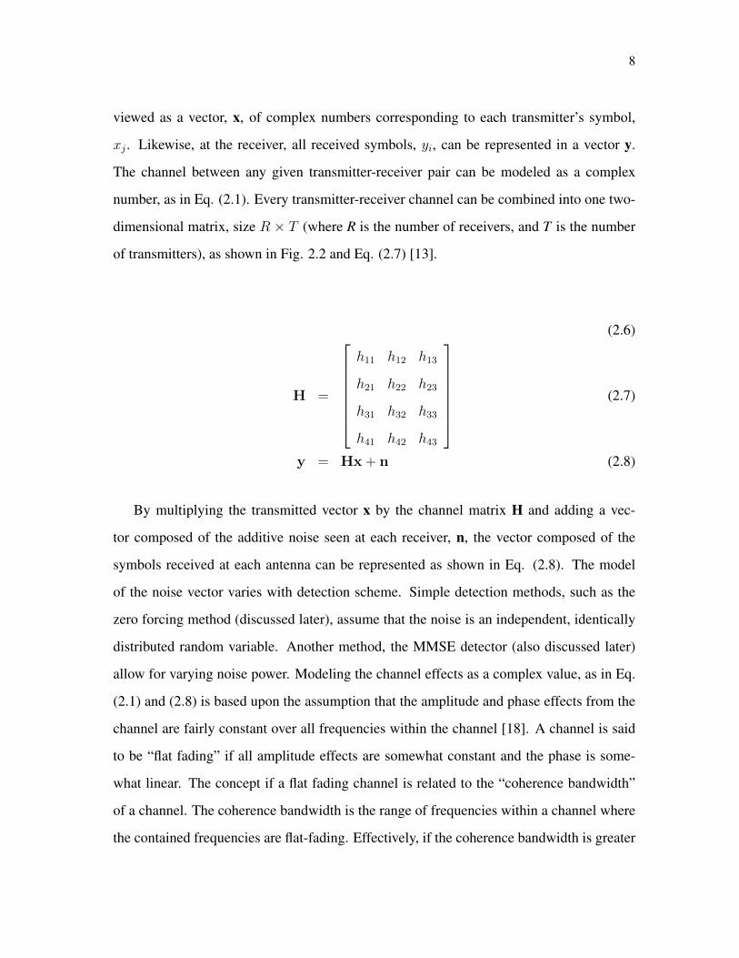
Figure 2.2: MIMO 3 transmitter, 4 receiver channel model.

8

viewed as a vector, x, of complex numbers corresponding to each transmitter’s symbol,

xj . Likewise, at the receiver, all received symbols, yi, can be represented in a vector y.

The channel between any given transmitter-receiver pair can be modeled as a complex

number, as in Eq. (2.1). Every transmitter-receiver channel can be combined into one two-

dimensional matrix, size R × T (where R is the number of receivers, and T is the number

of transmitters), as shown in Fig. 2.2 and Eq. (2.7) [13].

(2.6)

H =

h11 h12 h13

h21 h22 h23

h31 h32 h33

h41 h42 h43

(2.7)

y = Hx + n (2.8)

By multiplying the transmitted vector x by the channel matrix H and adding a vec-

tor composed of the additive noise seen at each receiver, n, the vector composed of the

symbols received at each antenna can be represented as shown in Eq. (2.8). The model

of the noise vector varies with detection scheme. Simple detection methods, such as the

zero forcing method (discussed later), assume that the noise is an independent, identically

distributed random variable. Another method, the MMSE detector (also discussed later)

allow for varying noise power. Modeling the channel effects as a complex value, as in Eq.

(2.1) and (2.8) is based upon the assumption that the amplitude and phase effects from the

channel are fairly constant over all frequencies within the channel [18]. A channel is said

to be “flat fading” if all amplitude effects are somewhat constant and the phase is some-

what linear. The concept if a flat fading channel is related to the “coherence bandwidth”

of a channel. The coherence bandwidth is the range of frequencies within a channel where

the contained frequencies are flat-fading. Effectively, if the coherence bandwidth is greater

9

than the channel bandwidth, the channel can be approximated as a complex value. If the

coherence bandwidth is less than the channel bandwidth, it is not safe to model the channel

as a complex value. In practice, the channel will act as a filter, with amplitude and phase

effects changing as a function of frequency and modeling the channel as a single complex

value is not safe. By dividing the transmission channel into many independent narrow-band

sub-channels, the frequency and phase response can be assumed to be somewhat constant

within any individual sub channel. This division into many sub-channels can be accom-

plished through the method of Orthogonal Frequency Division Multiplexing (OFDM) [10].

2.3 Orthogonal Frequency Division Multiplexing

OFDM transmits a series of symbols in parallel, each over their own narrow bandwidth

sub-channel within the main channel. With schemes prior to OFDM, higher data rates

were achieved by reducing the time taken to transmit each symbol in serial. With OFDM,

many symbols are transmitted in parallel over a much longer period of time. Each symbol

is encoded to an amplitude/phase complex value, dk, using a standard method, such as

quadrature amplitude modulation (QAM) [13]. These symbols are all modulated with their

own sub-channel frequency, fk, which is calculated from a base frequency, f1 and the

frequency spacing, ∆k, as shown in Eq. (2.9). These symbols dk and frequencies fk can

then be combined to form one OFDM symbol, s as shown in Eq. (2.10).

fk = f1 + (k − 1) ∗∆k (2.9)

s(t) =K∑k=1

dkej2πfkt (2.10)

The OFDM symbol formation operation can be expressed as a superposition of the

input symbols d at their respective frequencies, fk. By forcing f1 = 0, Eq. (2.10) can be

expressed as taking the inverse Fourier transform of the input signal d. This low-frequency

signal can then be modulated with the carrier frequency for transmission, as shown in Fig.

10

2.3 [10].

Figure 2.3: OFDM signal formation (top) and reconstruction (bottom).

After formation of the signal, a prefix is added before transmission. The last L samples

of the signal s(t) are added before the signal. This produces a final signal in Eq. (2.11),

where K is the length of the signal s(t), giving s(t), a signal of length of K + L. This cyclic

prefix allows the channel to account for different delays within a multi-path environment,

where the previous symbols arriving from longer delay paths could interfere with succes-

sive symbols arriving on shorter delay paths [23]. The interference between these symbols

is not included within the channel model in Eq. (2.8). Because of the delay from the prefix,

most multi-path effects will dissipate before the actual symbol starts transmission [18].

s(t) = [sK−L+1, sK−L+2, ...sK−1, s0, s1, ...sK−2, sK−1] (2.11)

To recover the original vector of sub-symbols, the signal must be demodulated about the

carrier and the cyclic prefix removed. Taking the Fourier Transform of this resulting signal

will produce the original symbol vector with amplitude, phase modulations and noise from

11

Figure 2.4: Division of a channel’s amplitude (top) and phase (bottom) frequency response (black)into discrete sub-channels (gray).

the channel. Because each sub-symbol is only transmitted within its own sub-channel (and

there is nearly no overlap between channels), channel effects for each sub-channel can be

modeled individually. Division of the channel into many small subchannels makes it much

safer to assume that the coherence bandwidth is greater than the sub-channel bandwidth as

shown in Fig. 2.4 [18]. This safety is not without additional cost: dividing the channel into

many sub-channels requires that channel estimation and symbol detection be performed

for each sub-channel, increasing computational complexity by a factor of the number of

OFDM sub-channels. In the case of MIMO communication, each sub-channel must be

estimated and the inverse of each sub-channel estimate calculated. Currently, the IEEE

802.11n protocol allows for up to 256 OFDM sub channels at the mobile client for every

channel, increasing complexity by a factor of 256 in addition to the signal conditioning

outlined in Fig. 2.3 [2]. Base station units can communicate with several clients in adjacent

12

channels, creating potential thousands of OFDM sub channels.

2.4 MIMO Signal Detection

After the symbol is broken into sub-symbols and transmitted over the channel via OFDM,

it must be reconstructed back into an estimate of the transmitted symbol. In order to create

this symbol estimate, the channel matrix H must first be estimated. Symbols known both

to the transmitter and receiver, known as “pilot” or “reference” symbols, are periodically

transmitted during communication and used to solve for the channel matrix H [22][15].

The OFDM sub-channel, transmission time, and value of these symbols are defined in each

wireless protocol. The channel estimate is formed at the receiver by methods also defined

by each individual protocol.

Figure 2.5: Pilot symbol location defined in IEEE 802.16e [7].

These pilot symbols are an orthogonal set of symbols broadcast from each transmit

antenna with known power to provide an estimate of the power loss from the channel. In

13

order to provide an estimate of the channel phase, these symbols also typically have Zero

Auto-Correlation (ZAC) to allow the receiver to quickly determine the delay effects [19]. In

both WIMAX and LTE (among others), these pilot symbols are only sent in certain OFDM

sub-channels [3]. A typical mapping of these pilot blocks in both frequency and time is

shown in Fig. 2.5. The channel estimation is first formed for these pilot channel blocks

and then typical interpolation methods, such as linear or mean squared error, are used to

estimate the intermediate channel blocks [15].

Using an estimate of the channel matrix, the transmitted symbol can be subsequently

estimated via some detection algorithm that will determine the symbol that was most likely

transmitted given the received symbol and the channel matrix. The optimal detector is the

maximum likelihood (ML) detector which determines the candidate symbol vector from

the space of all possible symbol vectors which has the greatest likelihood of being the

transmitted vector. The ML detector compares the received symbol to the symbol produced

by multiplying the channel matrix by each possible transmitted symbol, ci, and choosing

the candidate symbol with the lowest mean squared error from the received signal, c,as

shown in Eq. (2.12) [17].

c = arg minc∈C ‖y −Hc‖ (2.12)

The detector in Eq. (2.12) is not feasible for many applications, as it requires each

possible symbol vector be multiplied by a channel matrix every time the channel matrix

is estimated followed by an exhaustive search of every resulting product for every symbol

received in order to identify the symbol with the maximum likelihood of having been sent.

If there are T transmitters and Q bits per symbol transmitted from each receiver, there are

2TQ possible combinations, and therefore the detector in Eq. (2.12) would require 2TQ

matrix-vector multiplications and then computation of 2TQ mean squared errors. Even in a

simple case of T = 2 and Q = 3 with 256 OFDM sub-channels, the resulting 16384 matrix-

vector multiplications per channel estimate and 16384 mean squared error calculations per

14

symbol is not computationally feasible [17].

Different detectors have been proposed to approximate the ideal detector in Eq. (2.12)

while remaining less computationally complex. A simple and naive approach is to simply

solve for x in Eq. (2.8) ignoring the noise, n [17]. This estimate requires finding the inverse

of the channel matrix H and multiplying this inverse by the received vector y to produce an

estimate of c, c, as shown in Eq. (2.13).

c = H−1y (2.13)

This detector is called a Zero-Forcing detector (ZF) [25] because of its method to force

any effects from other transmitting antennas to zero in order to differentiate each transmit-

ting antenna. To determine the output vector from c in Eq. (2.13), each element of c is

individually compared to the set of possible symbols for that particular index, Ck, and the

resulting output vector, c, is composed of the individual lowest error candidates for each

element, as shown in Eq. (2.14), where ck represents the kth element of the estimate vector,

determined in Eq. (2.13).

ck = arg minci∈Ck|ci − ck| (2.14)

The first issue in the implementation of a ZF detector is the computation of the matrix

inverse in Eq. (2.13). While the size of the channel matrix will be relatively small (current

protocols allow for up to 4x4 matrices), this inversion must be repeated once per OFDM

sub channel. QR (or QL) decomposition [14][9] has been applied as a substitute for direct

computation of the inverse as it allows application of H−1 while remaining less compu-

tationally complex than matrix inversion [14]. QR decomposition represents the channel

matrix as the product of two matrices, an orthonormal matrix, Q and an upper triangular

matrix R, as shown in Eq. (2.15). By substituting H for QR, and using the matrix identity

15

that (AB)−1 = B−1A−1, we obtain Eq. (2.16).

QR = H (2.15)

QQH = QHQ = I

c = (QR)−1y = R−1QHy (2.16)

Observe that, in the case where H is a 4x3 matrix, R is of the form

R =

r11 r12 r13

0 r22 r23

0 0 r33

0 0 0

Let y = QHy

c3 = r−133 y3, therefore

c3 =y3r33

using this value of c3 to solve for c2,

c2 =y3 − r23c3

r22(2.17)

Using Eq. (2.17) (with the numerator expanding to use every previously calculated

element of c), one can solve for every element of c without directly calculating a matrix

inverse. A variant of the ZF detector, the Zero Forcing detector with Decision Feedback

(ZF-DF) [17] has also been proposed which first calculates an element ck and then imme-

diately calculates the minimum error symbol estimate, cZF−DFk. Instead of then using ck

to calculate the next element in c, it incorporates the minimum error decision and uses the

actual output symbol value for further calculations, shown below in Eq. (2.18).

c3 =y3r33

cZF−DF3 = arg minci∈C3|ci − c3|

16

c2 =y3 − r23cZF−DF3

r22(2.18)

Both the ZF and ZF-DF detectors have error rates higher than the optimal ML detector.

The primary problems are that they ignore any additive noise present in the channel and

at the receiver and that they assume that an inverse (or decomposition) of the channel

matrix exists. In cases where the number of transmit antennas is greater than the number of

receivers, this inverse will not exist. Introducing another, more robust, method of inverting

the channel matrix, the Minimum Mean-Squared Error (MMSE) Moor-Penrose Pseudo

Inverse, as show in Eq. (2.19), minimizes E[∥∥H†y − c

∥∥], where D is a diagonal matrix of

the inverse of the Signal-to-Noise ratio, hereby referred to as the Noise-to-Signal ratio, of

each transmitting antenna and H† is the MMSE Pseudo Inverse.

H† =(HHH + D2

)−1HH (2.19)

The same methods to determine the output vector as the ZF and ZF-DF methods, shown

in Eq. (2.17) and (2.18) can be used with the MMSE detector. To apply to the ZF and ZF-

DF methods, (HHH + D2) would be decomposed into QR and y would equal QHHHy,

as shown in Eq. (2.20) and (2.21). Using the MMSE inverse requires added complexity

to calculate HHH + D2, but produces a more robust, more accurate detector by ensuring

both that the additive noise is included in the calculation and that the matrix inversion is

performed upon a matrix of suitable size (the inverted portion is a TxT square matrix) [25].

QR = (HH + D2) (2.20)

c = (QR)−1HHy

c = R−1Q−1HHy = R−1QHHHy (2.21)

An alternative to the ZF and ZF-DF detectors is the Sphere Detector (SD) [24]. While

17

the ZF and ZF-DF detectors determine one element of the output vector at a time, based

either on the equalizer matrix or on both the matrix and the previously determined elements

of the output vector, the SD performs a tree search through all possible transmitted vectors

and keeps track of the error for any particular path. If the error for a path exceeds some

specified threshold, referred to as the “radius,” the SD abandons the branch. It then chooses

the path with the lowest total summed error. A simple example of a SD with radius = 1 and

four transmitters is shown in 2.6. The search works as follows: first, a value of c1 = 0 is

attempted. This produces an error of 0.8, which is below the radius, so the search continues.

No values of c2 produce an error lower than the radius, however, so the path is abandoned.

A value of c1 = 1 produces an error within the radius, so the search expands this node.

The search continues on, expanding nodes that produce an error within the radius, until all

paths are searched. In this case, only one path reaches the end of the search.

One advantage to the SD is that once a path is found that reaches a terminal node in the

tree, in other words forming a full estimate vector, the maximum radius can be lowered to

the summed error of this path, as the final estimate vector will have at most the same error

as the current minimum path[17]. The estimate vector c can be determined via either a ZF

or MMSE detection method.

The disadvantage of the SD is that it does not have a fixed computation time. Depending

on the radius, it can implement the optimal detector in Eq. (2.12), and it is possible that it

will not return any output if there is no path within the search radius. The second problem

may be desirable in practice, as any vector outside of the radius is likely erroneous.

Many other detectors have been proposed with the goal of achieving a lower bit er-

ror rate than these detectors. These detectors, however, typically ignore the computational

complexity of the proposed method and instead focus on a comparison of error rate. Fur-

thermore, many of these detectors target a specific wireless protocol and seek to exploit

particular elements of the protocol, such as specific amplitude-phase encoding techniques.

As this work is intended to target a more general solution, independent of protocol and

18

Figure 2.6: Simple Sphere Detector example.

focusing on feasible implementations, these detectors have not been included in this inves-

tigation.

19

Chapter 3

Methodology

The main drawback of MIMO communication, as discussed previously, is that it greatly

increases the computational complexity of signal reconstruction for both the transmitter

and receiver. Mobile clients (such as laptops, cell phones, etc) have not been designed

to natively support the matrix-type operations required and may not have a high amount

of resources available to fully implement current and future MIMO wireless protocols.

Currently, resource restrictions are limiting the number of transmit/receive antennas and

limiting the performance of the symbol detection algorithms for mobile clients. On the

base-station side, more signal processors are being added at a higher cost in order to cope

with the higher complexity of signal formation and detection. In order to better support

these matrix operations, current hardware must be enhanced to incorporate these required

operations at the design level to fully support current and future MIMO communication

requirements.

3.1 Targeted Algorithms for Calculating the MMSE Pseudo-Inverse

The MMSE detector was chosen as the detector of choice, as it fully utilizes channel infor-

mation and can be used in situations where the matrix inversion of a ZF detector would not

be possible, such as situations with a higher number of transmit than receive antennas [8].

In order to examine the requirements of hardware support without targeting any specific

20

algorithm or method, two different methods for calculating the pseudo-inverse were cho-

sen: a Householder Q-R decomposition-based algorithm that would output two matrices

for a given channel matrix and noise-to-signal ratio vector, and a modified version of the

Greville method of direct computation for the matrix pseudo-inverse [16]. Pseudo code for

each of these algorithms is shown below, with block diagrams in Fig. 3.1 and Fig. 3.2.

Householder Decomposition Algorithm1. R← HH ∗H2. Q← HH

3. for(col = 1 : N)

4. z ← R[col : N, col]

5. b← sqrt(zH ∗ z)

6. z[1]← z[1]− b7. b← 1/(b ∗ z[1])

8. zR ← zH ∗R[col : N, col : N ]

9. zQ ← zH ∗Q[col : N, 1 : M ]

10. z ← z ∗ b11. R[col : N, col : N ]← R[col : N, col : N ] + zR ∗ z12. Q[col : N, 1 : M ]← Q[col : N, 1 : M ] + zQ ∗ z13.end for

Novel Greville Algorithm1. a← D[1, 1]2 +H[1 : M, 1]H ∗H[1 : M, 1]

2. G[1, 1 : M ]← H[1 : M, 1]H/a

3. for(k = 2 : N)

4. v ← G[1 : k − 1, 1 : M ] ∗H[1 : M,k]

5. G[k, 1 : M ]← H[1 : M,k]H − vH ∗H[1 : M, 1 : k − 1]H

6. a← D[k, k]2 + real(G[k, 1 : M ] ∗H[1 : M,k])

7. G[k, 1 : M ]← G[k, 1 : M ]/a

8. G[1 : k − 1, 1 : M ]← G[1 : k − 1, 1 : M ]− v ∗G[k, 1 : M ]

9. end for

These two particular algorithms were chosen to provide a representation of different

pseudo-inverse methods available. They both use atomic matrix operations, such as matrix

21

Figure 3.1: Block diagram of Householder algorithm.

22

Figure 3.2: Block diagram of Greville algorithm [16].

vector multiplication and vector inner and outer products, but their methods are very differ-

ent. The method of Greville processes one row at a time, while Householder decomposition

processes by column. The dimensions are also different: the Greville method involves more

operations with each iteration of the main loop: it processes the first row, then the first two,

then the first three and so on, while the Householder method starts by examining the entire

matrix, then removing the first row and column, then the second, reducing complexity with

23

each iteration. Some atomic operations are also different. For example, the Householder

decomposition includes a normalization requiring a square root operation, while the Gre-

ville method requires use of dot products to calculate a real portion of a multiplication. In

terms of performance, the Greville method was expected to outperform the Householder

decomposition, due to its lower numbers of multiply operations and the fact that it uses

mainly fixed-length vectors, which are better implemented on DSPs [16].

To better examine how these algorithms would perform on a Digital Signal Processor

(DSP) in order to form a baseline for comparison, code was written with channel elements

as fixed-point 32-bit complex values (16-bit real, 16-bit complex, 8 decimal bits). For

this code, it was assumed that the number of receiving antennas would be fixed (as this is

a hardware aspect of the receiving device), but the number of transmitting devices could

vary between two and four to allow for use in different transmitting devices or allow for

the case where a transmitting antenna is not detected at the receiver.

3.2 Typical and Targeted DSP Architectures

Typical DSPs are designed to handle many algorithms specific to signals processing, such

as FIR filtering or the Fast Fourier Transform. To deal with typically high amounts of com-

putations required for data sets, DSP architectures tend to be capable of high levels of paral-

lel computation and arithmetic units designed specifically for required operations, mainly

multiply and accumulate operations. Many DSPs lack general functionality provided by

many microprocessors, as they may not include support of floating point, division, square

root, or exponential operations. There are operations specific to DSPs, however, which

are added to allow fast computation of specific algorithms. For example, there are bit

reversal operations in most DSPs which allow for faster computation of addresses in the

Fast Fourier Transform and there are saturated arithmetic operations to prevent overflow on

digital signals [12].

Because of their fast, relatively low cost computation capabilities, the use of DSPs has

24

expanded from traditional roles, such as radio communication and audio conditioning, to

include many new roles, such as media processing (audio/video decoding) and encryp-

tion/decryption operations. When possible, DSPs are modified to fit these new roles by

addition of new operations in the instruction set. The operations required, however, are not

always compatible with DSP architectures. To add support for these new operations, some

DSP cores are augmented with additional programmable co-processors which are specifi-

cally designed for these operations. For example, the Texas Instruments DM6467T digital

media processor includes a hardware co-processor that can quickly compute decode oper-

ations (such as the discrete cosine transform) required of video decoding methods such as

H.264 and MPEG4 at 60 frames per second [5].

The targeted DSP for this work is the Texas Instruments C64x+ DSP [1]. A member of

the TI TMS320 family, this DSP includes eight total operational units, with pairs targeted

towards different types of instructions, and two banks of 32 32-bit registers. It has opera-

tions capable of working with 8, 16, 32, 40, and 64-bit operands and/or outputs, with 40

and 64-bit operands/outputs implemented on two adjacent 32-bit registers. This platform

was chosen for its high computational capability as well as the C6400 familys wide use

in industry. Its instruction set includes a four-cycle complex multiply, round and shift op-

eration as well as native support of pairs of 16-bit values (real and complex) packed into

32-bit registers. Software for this DSP can be developed in TIs Code Composer Studio

(CCS) which allows for development and simulation and program profiling to measure ac-

curate cycle counts spent in specific ranges or functions. The CCS profiling tool was one

of the tools used to gather metrics for program run-times. Another benefit of CCS is the

compilers use of intrinsic operations. Intrinsic operations allow a developer to use a spe-

cific operation in the DSPs instruction set, such as a complex multiply operation. These

intrinsic allow the developer to get higher performance by helping the compiler determine

which instructions are better suited to which program operations.

25

3.3 Creation of a DSP-Only Baseline for Comparison

The two algorithms discussed previously were written in C code. Complex values were

expressed as thirty-two bit integer values, with the sixteen most significant bits representing

the signed real portion and the least significant sixteen bits representing the signed complex

portion of the value. Thirty-two bit complex values were chosen because there are many

instructions currently implemented on the TI C6000 series DSP supporting these values.

There are operations to pack two sixteen bit values into a single thirty-two bit register, and

other operations to perform parallel addition and subtraction of these values, as well as

several dot product operations. Decimal values were expressed using fixed-point notation,

with the eight least significant parts of both the real and complex portions representing

fractional portions of the values. This allowed for a range of -256.996 to 255.996, with

granularity of 0.00390625. Eight-bit fixed point notation was chosen because there are

inversion operations contained within both algorithms. Because of these operations, an

equal amount of precision is required above and below the decimal point. The TI C64x+

DSP also includes some operations which perform multiplication followed by shift and

round operations. These operations all assume an eight-bit fixed point representation in

their shift and round operations.

The introduction of fixed point operations introduced errors to the calculation. Ev-

ery multiplication, square root, and division operation introduced rounding operations that

added bit errors. These errors were compounded in both algorithms by successive multi-

ply and addition operations. The Householder decomposition algorithm had higher error

rates due to part of the algorithm involving division by a square root and the calculation

of update matrices, which is the product of two vectors determined from multiplication.

Because of these higher error rates, the Householder decomposition was modified to have a

more robust pre-scaling operation. Both algorithms included a scaling operation to prevent

over/underflow, but while the Greville scaling was implemented by bit shifting every ele-

ment of the matrix, the Householder was changed to scale each column of the input matrix

26

independently. This added complexity but reduced the error rate in the Householder algo-

rithm. Correct output and error rates were determined by calculating the pseudo inverse of

1000 random matrices using each algorithm. Example bit error distribution for the Greville

method is shown in Fig. 3.3. The error propagation from calculating two rows (top) to four

rows (bottom) is shown.

After an initial version of each algorithm was implemented and tested to give correct

outputs (with some error due to rounding operations and error propagation), each version

was re-written to incorporate intrinsic operations specific to the TI-C64+ processor. These

intrinsic operations included single-operation (four-cycle) complex multiply operations and

operations to add or subtract 32-bit complex values, i.e. performing two 16-bit additions or

subtractions simultaneously as well as other operations for data conditioning and register

management. The profiling tool of CCS was used to examine memory access patterns of

these initial implementations. Because the input matrix in the Greville algorithm is only

accessed by column, it was found that taking the transpose of this matrix as an input (note:

not the conjugate transpose) resulted in a small (about 1.01) speedup. This enhancement

was included in all subsequent versions of the Greville algorithm. Source of both imple-

mentations is included in Appendices A and B.

3.4 New Intrinsic Operations

The first approach to enhance DSP computation of the MMSE equalizer matrix was to

examine the operations required in these algorithms and propose new operations to the DSP

instruction set that would allow for faster computation. The first instruction proposed was a

complex conjugate multiply operation. This operation would behave much like the complex

multiply, but would instead multiply the first complex input by the conjugate of the second.

The conjugate transpose operation appears in many different steps in both algorithms, so it

was assumed that this operation would reduce required computation time. Unfortunately,

this operation resulted in negligible speedups between 1.01 and 1.03. While computing a

27

conjugate and then multiplying should take one more cycle, the DSPs multiple arithmetic

units are capable of pipelining this operation and computing one numbers conjugate while

multiplying two other numbers, effectively hiding this additional operation except for the

first multiply in any loop.

The best results in adding a new operation were from a proposed conjugate add oper-

ation. The DSP has operations that can add or subtract two pairs of 16-bit numbers. The

proposed operation would be a combination, where the sum of the upper (real) 16-bit val-

ues is computed with the difference of the lower (imaginary) 16-bit values. This operation

allowed for both fast conjugate addition as well as fast computation of the complex conju-

gate by using an input of zero. This operation resulted in speedups between 1.05 and 1.17.

These results, however, were not sufficient given the amount of time required to compute

the MMSE equalizer and it was decided that additional instructions would not provide the

necessary speedup.

3.5 Creation of a DSP and Co-Processor Implementation

To achieve the necessary performance, a more potent solution was required. As discussed

above, when additions to the instruction set are insufficient or infeasible, current DSPs can

include hardware co-processors to quickly compute specific operations. Given the poor

improvement from proposed instructions, this approach was deemed necessary. Design of

a hardware unit to perform the same calculations as the algorithms required the code again

be rewritten to have fixed-length loops and atomic operations that can be implemented in

hardware. To achieve these fixed length loops while still remaining capable of processing

variable numbers of transmitting antennas, the channel matrix was fixed as a 4x4 matrix. If

the number of transmitting antennas was less than four, the channels of these non-existent

antennas were implemented as zero magnitude values with noise-to-signal ratios of one.

The resulting channel matrix will therefore have N columns of data, with the final 4-N

28

columns populated with zeros, where N is the number of transmitting antennas. This pro-

duces output matrices that are larger than necessary but will properly calculate results for

the actual number of transmit antennas.

3.5.1 Targeted Pipeline and Initial Stage

The PICO Extreme tool by Synfora was used to synthesize an RTL model of an ASIC that

would mimic the functionality of part of the software. The first stage of processing, where

the input matrix is scaled using shift operations in order to prevent over/underflow, was

kept in the DSP side of the software. New stages, to simulate communication between

DSP and co-processor, were added. Fig. 3.4 and 3.5 show the location where operations in

the previous algorithm block diagrams are computed.

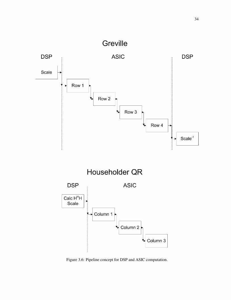
Because in the Greville algorithm, all four rows must be computed, while only three

columns of the Householder decomposition must be computed, there are differing numbers

of row processors and column processors. The high-level pipeline demonstrating the pro-

cessing stages of the Greville and Householder algorithms is shown in Fig. 3.6. The “Scale”

and “Calc HHH and Scale” stages represent the initial processing stages performed on the

DSP, while the “Row n” and “Column n” blocks represent one iteration through the ASIC

in the Greville and Householder implementations respectively.

The first and last stage of the Greville implementation and the first stage in the House-

holder implementation was created by using the DSP baseline code and removing the op-

erations which are calculated on the DSP, as specified in Figs.3.4 and 3.5. Communication

to and from the ASIC was assumed to be via a shared buffer seen as volatile memory to the

DSP, implemented in the DSP chip’s cache. The input matrices were calculated and written

to an input buffer, and the output was immediately read from the output buffer, as shown in

Fig. 3.7. In actual implementation, the read would produce the output from several stages

prior, which can be corrected in code with little cost, shown in Fig. 3.8. The number of

29

cycles spent in this DSP software part of the pipeline was collected for each implemen-

tation by profiling these functions in the CCS profiler and recording the cycle counts in a

modified version of SimpleScalar. Details on the profiler and SimpleScalar are available in

the results section.

3.5.2 ASIC Stages

The PICO Extreme environment provides integrated synthesis and verification tools to

translate unthreaded C-Code into a technology-specific RTL model of an ASIC. The over-

all flow of the PICO software is shown in 3.9. Sequential C-Code is first converted into

C with fixed-length loops. Each loop (and each block of code not within any loop) is re-

written as an individual thread to produce a threaded C implementation. The output from

this threaded model is compared against the original outputs to verify correctness. After

this stage, bit sizes of variables are reduced. If only the first six bits of an eight-bit value are

used, the variable in hardware is reduced to a six-bit variable. This bit-accurate threaded

implementation is again compared against the original for correct output. Next, threaded,

bit-accurate C is translated into a hardware description language and the result is simulated

and compared against the original. Finally, the HDL is synthesized into an RTL package.

The complexity of a single ASIC capable of performing three column stages for the

Householder or four rows for the Greville implementation was too high for PICO to prop-

erly synthesize. In order to reduce complexity, a general processor capable of performing

any ASIC stage of the pipeline was created. This processor would read the input matrix

and data indicating which row or column to process and output accordingly. Three (or

four, for the Greville algorithm) of these processors in a pipeline would produce the cor-

rect output while still remaining synthesizable in PICO. A C-function was written to read

input matrices from a stream (FIFO streams are the preferred method of communication

in PICO – the software automatically determines the ideal width and depth) and take in a

row/column indicator variable as an input. The data flow for a single ASIC processor is

30

shown in Fig. 3.10. A single row/column processor was successfully synthesized for both

implementations.

The PICO software is also capable of creating different RTL implementations based on

differing timing constraints. The user is able to provide a targeted maximum number of

clock cycles taken per stage (Maximum Inter Task Interval – MITI) and the software uses

higher-speed components and achieves higher levels of parallelism by using more compo-

nents in order to achieve this target. To provide a tradeoff between complexity and speedup,

different implementations with different target MITIs were generated. It was noted that as

timing constraints tightened, multipliers were switched from two-cycle to one-cycle and the

number of multipliers increased to be able to complete complex multiplications (requiring

three multiplies) in a single cycle.

31

Figure 3.3: Bit errors for every element of the matrix after two, three, and four iterations of the mainloop in the Greville method.

32

Figure 3.4: Processing locations of Householder block diagram.

33

Figure 3.5: Processing locations of Greville block diagram.

34

Figure 3.6: Pipeline concept for DSP and ASIC computation.

35

Figure 3.7: Communication between DSP and Co-processor via shared buffer.

Figure 3.8: Pipeline showing delay on read for matrix processing.

36

Figure 3.9: General flow for C-Code to RTL in PICO [4].

Figure 3.10: Data flow between DSP and ASICs in FIFOs.

37

Chapter 4

Results

To compare the performance of the baseline DSP-only implementation to the DSP+ASIC

implementation, the number of cycles taken to compute 256 matrices was computed for

each implementation, as 256 is the maximum number of OFDM sub-channels in an IEEE

802.11n client receiver and it is a typical number of sub-channels for other clients in other

protocols. The number of cycles to compute for the ASIC+DSP implementation was com-

puted by assuming that each ASIC processor had fixed, identical latency. In cases where

the DSP pre-processing and shifting stage, shown in Figs. 3.4 and 3.5, took longer than an

ASIC stage, Eq. (4.1) was used. In cases where the ASIC was the longer stage, Eq. (4.2)

was used. In both equations, n is the number of ASIC stages (three for Householder, four

for Greville).

Cycles = 256(cyclesDSP ) + n(cyclesASIC) (4.1)

Cycles = cyclesDSP + (255 + n)cyclesASIC (4.2)

4.1 Determining Baseline Cycles

The Baseline DSP code, included in Appendix A for the Householder implementation and

Appendix B for the Greville implementation, was profiled by using the test wrapper code,

also included in the above appendices. A test file of 1024 test input matrices, modeled

38

after a hypothetical urban pedestrian environment [18], was used as the input for all tests,

included in Appendix C. Code was compiled in CCS with debugging disabled for all files

but the test wrapper. All files but the test wrapper also had file level (-o3) optimization level

enabled.

The number of cycles spent in the test code was determined by using the CCS profiler

and recording the number of cycles spent in the main function under test. To determine the

number of cycles spent in the test functions in the SimpleScalar simulator, the simulator

had to be modified. Additional inputs to the simulator were added to control a counter.

When the simulator program counter reached the first input, the function entry point, a

counter would increase once per simulated clock cycle. Once the second input, the function

exit point, was reached, the counter would stop incrementing. Breakpoints were set at

the function entry and exit points in CCS to determine these memory locations for use in

SimpleScalar. The modified version of SimpleScalar, with additional inputs and counter, is

included in Appendix D. Both the CCS and SimpleScalar results of total cycles were then

divided by the number of input matrices (1024) to determine an average number of cycles

per matrix.

4.2 Determining DSP Pre-process Cycles for Co-processor Implemen-

tations

The number of cycles spent in the pre-process stage was determined in CCS and Sim-

pleScalar using the same method as the baseline. Code for the pre-process, write, and

read operations for each implementation is included in Appendix E for the Householder

implementation and Appendix F for the Greville implementation.

39

4.3 Determining Cycles spent on ASIC for Co-processor Implementa-

tions

To create a PICO generated RTL implementation, code was broken into PICO-friendly

(fixed length loop, stream communicating) row or column processors, included in Ap-

pendix G for the Householder implementation and Appendix H for the Greville implemen-

tation. All other necessary files (also included in the previously mentioned appendices)

were also included in the projects. Implementations were created using both 500 MHz and

1 GHz clocks, with initial specified MITI values of zero. A MITI value of zero causes PICO

to ignore the timing constraint and attempt to produce a low-complexity implementation,

resulting in an output MITI of 332 for the Householder implementation and 235 for the

Greville implementation for both clocks. To produce higher complexity implementations,

these initial maximum MITI values were reduced by ten until synthesis was no longer pos-

sible. Resulting ranges were 230 to 330 for the Householder implementation and 130 to

210 for the Greville implementation. Note that MITI values of 220 and 230 were used for

the Greville implementation, but these resulted in implementations which were had both

higher complexity and higher latency than the 210 MITI implementation, and they were

therefore removed.

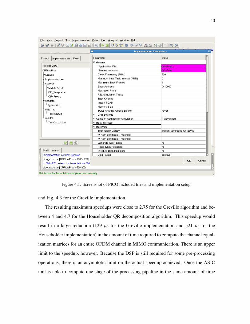
A sample setup of PICO Extreme, with included files (left) and implementation paramters

is shown in Fig. 4.1. All implementations used TSMC 65 target technology files. The maxi-

mum delivered MITI (determined from the PICO command line output from the scheduling

stage) was recorded for each implementation. To translate these numbers into DSP clock

cycles, the 500 MHz implementation MITIs were doubled, as the DSP has a 1 GHz clock.

The resulting speedup was calculated as the ratio of cycles on the DSP only implemen-

tation to the cycles of the DSP and ASIC implementation. The resulting area was calcluated

by using the given estimate of 854,000 gates per mm2. A plot of speedup vs. complexity for

both clocks and both simulators is shown in Fig. 4.2 for the Householder implementation

40

Figure 4.1: Screenshot of PICO included files and implementation setup.

and Fig. 4.3 for the Greville implementation.

The resulting maximum speedups were close to 2.75 for the Greville algorithm and be-

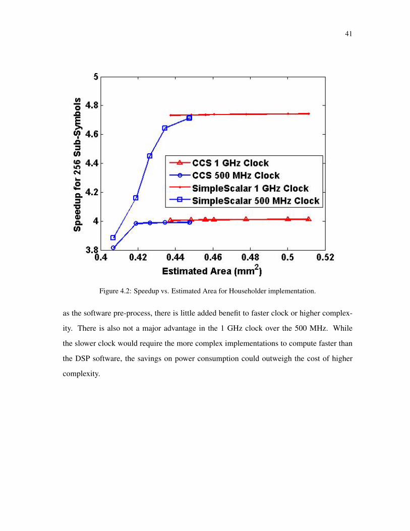
tween 4 and 4.7 for the Householder QR decomposition algorithm. This speedup would

result in a large reduction (129 µs for the Greville implementation and 521 µs for the

Householder implementation) in the amount of time required to compute the channel equal-

ization matrices for an entire OFDM channel in MIMO communication. There is an upper

limit to the speedup, however. Because the DSP is still required for some pre-processing

operations, there is an asymptotic limit on the actual speedup achieved. Once the ASIC

unit is able to compute one stage of the processing pipeline in the same amount of time

41

Figure 4.2: Speedup vs. Estimated Area for Householder implementation.

as the software pre-process, there is little added benefit to faster clock or higher complex-

ity. There is also not a major advantage in the 1 GHz clock over the 500 MHz. While

the slower clock would require the more complex implementations to compute faster than

the DSP software, the savings on power consumption could outweigh the cost of higher

complexity.

42

Figure 4.3: Speedup vs. Estimated Area for Greville implementation.

43

Chapter 5

Conclusions and Future Work

To support the operations required by MIMO wireless communication, two different meth-

ods of enhancing current DSPs were investigated. Additional instructions on the DSP did

result in an improvement, but it was not sufficient to allow current technology to support

current MIMO wireless protocols. Two hardware co-processors were designed, one for

a Householder decomposition algorithm and one for a Greville pseudo inverse algorithm.

These hardware co-processors resulted in a simulated speedup of 2.7 for the Greville algo-

rithm and between 4 and 4.7 for the Householder algorithm.

In practice, a hardware co-processor capable of performing various matrix operations

would be preferable to the ASIC units designed in this work. A programmable processor

would not be algorithm dependent and therefore one processor would be applicable to

both algorithms used in this work, as well as many other possible algorithms. This is a

similar approach to current hardware trends, where on-board programmable processors can

quickly compute audio and video encoding or various encryption techniques. Future work

would include design of a programmable hardware co-processor capable of performing

many general matrix operations required by various equalization matrix algorithms.

44

Bibliography

[1] PICO RTL: Synthesis, Verification and Integration Guide. Oct. 2008.

[2] IEEE Standard for Information technology–Telecommunications and information ex-change between systems–Local and metropolitan area networks–Specific require-ments Part 11: Wireless LAN Medium Access Control (MAC) and Physical Layer(PHY) Specifications Amendment 5: Enhancements for Higher Throughput. IEEEStd 802.11n-2009 (Amendment to IEEE Std 802.11-2007 as amended by IEEEStd 802.11k-2008, IEEE Std 802.11r-2008, IEEE Std 802.11y-2008, and IEEE Std802.11w-2009), pages c1–502, 29 2009.

[3] Overview of 3GPP Release 8 V0.0.8. Aug. 2009.

[4] TMS320C64x/C64x+ DSP CPU and Instruction Set. Aug. 2009.

[5] TMS320DM6467T Digital Media System-on-Chip. Nov. 2009.

[6] 3rd Generation Partnership Project. Technical Specification Group Radio Access Net-work: Physical layer aspects for evolved Universal Terrestrial Radio Access (UTRA)(Release 7), 2006.

[7] IEEE 802.16. Air Interface for Fixed and Mobile Broadband Wireless Access Sys-tems, Feb. 2006.

[8] C.A. Belfiore and Jr. Park, J.H. Decision Feedback Equalization. Proceedings of theIEEE, 67(8):1143–1156, Aug. 1979.

[9] Kuo-Liang Chung and Wen-Ming Yan. The Complex Householder Transform. SignalProcessing, IEEE Transactions on, 45(9):2374–2376, Sep 1997.

[10] Jr. Cimini, L. Analysis and Simulation of a Digital Mobile Channel Using Orthog-onal Frequency Division Multiplexing. Communications, IEEE Transactions on,33(7):665–675, Jul 1985.

[11] Peter C. Cramton. Money Out of Thin Air: The Nationwide Narrowband PCS Auc-tion. Journal of Economics and Management Strategy, 4:267–343, 1995.

45

[12] Bier J. Eyre, J. DSP Processors Hit the Mainstream. Computer, 31(8):51 –59, Aug1998.

[13] D. Gesbert, M. Shafi, Da shan Shiu, P.J. Smith, and A. Naguib. From Theory toPractice: an Overview of MIMO Space-Time Coded Wireless Systems. SelectedAreas in Communications, IEEE Journal on, 21(3):281–302, Apr 2003.

[14] Gene H. Golub and Charles F. Van Loan. Matrix Computations. The Johns HopkinsUniversity Press, Baltimore, MD, 3 edition, 1996.

[15] K. Ho and A. Kwasinski. Uplink Channel Estimation in WiMAX. In Wireless Com-munications and Networking Conference, 2009. WCNC 2009. IEEE, pages 1–6, April2009.

[16] Ibing A. Kuhling, D. A Novel Low-Complexity Algorithm for Linear MMSE MIMOReceivers. pages 401 –405, May 2008.

[17] E.G. Larsson. MIMO Detection Methods: How They Work [Lecture Notes]. SignalProcessing Magazine, IEEE, 26(3):91–95, May 2009.

[18] K. J. Ray Liu, A. K. Sadek, W. Su, and A. Kwasinski. Cooperative Communicationsand Networking. Cambridge University Press, New York, NY, USA, 2009.

[19] Thomas L. Marzetta. BLAST Training: Estimating Channel Characteristics for HighCapacity Space-Time Wireless. In Proc. 37th Annual Allerton Conference on Com-munications, Control, and Computing, pages 958–966, 1999.

[20] S.A. Mujtaba. MIMO Signal Processing - the Next Frontier for Capacity Enhance-ment. In Custom Integrated Circuits Conference, 2003. Proceedings of the IEEE2003, pages 263–270, Sept. 2003.

[21] Chitranjan K. Singh, Sushma H. Prasad, and Poras T. Balsara. A Fixed-Point Imple-mentation for QR Decomposition. In Design, Applications, Integration and Software,2006 IEEE Dallas/CAS Workshop on, pages 75–78, Oct. 2006.

[22] Qinfang Sun, D.C. Cox, H.C. Huang, and A. Lozano. Estimation of ContinuousFlat Fading MIMO Channels. Wireless Communications, IEEE Transactions on,1(4):549–553, Oct 2002.

[23] J.J. van de Beek, M. Sandell, and P.O. Borjesson. ML estimation of time andfrequency offset in OFDM systems. Signal Processing, IEEE Transactions on,45(7):1800–1805, Jul 1997.

46

[24] E. Viterbo and J. Boutros. A Universal Lattice Code Decoder for Fading Channels.Information Theory, IEEE Transactions on, 45(5):1639–1642, Jul 1999.

[25] P.W. Wolniansky, G.J. Foschini, G.D. Golden, and R.A. Valenzuela. V-BLAST: anArchitecture for Realizing Very High Data Rates Over the Rich-Scattering WirelessChannel. In Proceedings of URSI International Symposium on Signals, Systems, andElectronics, 1998., pages 295–300, Sep-2 Oct 1998.

47

Appendix A

Base DSP Householder Implementation Codeand Test Wrapper

Included on disk.

48

Appendix B

Base DSP Greville Implementation Code andFile Test Wrapper

Included on disk.

49

Appendix C

Test Matrices

Included on disk.

50

Appendix D

Modified SimpleScalar Code

Included on disk.

51

Appendix E

DSP and Co-processor Householder DSP Code

Included on disk.

52

Appendix F

DSP and Co-processor Greville DSP Code

Included on disk.

53

Appendix G

DSP and Co-processor Householder ASIC Col-umn Processor Code

Included on disk.

54

Appendix H

DSP and Co-processor Greville ASIC Row Pro-cessor Code

Included on disk.