hardness of approximating the minimum distance of a ...cseweb.ucsd.edu/~daniele/papers/dms.pdfour...
TRANSCRIPT

Hardness of Approximating the Minimum Distance of a Linear
Code∗
Ilya Dumer† Daniele Micciancio ‡ Madhu Sudan§
April 15, 2007
Abstract
We show that the minimum distance d of a linear code is not approximable to within anyconstant factor in random polynomial time (RP), unless NP (nondeterministic polynomial time)equals RP. We also show that the minimum distance is not approximable to within an additiveerror that is linear in the block length n of the code. Under the stronger assumption that NPis not contained in RQP (random quasi-polynomial time), we show that the minimum distance
is not approximable to within the factor 2log1−ǫ(n), for any ǫ > 0. Our results hold for codesover any finite field, including binary codes. In the process we show that it is hard to findapproximately nearest codewords even if the number of errors exceeds the unique decodingradius d/2 by only an arbitrarily small fraction ǫd. We also prove the hardness of the nearestcodeword problem for asymptotically good codes, provided the number of errors exceeds (2/3)d.
Our results for the minimum distance problem strengthen (though using stronger assump-tions) a previous result of Vardy who showed that the minimum distance cannot be computedexactly in deterministic polynomial time (P), unless P = NP. Our results are obtained byadapting proofs of analogous results for integer lattices due to Ajtai and Micciancio. A criticalcomponent in the adaptation is our use of linear codes that perform better than random (linear)codes.
1 Introduction
In this paper we study the computational complexity of two central problems from coding theory:(1) The complexity of approximating the minimum distance of a linear code and (2) The complexityof error-correction in codes of relatively large minimum distance. An error-correcting code A ofblock length n over a q-ary alphabet Σ is a collection of strings (vectors) from Σn, called codewords.For all codes considered in this paper, the alphabet size q is always a prime power and the alphabetΣ = Fq is the finite field with q element. A code A ⊆ F
nq is linear if it is closed under addition and
∗An edited version of this paper appears in IEEE Transactions on Information Theory, 49(1):22-37, January 2003.This is the authors’ copy.
†College of Engineering, University of California at Riverside. Riverside, CA 92521, USA. Email:[email protected]. Research supported in part by NSF grant NCR-9703844.
‡Department of Computer Science and Engineering, University of California at San Diego. La Jolla, CA 92093-0114, USA. Email: [email protected]. Research supported in part by NSF Career Award CCR-0093029.
§Department of Electrical Engineering and Computer Science, Massachusetts Institute of Technology. 545 Technol-ogy Square, Cambridge, MA 02139, USA. Email: [email protected]. Research supported in part by a Sloan FoundationFellowship, an MIT-NEC Research Initiation Grant and NSF Career Award CCR-9875511.

multiplication by a scalar, i.e., A is a linear subspace of Fnq over base field Fq. For such a code, the
information content (i.e., the number k = logq |A| of information symbols that can be encoded witha codeword1) is just its dimension as a vector space and the code can be compactly representedby a k × n generator matrix A ∈ F
k×nq of rank k such that A = {xA | x ∈ F
kq}. An important
property of a code is its minimum distance. For any vectors x,y ∈ Σn, the Hamming weight ofx is the number wt(x) of nonzero coordinates of x. The weight function wt(·) is a norm, and theinduced metric d(x,y) = wt(x−y) is called the Hamming distance. The (minimum) distance d(A)of the code A is the minimum Hamming distance d(x,y) taken over all pairs of distinct codewordsx,y ∈ A. For linear codes it is easy to see that the minimum distance d(A) equals the weightwt(x) of the lightest nonzero codeword x ∈ A \ {0}. If A is a linear code over Fq with blocklength n, rank k and minimum distance d, then it is customary to say that A is a linear [n, k, d]qcode. Throughout the paper we use the following notational conventions: matrices are denotedby boldface uppercase Roman letters (e.g., A,C), the associated linear codes are denoted by thecorresponding calligraphic letters (e.g., A, C), and we write A[n, k, d]q to mean that A is a linearcode over Fq with block length n, information content k and minimum distance d.
1.1 The Minimum Distance Problem
Three of the four central parameters associated with a linear code, namely n, k and q, are evidentfrom its matrix representation. The minimum distance problem (MinDist) is that of evaluatingthe fourth — namely — given a generator matrix A ∈ F
k×nq find the minimum distance d of the
corresponding code A. The minimum distance of a code is obviously related to its error correctioncapability ⌊(d − 1)/2⌋ and therefore finding d is a fundamental computational problem in codingtheory. The problem gains even more significance in light of the fact that long q-ary codes chosenat random give the best parameters known for any q < 46 (in particular, for q = 2)2. A polynomialtime algorithm to compute the distance would be the ideal solution to the problem, as it couldbe used to construct good error correcting codes by choosing a generator matrix at random andchecking if the associated code has a large minimum distance. Unfortunately, no such algorithmis known. The complexity of this problem (can it be solved in polynomial time or not?) wasfirst explicitly questioned by Berlekamp, McEliece and van Tilborg [5] in 1978 who conjectured itto be NP-complete. This conjecture was finally resolved in the affirmative by Vardy [23, 22] in1997, proving that the minimum distance cannot be computed in polynomial time unless P = NP.([23, 22] also give further motivations and detailed account of prior work on this problem.)
To advance the search of good codes, one can relax the requirement of computing d exactly intwo ways:
• Instead of requiring the exact value of d, one can allow for approximate solutions, i.e., anestimate d′ that is guaranteed to be at least as big, but not much bigger than the trueminimum distance d. (E.g., d ≤ d′ ≤ γd for some approximation factor γ).
• Instead of insisting on deterministic solutions that always produce correct (approximate) an-swers, one can consider randomized algorithms such that d′ ≤ γd only holds in a probabilistic
1Throughout the paper, we write log for the logarithm to the base 2, and logq when the base q is any numberpossibly different from 2.
2For square prime powers q ≥ 49, linear AG codes can perform better than random ones [21] and are constructiblein polynomial time. For all other q ≥ 46 it is still possible to do better than random codes, however the best knownprocedures to construct them run in exponential time [24].
2
sense. (Say d′ ≤ γd with probability at least 1/2.)3
Such algorithms can still be used to randomly generate relatively good codes as follows. Say wewant a code with minimum distance d. We pick a generator matrix at random such that the codeis expected to have minimum distance γd. Then, we run the probabilistic distance approximationalgorithm many times using independent coin tosses. If all estimates returned by the distanceapproximation algorithm are at least γd, then the minimum distance of the code is at least d withvery high probability.
In this paper, we study these more relaxed versions of the minimum distance problem and showthat the minimum distance is hard to approximate (even in a probabilistic sense) to within anyconstant factor, unless NP = RP (i.e., every problem in NP has a polynomial time probabilisticalgorithm that always rejects No instances and accepts Yes instances with high probability). Underthe stronger assumption that NP does not have random quasi-polynomial4 time algorithms (RQP),we prove that the minimum distance of a code of block length n is not approximable to within
a factor of 2log(1−ǫ) n for any constant ǫ > 0. (This is a naturally occurring factor in the studyof the approximability of optimization problems — see the survey of Arora and Lund [4].) Ourmethods adapt the proof of the inapproximability of the shortest lattice vector problem (SVP) dueto Micciancio [18] (see also [19]) which in turn is based on Ajtai’s proof of the hardness of solvingSVP [2].
1.2 The Error Correction Problem
In the process of obtaining the inapproximability result for the minimum distance problem, we alsoshed light on the general error-correction problem for linear codes. The simplest formulation is theNearest Codeword Problem (NCP) (also known as the “maximum likelihood decoding problem”).Here, the input instance consists of a generator matrix A ∈ F
k×nq and a received word x ∈ F
nq
and the goal is to find the nearest codeword y ∈ A to x. A more relaxed version is to estimatethe minimum “error weight” d(x,A) that is the distance d(x,y) to the nearest codeword, withoutnecessarily finding codeword y. The NCP is a well-studied problem: Berlekamp, McEliece and vanTilborg [5] showed that it is NP-hard (even in its weight estimation version); and more recentlyArora, Babai, Stern and Sweedyk [3] showed that the error weight is hard to approximate to
within any constant factor unless P = NP, and within factor 2log(1−ǫ) n for any ǫ > 0, unlessNP ⊆ QP (deterministic quasi-polynomial time). This latter result has been recently improved toinapproximability within 2O(log n/ log log n) = n1/O(log log n) under the assumption that P 6= NP byDinur, Kindler, Raz and Safra [9, 8]). On the positive side, NCP can be trivially approximatedwithin a factor n. General, non-trivial approximation algorithms have been recently discovered byBerman and Karpinski [6], who showed that (for any finite field Fq) NCP can be approximatedwithin a factor ǫn/ log n for any fixed ǫ > 0 in probabilistic polynomial time, and ǫn in deterministicpolynomial time.
However the NCP only provides a first cut at understanding the error-correction problem. Itshows that the error-correction problem is hard, if we try to decode every linear code regardlessof the error weight. In contrast, the positive results from coding theory show how to performerror-correction in specific linear codes corrupted by errors of small weight (relative to the code
3One can also consider randomized algorithms with 2-sided error, where also the lower bound d′ ≥ d holds onlyin a probabilistic sense. All our results can be easily adapted to algorithms with 2-sided error.
4f(n) is quasi-polynomial in n if it grows slower than 2logc n for some constant c.
3

distance). Thus the hardness of the NCP may come from one of two factors: (1) The problemattempts to decode every linear code and (2) The problem attempts to recover from too manyerrors. Both issues have been raised in the literature [23, 22], but only the former has seen someprogress [7, 10, 20].
One problem that has been defined to study the latter phenomenon is the “Bounded distancedecoding problem” (BDD, see [23, 22]). This is a special case of the NCP where the error weight isguaranteed (or “promised”) to be less than d(A)/2. This case is motivated by the fact that withinsuch a distance, there may be at most one codeword and hence decoding is clearly unambiguous.Also this is the case where many of the classical error-correction algorithms (for say BCH codes,RS codes, AG codes, etc.) work in polynomial time.
1.3 Relatively Near Codeword Problem
To compare the general NCP, and the more specific BDD problem, we introduce a parameterizedfamily of problems that we call the Relatively Near Codeword Problem (RNC). For real ρ, RNC
(ρ)
is the following problem:
Given a generator matrix A ∈ Fk×nq of a linear code A of (not necessarily known)
minimum distance d, an integer t with the promise that t < ρ · d, and a received wordx ∈ F
nq , find a codeword within distance t from x. (The algorithm may fail if the
promise is violated, or if no such codeword exists. In other words, in contrast to thepapers [3] and [5], the algorithm is expected to work only when the error weight islimited in proportion to the code distance.)
Both the nearest codeword problem (NCP) and the bounded distance decoding problem (BDD)
are special cases of RNC(ρ): NCP = RNC
(∞) while BDD = RNC( 12). Till recently, not much was
known about RNC(ρ) for constants ρ < ∞, leave alone ρ = 1
2 (i.e., the BDD problem). No finiteupper bound on ρ can be easily derived from Arora et al.’s NP-hardness proof for NCP [3]. (Inother words, their proof does not seem to hold for RNC
(ρ) for any ρ < ∞.) It turns out, as observedby Jain et al. [14], that Vardy’s proof of the NP-hardness of the minimum distance problem alsoshows the NP-hardness of RNC
(ρ) for ρ = 1 (and actually extends to some ρ = 1 − o(1)).In this paper we significantly improve upon this situation, by showing NP-hardness (under ran-
domized reductions) of RNC(ρ) for every ρ > 1
2 bringing us much closer to an eventual (negative?)resolution of the bounded distance decoding problem.
1.4 Organization
The rest of the paper is organized as follows. In Section 2 we precisely define the coding prob-lems studied in this paper, introduce some notation, and briefly overview the random reductiontechniques and coding theory notions used in the rest of the paper. As explained in Section 2 ourproofs rely on coding theoretic constructions that might be of independent interest, namely theconstruction of codes containing unusually dense clusters. These constructions constitute the maintechnical contribution of the paper, and are presented in Section 3 (for arbitrary linear codes) andSection 6 (for asymptotically good codes). The hardness of the relatively near codeword problemand the minimum distance problem are proved in Sections 4 and 5 respectively. Similar hardnessresults for asymptotically good codes are presented in Section 7. The reader mostly interested in
4

computational complexity may want to skip Section 3 at first reading, and jump directly to theNP-hardness results in Sections 4 and 5. Section 8 concludes with a discussion of the consequencesand limitations of the proofs given in this paper, and related open problems.
2 Background
2.1 Approximation Problems
In order to study the computational complexity of coding problems, we formulate them in terms ofpromise problems. A promise problem is a generalization of the familiar notion of decision problem.The difference is that in a promise problem not every string is required to be either a Yes or a No
instance. Given a string with the promise that it is either a Yes or No instance, one has to decidewhich of the two sets it belongs to.
The following promise problem captures the hardness of approximating the minimum distanceproblem within a factor γ.
Definition 1 (Minimum Distance Problem) For prime power q and approximation factor γ ≥1, an instance of GapDistγ,q is a pair (A, d), where A ∈ F
k×nq and d ∈ Z
+, such that
• (A, d) is a Yes instance if d(A) ≤ d.
• (A, d) is a No instance if d(A) > γ · d.
In other words, given a code A and an integer d with the promise that either d(A) ≤ d ord(A) > γ ·d, one must decide which of the two cases holds true. The relation between approximatingthe minimum distance of A and the above promise problem is easily explained. On the one hand,if one can compute a γ-approximation d′ ∈ [d(A), γ · d(A)] to the minimum distance of the code,then one can easily solve the promise problem above by checking whether d′ ≤ γ ·d or d′ > γ ·d. Onthe other hand, assume one has a decision oracle O that solves the promise problem above. Then,the minimum distance of a given code A can be easily approximated using the oracle as follows.Notice that O(A, n) always returns Yeswhile O(A, 0) always returns No. Using binary search,one can efficiently find a number d such that O(A, d) = Yes and O(A, d − 1) = No.5 This meansthat (A, d) is not a No instance and (A, d − 1) is not a Yes instance, and the minimum distanced(A) must lie in the interval [d, γ · d].
Similarly we can define the following promise problem to capture the hardness of approximatingRNC
(ρ) within a factor γ.
Definition 2 (Relatively Near Codeword Problem) For prime power q, and factors ρ > 0
and γ ≥ 1, an instance of GapRNC(ρ)γ,q is a triple (A,v, t), where A ∈ F
k×nq , v ∈ F
nq and t ∈ Z
+,such that t < ρ · d(A) and 6
• (A,v, t) is a Yes instance if d(v,A) ≤ t.
• (A,v, t) is a No instance if d(v,A) > γt.
5By definition, the oracle can give any answer if the input is neither a Yes instance nor a No one. So, it wouldbe wrong to conclude that (A, d − 1) is a No instance and (A, d) is a Yes one.
6Strictly speaking, the condition t < ρ · d(CA) is a promise and hence should be added as a condition in both theYes and No instances of the problem.
5
It is immediate that the problem RNC(ρ) gets harder as ρ increases, since changing ρ has the
only effect of weakening the promise t < ρ · d(A). RNC(ρ) is the hardest when ρ = ∞ in which
case the promise t < ρd(A) is vacuously true and we obtain the familiar (promise version of) thenearest codeword problem:
Definition 3 (Nearest Codeword Problem) For prime power q and γ ≥ 1, an instance ofGapNCPγ,q is a triple (A,v, t), A ∈ F
k×nq , v ∈ F
nq and t ∈ Z
+, such that
• (A,v, t) is a Yes instance if d(v,A) ≤ t.
• (A,v, t) is a No instance if d(v,A) > γ · t.
The promise problem GapNCPγ,q is NP-hard for every constant γ ≥ 1 (cf. [3]7), and this resultis critical to our hardness result(s). We define one last promise problem to study the hardness ofapproximating the minimum distance of a code with linear additive error.
Definition 4 For τ > 0 and prime power q, let GapDistAddτ,q be the promise problem withinstances (A, d), where A ∈ F
k×nq and d ∈ Z
+, such that
• (A, d) is a Yes instance if d(A) ≤ d
• (A, d) is a No instance if d(A) > d + τ · n.
2.2 Random Reductions and Techniques
The main result of this paper (see Theorem 22) is that approximation problem GapDistγ,q isNP-hard for any constant factor γ ≥ 1 under polynomial reverse unfaithful random reductions
(RUR-reductions, [15]), and for γ = 2log(1−ǫ) n = n1/ logǫ(n) it is hard under quasi-polynomial RUR-reductions. These are probabilistic reductions that map No instances always to No instances andYes instances to Yes instances with high probability. In particular, given a security parameters, all reductions presented in this paper warrant that Yes instances are properly mapped withprobability 1 − q−s in poly(s) time.8 The existence of a (random) polynomial time algorithm tosolve the hard problem would imply NP = RP (random polynomial time), i.e., every problem in NPwould have a probabilistic polynomial time algorithm that always rejects No instances and acceptsYes instances with high probability.9 Similarly, hardness for NP under quasi-polynomial RUR-reductions implies that the hard problem cannot be solved in RQP unless NP ⊆ RQP (random
7To be precise, Arora et al. [3] present the result only for binary codes. However, their proof is valid for anyalphabet. An alternate way to obtain the result for any prime power is to use a recent result of Hastad [13] whostates his result in linear algebra (rather than coding-theoretic) terms. We will state and use some of the additionalfeatures of the latter result in Section 7.
8Here, and in the rest of the paper, we use notation poly(n) to denote any polynomially bounded function of n,i.e., any function f(n) such that f(n) = O(nc) for some constant c indepentent of n.
9Notice that we are unable to prove that the existence of a polynomial time approximation algorithm implies thestronger containment NP ⊆ ZPP (ZPP is the class of decision problems L such that both L and its complement are inRP, i.e., ZPP = RP∩ coRP), as done for example in [12]. The difference is that [12] proves hardness under unfaithful
random reductions (UR-reductions [15], i.e. reductions that are always correct on Yes instances and often correct onNo instances). Hardness under UR-reductions implies that no polynomial time algorithm exists unless NP ⊆ coRP,and therefore RP ⊆ NP ⊆ coRP. It immediately follows that coRP ⊆ RP and NP = RP = coRP = ZPP. However,in our case where RUR-reductions are used, we can only conclude that RP ⊆ NP ⊆ RP, and therefore NP = RP, butit is not clear how to establish any relation involving the complementary class coRP and ZPP.
6

quasi-polynomial time). Therefore, similarly to a proper NP-hardness result (obtained under de-terministic polynomial reductions), hardness under polynomial RUR-reductions also gives evidenceof the intractability of a problem.
In order to prove these results, we first study the problem GapRNC(ρ)γ,q. We show that the
error weight is hard to approximate to within any constant factor γ and for any ρ > 1/2 unlessNP = RP (see Theorem 16). By using γ = 1/ρ, we immediately reduce our error-correction problem
GapRNC(ρ)γ,q to the minimum distance problem GapDistγ,q for any constant γ < 2. We then use
product constructions to “amplify” the constant and prove the claimed hardness results for theminimum distance problem.
The hardness of GapRNC(ρ)γ,q for ρ > 1/2 is obtained by adapting a technique of Micciancio [18],
which is in turn based on the work of Ajtai [2] (henceforth Ajtai-Micciancio). They consider theanalogous problem over the integers (rather than finite fields) with Hamming distance replaced byEuclidean distance. Much of the adaptation is straightforward; in fact, some of the proofs are eveneasier in our case due to the use of finite fields. The main hurdle turns out to be in adapting thefollowing combinatorial problem considered and solved by Ajtai-Micciancio:
Given an integer k construct, in poly(k) time, integers r, l, an l-dimensional latticeL (i.e., a subset of Z
l closed under addition and multiplication by an integer) withminimum (Euclidean) distance d > r/ρ and a vector v ∈ Z
l such that the (Euclidean)ball of radius r around v contains at least 2k vectors from L (where ρ < 1 is a constantindependent of k).
In our case we are faced with a similar problem with Zl replaced by F
lq and Euclidean dis-
tance replaced by Hamming distance. The Ajtai-Micciancio solution to the above problem involvesnumber-theoretic methods and does not translate to our setting. Instead we show that if we con-sider a linear code whose performance (i.e., trade-off between rate and distance) is better than thatof a random code, and pick a random light vector in F
nq , then the resulting construction has the
required properties. We first solve this problem over sufficiently large alphabets using high rateReed-Solomon (RS) codes. (See next subsection for the definition RS codes. This same constructionhas been used in the coding theory literature to demonstrate limitations to the “list-decodability”of RS codes [16].) We then translate the result to small alphabets using the well-known method ofconcatenating codes [11].
In the second part of the paper, we extend our methods to address asymptotically-good codes.We show that even for such codes, the Relatively Near Codeword problem is hard unless NP equals
RP (see Theorem 31), though for these codes we are only able to prove the hardness of GapRNC(ρ)γ,q
for ρ > 2/3. Finally, we translate this to a result (see Theorem 32) showing that the minimumdistance of a code is hard to approximate to within an additive error that is linear in the blocklength of the code.
2.3 Coding Theory
For a through introduction to coding theory the reader is referred to [17]. Here we briefly reviewsome basic results as used in the rest of the paper. Readers with an adequate background in codingtheory can safely skip to the next section.
A classical problem in coding theory is to determine for given alphabet Fq, block length n anddimension k, what is the highest possible minimum distance d such that there exists a [l,m, d]q
7

linear code. The following two theorems give well known upper and lower bounds for d.
Theorem 5 (Gilbert-Varshamov bound) For finite field Fq, block length l and dimension m ≤l, there exists a linear code A[l,m, d]q with minimum distance d satisfying
qm−l · |B(0, d − 1)| ≥ 1 (1)
where |B(0, d − 1)| =∑d−1
r=0
( lr
)(q − 1)r is the volume of the l dimensional Hamming sphere of
radius d − 1. For any m ≤ l, the smallest d such that (1) holds true is denoted d∗m. (Notice thatthe definition of d∗m depends both on the information content m and the block length l. For brevity,we omit l from the notation, as the block length is usually clear from the context.)
See [17] for a proof. The upper bound on d given by the Gilbert-Varshamov theorem (GVbound, for short) is not effective, i.e., even if the theorem guarantees the existence of linear codeswith a certain minimum distance, the proof of the theorem employs a greedy algorithm that runsin exponential time, and we do not know any efficient way to find such codes for small alphabetsq < 49. Interestingly, random linear codes meet the GV bound, i.e., if the generating matrix ofthe code is chosen uniformly at random, then the minimum distance of the resulting code satisfiesthe GV bound with high probability. However, given a randomly chosen generator matrix, it is notclear how to efficiently check whether the corresponding code meets the GV bound or not. We nowgive a lower bound on d.
Theorem 6 (Singleton bound) For every linear code C[l,m, d]q, the minimum distance d is atmost
d ≤ l − m + 1.
See [17] for a proof. A code C[l,m, d]q is called Maximum Distance Separable (MDS) if theSingleton bound is satisfied with equality, i.e., if d = l−m+1. Reed-Solomon codes are an importantexample of MDS codes. For any finite field Fq, and dimension m ≤ q−1, the Reed-Solomon code (RScode) G[q−1,m, q−m]q can be defined as the set of (q−1)-dimensional vectors obtained evaluatingall qm polynomials p(x) = c0+c1x+· · · cm−1x
m−1 ∈ Fq[x] of degree less than m at all nonzero pointsx ∈ Fq \{0}. Extended Reed-Solomon codes G[q,m, q−m+1]q are defined similarly, but evaluatingthe polynomials at all points x ∈ Fq, including 0. Since a nonzero polynomial p of degree (m − 1)can have at most (m−1) zeros, then every nonzero (extended) RS codeword has at most m−1 zeropositions, so it’s Hamming weight is at least q −m (resp. q −m + 1). This proves that (extended)Reed-Solomon codes are maximum distance separable. Extended RS codes can be further extendedconsidering the homogeneous polynomials p(x, y) =
∑m−1i=1 aix
iym−1−i, and evaluating them at allpoints of the projective line {(x, 1): x ∈ Fq} ∪ {(1, 0)}. This increases both the block length andthe minimum distance by one, giving twice extended RS codes G[q + 1,m, q − m + 2]q.
Another family of codes we are going to use are the Hadamard codes H[qc − 1, c, qc − qc−1]q.In these codes, each codeword corresponds to a vector x ∈ F
cq. The codeword associated to x is
obtained by evaluating all nonzero linear functions φ : Fcq → Fq at x. Since there are qc linear
functions in c variables (including the zero function), the code has block length qc − 1. Noticethat any nonzero vector x ∈ F
cq is mapped to 0 by exactly a 1/q fraction of the linear functions
φ : Fcq → Fq (including the identically zero function). So the minimum distance of the code is
qc − qc−1.
8

In Section 6 we will also use Algebraic Geometric codes (AG codes). The definition of thesecodes is beyond the scope of the present paper, and the interested reader is referred to [21].
An important operation used to combine codes is the concatenating code construction of [11].Let A and B be two linear codes over alphabets Fqk and Fq, with generating matrices A ∈ F
m×lqk
and B ∈ Fn×kq . A is called the outer code, and B is called the inner code. Notice that the dimension
of the inner code equals the dimension of the alphabet of the outer code Fqk , viewed as a vectorspace over base field Fq. The idea is to replace every component xi of outer codeword [x1, . . . , xl] ∈A ⊆ F
lqk with a corresponding inner codeword φ(xi) ∈ B. More precisely, let α1, . . . , αk ∈ Fqk be
a basis for Fqk as a vector space over Fq and let φ : Fqk → B be the (unique) linear function such
that φ(αi) = bi for all i = 1, . . . , k. The concatenation function 3B : Flqk → F
lnq is given by
[x1, . . . , xn]3B = [φ(x1), . . . , φ(xn)].
Function 3B is extended to sets of vectors in the usual way X3B = {x3B : x ∈ X}, and con-catenated code A3B is just the result of applying the concatenation function 3B to set A. It iseasy to see that if A is a [l,m, d]qk code and B is a [n, k, t]q code, then the concatenation A3B is
a [nl, km, dt]q code with generator matrix C ∈ Fnl×kmq given by
ci+jk = (αi · aj+1)3B.
for all i = 1, . . . , k and j = 0, . . . ,m − 1.
3 Dense Codes
In this section we present some general results about codes with a special density property (to bedefined), and their algorithmic construction. The section culminates with the proof of Lemma 15which shows how to efficiently construct a gadget that will be used in Section 4 in our NP-hardnessproofs. Lemma 15 is in fact the only result from this section directly used in the rest of the paper(with the exception of Section 6 which extends the results of this section to asymptotically goodcodes). The reader mostly interested in computational complexity issues, may want to skip thissection at first reading, and refer to Lemma 15 when used in the proofs.
3.1 General overview
Let B(v, r) = {x ∈ Flq|d(v,x) ≤ r} be the ball of radius r centered in v ∈ F
lq. In this section, we
wish to find codes C[l,m, d]q that include multiple codewords in some ball(s) B(v, r) of relativelysmall radius r = ⌊ρd⌋, where ρ is some positive real number. Obviously, the problem is meaningfulonly for ρ ≥ 1/2, as any ball of radius r < d/2 cannot contain more than a single codeword. Belowwe prove that for any ρ > 1/2 it is actually possible to build such a code. These codes are used in
the sequel to prove the hardness of GapRNC(ρ)γ,q by reduction from the nearest codeword problem.
Of particular interest is the case r < d (i.e., ρ < 1), as the corresponding hardness result forGapRNC can be translated into an inapproximability result for the minimum distance problem.
We say that a code C[l,m, d]q is (ρ, k)-dense around v ∈ Flq if the ball B(v, ⌊ρd⌋) contains at
least qk codewords. We say that C is (ρ, k)-dense if it is (ρ, k)-dense around v for some v. Wewant to determine for what values of the parameters ρ, k, l,m, d there exist (ρ, k)-dense codes. Thetechnique we use is probabilistic: we show that there exist [l,m, d]q codes such that the expected
9

number of codewords in a randomly chosen sphere B(v, ρd) is at least qk. It easily follows, by asimple averaging argument, that there exists a center v such that the code is (ρ, k)-dense aroundv. Let
µC(r) = Expv∈Fl
q
[|C ∩ B(v, r)|] =∑
x∈CPr
v∈Flq
{x ∈ B(v, r)}
be the expected number of codewords in B(v, r) when the center v is chosen uniformly at randomfrom F
lq. Notice that
µC(r) =∑
x∈CPr
v∈Flq
{v ∈ B(x, r)} =|C| · |B(0, r)|
ql= qm−l · |B(0, r)|. (2)
This shows that the average number of codewords in a randomly chosen ball does not depend onthe specific code C, but only on its information content m (and the block length l, which is usuallyimplicit and clear from the context). So, we can simply write µm instead of µC .
In the rest of this subsection, we show how dense codes are closely related to codes that out-perform the GV bound. This connection is not explicitly used in the rest of the paper, and it ispresented here only for the purpose of illustrating the intuition behind the choice of codes used inthe sequel. Using function µm, the definition of the minimum distance (for codes with informationcontent m) guaranteed by the GV bound (see Theorem 5) can be rewritten as
d∗m = min{r | µm(r − 1) ≥ 1}.
In particular, for any code C[l,m, d]q , the expected number of codewords in a random sphere ofradius d∗m is bigger than 1, and there must exist spheres with multiple codewords. If the distanceof the code d exceeds the GV bound for codes with the same information content (i.e., d > d∗m), Cis (ρ, k)-dense for some ρ = d∗m/d < 1 and k > 0. Several codes are known for which the minimumdistance exceeds the GV bound:
• RS codes or, more generally, MDS codes, whose distances d exceed d∗m for all code rates. RScodes of rate m/l approaching 1 will be of particular interest. This is due to the fact that theratio d/d∗m grows with code rate m/l of RS codes and tends to 2 for high rates. We implicitlyuse this fact in the sequel to build a ρ-dense codes for any ρ > 1/2.
• Binary BCH codes, whose distances exceed d∗m for very high code rates approaching 1. Thesecodes are not used in this paper, but they are an important family of codes that beat the GVbound.
• AG codes, meeting the TVZ bound, whose distances exceed d∗m for most code rates boundedaway from 0 and 1 for any q. These codes are used to prove hardness results for asymptoticallygood codes, and approximating the minimum distance up to an additive error.
Remark 7 The relation between dense codes and codes that exceed the GV bound can be given anexact, quantitative characterization. In particular, one can prove that for any positive integer kand real ρ, the expected number of codewords from C[l,m, d] in a random sphere of radius r = ⌊ρd⌋is at least qk if and only if (d∗m−k − 1) ≤ ρd.
10
3.2 Dense code families from MDS codes
We are interested in sequences of (ρ, k)-dense codes with fixed ρ and arbitrarily large k. Moreover,parameter k > 0 should be polynomially related to the block length l, i.e., lθ ≤ k ≤ l for someθ ∈ (0, 1). (Notice that k ≤ l is a necessary condition because code C contains at most ql codewordsand we want qk distinct codewords in a ball.) This relation is essential to allow the construction ofdense codes in time polynomial in k. Sequences of dense codes are formally defined below.
Definition 8 A sequence of codes Ck[lk,mk, dk]qkis called a ρ-dense code family if, for every k ≥ 1,
Ck is a (ρ, k)-dense code i.e., there exists a center vk ∈ Flkqn
such that the ball B(vk, ⌊ρdk⌋) contains
qkk codewords. Moreover, we say that Ck[lk,mk, dk]qk
is a polynomial code family if the block lengthlk is polynomially bounded , i.e., lk ≤ kc for some constant c independent of k.
In this section we use twice-extended RS codes to build ρ-dense code families for any ρ > 1/2.
Lemma 9 For any ǫ ∈ (0, 1), and sequence of prime powers qk satisfying
⌈k/ǫ⌉1/ǫ ≤ qk ≤ O(poly(k)), (3)
there exists a polynomial ρ-dense code family Gk[lk,mk, dk]qkwith ρ = 1/(2(1 − ǫ)).
Proof: Fix the value of ǫ and k and let ρ and q = qk be as specified in the lemma. Define theradius r = ⌊qǫ⌋. Notice that, from the lower bound on the alphabet size, we get
ǫr = ǫ⌊qǫ⌋ ≥ ǫ⌊⌈k/ǫ⌉⌋ ≥ k. (4)
In particular, since ǫ < 1, we have r > k ≥ 1 and r < q. Since r is an integer, it must be
2 ≤ r ≤ q − 1.
Consider an MDS code G[l,m, d]q with l = q + 1 and d = ⌊r/ρ⌋ + 1 meeting the Singleton boundd = l−m+1 (e.g., twice-extended RS codes, see Section 2). From the definition of d, we immediatelyget
ρd = ρ(⌊r/ρ⌋ + 1) > r. (5)
We will prove that µ(r) ≥ qǫr, i.e., the expected number of codewords in a randomly chosen ball ofradius r is at least qǫr. It immediately follows from (4) and (5) that
µ(⌊ρd⌋) ≥ µ(r) ≥ qǫr ≥ qk,
i.e., the code is (ρ, k)-dense on the average. Since MDS codes meet the Singleton bound withequality, we have
l − m = d − 1 = ⌊r/ρ⌋ ≤ r/ρ = 2(1 − ǫ)r.
Therefore the expected number of codewords in a random sphere satisfies
µm(r) = qm−l · |B(0, r)| ≥ q−2(1−ǫ)r · |B(0, r)|. (6)
We want to bound this quantity. Notice that for all l and r we have
(l
r
)
=r−1∏
i=0
l − i
r − i≥(
l
r
)r
. (7)
11

where we have used that l−ir−i ≥ l
r for all r ≤ l and i ∈ [0, r − 1]. A slightly stronger inequality isobtained as follows:
(l
r
)
=
r−1∏
i=0
l − i
r − i≥ (l − r + 1)
r−2∏
i=0
l
r=
(r(l − r + 1)
l
)(l
r
)r
(8)
Moreover, the reader can easily verify that for all r ∈ [2, q]
r(l − r + 1)
l=
r(q − r + 2)
q + 1≥ 2q
q + 1. (9)
We use (8) and (9) to bound the volume of the sphere |B(0, r)| as follows:
|B(0, r)| >
(l
r
)
(q − 1)r
≥(
2q
q + 1
)(q + 1
r
)r
(q − 1)r
=
(2q
q + 1
)(
1 − 1
q2
)r (q2
r
)r
≥(
2q
q + 1
)(
1 − r
q2
)
q(2−ǫ)r
≥ q(2−ǫ)r
where in the last inequality we have used r ≤ q − 1 and 1 − (q − 1)/q2 ≥ (q + 1)/(2q). Combiningthe bound |B(0, r)| > q(2−ǫ)r with inequality (6) we get
µm(r) > q−2(1−ǫ)r+(2−ǫ)r = qǫr.
This proves that our MDS codes are (ρ, k)-dense. Moreover, if qk = O(poly(k)), then the blocklength l = q + 1 is also polynomial in k, and Gk is a polynomial ρ-dense family of codes. 2
3.3 Codes over a fixed alphabet
Lemma 9 gives a ρ-dense code family Gk[lk,mk, dk]qkfor any fixed ρ > 1/2 with qk = O(poly(k)). In
the sequel, we wish to find a ρ-dense family of codes over some fixed alphabet Fq. In order to keepthe alphabet size fixed and still get arbitrarily large k, we take the extension field Fqc and use theMDS codes from Lemma 9 with alphabet size qc. These codes are concatenated with equidistantHadamard codes H[qc − 1, c, qc − qc−1]q to obtain a family of dense codes over fixed alphabet Fq.This procedure can be applied to any dense code as described in the following lemma.
Lemma 10 Let C′[l′,m′, d′]qc be an arbitrary code, and let H[qc −1, c, qc − qc−1]q be the equidistantHadamard code of size qc. If C′ is (ρ, k)-dense (around some center v), then the concatenated codeC = C′
3H is (ρ, ck)-dense (around v3H).
Proof: Let C′[l′,m′, d′]qc be a code and let H[qc − 1, c, qc − qc−1]q be the equidistant Hadamardcode of size qc. Define code C as the concatenation of C′ and H. (See Section 2 for details.) Theresulting concatenated code C = C′
3H has parameters
l = (qc − 1)l′, m = cm′, d = (qc − qc−1) · d′.
12

Now assume C′ is (ρ, k)-dense around some center v. Notice that the concatenation functionx 7→ x3H is injective and satisfies wt(x3H) = (d/d′)·wt(x). Therefore the ball B(x, ρd′) is mappedinto ball B(v3H, ρd) and the number of C′-codewords contained in B(v, ρd′) equals the number of(C′
3H)-codewords contained in B(v3H, ρd). Therefore C is (ρ, k′) dense for k′ = logq((qc)k) = ck.
2
By increasing the degree c of the extension field Fqc , we obtain an infinite sequence of q-arycodes G3H. Combining Lemma 9 and Lemma 10 we get the following proposition.
Proposition 11 For any ρ > 1/2 and prime power q, there exists a polynomial ρ-dense family ofcodes {Ak}k≥1 over a fixed alphabet Σ = Fq.
Proof: As in Lemma 9, let ǫ > 0 be an arbitrarily small constant and let ρ = 1/(2(1 − ǫ)). Forevery k, define ck =
⌈1ǫ · logq
⌈kǫ
⌉⌉. Notice that qck satisfies
⌈k
ǫ
⌉1/ǫ
≤ qck ≤ O(poly(k)),
so we can invoke Lemma 9 with alphabet size qk = qck and obtain a (ρ, k)-dense code Gk[l′,m′, d′]qk
.Let Ak be the concatenation of Gk with Hadamard code H[qck − 1, ck, qck − qck−1]q. By Lemma 10,Ak is (ρ, ck)-dense. Moreover, the block length of Ak is l′ · (qck − 1), which is polynomial in k,because both l′ and qck are poly(k). This proves that Ak is a polynomial ρ-dense family. 2
3.4 Polynomial construction
We proved that ρ-dense families of codes exist for any ρ > 1/2. In this subsection we address twoissues related to the algorithmic construction of such codes:
• Can ρ-dense codes be constructed in polynomial time? I.e., is there an algorithm that oninput k outputs (in time polynomial in k) a linear code which is (ρ, k)-dense?
• Given a (ρ, k)-dense code, i.e., a code such that some ball B(v, ρd) contains at least qk
codewords, can we efficiently find the center v of a dense sphere?
The first question is easily answered: all constructions described in the previous subsection arepolynomial in k, so the answer to the first question is yes. The second question is not as simple andto-date we do not know any deterministic procedure that efficiently produces dense codes togetherwith a point around which the code is dense. However, we will see that, provided the code is dense“on the average”, the center of the sphere can be efficiently found at least in a probabilistic sense.We prove the following algorithmic variant of Proposition 11.
Proposition 12 For every prime power q and real constant ρ > 1/2, there exists a probabilisticalgorithm that on input two integers k and s, outputs (in time polynomial in k and s) three integersl,m, r, a generator matrix A ∈ F
m×lq and a center v ∈ F
lq (of weight wt(v) = r) such that
1. r < ρ · d(A)
2. with probability at least 1 − q−s, the ball B(v, r) contains qk or more codewords.
13

Before proving the proposition, we make a few observations. The codes described in Propo-sition 11 are the concatenation of twice-extended RS codes with Hadamard codes, and thereforethey can be explicitly constructed in polynomial time. While the codes are described explicitly, theproof that the code is dense is non constructive: in Lemma 9 we proved that the average number ofcodewords in a randomly chosen sphere is large, so spheres containing a large number of codewordscertainly exist, but it is not clear how to find a dense center. At the first glance, one can tryto reduce the entire set of centers F
lq used in Lemma 9. In particular, it can be proved that F
lq
can be replaced by any MDS code G that includes our original MDS code G. However, even withtwo centers left, we still need to count codewords in the two balls to find which is dense indeed.To-date, explicit procedures for finding a unique ball are yet unknown. Therefore below we use aprobabilistic approach and show how to find a dense center with high probability.
First, let the center be chosen uniformly at random from the entire space Flq. Given the expected
number of codewords µ, Markov’s inequality yields
Prv∈Fl
q
(|B(v, r) ∩ G| > ∆ · µ) < 1/∆,
showing that spheres containing at most ∆·µ codewords can be found with high probability 1−1/∆.It turns out that a similar lower bound
Prv∈B(0,r)
(|B(v, r) ∩ G| ≤ δ · µ) ≤ δ
can be proved if we restrict our choice of v to a uniformly random element of B(0, r) only. Thisis an instance of a quite general lemma that holds for any pair of groups G ⊆ F .10 In the lemmabelow, we use multiplicative notation for groups (G, ·) and (F, ·). However, to avoid any possibleconfusion, we clarify in advance that in our application G and F will be groups (G,+) and (Fl
q,+)of codewords with respect to vector sum operation.
Lemma 13 Let F be a group, G ⊂ F a subgroup and B ⊂ F an arbitrary subset of F . Given
z ∈ F, consider the subset Bzdef= {b · z | b ∈ B} and let µ be the average size of G ∩ Bz as the
element z runs through F . Choose v ∈ B−1 = {b−1 | b ∈ B} uniformly at random. Then for anyδ > 0,
Prv∈B−1
{|G ∩ Bv| ≤ δµ} ≤ δ.
Proof: Divide the elements of B into equivalence classes where u and v are equivalent if uv−1 ∈ G.Then choose v ∈ B−1 = {b−1 | b ∈ B} uniformly at random. If v = b−1 is chosen, then G ∩Bv hasthe same size as the equivalence class of b. (Notice: the equivalence class of b is Gb∩B = (G∩Bv)b.)Since the number of equivalence classes is (at most) |F |/|G|, the number of elements that belongto equivalence classes of size δµ or less is bounded by δµ|F |/|G| (i.e., the maximum number ofclasses times the maximum size of each class), and the probability that such a class is selected isat most δµ|F |/(|G||B|). The following simple calculation shows that µ = |G||B|/|F | and therefore
10In fact, it is not necessary to have a group structure on the sets, and the lemma can be formulated in even moregeneral settings, but working with groups make the presentation simpler.
14

the probability to select an element b such that |G ∩ Bv| ≤ δµ is at most δ:
µ = Expz∈F
[|G ∩ Bz|]
=∑
y∈G
Prz∈F
{y ∈ Bz}
=|G| · |B|
|F | .
2
We are now ready to prove Proposition 12.Proof: Fix some q and ρ > 1/2 and let k, s be the input to the algorithm. We consider the (ρ, k′)-dense code Ak′ from Proposition 11, where k′ = k + s. This code is the concatenation of a twiceextended RS code G[l′,m′, d′]qk′
from Lemma 9, and a Hadamard code H[qk′ − 1, ck′ , qk′(1 − 1/q)]qwith block length polynomial in k′. Therefore a generator matrix A ∈ F
m×lq for Ak′ can be
constructed in time polynomial in k, s.At this point, we instantiate the Lemma 13 with groups F = (Fl′
q′ ,+), G = (G,+), and B =
B(0, r′), where r′ = ⌊ρd′⌋. Notice that for any center z = z ∈ Fl′
q′ , the set Bz is just the ballB(z, r′) of radius r′ centered in z. From the proof of Lemma 9, the average size of G∩Bz (i.e., theexpected number of codewords in a random ball when the center is chosen uniformly at randomfrom F
l′
q′ is at least qk+s. Following Lemma 13, we choose v′ ∈ Fl′qk′
uniformly at random from
B(0, r′) = B = B−1. By Lemma 13 (with δ = q−s), we get that B(v′, r′) contains at least qk
codewords with probability 1 − q−s. Finally, by Lemma 10, we get that the corresponding ballB(v, r) in F
lq (with radius r = qk′(1 − 1/q)r′ and center v = v′
3H) contains at least qk codewordsfrom A. The output of the algorithm is given by a generating matrix for code Ak′ , the block lengthl and information content m of this matrix, radius r and vector v. 2
3.5 Mapping dense balls onto full spaces
In the next section we will use the codewords inside the ball B(v, r) to represent the solutions tothe nearest codeword problem. In order to be able to represent any possible solution, we need firstto project the codewords in B(v, r) to the set of all strings over Fq of some shorter length. Thisis accomplished in the next lemma by another probabilistic argument. Given a matrix T ∈ F
l×kq
and a vector y ∈ Flq, let T(y) = yT denote the linear transformation from F
lq to F
kq . Further, let
T(Y ) = {T(y) | y ∈ Y }.
Lemma 14 Let Y be any fixed subset of Flq of size |Y | ≥ q2k+s. If matrix T ∈ F
k×lq is chosen
uniformly at random, then with probability at least 1 − q−s we have T(Y ) = Fkq .
Proof: Choose T ∈ Fl×kq uniformly at random. We want to prove that with very high probability
T(Y ) = Fkq . Choose a vector t ∈ F
kq at random and define a new function T′(y) = yT + t. Clearly
T′(Y ) = Fkq if and only if T(Y ) = F
kq .
Notice that the random variables T′(y) (indexed by vector y ∈ Y , and defined by the randomchoice of T and t) are pairwise independent and uniformly distributed. Therefore for any vectorx ∈ F
kq , T′(y) = x with probability p = q−k. Let Nx be the number of y ∈ Y such that T′(y) = x.
15

By linearity of expectation and pairwise independence of the T′(y) we have Exp [Nx] = |Y |p and
Var [Nx] = |Y |(p − p2) < |Y |p. Applying Chebychev’s inequality we get
Pr{Nx = 0} ≤ Pr{|Nx − Exp [Nx] | ≥ Exp [Nx]}
≤Var [Nx]
Exp [Nx]2
<1
|Y |p ≤ q−(k+s).
Therefore, for any x ∈ Fkq , the probability that T′(y) 6= x for every y ∈ Y is at most q−(k+s). By
union bound, the probability that there exists some x ∈ Fkq such that x 6∈ T′(Y ) is at most q−s,
i.e., with probability at least 1 − q−s, T′(Y ) = Fkq and therefore T(Y ) = F
kq . 2
We combine Proposition 12 and Lemma 14 to build the gadget needed in the NP-hardnessproofs in the following section.
Lemma 15 For any ρ > 1/2 and finite field Fq there exists a probabilistic polynomial time algo-rithm that on input k, s outputs, in time polynomial in k and s, integers l,m, r, matrices A ∈ F
m×lq ,
and T ∈ Fl×kq and a vector v ∈ F
lq (of weight wt(v) = r) such that
1. r < ρ · d(A).
2. with probability at least 1 − q−s, T(B(v, r) ∩ A) = Fkq , i.e., for every x ∈ F
kq there exists a
y ∈ A such that d(y,v) ≤ r and yT = x.
Proof: Run the algorithm of Proposition 12 on input k′ = 2k + s + 1 and s′ = s + 1 to obtainintegers l,m, r, a matrix A ∈ F
m×lq such that r < ρd(A) and a center v ∈ F
lq such that B(v, r)
contains at least q2k+s+1 codewords with probability 1 − qs+1. Let Y be the set of all codewordsin B(v, r), and choose T ∈ F
k×lq uniformly at random. By Lemma 14, the conditional probability,
given |Y | ≥ q2k+s+1, that T(Y ) = Fkq is at least 1−qs+1. Therefore, the probability that T(Y ) 6= F
kq
is at most qs+1 + qs+1 ≤ qs. 2
4 Hardness of the relatively near codeword problem
In this section we prove that the relatively near codeword problem is hard to approximate withinany constant factor γ for all ρ > 1/2. The proof uses the gadget from Lemma 15.
Theorem 16 For any ρ′ > 1/2, γ′ ≥ 1 and any finite field Fq, GapRNC(ρ′)γ′,q is hard for NP under
polynomial RUR-reductions. Moreover, the error probability can be made exponentially small in asecurity parameter s while maintaining the reduction polynomial in s.
Proof: Fix some finite field Fq. Let ρ be a real such that Lemma 15 holds true, let ǫ > 0 bean arbitrarily small positive real, and γ ≥ 1 such that GapNCPγ,q is NP-hard. We prove that
GapRNC(ρ′)γ′,q is hard for ρ′ = ρ · (1 + ǫ) and γ′ = γ/(2 + 1/ǫ). Since ǫ can be arbitrarily small,
16

Lemma 15 holds for any ρ > 1/2, and GapNCPγ,q is NP-hard for any γ ≥ 1, this proves the
hardness of GapRNC(ρ′)γ′,q for any γ′ ≥ 1 and ρ′ > 1/2.
The proof is by reduction from GapNCPγ,q. Let (C,u, t) be an instance of GapNCPγ,q with
C ∈ Fk×nq . We want to define an instance (C′,u′, t′) of GapRNC
(ρ′)γ′,q such that if (C,u, t) is a Yes
instance of GapNCPγ,q, then (C′,u′, t′) is a Yes instance of GapRNC(ρ′)γ′,q with high probability,
while if (C,u, t) is a No instance of GapNCPγ,q, then (C′,u′, t′) is a No instance of GapRNC(ρ′)γ′,q
with probability 1. Notice that the main difference between the two problems is that while in(C,u, t) the minimum distance d(C) can be arbitrarily small, in (C′,u′, t′) the minimum distanced(C′) must be relatively large (compared to error weight parameter t′). The idea is to embed theoriginal code C in a higher dimensional space to make sure that the new code has large minimumdistance. At the same time we want also to embed target vector u in this higher dimensional spacein such a way that the distance of the target from the code is roughly preserved. The embeddingis easily performed using the gadget from Lemma 15. Details follow.
On input GapNCP instance (C,u, t), we invoke Lemma 15 on input k (the information contentof input code C ∈ F
k×nq ) and security parameter s, to find integers l,m, r, a generator matrix
A ∈ Fm×lq , a mapping matrix T ∈ F
l×kq , and a vector v ∈ F
lq such that:
1. r < ρ · d(A)
2. T(A ∩ B(v, r)) = Fkq with probability at least 1 − q−s.
Consider the linear code ATC ∈ Fm×nq . Notice that all m rows of matrix ATC are codewords
of C. (However, only at most k are independent.) We define matrix C′ by concatenating11 b =⌈
rt
⌉
copies of ATC and a =⌈
btǫr
⌉copies of A:
C′ = [A, . . . ,A︸ ︷︷ ︸
a
, ATC, . . . ,ATC︸ ︷︷ ︸
b
] (10)
and vector u′ as the concatenation of a copies of v and b copies of u:
u′ = [v, . . . ,v︸ ︷︷ ︸
a
, u, . . . ,u︸ ︷︷ ︸
b
] (11)
Finally, let t′ = ar + bt. The output of the reduction is (C′,u′, t′).Before we can prove that the reduction is correct, we need to bound the quantity ar
bt . Using thedefinition of a and b we get:
bt
ar≤ bt(
btǫr
)r
= ǫ
andar
bt<
(btǫr + 1
)r
bt=
1
ǫ+
r
bt≤ 1
ǫ+
r(
rt
)t
=1
ǫ+ 1.
11Here the word “concatenation” is used to describe the simple juxtapposition of matrices or vectors, and not theconcatenating code construction of [11] used in Section 3.
17

So, we always have arbt ∈
[1ǫ ,
1ǫ + 1
). We can now prove the correctness of the reduction. In order
to consider (C′,u′, t′) as an instance of GapRNC(ρ′)γ′,q, we first prove that t′ < ρ′ · d(C′). Indeed,
d(C′) ≥ a · d(A) > ar/ρ and therefore
t′
d(C′)<
ar + bt
ar/ρ= ρ
(
1 +bt
ar
)
≤ ρ(1 + ǫ) = ρ′. (12)
Now, assume (C,u, t) is a Yes instance, i.e., there exists x such that d(xC,u) ≤ t. Let y = zAbe a codeword in A such that d(y,v) ≤ r and yT = x. We know such a codeword exists withprobability at least 1 − q−s. In such a case, we have
d(zC′,u′) = a · d(zA,v) + b · d(zATC,u) ≤ ar + bt = t′ (13)
proving that (C′,u′, t′) is a Yes instance.Conversely, assume (C,u, t) is a No instance, i.e., the distance of u from C is greater than γt.
We want to prove that for all z ∈ Fmq we have d(zC′,u′) > γ′t′. Indeed,
d(zC′,u′) ≥ b · d(z(ATC),u)
≥ b · d(C,u)
> b · γt
= γ′(2 + 1/ǫ)bt (14)
= γ′((1 + 1/ǫ)bt + bt)
> γ′((ar
bt
)
bt + bt)
= γ′t′
proving that (C′,u′, t′) is a No instance. (Notice that No instances get mapped to No instanceswith probability 1, as required.) 2
Remark 17 The reduction given here is a randomized many-one reduction (or a randomized Karpreduction) which fails with exponentially small probability. However it is not a Levin reduction: i.e.,given a witness for a Yes instance of the source of the reduction we do not know how to obtain awitness to Yes instances of the target in polynomial time. The problem is that given a solution x tothe nearest codeword problem, one has to find a codeword y in the sphere B(v, r) such that yT = x.Our proof only asserts that with high probability such a codeword exists, but it is not known howto find it. This was the case also for the Ajtai-Micciancio hardness proof for the shortest vectorproblem, where the failure probability was only polynomially small.
As discussed in subsection 2.2, hardness under polynomial RUR-reductions easily implies thefollowing corollary.
Corollary 18 For any ρ > 1/2, γ ≥ 1 and any finite field Fq, GapRNC(ρ)γ,q is not in RP unless
NP = RP.
Since NP is widely believed to be different from RP, Corollary 18 gives evidence that no (prob-
abilistic) polynomial time algorithm to solve GapRNC(ρ)γ,q exists.
18
5 Hardness of the Minimum Distance Problem
In this section we prove the hardness of approximating the Minimum Distance Problem. We firstderive an inapproximability result to within some constant bigger than one by reduction from
GapRNC(ρ)γ,q. Then we use direct product constructions to amplify the inapproximability factor to
any constant and to factors 2log(1−ǫ) n, for any ǫ > 0.
5.1 Inapproximability to within some constant
The inapproximability of GapDistγ,q to within a constant γ ∈ (1, 2) immediately follows from the
hardness of GapRNC(1/γ)γ,q .
Lemma 19 For every γ ∈ (1, 2), and every finite field Fq, GapDistγ,q is hard for NP underpolynomial RUR-reductions with exponentially small soundness error.
Proof: The proof is by reduction from GapRNCγ−1
γ,q . Let (C,u, t) be an instance of GapRNCγ−1
γ,q
with distance d(C) > t/ρ = γt. Assume without loss of generality that u does not belong to code C.(One can easily check whether u ∈ C by solving a system of linear equations. If u ∈ C then (C,u, t)is a Yes instance because d(u, C) = 0, and the reduction can output some fixed Yes instance ofGapDistγ,q.) Define the matrix
C′ =
[Cu
]
. (15)
Assume (C,u, t) is a Yes instance of GapRNCγ−1
γ,q , i.e., there exists an x such that d(xC,u) ≤ t.Then, (C′, t) is a Yes instance of GapDistγ,q, since nonzero vector xC−u belongs to code C′ andhas weight at most t.
Conversely, assume (C,u, t) is a No instance of GapRNCγ−1
γ,q . We prove that any nonzerovector y = xC + αu of code C′ has weight above γt. Indeed, if α = 0 then y is a nonzero codewordof C and therefore has weight wt(y) > γt (since d(C) > γt). On the other hand, if α 6= 0 thenwt(y) = wt((α−1x)C − u) > γt as d(u, C) > γt. Hence, d(C′) > γt and (C′, t) is a No instance ofGapDistγ,q. 2
5.2 Inapproximability to within bigger factors
To amplify the hardness result obtained above, we take the direct product of the code with itself.We first define direct products.
Definition 20 For i ∈ {1, 2}, let Ai be a linear code generated by Ai ∈ Fki×niq . Then the direct
product of A1 and A2, denoted A1 ⊗A2 is a code over Fq of block length n1n2 and dimension k1k2.Identifying the set F
n1n2q of n1n2 dimensional vectors with the set F
n2×n1q of all n2 × n1 matrices
in the obvious way, the direct product A1 ⊗ A2 is conveniently defined as the set of all matrices{AT
2 XA1|X ∈ Fk2×k1q } in F
n2×n1q .
Notice that a generating matrix for the product code can be easily computed from A1 and
A2, defining a basis codeword (A(i)1 )TA
(j)2 for every row A
(i)1 of A1 and row A
(i)2 of A2 (where xT
denotes the transpose of vector x, and xTy is the standard “external” product of column vector xT
and row vector y). Notice that the codewords of A1 ⊗A2 are matrices whose rows are codewords
19

of A1 and columns are codewords of A2. In our reduction we will need the following fundamentalproperty of direct product codes. For completeness (see also [17]), we prove it below.
Proposition 21 For linear codes A1 and A2 of minimum distance d1 and d2, their direct productis a linear code of distance d1d2.
Proof: First, AT2 XA1 has at least d1d2 nonzero entries if X 6= 0. Indeed, consider the matrix
XA1 whose rows are codewords from A1. Since this matrix is nonzero, some row is a nonzerocodeword of weight d1 or more. Thus XA1 has at least d1 nonzero columns. Now consider thematrix AT
2 (XA1). At least d1 columns of this matrix are nonzero codewords of A2. each of weightat least d2, for a total weight of d1d2 or more.
Second, we verify that the minimum distance of A1 ⊗A2 is exactly d1d2. To see this considervectors xi ∈ F
kiq such that xiAi has exactly di nonzero elements. Then notice that the matrix
M = AT2 xT
2 x1A1 is a codeword of A1 ⊗ A2. Expressing M as (x2A2)T (x1A1) we see that its
i-th column is zero if the i-th coordinate of x1A1 is zero and the j-th row of M is zero if the jthcoordinate of x2A2 is zero. Thus M is zero on all but d1 columns and d2 rows and thus at mostd1d2 entries are nonzero. 2
We can now prove the following theorem.
Theorem 22 For every finite field Fq the following holds:
• For every γ > 1, GapDistγ,q is hard for NP under polynomial RUR-reductions.
• For every ǫ > 0, GapDistγ,q is hard for NP under quasi-polynomial RUR-reductions for
γ(n) = 2log(1−ǫ) n.
In both cases the error probability is exponentially small in a security parameter.
Proof: Let γ0 be such that GapDistγ0,q is hard by Lemma 19. Given an instance (A, d) ofGapDistγ0,q, consider the instance (A⊗l, dl) of GapDistγl
0,q, where
A⊗l = (· · · ((A ⊗ A) ⊗A) · · · ⊗ A)︸ ︷︷ ︸
l
is a generator matrix ofA⊗l = (· · · ((A⊗A) ⊗A) · · · ⊗ A)
︸ ︷︷ ︸
l
for an integer parameter l ∈ Z+. By Proposition 21 it follows that Yes instances map to Yes
instances and No instances to No instances. Setting l = log γlog γ0
yields the first part of the theorem.
Notice that for constant l, the size of A⊗l is polynomial in A, and A⊗l can be constructed inpolynomial time (for any fixed l independent of the size of A).
To show the second part, we use the first part by setting γ0 = 2 and l = log1−ǫ
ǫ n in theprevious reduction, where n is the block length of A. This time the block length of A⊗l will be
N = nl = 2log1/ǫ n which is quasi-polynomial in the block length n of the original instance A. Thereduction can be computed in quasi-polynomial (in n) time, and the approximation factor achievedis
γ(N) = 2l = 2log1−ǫ
ǫ n = 2log1−ǫ N .
20

2
As for the relatively near codeword problem, the following corollary can be easily derived fromthe hardness result under RUR-reductions.
Corollary 23 For every finite field Fq the following holds:
• For every γ > 1, GapDistγ,q is not in RP unless NP = RP.
• For every ǫ > 0, GapDistγ,q is not in RQP for γ(n) = 2log(1−ǫ) n unless NP ⊆ RQP.
6 Asymptotically good dense codes
Our concatenated codes used in the proof of Proposition 11 employ outer MDS codes over Fqc
and inner Hadamard codes H, for fixed q and growing c. As a result, overall code rate vanishesfor growing lengths, since so does the inner rate c/qc. Relative distance also tends to 0, both inouter MDS codes and overall concatenations. To date, all other codes used to prove NP-hardnessalso have been asymptotically bad. To get hardness results (in both the relatively near codewordproblem and the minimum distance problem) even when the codes are asymptotically good, wewill need constructions of asymptotically good “dense” codes. To get such constructions, we willfix the outer alphabet qc and the inner code H. Then we use algebraic-geometry (AG) codes overFqc to show that there exist dense families of asymptotically good codes over Fq. In particular,we show that there exist ρ-dense code families Ck[lk,mk, dk]q with relative distance dk/lk ≥ δ andrate mk/lk ≥ R, where ρ < 1, δ > 0 and R > 0 are positive real numbers12 independent of k.
These codes will be used to prove the NP-hardness of GapRNC(ρ)γ,q restricted to asymptotically
good codes, and the hardness of approximating the minimum distance of a code within an additivelinear error.
Given a square prime power q ≥ 49, we use long algebraic-geometry codes A[l,m, d]q meetingthe Tsfasman-Vladut-Zink (TVZ) bound d ≥ l − m − l√
q−1 (see [21]). The generator matrices
A ∈ Fm×lq of these codes can be constructed for any l and m ≤ l in time polynomial in l. As
remarked in Section 3, the TVZ bound exceeds the GV bound for most code rates and thereforeallows to obtain sequences of dense codes with fixed q. The resulting code sequence turns out tobe ρ-dense for ρ > 2/3. We don’t know how to get ρ arbitrarily close to 1/2 using this technique.
Proposition 24 For every prime power q and every ρ > 2/3 there exist R > 0 and δ > 0 such thatthere is a polynomial family of asymptotically good ρ-dense codes Ck[lk,mk, dk]q with rate mk/lk ≥ Rand relative distance dk/lk ≥ δ.
Proof: Let ǫ ∈ (0, 1/2] and ρ = 23(1−2ǫ) . Notice that by taking ǫ sufficiently close to 0, we can get
ρ arbitrarily close to 2/3. We first prove the result assuming q ≥ (2/ǫ)2/ǫ and that q is a square.In this case the algebraic-geometry codes (for appropriate choice of parameters) already give whatwe want. Later we will use concatenation to get the proposition for arbitrary q.
12Notice that the relative distance satisfies d/l > (r/ρ)/l ≥ δ/ρ and the code is asymptotically good. In fact, forall dense codes considered in this paper, we have ρ < 1 and therefore the relative distance is at least δ.
21
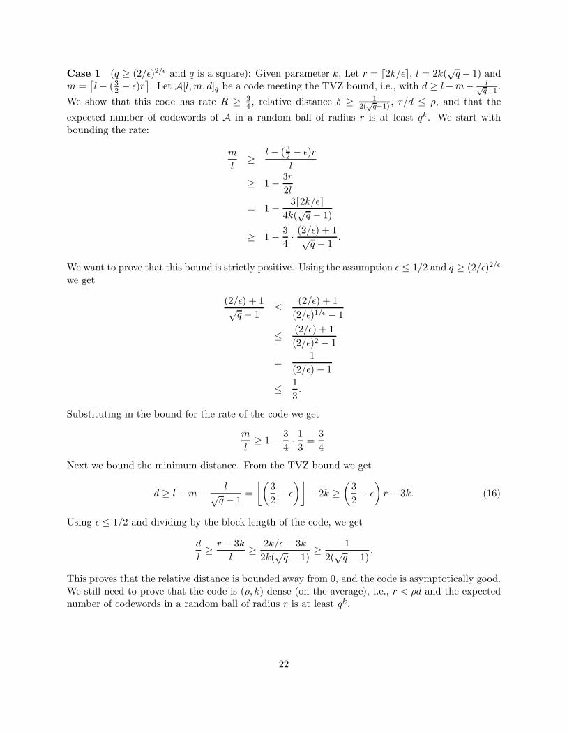
Case 1 (q ≥ (2/ǫ)2/ǫ and q is a square): Given parameter k, Let r = ⌈2k/ǫ⌉, l = 2k(√
q − 1) andm =
⌈l − (3
2 − ǫ)r⌉. Let A[l,m, d]q be a code meeting the TVZ bound, i.e., with d ≥ l−m− l√
q−1 .
We show that this code has rate R ≥ 34 , relative distance δ ≥ 1
2(√
q−1) , r/d ≤ ρ, and that the
expected number of codewords of A in a random ball of radius r is at least qk. We start withbounding the rate:
m
l≥ l − (3
2 − ǫ)r
l
≥ 1 − 3r
2l
= 1 − 3⌈2k/ǫ⌉4k(
√q − 1)
≥ 1 − 3
4· (2/ǫ) + 1√
q − 1.
We want to prove that this bound is strictly positive. Using the assumption ǫ ≤ 1/2 and q ≥ (2/ǫ)2/ǫ
we get
(2/ǫ) + 1√q − 1
≤ (2/ǫ) + 1
(2/ǫ)1/ǫ − 1
≤ (2/ǫ) + 1
(2/ǫ)2 − 1
=1
(2/ǫ) − 1
≤ 1
3.
Substituting in the bound for the rate of the code we get
m
l≥ 1 − 3
4· 1
3=
3
4.
Next we bound the minimum distance. From the TVZ bound we get
d ≥ l − m − l√q − 1
=
⌊(3
2− ǫ
)⌋
− 2k ≥(
3
2− ǫ
)
r − 3k. (16)
Using ǫ ≤ 1/2 and dividing by the block length of the code, we get
d
l≥ r − 3k
l≥ 2k/ǫ − 3k
2k(√
q − 1)≥ 1
2(√
q − 1).
This proves that the relative distance is bounded away from 0, and the code is asymptotically good.We still need to prove that the code is (ρ, k)-dense (on the average), i.e., r < ρd and the expectednumber of codewords in a random ball of radius r is at least qk.
22

We use (16) to bound the ratio d/r.
d
r≥ 3
2− ǫ − 3k
r
≥ 3
2− ǫ − 3k
2k/ǫ
=3
2− 5
2ǫ
>3
2(1 − 2ǫ) =
1
ρ.
This proves that the radius r is small, relative to the minimum distance of the code. We want tobound µm(r), the expected number of codewords in a random ball of radius r. Using (2) and (7),we have
µm(r) ≥(
l
r
)
(q − 1)rqm−l
≥(
l
r
)r
(q − 1)rq−( 32−ǫ)r
≥(
2k(√
q − 1)2kǫ + 1
)r (1√q
)r (
1 − 1
q
)r
qǫr
≥(
ǫ
1 + 1/4
)r (
1 − 1√q
)r (
1 − 1
q
)r
qǫr.
We want to prove that this bound is at least qk. Combining ǫ ≤ 1/2 and q ≥ (2/ǫ)2/ǫ, we getq ≥ 44 = 256. Substituting in the last equation,
µm(r) ≥(
ǫqǫ
5/4
(
1 − 1
256
)(
1 − 1
16
))r
≥( ǫ
2qǫ)2k/ǫ
≥(( ǫ
2
)2/ǫ· q2
)k
≥ qk.
It follows that there exists a vector v such that |B(v, r) ∩A| ≥ qk. This concludes the analysis forlarge square q.
Case 2 (arbitrary q): In this case, let c be the smallest even integer such that q′ = qc ≥ (2/ǫ)2/ǫ.Given k, let A′[l′,m′, d′]q′ be a code and r′ a radius as given in Case 1 with rate m′/l′ ≥ 3
4 , relativedistance d′/l′ ≥ 1/(2(
√q′ − 1)), r′/d′ < ρ and µm′(r′) ≥ (q′)k. We concatenate A′ with equidistant
Hadamard code H[qc − 1, c, qc − qc−1]q to get a code A[l,m, d]q of rate
m
l=
m′cl′(qc − 1)
≥ 3c
4qc> 0,
and relative distanced
l=
d′(qc − qc−1)
l′(qc − 1)≥(
1 − 1
q
)
· 2(√
qc − 1)
>0.
Now given a vector x′ ∈ Fl′
q′ that has (q′)k vectors in the ball of radius r′ around it, the vector
x = x′3H also has (q′)k vectors of A3H in the ball of radius r = (qc − qc−1)r′ around it. Notice
23

that the ratio r/d = r′/d′ does not change in this step, and therefore, r < ρd holds true. This givesthe code as claimed in the proposition. 2
The following lemma stresses the algorithmic components of the code construction above andin particular stresses that we know how to construct the generator matrix of the kth code in thesequence, and how to sample dense balls from this code in polynomial time. (We also added onemore parameter n to the algorithm to ensure that the block length of code A is at least n. Thisadditional parameter will be used in the proofs of Section 7, and is being added for purely technicalreasons related to those proofs.)
Proposition 25 For every prime power q and every ρ > 2/3 , there exist R > 0, δ > 0 and aprobabilistic algorithm that on input three integers k, n and s, outputs (in time polynomial in k, n, s)three other integers l, m, r, a generator matrix A ∈ F
m×lq of a code A and a center v ∈ F
lq (of
weight r) such that
1. m/l ≥ R.
2. d(A)/l ≥ δ.
3. r < ρ · d(A).
4. with probability at least 1 − q−s, the ball B(v, r) contains at least qk codewords of A.
5. l ≥ n.
Proof: Given inputs k, n, s to the algorithm, we consider the (ρ, k′)-dense code Ak′ from Proposi-tion 24, where k′ = max(n, k + s). This code is the concatenation of an algebraic-geometry codeA′[l′,m′, d′]qc and a Hadamard code H[qc−1, c, qc(1−1/q)]q . Therefore a generator matrix A ∈ F
m×lq
for Ak′ can be constructed in time polynomial in k, n, s. Let r′ = ⌊ρd′⌋, r = r′ ·qc · (1−1/q), choosev′ ∈ F
l′qc uniformly at random from B(0, r′) and let v = v′
3H. From the proof of Proposition 24we know that the expected number of codewords in a randomly chosen ball B(v′, r′) is at leastqk+s. We now apply the Lemma 13 instantiating it with groups F = (Fl′
q′ ,+), G = (G,+), and set
B = B(0, r′). Notice that for any center z = z ∈ Fl′
q′ , the set Bz is just the ball B(z, r) of radiusr′ centered in z. From the proof of Proposition 24, the average size of G ∩ Bz (i.e., the expectednumber of codewords in a random ball) is at least qk+s. Setting δ = q−s in Lemma 13, and notingthat B−1 = B = B(0, r′), we immediately get that B(v, r′) contains at least qk codewords withprobability 1−q−s. Finally, by Lemma 10, we get that the corresponding ball B(v, r) in F
lq contains
at least qk codewords from A. 2
We conclude with the following lemma analogous to Lemma 15 of Section 3.
Lemma 26 For every ρ > 2/3 and prime power q, there exist R > 0, δ > 0 and a probabilisticpolynomial time algorithm that on input k, n, s outputs, (in time polynomial in k, n, s), integersl,m, r, and matrices A ∈ F
m×lq , T ∈ F
l×kq and a vector v ∈ F
lq such that:
1. m/l ≥ R.
2. d(A)/l ≥ δ.
3. r < ρ · d(A).
24

4. With probability at least 1 − q−s, T(B(v, r) ∩ A) = Fkq , i.e., for every x ∈ F
kq there exists a
y ∈ A such that d(v,y) ≤ r and yT = x.
5. l ≥ n.
The proof is identical to that of Lemma 15, with the use of Proposition 12 replaced by Propo-sition 25.
7 Hardness results for asymptotically good codes
In this section we prove hardness results for the decoding problem even when restricted to asymp-totically good codes, and the hardness of approximating the minimum distance problem with linear(in the block length) additive error. First, we define a restricted version of GapRNC where thecode is required to be asymptotically good.
Definition 27 For R, δ ∈ (0, 1), let (R, δ)-restricted GapRNC(ρ)γ,q be the restriction of GapRNC
(ρ)γ,q
to instances (A ∈ Fk×nq ,v, t) satisfying k ≥ R · n and t ≥ δ · n.
We call δ relative error weight. Notice that for every constant ρ, the minimum distance of the codesatisfies d > t/ρ ≥ δn/ρ, therefore the code is asymptotically good with information rate at leastk/n ≥ R > 0 and relative distance at least d/n > δ/ρ > 0. In particular, when ρ ≤ 1, the relativedistance is strictly bigger than δ.
In the following subsections, we prove that (R, δ)-restricted GapRNC is NP-hard (under RURreductions). Then we use this result to prove that the minimum distance of a linear code is hardto approximate additively, even to within a linear additive error relative to the block length of thecode. The proofs will be essentially the same as those for non-asymptotically good codes. Themain differences are the following:
• We use the asymptotically good dense code construction from Section 6. Before we relied ondense codes that were not asymptotically good.
• We reduce from a restricted version of the nearest codeword problem in which the error weightis required to be a constant fraction of the block length.
In the following subsection we observe that a result of Hastad [13] gives us hardness of NCPwith this additional property. Then we use this result to prove the hardness of the (R, δ)-restrictedGapRNC problem, and the hardness of GapDistAdd.
7.1 The restricted nearest codeword problem
We define a restricted version of the nearest codeword problem in which the target distance isrequired to be at least a linear fraction of the block length.
Definition 28 For τ ∈ (0, 1), let τ -restricted GapNCPγ,q (τ -GapNCPγ,q for short) be the re-striction of GapNCPγ,q to instances (A ∈ F
k×nq ,v, t) satisfying t ≥ τ · n.
We will need the fact that τ -GapNCPγ,q is NP-hard. This result does not appear to followfrom the proof of [3]. Instead we observe that this result easily follows from a recent and extremelypowerful result of Hastad [13].
25
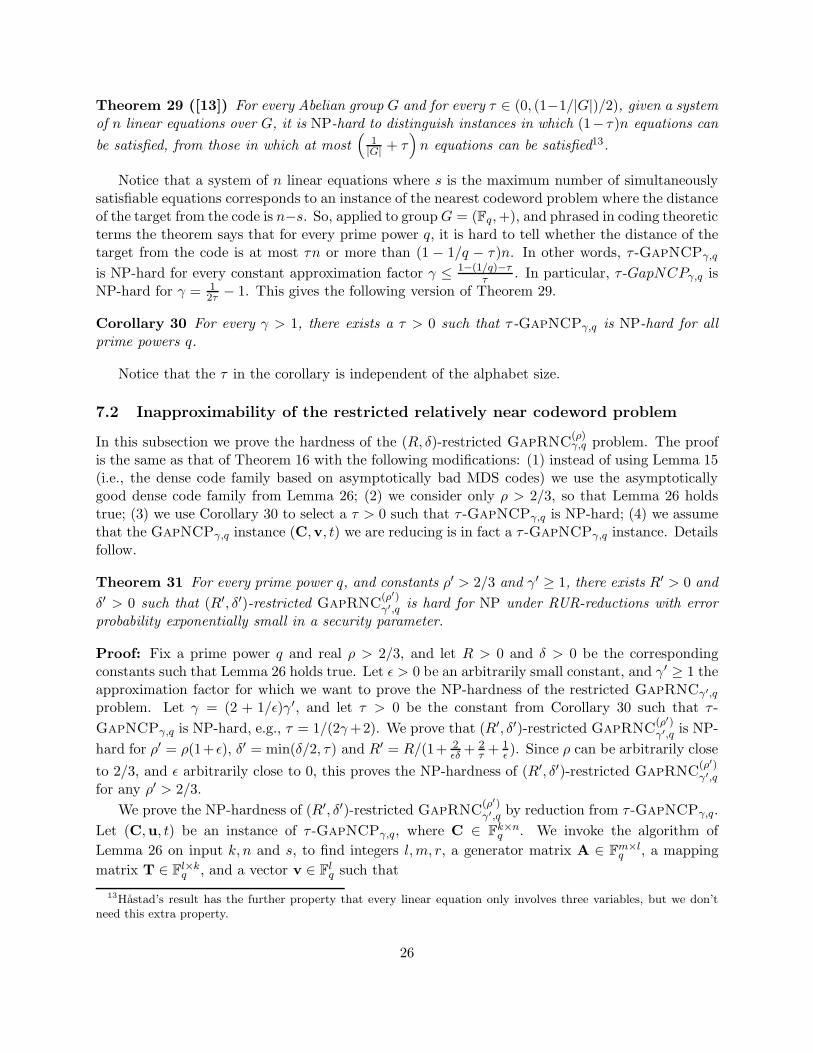
Theorem 29 ([13]) For every Abelian group G and for every τ ∈ (0, (1−1/|G|)/2), given a systemof n linear equations over G, it is NP-hard to distinguish instances in which (1− τ)n equations can
be satisfied, from those in which at most(
1|G| + τ
)
n equations can be satisfied13.
Notice that a system of n linear equations where s is the maximum number of simultaneouslysatisfiable equations corresponds to an instance of the nearest codeword problem where the distanceof the target from the code is n−s. So, applied to group G = (Fq,+), and phrased in coding theoreticterms the theorem says that for every prime power q, it is hard to tell whether the distance of thetarget from the code is at most τn or more than (1 − 1/q − τ)n. In other words, τ -GapNCPγ,q
is NP-hard for every constant approximation factor γ ≤ 1−(1/q)−ττ . In particular, τ -GapNCPγ,q is
NP-hard for γ = 12τ − 1. This gives the following version of Theorem 29.
Corollary 30 For every γ > 1, there exists a τ > 0 such that τ -GapNCPγ,q is NP-hard for allprime powers q.
Notice that the τ in the corollary is independent of the alphabet size.
7.2 Inapproximability of the restricted relatively near codeword problem
In this subsection we prove the hardness of the (R, δ)-restricted GapRNC(ρ)γ,q problem. The proof
is the same as that of Theorem 16 with the following modifications: (1) instead of using Lemma 15(i.e., the dense code family based on asymptotically bad MDS codes) we use the asymptoticallygood dense code family from Lemma 26; (2) we consider only ρ > 2/3, so that Lemma 26 holdstrue; (3) we use Corollary 30 to select a τ > 0 such that τ -GapNCPγ,q is NP-hard; (4) we assumethat the GapNCPγ,q instance (C,v, t) we are reducing is in fact a τ -GapNCPγ,q instance. Detailsfollow.
Theorem 31 For every prime power q, and constants ρ′ > 2/3 and γ′ ≥ 1, there exists R′ > 0 and
δ′ > 0 such that (R′, δ′)-restricted GapRNC(ρ′)γ′,q is hard for NP under RUR-reductions with error
probability exponentially small in a security parameter.
Proof: Fix a prime power q and real ρ > 2/3, and let R > 0 and δ > 0 be the correspondingconstants such that Lemma 26 holds true. Let ǫ > 0 be an arbitrarily small constant, and γ′ ≥ 1 theapproximation factor for which we want to prove the NP-hardness of the restricted GapRNCγ′,q
problem. Let γ = (2 + 1/ǫ)γ′, and let τ > 0 be the constant from Corollary 30 such that τ -
GapNCPγ,q is NP-hard, e.g., τ = 1/(2γ +2). We prove that (R′, δ′)-restricted GapRNC(ρ′)γ′,q is NP-
hard for ρ′ = ρ(1+ ǫ), δ′ = min(δ/2, τ) and R′ = R/(1+ 2ǫδ + 2
τ + 1ǫ ). Since ρ can be arbitrarily close
to 2/3, and ǫ arbitrarily close to 0, this proves the NP-hardness of (R′, δ′)-restricted GapRNC(ρ′)γ′,q
for any ρ′ > 2/3.
We prove the NP-hardness of (R′, δ′)-restricted GapRNC(ρ′)γ′,q by reduction from τ -GapNCPγ,q.
Let (C,u, t) be an instance of τ -GapNCPγ,q, where C ∈ Fk×nq . We invoke the algorithm of
Lemma 26 on input k, n and s, to find integers l,m, r, a generator matrix A ∈ Fm×lq , a mapping
matrix T ∈ Fl×kq , and a vector v ∈ F
lq such that
13Hastad’s result has the further property that every linear equation only involves three variables, but we don’tneed this extra property.
26

1. r < ρ · d(A),
2. for every x ∈ Fkq there exists a y ∈ A satisfying d(v,y) ≤ r and yT = x,
3. m ≥ Rl,
4. d(A) ≥ δl,
5. l ≥ n, and therefore l ≥ t too.
where the second condition holds with probability 1−q−s. Notice that, since any sphere containingmore than a single codeword must have radius at least d(A)/2, the relative radius must be at least
r
l≥ d(A)
2l≥ δ
2.
The reduction proceeds as in the proof of Theorem 16. Let b =⌈
rt
⌉, a =
⌈btǫr
⌉, t′ = ar + bt, and
define code C′ and target u′ as in (10) and (11). The output of the reduction is (C′,u′, t′). Wewant to prove that the map (C,u, t) 7→ (C′,u′, t′) is a valid (RUR) reduction from τ -GapNCPγ,q
to (R′, δ′)-restricted GapRNC(ρ′)γ′,q. The proof of the following facts is exactly the same as in
Theorem 16 (Equations (12), (13) and (14)):
• t′ < ρ′ · d(C′)
• if d(u, C) ≤ t, then d(u′, C′) ≤ t′
• if d(u, C) > γ · t, then d(u′, C′) > γ′ · t′
It remains to prove that GapRNC instance (C′,u′, t′) satisfies the (R′, δ′) restriction. Notice thatthe code C′ has block length n′ = al + bn. Therefore the relative error weight t′/n′ satisfies
t′
n′ =ar + bt
al + bn≥ min
(r
l,
t
n
)
≥ min(δ/2, τ) = δ′.
Finally, the information content of C′ is m, i.e., the same as code A. Therefore, the rate is m/n′ ≥R(l/n′) and in order to show that the code is asymptotically good we need to prove that n′ = O(l).In fact,
a =
⌈bt
ǫr
⌉
≤ 1 +
⌈rt
⌉t
ǫr≤ 1 +
t + r
ǫr≤ 1 +
1
ǫ+
l
ǫr≤ 1 +
1
ǫ+
2
ǫδ
b =⌈r
t
⌉
≤ t + r
t≤ 2l
τn
and
n′ = al + bn ≤(
1 +1
ǫ+
2
ǫδ+
2
τ
)
l.
This proves that the rate of the code is at least
m
n′ ≥R
1 + 1ǫ + 2
ǫδ + 2τ
= R′.
2
27

7.3 Minimum distance with linear additive error
In Lemma 19 we proved that the minimum distance problem is hard to approximate within someconstant factor. The proof was by reduction from GapRNC. The same reduction, when appliedto the restricted GapRNC problem gives an inapproximability result for the minimum distance
problem with linear additive error. In particular, Lemma 19 reduces (R, δ)-restricted GapRNC(ρ)1/ρ,q
to GapDistAddτ,q with τ = δ · ((1/ρ) − 1) > δ · (1 − ρ). This result is formally proved in thefollowing theorem.
Theorem 32 For every prime power q, there exists a τ > 0 such that GapDistAddτ,q is hardfor NP under polynomial RUR-reductions with soundness error exponentially small in a securityparameter.
Proof: The proof is by reduction from (R, δ)-restricted GapRNC(ρ)γ,q with ρ < 1, γ = 1/ρ, and
τ = δ(1 − ρ). The reduction is the same as in the proof of Lemma 19. On input (C,u, t),the reduction outputs (C′, t) where C′ is the code defined in (15). We know from the proof of
Lemma 19 that (C,u, t) 7→ (C′, t) is a valid reduction from GapRNC(ρ)γ,q to GapDistγ,q. We show
that if (C′, t) is a Yes (resp. No) instance of GapDistγ,q, then it is also a Yes (resp. No) instance
of GapDistAddτ,q. This proves that (C,u, t) 7→ (C′, t) is also a valid reduction from GapRNC(ρ)γ,q
to GapDistAddτ,q.The case of Yes instances is trivial, because the definition of Yes instances in GapDistγ,q and
GapDistAddτ,q is the same, namely d(C′) ≤ t. So, assume (C′, t) is a No instance of GapDistγ,q.Then,
d(C′) > γ · t = t +
(1
ρ− 1
)
t ≥ t +
(1
ρ− 1
)
δn ≥ t + τn,
and (C′, t) is a No instance of GapDistAddτ,q. 2
8 Other reductions
We proved that approximating the minimum distance problem is hard for NP under RUR-reductions,i.e. probabilistic reductions that map No instances to No instances, and Yes instances to Yes
instances with high probability. (The same is true for all other reductions presented in this paper,as well as the hardness proof for the shortest vector problem in [2, 18].)
An obvious question is whether it is possible to remove the randomization and make the reduc-tion deterministic. (Observe that a deterministic NP-hardness result is known for the exact versionof the minimum distance problem [23, 22]. In contrast, for the shortest vector problem, even theexact version is known to be NP-hard only under randomized reductions [2].) We notice that ourreductions (as well as the Ajtai-Micciancio ones for SVP) use randomness in a very restricted way.Namely, the only part of the reduction where randomness is used is the proof of Lemma 15 (andLemma 26 for asymptotically good codes). The construction in the lemma depends only on theinput size, and not on the particular input instance we are reducing. So, if the construction suc-ceeds, the reduction will faithfully map all Yes instances (of the appropriate size) to Yes instances.Therefore, the statements in Lemma 15 and Lemma 26 can be easily modified to obtain hardnessresults for NP under deterministic non-uniform reductions, i.e. reductions that take a polynomially
28

sized advice that depends only on the input size14. (The advice is given by the sphere center v andtransformation matrix T satisfying Lemma 15 and Lemma 26.)
Corollary 33 For every finite field Fq the following holds:
• For every ρ > 1/2, and γ ≥ 1 GapRNC(ρ)γ,q is hard for NP under nonuniform polyno-
mial reductions. Therefore, no nonuniform polynomial time (P/poly) algorithm exists for
GapRNC(ρ)γ,q unless NP ⊆ P/poly.
• For every γ > 1, GapDistγ,q is hard for NP under nonuniform polynomial reductions. There-fore, no P/poly algorithm exists for GapDistγ,q unless NP ⊆ P/poly.
• For every ǫ > 0 and γ(n) = 2log(1−ǫ) n, GapDistγ,q is hard for NP under nonuniform quasi-polynomial reductions. Therefore, no nonuniform quasi-polynomial time (QP/poly) algorithmexists for GapDistγ,q unless NP ⊆ QP/poly.
• For every ρ > 1/2, and γ ≥ 1 there exists R > 0 and δ > 0 such that (R, δ)-restricted
GapRNC(ρ)γ,q is hard for NP under nonuniform polynomial reductions. Therefore, no P/poly
algorithm exists for (R, δ)-restricted GapRNC(ρ)γ,q unless NP ⊆ P/poly.
• There exists a τ > 0 such that GapDistAddτ,q is hard for NP under nonuniform polynomialreductions. Therefore, no P/poly algorithm exists for GapDistAddτ,q unless NP ⊆ P/poly.
We notice also that a uniform deterministic construction satisfying the properties of Lemma 15and Lemma 26 would immediately give a proper NP-hardness result (i.e. hardness under deter-ministic Karp reductions) for all problems considered in this paper. Interestingly, for the shortestvector problem, Micciancio [18] (see also [19]) showed that a deterministic NP-hardness result ispossible under a reasonable (but unproven) number theoretic conjecture regarding the distributionof smooth numbers (i.e., numbers with no large prime factors). No deterministic proof under similarnumber theoretic conjectures is known for the coding problems studied in this paper.
Finally, we notice that all our results rely on the fact that the code is given as part of theinput. Thus it is conceivable that for every error-correcting code, there exists a fast algorithm tocorrect errors (say up to the distance of the code), however, this algorithm may be hard to find(given a description of the code). A result along the lines of the one of Bruck and Naor [7], showingthat there are specific sequences of codes for which nearest codewords are hard to find (even ifthe code can be arbitrarily preprocessed) would be desirable to fix this gap in our knowledge.Feige and Micciancio [10] recently showed that the nearest codeword problem with preprocessingis hard to approximate within any factor less than 5/3. Inapproximability results for NCP withpreprocessing are interesting because they can be combined with our reduction (Theorem 16) toprove the inapproximability of RNC with preprocessing. Specifically, Theorem 16 gives a reduction
from GapNCPγ,q to GapRNC(ρ)γ′,q with ρ = (1 + ǫ)/2 and γ′ < γ/(2 + 1/ǫ), with the property
that the GapRNC code depends only on the GapNCP code (and not the target vector). So,
if GapNCPγ,q is hard to solve even when the code can be preprocessed, then also GapRNC(ρ)γ′,q
14Since our reduction achieves exponentially small error probability, hardness under non-uniform reductions also fol-lows from general results about derandomization [1]. However, the ad-hoc derandomization method we just describedis more efficient and intuitive.
29

with preprocessing cannot be efficiently solved. Unfortunately, in order to get non trivial hardness
results for GapRNC(ρ)γ′,q with preprocessing (i.e., results with γ′ ≥ 1) using this method, one
needs to start from inapproximability results for GapNCPγ,q with preprocessing with γ > 2. So,inapproximability factors γ < 5/3 proved in [10] do not suffice. Very recently, the results of [10]have been improved by Regev [20] to γ < 3, giving the first inapproximability results for RNC
(ρ)
with preprocessing. Notice that applying the reduction from Theorem 16 to GapNCPγ,q withγ < 3 allows to establish the inapproximability (within some constant factor γ′ < 3/(2 + 1/ǫ))of GapRNC
(ρ) for ρ = (1 + ǫ)/2. Notice that in order to get γ′ ≥ 1, one needs ǫ > 1, andtherefore ρ > 1. Interestingly, [20] also shows how to modify the reduction in Theorem 16 to getinapproximability of RNC
(ρ) with preprocessing for any ρ > 1/2. The improvement is based onthe following two observations. (The reader is referred to [20] for details.)
1. The lower bound d(C′,u′) ≥ b · d(C,u) in (14) can be strengthened to
d(C′,u′) ≥ a · d(A,v) + b · d(C,u).
2. The center of the sphere v is at distance at least
d(A,v) ≥ min(‖v‖, d(A) − ‖v‖) ≥(
1
ρ− 1
)
r
from the code A.
Based on these two observations, Regev shows that (with a different choice of parameters a and
b) the reduction given in the proof of Theorem 16 maps GapNCPγ,q to GapRNC(ρ)γ′,q for any
γ′ <(
1 − 12ρ
)
γ + 12ρ . Combined with the improved inapproximability results for GapNCP with
preprocessing, this shows that GapRNC(ρ)γ,q with preprocessing is NP-hard (under RUR-reductions
as usual) for any ρ > 1/2 and γ < 3 − 1/ρ.We conclude with a brief discussion of the main problem left open in this work. Our hardness
results for RNC(ρ) hold only for ρ > 1/2. For the case of general (not asymptotically good) codes,
we showed that one can make ρ arbitrarily close to 1/2. However, we cannot achieve equalityρ = 1/2. RNC
(1/2) (also known as the “bounded distance decoding” problem, BDD) is arguablythe most relevant decoding problem in practice, and the one for which most known polynomialtime algorithms (for specific families of codes, e.g., RS codes) work. The problems RNC
(1/2) andRNC
(ρ) for ρ > 1/2 are qualitatively different, because for ρ ≤ 1/2 the solution to the decodingproblem is guaranteed to be unique. Our reduction relies on the construction of a code A and asphere B(v, r) of radius r < ρ ·d(A) such that B(v, r) contains several (in fact, exponentially many)codewords. Clearly, for ρ ≤ 1
2 , no sphere of radius r < ρ · d(A) can contain more than a singlecodeword. So, the bound ρ > 1/2 seems an intrinsic limitation of our reduction technique.15 Weleave determining the computational complexity of BDD as an open problem.
References
[1] L. M. Adleman. Two theorems on random polynomial time. In Proc. 19th Symposium onFoundations of Computer Science, pages 75–83, 1978.
15The same problem on integer lattices is also the current bottleneck to extend the inapproximability factor of theshortest vector problem beyond
√2 [18].
30

[2] M. Ajtai. The shortest vector problem in L 2 is NP-hard for randomized reductions (extendedabstract). In Proceedings of the 30th Annual ACM Symposium on Theory of Computing, pages10–19, Dallas, Texas, May 23–26 1998.
[3] S. Arora, L. Babai, J. Stern, and E. Z. Sweedyk. The hardness of approximate optima inlattices, codes, and systems of linear equations. J. Comput. Syst. Sci., 54(2):317–331, Apr.1997. Preliminary version in FOCS’93.
[4] S. Arora and C. Lund. Approximation algorithms for NP-hard problems, chapter 10, Hardnessof Approximation. PWS Publishing, Boston, 1996.
[5] E. Berlekamp, R. McEliece, and H. van Tilborg. On the inherent intractability of certaincoding problems. IEEE Transactions on Information Theory, 24(3):384–386, 1978.
[6] P. Berman and M. Karpinski. Approximating minimum unsatisfiability of linear equations. InProceedings of the 13th annual ACM-SIAM Symposium on Discrete Algorithms, SODA ’02,pages 74–83, San Francisco, California, 2002.
[7] J. Bruck and M. Naor. The hardness of decoding linear codes with preprocessing. IEEETransactions on Information Theory, 36(2):381–385, Mar. 1990.
[8] I. Dinur, G. Kindler, R. Raz, and S. Safra. An improved lower bound for approximating CVP.Manuscript, 1999.
[9] I. Dinur, G. Kindler, and S. Safra. Approximating CVP to within almost-polynomial factors isNP-hard. In 39th annual symposium on foundations of computer science, Palo Alto, California,Nov. 7–10 1998. IEEE.
[10] U. Feige and D. Micciancio. The inapproximability of lattice and coding problems with pre-processing. In IEEE Conference on Computational Complexity - CCC 2002, pages 44–52,Montreal, Canada, May 21–23 2002. IEEE.
[11] G. D. Forney Jr. Concatenated codes. Number 37 in Research Monograph. MIT Press, Cam-bridge, Massachusetts, 1966.
[12] J. Hastad. Clique is hard to approximate within n1−ǫ. Acta Mathematica, 182:105–142, 1999.
[13] J. Hastad. Some optimal inapproximability results. Journal of ACM, 48:798–859, 2001. Pre-liminary version in Proc. of STOC’97.
[14] K. Jain, M. Sudan, and V. Vazirani. Personal communication, May 1998.
[15] D. S. Johnson. Handbook of Theoretical Computer Science, volume A (Algorithms and Com-plexity), chapter 2, A catalog of complexity classes, pages 67–161. Elsevier, 1990.
[16] J. Justesen and T. Høholdt. Bounds on list decoding of MDS codes. IEEE Transactions onInformation Theory, 47(4):1604–1609, May 2001.
[17] F. MacWilliams and N. Sloane. The theory of error-correcting codes. North-Holland, Amster-dam, The Netherlands, 1981.
31

[18] D. Micciancio. The shortest vector problem is NP-hard to approximate to within some con-stant. SIAM Journal on Computing, 30(6):2008–2035, Mar. 2001. Preliminary version in FOCS1998.
[19] D. Micciancio and S. Goldwasser. Complexity of Lattice Problems: a cryptographic perspective,volume 671 of The Kluwer International Series in Engineering and Computer Science. KluwerAcademic Publishers, Boston, Massachusetts, Mar. 2002.
[20] O. Regev. Improved inapproximability of lattice and coding problems with preprocessing.Manuscript, Aug. 2002.
[21] M. Tsfasman and S. Vladut. Algebraic-Geometric Codes. Kluwer, Dordrecht, 1991.
[22] A. Vardy. Algorithmic complexity in coding theory and the minimum distance problem. InProceedings of the twenty-ninth annual ACM Symposium on Theory of computing, STOC’97,pages 92–109, El Paso, Texas, May 4–6 1997. ACM.
[23] A. Vardy. The intractability of computing the minimum distance of a code. IEEE Transactionson Information Theory, 43(6):1757–1766, Nov. 1997.
[24] V. Zinoviev and S. Litsyn. On codes exceeding the gilbert bound. Problems of InformationTransmission, 21(1):109–111, 1985. (in Russian).
32