Hard Mathematics Applied to Soft Decisions

Thomas L. Saaty

1. IntroductionNearly all of us have been brought up to believe that clear-headed logical thinking is our only sure way to face and solve problems. But experience suggests that logical thinking is not natural to us. Indeed, we have to practice, and for a long time, before we can do it well. Since complex problems usually have many related factors, traditional logical thinking leads to sequences of ideas so tangled that the best solution cannot be easily discerned.

A common kind of decision problem we face is something like this: Suppose one wishes to buy a house. The different houses being considered have some attributes or criteria in common that are important to the decision-maker. If one house were best on every criterion the choice would be easy, but usually the house that is best on one criterion (e.g., cost) is worst on another (e.g., size). How should one make the tradeoff? We describe and discuss a mathematical model, the Analytic Hierarchy Process (AHP) that can be used to make such decisions.

2. Choosing the Best HouseConsider the following (hypothetical) example: a family wishing to purchase a house identifies eight criteria that are important to them. The problem is to select one of three candidate houses. The first step is to structure the problem into a hierarchy (see Figure 1). On the first (top) level is the overall goal of Satisfaction with House. On the second level are the eight criteria that contribute to the goal, and on the third (bottom) level are the three candidate houses that are to be evaluated by considering the criteria on the second level.

The criteria important to the family are:1. Size of House: Storage space; size of rooms; number of rooms; total area of house.2. Transportation: Convenience and proximity of bus service.3. Neighborhood: Degree of traffic, security, taxes, physical condition of surrounding

buildings.4. Age of House: How long ago house was built.5. Yard Space: Front, back, and side space, and space shared with neighbors.6. Modern Facilities: Dishwasher, garbage disposal, air conditioning, alarm system, and

other such items.7. General Condition: Extent to which repairs are needed; condition of walls, carpet, drapes,

wiring; cleanliness.8. Financing: Availability of assumable mortgage, seller financing, or bank financing.

1

Figure 1. Decomposition of the Problem into a Hierarchy.

The next step is to make comparative judgments. The family assesses the relative importance of all possible pairs of criteria with respect to the overall goal, Satisfaction with House, coming to a consensus judgment on each pair, and their judgments are arranged into a matrix. The question to ask when comparing two criteria is: which is more important and how much more important is it with respect to satisfaction with a house?

The matrix of pairwise comparison judgments on the criteria given by the home-buyers in this case is shown in Table 1. The judgments are entered using the fundamental scale of the AHP: a criterion compared with itself is always assigned the value 1 so the main diagonal entries of the pairwise comparison matrix are all 1. The numbers 3, 5, 7, and 9 correspond to the verbal judgments “moderately more dominant”, “strongly more dominant”, “very strongly more dominant”, and “extremely more dominant” (with 2, 4, 6, and 8 for compromise between the previous values). Reciprocal values are automatically entered in the transpose position, so the family must make a total of 28 pairwise judgments. We are permitted to interpolate values between the integers, if desired.

In the AHP model, the vector of priorities for the criteria is obtained by computing the principal eigenvector, the classical Perron vector, of the pairwise comparison matrix. Because the pairwise comparison matrix has positive entries, the Perron-Frobenius Theorem ensures that there is a unique positive vector (denoted by w) whose entries sum to one that is an eigenvector of the pairwise comparison matrix, and it is associated with an eigenvalue (denoted by ¸ max) of strictly largest modulus. That eigenvalue, the Perron eigenvalue, is positive and algebraically simple (multiplicity one as a root of the characteristic equation) [3, Theorem 8.2.11] . Consistency of the family’s set of judgments is measured by the consistency ratio (C.R.), which we explain later.

2

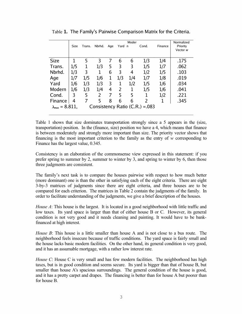
Table 1. The Family’ s Pairwise Comparison Matrix for the Criteria.

Size Trans. Nbrhd. Age Yard Modern Cond. Finance

Normalized Priority

Vector w

SizeTrans.Nbrhd.AgeYardModernCond.Finance

11/51/31/71/61/634

513

1/51/31/357

31/31

1/61/31/425

75613478

633

1/31256

634

1/41/2156

1/31/51/21/71/51/512

1/41/71/51/81/61/61/21

.175

.062

.103

.019

.034

.041

.221

.345¸max = 8.811, Consistency Ratio (C.R.) =.083

Table 1 shows that size dominates transportation strongly since a 5 appears in the (size, transportation) position. In the (finance, size) position we have a 4, which means that finance is between moderately and strongly more important than size. The priority vector shows that financing is the most important criterion to the family as the entry of w corresponding to Finance has the largest value, 0.345.

Consistency is an elaboration of the commonsense view expressed in this statement: if you prefer spring to summer by 2, summer to winter by 3, and spring to winter by 6, then those three judgments are consistent.

The family’s next task is to compare the houses pairwise with respect to how much better (more dominant) one is than the other in satisfying each of the eight criteria. There are eight 3-by-3 matrices of judgments since there are eight criteria, and three houses are to be compared for each criterion. The matrices in Table 2 contain the judgments of the family. In order to facilitate understanding of the judgments, we give a brief description of the houses.

House A: This house is the largest. It is located in a good neighborhood with little traffic and low taxes. Its yard space is larger than that of either house B or C. However, its general condition is not very good and it needs cleaning and painting. It would have to be bank-financed at high interest.

House B: This house is a little smaller than house A and is not close to a bus route. The neighborhood feels insecure because of traffic conditions. The yard space is fairly small and the house lacks basic modern facilities. On the other hand, its general condition is very good, and it has an assumable mortgage, with a rather low interest rate.

House C: House C is very small and has few modern facilities. The neighborhood has high taxes, but is in good condition and seems secure. Its yard is bigger than that of house B, but smaller than house A's spacious surroundings. The general condition of the house is good, and it has a pretty carpet and drapes. The financing is better than for house A but poorer than for house B.

3

Table 2. Pairwise Comparison Matrices for the Alternative Houses Size

of House A B CDistributive Priorities

Idealized Priorities

Yard Space A B C

Distributive Priorities

Idealized Priorities

ABC

11/51/9

51

1/4

941

.743

.194

.063

1.0000.2610.085

ABC

11/61/4

613

41/31

.691

.091

.218

1.0000.1320.315

C.R. = .07 C.R. = .05Transportatio

n A B CDistributive Priorities

Idealized Priorities

Modern Facilities A B C

Distributive Priorities

Idealized Priorities

ABC

11/45

419

1/51/91

.194

.063

.743

0.2610.0851.000

ABC

11/91/6

913

61/31

.770

.068

.162

1.0000.0880.210

C.R. = .07 C.R. = .05Neighborhood

A B CDistributive Priorities

Idealized Priorities

GeneralCondition A B C

Distributive Priorities

Idealized Priorities

ABC

11/91/4

914

41/41

.717

.066

.217

1.0000.0920.303

ABC

122

1/211

1/211

.200

.400

.400

0.5001.0001.000

C.R. = .04 C.R. = .00Age of House

A B CDistributive Priorities

Idealized Priorities

FinancingA B C

Distributive Priorities

Idealized Priorities

ABC

111

111

111

.333

.333

.333

1.0001.0001.000

ABC

175

1/71

1/3

1/531

.072

.650

.278

0.1111.0000.430

C.R. = .00 C.R. = .06

In Table 2 both ordinary (distributive) and idealized priority vectors of the three houses are given for each of the criteria. The idealized priority vector is obtained by dividing each element of the distributive priority vector by its largest element. The composite priority vector for the houses is obtained by multiplying each priority vector by the priority of the corresponding criterion, adding across all the criteria for each house and then normalizing. When we use the (ordinary)distributive priority vectors, this method of synthesis is known as the distributive mode and yields A= .345, B= .369, and C= .285. Thus house B is preferred to houses A and C in the ratios: .369/ .346 and .369/ .285, respectively.

When we use the idealized priority vector the synthesis is called the ideal mode. This yields A= .315, B= .383, C= .302 and B is again the most preferred house. The two ways of synthesizing are shown in Table 3.

4

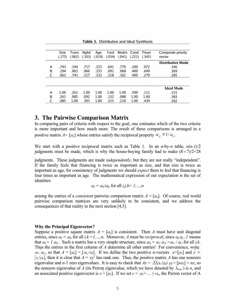
Table 3. Distributive and Ideal Synthesis

Size(.175)

Trans(.062)

Nghd (.103)

Age(.019)

Yard(.034)

Modrn(.041)

Cond(.221)

Finan(.345)

Composite priority vector

ABC

.743

.194

.063

.194

.063

.743

.717

.066

.217

.333

.333

.333

.691

.091

.218

.770

.068

.162

.200

.400

.400

.072

.649

.279

Distributive Mode.346.369.285

ABC

1.00.261.085

.261

.0851.00

1.00.092.303

1.001.001.00

1.00.132.315

1.00.088.210

.5001.001.00

.1111.00.430

Ideal Mode.315.383.302

3. The Pairwise Comparison MatrixIn comparing pairs of criteria with respect to the goal, one estimates which of the two criteria is more important and how much more. The result of these comparisons is arranged in a positive matrix A= [aij] whose entries satisfy the reciprocal property ijji aa /1= .

We start with a positive reciprocal matrix such as Table 1. In an n-by-n table, n(n-1)/2 judgments must be made, which is why the house-buying family had to make (8£7)/2=28

judgments. These judgments are made independently, but they are not really “independent”. If the family feels that financing is twice as important as size, and that size is twice as important as age, for consistency of judgments we should expect them to feel that financing is four times as important as age. The mathematical expression of our expectation is the set of identities

aij = aik/ajk, for all i,j,k= 1,…,n

among the entries of a consistent pairwise comparison matrix A = [aij]. Of course, real world pairwise comparison matrices are very unlikely to be consistent, and we address the consequences of that reality in the next section [4,5].

Why the Principal Eigenvector?Suppose a positive square matrix A = [aij] is consistent. Then A must have unit diagonal entries, since aii = aik, for all i,k =1,…,n. Moreover, A must be reciprocal, since aij aji =1 means that aij = 1/ aji . Such a matrix has a very simple structure, since aik = ai1 a1k =ai1 / ak1 for all i,k. Thus the entries in the first column of A determine all other entries! For convenience, write ®i= ai1, so that A = [aij] = [ ®i /®j]. If we define the two positive n-vectors x=[®i] and y =

[1=®i], then it is clear that A = xyT has rank one. Thus, the positive matrix A has one nonzero eigenvalue and n-1 zero eigenvalues. It is easy to check that Ax = §(®i /®j) ®j = [n®i] = nx, so the nonzero eigenvalue of A (its Perron eigenvalue, which we have denoted by ¸max ) is n, and an associated positive eigenvector is x = [®i]. If we set c = ®1+… +®n, the Perron vector of A

5

(its unique positive eigenvector whose entries sum to one) may be written as w = x/c = [®i/c] [wi]. The Perron vector determines all the entries of A: A= [aij] = [®i /®j] = [(®i /c)/(®j/c)] = [wi/ wj].

We know that an n-by-n positive consistent matrix A = [aij] has a unique positive eigenvector w [wi] (its Perron vector) whose entries sum to one and whose corresponding eigenvalue (its Perron eigenvalue) is n. Moreover, the ratios of the entries of w are precisely the entries of A: aij = wi/ wj. If we think of A as a matrix of (perfectly) consistent pairwise comparisons for n given elements, then the n values wi are a natural set of priorities that underlie the set of pairwise judgments: aij = wi/ wj.

The foregoing discussion is intended to motivate the central and critical choice of the Perron vector as the means to extract a vector of priorities from a given pairwise comparison matrix in the AHP model. If humans made perfectly consistent judgments all the time, the model would be perfect. But they do not, so we must now face the question of assessing the deviation from consistency of an actual pairwise comparison matrix and the consequences of inconsistency for the quality of decisions made according to the AHP model.

4. When is a Positive Reciprocal Matrix Consistent?

Let A= [aij] be an n-by-n positive reciprocal matrix, so all aii =1 and aij =1/ aji for all i,j=1,…,n. Let w = [wi] be the Perron vector of A, let D = diag (w1, ..., wn) be the n-by-n diagonal matrix whose main diagonal entries are the entries of w, and set E = D-1AD = [aij wj /wi] = [°ij]. Then E is similar to A and is a positive reciprocal matrix since °ji = ajiwi/wj = (aij wj /wi)-1 = 1/°ij . Moreover, all the row sums of E are equal to the Perron eigenvalue of A:

maxmax1

//][/ λλε ==== ∑∑=

iiiiijj ij

n

jij wwwAwwwa

.

The computation

22

1,

1

1,11 1max 2/)()()()( nnnnnn

n

jiji

ijijji

n

jiji

ij

n

iii

n

i

n

jij =−+≥++=++== ∑∑∑∑ ∑

≠=

−

≠=== =

εεεεεελ (1)

reveals that .max n≥λ Moreover, since 2/1 ≥+ xx for all x > 0, with equality if and only

if x = 1, we see that n=maxλ if and only if all °ij = 1, which is equivalent to having all aij = wi/ wj.

The foregoing arguments show that a positive reciprocal matrix A has n≥maxλ , with equality if and only if A is consistent. As our measure of deviation of A from consistency, we choose the consistency index

.1

max

−−

≡n

nλµ

6

We have seen that 0≥µ and 0=µ if and only if A is consistent. These two desirable properties explain the term “n” in the numerator of µ ; what about the term “n-1” in the

denominator? Since trace A = n is the sum of all the eigenvalues of A, if we denote the

eigenvalues of A that are different from maxλ by 12 ,..., −nλλ , we see that ∑=

+=n

iin

2max λλ , so

∑=

=−n

iin

2max λλ and ∑

=−=

n

iin 11

1 λµ is the average of the non-Perron eigenvalues of A.

It is an easy, but instructive, computation to show that 2max =λ for every 2-by-2 positive reciprocal matrix:

− 1

11α

α

+

+=

+

+−− 11 )1(

12

)1(

1

ααα

ααα

Thus, every 2-by-2 positive reciprocal matrix is consistent.

Not every 3-by-3 positive reciprocal matrix is consistent, but in this case we are fortunate to have again explicit formulas for the Perron eigenvalue and eigenvector. For

=

1/1/1

1/1

1

cb

ca

ba

A ,

we have 1max 1 −++= ddλ , 3/1)/( bacd = and

)1/(1 d

cbdbdw ++= , )1(/2 d

cbddcw ++= , )1/(13 d

cbdw ++= . (2)

Note that 3max =λ when d = 1 or c = b/a, which is true if and only if A is consistent.

In order to get some feel for what the consistency index might be telling us about a positive n-by-n reciprocal matrix A, consider the following simulation: choose the entries of A above the main diagonal at random from the 17 values {1/9, 1/8,…,1/2, 1, 2,…,8, 9}. Then fill in the entries of A below the diagonal by taking reciprocals. Put ones down the main diagonal and compute the consistency index. Do this 50,000 times and take the average, which we call the random index. Table 4 shows the values obtained from one set of such simulations, for matrices of size 1, 2,…,10.

Table 4. Random Index

n 1 2 3 4 5 6 7 8 9 10

Random Index 0 0 .52 .89 1.11 1.25 1.35 1.40 1.45 1.49

7

Since it would be pointless to try to discern any priority ranking from a set of random comparison judgments, we should probably be uncomfortable about proceeding unless the consistency index of a pairwise comparison matrix is very much smaller than the corresponding random index value in Table 4. The consistency ratio (C.R.) of a pairwise comparison matrix is the ratio of its consistency index ¹ to the corresponding random index value in Table 4.

As a rule of thumb, we do not recommend proceeding if the consistency ratio is more than about .10 for n ¸ 4. For n = 3, we recommend that the C.R. be less than .05.

If the C.R. is larger than desired, we do three things: 1) Find the most inconsistent judgment in the matrix, 2) Determine the range of values to which that judgment can be changed corresponding to which the inconsistency would be improved, 3) Ask the family to consider, if they can, changing their judgment to a plausible value in that range. If they are unwilling, we try with the second most inconsistent judgment and so on. If no judgment is changed the decision is postponed until better understanding of the criteria is obtained. In our house example the family initially made a judgment of 6 for the 37a entry in Table 1 and the consistency index of the set of judgments was ¹ = (9.669 – 8)/7 = .238. But C.R. = .238/1.40 = .17 is higher than the recommended value of .10. If we are going to ask the family to reconsider, and perhaps change, some of their pairwise comparisons, where should we start?

Four methods are plausible for this purpose, and two of them have been implemented in software. All require theoretical investigation of convergence and efficiency. The first uses an explicit formula for the partial derivatives of the Perron eigenvalue with respect to the matrix entries.

For a given positive reciprocal matrix A= [aij] and a given pair of distinct indices k > l, define A(t)= [aij(t)] by akl(t) ´ akl + t, alk(t) ´ (alk + t) –1, and aij(t) ´aij for all i_≠ k, j≠ l , so A(0) =

A. Let maxλ (t) denote the Perron eigenvalue of A(t) for all t in a neighborhood of t = 0 that is small enough to ensure that all entries of the reciprocal matrix A(t) are positive there. Finally, let v = [vi] be the unique positive eigenvector of the positive matrix AT that is normalized so that vTw = 1. Then a classical perturbation formula [3, theorem 6.3.12] tells us that

wAvwv

wAv

dt

td TT

T

t

)0(')0(')(

0

max ===

λ.

12 klkl

lk wva

wv −=

We conclude that

ijjijiij

wvawva

2max −=∂

∂λ for all i,j=1,…,n. (3)

8

Because we are operating within the set of positive reciprocal matrices, =∂

∂

jiamaxλ

-ija∂

∂ maxλ

for all i and j.Thus, to identify an entry of A whose adjustment within the class of reciprocal matrices would result in the largest rate of change in maxλ (and hence in ) we should examine the n(n-1)/2

values jiwvawv ijjiji >− },{ 2and select (any) one of largest absolute value. For the pairwise

comparison matrix in Table 1, v = (.042, .114, .063, .368, .194, .168, .030, .021)T. Table 5

gives the array of partial derivatives (3) for the matrix of criteria in Table 1 with 37a = 6.

Table 5: Partial Derivatives for the House ExampleSize Trans. Nbrhd. Age Yard Modern Cond. Finance

Size - 0.032885 0.056378 -0.009009 0.008752 0.016702 -0.686161 -0.777949Trans. - - -0.427761 0.02325 0.045492 0.064006 -0.38795 -0.421008Nbrhd. - - - 0.003075 -0.00144 0.027725 0.028884 -0.564602Age - - - - -0.384938 -0.663086 0.954093 1.835323Yard - - - - - -0.266026 0.315209 0.757916Modern - - - - - - 0.109645 0.494418Cond. - - - - - - - -0.141185Finance - - - - - - - -

The (4,8) entry in Table 5 is largest in absolute value. Thus, the family could be asked to reconsider their judgment (4,8) of Age vs. Finance. One can then repeat this process with the goal of bringing the C.R within the desired range. If the indicated judgments cannot be changed fully according to one’s understanding, they can be changed partially. Failing the attainment of a consistency level with justifiable judgments, one needs to learn more before proceeding with the decision.

The other three methods, presented here in order of increasing observed efficiency in practice, are conceptually different. They are based on our earlier observation (1) that

).(1,

1max ∑

≠=

−+=−n

jiji

ijijnn εελ

This suggests that we examine the judgment for which ij is farthest from one, that is, an entry aij for which aij wj / wi is the largest, and see if this entry can reasonably be made smaller. We hope that such a change of aij also results in a new comparison matrix with smaller Perron eigenvalue. To demonstrate how improving judgments works, let us return the house example matrix in Table 1. The family first gave a judgment of 6 for the a37

entry. This caused the matrix to have C.R. = .17, which is high. To identify an entry ripe for consideration, construct the matrix °ij (Table 6). The largest value in Table 6 is 5.32156, which focuses attention on a37 = 6.

Table 6: °ij = aij wj/wi

9

1.00000 1.55965 3.26120 0.70829 1.07648 1.25947 0.32138 0.481430.64117 1.00000 1.16165 1.62191 1.72551 2.01882 0.61818 0.881940.30664 0.86084 1.00000 0.55848 0.49513 0.77239 5.32156 0.354301.41185 0.61656 1.79056 1.00000 0.59104 0.51863 1.36123 2.378990.92895 0.57954 2.01967 1.69193 1.00000 0.58499 1.07478 1.788930.79399 0.49534 1.29467 1.92815 1.70942 1.00000 0.91862 1.529013.11156 1.61765 2.25498 0.73463 0.93042 1.08858 1.00000 0.998682.07712 1.13386 2.82246 0.42035 0.55899 0.65402 1.00133 1.00000

How does one determine the most consistent entry for the (3,7) position? When we compute the new eigenvector w after changing the (3,7) entry, we want the new (3,7) entry to be w3 / w7 and the new (7,3) to be w7 /w3 . On replacing a37 by w3 / w7 and a73 by w7 / w3 and multiplying by the vector w one obtains the same product as one would by replacing a37 and a73 by zeros and the two corresponding diagonal entries by two. We take the Perron vector of the latter matrix to be our w and use the now-known values of w3 / w7 and w7 / w3 to replace a37 and a73 in the original matrix [2].The family is now invited to change their judgment towards this new value of a37 as much as they can. Here the value was a37 = 1/ 2.2, approximated by 1/ 2 from the AHP integer valued scale and we hypothetically changed it to 1/2 to illustrate the procedure. If the family does not wish to change the original value of a37, one considers the second most inconsistent judgment and repeats the process. The procedure just described is used in the AHP software Expert Choice.

A refinement of this approach is due to W. Adams. One by one, each reciprocal pair aij and aji

in the matrix is replaced by zero and the corresponding diagonal entries aii and ajj are replaced by 2, the Perron eigenvalue maxλ is computed. The entry with the largest resulting maxλ is identified for change as described above. This method, unpublished, is in use in the Analytic Network Process (ANP) software program [6].

5. Alternative Ways to Determine a Priority VectorSeveral ways, other than the Perron eigenvector method (EM), have been proposed to associate a priority vector with a given positive reciprocal matrix A.

The method of least squares (LSM) determines a priority vector by minimizing the Frobenius norm of the difference between A and a positive rank one reciprocal matrix [yi /yj]:

2

1,0

)/(min j

n

jiiij

yyya∑

=

−

(4)

The method of logarithmic least squares (LLSM) determines a priority vector by minimizing the Frobenius norm of [log (aij xj /xi)]:

2

1,0

)]/log([logmin j

n

jiiij

xxxa∑

=

−

All three methods –EM, LSM, and LLSM– produce the same priority vector when A is consistent. In general, the three methods give different priority vectors and different rankings. Here is an example:

EM = LLSM LSM

10

17/15/1

712/1

521

077.

382.

541.

076.

514.

410.

LSM does not always yield a unique priority vector. In this case, a second LSM solution is (.779, .097, .124); both solutions yield the minimum value 71.48 for (4).

Remarkably, a straightforward calculation (differentiate and equate to zero) gives an analytic expression for the normalized LLSM priority vector, which is unique:

.,...,1,)(/)( /1

1 11

/1 niaax nn

iij

n

j

n

j

niji == ∑ ∏∏

= ==

A computation reveals that for n = 3, this priority vector coincides with that of EM given in (2).

However, the following example shows that for n > 3, the priority vector and criteria rankings produced by EM and LLSM need not be the same.

EM LLSM

15/15/18/12/1

51418

54/113/12

81317

28/12/17/11

043.

387.

134.

374.

061.

042.

380.

133.

384.

062.

(5)

EM ranks the fourth criterion above the second, while LLSM ranks the second above the fourth. LLSM simply takes the normalized values of the 5th roots of the products of the entries in each row without regard to the numerical relation of these elements to other entries in the matrix.

But there is more to a priority vector than uniqueness. When A = [ i /j] is consistent, then Ak

= nk-1A. This says that how much a criterion represented by a row of A dominates other criteria through chains of k arcs is uniquely determined by the single arc chains represented by the rows of A itself. But this is not true when A is inconsistent.

Criterion i is said to dominate criterion j in one step, if the sum of the entries in row i of A is greater than the sum of the entries in row j. It is convenient to use the vector e = (1,…,1)T

to express this dominance: Criterion i dominates criterion j in one step if (Ae)i> (Ae)j . A criterion can dominate another criterion in more than one step by dominating other criteria that in turn dominate the second criterion. Two-step dominance is identified by squaring the matrix and summing its rows, three-step dominance by cubing it, and so on. Thus, criterion i dominates criterion j in k steps if if (Ake)i> (Ake)j . Criterion i is said simply to dominate criterion j if entry i of the vector

11

eAeeAm

kTm

i

k

m∑

=∞→1

/1

lim (6)

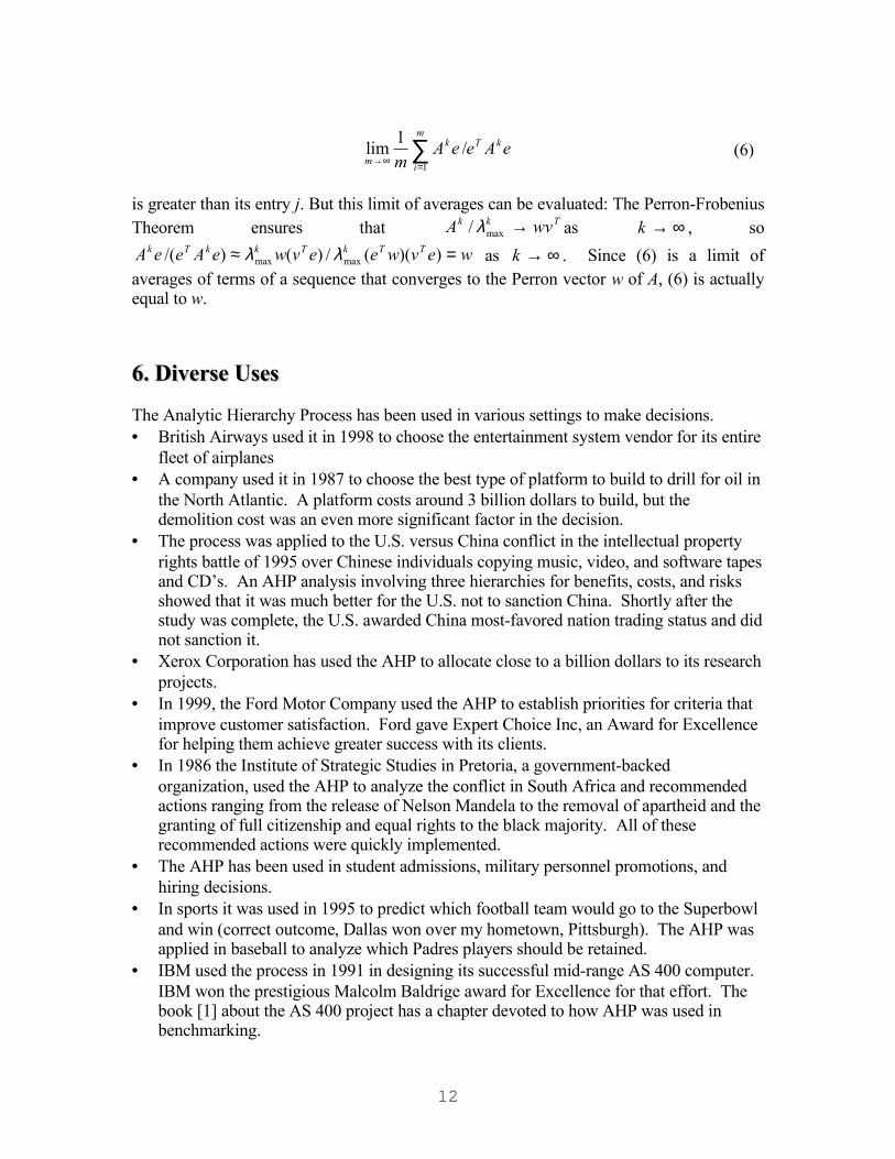
is greater than its entry j. But this limit of averages can be evaluated: The Perron-Frobenius Theorem ensures that Tkk wvA →max/ λ as ∞→k , so

wevweevweAeeA TTkTkkTk =≈ ))((/)()/( maxmax λλ as ∞→k . Since (6) is a limit of averages of terms of a sequence that converges to the Perron vector w of A, (6) is actually equal to w.

6. Diverse Uses6. Diverse Uses

The Analytic Hierarchy Process has been used in various settings to make decisions.• British Airways used it in 1998 to choose the entertainment system vendor for its entire

fleet of airplanes• A company used it in 1987 to choose the best type of platform to build to drill for oil in

the North Atlantic. A platform costs around 3 billion dollars to build, but the demolition cost was an even more significant factor in the decision.

• The process was applied to the U.S. versus China conflict in the intellectual property rights battle of 1995 over Chinese individuals copying music, video, and software tapes and CD’s. An AHP analysis involving three hierarchies for benefits, costs, and risks showed that it was much better for the U.S. not to sanction China. Shortly after the study was complete, the U.S. awarded China most-favored nation trading status and did not sanction it.

• Xerox Corporation has used the AHP to allocate close to a billion dollars to its research projects.

• In 1999, the Ford Motor Company used the AHP to establish priorities for criteria that improve customer satisfaction. Ford gave Expert Choice Inc, an Award for Excellence for helping them achieve greater success with its clients.

• In 1986 the Institute of Strategic Studies in Pretoria, a government-backed organization, used the AHP to analyze the conflict in South Africa and recommended actions ranging from the release of Nelson Mandela to the removal of apartheid and the granting of full citizenship and equal rights to the black majority. All of these recommended actions were quickly implemented.

• The AHP has been used in student admissions, military personnel promotions, and hiring decisions.

• In sports it was used in 1995 to predict which football team would go to the Superbowl and win (correct outcome, Dallas won over my hometown, Pittsburgh). The AHP was applied in baseball to analyze which Padres players should be retained.

• IBM used the process in 1991 in designing its successful mid-range AS 400 computer. IBM won the prestigious Malcolm Baldrige award for Excellence for that effort. The book [1] about the AS 400 project has a chapter devoted to how AHP was used in benchmarking.

12

Since the AHP helps one organize one’s thinking, it can be used to deal with many decisions that are often made intuitively. At a minimum the process allows one to experiment with different criteria and different judgments. A trial version of the AHP software can be obtained from www.expertchoice.com. The ANP software is an alpha version obtainable on www.creativedecisions.net.

References

1. R.A. Bauer, E. Collar, and V. Tang, The Silverlake Project, Oxford University Press, New York,1992.

2. P. T. Harker, Derivatives of the Perron Root of a Positive Reciprocal Matrix: With Applications to the Analytic Hierarchy Process, Appl. Math. Comput. 22 (1987) 217-232.

3. R.A. Horn and C.R. Johnson, Matrix Analysis, Cambridge University Press, New York,1985.4. T.L. Saaty, The Analytic Hierarchy Process, McGraw Hill, New York, 1980. Reprinted by RWS Publications, 4922 Ellsworth Avenue, Pittsburgh, PA, 15213, 2000.

5. T.L. Saaty, Fundamentals of Decision Making with the Analytic Hierarchy Process, RWS Publications, 4922 Ellsworth Avenue, Pittsburgh, PA, 15213, 2000.

6. T.L. Saaty, Decision Making with Dependence and Feedback: The Analytic Network Process, RWS Publications, 4922 Ellsworth Avenue, Pittsburgh, PA, 15213, 1996.

University of Pittsburgh, 322 Mervis Hall, Pittsburgh, PA. 15260. saaty@katz.pitt.edu

13