hanson’s market scoring rules
DESCRIPTION
Hanson’s Market Scoring Rules. Robin Hanson, Logarithmic Market Scoring Rules for Modular Combinatorial Information Aggregation , 2002. Robin Hanson, Combinatorial Information Market Design , 2003. Proper Scoring Rules. - PowerPoint PPT PresentationTRANSCRIPT

Hanson’s Market Scoring Rules
Robin Hanson, Logarithmic Market Scoring Rules for Modular Combinatorial Information Aggregation, 2002.
Robin Hanson, Combinatorial Information Market Design, 2003.

Proper Scoring Rules
• Report a probability estimate r, get payment si(r) if outcome i happens.
• Risk-neutral agents report their beliefs accurately as this maximizes expected payoff (example: s(r) = a + b log(ri)).
• Problem:– Pooling opinions is difficult
Continuous Double Auction Information Markets
• Like scoring rules, give people incentives to be honest.
• Produces common estimates that combines all information through repeated interaction among rational agents.
• Problems:– Irrational to participate– Thin markets

Hanson’s Market Scoring Rule (MSR)
• Market maker establishes initial distribution. Any trader can report a new distribution.
• In making the new report, the agent will be responsible for the scoring rule payment according to the last report.
• Agent receives scoring rule payment according to his new report and maximizes expected utility by reporting honestly.
• Market maker is responsible only for paying difference between his initial report r0 and the final report rT.
• Formally:
where xi is the agent’s reward, si is some proper scoring rule, r is the agent’s report, and is the current probability distribution

Why use a MSR?• Subsidized market makes it rational to
participate• Increased liquidity even with thin markets• Ability to express more outcomes without
requiring matched traders

Logarithmic Market Scoring Rule (LMSR)
• Proper scoring rule
• b measures liquidity, potential loss of market maker – larger b means traders can buy more shares at or near the current price without causing massive price swings
• Principal’s expected cost given initial report r0 = (1, 2, … n) is the entropy of the initial distribution

• We can reformulate the LMSR in terms of “buying” and “selling” shares instead of changing the probability distribution
• Inkling.com implements this type of automated market maker
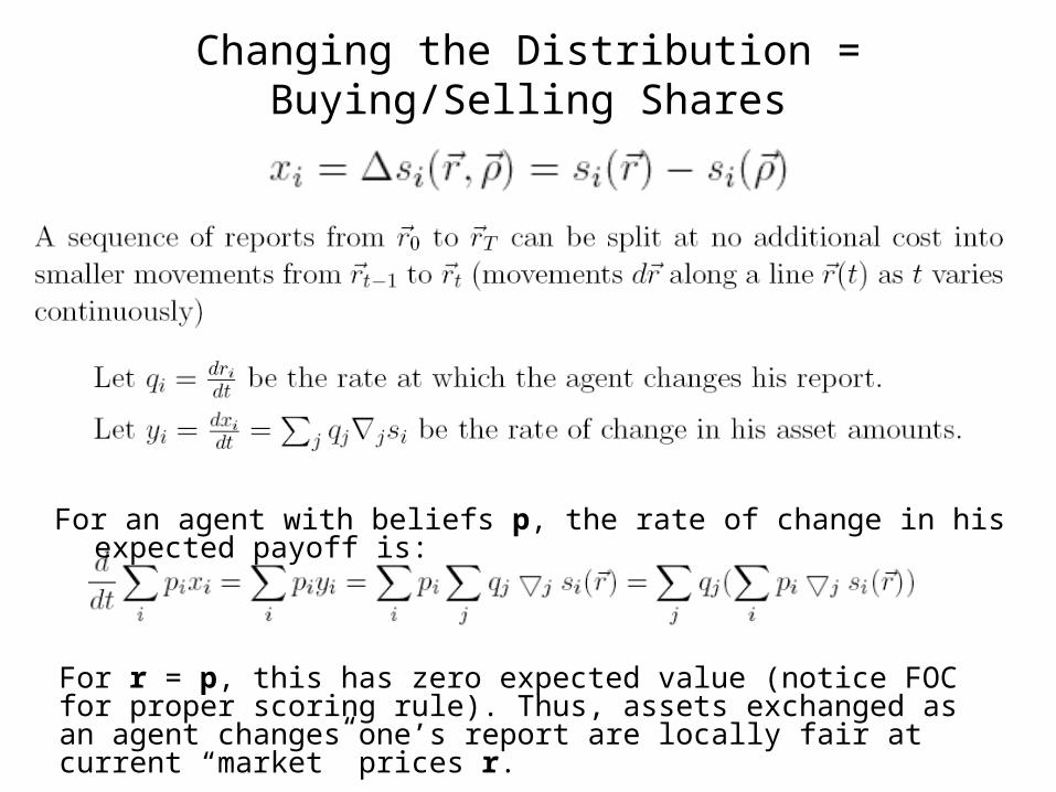
Changing the Distribution = Buying/Selling Shares
For an agent with beliefs p, the rate of change in his expected payoff is:
For r = p, this has zero expected value (notice FOC for proper scoring rule). Thus, assets exchanged as an agent changes one’s report are locally fair at current “market” prices r.

• So, we can think of a market scoring rule as a automated inventory-based market maker with: – Zero bid-ask spread for infinitesimal trades (which we
showed in the previous slide)– An internal state described by inventory of assets – Instantaneous price:
– Market maker will accept any fair bet s.t.
and any integral of infinitesimal trades.
Changing the Distribution = Buying/Selling Shares
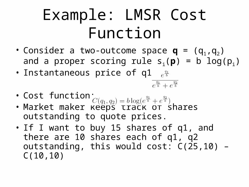
Example: LMSR Cost Function
• Consider a two-outcome space q = (q1,q2) and a proper scoring rule si(p) = b log(pi)
• Instantaneous price of q1:
• Cost function:• Market maker keeps track of shares outstanding
to quote prices.• If I want to buy 15 shares of q1, and there are 10
shares each of q1, q2 outstanding, this would cost: C(25,10) – C(10,10)

Modularity
• How well do MSR preserve conditional independence relations?
• Example: placing a bet on conditional event A given B should not change P(B) or P(C) for some event C unrelated to how A might depend on B
• Logarithmic rule bets on A given B preserve P(B), and for any event C, preserve P(C|AB), P(C|AcB), and P(C|Bc)
• Turns out LMSR is uniquely able to do this

Combinatorial Product Space
• Given N variables each with V outcomes, a single market scoring rule can make trades on any of the VN possible states, or any of the 2^(VN) possible events.
• Creating a data structure to explicitly store the probability of every such state is unfeasible for large values of N.
• Computational complexity of updating prices and assets is worse than polynomial in the worst case (NP-complete).

Ways to Deal with Large State Space
• Limit probability distribution– Example: Bayes Net – variables organized by a directed graph
where each variable has a set of parents. Probability of a state i can be written as:
which states that value of a variable in a state i can be computed based on the conditional dependencies with all parents.
– For a sparse network, this makes it easier to store the data as we need to keep track of fewer variables
Ways to Deal with Large State Space
– Problem: Supporting bets on conditional probabilities not specified in net or unconditional probabilities – harder to do unless you have “nearly” singly connected Bayes Net
– Using an approximation algorithm to calculate probabilities in a more complicated Bayes Nets runs risk of opening new arbitrage opportunities
• Use Multiple Market Makers– Example: Combine MSR that represents probabilities via a
general sparse Bayes net and a MSR that deals only with the unconditional probabilities
– Problem: Arbitrage opportunities across patrons, but the amount of loss is now bounded (since we can bound the loss for each rule).

Open Questions
• What’s the most effective way to set b, the liquidity constraint?– High b desirable for thin market, low b desirable for
thick market.
• How can we deal with large state space of allowing combinatorial outcomes?
• Does LMSR work as well as traditional prediction markets empirically?
• Do there exist circumstances where it makes strategic sense to bluff or hide information?