1

Lecture Slides by Dr. Muhammad Hanif Mian for Workshop on Recent Developments in Survey Sampling

(August 26-27, 06) AN ALTERNATIVE ESTIMATOR FOR Y Since repetition of the observation of a repeated unit in a sample selected with srswr does not provide additional information for estimatingY , the mean of the values of the distinct units in a sample of n units may be considered as an alternative estimator. That is, if

/ / /1 2, ,..., dy y y denote the values of the distinct units in a

simple random sample of n units selected with replacement ( )d n≤ , then the suggested alternative estimator is / /

1

1 d

iiy S y

d == (3.21)

This estimator is unbiased for Y and is more efficient than the sample mean y , namely,

1 1

1 1 ,n n

i i ii i

y y r yn n= =

′= =∑ ∑

where ir of is the number of repetitions of the i-th distinct

unit and 1

.d

iS ri n=

=

The variance of /y can be obtained by nothing that in this case two stages of randomization are involved: (i) d is a random variable taking values 1 to n with certain probabilities, and (ii) selection of the d distinct units from

2

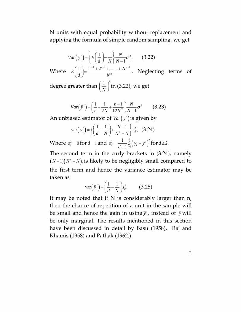
N units with equal probability without replacement and applying the formula of simple random sampling, we get

( )/ 21 1 ,1

NVar y Ed N N

σ⎧ ⎫⎛ ⎞= −⎨ ⎬⎜ ⎟ −⎝ ⎠⎩ ⎭ (3.22)

Where 1 1 11 1 2 .......n n n

n

NEd N

− − −+ + +⎛ ⎞ =⎜ ⎟⎝ ⎠

. Neglecting terms of

degree greater than 21

N⎛ ⎞⎜ ⎟⎝ ⎠

in (3.22), we get

( )/ 22

1 1 12 12 1

n NVar yn N N N

σ−⎛ ⎞= − +⎜ ⎟ −⎝ ⎠ (3.23)

An unbiased estimator of ( )/Var y is given by

( )/ 21 1 1var ,dn

Ny sd N N N

⎧ ⎫−⎛ ⎞= − +⎨ ⎬⎜ ⎟ −⎝ ⎠⎩ ⎭ (3.24)

Where 2 0ds = for 1d = and ( )22 / /

1

11

d

d iis S y y

d == −

−for 2.d ≥

The second term in the curly brackets in (3.24), namely ( )( )1 ,nN N N− − is likely to be negligibly small compared to the first term and hence the variance estimator may be taken as

( )/ 21 1var .dy sd N

⎛ ⎞= −⎜ ⎟⎝ ⎠

(3.25)

It may be noted that if N is considerably larger than n, then the chance of repetition of a unit in the sample will be small and hence the gain in using /y , instead of y will be only marginal. The results mentioned in this section have been discussed in detail by Basu (1958), Raj and Khamis (1958) and Pathak (1962.)

3

UNBIASED RATIO ESTIMATOR We have seen that under simple random sampling, classical (conventional) ratio estimator is biased. Lahiri (1951) suggested that classical ratio estimator can be made unbiased if the selection procedure is changed. Midzuno (1950) and Sen (1951) proved the same result. Lahiri suggested that the first unit was selected with probability proportional to the aggregate of the size (PPAS)

or with probability proportional to 1

N

ii

X=∑ , and the remaining n – 1 units

with equal probability and without replacement. Midzuno (1951) simplified this procedure as “the first unit is selected with probability proportional to Xi (measure of size), and the remaining (n – 1) units like Lahiri (1951)”. This idea was introduced by Ikeda (1950) – reported by Midzuno (1951). This sampling scheme has striking resemblance to the simple random sampling without replacement. In fact, it may be viewed as a generalization of the simple random sampling when extra information on the population is available. Let we have a population of N units. The probability that ith unit is first one to be selected and subsequent (n – 1) units with equal probability and without replacement is

1

111

iN

ii

xNXn=

−⎛ ⎞⎜ ⎟−⎝ ⎠

∑ .

The probability that jth unit is first one to be selected and subsequent (n – 1) draws with equal probability and without replacement

1

111

jN

ii

xNXn=

−⎛ ⎞⎜ ⎟−⎝ ⎠

∑,

and so on the probability P(s) for the two selections are therefore

1

1( )11

i jN

ii

x xP s

NXn=

+=

−⎛ ⎞⎜ ⎟−⎝ ⎠

∑.

Since there are n such selection therefore the probability of the selection of the sample will be

4

1 1( )11

n

ii

xP s

NXn

==−⎡ ⎤

⎢ ⎥−⎣ ⎦

∑ . (6.6.1)

1xNXn

=⎛ ⎞⎜ ⎟⎝ ⎠

. (6.6.2)

The classical ratio estimator is

1

1

n

iin

ii

yy X

x

=

=

′′ =∑

∑ (6.1.3)

THEOREM (6.2): Classical ratio estimator is unbiased under Ikeda-Midzuno- Sen –Lahiri selection procedure with variance

2

11 2

1

1( )

1

n

ii

n

ii

yN

Var y X Yn x

−=

=

⎡ ⎤⎛ ⎞⎢ ⎥⎜ ⎟−⎛ ⎞ ⎝ ⎠⎢ ⎥′′ ′= Σ −⎜ ⎟ ⎢ ⎥−⎝ ⎠ ⎢ ⎥⎢ ⎥⎣ ⎦

∑

∑ (6.6.3)

/Σ is the sum over all possible samples. PROOF Taking the expectation of (6.1.3) we have

1

1

( ) ( )

n

iin

ii

yE y P s X

x

=

=

⎡ ⎤⎢ ⎥

′′ ′= Σ ⎢ ⎥⎢ ⎥⎢ ⎥⎣ ⎦

∑

∑,

where P(s) is the probability of the sample..Putting the value of P(s) from (6.6.1) we will have

5

( )E y′′ 1 1

1

111

n n

i ii in

ii

y xX

NXxn

= =

=

⎡ ⎤⎢ ⎥⎢ ⎥′= Σ⎢ ⎥−⎛ ⎞⎢ ⎥⎜ ⎟−⎢ ⎥⎝ ⎠⎣ ⎦

∑ ∑

∑

On simplification we get

( )E y′′ 1 1

11

n n

i ii i

y N yy Y

N N Nn

n n n

= =

⎡ ⎤ ⎡ ⎤⎢ ⎥ ⎢ ⎥ ′⎢ ⎥ ⎢ ⎥′ ′ ′= Σ = Σ = Σ =⎢ ⎥ ⎢ ⎥−⎛ ⎞ ⎛ ⎞ ⎛ ⎞⎢ ⎥ ⎢ ⎥⎜ ⎟ ⎜ ⎟ ⎜ ⎟−⎢ ⎥ ⎢ ⎥⎝ ⎠ ⎝ ⎠ ⎝ ⎠⎣ ⎦ ⎣ ⎦

∑ ∑ ◊ (6.6.4)

The variance expression of y′′ may be derived as;

[ ]22( ) ( )Var y E y Ey′′ ′′ ′′= −

Var( y′′ )

2

1 22

1

( )

n

ii

n

ii

yP s X Y

x

=

=

⎡ ⎤⎛ ⎞⎢ ⎥⎜ ⎟⎝ ⎠⎢ ⎥′= Σ −⎢ ⎥⎛ ⎞⎢ ⎥⎜ ⎟⎢ ⎥⎝ ⎠⎣ ⎦

∑

∑

Substituting the value of P(s) from (6.6.1)

2

11 2

1

1( )

1

n

ii

n

ii

yN

Var y X Yn x

−=

=

⎡ ⎤⎛ ⎞⎢ ⎥⎜ ⎟−⎛ ⎞ ⎝ ⎠⎢ ⎥′′ ′= Σ −⎜ ⎟ ⎢ ⎥−⎝ ⎠ ⎢ ⎥⎢ ⎥⎣ ⎦

∑

∑.◊ (6.6.3)

Note that the ( ) 0 ii i i

i

XVar y if y x YX

⎛ ⎞′′ = ∝ =⎜ ⎟⎜ ⎟

⎝ ⎠∑. This is very strong

property and will be referred to as Ratio Estimator Property. THEOREM ( 6.3) The mean of ratio estimator is an unbiased with variance

1 2

2( )N yVar y X Yn x

−⎛ ⎞ ⎡ ⎤′′ ′= Σ −⎜ ⎟ ⎢ ⎥

⎣ ⎦⎝ ⎠ (6.6.5)

PROOF Taking the expectation of (6.1.4) we get

6

( ) yE y XEx

⎡ ⎤′′ = ⎢ ⎥⎣ ⎦ ( )y P s X

x⎡ ⎤′= Σ ⎢ ⎥⎣ ⎦

Using (6.6.2) we have

1( ) y xE y XNx Xn

⎡ ⎤⎢ ⎥⎢ ⎥′′ ′= Σ⎢ ⎥⎛ ⎞⎢ ⎥⎜ ⎟⎢ ⎥⎝ ⎠⎣ ⎦

Nn

y YC⎡ ⎤′= Σ =⎢ ⎥⎣ ⎦

◊ (6.6.5)

Proceeding by the same way as before we can derive the variance expression of y ′′ , i.e.

1 2

2( )N yVar y X Yn x

−⎛ ⎞ ⎡ ⎤′′ ′= Σ −⎜ ⎟ ⎢ ⎥

⎣ ⎦⎝ ⎠ (6.6.6)

THEOREM (6.4) An unbiased estimator of )y(Var ′′ is

2

2

1 1 1

1ar( )( 1)

n n ni

i ji i j

y X N Xv y y y yNn x Nn n x= = =

−′′ ′′= − −−∑ ∑ ∑ (6.6.7)

2 2 2y

X N ny y sx Nn

−⎡ ⎤′′= − −⎢ ⎥⎣ ⎦ (6.6.8)

PROOF It may be proved that [ ar( )] ( )E v y Var y′′ ′′= . For this

2 2

1 1

( )n n

i i

i i

y yX XE P sNn x Nn x= =

′⎡ ⎤ ⎡ ⎤=⎢ ⎥ ⎢ ⎥

⎣ ⎦ ⎣ ⎦∑ ∑ ∑

= 2

/ 1iy X xNN x Xn

⎡ ⎤⎢ ⎥⎢ ⎥⎢ ⎥⎛ ⎞⎢ ⎥⎜ ⎟⎢ ⎥⎝ ⎠⎣ ⎦

∑ 2

1

1 N

ii

YN =

= ∑ (6.6.9)

and

1 1

1 1( 1) ( )( 1) ( 1)

n n

i j i ji j

j i

N x NE y y n n E y ynN n X n n N= =

≠

⎡ ⎤− −⎢ ⎥ = −⎢ ⎥− −

⎢ ⎥⎣ ⎦∑∑

7

1 1

21 1

1 1( 1)

N N

i ji j N N

j ii j

i jj i

YYN YY

N N N N

= =≠

= =≠

−= =

−

∑∑∑∑ (6.6.10)

Hence

2 2( ) ( )E y Y Var y′′ ′′= − = Similarly we can show that an unbiased estimator of population total will be

2 2 2ar( ) yN X N nv y y y s

x Nn−⎡ ⎤′′ ′′= − −⎢ ⎥⎣ ⎦

RATIO ESTIMATOR AS MODEL-UNBIASED Consider all estimators y′ of Y that are linear functions of sample values yi, that are of the form

1

,n

i ii

y c y=

′ = ∑ (6.8.1)

where the ic does not depend on syi′ though they may a function xi. The choice of the ic s′ restricted to those that give unbiased estimation of Y. The estimator with the smallest variance is called best linear unbiased estimator. The model is:

2 2 2

,( ) 0, ( , ) 0,

1( ) 12

i i i

i i j

i i i

y xwhere E Cov

and Var X γ

β εε ε ε

ε σ σ γ

⎫⎪= +⎪⎪= = ⎬⎪⎪= = ≤ ≤⎪⎭

(6.8.2)

where εi are independent of the xi and xi are > 0. The xi (i = 1, 2, …… N) are known. The model is the same that was employed by Cochran (1953), which appears to have been originated by H.F. Smith (1938). Useful references to this model are Cochran (1953, 63, 77), Brewer (1963b), Godambe and Joshi (1965), Hanif (1969) Foreman and Brewer (1971), Royall (1970). (1975),Brewer and Hanif(1983) Cassel, et al (1976), Isaki and Fuller (1982), Hansen, Madow and Tepping (1983), Samiuddin et al (1992)and many others.

8

Brewer (1963b) defined an unbiased ratio estimator under model (6.8.2). He used the concept of unbiased ness which was different from that given in randomization (design - based) theory. Royall (1970) also used this model. Brewer and Royall regarded an estimator y′ (estimated population total) is unbiased if ( ) ( )YEyE =′ in repeated selections of the finite population and sampled under the model. Under model (6.8.2) Brewer (1963b) proved that the classical ratio estimate was model – unbiased and is best linear unbiased estimator for any sample [random or not] selected solely according to the values of the Xi. This result hold goods if the following line conditions are satisfied; (i) The relation between estimated (yi) and benchmark (xi) is linear and

passes though the origin. (ii) The Var(yi) about this line is proportional to xi. THEOREM (6.6): Under the model (6.8.2) classical ratio estimator is unbiased with variance

1 22( )

N yVar y X Yn x

−⎛ ⎞ ⎡ ⎤′′ ′= Σ −⎜ ⎟ ⎢ ⎥

⎣ ⎦⎝ ⎠= X

xn)xnX( −λ

= (6.8.3)

PROOF: We know that

1

n

i ii

y c y=

′ = ∑ (8.6.4)

Using model (6.8.2) we have

[ ]1 1 1

n n n

i i i i i i ii i i

y c x c x cβ ε β ε= = =

′ = + = +∑ ∑ ∑

Since E(εi) = 0 we then have

1 1

( ) ( )n n

i i i ii i

E y c x c Eβ ε= =

′ = +∑ ∑1

n

i ii

c xβ=

= ∑ (6.8.5)

We also know that i i iY Xβ ε= + or X)Y(E β= (6.8.6) Now

1 1 1

[ ] ( ) ( )N N N

i i i i ii i i

E y Y c x c E X Eβ ε β ε= = =

′ − = + − −∑ ∑ ∑

9

1 1

0n n

i i i ii i

c x X If c x Xβ= =

⎡ ⎤= − = =⎢ ⎥⎣ ⎦∑ ∑ (6.8.7)

Therefore we say that /y is model unbiased if

1

n

i ii

c x X=

=∑ (6.8.8)

The variance expression of /y , i.e.

[ ]22( ) ( ) ( )Var y E y E y′ ′ ′= − (6.8.9)

2 2 2 2 2 2 2

1 1

( ) ( ) 2 ( )n n n

i i i i i i ii i

E y c x c E c x Eβ ε β ε= =

′ = + +∑ ∑ ∑

Using the condition of model we will have:

2( )E y′ 2 2 2 2

1 1

( )n n

i i i ii i

c x c Varβ ε= =

= +∑ ∑ (6.8.10)

Using (6.8.2), (6.8.5) and (6.8.9) in (6.8.9), we will have

( )2

1

( )n

i ii

Var y c Varλ ε=

′ = ∑ (6.8.11)

Let us for simplicity we assume ( )i iVar xε λ= then (6.8.11) will be:

2

1

( )n

i ii

Var y c xλ=

′ = ∑ (6.8.12)

We can minimize /( )Var y w.r.t. ci. For this the Lagrange’s multiplier will be

2

1 1

n n

i i i ii i

c x c x Xφ λ µ= =

⎡ ⎤= − −⎢ ⎥⎣ ⎦∑ ∑

Differentiating unconditionally with respect to ci, we get.

2 0i i ii

c x xaφ λ µ∂= − =

∂

or 2ic Cµλ

= = (constant)

We know from (6.8.7) that 1

n

i ii

c x X=

=∑

or

1

,n

i ii

Xc x X or c cn x=

= = =∑

10

Hence /

1

n

i ii

y c y=

=∑ 1

1

1

n

ini

i ni

ii

yX y X y

n x x

=

=

=

′′= = =∑

∑∑

The best linear unbiased estimator yy/ ′′= , which is a classical (conventional) ratio estimator. For the derivation of )y(Var ′′ we proceed as follows:

1 1 1

n n N

i i i i ii i i

y Y c x c Xβ ε β ε= = =

′′ − = + − −∑ ∑ ∑

Since 1

n

i ii

c x X=

=∑ and 1 1

n N

i i ii i

X Xc then y Yn x n x

ε ε= =

′′= − = −∑ ∑

Divide ∑=ε

N

1ii into sample and non-sample values we have

1 1

n N

i i ii i

X Xa then y Yn x n x

ε ε= =

′′= − = −∑ ∑

or 1 1

( ) 1n N n

i ii i

Xy Yn x

ε ε−

= =

⎛ ⎞′′ − = − −⎜ ⎟⎝ ⎠

∑ ∑

Squaring and taking the expectation

( ) ( ) ( ) ( )2

2 2 2

1 1

1n N n

i ii i

XE y Y Var y E Enx

ε ε−

= =

⎛ ⎞′′ ′′− = = − +⎜ ⎟⎝ ⎠

∑ ∑

( ) ( ) ( )2

1 1

1 var varn N n

i ii i

XVar ynx

ε ε−

= =

⎛ ⎞′′ = − +⎜ ⎟⎝ ⎠

∑ ∑

Substituting the value of Var(xi), we have:

( )

( )

2

1

2

1 1

2

1N n

ii

N n

i i ii i

X nxVar y xnx

X nx x X xnx

X nx nx X nxnx

λ λ

λ λ

λ λ

−

=

= =

−⎛ ⎞′′ = − +⎜ ⎟⎝ ⎠

− ⎡ ⎤⎛ ⎞= + −⎜ ⎟ ⎢ ⎥⎝ ⎠ ⎣ ⎦

−⎛ ⎞= + −⎜ ⎟⎝ ⎠

∑

∑ ∑ ∑

2

2

( )( ) ( )( )X nxVar y nx X nxn x

λ λ−′′ = + − ( )X nx X

n xλ −

= (6.8.3)

11

Using all these assumptions a model-unbiased estimator λλ ofˆ from the sample may be easily proved as

2

1

1 1ˆ ( )1

n

i ii i

y r xn x

λ=

= −− ∑ . (6.8.13)

Putting this value of λ̂ in (6.8.4) a model-unbiased variance estimator is

2

1

( ) 1 1( ) ( )1

n

i ii i

X nx XVar y y rxn x n x=

−′′ = −− ∑ (6.8.14)

This model based unbiased estimator is not only superior to /y but is the best of a whole class of estimators. For details see Brewer (1963b, 1979), Royall (1970), Royall and Herson (1973) and Samiuddin et.al. (1978). 6.9 COMPARISON y ′′ AND /y UNDER STOCHASTIC MODEL It is an established fact that the choice of a suitable sample plan is central to the design of a sample survey. Sample design can be regarded as comprising separate selection and estimation procedures, but the choices of these are so interdependent that they must be considered together for virtually all purposes. Some times the nature of the sample plan is determined by circumstances, but usually the designer is faced with a choice, and frequently it is obvious which of a number of possible plan will be most efficient in terms of minimum sample error for given cost( or vice versa). Standard sampling theory using imputed values for such quantities as the means, variances, and correlation coefficient of the (finite) population, or strata or clusters within it, can often indicate which design is most efficient. Sometimes, however, this is not so. A well-known example is the comparison between classical ratio estimation using unequal probabilities. To obtain a straight forwarded answer in this case, Cochran (1953) made use of a certain super population (6.8.2) which is intuitively attractive and appears to have some empirical basis. The purpose here is to compare classical ratio estimator and unbiased estimation method of estimation using equal probabilities and using large scale sample result which can be obtained using generalization of model. Comparison for probability proportional to size will be discussed in Chapter 7, 8 and 9. The stochastic model used here for the purpose of comparing efficiencies. 6.9.1. Unbiased Estimate for Population Total Based on Simple Random

Sampling THEOREM (6.7). Under linear stochastic model (6.8.2) ratio estimator will be more efficient than

unbiased estimator if 2 2 2

1

N

x ii

β σ σ′=

> ∑

PROOF

12

We know that:

1

n

ii

Ny yn =

′ = ∑

Putting the value of (6.8.2) we get

( )1 1 1

n n n

i i i ii i i

N Ny x xn n

β ε β ε= = =

⎡ ⎤′ = + = +⎢ ⎥⎣ ⎦∑ ∑ ∑

=1

n

ii

Nxn

β ε=

′ + ∑ (6.9.1)

Also [ ]1 1 1

N N N

i i i ii i i

Y Y X Xβ ε β ε= = =

= = + = +∑ ∑ ∑ (6.9.2)

or 1

N

ii

Y Xε β=

= −∑ (6.9.3)

( ) ( )2Var y E y Y′ ′= −

[ ]2E y X X Yβ β′= − + −

( ) ( ) 2E y X Y Xβ β′⎡ ⎤= − − −⎣ ⎦

( ) ( )2 2E y X E Y Xβ β′= − − − (6.9.4)

as cross product term is equal to ( )22E Y Xβ− Now on first term of (6.9.4) using (6.8.2) will be

( )2

2

1

n

M D M D ii

NE E y X E E x Xn

β β ε β=

⎡ ⎤′ ′− = + −⎢ ⎥⎣ ⎦∑

( )2

1

n

M D ii

NE E x Xn

β ε=

⎡ ⎤′= − +⎢ ⎥⎣ ⎦∑

2 2 2

1

N

x ii

Nn

β σ σ′=

= + ∑ (6.9.5)

Similarly

( )2

2

1

N

M i Mi

E E Y Xε β=

⎛ ⎞ = −⎜ ⎟⎝ ⎠∑

13

or ( )22

1

N

ii

E Y Xσ β=

= −∑ (6.9.6)

Using (6.9.5) and (6.9.6) in (6.9.4) we get:

( ) 2 2 2 2

1

N

y x ii

N nVar yn

σ β σ σ′ ′=

−′ = = + ∑ (6.9.7)

Ratio Estimator

yy Xx′

′′ =′

(6.1.3)

( )

1

n

i ii

N Xn X

x

β ε=

+=

′

∑

1

n

ii

Nxn Xx

β ε=

⎡ ⎤′ +⎢ ⎥⎣ ⎦=′

∑ (6.9.8)

Now ( ) [ ]2Var y E y Y′′ ′′= −

[ ]2E y X X Yβ β′′= − + −

( ) ( )2 2E y X E Y Xβ β⎡ ⎤′′= − − −⎣ ⎦ (6.9.9)

Now

[ ]

2

2 1

n

ii

M D M D

NxnE E y X E E X Xx

β εβ β=

⎡ ⎤′ +⎢ ⎥′′ − = −⎢ ⎥

′⎢ ⎥⎢ ⎥⎣ ⎦

∑

2

1

n

M D ii

N XE E X Xn x

β ε β=

⎡ ⎤= + −⎢ ⎥′⎣ ⎦∑

2

1

n

M D ii

N XE En x

ε=

⎡ ⎤= ⎢ ⎥′⎣ ⎦∑

22

21

N

ii

N Xn x

σ=

=′ ∑

2

1

N

ii

Nn

σ=

= ∑

(6.9.10) 2

1( )

N

ii

E Y Xβ σ=

− =∑

Therefore

14

( )Var y′′ = 2

1

N

ii

Nn

σ=

= ∑ - 2

1

N

iiσ

=∑

Comparing (6.9.7) and (6.9.11) we have:

( ) ( ) 2 2 2 2 2

1 1 1

N N N

x i i ii i i

N NVar y Var yn n

β σ σ σ σ′= = =

′ ′′− = + − −∑ ∑ ∑ -

2

1

N

iiσ

=∑

2 2xβ σ ′= So Ratio Estimator will always be more efficient if 2 2 2

1

N

x ii

β σ σ′=

= −∑ is

positive or Foreman and Brewer (1971) used the following model i i iY Xα β ε= + + With the same assumption given in (6.8.2) they compared various method of estimation and proved that ratio method of estimation is more efficient than unbiased estimation method provided | α | < | βX | .. SOME RECENT DEVELOPMENTS ON RATIO ESTIMATORS Recently two benchmark variables have been used to increase the efficiency. Some of them are given here 6.10 1 Modification of Classical Ratio Estimator – I Chand’s (1975) developed a chain ratio type estimator in the context of two phase sampling. It seems sensible to study the possibility of adapting it to the new situation although the force of its argument is somewhat lost in the single phase case. THREROM (6.8). An estimator suggested by Samiuddin and Hanif (2006) by using two auxiliary variables i.e, ratio cum ratio is

2X ZT yx z

= (6.10.1)

With Mean square error is

15

( ) 2 2 2 22 1 2 2 2y x z x y yx y z yz x z xzMSE T Y C C C C C C C C C⎡ ⎤= θ + + − ρ − ρ + ρ⎣ ⎦ (6.10.2)

The construction of this estimator is made multiplying Classical Ratio estimator

by Zz

.

PROOF Using the concept given in (6.2.23) we get

( )2 1 1x zy

e eT Y Y e Y

X Z⎡ ⎤⎛ ⎞⎛ ⎞− = + − − −⎢ ⎥⎜ ⎟⎜ ⎟

⎝ ⎠⎝ ⎠⎣ ⎦ (6.10.3)

Ignoring send and higher order terms we get

2 y x zY YT Y e e eX Z

− − −; (6.10.4)

The mean square error 3T will be

( )22E T Y− =2

X Zy Yx z

⎛ ⎞= −⎜ ⎟⎝ ⎠

(6.10.5)

Using (6.10.4) in (6.10.5) we get

( )

22

2

2 2 22 2 2

2 2 2 2 2

y x z

y x z y x y z x z

Y YE T Y E e e eX Z

Y Y Y Y YE e e e e e e e e eX Z XZX Z

⎛ ⎞− − −⎜ ⎟

⎝ ⎠⎡ ⎤

+ + − − +⎢ ⎥⎣ ⎦

;

;

Applying expectation we get

( )2 2

2 2 2 2 2 22 1 2 2

2

2

2 2

y x z x y xy

y z yz x z xz

Y Y YMSE T Y C C X C Z Y XC CXX Z

Y YY ZC C XZC CZ X Z

⎡θ + + − ρ⎢⎣

⎤− ρ + ρ ⎥

⎦

;

On simplification we get ( ) 2 2 2 2

2 1 2 2 2y x z x y yx y z yz x z xzMSE T Y C C C C C C C C C⎡ ⎤= θ + + − ρ − ρ + ρ⎣ ⎦ (6.10.2) 2 2 2 2 2

2 1 1( ) [ 2 ] [ 2 2 ]y x xy x y z y z yz x z xzMSE T Y C C C C Y C C C C Cθ ρ θ ρ ρ= + − + − +

2 2

2 1 1( ) ( ) [ 2 2 ]z y z yz x z xzMSE T MSE T Y C C C C Cθ ρ ρ= + − + (6.10.2)

6.10.2 Revised Ratio Estimator( An Estimator with suitable “a” involving two auxiliary variables)

16

THEOREM (6.9). A possible estimator with the involvement of suitable “a” and with two auxiliary variable suggested by Samiuddin and Hanif (2006) is

( )3 1X ZT a y a yx z

⎛ ⎞ ⎛ ⎞= + −⎜ ⎟ ⎜ ⎟

⎝ ⎠ ⎝ ⎠ , (6.10.6)

with mean square error

( ) ( )222 2 2

3 1 2 222

x y xy y z yz x z xz zy z yz y z

x z x z xz

C C C C C C CMSE T Y C C C C

C C C C

⎡ ⎤ρ − ρ − ρ +⎛ ⎞ ⎢ ⎥=θ + − ρ −⎜ ⎟ ⎢ ⎥⎜ ⎟ + − ρ⎝ ⎠ ⎢ ⎥⎣ ⎦

(6.10.7) PROOF Using the concept given in (6.2.23)

( )

1 1+ ⎛ ⎞ ⎛ ⎞

= + −⎜ ⎟ ⎜ ⎟⎜ ⎟+ ⎝ ⎠⎝ ⎠;

y y x

x

Y e e eyX X Y

x X e Y X

Expanding and ignoring second and higher order terms we get

y Xx

1 .... ....⎡ ⎤

= + − + = + − +⎢ ⎥⎣ ⎦

y xy x

e e YY Y e eY X X (6.10.8).

Similarly

( )1 1y y z

z

Y e e ey Z Z Yz Z e Y Z

+ ⎛ ⎞⎛ ⎞= + −⎜ ⎟⎜ ⎟+ ⎝ ⎠⎝ ⎠;

1 .... ....⎡ ⎤

= + − + = + − +⎢ ⎥⎣ ⎦

y zy z

e e YY Y e eY Z Z (6.10.9)

Using (6.10.8) and (6.10.9) 3T will be

3T ( ) ( ) ( )1y yx z

X ZY e Y eX e Z e

α α⎧ ⎫ ⎧ ⎫⎪ ⎪ ⎪ ⎪= + + − +⎨ ⎬ ⎨ ⎬

+ +⎪ ⎪⎪ ⎪ ⎩ ⎭⎩ ⎭

( ) ( ) ( )1 1 1x zy y

e eY e Y eX Z

α α⎧ ⎫⎛ ⎞ ⎛ ⎞⎪ ⎪+ − + − + −⎜ ⎟ ⎜ ⎟⎨ ⎬ ⎜ ⎟⎜ ⎟⎪ ⎪ ⎝ ⎠⎝ ⎠⎩ ⎭

( )1y x zY YY e e eX Z

α α+ − − −

The mean square error will be

17

2

3( ) y z x zY Y YMSE T e e e eZ X Z

α⎡ ⎤⎛ ⎞

= − − −⎢ ⎥⎜ ⎟⎝ ⎠⎣ ⎦

This may be written as

( ) ( )2

3 1X ZMSE T E a y Y a y Yx z

⎡ ⎤⎛ ⎞ ⎛ ⎞− + − −⎢ ⎥⎜ ⎟ ⎜ ⎟

⎝ ⎠ ⎝ ⎠⎣ ⎦; (6.10.10)

2

⎡ ⎤= − + − − +⎢ ⎥

⎣ ⎦y x y z y z

Y Y YE ae a e e e ae a eX Z Z

2

⎡ ⎤= − − +⎢ ⎥

⎣ ⎦y x z z

Y Y YE e a e e a eX Z Z

2

⎡ ⎤⎛ ⎞= − − −⎢ ⎥⎜ ⎟

⎝ ⎠⎣ ⎦y z x z

Y Y YE e e a e eZ X Z

(6.10.11)

In order to get the optimum value of “a” we first find partial differentiating of (6.10.11) w.r.t “a” and then equating to zero.

2

0⎡ ⎤⎡ ⎤⎛ ⎞ ⎛ ⎞ ⎛ ⎞⎢ ⎥− − − − =⎢ ⎥⎜ ⎟ ⎜ ⎟ ⎜ ⎟⎢ ⎥⎝ ⎠ ⎝ ⎠ ⎝ ⎠⎣ ⎦ ⎣ ⎦

y z x z x zY Y Y Y YE e e e e Ea e eZ X Z X Z

Therefore optimum value of “a” is

2

⎡ ⎤⎛ ⎞ ⎛ ⎞− −⎢ ⎥⎜ ⎟ ⎜ ⎟

⎝ ⎠ ⎝ ⎠⎣ ⎦=⎛ ⎞

−⎜ ⎟⎝ ⎠

y z x z

x z

Y Y YE e e e eZ X Z

aY YE e eX X

2 22

2

2 2 22 2

2 22

⎡ ⎤− − +⎢ ⎥

⎣ ⎦=⎡ ⎤

+ −⎢ ⎥⎣ ⎦

y x y z z x z

x z x z

Y Y Y YE e e e e e e eX Z ZX Z

Y Y YE e e e eXZX Z

2 2 2 2 2

2 2 2 2 22

⎡ ⎤θ ρ − ρ − ρ +⎣ ⎦=⎡ ⎤θ + − ρ⎣ ⎦

y x xy y z yz x z xz z

x z x z xz

Y C C Y C C Y C C Y C

Y C Y C Y C C

18

2 2

2 2 2 2

⎡ ⎤θ ρ − ρ − ρ +⎣ ⎦=⎡ ⎤θ + − ρ⎣ ⎦

y x xy y z yz x z xz z

x z x z xz

Y C C C C C C C

Y C C C C

2

2 2 2

ρ − ρ − ρ +=

+ − ρy x xy y z yz x z xz z

x z x z xz

C C C C C C Ca

C C C C (6.10.12)

Taking the square of (6.10.11)

2 2

2 2⎛ ⎞ ⎛ ⎞ ⎛ ⎞ ⎛ ⎞

= − + − − − −⎜ ⎟ ⎜ ⎟ ⎜ ⎟ ⎜ ⎟⎝ ⎠ ⎝ ⎠ ⎝ ⎠ ⎝ ⎠

y z x z y z x zY Y Y Y Y YE e e a E e e aE e e e eZ X Z Z X Z

2 2 2

2 2 2 2 22 2 2

2 2⎡ ⎤ ⎡ ⎤

= + − + + −⎢ ⎥ ⎢ ⎥⎣ ⎦ ⎣ ⎦

y z y z x z x zY Y Y Y Y YE e e e e a E e e e e

X X ZX X Z

2 2

22

2⎡ ⎤

− − − +⎢ ⎥⎣ ⎦

y x y z z x zY Y Y YaE e e e e e e eX Z Z X Z

Applying expectation the mean square error will be

( ) 2 2 2 2 2 2

3

2

2 2

2

y z yz y z x z x z xz

y x yx y z yz x z xz z

MST T Y C C C C a C C C C

a C C C C C C C

⎡ ⎤ ⎡ ⎤= θ + − ρ + + − ρ⎣ ⎦ ⎣ ⎦⎡ ⎤− ρ − ρ − ρ +⎣ ⎦

(6.10.13) Putting the value of “a” from (6.10.12) in (6.10.13) and on simplification we

( ) ( ) ( )222 2 2

3 2 222

x y xy y z yz x z xz zy z yz y z

x z x z xz

C C C C C C CMSE T Y C C C C

C C C C

⎡ ⎤ρ − ρ − ρ +⎢ ⎥=θ + − ρ −⎢ ⎥+ − ρ⎢ ⎥⎣ ⎦

(6.10.7

Since 0 and 1α α= = are special cases of 5T therefore we conclude that

( )5MSE T XMSE yx

⎛ ⎞≤ ⎜ ⎟

⎝ ⎠ and

ZMSE yz

⎛ ⎞⎜ ⎟⎝ ⎠

. In 5T , α will have to be replaced

by its sample estimate . SAMPLING WITH PROBABILITIES PROPORTIONAL

TO SIZE (WITH REPLACEMENT)

19

7.1. INTRODUCTION. In previous chapters equal probability sampling selection procedure and estimation methods have been discussed. In this and subsequent chapters those selection procedures will be considered in which probability of selection varies from unit to unit (unequal probability) in the population. In equal probability sampling, selection does not depend how large or small that unit is but in probability proportionate (proportional) to size sampling these considerations are made. The probabilities must be known for all units of the population. The general theory of unequal probabilities in sampling was perhaps first presented by Hansen and Hurwitz (1943). They demonstrated, however, that use of unequal selection probabilities within a stratum frequently made far more efficient estimator of total than did equal probability selection provided measure

of size ( iZ i.e. 1

N

ii

Z Z=

=∑ ) is sufficiently correlated with estimand,( variable

under study) Yi. A method of selection in which the units are selected with probability proportionate (proportional) to given measure of size, related to the characteristic under study is called unequal probability sampling or the probability proportional to size sampling, commonly known as PPS or πPS sampling. 7.2. SAMPLING WITH UNEQUAL PROBABILITIES WITH

REPLACEMENT [PPS SAMPLING]. The use of unequal probabilities in sampling was first suggested by Hansen and Hurwitz (1943). Prior to that date there had been substantial developments in sampling theory and practice, but all these had been based on the assumption that probabilities of selection within each stratum would be equal. They proposed a two stage sampling scheme (will be discussed in Chapter 11). The first stage selection took place in independent draws. At each draw, a single first-stage unit is selected with probabilities proportional to a measure of size, the number of second-stage sampling units within each first-stage units. At the second-stage, the same number of second stage-units is selected from each sampled first-stage unit. Because it is possible for the same first-stage unit to be selected more than once therefore, this type of unequal probability sampling is generally known as sampling with replacement. Since, however, the independence of the draws is not necessary condition for the units to have a non-zero probability of being selected more than once, another name first suggested by Hartley and Rao (1962) is

20

multinomial sampling, a term justified by the multinomial distribution of the number of units in the sample. Unequal probability can however be used in single stage design. This scheme compared favorably with other two –stage sampling schemes; these used equal probabilities of selection at the first stage, and then took either a fixed number or a constant proportion of sub-sampling units from each selected first stage unit. This selection procedure is explained as: A list of 523 villages of Multan district along with population of males and females is given in Appendix-I. In order to understand the selection procedure of probability proportional to size sampling, 5% sample has been selected from this population. In order to select a sample we cumulate the measure of sizes (area) under this selection procedure, 26(5% of total villages) random numbers are selected from 001 to 956204. These random numbers along with the serial number of villages, total population and initial probabilities of selection are given(data is given on next page). If any unit is selected more than once it should be included in the sample 7.3 EXPECTATION. If the ith unit is selected from a population of N units with probability

1/

N

i i ii

P Z Z=

= ∑ , than an unbiased estimator, HH ppsy or y′ ′ of population total Y

as suggested by Hansen and Hurwitz (1943) is:

1

1 ,n

iHH PPS

i i

yy yn p=

′ ′= = ∑ (7.3.1)

where HH denotes the Hansen and Hurwitz, and pps denotes probability proportional to size. THEOREM (7.1)

A sample of size n is drawn from a population of N units with probability proportional to size and with replacement HHy′ is an unbiased estimator of population total, Y.

PROOF We know that

21

1

1 ,n

iHH

i i

yyn p=

′ = ∑ (7.3.1)

Taking the expectation

1 1

1( ) ( ) ( )n N

i i iHH i

i ii i i

y y YE y E E P Yn p p P= =

′ = = = =∑ ∑ ◊

Therefore HHy′ is an unbiased estimator of population total Y.

Random number Sr. number of villages

Total population Probability of Selection

859677 483 7346 .005946 74835 50 9231 .006511 491741 275 3713 .001335 285996 131 2310 .001337 252541 108 7261 .006127 287850 133 10425 .00353 847258 478 6978 .006409 410596 221 399 .000316 674344 397 737 .002414 727666 423 3203 .001396 920794 508 4039 .002813 291874 135 5439 .000906 742201 434 1373 .000885 37860 33 8074 .006968 750855 437 3416 .00166 91613 54 5841 .003874 757074 441 1316 .002297 213334 92 6475 .004451 656265 385 1261 .002064 843800 478 6975 .006409 464793 258 2513 .002781 598479 360 3039 .001128 314161 153 322 .000697 820668 472 13056 .00613 18504 19 593 .000998 32315 28 2515 .001936

7.4. VARIANCE AND UNBIASED VARIANCE ESTIMATOR

22

THEOREM (7.2)

A sample of size n is drawn from a population of N units with probability proportional to size and with replacement, the variance of HHy′ is

22

1

1( )N

iHH

i i

YVar y Yn P=

⎛ ⎞′ = −⎜ ⎟

⎝ ⎠∑ (7.4.1)

PROOF.

We know that 2 2( ) ( )HH HHVar y E y Y′ ′= −

Substituting the value, HHy′ from (7.3.1), we have

2

2

1

1( )n

iHH

i i

yVar y E Yn p=

⎛ ⎞′ = −⎜ ⎟

⎝ ⎠∑

22

2 21 1 1

1 i

i

n n ni j

i i j i jj i

y y yE E Y

n p p p= = =≠

⎡ ⎤⎛ ⎞⎛ ⎞⎢ ⎥⎜ ⎟= + −⎜ ⎟⎢ ⎥⎜ ⎟⎜ ⎟ ⎜ ⎟⎝ ⎠⎢ ⎥⎝ ⎠⎣ ⎦

∑ ∑∑

22

2 21 1 1

1 ( 1)i

i

N N Ni j

i iji i j i j

j i

Y YYn P n n P Y

n P PP= = =≠

⎡ ⎤⎢ ⎥= + − −⎢ ⎥⎢ ⎥⎣ ⎦∑ ∑∑ .

Since the selection of population units are independent; therefore Pij = PiPj, substituting the value of pij:

22 2 2

1 1 1

1( ) ( 1) ( )iN N N

HH i ii i ii

YVar y n Y Y Y

n P= = =

⎡ ⎤⎛ ⎞′ = + − − −⎢ ⎥⎜ ⎟⎝ ⎠⎢ ⎥⎣ ⎦

∑ ∑ ∑ .

On simplification we get:

22

1

1( ) iN

HHi i

YVar y Y

n P=

⎡ ⎤′ = −⎢ ⎥

⎢ ⎥⎣ ⎦∑ ◊

This expression may alternatively be written as

23

2

1

1( )N

iHH i

i i

YVar y P Yn P=

⎡ ⎤′ = −⎢ ⎥

⎣ ⎦∑ . (7.4.2)

2

1 1

12

N Nji

i ji j i j

YYPPn P P= =

⎡ ⎤= −⎢ ⎥

⎢ ⎥⎣ ⎦∑∑ (7.4.3)

2

1

1 1 ( )N

i ii i

Y P Yn P=

= −∑ . (7.4.4)

7.4.1 An Alternative proof( using Indicator Variable) Let ai is defined as the number of times that the ith unit of the population to be in the sample (Chapter 2), then the joint distribution of ai is

1 2!1 2

1 2! ! !Naa a

NN

n P P Pa a a

KK

(7.4.5)

Then

( ) ; ( ) (1 ); ( , )i i i i i i j i jE a nP Var a nP P Cov a a nPP= = − = − (7.4.6) An unbiased estimator of population total will be

1

1 Ni

HH ii i

Yy an P=

′ = ∑ (7.4.7)

The unbiased ness can be proved easily as:- Taking the expectation of (7.4.7) and putting E(ai) = nPi from (7.4.6) we get

1 1

1 1( ) ( )N N

i iHH i i

i ii i

Y YE y E a nP Yn P n P= =

′ = = =∑ ∑

24

The variance of HHy′ may be written (see chapter 2) as:

2

2 21 1 1

1( ) ( ) ( , )N N N

ji iHH i i j

i i ji i jj i

YY YVar y Var a Cov a an P P P= = =

≠

⎡ ⎤⎢ ⎥′ = +⎢ ⎥⎢ ⎥⎣ ⎦∑ ∑ ∑ (7.4.8)

Putting the values of ( )iVar a and ( , )i jCov a a from (7.4.6) in (7.4.8) and on simplification we get (7.4.1).

It follows that, if 1

/N

i i ii

P Y Y=

= ∑ the variance is zero. In practice, this ideal

situation can of course not be realized as the probabilities cannot be chosen proportional to Yi, which still has to be observed. But this situation can be approximated if it is possible to choose Pi proportional to some measures of size Zi, which is known for all units in the population and which may be assumed approximately proportional to iY . The iZ will then be called the size of the ith unit and least possible variance may be obtained by choosing the probabilities proportional to the sizes.

An analogous expression for the covariance of HHy′ and HHx′ in the case of sampling with replacement and with probabilities proportional to size may be written in a straight far warded manner, i.e.

1

1( , )N

i ii

i i i

Y XCov y x P Y Xn P P=

⎛ ⎞ ⎛ ⎞′ ′ = − −⎜ ⎟ ⎜ ⎟

⎝ ⎠ ⎝ ⎠∑ . (7.4.9)

7.4.1. Unbiased Variance Estimator THEOREM (7.3) A sample of size n is drawn from a population of N units with probability

proportional to size and with replacement then an unbiased variance

estimator of (7.4.1) is:

2

1

1var( )( 1)

ni

HH HHi i

yy yn n p=

⎛ ⎞′ ′= −⎜ ⎟− ⎝ ⎠

∑ . (7.4.10)

25

PROOF. Taking expectation of (7.4.10)

[ ]2

1

1var( )( 1)

ni

HH HHi i

yE y E yn n p=

⎡ ⎤⎛ ⎞′ ′⎢ ⎥= −⎜ ⎟−⎢ ⎥⎝ ⎠⎣ ⎦

∑ ,

Now

( )2 2

2

1 1

n ni i

HH HHi ii i

y yy Y n E y Yp p= =

⎛ ⎞ ⎛ ⎞′ ′− = − − −⎜ ⎟ ⎜ ⎟

⎝ ⎠ ⎝ ⎠∑ ∑ .

Taking the expectation of the above equation

( )2HH

n

1i

2

i

in

1i

2

HHi

i YyEnYpy

Eypy

E −′−⎥⎥⎦

⎤

⎢⎢⎣

⎡∑ ⎟⎟

⎠

⎞⎜⎜⎝

⎛−=

⎥⎥⎦

⎤

⎢⎢⎣

⎡∑ ⎟⎟

⎠

⎞⎜⎜⎝

⎛′−

==

( ) ( ) ( )

2

1

22

1

( )

1 var 1 var

Ni

i HHi i

Ni

i HH HHi i

Yn P Y n Var yP

Yn P Y n y n n yn P

=

=

⎛ ⎞′= − −⎜ ⎟

⎝ ⎠

⎛ ⎞′ ′= − − = −⎜ ⎟

⎝ ⎠

∑

∑

Using (7.4.2) we get 2

1

ni

HHi i

yE yp=

⎡ ⎤⎛ ⎞′⎢ ⎥−⎜ ⎟

⎢ ⎥⎝ ⎠⎣ ⎦∑ ( 1) ( )HHn n Var y′= − .

Using this result in (7.4.10), we get

[ ]var( ) ( )HH HHE y Var y′ ′=

(7.4.10) may be written as

( )

2

21 1

1var( )2 1

n nji

HHi j i j

yyyn n p p= =

⎛ ⎞′ = −⎜ ⎟⎜ ⎟− ⎝ ⎠

∑∑ . (7.4.11)

For calculation purpose alternative form of (7.4.10) is

2'2

21

1var( )( 1

ni

HH PPSi i

yy n yn n p=

⎡ ⎤′ = −⎢ ⎥− ⎣ ⎦

∑ . (7.4.12)

26

An unbiased covariance expression may be written analogous to (7.4.9) as

1

1( , ) ( )( )( 1)

nii

HH HHi i i

xyCov y x y xn n p p=

′ ′ ′ ′= − −− ∑ . (7.4.13)

Though this scheme is based on with replacement process but for the following reasons, it is preferred to be used in large scale sample surveys;

(i) selection of the sample is simple,

(ii) can be used for any finite predetermined number of units in the sample,

(iii) an unbiased variance estimator is simple, and

(iv) it is also comparatively easy to obtain unbiased variance estimator of total in multistage designs.

This selection procedure may be more efficient than simple random

sampling if the measure of size is approximately proportional to estimated i.e. Yi and Zi are linearly related and regression line passing through the origin.

EXAMPLE (7.2)

Select a sample of 26 villages using probability proportional to size and with replacement selection procedure form the data given in Appendix-I. Estimate the total number of person in 523 villages and compare this result with actual number of population given in 523 villages. Estimate )y(Var PPS′ and calculate standard error of this estimate. Solution:

Sr. No. iy ip i

i

yp

2

i

i

y yp

⎛ ⎞′−⎜ ⎟

⎝ ⎠

2

2i

i

yp

2i

i

yp

1 7346 0.005946 1235452.405 137886694865.41 1.52634E+12 9075633367 2 9231 0.006511 1417754.569 35731892260.18 2.01003E+12 13087292428 3 3713 0.001335 2781273.408 1379426820568.15 7.73548E+12 10326868165 4 2310 0.001337 1727748.691 14632605885.20 2.98512E+12 3991099476 5 7261 0.006127 1185082.422 177831700028.54 1.40442E+12 8604883467 6 10425 0.00353 2953257.79 1812993331051.22 8.72173E+12 30787712465 7 6978 0.006409 1088781.401 268326052675.04 1.18544E+12 7597516617 8 399 0.000316 1262658.228 118422122062.40 1.59431E+12 503800632.9

27

9 737 0.002414 305302.403 1693852740901.42 93209557065 225007870.8 10 3203 0.001396 2294412.607 472833951008.72 5.26433E+12 7349003582 11 4039 0.002813 1435833.63 29223818023.56 2.06162E+12 5799332030 12 5439 0.000906 6003311.258 19329457362517.20 3.60397E+13 32652009934 13 1373 0.000885 1551412.429 3065942449.29 2.40688E+12 2130089266 14 8074 0.006968 1158725.603 200755773987.28 1.34265E+12 9355550517 15 3416 0.00166 2057831.325 203444246707.55 4.23467E+12 7029551807 16 5841 0.003874 1507743.934 9808812374.83 2.27329E+12 8806732318

28

Sr. No. iy ip i

i

yp

2

i

i

y yp

⎛ ⎞′−⎜ ⎟

⎝ ⎠

2

2i

i

yp

2i

i

yp

17 1316 0.002297 572921.202 1068871009157.62 3.28239E+11 753964301.3 18 6475 0.004451 1454729.274 23120451813.51 2.11624E+12 9419372051 19 1261 0.002064 610949.612 991684897660.22 3.73259E+11 770407461.2 20 6975 0.006409 1088313.309 268811216688.66 1.18443E+12 7590985333 21 2513 0.002781 903631.787 494422166072.03 8.1655E+11 2270826681 22 3039 0.001128 2694148.936 1182363847314.18 7.25844E+12 8187518617 23 322 0.000697 461979.910 1310574981674.20 2.13425E+11 148757532.3 24 13056 0.00613 2129853.181 273602014185.76 4.53627E+12 27807363132 25 593 0.000998 594188.377 1025348645657.47 3.5306E+11 352353707.4 26 2515 0.001936 1299070.248 94687373182.90 1.68758E+12 3267161674

117850 0.081318 41776367.9425 32621180470772.50 99746754265786.8 217890794431.5760

(i) Estimated Total ∑=

=′=n

1i i

iPPS p

yn1y

41776367.9425 160678326

= =

whereas the actual/total for 523 villages is 1797841.

(ii) ∑−

⎟⎟⎠

⎞⎜⎜⎝

⎛′−

−=′

n

iPPS

i

iPPS y

py

nnyVar

1

2

)1(1)(

350186431492625

50.07723262118047=

×=

29

(iii) 2834.224023)(. =′PPSyES

(iv) ( ). 1606783 2 224023.2834PPSC L y′ = ± × This may also be calculated as:

( )PPSvar y′ = ( )

22

2

11

ipps

i

y nyn n p

⎡ ⎤′−⎢ ⎥− ⎣ ⎦

∑

= ( )[ ]2382.16067832680.578699746754262625

1−

×

= 50186431493 7.4.2. Comparison of Simple Random Sampling with Replacement and Probability Proportional to Size with Replacement We know that

22

1

1( )N

iHH

i i

YVar y Yn P=

⎛ ⎞′ = −⎜ ⎟

⎝ ⎠∑ (7.4.1)

If Pi =1/N then (7.4.1) becomes

22 2 2

1

1( )N N

ran i ii

N YVar y N Y Y Yn n N=

⎛ ⎞⎛ ⎞′ = − = −⎜ ⎟⎜ ⎟⎝ ⎠ ⎝ ⎠∑ ∑ (7.4.14)

which is a variance expression for simple random sampling with replacement.

Putting Pi = Zi/Z in (7.4.1) and subtracting from (7.4.14), we obtain

2

1( ) ( ) 1

N

ran HH ii i

N ZVar y Var y Yn Z=

⎛ ⎞′ ′− = −⎜ ⎟

⎝ ⎠∑ , (7.4.15)

where 1

/N

ii

Z Z N=

= ∑ .

Probability Proportional to size (PPS) sampling with replacement will be more efficient than simple random sampling provided.

2

1

( ) 0N

ii

i i

YZ ZZ=

− >∑ (7.4.16)

i.e. If Zi and 2 /i iY Z are positively correlated.

However, it was noted by Raj (1954) that estimator based on PPS sampling with replacement turns out to be inefficient compared to unbiased estimate based on simple random sampling with replacement if the regression line Yi on Zi is far from the origin.

30

7.4.3Comparison of )y(Var ran′ and )y(Var HH′ Using a Linear Stochastic Model We have already shown in (7.4.2) thatt

2

1( ) ( ) 1

N

ran HH ii i

N ZVar y Var y Yn Z=

⎛ ⎞′ ′− = −⎜ ⎟

⎝ ⎠∑ (7.4.15)

( )2

1

Ni

ii i

YN Z Zn Z=

= −∑ (7.4.17)

For the purpose of comparison, let us take the linear model as defined in (6.8.2) the Chapter 6, i.e. Assuming that the finite population Y1, Y2, …., YN is a random sample from an infinite super-population in which i i iY Zβ ε= +

* *

2 2 2 2 2

( ) 0, ( ) 0,1( ) , 12

i i j

i i i i

where E E

E and Z whereγ

ε ε ε

ε σ σ σ γ

⎫= =⎪⎬

= = ≤ ≤ ⎪⎭

(6.8.2)

Substituting the value of Yi from the model in (7.4.17), we have

( )2 2 2

1

22

1

( ) ( ) 2

2

N

ran HH i i i ii

Ni

i ii i

NVar y Var y Z Zn

Z ZZ

β ε β ε

εβ βε

=

=

⎡′ ′− = + + +⎢⎣⎤⎛ ⎞

− + + ⎥⎜ ⎟⎥⎝ ⎠⎦

∑

∑

Using the condition of the model

2 2 2

1 1

N N

i ii i

N Zn

β ε= =

⎛ ⎞= +⎜ ⎟⎝ ⎠

∑ ∑2

2

1 1

N Ni

ii i i

Z Z ZZεβ

= =

⎡ ⎤⎛ ⎞− +⎢ ⎥⎜ ⎟⎢ ⎥⎝ ⎠⎣ ⎦

∑ ∑

2

212 2 2 2 21

1 1 1

N N

i iN N Ni i i

i ii i i i

Z ZZN Z Z

n N N Z

γγβ σ σ= =

= = =

⎡ ⎤⎛ ⎞⎛ ⎞⎢ ⎥⎜ ⎟⎜ ⎟⎝ ⎠⎢ ⎥⎜ ⎟= − + −⎢ ⎥⎜ ⎟

⎢ ⎥⎜ ⎟⎜ ⎟⎢ ⎥⎝ ⎠⎣ ⎦

∑ ∑∑ ∑ ∑

31

22 2 2 2 2 11

1 1

2 12

2 2 2 2 1 1 1

1 1

i

N

iN Ni

Z i ii i

N N

i iN Ni i

i i ii i

ZN Z Zn N

Z ZN B Z Z Zn N

γ

γ

γ γβ σ σ

σ

−=

= =

−

− = =

= =

⎡ ⎤⎛ ⎞⎢ ⎥⎜ ⎟⎢ ⎥⎜ ⎟= + −⎢ ⎥⎜ ⎟

⎜ ⎟⎢ ⎥⎝ ⎠⎣ ⎦⎡ ⎤⎡ ⎤⎢ ⎥⎢ ⎥⎢ ⎥= + −⎢ ⎥⎢ ⎥⎢ ⎥⎢ ⎥⎢ ⎥⎣ ⎦⎣ ⎦

∑∑ ∑

∑ ∑∑ ∑

2

2 2 2 2 1( , )iZ i i

N Cov Z Zn

γβ σ σ −⎡ ⎤= +⎣ ⎦ (7.4.18)

We conclude that PPS sampling with replacement is more efficient as compared to simple random sampling, if

{ }2 2 2 2 1( , ) 0iZ i iCov Z Zγβ σ σ −+ >

or 2 2 1 2 2( , )

ii i ZCov Z Zγσ β σ− ⎡ ⎤> −⎣ ⎦

This satisfied only if γ ≥ ½, since σ2 ≥ 0 and .0)Z,Z(Cov i

12i >−γ

Or

2 1

2

2 2 1,i

i i

Z

Z Zi

γ γ

β σρ

σ σ− −

−> (7.4.19)

Or this may alternatively be solved by direct way

We know that i i iY Zβ ε= + , Summing over i we have,1

N

ii

Y Zβ ε=

= +∑

We know that variance for population total for simple random sampling with replacement (ignoring fpc) is

2

2

1( )

N

ran ii

N YVar y Yn N=

⎡ ⎤′ = −⎢ ⎥

⎣ ⎦∑ .

Putting the value of Yi and Y from the model, taking expectation and applying the conditions of model we have

[ ]2

* * 2

1 1

1( ) ( )N N

ran i i ii i

NE Var y E Z Zn N

β ε β ε= =

⎡ ⎤⎛ ⎞′ = + − +⎢ ⎥⎜ ⎟⎝ ⎠⎢ ⎥⎣ ⎦

∑ ∑

2 2 2 2 2 2

1 1 1

1i

N N N

i ii i i

N Z N Zn

β σ β σ= = =

⎡ ⎤= + − −⎢ ⎥⎣ ⎦∑ ∑ ∑

32

22 2 2

1 1

1 ( 1)i

N N

ii i

ZN Z Nn N

β σ= =

⎡ ⎤⎛ ⎞= − + −⎢ ⎥⎜ ⎟

⎝ ⎠⎣ ⎦∑ ∑

Since γσσ=σ 2i

22i and

( )2

2 2

1

11i

Ni

Z ii

ZS Z

N N=

⎡ ⎤⎢ ⎥= −⎢ ⎥−⎣ ⎦

∑∑ , therefore

2 2 2 2

1

1i i

N

Zi

N N S Zn

γβ σ=

− ⎡ ⎤= +⎢ ⎥

⎣ ⎦∑

Now 2

1

1( ) iN

PPSi i

YVar y Y

n P=

⎡ ⎤′ = −⎢ ⎥

⎢ ⎥⎣ ⎦∑ (7.4.1)

Putting ii

ZP Z= we get

2

1

1 iN

i i

YZ Y

n Z=

⎡ ⎤= −⎢ ⎥

⎢ ⎥⎣ ⎦∑ (7.4.20)

Putting the value Yi and Y from the model, taking expectation and applying the condition of model we have

[ ]22

* *

1 1

( )1( )N N

i iPPS i

i ii

ZE Var y E Z Zn Z

β ε β ε= =

⎡ ⎤+ ⎛ ⎞′ = − +⎢ ⎥⎜ ⎟⎝ ⎠⎢ ⎥⎣ ⎦

∑ ∑

2

2

1 1

1 N Ni

ii ii

Zn Z

σ σ= =

⎡ ⎤= −⎢ ⎥

⎣ ⎦∑ ∑ (7.4.21)

Since 2 2 2

i iZ γσ σ= we have

[ ]2

* 2 1 2

1 1 1( )

N N N

PPS i i ii i i

E Var y Z Z Zn

γ γσ −

= = =

⎡ ⎤⎛ ⎞′ = −⎢ ⎥⎜ ⎟⎝ ⎠⎣ ⎦∑ ∑ ∑ (7.4.22)

Comparing [ ] [ ]* *( ) ( )PPS ranE Var y and E Var y we have′ ′

( ) ( ) ( )

2 1 2 12 2 2 2 1 2 21 1

or ,i i ii i i

Z i i Z ZZ Z Z

N N N NB S Z Z B S S S

n n γ γγσ ρ − −−− − ⎡ ⎤⎡ ⎤+ = +⎣ ⎦ ⎣ ⎦

[ ] [ ]* *( ) ( )ran PPSE Var y E Var y′ ′−

2 2 2 1 2 2

1 1 1

1 ( 1)i

N N N

i i i zi i i

N Z Z Z N N Sn

γ γσ β−

− = −

⎡ ⎤⎛ ⎞⎛ ⎞= − + −⎢ ⎥⎜ ⎟⎜ ⎟

⎝ ⎠⎝ ⎠⎣ ⎦∑ ∑ ∑

33

( )2 2 2 2 2 1

1 1 1 1

1 ( 1) 1i

N N N N

Z i i i ii i i i

N N S N N Z Z Z Zn

γ γβ σ −

− = − =

⎡ ⎤⎛ ⎞= − + − −⎢ ⎥⎜ ⎟

⎝ ⎠⎣ ⎦∑ ∑ ∑ ∑

2 2 2 2 11

( 1) ,iZ i

N N S Cov Z Zn

γβ σ −− ⎡ ⎤⎡ ⎤= + ⎣ ⎦⎣ ⎦

2 11

2 2 2 1 2 11,

( 1) ,i i ii

Z z z iz z

N N S S S Cov Z Zn γ

γ γβ ρ −− −− ⎡ ⎤⎡ ⎤= + ⎣ ⎦⎣ ⎦

We conclude that PPS estimator will be superior to equal probability if

2 1 2 12 2

( , )/

ii iZ i ZZ Z

S Sγ γρ β σ− −> −

which is same as (7.4.19).

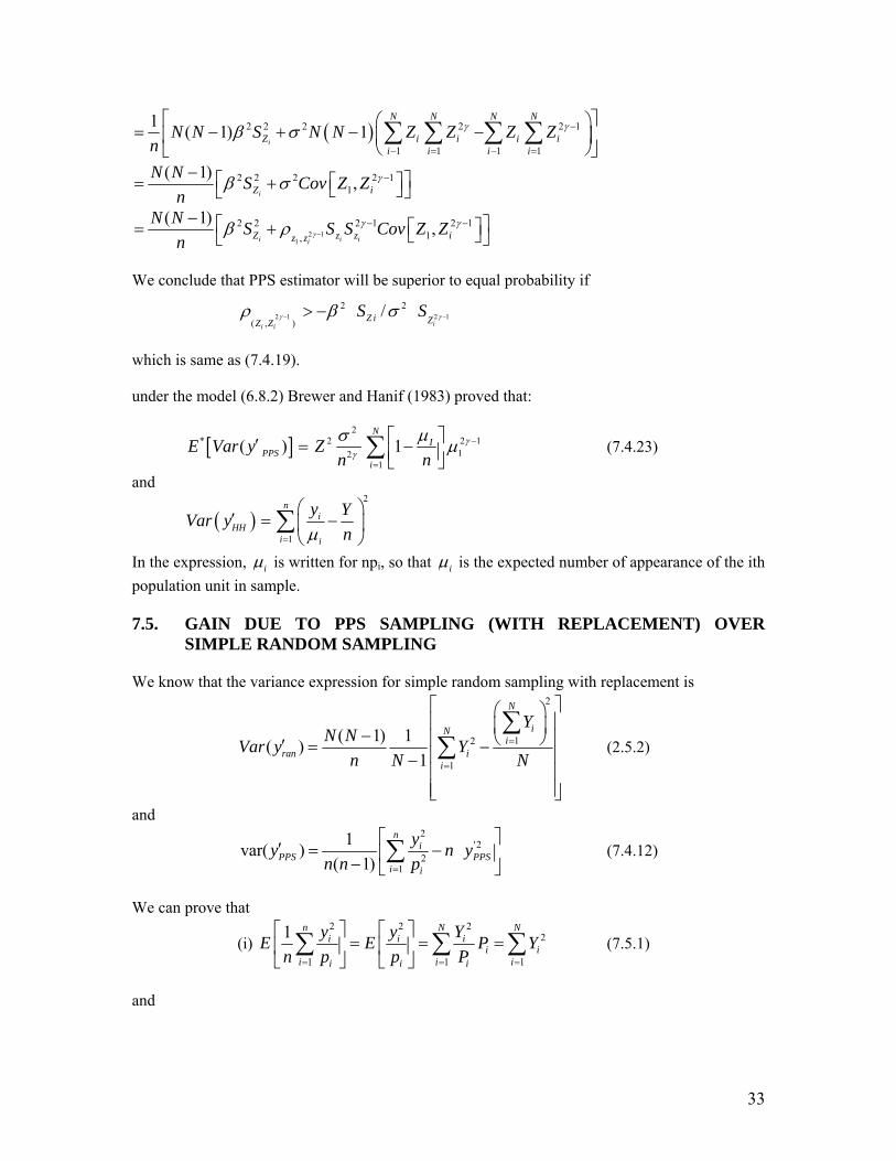
under the model (6.8.2) Brewer and Hanif (1983) proved that:

[ ]2

* 2 2 112

1

( ) 1N

IPPS

i

E Var y Zn n

γγ

µσ µ −

=

⎡ ⎤′ = −⎢ ⎥⎣ ⎦∑ (7.4.23)

and

( )2

1

ni

HHi i

y YVar ynµ=

⎛ ⎞′ = −⎜ ⎟

⎝ ⎠∑

In the expression, iµ is written for npi, so that iµ is the expected number of appearance of the ith population unit in sample.

7.5. GAIN DUE TO PPS SAMPLING (WITH REPLACEMENT) OVER

SIMPLE RANDOM SAMPLING We know that the variance expression for simple random sampling with replacement is

2

12

1

( 1) 1( )1

N

iNi

ran ii

YN NVar y Y

n N N=

=

⎡ ⎤⎛ ⎞⎢ ⎥⎜ ⎟− ⎝ ⎠⎢ ⎥′ = −⎢ ⎥−⎢ ⎥⎢ ⎥⎣ ⎦

∑∑ (2.5.2)

and 2

'22

1

1var( )( 1)

ni

PPS PPSi i

yy n yn n p=

⎡ ⎤′ = −⎢ ⎥− ⎣ ⎦

∑ (7.4.12)

We can prove that

(i) 2 2 2

2

1 1 1

1 n N Ni i i

i ii i ii i i

y y YE E P Yn p p P= = =

⎡ ⎤ ⎡ ⎤= = =⎢ ⎥ ⎢ ⎥

⎣ ⎦ ⎣ ⎦∑ ∑ ∑ (7.5.1)

and

34

(ii)

( )

[ ]

'2 '2

2 2 2

1 1var( ) ( ) var

1 ( ) { ( )} { ( )} var

PPS PPS PPS PPS

pps pps PPS PPS

E y y E y E yN N

E y E y E y E yN

′ ′⎡ ⎤ ⎡ ⎤− = −⎣ ⎦ ⎣ ⎦

′ ′ ′ ′⎡ ⎤= − + −⎣ ⎦

221 ( ) ( )PPS PPS

YVar y Y Var yN N

′ ′⎡ ⎤= + − =⎣ ⎦2YN= . (7.5.2)

Using (7.5.1) and (7.5.2) in (2.5.2) we can have

( )2

'2

1

( 1) 1 1 1var ( ) var( )1

ni

PPS ran PPS PPSi i

yN Ny y yn N n p N=

⎡ ⎤−′ ′= − −⎢ ⎥− ⎣ ⎦∑ .

(7.5.3) 2

'22

1

1 1var ( ) var( )n

iPPS ran PPS PPS

i i

yNy y yn p n n=

′ ′= − +∑ .

2

'22

1

1 1 var( )n

iPPS PPS

i i

yN ny yn p n=

⎡ ⎤′= − +⎢ ⎥

⎣ ⎦∑ . (7.5.4)

Subtracting ( )var PPSy′ from (5.5.4) we get

2'2

21

1 1var ( ) var( ) var( ) var( )n

iPPS ran PPS PPS PPS PPS

i i

yy y N ny y yn p n=

⎡ ⎤′ ′ ′ ′− = − + −⎢ ⎥

⎣ ⎦∑ .

( )

2 22 2

2 21 1

1 1 11

n ni i

PPS PPSi ii i

y ynN ny nyn p n n n p= =

⎡ ⎤ ⎡ ⎤−′ ′= − + −⎢ ⎥ ⎢ ⎥−⎣ ⎦ ⎣ ⎦∑ ∑

22 2

22 2 2

1 1

1 1n nppsi i

PPSi ii i

yy yN yn p n n p n= =

′′= − − +∑ ∑ .

2 2

2 2 21 1

1n ni i

i ii i

y yNn p n p= =

= −∑ ∑

2

21

1 1ni

i i i

y Nn p p=

⎡ ⎤= −⎢ ⎥

⎣ ⎦∑ . (7.5.5)

35

Therefore

2

21

1 1ar ( ) ar( ) .n

iPPS ran PPS

i i i

yv y v y Nn p p=

⎛ ⎞′ ′− = −⎜ ⎟

⎝ ⎠∑ . (7.5.6)

An estimate of the percentage gain in efficiency due to pps sampling is ainin

var ( ) ar ( ) 100var ( )

PPS ran PPS

PPS

y v yy

′ ′−×

′. (7.5.7)

EXAMPLE (7.3)

A sample of size 5 has been selected from a population of size 20 farms. Number of trees,

along with initial probability of selection is given

i) Estimate the total number of trees in that area, calculate the estimated variance and

standard error of this estimator.

ii) Estimate the gain in precession over simple random sampling. The actual number of

trees are 28443.

S.No. of Villages

No. of Trees

(yi)

Probability of Selection

(pj)

i

i

yp

2

iPPS

i

y yp

⎛ ⎞′−⎜ ⎟

⎝ ⎠

2 /i iy p

8 4

16 11 10

311 949

11799 2483 3044

0.014 0.036 0.275 0.121 0.212

22214.286 26361.111 42905.455 20520.661 14358.490

9349614.91 1186162.77

310938735.20 22575222.29

119104700.50

6908642.9 25016694.4 506241458.1 50952801.6 43707245.28

126360.003 463154435.5 632826842.1

36

(i) Estimated Total 1

1 ni

PPSi i

yyn p=

′= = ∑ .

trees252725

003.126360==

Actual Total 28443Y ==

(ii) 2

1

1( ) .( 1)

ni

PPS PPSi i

yvar y yn n p−

⎛ ⎞′ ′= −⎜ ⎟− ⎝ ⎠

∑

[ ] 77.231577215.463154435.45

1=

×=

(iii) 247.4812)y(E.S PPS =′ 2

'22

1

1 1var ( ) var( )n

iPPS ran PPS PPS

i i

yy N n y yn p n=

⎡ ⎤′ ′= − +⎢ ⎥

⎣ ⎦∑ (7.5.4)

( )[ ] )77.23157721(51)25272(51.63282684220

251 2 +−=

= 383158187.5

ar ( ) ar ( )100

ar( )pps ran PPS PPS

PPS

v y v yv y′ ′−

×′

%56.155410077.23157721

77.231577215.383158187=×

−=

7.6. ALTERNATIVE ESTIMATOR TO HANSEN AND HURVITZ ESTIMATOR

Pathak (1962) described an estimator for the sampling scheme suggested by Hansen

and Hurvitz (1963). For this let we have a sample of three units selected from a

population of N units. Llet the selected sample has yi, yi, yj observations with

probabilities pi, , pi, pj respectively, then Pathak (1962) defines an estimator:

13

j i jip

i j i j

y y yyyp p p p

⎡ ⎤+′ = + +⎢ ⎥

+⎢ ⎥⎣ ⎦, (7.6.1)

37

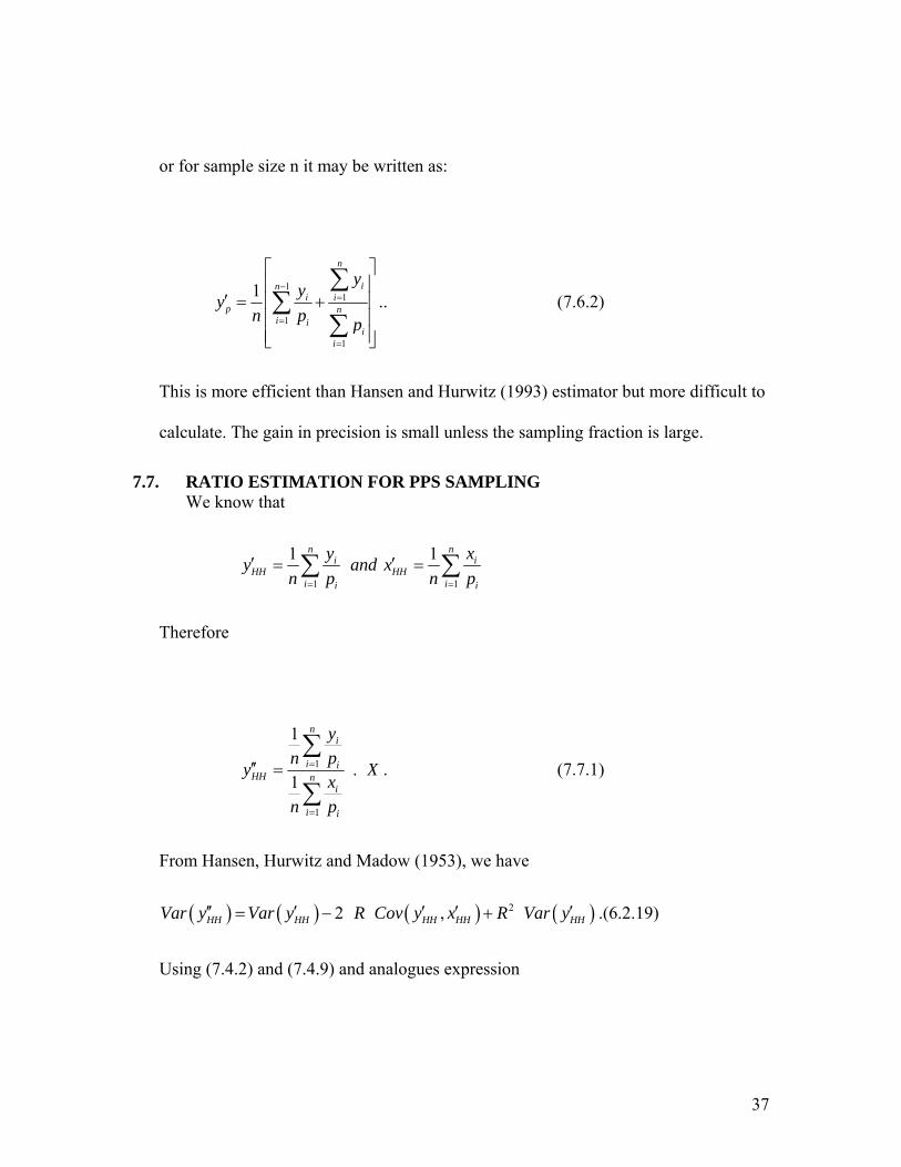
or for sample size n it may be written as:

11

1

1

1

n

ini i

p ni i

ii

yyy

n p p

−=

=

=

⎡ ⎤⎢ ⎥

′ = +⎢ ⎥⎢ ⎥⎢ ⎥⎣ ⎦

∑∑

∑.. (7.6.2)

This is more efficient than Hansen and Hurwitz (1993) estimator but more difficult to

calculate. The gain in precision is small unless the sampling fraction is large.

7.7. RATIO ESTIMATION FOR PPS SAMPLING We know that

1 1

1 1n ni i

HH HHi ii i

y xy and xn p n p= =

′ ′= =∑ ∑

Therefore

1

1

1

.1

ni

i iHH n

i

i i

yn py X

xn p

=

=

′′ =∑

∑. (7.7.1)

From Hansen, Hurwitz and Madow (1953), we have

( ) ( ) ( ) ( )22 ,HH HH HH HH HHVar y Var y R Cov y x R Var y′′ ′ ′ ′ ′= − + .(6.2.19)

Using (7.4.2) and (7.4.9) and analogues expression

38

2

1

1( )N

iHH i

i i

XVar x P Xn P=

⎛ ⎞′ = −⎜ ⎟

⎝ ⎠∑ , (7.7.2)

in (6.2.19) and on simplification

( )2 2

2 2

1 1 1

1 2 ( )N N N

i i i iHH

i i ii i i

Y Y X YVar y R R Y RXn P P P= = =

⎡ ⎤′′ = − + − −⎢ ⎥

⎣ ⎦∑ ∑ ∑ (7.7.3)

2

1

1 1 (N

i ii i

Y R Xn P=

⎡ ⎤= −⎢ ⎥

⎣ ⎦∑ . (7.7.4)

This may be put easily as

2

1

1( )N

i iHH i

i i i

Y XVar y P Rn P P−=

⎛ ⎞′′ = −⎜ ⎟

⎝ ⎠∑ . (7.7.5)

An approximate unbiased estimator of )y(Var HH′′ may be written in a straight forward

way or may be derived

2

1

1var( )( 1)

ni i

HHi i i

y xy rn n p p=

⎛ ⎞′′ = −⎜ ⎟− ⎝ ⎠

∑ , (7.7.6)

or

2

1

1var( )( 1)

Ni i

HHi i i

y xyyn n p x p=

⎛ ⎞′′′ = −⎜ ⎟′− ⎝ ⎠

∑ . (7.7.7)

CHAPTER-4

TWO-PHASE SAMPLING 1.1 Introduction

Consider the problem of estimating population mean of Y of a Study Variable Y from a finite population on N units. When information on one or more auxiliary variable say X and Z which are correlated with the variable Y are available or can be cheaply obtained ratio or regression type estimates can be used to improve the efficiency. These cases may include knowledge of X or Z or both X and Z . These are

39

however situations where prior knowledge about these may be lacking and a census or complete count is too costly. Two phase sampling is used to gain information about x & z cheaply from a first stage bigger sample. A sub sample is then selected from the units selected at the first phase & Y is observed for the selected units. Useful references in this area are Mohanty (1967), Chand (1975), Ahmed (1977), Kiregyera (1980, 1984), Sahoo et al (1993) and Roy (2003). We have used Linear models and the method of Least Squares (L.S) following Roy (2003) to deal with different situations. The results as expected are encouraging. We have also indicated how slight adjustments can be made in earlier works to improve the efficiency of the estimates. An implication of this is that some of these earlier works do not fully utilize the available information. Let N be the size of the population, from which a sample of size 1n ( 1n < N ) is drawn using a simple random sampling without replacement. The values of X and Z are noted for the quits selected. From this sample a sub-sample of size 2n ( 2 1n n< ) is again selected using a simple random sampling with out replacement observing as Y. S. Further let 2y , 2x and 2z be the sample means of y, x, and z variables respectively based on the sample of size 1n and let 2x and 2z be the sample mean based on the first phase sample of size 1n of variable x and z respectively. Various situations of interest may arise depending on availability of information about X and Z . We will deal with them separately.

To suit different situation we introduce the following notations. Let ( )22

1

11

Ny i

iS Y Y

N == −

−∑ ,

11

1 1n N

θ = − , 22

1 1n N

θ = − , 2 2 2y yC S Y= with 2 2,x zC C similarly defined. Also , andxy yz xzρ ρ ρ denote

the population correlation coefficient between andX Y , andY Z and andX Z respectively. We will also write

40

11 yy Y e= + ,

11 ,xx X e= + 11 zz Z e= + , ( )1

2 2 21x xE e X C= θ

( ) ( )1 1

2 2 2 2 2 21 1y y z yE e Y C and E e Z C= θ = θ . ( )x y y x xyE e e X Y C C= ρ

22 ,xx X e= + ( )2

2 2 22 ,x xE e X C= θ ( )2 2 2x y x y xyE e e X YC C= θ ρ

( ) ( )2

2 2 21 2 1x xE e e X C− = θ − θ ,

(4.1.1) ( ) ( )

2 1 2 2 1y x x y x xyE e e e Y X C C⎡ ⎤− = θ − θ ρ⎣ ⎦

( )1 20x z zE e e e⎡ ⎤− =⎣ ⎦

( )2 1 1y x y x xyE e e Y X C C= θ ρ

with other terms similarly defines: Also we will assume that both 1 2

,y ye e are much smaller in comparison with Y with similar assumptions for auxiliary variables we will look into the following situations separately.

i) In addition to the sample we are given the population means of X and Z which are X and Z respectively. We may call this complete information case.

ii) In addition to the sample we are given X only, ( Z being unknown). We will call this partial information case.

iii) Only the information on the sample is available i.e. X and Z are unknown. We will call this no additional information case.

4.2 Ratio and Regression Estimators

In this section following estimator of ratio and regression alongwith mean square error have been considered.

a) ( )2

1 22

yT X

x= [ X is known ]

b) ( )2

12 22

yT x

x= [ no information ]

c) ( ) ( )2 1 23 2 yxT y b x x= + − [ no information ]

4.2.1 Ratio Estimator with known information

Consider

( )2

1 22

yT X

x=

(4.2.1)

Using (1.1.1) we get

41

( )2

2

2 2

2 2

2 2

1 2 .

1 1

1

y

x

y x

y x

y x

Y eT X

X e

e eY

Y X

e eY

Y X

YY e eX

+=

+

⎛ ⎞⎛ ⎞= + −⎜ ⎟⎜ ⎟⎜ ⎟⎜ ⎟

⎝ ⎠⎝ ⎠⎛ ⎞

= + −⎜ ⎟⎜ ⎟⎝ ⎠

= + −

( ) 2 2y xYT Y e eX

⎛ ⎞− = −⎜ ⎟

⎝ ⎠

The mean square error of ( )1 2T will be

( )( ) ( )( ) 2 2

22

1 2 1 2 y xYMSE T E T Y E e eX

⎛ ⎞= − = −⎜ ⎟

⎝ ⎠

(4.2.2)

Taking the square R.H.S of (4.2.2.) we get

2 2 2 2

22 2

2 2y x y xY YE e e e e

XX

⎡ ⎤= + −⎢ ⎥

⎢ ⎥⎣ ⎦

Using (1.1.1)

MSE ( )( )1 2T2

2 2 2 22 2 22 2y x y x xy

Y YY C X C Y X C CXX

= θ + θ − θ ρ

On simplification we get

( ) ( )( )1 2 1 2V MSE T= 2 2 22 2y x xy x yY C C C C⎡ ⎤= θ + − ρ⎣ ⎦

(4.2.3) 4.2.2 Ratio Estimator with no information

Consider

( )2

12 22

yT x

x=

(4.2.4)

Using (1.1.1) in (4.2.4) we get

( ) ( )2

12

2 2y

xx

Y eT X e

X e

+= +

+

42

( ) ( ) ( )

( )

( )

( )

2 1 2

1 2

2

1 2

2

2 1 2

1

1 1

1

y x x

x xy

x xy

y x x

Y e X e X e

e eY e

X X

e eY e

X X

YY e e eX

−= + + +

⎛ ⎞⎛ ⎞= + + −⎜ ⎟⎜ ⎟⎜ ⎟⎜ ⎟

⎝ ⎠⎝ ⎠⎛ ⎞

= + + −⎜ ⎟⎜ ⎟⎝ ⎠

= + + −

or

( ) ( )2 1 22 2 y x xYT Y e e eX

− = + −

The mean square error of ( )2 2T

( )( ) ( )( ) ( )2 1 2

2

2 2 2 2 y x xYMSE T E T Y E e e eX

⎡ ⎤= − = + −⎢ ⎥

⎣ ⎦

(4.2.5)

( ) ( )2 1 2 2 1 2

2 222 2y x x y x x

Y YE e e e e e eXX

⎡ ⎤= + − + −⎢ ⎥

⎢ ⎥⎣ ⎦

Using (1.1.1) we get

MSE ( )( )2 2T ( ) ( )2

2 2 2 22 1 2 2 12 2y x x y xy

Y YY C X C Y X C CXX

= θ + θ − θ + θ − θ ρ

( ) ( )2 2 2 2 22 1 2 1 22y x x y xyY C Y C Y C C= θ + θ − θ − θ − θ ρ

or ( ) ( )( )3 2 3 2MSEV T= ( )( )2 2 2

2 2 1 2y x x y xyY C C C C⎡ ⎤= θ + θ − θ − ρ⎣ ⎦

(4.2.6) 4.2.3 Regression Estimator with no information

Consider

( ) ( )2 1 23 2 yxT y b x x= + − (4.2.7)

Using (1.1.1) we get

( ) ( ) ( )

( )2 1 2

2 1 2

3 2 y yx r x x

y yx x x

T Y e e e e

Y e e e

= + β + −

= + + β −

or ( )( ) ( )2 1 22 2 y yx x xT Y e e e− = + β −

(4.2.8)

The mean square error of ( )3 2T is

( )( ) ( )( ) ( )2 1 2

2 2

3 2 3 2MSE y yx x xT T Y E e e e⎡ ⎤= − = + β −⎣ ⎦

(4.2.9) or

43

( )( ) ( )2 2 1 2

23 2MSE y yx y x xT E e e e e⎡ ⎤= + β −⎣ ⎦

(4.2.10) or ( )( ) ( )2 2

2 1 23 2MSE y yx y x xyT Y C Y X C C= θ + β θ − θ ρ

Substituting the value of xyyyx

x

Y CX C

ρβ =

( )( ) ( )2 22 1 23 2MSE xy y

y y x xyx

YCT Y C Y X C C

XCρ

= θ + θ − θ ρ

On simplification we get

( )( ) ( )2 2 22 1 23 2MSE y xyT Y C ⎡ ⎤= θ + θ − θ ρ⎣ ⎦

( ) ( )( ) ( )2 2 2 22 12 2 2 2MSE 1y xy xyV T Y C ⎡ ⎤= = θ − ρ + θ ρ⎣ ⎦

(4.2.11) 4.3 Mohanty’s [1967] Estimator and some modifications

In this section following estimators are mentioned.

a) ( ) ( )2 1 24 22

yxZT y b x xz

⎡ ⎤= + −⎣ ⎦

b) ( ) ( ) 12 1 25 2

2yx

zT y b x x

z⎡ ⎤= + −⎣ ⎦

c) ( ) ( )2 1 26 22

yzXT y b z zx

⎡ ⎤= + −⎣ ⎦

d) ( ) ( )21 17 2

2yx

zT z b X x

z⎡ ⎤= + −⎣ ⎦

4.3.1 Mohanty (1967) considered the estimation when Z is known

( ) ( )2 1 24 22

yxZT y b x xz

⎡ ⎤= + −⎣ ⎦

(4.3.1)

Using (1.1.1) in (4.3.1) we get

( ) ( ) ( )2 1 22

4 2 y yx r x xz

ZT Y e e e ez e

⎡ ⎤= + + β + −⎣ ⎦ +

On simplification we get

( ) ( )2 1 2 24 2 y yx x x zYT Y e e e eZ

= + + β − −

or

( ) ( )2 1 2 24 2 y yx x x zYT Y e e e eZ

− = + β − −

The MSE of ( )3 2T is

44

( )( ) ( )2 1 2 2

22

4 2 y yx x x zYE T Y E e e e eZ

⎡ ⎤− = + β − −⎢ ⎥

⎣ ⎦

(4.3.2)

( ) ( )

( )

2 1 2 2 2 1 2

2 2 2 1 2

222 2 22 2

2 2

y yx x x z yx y x x

y z yx z x x

YE e e e e e e eZ

Y Ye e e e eZ Z

⎡= + β − + + β −⎢

⎢⎣⎤

− − β − ⎥⎦

( ) ( )2

2 2 2 2 2 2 22 2 1 24 2 2MSE y yx x z

YT Y C X C Z CZ

⎡ ⎤ = θ + θ − θ β + θ⎣ ⎦

( )1 2 22 2yx y x xy y z yzYY X C C Y Z C CZ

+ θ − θ β ρ − θ ρ

( )1 22 yx z x xzY Z X C CZ

− θ − θ β ρ

(4.3.3)

Putting the values of xy yyx

x

C YX C

ρβ = in (4.3.3) we get

( )( ) ( )2 2 2

2 2 2 22 1 14 2 2 2

xy yy x

x

C YMSE T Y C X C

X C

ρ= θ + θ − θ

( )1 22 xy yy x xy

x

YCY X C C

X Cρ

+ θ − θ ρ

( )22 1 22 xy y

y z yz z x xzx

C Y YY C C Z X C CC X Z

ρ−θ ρ − θ − θ ρ (4.3.4)

On simplification

( )( ) ( ) ( )2 2 2 2 2 2 22 2 1 2 1 24 2 2y y xy z y xyMSE T Y C C C C⎡= θ + θ − θ ρ + θ + θ − θ ρ⎣

( )2 1 22 2y z yz y z xy xzC C C C ⎤− θ ρ − θ − θ ρ ρ ⎦

( ) ( )2 2 2 2 22 2 1 2 2 1 22 2y y xy z y z yz y z xy xzY C C C C C C C⎡ ⎤= θ − θ −θ ρ +θ − θ ρ − θ −θ ρ ρ⎣ ⎦

( )2 2 2 2 2 2 2 2 2

2 2 2 2 1 2y y yz y yz y xy zY C C C C C⎡= θ − θ ρ + θ ρ − θ − θ ρ + θ⎣

( )2 1 22 2y z y z xy xzC C C C ⎤− θ − θ − θ ρ ρ ⎦

or ( ) ( )2 2 2 2 2 2 2 2

2 21 2y yz z y z y yz y yzY C C C C C C⎡= θ − ρ + θ − + ρ − ρ⎣

( ) ( )2 2 2 22 2 1 1 22y yz y xy y z xy xzC C C C ⎤θ ρ − θ − θ ρ − θ − θ ρ ρ ⎦

or

( ) ( )22 2 2 2 22 21y xz z y yz y yzY C C C C⎡ ⎧ ⎫= θ − ρ + − ρ − θ ρ⎨ ⎬⎢ ⎩ ⎭⎣

45

( ) ( )2 2 2 22 2 1 1 22y yz y xy y z xy xzC C C C ⎤+θ ρ − θ − θ ρ − θ − θ ρ ρ ⎥⎦

or

( ) ( )

( ){ }

22 2 22

2 2 2 2 2 22 1

1

2

y xz z y yz

y xy y z xy xz z xz z xz

Y C C C

C C C C C

⎡ ⎧ ⎫= θ − ρ + − ρ⎨ ⎬⎢ ⎩ ⎭⎣⎤+ θ − θ ρ + ρ ρ − ρ + ρ ⎥⎦

or

( ) ( )( ) ( ) ( )22 2 224 2 4 2 1y xz z y yzV MSE T Y C C C⎡ ⎧ ⎫= = θ − ρ + − ρ⎨ ⎬⎢ ⎩ ⎭⎣

( ) ( ){ }2 2 22 1 z xz y xy z xzC C C ⎤+ θ − θ ρ − ρ − ρ ⎥⎦

(4.3.5)

4.3.2 Mohanty’s Ratio-Cum-Regression Estimator with no Information

Mohanty (1967) constructed another Ratio-Cum-Regression estimator when sample

information are only given i.e.

( ) ( ) 12 1 25 2

2yx

zT y b x x

z⎡ ⎤= + −⎣ ⎦

(4.3.6)

Using (1.1.1) we get

( ) ( ) 1

2 1 22

5 2z

y yx r x xz

Z eT Y e B e e e

Z e

⎡ ⎤+⎡ ⎤⎡ ⎤= + + + − ⎢ ⎥⎣ ⎦⎣ ⎦ +⎢ ⎥⎣ ⎦

or

( ) ( ) 1 2

2 1 25 2 1 1z zy yx x x

e eT Y e B e e

Z Z

⎡ ⎤⎛ ⎞⎛ ⎞⎡ ⎤= + + − + −⎢ ⎥⎜ ⎟⎜ ⎟⎜ ⎟⎜ ⎟⎣ ⎦ ⎢ ⎥⎝ ⎠⎝ ⎠⎣ ⎦

The mean square error of ( )5 2T is

( )( ) ( ) ( )2 1 2 1 2

22

5 2 y yx x x z zYE T Y E e e e e eZ

⎡ ⎤− = + β − + −⎢ ⎥

⎣ ⎦

(4.3.7)

( )( ) ( ) ( )

( ) ( ) ( ) ( )

2 1 2 1 2

2 1 2 2 1 2 1 2 1 2

22 22 25 2 2MSE

2 2 2

y yx x x z z

yx y x x y z z yx x x z z

YT E e e e e eZ

Y Ye e e e e e e e e eZ Z

⎡= + β − + −⎢

⎢⎣⎤

+ β − + − + β − − ⎥⎦

Using (1.1.1) we get

46

( )( ) ( ) ( )

( ) ( )

22 2 2 2 2 2 2

2 2 1 2 15 2 2

1 2 2 1

MSE

2 2

y yx x z

yx y x xy y z yz

YT Y C X C Z CZ

YY X C C Y Z C CZ

= θ + β θ − θ + θ − θ

+ θ − θ β ρ + θ − θ ρ

( )2 12 yx x z yzX Z C C+ β θ − θ ρ (4.3.8)

Putting the value of yyx xy

x

YCXC

β = ρ

( )( ) ( ) ( )2 2 2 2

2 2 2 2 2 22 2 1 2 15 2 2 2 2

xy yy x z

x

C Y YMSE T Y C X C Z CC X Z

ρ= θ + θ − θ + θ − θ

( ) ( )

( )

2 1 2 1

2 1

2 2

2

xy yy x xy y z yz

x

xy yx z xy yz

x

C Y YY X C C Y Z C CX C Z

C YX Y C C

X C

ρ+ θ − θ ρ + θ − θ ρ

ρ+ θ − θ ρ ρ

On simplification we get

( )( ) ( ) ( )2 2 2 2 2 2 2 22 2 15 2 2y y xy z xz y z xy xz z xzMSE t Y C C C C C C⎡= θ + θ − θ − ρ − ρ + ρ ρ + ρ⎣

2 2 2 2 22z y yz y z yz y yzC C C C C ⎤+ + ρ − ρ + ρ ⎦

( )2 2 2 2 2 2 22 2 1 2y xy y z xy yY C C C C⎡ ⎤ ⎡= θ + θ − θ ρ + − ρ⎣ ⎦ ⎣

2 2y z yz y z xy xzC C C C ⎤− ρ + ρ ρ ⎦

( )2 2 2 2 22 2 1 2 2y xy y z y z yz y z xy xzY C C C C C C C⎡ ⎤ ⎡ ⎤= θ + θ − θ −ρ − − ρ + ρ ρ⎣ ⎦ ⎣ ⎦

( ) ( )( ) ( ) ( )22 2 2 22 2 15 2 5 2MSE y xz z xy y xz zV T Y C C C C

⎡⎡ ⎤= = θ + θ − θ ρ − ρ − ρ⎢⎣ ⎦ ⎣

( )2 2 2z y yz y xzC C C ⎤+ − ρ − ρ ⎥⎦

(4.3.9) 4.3.3 Modification of ( )4 2T by Interchanges X and Z

( ) ( )2 1 26 22

yzXT y b z zx

⎡ ⎤= + −⎣ ⎦

(4.3.10)

Using (1.1.1) in (4.3.10) we get

( ) ( ) ( )2 1 22

6 2 y yz z z zx

XT Y e e e eX e

⎡ ⎤= + + β + −⎣ ⎦ +

( ) 2

2 1 21 x

y yz z ze

Y e e eX

⎛ ⎞⎡ ⎤= + + β − −⎜ ⎟⎜ ⎟⎣ ⎦ ⎝ ⎠

47

( ) ( )2 2 1 26 2 x y yz z zYT Y e e e eX

= − + + + β −

or

( ) ( )2 1 2 26 2 y yz z z xYT Y e e e eX

− = + β − −

The mean square error of ( )6 2T is

( )( ) ( )( ) ( )2 1 2 2

2

6 2 7 2 y yz z z xYMSE T E T E e e e eX

⎡ ⎤= = + β − −⎢ ⎥

⎣ ⎦

(4.3.11)

Squaring the R.H.S of (4.3.11)

( )( ) ( ) ( )2 1 2 2 2 1 2

22 2 2

6 2 2 2y yz z z x yz y z zYMSE T e e e e e e eX

⎡= + β − + + β −⎢⎢⎣

( )2 2 2 1 22 2y x yz x z z

Y Ye e e e eX X

⎤− − β − ⎥

⎦

Using (1.1.1)

( )( ) ( )2

2 2 2 2 2 22 2 1 26 2 2y yz x

YMSE T Y C Z X CX

= θ + θ − θ β + θ

( )1 2 2 yz y z y z yzY ZC C C C+ θ − θ β ρ

( )2 1 22 2y z xy yz x z xzY YY X C C X Z C CX X

− θ ρ − θ − θ β ρ

Putting the value of 2

22

yyz yz

z

Y C

Z eβ = ρ

( )( ) ( )2 2 2 2

2 2 2 22 2 1 26 2 2 2 2

yz yy x

z

Y C YMSE T Y C X CZ C X

ρ= θ + θ − θ + θ

( )1 22 yz yy z yz

z

Y CY Z C C

Z C

ρ+ θ − θ ρ

( )2 1 22 2 .yz yy x xy x z y z xz

z

Y CY YY X C C X Z C C C CX Z C X

ρ− θ ρ − θ − θ ρ

or ( )2 2 2 2 2

2 1 1 2 22y y xz x y x xyY C C C C C⎡= θ + θ − θ ρ + θ − θ ρ⎣

( )1 22 yz xz y xC C ⎤− θ − θ ρ ρ ⎦

( ) ( )2 2 2 22 2 1 2 1 22y y xz y x xy yz xz y xY C C C C C C⎡ ⎤= θ + θ − θ ρ + θ ρ − θ − θ ρ ρ⎣ ⎦

( ){ } { }2 2 2 2 22 2 1 2 2y y xz x y yz xz x y x xyY C C C C C C C⎡ ⎤= θ + θ − θ ρ + ρ ρ + θ − ρ⎣ ⎦

48

( )( )2 2 2 2 2 2 2 22 2 1 2y y xz x yz x y yz xz x yzY C C C C C C⎡= θ + θ − θ ρ + ρ − ρ ρ − ρ⎣

( )2 2 2 2 22 2x y xy y x xy y xyC C C C C ⎤+θ + ρ − ρ − ρ ⎦

( ) ( ) ( )22 2 2 22 2 16 2 y x xy y xy x yzMSE T Y C C C C⎡ ⎤⎡ ⎤ = θ + θ − θ ρ − ρ − ρ⎢ ⎥⎣ ⎦ ⎣ ⎦

( )2 22 x y xy y xyC C C⎡ ⎤+θ − ρ − ρ⎢ ⎥⎣ ⎦

(4.3.12) 4.3.4 Modification of Mohanty when X is known

( ) ( )21 17 2

2yx

yT z b X x

z⎡ ⎤= + −⎣ ⎦

(4.3.13)

Using (1.1.1) in (4.3.13) we get

( ) ( )2

1 1

2

7 2 1yz yx x

z

Y eT Z e e

Z e

+⎡ ⎤= + +β −⎣ ⎦+

( )2 1 1

11 1

y z zyx x

Y e e eZ e

Z Z Z

+ ⎡ ⎤⎛ ⎞ ⎛ ⎞= − + − β⎢ ⎥⎜ ⎟ ⎜ ⎟⎜ ⎟ ⎜ ⎟⎢ ⎥⎝ ⎠ ⎝ ⎠⎣ ⎦

( ) 1 2 1 2

21 1 1z z x z

y yxe e e e

Y eZ Z Z Z

⎡ ⎤⎛ ⎞⎛ ⎞ ⎛ ⎞= + + − − β −⎢ ⎥⎜ ⎟⎜ ⎟ ⎜ ⎟⎜ ⎟⎜ ⎟ ⎜ ⎟⎢ ⎥⎝ ⎠⎝ ⎠ ⎝ ⎠⎣ ⎦

( ) 1 2

2 11 z z

y yx xe e

Y e eZ Z

⎡ ⎤= + + − − β⎢ ⎥

⎢ ⎥⎣ ⎦

or

( )2 1 2 1y z z yx xY YY e e e eZ Z

= + − − β

( ) ( )2 1 2 17 2 y z z yx xY YT Y e e e eZ Z

− = + − − β

Mean square error of ( )7 2T is

( )( ) ( )( ) ( )2 1 2 1

22

7 2 7 2 y z z yx xY YMSE T E T Y E e e e eZ Z

⎡ ⎤= − − + − − β⎢ ⎥

⎣ ⎦

(4.3.14)

( )2 1 2 1

2 222 2 22 2y z z yx x

Y YE e e e eZ Z

⎡= + − + β⎢

⎢⎣

( ) ( )2 1 2 2 1 1 1 2

2

22 2y z z yx y x yx x z zY Y Ye e e e e e e eZ Z Z

⎤+ − − β − β − ⎥

⎥⎦

( ) ( )2 2

2 2 2 2 2 22 2 1 1 22 2 2y z x y z yz

Y Y YY C Z C X C YC ZCZZ Z

= θ + θ − θ + + θ − θ ρ

49

12 yz y x yxY Y X C CZ

− θ β ρ

On simplification we get

( )( ) ( )2

2 2 2 2 22 2 1 17 2 2y z yx x

XMSE T Y C C CZ

⎡= θ + θ − θ + θ β⎢

⎢⎣

( )1 2 12 2y z yz y z yxXC C C CZ

⎤+ θ − θ − θ β ρ ⎥

⎦

Putting the value of yxβ

( )( ) ( )2 2 2 2

2 2 2 22 1 17 2 2 2 2

xy yy z x

x

Y C XMSE T Y C C CX C Z

⎡ ρ⎢= + θ − θ + θ⎢⎣

( )1 2 12 2 yy z yz xy y x yz

x

Y CXC C C CZ X C

⎤+ θ − θ ρ − θ ρ ρ ⎥

⎥⎦

or

( )1

22 2 2 2

2 2 1 1 2y z y xyYY e C CZ

⎡= θ + θ − θ + θ ρ⎢

⎢⎣

( ) 21 2 12 2y z yz y xy yz

YC C CZ

⎤+ θ − θ ρ − θ ρ ρ ⎥

⎦

or

( ) { }2 2 2 2 2 2 22 2 1 2y z y z xz y yx y xyY C C C C C C

⎡= θ + θ − θ − ρ + ρ − ρ⎢

⎣

2

2 2 22 2 2y xy y xy yz

Y YC CZZ

⎤⎧ ⎫⎪ ⎪+θ ρ − ρ ρ ⎥⎨ ⎬⎪ ⎪⎥⎩ ⎭⎦

or

( ) ( )22 2 2 22 2 1y z y xy y yxY C C C C

⎡ ⎧ ⎫= θ + θ − θ − ρ − ρ⎨ ⎬⎢⎩ ⎭⎣

2

2 2 2 2 21 2 2y xy yz yz y xy yz

Y YC CZZ

⎤⎧ ⎫⎪ ⎪+θ ρ + ρ − ρ − ρ ρ ⎥⎨ ⎬⎪ ⎪⎥⎩ ⎭⎦

or

( )( ) ( ) ( )22 2 2 22 2 17 2 y z y xy y xyMSE T Y C C C C

⎡ ⎧ ⎫= θ + θ − θ − ρ − ρ⎢ ⎨ ⎬

⎢ ⎩ ⎭⎣

2

21 y xy yz yz

Y CZ

⎤⎧ ⎫⎛ ⎞⎪ ⎪⎥+θ ρ − ρ − ρ⎨ ⎬⎜ ⎟ ⎥⎝ ⎠⎪ ⎪⎩ ⎭⎦

(4.3.15) 4.4 Chand’s (1975) Estimators

In this section following estimator are derived

a) ( )1

28 22 1

x ZT yx z

=

50

b) ( )2 1

29 21

x zT y

x Z=

c) ( )1 1

210 22

z xT y

z X=

d) ( )1

211 22 1

z XT yz x

=

4.4.1 Chand (1975) suggested chain-based ratio and product estimator-I

( )1

28 22 1

x ZT yx z

=

(4.4.1)

Using (1.1.1) in (4.4.1) we get

( ) ( ) 1

22 1

8 2x

yx z

X e ZT Y eX e Z e

+= +

+ +

( )

( )

( )

1 2 1

2

1 1 1

2

1 2 1 2

1 1 1

1

x x zy

x x zy

x x z y

e e eY e

X X Z

e e eY e

X X Z

Y YY e e e eX Z

⎛ ⎞⎛ ⎞⎛ ⎞= + + − −⎜ ⎟⎜ ⎟⎜ ⎟⎜ ⎟⎜ ⎟⎜ ⎟

⎝ ⎠⎝ ⎠⎝ ⎠⎛ ⎞

= + + − −⎜ ⎟⎜ ⎟⎝ ⎠

= + − − +

or

( ) ( )2 1 2 18 2 y x x zY YT Y e e e eX Z

− = + − −

The mean square of ( )8 2T will be

( )( ) ( )2 1 2 1

22

8 2 y x x zY YE T Y E e e e eX Z

⎡ ⎤− = + − −⎢ ⎥

⎣ ⎦

(4.4.2)

Squaring the R.H.S. of (4.4.2)

( ) ( )

( )

2 1 2 1 2 1 2

2 1 1 2 1

2 222 22 2

2

2

2 2

y x x z y x x

y z x x z

Y Y YE e e e e e e eXX Z

Y Ye e e e eZ XZ

⎡= + − + + −⎢

⎢⎣⎤

− − − ⎥⎥⎦

Using (1.1.1) we get

( )( ) ( )2 2

2 2 2 2 22 1 18 2 2 2MSE y x z

Y YT Y C X C Z CX Z

= θ + θ − θ + θ

( )1 2 12 2 0y x xy y z yzY YY X C C Y Z C CX Z

+ θ − θ ρ − θ ρ −

( )( ) ( )2 2 2 22 2 1 18 2MSE y x zT Y C C C⎡= θ + θ − θ + θ⎣

51

( )1 2 12 2y x xy y z yzC C C C ⎤+ θ − θ ρ − θ ρ ⎦

( ){ }2 2 2 2 2 2 2

2 2 1

21 1

2

2

y x xy y y x xy xy y

z y z yz

Y C C C C C C

C C C

⎡= θ + θ − θ + ρ − ρ − ρ⎣⎤+θ − θ ρ ⎦

( ) ( )( ) ( ) ( ){ }22 2 2 22 2 18 2 8 2V =MSE y x y xy y xyT Y C C C C⎡= θ + θ − θ − ρ − ρ⎢⎣

( ){ }2 2 21 z y yz y yzC C C ⎤+θ − ρ − ρ ⎥⎦

(4.4.3) 4.4.2 Chand (1975) Chain-based Ratio and Product Estimator-II

Chand (1975) considered another chain-based ratio estimator

( )2 1

29 21

x zT y

x Z=

(4.4.4)

Using (1.1.1) in (4.4.4) we get

( ) ( ) 2 1

21

9 2x z

yx

X e Z eT Y e

X e Z

+ += +

+

( )

( )

2 1 1

2

2 1 3 1

1 1 1x x zy

y x x z

e e eY e

X X Z

Y YY e e e eX Z

⎛ ⎞⎛ ⎞⎛ ⎞= + + − +⎜ ⎟⎜ ⎟⎜ ⎟⎜ ⎟⎜ ⎟⎜ ⎟

⎝ ⎠⎝ ⎠⎝ ⎠

= + − − +

( ) ( )2 1 2 19 2 y x x zY YT Y e e e eX Z

− = − − +

The mean square error of ( )9 2T is

( )( ) ( )( ) ( )2 1 2 1

22

9 2 9 2MSE y x x zY YT E T Y E e e e eX Z

⎡ ⎤= − = − − +⎢ ⎥

⎣ ⎦

(4.4.5)

( ) ( )2 1 2 1 2 1 2

2 222 22 2 2y x x z y x x

Y Y YE e e e e e e eXX Z

⎡= + − + − −⎢

⎢⎣

( )2 1 1 2 1

22 2y z x x z

Y Ye e e e eZ XZ

⎤+ − − ⎥

⎥⎦

(4.4.6)

Using (1.1.1) in (4.4.6) we get

( )( ) ( )2 2

2 2 2 2 2 22 2 1 19 2 2 2y x z

Y YMSE T Y C X C Z CX Z

= θ + θ − θ + θ

( )1 2 22 2 0y x xy y z yzY YY X C C C C Y ZX Z

− θ − θ ρ + θ ρ +

or

52

( ) ( )2 2 2 22 2 1 1 2 1 12 2y x z y x xy y z yzY C C C C C C C⎡ ⎤= θ + θ − θ + θ + θ − θ ρ + θ ρ⎣ ⎦

or ( ) ( ) ( )2 2 2 2

2 2 1 12 2y x y x xy z y z yzY C C C C C C C⎡ ⎤= θ + θ − θ + ρ + θ + ρ⎣ ⎦

( ) ( )( ) ( ) ( ){ }22 2 2 22 2 19 2 9 2MSE y x xy y y xyV T Y C C C C⎡= = θ + θ − θ + ρ − ρ⎢⎣

( )2 2 21 z yz z yz zC C C ⎤+θ + ρ − ρ ⎥⎦

(4.4.7) 4.4.3 Modification of Chand’s ( )9 2T

Following additional estimator parallel to Chand (1975) estimator is considered

( )1 1

210 22

z xT y

z X=

(4.4.8)

Using (1.1.1) in (4.3.8) we get

( ) ( ) 1

22 1

10 2z

yz x

Z e XT Y eZ e X e

+= +

+ +

( ) 1 2 1

21 1 1z z x

ye e e

Y eZ Z X

⎛ ⎞⎛ ⎞⎛ ⎞= + + + +⎜ ⎟⎜ ⎟⎜ ⎟⎜ ⎟⎜ ⎟⎜ ⎟

⎝ ⎠⎝ ⎠⎝ ⎠

( )2 1 2 1y z z xY YY e e e eZ Z

= + − −

( ) ( )2 1 2 110 y z z xY YT Y e e e eZ Z

− = + − −

The mean square error of ( )10 2T is

( )( ) ( )2 1 2 1

2

10 2 y z z xY YE T Y e e e eZ Z

⎡ ⎤− = + − −⎢ ⎥

⎣ ⎦

(4.4.9)

( ) ( )2 1 2 1 2 1 2

2 222 22 2y z z x y z z

Y Y YE e e e e e e eZZ Z

⎡= + − + + −⎢

⎢⎣

( )2 1 1 1 2

2

22 2y x x z zY Ye e e e eZ Z

⎤− − − ⎥

⎥⎦

(4.4.10)

Using (1.1.1) in (4.4.10) we get

( )( ) ( )2 2

2 2 2 2 2 22 2 1 210 2 2 2y z x

Y YMSE T Y C Z C X CZ Z

= θ + θ − θ + θ

( )1 2 12 2 0y z yz y x xyY YY Z C C Y XC CZ Z

+ θ − θ ρ − θ ρ +

53

( ) ( )2 2 2 22 2 1 1 1 2 12 2y z x y z yz y x xyY C C C C C C C⎡ ⎤= θ + θ − θ + θ + θ − θ ρ − θ ρ⎣ ⎦

( ){ }2 2 2 2 2 2 22 2 1 2y z y z yz y yz y yzY C C C C C C⎡= θ + θ − θ − ρ + ρ − ρ⎣

{ }2 2 2 2 21 2x y x xy y xy y xyC C C C C ⎤−θ − ρ + ρ − ρ ⎦

or

( ) ( )( ) ( ) ( )22 2 2 22 2 110 2 10 2 y z y yz y yzV MSE T Y C C C C⎡ ⎧ ⎫= = θ + θ − θ − ρ − ρ⎨ ⎬⎢ ⎩ ⎭⎣

( )2 2 21 x y xy y xyC C C ⎤⎧ ⎫+θ − ρ − ρ⎨ ⎬⎥⎩ ⎭⎦

(4.4.11) 4.4.4 Modification of Chand’s ( )8 2T

( )1 1

211 22

z xT y

z X=

(4.4.12)

Using (1.1.1) in (4.4.12) we get

( ) 1 1

22

.z xy

z

Z e X eY e

Z e X

+ += +

+

( ) 1 2 1

21 1 1z z x

ye e e

Y eZ Z X

⎛ ⎞⎛ ⎞⎛ ⎞= + + + +⎜ ⎟⎜ ⎟⎜ ⎟⎜ ⎟⎜ ⎟⎜ ⎟

⎝ ⎠⎝ ⎠⎝ ⎠

( ) ( )2 1 2 111 2 y z z xY YT Y e e e eZ Z

= + + − +

( ) ( )2 1 2 111 2 y z z xY YT Y e e e eZ Z

− = + − +

The mean square error of ( )11 2T is

( )( ) ( )( ) ( )2 1 2 1

22

11 2 11 2 y z z xY YMSE T T Y E e e e eZ Z

⎡ ⎤= − = + − +⎢ ⎥

⎣ ⎦

(4.4.13)

( )( ) ( )2 1 2 1

2 22 2

11 2 2 2y z z xY YMSE T E e e e eZ Z

⎡= + − +⎢

⎢⎣

( ) ( )1 2 2 1 1 2

2

22 2z z y x z zY Y Ye e e e e eZ Z Z

⎤+ − + + − ⎥

⎥⎦ (4.4.14)

Using (1.1.1) in (4.4.14) we get

( )( ) ( )2 2

2 2 2 2 2 22 2 1 111 2 2 2y z x

Y YMSE T Y C Z C X CZ Z

= θ + θ − θ + θ

54

( )2 1 12 2 0y z yz y z xyY YY Z C C Y X C CZ X

− θ − θ ρ + θ ρ +

On simplification we get

( )( ) ( )2 2 2 22 2 1 111 2 y z xMSE T Y C C C⎡= θ + θ − θ + θ⎣

( )2 1 12 2y z yz y x x xyC C C C ⎤+ θ − θ ρ + θ ρ ρ ⎦

( ){ } { }2 2 2 22 2 1 12 2y z y z yz x y x xyY C C C C C C C⎡ ⎤= θ + θ − θ + ρ + θ + ρ⎣ ⎦

( ) ( )( ) ( ) ( )22 2 22 2 111 2 10 2 y z y yz y yzV MSE T Y C C C C⎡ ⎧ ⎫= = θ + θ − θ + ρ − ρ⎨ ⎬⎢ ⎩ ⎭⎣

( ){ }2 21 x y xy y xyC C C ⎤

+θ + ρ − ρ ⎥⎦

(4.4.15) 4.5 Kiregyera’s Estimators and some modifications

Kiregyera (1980, 1984) suggested the following estimators:

a) ( ) ( )21 112 2

2xz

yT x b Z z

x⎡ ⎤= + −⎣ ⎦

b) ( )1

2 213 21

yxx

T y b Z xz

⎡ ⎤= + −⎢ ⎥

⎣ ⎦

c) ( ) ( ) ( )2 1 2 114 2 yx xzT y b x x b z Z⎡ ⎤= + − + −⎣ ⎦

The following estimators on the lines of Kiregyera’s are also been suggested to meet the requirements of this monographs:

d) ( ) ( )21 115 2

2zx

yT z b X x

z⎡ ⎤= + −⎣ ⎦

e) ( )1

2 216 21

yzz

T y b X zx

⎡ ⎤= + −⎢ ⎥

⎣ ⎦

4.5.1 Kiregyera’s (1980) Estimator (Chand-Kiregyera Estimator)

This is a modification of Chand (1975). Kiregyera (1980) assumed that iZ is closely related to iX , but compared to iX is remotely related to iY . This assumption may not always be to realize in particular. Therefore ( )8 2T may not be effectively used in many situations

( ) ( )21 112 2

2xz

yT x b Z z

x⎡ ⎤= + −⎣ ⎦

(4.5.1)

Using (1.1.1) in (4.5.1) we get

( ) ( ) ( )2

1 12

12 2y

x xz r zx

Y eT X e e Z Z e

X e

+⎡ ⎤= + + β + − −⎣ ⎦+

55

( )

( )

2 1

2 1

2 1 1

2

2 1 1

2

2

2 1 1

11 1 1

1 1

1

x xy xz z

x x zy xz

x x zy xz

xy x xz z

e eY e X e

X X X

e e eY e

X X X

e e eY Y e

X X X

e Y YY Y e e eX X X

− ⎡ ⎤⎛ ⎞ ⎛ ⎞= + + + − β⎢ ⎥⎜ ⎟ ⎜ ⎟⎜ ⎟ ⎜ ⎟⎢ ⎥⎝ ⎠ ⎝ ⎠⎣ ⎦

⎡ ⎤⎛ ⎞ ⎛ ⎞= + − + − β⎢ ⎥⎜ ⎟ ⎜ ⎟⎜ ⎟ ⎜ ⎟⎢ ⎥⎝ ⎠ ⎝ ⎠⎣ ⎦⎡ ⎤ ⎡ ⎤

= − + + − β⎢ ⎥ ⎢ ⎥⎢ ⎥ ⎢ ⎥⎣ ⎦ ⎣ ⎦⎡ ⎤

= − + + − β⎢ ⎥⎢ ⎥⎣ ⎦

( ) ( )2 1 2 112 2 y x x xz zY YT Y e e e eX X

= + + − − β

( ) ( )2 1 2 112 2 y x x xz zY YT Y e e e eX X

− = + − − β

(4.5.2)

The mean square error of ( )12 2T

( )( ) ( )2 1 2 1

22

12 2 y x x xz zY YE T Y E e e e eX X

⎡ ⎤− = + − − β⎢ ⎥

⎣ ⎦

(4.5.3)

( ) ( )2 1 2 1 2 1 2

222 2 22

2y x x xz z y x x

Y Y YE e e e e e e eX XX

⎡= + − + β + −⎢

⎢⎣

( )2 1 1 1 2

2

22 2xz y z xz z z zY Ye e e e eX X

⎤− β − β − ⎥

⎥⎦

(4.5.4)

Using (1.1.1) in (4.5.4) we get

( )( ) ( )2 2

2 2 2 2 2 2 22 2 1 112 2 2 2y x xz z

Y YMSE T Y C X C Z CX X

= θ + θ − θ + θ β

( )1 2 12 2 zeroy x xy xz y x yzY YY X C C Y C Z CX X

+ θ − θ ρ − θ β ρ +

(4.5.5)

Putting the Values of xxz xz

z

XCZ C

β = ρ in (4.5.5) we get

( )( ) ( )

( )

2 2 2 2 22 2 1 112 2

1 2 1

MSE

2 2

y x xz z

y x xy xz yz y x

T Y C C C

C C C C

⎡= θ + θ − θ + θ ρ⎣

⎤+ θ − θ ρ − θ ρ ρ ⎦

or

( ) ( ){ }

( )

2 2 2 2 2 2 22 2 1

2 21

2

2

y x y x xy xy y xy y

xz z xz yz y z

Y C C C C C C

C C C

⎡= θ + θ − θ − ρ + ρ − ρ⎢⎣⎤+θ ρ − ρ ρ⎦

or

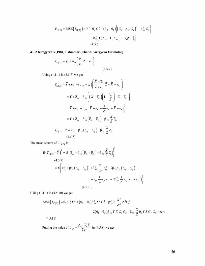
56

( ) ( )( ) ( ) ( ){ }22 2 2 22 2 112 2 11 2MSE y x xy y xy yV T Y C C C C⎡= = θ + θ − θ − ρ − ρ⎢⎣

( ){ }2 21 z xz y yz y yzC C C ⎤+θ ρ − ρ − ρ ⎥⎦

(4.5.6) 4.5.2 Kiregyera’s (1984) Estimator (Chand-Kiregyera Estimator)

( )1

2 213 21

.yxx

T y b Z xz

⎛ ⎞= + −⎜ ⎟

⎝ ⎠

(4.5.7)

Using (1.1.1) in (4.5.7) we get

( ) ( ) 1

2 21

13 2x

y yx r xz

X eT Y e e Z X e

Z e

⎛ ⎞+⎜ ⎟= + + β + − −⎜ ⎟+⎝ ⎠

( )

( )

1

2 1 2

2 1 1 2

2 1 2 1

1 zy yx x x

y yx x z x

y yx x x yx z

eY e X e X e

Z

XY e X e e X eZ

XY e e e eZ

⎛ ⎞⎛ ⎞= + + β + − − −⎜ ⎟⎜ ⎟⎜ ⎟⎜ ⎟⎝ ⎠⎝ ⎠

⎡ ⎤= + + β + − − −⎢ ⎥

⎣ ⎦

= + + β − − β

( ) ( )2 1 2 113 2 y yx x x yx zXT Y e e e eZ

− = + β − − β

(4.5.8)

The mean square of ( )13 2T is

( )( ) ( )2 1 2 1

22

13 2 y yx x x yx zXE T Y E e e e eZ

⎡ ⎤− = + β − − β⎢ ⎥

⎣ ⎦

(4.5.9)

( ) ( )2 1 2 1 2 1 2

222 2 2 22 2y yx x x yx z yx y x x

XE e e e e e e eZ

⎡= + β − + β + β −⎢

⎢⎣

( )2 1 1 1 2

22yx y z yx z x xX Xe e e e eZ Z

⎤−β − β − ⎥

⎦

(4.5.10)

Using (1.1.1) in (4.5.10) we get

( )( ) ( )2

2 2 2 2 2 2 2 22 2 1 113 2 2MSE y yx x yx z

XT C Y X C Z CZ

= θ + θ − θ β + β θ

( )1 2 12 zeroyx y x yx y zXY X C C Y Z C CZ

+ θ − θ β − β θ +

(4.5.11)

Putting the value of xy yyx

x

C YX C

ρβ = in (4.5.8) we get

57

( )( ) ( )

( )

2 2 22 2 2 2

2 1 113 2 2 2

2 2 2

1 1 22 2

1

MSE

2

xy yy x

x

xy y xy yy x xy

xx

xy yy z yz

x

C YT C Y X C

X C

C Y C YX Z Y X C CX CX C Z

C Y X Y Z C CX C Z

ρ= θ + θ − θ

ρ ρ+ θ − θ − θ ρ

ρ− θ ρ

or

( )

( )

2 22 2 2 2 2

2 2 1 1 2

2 2 22 1 12 2

y zy y xy xy

x

zxy y xy yz y

x

C CY C C

CC

C CC

⎡= θ + θ − θ ρ + θ ρ⎣

− θ − θ ρ − θ ρ ρ

or

( ){ }2

2 2 2 2 2 2 2 2 22 2 1 1 22 2z z

y y xy xy y xy y xy yz yzx

C CY C C C C C

CC

⎡ ⎤⎡ ⎤= θ + θ − θ ρ − ρ + θ ρ − ρ ρ⎢ ⎥⎢ ⎥

⎢ ⎥⎢ ⎥⎣ ⎦⎣ ⎦

( )2

2 2 2 2 2 22 1 2 1

zy y xy xy y yz y xz y

x

CY C C C C C

C

⎧ ⎫⎛ ⎞⎪ ⎪⎡ ⎤= θ − θ − θ ρ + θ ρ − ρ − ρ⎜ ⎟⎨ ⎬⎣ ⎦ ⎝ ⎠⎪ ⎪⎩ ⎭

( ) ( )( ) ( )2

2 2 22 2 1 113 2 13 2MSE z

xy xy xz yzx

CV T Y

C

⎡ ⎤⎧ ⎫⎛ ⎞⎪ ⎪⎢ ⎥= = θ − θ − θ ρ + θ ρ − ρ − ρ⎜ ⎟⎨ ⎬⎢ ⎥⎝ ⎠⎪ ⎪⎩ ⎭⎣ ⎦

(4.5.12)

4.5.3 Kiregyera’s (1984) Regression in Regression

Kiregyera (1984) also developed a regression in regression estimator i.e.

( ) ( ) ( ){ }2 1 2 114 2 yx xzT y b x x b z Z= + − + −

(4.5.13)

This may be written as

( ) ( ) ( )2 1 2 114 2 yx yx xzT y b x x b b z Z= + − + −

( ) ( )2 1 2 1y yx x x yx xz zY e e e e= + + β − + β β −

or ( ) ( )2 1 2 114 2 y yx x x yx xz zT Y e e e e− = + β − − β β

The mean square error of ( )14 2T is

( )( ) ( )2 1 2 1

22 214 2 y yx x x yx xz zE T Y E e e e e⎡ ⎤− = + β − − β β⎢ ⎥⎣ ⎦

(4.5.14)

Taking the square of R.H.S. of (4.5.14) we get

( )( ) ( ) ( )2 1 2 1 2 1 2

22 2 2 2 214 2MSE 2y yx x x yx xz z yx y x xT E e e e e e e e⎡= + β − + β β + β −⎢⎣

58

( )2 1 1 1 2

22 2yz xz y z yx xz z x xe e e e e ⎤− β β − β β − ⎦

(4.5.15)

Using (1.1.1) we get (4.5.15)

( )( ) ( )2 2 2 2 2 2 2 2 22 2 1 114 2MSE y yx x yx xz zT Y C X C B Z C= θ + β θ − θ + θ β

( )1 2 12 2 zeroxy y x xy yx xz y z yzY C X C Y C Z C+ β θ − θ ρ − β β θ ρ + (4.5.16)

Putting the value of xy yyx

x

C YX C

ρβ = and xz x

xzz

X CZ C

ρβ = we get

( )( ) ( )

( )

2 2 22 2 2 2

2 2 114 2 2 2

2 2 2 2 22 2

1 2 2 2

1 2

1

MSE

2

2

xy yy x

x

xy y xz xz

x z

xy yy x xy

x

xy y xz xy z yz

x z

C YT Y C X C

X C

Y C X CZ C

X C Z C

Y CY C X C

X C

X C X CYC Z C

Z C X C

ρ= θ + θ − θ

ρ ρ+θ

ρ+ θ − θ ρ

ρ ρ− θ ρ

( ) ( ) ( )2 2 2 2 2 22 2 1 12 2y xy xy xy xz xy xz yzY C ⎡ ⎤= θ − θ − θ ρ − ρ + θ ρ ρ − ρ ρ ρ

⎣ ⎦

or ( ) ( )( ) ( ) ( )2 2 2 2 2

2 114 2 14 2MSE 1 2y xy xy xz xy xz yzV T Y C ⎡ ⎤= = θ − ρ + θ ρ + ρ − ρ ρ ρ⎣ ⎦

(4.5.17)

4.5.4 Some Modifications of Kiregiyera’a Estimators

( ) ( )21 115 2

2xz

yT z b X x

z⎡ ⎤= + −⎣ ⎦

(4.5.18)

Using (1.1.1) in (4.5.18) we get

( ) ( ) ( )2

1 12

15 2y

z xz r xz

Y eT Z e e X X e

Z e

+⎡ ⎤= + + β + − −⎣ ⎦+

On simplification we get

( ) ( ) ( )2 1 2 115 211y z z xz xT Y e e e eZ

⎡ ⎤= + + − − β⎢ ⎥⎣ ⎦

(4.5.19) or

( ) ( )2 1 2 115 2 y z z xz xY YT Y e e e eZ Z

= + + − − β

(4.5.20)

Putting the value of yz yxz

x

ZCX C

ρβ = in (4.5.20) we get

59

( ) ( )2 1 2 115 2xz z

y z z xx

Z CYT Y e e e Y eZ Z X C

ρ− = + − −

( ) ( )2 1 2 115 2z

y z z xy xx

CY YT Y e e e eCZ Z

− = + − − ρ

(4.5.21)

The mean square error of ( )15 2T is

( )( ) ( )( ) ( )2 1 2 1

2

15 2 15 2z

y z z xz xx

CY YMSE T E T Y E e e e eCZ Z

⎡ ⎤= − = + − − ρ⎢ ⎥

⎣ ⎦ (4.5.22)

Taking the square of R.H.S. of (4.5.22) we get

( )( ) ( )2 1 2 1

22 222 2 215 2 2 2 2

zy z z xz x

x

CY YMSE T E e e e eZ X C

⎡= + − + ρ⎢

⎢⎣

( )1 1 2 2 1

2

22 2 zx z z y x xz

x

CY Ye e e e eCZZ

− − − ρ

( )1 1 2

2

22 zx z z xz

x

CY e e eCX

⎤− − ρ ⎥

⎥⎦

(4.5.23)

Using (1.1.1) in (4.5.23) we get

( )( ) ( )22 2

2 2 2 2 2 2 22 2 1 115 2 2 2 2

zy z xz x

x

CY YMSE T Y C Z C X CZ X C

= θ + θ − θ + ρ θ

( )1 2 12 2 0zy z yz y x yx xz

x

CY YY Z C C Y X C CCZ X

+ θ − θ ρ − θ ρ ρ +

(4.5.24)

On simplification we get

( )( ) ( )2 2 2 2 22 2 1 115 2 y z xz zMSE T Y C C C⎡= θ + θ − θ + θ ρ⎣

( )2 1 12 2y z yz y z xyC C C C ⎤− θ − θ ρ − θ ρ ⎦

( ) ( )2 2 22 2 1 2y z y z yzY C C C C⎡= θ + θ − θ − ρ⎣

( )2 21 2xz z y z xyC C C ⎤+θ ρ − ρ ⎦

( ) ( )( ) ( ) ( ){ }2 2 2 22 2 115 2 15 2 y z y yz y yzV MSE T Y C C C C⎡= = θ + θ − θ − ρ − ρ⎢⎣

( )1 2 2xz z y xy y xyC C C ⎤⎧ ⎫= ρ − ρ − ρ⎨ ⎬⎥⎩ ⎭⎦

(4.5.25) 4.5.5 Second Modification of Kiregyera’s Estimator

60

( )1

2 216 21

yzz

T y b X zx

⎡ ⎤= + −⎢ ⎥

⎣ ⎦

(4.5.26)

Using (1.1.1) in (4.5.26) we get

( ) ( )1

2 21

16 2z

y yz zx

Z eT Y e b X Z e

X e

⎡ ⎤+= + + − +⎢ ⎥

+⎢ ⎥⎣ ⎦

or

( ) ( ) 1

2 1 216 2 1 xy yz z z

eT Y e Z e Z e

X

⎡ ⎤⎛ ⎞− = + +β + − − −⎢ ⎥⎜ ⎟⎜ ⎟⎢ ⎥⎝ ⎠⎣ ⎦

2 1 2 1y yz z z x

Ze Z e Z e eX

⎡ ⎤= + β + − − −⎢ ⎥

⎣ ⎦

or

( ) ( )2 1 2 116 2 y yz z z xZT Y e e e eX

⎡ ⎤− = + β − −⎢ ⎥

⎣ ⎦

(4.5.27)

The mean square error of ( )16 2T is

( )( ) ( )( ) ( )2 1 2 1

22

16 2 16 2T y yz z z yz xZMSE T E Y E e e e eX

⎡ ⎤= − = + β − − β⎢ ⎥

⎣ ⎦ (4.5.28)

Taking the square of R.H.S. of (4.5.28) we get

( )( ) ( ) ( )2 1 2 1 1 1 2

222 2 2 216 2 2 2y yz z z yz x yz x z z

Z ZMSE T E e e e e e e eXX

⎡= + β − + β + β −⎢

⎢⎣

( )2 1 1 1 2

22 2yz y x yz x z zZ Ze e e e eX X

⎤− β − β − ⎥

⎦

(4.5.29)

Using (1.1.1) in (4.5.29) we get

( )( ) ( )2 2 2 2 2 2 2 2 22 2 1 116 2 y yz z yz xMSE T Y C Z C Z X C= θ + β θ − θ + β θ

( )1 2 12 2 0yz y z yz yz y z yzZY ZC C Y XC CX

− β θ − θ ρ − β θ ρ − (4.5.30)

Putting the value of yz yyz

z

Y CZ C

ββ = in (4.5.30) we get

( )( ) ( )

( )

2 2 2 2 2 22 2 2 2 2 2 2

2 2 1 116 2 2 2 2 2

1 2 12

yz y yz yy z x

z z

yz y yz yy z yz y x xy

z z

Y C Y CMSE T Y C Z C Z X C

Z C Z C

Y C YC ZY ZC C Y X C CXZ C Z C

ρ ρ= θ + θ − θ + θ

ρ ρ+ θ − θ ρ − θ ρ

On simplification we get

61

( )( ) ( )2

2 2 2 2 2 22 2 1 116 2 2

xy y yz yz y

z

CMSE T Y C C C

C

⎡= θ + θ − θ ρ + θ ρ⎢

⎢⎣

( ) 2 2 21 2 12 2 x

y yz y yz xyz

CC C

C⎤

+ θ − θ ρ − θ ρ ρ ⎥⎦

or

( )2

2 2 2 22 1 21 2x x

y yz yz yz xyzz

C CY C

CC

⎡ ⎤⎛ ⎞= θ − ρ + θ ρ − ρ ρ⎢ ⎥⎜ ⎟⎜ ⎟⎢ ⎥⎝ ⎠⎣ ⎦

or

( )2

2 2 2 2 2 22 1 21 2 2x x

y yz yz xy xy xyzz

C CY C

CC

⎡ ⎤⎛ ⎞= θ − ρ + θ ρ + ρ − ρ − ρ⎢ ⎥⎜ ⎟⎜ ⎟⎢ ⎥⎝ ⎠⎣ ⎦

or

( ) ( )( ) ( )2

2 2 2 22 116 2 16 2 1 x

y yz yz xy xyz

CV MSE T Y C

C

⎡ ⎤⎧ ⎫⎛ ⎞⎪ ⎪⎢ ⎥= = θ − ρ + θ ρ − ρ − ρ⎨ ⎬⎜ ⎟⎢ ⎥⎝ ⎠⎪ ⎪⎩ ⎭⎣ ⎦ (4.5.31)

4.6 Sahoo et al Estimator

The following estimators will be considered

a) ( ) ( ) ( )2 1 2 117 2 yx yzT y b x x b Z z⎡ ⎤= + − + −⎣ ⎦

b) ( ) ( ) ( )2 1 2 118 2 yz yxT y b z z b x X⎡ ⎤= + − + −⎣ ⎦

4.6.1 Sahoo et al (1993)

Sahoo et al (1993) developed another type of regression estimator i.e.

( ) ( ) ( )2 1 2 117 2 yx yzT y b x x b Z z= + − + −

(4.6.1)

Using (1.1.1) in (4.6.1) we get

( ) ( ) ( ) ( ) ( )2 1 2 118 2 y yx r x x yz r zT Y e e e e e e= + + β + − + β + −

( )2 1 2 1y yx x x yz zY e e e e= + + β − − β

or ( ) ( )2 1 2 117 2 y yx x x yz zT y e e e e− = + β − − β

(4.6.2)

The mean square of ( )17 2T

( )( ) ( )( ) ( )2 1 2 1

2 2

17 2 17 2 y yx x x yz zMSE T E T Y E e B e e e⎡ ⎤= − = + − − β⎣ ⎦

(4.6.3)

Taking the square of R.H.S. of (4.6.3) we get

( ) ( )2 1 2 1 2 1 2

22 2 2 2 2y yx x x yz z yx y x xE e e e e e e e⎡= + β − + β + β −⎢⎣

62

( )2 1 1 1 22 2yz y z yx z x xe e e e e ⎤− β − β − ⎦

(4.6.4)

Using (1.1.1) in (4.6.4) we get

( )( ) ( )2 2 2 2 2 2 22 2 1 117 2MSE y yx x yz zT Y C X C Z C= θ + θ − θ β + θ β

( )1 2 12 2 0yx y x xy yz y z yzY C X C Y C ZC+ β θ − θ ρ − θ β ρ + (4.6.5)

Putting the value of yxβ and yzβ in (4.6.5) we get

( )( ) ( )

( )

2 2 22 2 2 2

2 2 117 2 2 2

2 2 22 2

1 1 22 2

1

MSE

2

2

xy yy x

x

yz y xy yz y x xy

xz

yz yy z yz

z

Y CT Y C X C

X C

Y C YCZ C Y C X C

X CZ C

Y CY C Z C

Z C

ρ= θ + θ − θ

ρ ρ+θ + θ − θ ρ

ρ− θ ρ

or ( )( ) ( )2 2 2 2 2

2 2 1 1 117 2 y xy xy yzMSE T Y C ⎡ ⎤= θ + θ − θ ρ + θ ρ − θ ρ⎣ ⎦

or ( ) ( )( ) ( ) ( )2 2 2 2 2

2 117 2 11 2MSE 1y xy xy yzV T Y C ⎡ ⎤= = θ − ρ + θ ρ − ρ⎣ ⎦

(4.6.6)

63

4.6.2 Modification of Sahoo et al Estimator

( ) ( ) ( ){ }2 1 2 118 2 yz zxT y b z z b x X= + − − −

(4.6.7)

( ) ( ) ( )2 1 2 118 2 yz yz zxT y b z z b b x X= + − − − ,

(4.6.8)

where yzb is sample estimate from second phase and zxb sample estimate from the first phase. Using (1.1.1) in (4.6.8) we get

( ) ( ) ( )2 1 218 2 y yz r z zT Y e e Z e Ze= + β + + − ( )( ) ( )1yz r zx r xe e X e X′− β + β + + −

or on simplification

( ) ( )2 1 2 118 2 y yz z z yz zx xT Y e e e e− = β − − β β

(4.6.9)

The mean square error of ( )18 2T is

( )( ) ( )( ) ( )2 1 2 1

2 2

18 2 18 2 y yz z z yz zx xMSE T E T Y E e e e e⎡ ⎤= − = + β − − β β⎣ ⎦ (4.6.10)

Squaring the R.H.S. of (4.6.10) we get

( )( ) ( ) ( )2 1 2 1 2 1 2

22 2 2 2 218 2 2y yz z z yz zx x yz y z zMSE T E e e e e e e e⎡= + β − + β β + β −⎢⎣

( )2 1 1 1 2

22 2yz zx y x yz zx x z ze e e e e ⎤− β β − β β − ⎥⎦

(4.6.11)

Using (1.1.1) in (4.6.11) we get

( )( ) ( )2 2 2 2 2 2 2 2 22 2 1 118 2 y yz z yz xz xMSE T Y C Z C X C= θ + θ − θ β β β θ

( )1 2 12 0yz y z yz yz xz y x xyY ZC C X YC C+β θ − θ ρ − β β θ ρ + (4.6.12)

Putting the value of andyz zxβ β in (4.6.12)

( )( ) ( )2 2 2 2 2 2

2 2 2 2 2 22 2 1 118 2 2 2

yz y xz zy z x

z z

Y C Z CMSE T Y C Z C X C

Z C ZC

ρ ρ= θ + θ − θ + θ

12 2yz y yz y xy zy z yz y x xy

z z x

YC YC ZCY ZC C Y XC C

ZC ZC XC

ρ ρ ρ+ ρ − θ ρ

(4.6.13)

on simplification we get

( )( ) ( )

( )

2 2 2 2 2 2 2 22 2 1 118 2

2 2 2 2 21 2 12

y yz y yz y

y yz y yz xz xy

MSE T Y C Y C Y C

C Y C Y

= θ + θ − θ ρ + θ ρ

+ θ − θ ρ − θ ρ ρ ρ

or ( )( ) ( ) ( ) ( )2 2 2 2 2 2

2 2 1 1 2 118 2 2 2y yz yz yz xz yz xz xyMSE T C Y ⎡ ⎤= θ + θ − θ ρ + θ − θ ρ + θ ρ ρ − ρ ρ ρ⎣ ⎦

64

( )( ) ( ) ( )2 2 2 2 22 2 1 118 2 2y yz yz xz yz xz xyMSE T C Y ⎡ ⎤= θ − θ − θ ρ + θ ρ ρ − ρ ρ ρ⎣ ⎦

( ) ( )( ) ( ) ( )22 2 22 118 2 18 2 1y yz yz xz yzV MSE T C Y ⎡ ⎤= = θ − − ρ + θ ρ ρ − ρ⎢ ⎥⎣ ⎦

(4.6.14)

4.7 Roy’s (2003) Unbiased Regression Estimator

Roy (2003) proposed an unbiased estimator. He has used partial information.

( ) ( ){ } ( ){ }2 1 1 2 1 2 3 219 2T y k x k Z z x k Z z⎡ ⎤= + + − − + −⎢ ⎥⎣ ⎦

(4.7.1)

( ) ( )

( ) ( ) ( )2 1 1 1 2 1 2 1 3 2

2 1 1 2 1 2 1 1 3 2

y k x k k Z z k x k k Z z

y k x x k k Z z k k Z z

= + + − − − −

= + − + − − −

( ) ( ) ( )2 1 2 1 2y x x Z z Z z= + α − + β − + γ − (4.7.2)

1 1 2 1 3where k k k k kα = β = γ = −

( ) ( ) ( ) ( )2 1 2 1 219 2 y x x z zT Y e e e Z Z e Z Z e= + + α − + β − − + γ − −

( )2 1 2 1 2y x x z zY e e e e e+ + α − −β − γ

( ) ( )2 1 2 1 219 2 y x x z zT Y e e e e e− = + α − − β − γ

MSE of ( )19 2T is

( )( ) ( )2 1 2 1 2

2 2

19 2 y x x z zE T Y E e e e e e⎡ ⎤− = + α − − β − γ⎣ ⎦

(4.7.3)

We want to get the optimum value of , andα β γ for this we differentiate w.r.t. α

( ) ( ) ( )

( )2 1 2 1 2 1 1 2

2 1 2

2y x x x x z x x

z x x

E e e e e e e e e

e e e

⎡= − + α − − β −⎢⎣⎤−α − ⎦

( ) ( )

( ) ( )

2 22 1 1 2

1 20 0y x xy x

z x xz

Y X C C X C

Z X C C

= θ − θ ρ + α θ − θ

−β −γ θ − θ ρ =

( ) ( )

( )

2 22 1 1 2

1 2 0y x xy x

z x xz

Y X C C X C

Z X C C

= θ − θ ρ + α θ − θ

−γ θ − θ ρ =

2 2x z x xz y x xyX C Z X C C Y X C Cα − γ ρ = ρ

( )1 2 0x z xz y xyX C Z C Y C⎡ ⎤θ − θ α − γ ρ − ρ =⎣ ⎦

(4.7.3)

Now differentiate w.r.t. β

( )2 1 1 1 2 1 1 2

2 0y z z x x z z zE e e e e e e e e⎡ ⎤+ − − β − γ =⎣ ⎦

65

2 2 2 2

2 2 2

2 2 2

0

0y z yz z z

y yz z z

Y Z C C Z C Z C

Y C Z C Z C

θ ρ − θ β − θ α =

θ ρ − θ β − θ γ =

2 0z z y yzB Z C Z C Y C⎡ ⎤θ + γ − ρ =⎣ ⎦

(4.7.4)

Now differentiate w.r.t. γ

( )( )( )( )

2 2 2 1 2 1 2 2

2

2 2 2 2 22 2 1 1 2

2 2 1 1 2

0

0

0

y z z x x z z z

y z yz z x xz z z

y yz x xz z z

E e e e e e e e e

Y Z C C Z X C C Z C Z C

Y Z C X C Z C Z C

+ α − − β − γ =

θ ρ + α θ − θ ρ − βθ − γ θ =

⇒ θ ρ + α θ − θ ρ − θ β − γ θ =

( )2 2 1 1 2 0z y yz z zZ C Y C Z C Z Cγ θ − θ ρ + θ β + θ − θ α =

( ) ( )2 1 1 2 0z y yz z zZ C Y C Z C Z Cθ γ − ρ + θ β + θ − θ α =

(4.7.5)