hands on training 8 measurement of loudspeaker directivity · loudspeaker under test and the...

KLIPPEL E-learning, training 8 2018-12-19

1

Hands-On Training 8

Measurement of Loudspeaker Directivity

1. Objective of the Hands-on Training

- Understanding the need for assessing loudspeaker directivity

- Introducing the basic theory of acoustic holography and field separation

- Applying Near Field Scanning techniques to loudspeakers

- Interpreting the results of Near Field Scanning

- Developing skills for performing practical measurements

2. Requirements

2.1. Previous Knowledge of the Participants

It is recommended to do the Klippel Training #2 “Vibration and Radiation Behavior of

Loudspeaker’s Membrane” before starting this training.

2.2. Minimum Requirements

The objectives of the hands-on training can be accomplished by using the results of the

measurement provided in a Klippel database (.kdbx) dispensing with a complete setup of the

KLIPPEL measurement hardware. The data may be viewed by downloading the measurement

software dB-Lab from www.klippel.de/training and installing them on a Windows PC.

2.3. Optional Requirements

If the participants have access to a KLIPPEL Analyzer System, we recommend to perform

some additional measurements on loudspeakers provided by instructor or by the participants.

In order to perform these measurements, you will also need the following additional software

and hardware components:

Klippel Robotics

KLIPPEL Analyzer (DA2 or KA3)

Near Field Scanner

Amplifier

Microphone

3. The Training Process

Read the following theory to refresh your knowledge required for the training.

Watch the demo video to learn about the practical aspects of the measurement.

Answer the preparatory questions to check your understanding.

Follow the instructions to interpret the results in the database and answer the multiple-

choice questions off-line.

Check your knowledge by submitting your responses to the anonymous evaluation

system at www.klippel.de/training.

Receive an email containing a Certificate with high distinction, distinction or credit

(depending on your performance).

Perform some optional measurements on transducers if the hardware is available.


2

4. Introduction

Nowadays, there is an increasing demand for better quality of the reproduced sound in home

entertainment, virtual reality, mobile, automotive, professional and other applications. This

training focuses on the direct sound radiated by the audio device into the 3D space into

different directions (angles) and distances (near and far field). This part gives a short

introduction of the theoretical basis and the practical methods required to measure the sound

pressure distribution as shown in the Figure 4.1.

At low frequencies the driver can be simulated by using a lumped parameter model. The

electrical stimulus (voltage 𝑢 and current 𝑖) at the terminals generates the electro-dynamical

force 𝐹coil . This force drives the mechanical elements represented by moving mass 𝑀ms , stiffness of the suspension system 𝐾ms and mechanical resistance 𝑅ms and generates the voice

coil velocity 𝑣coil . An electrical stimulus (voltage 𝑢) and a mechanical signal (velocity 𝑣)

describe the transfer of an audio signal in a one dimensional signal path to the diaphragm

(Training 1).

At higher frequencies, a model comprising a multitude of distributed parameters and state

variables is required to describe the modal vibration of the diaphragm and suspension system

(Training 2).

VibrationMotor Radiation Near

FieldFar

Field

Voice

Coil

Radiator�s

Surface

)( cv r

)( cF rcoilF

coilv

u

i )( np r )( ap r

Terminals

Distributed Parameters

Electrical

Measurement

Mechanical

Measurement

Far Field

Response

Vibration,

Geometry

Lumped Parameters

TS

Parameter Near Field

Response

Acoustical

Measurement

Figure 4.1 Measurement Process of Loudspeakers [1]

The velocity 𝑣(𝑟c) in the normal direction at any point 𝑟c on the radiating surface generates the

sound pressure values 𝑝(𝑟n) and 𝑝(𝑟a) in the near field and far field respectively. This tutorial

focuses on the acoustical measurement in near field and far field, as shown in the Figure 4.1.

4.1. Direct Sound Radiated by the Loudspeaker

Sound is an oscillation of the medium (e.g. air) that generates variation in the pressure

propagating as waves away from its source. The speed of sound c depends on the static air

pressure, density (or humidity and temperature) of the medium. The sound pressure, which is

the difference between the instantaneous value of the total pressure and the static pressure, is

much easier to measure than density or temperature fluctuations [3]. An important

characteristic is the sound pressure level, denoted by 𝐿𝑝 or SPL and defined by:

𝐿𝑝 = 20log10 (𝑝

𝑝0) dB

(1)

with the reference pressure 𝑝0 = 20μPa.


3

The homogeneous wave equation (2) describes the relationship between temporal and local

derivative of the sound pressure in a medium [4].

∆ 𝑝 =1

𝑐2𝜕2𝑝

𝜕𝑡2

(2)

According to equation (2) the sound wave is propagated into different directions with the

speed of sound c.

At low frequencies, a closed box loudspeaker system can be approximated by a point source

(monopole) that generates spherical waves under free field condition that fulfil the one-

dimensional wave equation in spherical coordinates:

𝜕2(𝑝𝑟)

𝜕𝑟2=1

𝑐2𝜕2(𝑝𝑟)

𝜕𝑡2

(3)

The product of distance 𝑟 and pressure 𝑝 in Equation (3) propagates with the speed of sound c

away from the sound source. Thus, the amplitude of the sound pressure decays inversely with

distance 𝑟:

|𝑝(𝑟)| ∝1

𝑟

(4)

4.2. Far-field Conditions

This so called 1/𝑟-law is also valid for a vented-box loudspeaker system or any other sound

source with an arbitrary shape if the observation point is in the far field of the source where

the distance 𝑟 is larger than a critical value 𝑟far . This critical value 𝑟far depends on the

wavelength 𝜆 of a sinusoidal sound component and the largest geometrical dimension l of the

sound source:

lr

Condition 1: 𝑟far

𝑙≫ 1 (5)

r

λ


𝜆≫ 1 (6)

lr

λ


𝑙≫

𝑙

𝜆 (7)

Figure 4.2 Far Field Conditions

Condition 1 requires that the size of loudspeaker is small compared to the distance 𝑟 .

Condition 2 requires that the distance is larger than the wavelength which is a critical

condition at low frequencies. Condition 3 is a critical condition for large loudspeaker systems

used at the high frequencies such as line arrays, sound bars and panels. [8]


4

For a typical loudspeaker as used in home application the linear relationship (1/𝑟 -law)

between sound pressure 𝑝 and distance 𝑟 begins at distance 𝑟 > 2 m. At closer distance, the

sound pressure 𝑝 rises at a much higher slope due to the near field properties generated by the

size of the diaphragm and the number of transducers used in the system.

nref

orefϕ

θ

r

Figure 4.3 Coordinate System

If the complex sound pressure 𝑃(𝑓, 𝑟1, 𝜃, 𝜙) is given at distance 𝑟1 in the direction represented

by polar angle 𝜃 and azimuthal angle 𝜙, the sound pressure at a different distance 𝑟2 can be

calculated by

)(

2

112

12),,,(),,,(rrjk

er

rrfPrfP

(8)

using the wave number 𝑘 = 2𝜋𝑓/c. In the far field the sound pressure 𝑝 and particle velocity 𝑣 are in phase and the specific sound

impedance is a real value 𝑍𝑎 ≈ 𝜌c. There is no reactive component [6] and the sound power

𝛱 propagated by the sound wave can be calculated as the integral over the intensity 𝐼 = 𝑝𝑣

over the spherical surface 𝐴 as follows:

𝛱 = ∮𝑝𝜈 d𝐴 (9)

The Sound Power Level, denoted by 𝐿𝛱, is given in decibel (dB) by:

𝐿𝛱 = 10log10(𝑃

𝑃ref𝑊)

(10)

using the reference value 𝑃ref = 10−12𝑊.

The sound radiation behavior is defined under free field conditions where the influence of the

sound reflections, diffraction and standing waves caused by boundaries (e.g. room walls) does

not exist.


5

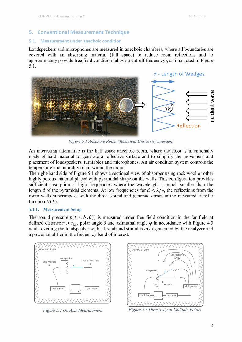
5. Conventional Measurement Technique

5.1. Measurement under anechoic condition

Loudspeakers and microphones are measured in anechoic chambers, where all boundaries are

covered with an absorbing material (full space) to reduce room reflections and to

approximately provide free field condition (above a cut-off frequency), as illustrated in Figure

5.1.

Inci

den

t w

ave

d - Length of Wedges

Reflection

Figure 5.1 Anechoic Room (Technical University Dresden)

An interesting alternative is the half space anechoic room, where the floor is intentionally

made of hard material to generate a reflective surface and to simplify the movement and

placement of loudspeakers, turntables and microphones. An air condition system controls the

temperature and humidity of air within the room.

The right-hand side of Figure 5.1 shows a sectional view of absorber using rock wool or other

highly porous material placed with pyramidal shape on the walls. This configuration provides

sufficient absorption at high frequencies where the wavelength is much smaller than the

length 𝑑 of the pyramidal elements. At low frequencies for 𝑑 < 𝜆/4, the reflections from the

room walls superimpose with the direct sound and generate errors in the measured transfer

function 𝐻(𝑓).

5.1.1. Measurement Setup

The sound pressure 𝑝(𝑡, 𝑟, 𝜙 , 𝜃)) is measured under free field condition in the far field at

defined distance 𝑟 > 𝑟far, polar angle 𝜃 and azimuthal angle 𝜙 in accordance with Figure 4.3

while exciting the loudspeaker with a broadband stimulus 𝑢(𝑡) generated by the analyzer and

a power amplifier in the frequency band of interest.

r

Anechoic Room

AnalyzerAmplifier

Sound Pressurep

Loudspeaker

Input Voltageu

Figure 5.2 On Axis Measurement

Anechoic Room

AnalyzerAmplifier

Turntable

r

Multiplexer

Microphone Array

Loudspeaker

Figure 5.3 Directivity at Multiple Points


6

Figure 5.2 shows the measurement setup of assessing the radiated sound pressure

𝑝(𝑡, 𝑟, 𝜃 = 0°) at the reference axis (also called “On-Axis response”) to describe the sound

pressure output in the direction that is most relevant for the particular application. The

loudspeaker under test and the microphone are placed at a fixed position. Figure 5.3 depicts

the multi-point measurement using a turntable or other robotics for turning the loudspeaker

around polar angle 𝜃 or azimuthal angle 𝜙 while using a microphone array for measuring the

sound pressure versus the orthogonal angle. The spacing of the microphones and the

increments of the turntable movements determine the number of measurement points and the

angular resolution of the directivity data. The measurement over the complete sphere (4π)

requires a compromise between the angular resolution and the number of measurement points:

Angular

resolution over the

complete sphere (4π)

Number of

measurement

points

5 degree 2592

2 degree 16200

1 degree 64800

Most conventional measurements provide no higher angular resolution than 2 degree and

assume symmetry in one or two-planes to reduce the measurement time.

5.1.2. Directional Transfer Function

This chapter gives an overview on the post-processing to calculate the linear transfer function

from the loudspeaker input voltage 𝑢(𝑡) to the sound pressure output 𝑝(𝑡, 𝑟, 𝜙, 𝜃) at the

microphone position.

KLIPPEL

-130

-120

-110

-100

-90

-80

-70

-60

-50

-40

-30

1 2 5 10 20 50 100 200 500 1k 2k 5k 10k 20k

Voltage Spectrum at TerminalsVoltage Speaker 1

dB - [V]

(rms)

Frequency [Hz]

Signal lines Noise floor

Noise floor

Voltage spectrum

Complex transfer function

FT

KLIPPEL

55

60

65

70

75

80

85

90

95

50 100 200 500 1k 2k 5k 10k

Magnitude of transfer function H(f)

dB - [V

/ V]

Frequency [Hz]

Magnitude

Magnitude response

KLIPPEL

-150

-100

-50

0

50

100

150

50 100 200 500 1k 2k 5k 10k

Phase of transfer function H(f)

[deg]

Frequency [Hz]

Phase

Phase response

Distance > 1 m

KLIPPEL

-1,0

-0,5

0,0

0,5

1,0

0 250 500 750 1000 1250

Stimulus (t) vs time

[V]

Time [ms]

Stimulus (t)

Shaped Stimulus

KLIPPEL

-20

-10

0

10

20

30

40

50

60

70

80

5 10 20 50 100 200 500 1k 2k 5k 10k 20k

Sound Pressure spectrumSignal at IN2

dB - [V]

(rms)

Frequency [Hz]

Signal lines Noise floor

Noise floor

Sound pressure spectrum

KLIPPEL

-300

-200

-100

0

100

200

300

400

500

600

0 1 2 3 4 5 6 7 8

Impulse response h(t)

[V / V]

left:0.875 Time [ms] right:4.958

Measured Windowed

Impulse

responsewindow w(t)

� 𝑡, 𝑟, , = −1𝑃( , 𝑟, , )

( )

= 𝐹 𝑢(𝑡) 𝑃 , 𝑟, , = 𝐹 𝑝(𝑡, 𝑟, , )

𝐻 , 𝑟, , = � 𝑡, 𝑟, , (𝑡)

Figure 5.4 Overview on the Calculation of the Complex Transfer Function [10]

The first step is the calculation of the complex spectrum (jω)of the input signal 𝑢(𝑡) generated by the analyzer and the sound pressure spectrum 𝑃(jω, 𝑟, 𝜙, 𝜃)measured by the

microphone. Sufficient signal to noise ratio (SNR) is required to measure the transfer function


7

accuracy. Figure 5.4 shows an example of insufficient SNR in the sound pressure signal for

frequencies below 30 Hz. The SNR can be improved by applying higher amplitude shaping to

the stimulus at low frequencies. Alternatively, averaging of the measured sound pressure

signal can be applied if a deterministic stimulus such as a sinusoidal chirp is used.

The second step is the calculation of the impulse response �(𝑡, 𝑟, 𝜙, 𝜃) defined as

�(𝑡, 𝑟 𝜙, 𝜃) = −1 {𝑃(j , 𝑟, 𝜙, 𝜃)

(j )}

(11)

based on the inverse Fourier transform applied to the ratio of complex output and input

spectra. A window function (𝑡) may be applied to the impulse response �(𝑡, 𝑟, , 𝜃) in order

to separate the direct sound from room reflections and to suppress measurement noise. The

Fourier transform applied to the windowed impulse response gives the directional transfer

function:

𝐻(j , 𝑟, 𝜙, 𝜃) = {�(𝑡, 𝑟, 𝜙, 𝜃) (𝑡)} (12)

75

80

85

90

95

100

105

110

115

120

20 50 100 200 500 1k 2k 5k 10k 20k

Frequency [Hz]

-1400

-1200

-1000

-800

-600

-400

-200

0

200

400

600

-20 0 20 40 60 80 100

Impulse response

[V / V

]

Time [ms]

Direct Sound

Direct Sound

smoothed by time window

Measured Sound(disturbed by reflections)

First Reflections

Reflectionszero padding

Tw

fw=1/Tw

Transfer function

Figure 5.5 Windowing of the Impulse Response

Figure 5.5 illustrates time windowing of the impulse response �(𝑡, 𝑟, 𝜙, 𝜃) to suppress room

reflections while preserving the direct sound at higher frequencies 𝑓 > 𝑓w. This critical cut-

frequency 𝑓w = 1/ w depends on the effective length w of the time window (𝑡) . The

window in Figure 5.5 has a flat top region generating an effective window length w = 7 ms

and reduces the true spectral resolution. At low frequencies below 𝑓w = 150 Hz the

measurement points in the frequency response are generated by zero padding and are not real

measurement data.

dms

Reflective Surface

dsr dr

MicrophoneSpeaker

Figure 5.6 Sound Reflected on the nearest Boundary

Distance of first reflection:

𝑑r = 2√(1

2𝑑ms)

2

+ (𝑑sr)2

(13)

𝑑𝑚𝑠 distance microphone to speaker

𝑑𝑠𝑟 distance speaker to room wall

The maximum length of window w should be shorter than reflection free time max defined

as:


8

𝑤 < max =𝑑r− 𝑑

ms

𝑐

(14)

5.2. Directional Far-Field Characteristics

The term directivity has been introduced to describe the distribution of the direct sound on a

sphere depending on the polar angle 𝜃 and azimuthal angle 𝜙 at a particular distance 𝑟 in far

field.

5.2.1. Directional Factor and Gain

The ratio between the complex sound pressure value 𝑃(𝑓, 𝑟, 𝜃, 𝜙) at any azimuthal angle 𝜙

and polar angle 𝜃 to the sound pressure value 𝑃(𝑓, 𝑟, 𝜃𝑟 , 𝜙𝑟) defined by reference angles 𝜙𝑟 and 𝜃𝑟measured in the far-field of the DUT gives the directional factor

𝛤(𝑓, 𝜃, 𝜙) =𝑃(𝑓, 𝑟, 𝜃, 𝜙)

𝑃(𝑓, 𝑟, 𝜃𝑟 , 𝜙𝑟)=𝐻(𝑓, 𝑟, 𝜃, 𝜙)

𝐻(𝑓, 𝑟, 𝜃𝑟 , 𝜙𝑟)

(15)

And the directional gain in dB

,,log20),,( ffD (16)

In most applications the reference angles 𝜙𝑟 = 0° and 𝜃𝑟 = 0° describe the on-axis response

measured on the reference axis perpendicular to the diaphragm of the loudspeaker. [17]

Theta in Degree

Reference Axis

10dB

Figure 5.7 Polar plot

-180

-160

-140

-120

-100

-80

-60

-40

-20

0

20

40

60

80

100

120

140

160

180

100 1k 10k

Th

eta

in D

egre

e

f in Hz

Reference Axis

Figure 5.8 Contour plot

The directional gain is useful to visualize the beaming of the loudspeaker and the decay of the

sound pressure level versus angle 𝜃 as a polar, contour or balloon plot.

5.2.2. Directivity Factor and Index

By integrating the squared directional factor over the unit sphere the directivity factor Q(f)

can be calculated as

𝑄(𝑓) =4𝜋

∫ |𝛤(𝑓,𝜃,𝜙)|2 dΩΩ

(17)

giving the directivity index in dB:

𝐷𝐼(𝑓) = 10log10 𝑄(𝑓) (18)

A loudspeaker operated in a sealed box has a directivity index DI ≈ 0 dB at low frequencies,

which corresponds to an omnidirectional radiation pattern generating the same sound pressure

level at the same distance r for any polar angle θ and azimuthal angle ϕ. At higher

frequencies, the loudspeaker generates a lower sound pressure on the rear side than on the

front side which increases the directivity index.


9

5.3. Limitations of the Far Field Measurements

The precision of the far field measurement setup depends on the following conditions:

1. Defined microphone placement

2. Defined positioning of the DUT (while turning heavy devices)

3. Sound reflection from turntable

4. Early reflections on room walls

5. Temporal and local variation of air properties (temperature, humidity) versus the

propagation path affect the phase response (2° Kelvin deviation generates 90° phase

error in 5 m distance at 5 kHz)

6. Air convection (wind)

7. Influence of ambient noise

8. Sufficient angular resolution

An anechoic room usually provides good wind protection and sufficient suppression of

ambient noise. However, room modes can generate 1-6 dB errors at low frequencies and the

temperature can cause significant phase errors at high frequencies. Furthermore, the

conventional measurement technique cannot check those requirements and detect errors

automatically. Since there is usually no redundancy in the measured data set, it is difficult to

identify faulty measurements and exclude those points from the post-processing.

Figure 5.9 5° Angular Resolution

Figure 5.10 1° Angular Resolution

Interpolation of the phase and amplitude between the measurement points will introduce a

significant error if the angular resolution in the measurements cannot cope with directional

complexity of the loudspeaker. For example, the polar plot shown in Figure 5.9 measured

with 5° angular resolution cannot represent the narrow lobes coming up in the measurement

with 1° resolution as shown in Figure 5.10. Some of the peaks and dips in the polar plot are

completely missed.


10

6. Near Field Measurement

6.1. Motivation

There are multiple reasons why measurements in the near field are relevant and beneficial

although the simple extrapolation based on the 1/r-law is not applicable in general.

The near field properties of the DUT determine the sound pressure at the listener’s ear

in studio monitors, laptops, tablets, smart-phones and other portable audio devices.

Sound bars, professional line arrays and other large loudspeakers have to be measured

in the near field, because the far field distance rfar cannot be realized in available

anechoic rooms.

The measurement in the near field provides a good signal-to-noise ratio, which

reduces the influence of ambient noise, the generation of nonlinear distortion and

dispenses from excessive averaging (time saving).

The amplitude of direct sound is much greater than room reflections. The direct sound

arrives much earlier at the microphone than the first reflections from room boundaries.

This provides good conditions for simulating free field conditions by gating

techniques or windowing of the impulse response.

There is only a minimal influence from air properties.

6.2. Holographic Near Field Measurement

The holographic near field measurement exploits the general three-dimensional wave

equation (2) expressed in spherical coordinates as given in [15]. The solution of this equation

can be described by a spherical wave expansion

),()()(

),()()(),,,(

)1(

0

,

)2(

0

,

m

nn

N

n

n

nm

in

mn

m

nn

N

n

n

nm

out

mn

Ykrhjc

YkrhjcrjP

(19)

which is valid in the region where no boundaries and sound sources are found as shown in

Figure 6.1.

region of validity

surface

sound source

external sound source

(ambient noise)

external boundaries

(walls)

+ ),,,( rp

Figure 6.1 Spherical wave expansion

The first expansion term containing the Hankel function of the second kind hn(2)

(kr) represents

the outgoing waves. The second term containing the Hankel function of the first kind hn(1)

(kr)


11

represents the incoming waves. The Hankel functions describe the dependency of the radial

coordinate r. For large distances r > rfar the absolute value of the Hankel functions of any

order n decay inversely with r corresponding with the 1/r-law. The spherical harmonics

Ynm(θ,) found on both terms describe the dependency on azimuthal angle and polar angle θ.

Monopole

Dipoles

Quadrupoles

Figure 6.2 Spherical harmonics (real parts)

The spherical harmonic 𝑌𝑛𝑚(𝜃, 𝜙) = 1/√4π represents a monopole with an omnidirectional

radiation behavior as shown in Figure 6.2. The first order spherical harmonics 𝑌1−1(𝜃, 𝜙),

𝑌10(𝜃, 𝜙) and 𝑌1

1(𝜃, 𝜙), can be used to represent angular directivity of a dipole with any

orientation in the spherical coordinate system. The spherical harmonics are orthonormal and

provide a complete set of basic functions for the spherical wave expansion with the Hankel

function of order n.

The coefficients 𝑐𝑛,𝑚𝑜𝑢𝑡( ) and 𝑐𝑛,𝑚

𝑖𝑛 ( ) weight each basic function and may be interpreted as

the spherical wave spectrum analogically to the coefficients of the Fourier series.

+q

-q

Woofer

Port

Dipole

Figure 6.3 Spherical Wave Expansion of a Vented-Box System below port resonance

For example, a vented-box system as shown in Figure 6.3 behaves below the port resonance

like a dipole where the port and the diaphragm generate the same amplitude but opposite sign

of the volume velocity q. The polar plot of the directional gain would generate two lobes in

opposite direction separated by a null that is perpendicular to the line between the two

monopoles. If the port and woofer are placed in the z-axis with polar angle θ = 0°, the

spherical harmonic 𝑌10(𝜃, 𝜙) corresponds to the directivity of the vented box system and a

single coefficient 𝑐1,0𝑜𝑢𝑡( ) represents the radiation behavior.

This example shows that the maximum order N of the wave expansion and the number of

coefficients depend on

the directional complexity of the loudspeaker under test, which rises usually with

frequency

the location of the expansion point (origin of the internal coordinate system) in the

acoustical center

the orientation of the loudspeaker in the spherical coordinate system.


12

6.3. Directional Transfer Function

The directional transfer function of the loudspeaker between input voltage u(t) and sound

pressure output p(t) at the measurement point r under free field condition, can be expressed by

considering only the direct sound pDir(t) in Equation (19):

𝐻(j , 𝑟, 𝜃, 𝜙) =𝑃𝑝Dir(j , 𝑟,θ, 𝜙)

(j )= ∑ ∑ 𝐶𝑚𝑛(j )

𝑛

𝑚=−𝑛

𝑁

𝑛=0

�𝑛(2)(𝑘𝑟)𝑌𝑛

𝑚(𝜃, 𝜙) (20)

Grid CalculationRobotics +

Measurement

Transformation of coordinates

Optimal Parameter Fitting

TESTINGFitting Error

Post processing

Order of expansion

Symmetry Detection

Expansion point detection

Visualization

User Input

][iG

)(rp

)( Ep r

)( fC

Q

EPr

N

),( Efe r

Figure 6.4 Practical measurement procedure

6.4. Practical Measurement Procedure

Figure 6.4 illustrates the measurement procedure which comprises the following steps:

1. The device under test (loudspeaker) is placed on the robotics as shown in Figure 6.5.

2. The microphone is moved manually to the upper corner of the device under test and to

the tweeter to measure important geometrical information which are used for

calculating the initial scanning grid G[i=0]. The scanning grid contains measurement

points distributed on an inner and an outer surface which is a requirement to separate

the incoming and outgoing sound waves (field separation) at lower frequencies.

3. The measurement determines the transfer function between the input signal u(t) and

the sound pressure p(t,r) at any point r on the scanning grid G[i].

4. The holographic processing starts with the transformation of the data p(t,r) in the

measured coordinates into an internal coordinates system p(t,rE) that has its origin

close to the acoustical center for high frequencies (tweeter position) and the

coordinates are aligned to the orientation of the speaker.

5. The coefficients 𝑐𝑛,𝑚𝑜𝑢𝑡( ) and 𝑐𝑛,𝑚

𝑖𝑛 ( ) in Equation (19) are estimated by minimizing

the mean squared error e(f) between the modelled and measured sound pressure on the

scanning grid.

6. The final coefficients Cmn(jω) in Equation (20) representing the direct sound radiated

by the loudspeaker are calculated based on the field separation technique.


13

7. In an optional iteration additional measurement points can be acquired based on the

position of the expansion point rEP to improve the angular resolution and the maximum

order of the expansion N.

8. The sound pressure level or the directional transfer function 𝐻(j , 𝑟, 𝜃, 𝜙) can be

calculated at any measurement point outside the outer scanning surface. Post-

processing provides additional characteristics such as directional gain, directivity

index and sound power.

Microphone

Phi-Axis

Z-AxisR-Axis

Figure 6.5 Near Field Scanner

6.5. Checking the Accuracy of the Measurement

The accuracy of the directional transfer function can be easily checked by assessing the fitting

error

𝑒(𝑓) =∑ |𝐻(𝑓, 𝒓) − 𝐻meas(𝑓, 𝒓)|

2

∑ |𝐻meas(𝑓, 𝒓)|2∙ 100% (21)

that compares the modeled response H(f,r) and the measured response Hmeas(f,r) at all

measurement points r on the scanning grid G[i].

The calculation of the error e(f) requires that there is some redundancy in the measured data

set, that means the number M of measurement points is larger than the number of unknown

coefficients in the wave expansion J.

𝑀 ≥ 𝐽 = (𝑁 + 1)2 (22)

The error may be caused by the following factors:

Maximum order N of the wave expansion is too low to describe the directional

complexity of the loudspeaker

Ambient noise or a poor signal-to-noise ratio (SNR) of the microphone corrupt the

measured data

The position of the loudspeaker or the microphone have been changed during the

scanning process


14

KLIPPEL

-60

-55

-50

-45

-40

-35

-30

-25

-20

-15

-10

-5

0

5

100 1k 10kf in Hz

-20dB= 1%

N=0

N=1

N=2

N=3

N=5

N=10

Noise Floor

Figure 6.6 Fitting Error as a function of the maximum order of the expansion N

For example, Figure 6.6 shows the fitting error versus frequency for the wave expansion with

varying maximum order N. The closed-box loudspeaker system cannot be described with

sufficient accuracy by using a single monopole (N = 0). Considering a monopole together

with dipoles (N = 1) reduces the error between 50 Hz and 500 Hz to -10 dB. Increasing the

maximum order N = 2 and considering quadrupoles the error can be reduced to -20 dB. This

means that only 1 % of the radiated power cannot be explained by the model. Above 500 Hz

the loudspeaker starts beaming and additional side lobes increase the directional complexity

that require a maximum order of N > 10 to reduce the fitting error below -20 dB at 10 kHz.

Increasing the order N will not reduce the fitting error below 30 Hz because the error is

caused by ambient noise. The grey dashed line shows a relative sound pressure level

measured with no excitation signal on the loudspeaker under test.

50

55

60

65

70

75

80

85

90

95

100

105

110

100 1k 10k

Sou

nd

Po

wer

in d

B

f in Hz

n=0

n=1

n=2

n=3

Total Radiated Power

Figure 6.7 Sound Power contributed by spherical waves


15

Figure 6.7 shows the contribution of the spherical waves of order n to the total sound power

radiated from the loudspeaker under test into the far field. At 70 Hz the monopole (n = 0)

dominates the total power which corresponds to the closed-box design and the fact that the

wavelength is much larger than the geometrical dimension of the diaphragm and the box.

However, the dipole (n = 1) provides ~20 dB less power, which can be explained by the fact

that the acoustical center of a sealed box system is about 5 cm in front of the diaphragm of the

woofer and not identical with the origin of the wave expansion which is placed close to the

tweeter. The quadrupoles (n = 2) are ~40 dB lower but rising rapidly with frequency and

exceed the monopole at ~1 kHz. While the higher-order waves (n > 5) provide a small

contribution below 5 kHz they come more and more important at higher frequencies.

-50

0

50

100

150

200

250

300

0.1m 1m 10mDistance

Monopole

Far FieldNear Field

Order n of the Spherical Waves

Sou

nd

Po

wer

in d

B

n=0n=3n=5

n=7

n=10n=9n=8

Figure 6.8 Apparent Sound Power versus Distance r

Figure 6.8 shows the apparent sound power of the nth

-order waves versus the distance r at

1 kHz. The apparent power describes also the near field (r < 1 m) where the sound pressure

and velocity are not in phase. There the apparent power is inversely related to the distance r

corresponding to the nth

-order Hankel functions hn(2)

(kr) and hn(1)

(kr) in Equation (19). At high

order n the apparent power rises with high slope to significant values which are much higher

than real power radiated into the far field.

The estimated values between the surface of the loudspeaker enclosure and the scanning area

(0.2 m < r < 0.4 m) are less accurate than the extrapolated values outside the scanning

surface. The values that are predicted inside the loudspeaker system (r < 0.2 m) have to be

considered as virtual values generated by wave expansion neglecting any boundary and have

no practical value.

The apparent power becomes constant for a distance r > rfar which is at 1 kHz approximately

1 m. Here, the apparent power becomes identical with real power propagated into the far field

because pressure and particle velocity are in phase. At this frequency the wave expansion

truncated after N = 5 can sufficiently describe the radiation of the loudspeaker while the other

higher-order waves (n > 5) propagate negligible power.

6.6. Field Separation

Windowing of the impulse response according to Equation (12) is a simple and reliable

method to separate the direct sound from the room reflections at high frequencies. The

effective window length Tw, limited by reflection free time Tmax as defined by Equation (14),

provides sufficient resolution to capture the direct sound at high frequencies and is usually to

short measure the direct sound with sufficient resolution at low frequencies.


16

65707580859095

100105110115

100 1k 10kf in Hz

SPL

in d

B

Measured Sound

Direct Sound

Room Reflections

Ref

lect

ion

Fre

e F

req

uen

cy

Field Separation by Holographic Processing

Field Separation by Time Windowing

Figure 6.9 Results of the sound separation

The wave expansion according to Equation (19) provides an alternative to separate direct

sound from the room reflections at low frequencies. This method requires a low order

(N < 10) of spherical harmonics due to the large wavelength in this frequency band

(f < 3 kHz). Figure 6.9 shows the amplitude response of a loudspeaker system between the

input and the total sound pressure measured at a particular microphone position. This curve

reveals peaks and dips in the amplitude response below 500 Hz which are caused by the

interferences of room modes and early reflections. The sound separation provides the

amplitude response of the direct sound that corresponds with the expected theoretical

behavior. The second term in Eq. (19) comprising the coefficient scaling the Hankel function

hn(1)

(kr) represents the incoming sound generated by the sound reflections at the room

boundaries. Figure 6.9 also shows the generated amplitude response of this incoming sound

part with peaks and dips at particular frequencies which depend on the size and shape of the

room, the acoustical properties of the reflecting surfaces and the position of the speaker and

microphone. If the level difference between the direct sound and the room reflections is small,

the measured sound will be affected. The holographic wave separation is not required at

higher frequencies ( f > 3 kHz) where the time windowing of the impulse response can be

applied.


17

7. Preparatory Questions

Check your theoretical knowledge before you start the regular training. Answer the questions

by selecting all correct responses (sometimes, there will be more than one).

QUESTION 1: Why is the measurement of the directivity important for assessing loudspeakers?

(section 4)

□ MC a: The directivity of the loudspeaker describes the amplitude and phase of direct sound

radiated into a particular direction.

□ MC b: The directivity of the loudspeaker describes the properties of the loudspeaker which

are important to model the interactions with the acoustical environment such as early

and late room reflections and standing waves.

□ MC c: The directivity of the loudspeaker describes the maximum output of the loudspeaker

limited by transducer nonlinearities and thermal overload.

QUESTION 2: What are the differences between far field and near field of a complex sound source?

(section 4)

□ MC a: The sound pressure and particle velocity are in phase in the far field.

□ MC b: The total sound power will not change with the distance r from the source in far

field.

□ MC c: The total sound power will decay by 6 dB per octave for doubling the distance r in

far field.

□ MC d: The sound power in the near field has a reactive component.

□ MC e: The sound power in the far field has a reactive component.

QUESTION 3: How to ensure far field measurement conditions? (section 4.2)

□ MC a: Distance r between sound source and measurement point should be larger than the

largest dimension l of the radiating surface.

□ MC b: Distance r is smaller than the largest dimension l of the radiating surface.

□ MC c: Distance r is larger than the wavelength λ of the lowest spectral component

measured.

□ MC d: Distance r is smaller than the wavelength λ of the lowest spectral component

measured.

□ MC e: The ratio r/l between distance r and geometrical dimension l should be larger than

the ratio l/λ between geometrical dimension l and wavelength λ.

□ MC f: The distance r should be large enough to ensure that the sound pressure is 6 dB

lower than in the near field of the source.

QUESTION 4: Does the 1/r-law depend on frequency? (section 4.2)

□ MC a: Only high frequency components decrease inversely with distance r in far field (with

r > rfar).

□ MC b: All frequency components decrease inversely with distance r in far field (with

r > rfar).

□ MC c: The critical distance rfar(f) is usually a function of frequency f.

□ MC d: The critical distance rfar is a constant which only depends on the size of the

loudspeaker but is independent of the frequency f.


18

QUESTION 5: Why is the directivity factor defined in the far field of the source? (section 5.2)

□ MC a: The directivity factor is independent of the distance r if the measurement is

performed in the far field (r > rfar).

□ MC b: The measurement of the sound pressure output is performed at a larger distance from

the source (far field condition) to avoid that ambient noise corrupts the measurement

results.

□ MC c: Any positioning error of the microphone and loudspeaker has a smaller impact on

the measured magnitude response at a larger distance (r > rfar).

□ MC d: Any positioning error of the microphone and loudspeaker has a smaller impact on

the measured phase response at a larger distance (r > rfar).

□ MC e: The measurement of the sound pressure output is performed at a larger distance from

the source (far field condition) because the direct sound can be more easily separated

from room reflections by windowing the impulse response.

QUESTION 6: Why is an anechoic room beneficial for loudspeaker measurements? (section 5.1)

□ MC a: Air movement (wind) can be avoided.

□ MC b: Inhomogeneous temperature distribution can be reduced by using an air condition

system.

□ MC c: The microphone can be placed very close to the loudspeaker while maintaining far-

field conditions.

□ MC d: External ambient noise can be reduced by using thick walls and a floating

foundation.

□ MC e: A full space anechoic rooms provides perfect free field conditions.

QUESTION 7: Are loudspeaker measurements affected by standing wave (modes) and sound

reflections in an anechoic room? (section 5.1)

□ MC a: Yes, the absorbing material placed on the walls cannot damp the sound reflections at

low frequencies, which may affect the sound pressure response measured in the far

field of the loudspeaker.

□ MC b: No, if all reflecting boundaries are covered with absorbing material (the thickness is

not critical) the measurement room will have perfect anechoic properties.

□ MC c: If the microphone is placed in the near field of the loudspeaker, close to the

diaphragm and the distance to the walls is significantly large, than the reflective

sound may be negligible compared to the direct sound.

QUESTION 8: Why are characteristics that describe the near field properties important for assessing

audio devices? (section 6.1)

□ MC a: The near field properties of studio monitors are relevant for sound engineer who

have their listening position close to the speakers.

□ MC b: Laptops, tablets, PC multi-media audio, smart phones and other personal audio

equipment are used in the near field.

□ MC c: The near field properties reveal the dominant nonlinearities inherent in the

loudspeakers.


19

QUESTION 9: Under which condition can the far field characteristics of a loudspeaker be derived

from near field data? (section 6.2)

□ MC a: When the loudspeaker is a transducer that is mounted in a sealed enclosure, it

generates an omnidirectional radiation characteristic (monopole) at low frequencies.

In this case, the 1/r-law is valid for the far field and also for the near field.

□ MC b: The sound pressure in the near field has to be scanned at multiple points on a

scanning surface around the loudspeaker with sufficient angular resolution. The

measured sound pressure data is modelled by superposition of scaled basic functions

that are the solution of the wave equation and describe the propagation of sound into

the far field (holographic measurement).

□ MC c: Valid far field data can be calculated from near field measurements by windowing

the impulse response.

□ MC d: Accurate far field data can only be derived from a single sound pressure

measurement if the microphone is located in the acoustical center of the source.

QUESTION 10: What affects the angular resolution of the measured directivity determined by near

field scanning technique and holographic wave expansion? (section 0)

□ MC a: The angular density of the scanning grid, corresponding to the number and

placement of the measurement points, determines the angular resolution of the

measured directivity.

□ MC b: The holographic processing performs an angular interpolation between the measured

samples based on the basic functions that fulfil the wave equation. Thus the angular

resolution of the measured directivity may be higher than the angular density of the

measurement points on the scanning surface. This interpolation is only correct if the

order of the wave expansion is high enough to describe the sound field at the

investigated frequency without aliasing.

□ MC c: The maximum order N of the wave expansion determines the angular resolution of

measured directivity.

□ MC d: The orientation of the loudspeaker during the scanning process determines the

angular resolution of the measured directivity data.

QUESTION 11: What are the results of the holographic measurement? (section 0)

□ MC a: The frequency response of the complex coefficients 𝑐𝑛,𝑚𝑜𝑢𝑡( ) weighting the spherical

harmonics Ynm(θ,) and Hankel function hn

(2)(kr).

□ MC b: The amplitude and phase of the directional transfer function 𝐻(j , 𝑟, 𝜃, 𝜙) describing the relationship between loudspeaker input voltage and sound pressure of

the outgoing wave at a point in the far field.

□ MC c: The basic functions such as the spherical harmonics Ynm(θ,) and the Hankel

functions.

□ MC d: The total sound pressure and the sound pressure generated by an outgoing wave at

any point r in the 3D space outside the scanning surface.

□ MC e: The total sound pressure extrapolated at any point r in the 3D space between

loudspeaker surface and the scanning surface.


20

QUESTION 12: Why is the extrapolation of the sound pressure to an observation point in the far field

possible based on a wave expansion measured in the near field? (section 6.2)

□ MC a: The extrapolation is possible, because the Hankel functions hn(1)

(kr) describe the

relationship between sound pressure versus distance r for an incoming wave.

□ MC b: Spherical harmonics Ynm(θ,) describe the sound pressure versus distance r.

□ MC c: The basic function, which is composed of Hankel function hn(2)

(kr) and spherical

harmonics Ynm(θ,), tells the relationship between sound pressure versus distance and

angles for outgoing waves.

□ MC d: There are no additional sound sources and boundaries in the space between the

scanning surface in the near field and observation point in the far field.

QUESTION 13: How can the accuracy of the holographic measurement results be checked? (section

6.5)

□ MC a: The sound pressure is scanned at multiple layers where measurement points are

located at similar direction (φ1 ≈ φ2, θ1 ≈ θ2) but at different distances (r1 ≠ r2)

from the source. The holographic processing calculates the fitting error between

measured and modelled sound pressure and uses the redundancy in the input data to

evaluate the discrepancy in the modelling.

□ MC b: The measurement is repeated by using the identical scanning process (position and

number of the measurement points) and the agreement between the two independent

holographic measurements is evaluated.

□ MC c: The standard deviation of the sound pressure is calculated over all measurement

points and compared with the permissible threshold.

QUESTION 14: Does a very low fitting error ensure an accurate measurement? (section 6.5)

□ MC a: Yes, a low fitting error means the constructed sound pattern perfectly matches the

real sound pattern

□ MC b: No, a good fitting error means that the measured data agrees with the modeled data.

If the position and orientation of the loudspeaker is not well defined or has been

changed during the scanning process the measured data will be misinterpreted and

have no practical value.

□ MC c: No, if all measurement points are placed on a single scanning surface there is no

redundancy of the data versus distance r and the measurement noise will be

interpreted as directional information. Therefore, measurement on to interlaced

scanning surfaces is useful for checking the accuracy of the measurement even if

separation of incoming and outgoing waves is not required in this frequency range.

QUESTION 15: Which are the theoretical reasons for an unacceptable fitting error? (section 6.5)

□ MC a: The maximum order N of expansion is not high enough to model the sound field

generated by the loudspeaker.

□ MC b: Ambient noise corrupts the measured data.

□ MC c: The loudspeaker generates plane or cylindrical waves which cannot be fitted by

spherical waves.


21

QUESTION 16: How can the direct sound be separated from room reflections? (section 6.6)

□ MC a: Applying windowing to the measured impulse response, extracting the first part of

the impulse response which corresponds to the direct sound and attenuating the late

part of the impulse response which corresponds to the room reflections.

□ MC b: Scanning the sound pressure on two interlaced surfaces around the sound source and

performing an expansion of the measured sound pressure in outgoing and incoming

sound waves.

□ MC c: Scanning the sound pressure on a single surface around the sound source and

performing a holographic processing of the data.

QUESTION 17: What are the benefits of using a holographic scanner in an anechoic room? (section

0)

□ MC a: The ambient noise caused by external sound sources (e.g. traffic, production noise)

can be reduced.

□ MC b: The measurement time can be reduced by skipping a double scan required for sound

separation, because the room influence at low frequencies can be neglected in the

near field where the direct sound is dominant.

□ MC c: Multiple holographic scanning systems can only be operated in an anechoic room.

QUESTION 18: Which restrictions affect the separation of direct sound and room reflections at high

frequencies by windowing the impulse response? (section 0)

□ MC a: The loudspeaker should be placed in the middle of the room to generate the

maximum distance to the room boundaries that gives the largest time difference

between the direct sound radiated by the loudspeaker and the room reflections

arriving at the loudspeaker diaphragm. The position of the microphone is not critical.

□ MC b: The microphone should be placed in the middle of the room to generate the

maximum distance to the room boundaries and the largest delay of the room

reflections. The position of the loudspeaker is not critical.

□ MC c: The distance dms between the microphone and speaker and the minimum distance dsr

between the speaker and the room boundaries (walls, ceiling, ground) determines the

reflection free time Tmax between first arrival of the direct sound and room

reflections. This time Tmax determines the width Tw of the window and the spectral

resolution Δf = 1/Tw of the measured transfer function.

QUESTION 19: How can the number of measurement points in the scanning process be reduced

while maintaining sufficient angular resolution and accuracy? (section 6.4)

□ MC a: The maximum order N of the expansion can be reduced if the fitting error does not

exceed a critical limit (-20 dB) in the frequency range of interest.

□ MC b: The scan can be performed on a single layer if the transfer function is assessed at

higher frequencies where the sound separation can be performed by windowing of

the impulse response.

□ MC c: Improving the signal to noise ratio of the measurement by increasing the amplitude

of the stimulus.


22

QUESTION 20: How can the direct sound be separated from the room reflections? (section 6.4)

□ MC a: Holographic field separation can be applied to the sound pressure measured on two

interlaced scanning surfaces with different distance r1 ≠ r2 from the expansion point.

□ MC b: Holographic field separation cannot be used at low frequencies where the

wavelength is larger than the size of the device under test.

□ MC c: Windowing of the impulse response can be used to suppress the room reflections at

high frequencies where the reflection free time Tmax is larger than the window length

Tw = 1/Δf providing the requested frequency resolution Δf.

□ MC d: Windowing of the impulse response can be used to separate the direct sound at low

frequencies where the reflection free time Tmax is much smaller than the window

length Tw = 1/Δf providing the requested frequency resolution Δf.

□ MC e: Windowing of the impulse response requires scanning of the sound pressure on two

interlaced scanning surfaces with different distance r1 ≠ r2 from the expansion

point.

QUESTION 21: Which of the following statements about time windowing are correct? (sections 0

and 0)

□ MC a: Time windowing can be used for the entire frequency range to separate incoming

and outgoing waves.

□ MC b: Time windowing is used for the high frequency range because it saves time and is

easy to implement.

□ MC c: Windowing of the impulse response will not affect the spectral resolution of the

transfer function at low frequencies if the truncated impulse response is extended by

zero padding before applying the FFT giving a high spectral resolution.

□ MC d: The measurement of the sound pressure on one scanning surface is sufficient to

separate the direct sound from the room reflections by time windowing.

QUESTION 22: Why does the near field scanner move the microphone, but keep the sound source at

the fixed position? (section 0)

□ MC a: A turntable cannot be used for moving the loudspeaker, because the holographic

processing requires scanning data which correspond to a constant interaction

between loudspeaker and acoustical boundaries (e.g. walls).

□ MC b: Moving heavy loudspeakers at high accuracy puts high demands on the positioning

system. A microphone can be moved at a higher speed, higher accuracy and at lower

cost.

□ MC c: Traditional techniques cause artefacts in the measured transfer function due to sound

reflections at the turntables while the near field scanning minimizes those errors by

placing the device under test on a small post. All other parts of the robotics are

outside the scanning surface and can be separated by sound separation.

□ MC d: To minimize the cost of the 3D scanner required for measuring the sound field

generated by the loudspeaker in three dimensions (spherical coordinates). There are

no acoustical reasons for moving the microphone.


23

8. Interpretation of measurement results (no hardware required)

Step 1: View the demo video Measurement of Loudspeaker Directivity provided at

www.klippel.de/training/ to see the practical measurement of loudspeakers

Step 2: Install the KLIPPEL R&D software dB-Lab on your computer and download

the database corresponding to this training.

Step 3: Start dB-Lab by clicking on the file <>

Advice: It is recommended to do the following exercises offline and to note the answers

of the multiple choice questions on a paper!

Basic Sound Transmission

In dB-Lab, firstly open the folder NFS Tutorial. And then open the object 1. Near Field vs.

Far Field. Double click on Device Introduction (line array) to see the line array loudspeaker

in the coordinate system. Double click the 4 objects 1a to 1d that are showing polar plots

measured at different distances r = 2, 4, 8 and 16 m.

QUESTION 23: Watch and compare the 4 polar plots at 4.9 kHz and explain the differences.

□ MC a: The graphs in red (ϕ = 0°) showing the vertical sound pattern are much more

beaming to the reference axis (θ = 0) and has much more side lobes than the blue

horizontal pattern (ϕ = 90°).

□ MC b: The graphs in red (ϕ = 0°) showing the vertical sound pattern changes significantly

with increasing distance r while the blue horizontal pattern (ϕ = 90°) is almost

constant.

□ MC c: Multiple transducers placed vertically in the line array generate a significant near

field effect.

□ MC d: The far field of this loudspeaker starts at a distance of 4 meter.

Double click on the object 1e. SPL decay (1/r Law), which is showing the difference of the

SPL responses when doubling the distance.

QUESTION 24: Which of the following statements are correct?

□ MC a: The measurement at low frequencies (f < 1 kHz) is already performed under far field

condition for a distance r ≥ 2 meters, because the SPL decreases by approximately

6 dB per doubling the distance.

□ MC b: All the measurements are not performed under far field condition, because the SPL

decreases not by approximately 3 dB for doubling the distance r.

□ MC c: The mismatch of the SPL difference per doubling the distance to the 1/r-law at high

frequencies is caused by external noise during the measurement.

□ MC d: The mismatch of the SPL difference per doubling the distance to the 1/r-law at high

frequencies is caused by the near field effect.

http://www.klippel.de/training/


24

QUESTION 25: Which is the most important far field condition for the line array operated at high

frequencies?

□ MC a: Condition 1: 𝑟far

𝑙≫ 1, the far field begins when the distance is much larger than the

size of the box.

□ MC b: Condition 2: 𝑟far

𝜆≫ 1, the far field begins when the distance is much larger than the

wavelength.

□ MC c: Condition 3: 𝑟far

𝑙≫

𝑙

𝜆, the far field starts when the

𝑟far

𝑙2 is much larger than the

reciprocal of the wavelength.

Now open the object 2. Room Mode showing the measurement on a two-way speaker using a

vented box system and horn compression driver. View the operations 2a. Near field SPL

front side and 2b. Near field SPL rear side, which show the SPL response at same distance

on-axis at front and rear side of the loudspeaker. The red curve labeled Measured shows the

SPL directly measured by the microphone. The blue curve labeled Radiated shows the direct

sound separated from the room reflections (dashed blue curve) by the field separation

technology.

QUESTION 26: Explain the difference of the SPL response at the rear and front side of the

loudspeaker?

□ MC a: The wave length is large at low-frequencies (f < 1 kHz) and the radiated sound is less

influenced by diffraction at the loudspeaker box.

□ MC b: Voice coil inductance increases the electrical input impedance at higher frequencies

and reduces the input current, displacement and radiated sound pressure.

□ MC c: With rising frequency the wave length becomes shorter and the geometry of the

loudspeaker box reduces the sound pressure level on the rear side.

Select the curve Room Reflections in the window Near Field SPL Response in operation 2b,

copy this curve into the clip board (by using right mouse button) and paste this graph in the

corresponding window of 2a. Compare the SPL representing the room reflections on the rear

and back side of the loudspeaker.

QUESTION 27: Why are the fluctuations in the SPL measured at the rear side (2b) much stronger

than in the SPL measured at the front?

□ MC a: The room reflections approaching the rear side of the loudspeaker are much stronger

than the room reflections approaching the front side.

□ MC b: The room reflections have almost the same SPL at the rear and front side. But the

room reflections have a much higher impact on the measured response on the rear

side because the direct sound (fitted) radiated by the loudspeaker has a much lower

SPL there.

□ MC c: The SNR is much lower at the rear side than that at the front side.


25

Loudspeaker Analysis

Open the object 3. Sound Power & On-axis SPL response showing the measurement results

of a studio monitor.

Inspect the window Far Field SPL Response in operation 3a On-axis SPL and Power

response that shows the SPL (red curve) at 10 m distance on axis and the Radiated Sound

Power (dashed green curve) at a reduced level (-30 dB). Compare the shape of the two curves.

QUESTION 28: Why is the Sound Power response decreasing significantly above 200 Hz while the

SPL Response on the reference axis (θ = 0°) stays approximately constant?

□ MC a: The loudspeaker starts becomes more directional at higher frequencies and starts

beaming to the front side. Since the active loudspeaker system is equalized to an

approximately constant on-axis response, the sound power decreases at high

frequencies.

□ MC b: The loudspeaker behaves at high frequency like a monopole.

□ MC c: The sound power increases to lower frequencies because the loudspeaker is more

directional at low frequencies.

The holographic measurement of a line array, sound bar or other loudspeaker system using

multiple transducers, a wave expansion with a large maximum order N > 30 and a large

number of measurement points J > 1000 are required to fit the sound pressure in the near field

at sufficient accuracy. An interesting alternative is the superposition principle where each

transducer in the loudspeaker system is measured separately and the total system is modeled

by the superposition of the sound fields generated by each transducer.

Optionally, a linear control system can be applied to each transducer for beam shaping and

steering the directivity pattern. This approach requires less measurement points than the

holographic measurement of the sound field generated by the complete loudspeaker system.

Open the object 4. Crossover that shows further measurements on the Studio monitor which

uses a tweeter and a woofer in a two-way configuration with a crossover at 2.1 kHz. The

window Far field SPL response in the first operation 4a shows the SPL response of the

complete two-way system where woofer and tweeter are excited by the stimulus. The

operation 4b shows the SPL responses of the woofer and tweeter where two independent

scans where only one transducer is excited during each scanning process. The red curve

shows total SPL response calculated by adding the complex transfer functions of the woofer

and tweeter.

The operation 4c shows the difference between the SPL response measured on the total

system and the SPL response calculated by the superposition of the tweeter and woofer

measurements.

QUESTION 29: Which benefits brings the superposition of SPL measured by multiple scans?

□ MC a: The scanning grid can be optimized according to the position of the transducer

excited during the individual test. This reduces the number of measurement points

required to fit the measured sound field by the wave expansion.

□ MC b: The origin of coordinate system used in the spherical wave expansion can be placed

in the acoustical center of the particular transducer excited during each scanning

process. The coordinates of the individual expansion points shall be considered in

the superposition of the sound fields.

□ MC c: Performing multiple scans improves the signal to noise ratio because the multiple

SPL curves are added.


26

Open the object 6. Angular Resolution and inspect the results of a near field scanning (6a)

and a conventional far field measurement (6b) applied to the same line array. The operation

6a (NFS) shows the extrapolated SPL in the far field (r = 10 m) as a polar plot in the

horizontal plane (ϕ = 90°) and vertical plane (ϕ = 0°) with 180° < θ < 180° based on 2500

measurement points placed close to the speaker. The operation 6b. Polar plots (conventional)

shows the result of the direct measurement of the SPL in the far field (r = 10 m) using a

turntable with 5 degree increments over the azimuthal and polar angles generating

approximately the same number of measurement points as used in the near field scanning.

Compare the vertical polar plot (ϕ = 0°) shown as red graph with -180° < θ < 180° in the

operations 6a and 6b.

QUESTION 30: What causes the difference between the vertical polar plots (red graphs) provided by

the two measurements?

□ MC a: The polar plot provided by the near field scanner (NFS) provides a much higher

angular resolution than the density of the measurement points on the scanning grid,

because the polar pattern is reconstructed between the measured points on the grid

by using the solution of the wave equation.

□ MC b: The polar plot provided by the conventional far field measurements provides an

angular resolution which is identical with the angular increments of the measurement

points generated by the turntables.

□ MC c: The higher complexity of the curve shape in the polar plot generated by the near

field scanner is influenced by background noise.

Compare the horizontal polar plot (ϕ = 90°) shown as blue graph in the two measurements 6a

(NFS) and 6b (conventional).

QUESTION 31: What causes the lower complexity of the blue curves in the horizontal polar plot

(ϕ = 90°)?

□ MC a: The angular resolution provided by both measurement techniques (NFS and

conventional) is too small to represent the horizontal directivity.

□ MC b: The blue graph shows the horizontal polar plot of the loudspeaker, which is not

complex in directivity, because all tweeters used in the loudspeaker are placed on

line rectangular to the horizontal plane. A smaller number of measurement points

generating less angular resolution would be sufficient to represent the directivity in

this plane.

□ MC c: The horizontal directivity of the complete line array corresponds approximately with

the horizontal directivity of each tweeter used in the line array. Thus, the directional

properties of a single tweeter determine the horizontal directivity of the line array.


27

Basic Loudspeaker Knowledge

Select the object 7. Driver in vented or sealed box or in free air and view the operation 7.

Device Introduction where a woofer in free air and mounted in a vented Demo-box is shown.

The port of the Demo-box can be sealed by a plug to generate a sealed box. Each device is

measured by near field scanning and the results are presented in the following operations:

View the operation 7a. Sound Power Comparison and inspect the three diagrams showing the

far field SPL response on axis in 10 m distance, directivity index and the radiated sound

power. Compare the curves of Far Field SPL Response (10m front ON-Axis) of Vented,

Sealed, and Driver in free air.

QUESTION 32: Why does the Driver in free air (green curve) generate a much lower SPL response

at low frequencies than the driver mounted in a vented and sealed enclosure?

□ MC a: Acoustic cancellation takes place between the volume velocity generated on the

front and rear side of the driver in free air that reduces the SPL in the far field.

□ MC b: The driver operated in free air generates less cone displacement because there is no

additional stiffness provided by the air in the box. The lower displacement generates

also a lower SPL in the far field.

Inspect Far Field SPL Response (10m front ON-Axis) of the three devices at approximately

150 Hz.

QUESTION 33: Why does the vented box loudspeaker system generate a peak in the SPL frequency

response at 150 Hz which is not found in the sealed box system?

□ MC a: There is a standing wave in the sealed enclosure which increases the acoustical

impedance at this frequency and reduces the acoustical output.

□ MC b: The air mass in the port and the acoustical compliance of the air in the box build up a

resonator which increases the acoustical output at the port resonance.

□ MC c: This peak is caused by a room mode increasing the sound pressure at the microphone

position.

Inspect the diagram Directivity Index and compare the curves of the three devices at low

frequencies.

QUESTION 34: Why does the driver in free air generate a larger directivity index than the driver

operated in an enclosure?

□ MC a: At low frequencies, the driver can be regarded as a dipole, so it is more directional

than a monopole.

□ MC b: At low frequencies, the driver in free air can be regarded as a monopole, so the

directivity is higher.

□ MC c: At low frequencies, the driver in free air can be regarded as a quadrupole, so the

directivity is higher.


28

Inspect the diagram Radiated Sound Power and compare the curves of the three devices

below 50 Hz.

QUESTION 35: Why does the driver in the sealed enclosure radiate more sound power than the

driver in the vented enclosure?

□ MC a: The acoustic cancellation between the volume velocities generated by the diaphragm

and the port reduces the sound power. Therefore, the SPL frequency response

decreases with a higher slope to lower frequencies than at the sealed box.

□ MC b: The enclosed air in the sealed box provides additional acoustical stiffness which

increases the resonance frequency. A higher resonance frequency generates more

acoustical output at low frequencies.

Inspect the operations 7b-7g showing a balloon plot and the total sound power and

contribution of order N for the driver in free air, mounted in the sealed and vented enclosure.

QUESTION 36: Which spherical wave generates the largest contribution to the total sound power at

200 Hz?

□ MC a: Driver in free air: The spherical waves of order N = 1 (dipoles) radiated by the driver

in free air generate the dominant contribution.

□ MC b: Sealed box: The spherical wave of order N = 0 (monopole) radiated by the driver

mounted in a sealed enclosure generates the dominant contribution.

□ MC c: Vented box: The wave of order N = 0 (monopole) radiated by the vented box system

generates the dominant contribution.

□ MC d: Vented box: The vented box system behaves as a dipole at low frequencies. Thus, the

spherical wave of order N = 1 generated by a dipoles provides the dominant

contribution to the total power in the far field.

Field Identification

Select the object 8. Maximum Expansion Order showing the NFS measurement applied to a

Studio Monitor. Inspect the following operations 8a-8d showing the fitting error as a function

of the maximum order N with N 1, 5, 10 and 14.

QUESTION 37: What is the optimal value for the maximum order N used in the wave expansion if

the sound radiation shall be measured over the full audio band (20 Hz … 20 kHz)?

□ MC a: The maximum order of the expansion should be larger than order 14 because the

fitting error exceeds -20 dB at low frequencies.

□ MC b: The maximum order of the expansion shall be set to N = 14 because this is a good

comprise between a low fitting error (E < -20 dB) and number M of measurement

points on the scanning grid to ensure that all unknown parameters in the wave

expansion can be identified. The error below 50 Hz corresponds to the poor SNR due

to the low SPL generated by the loudspeaker. The rising fitting error corresponds to

the rising noise floor shown as a dashed grey curve in the diagram.

□ MC c: The maximum order of the expansion shall be set to N = 5 because the fitting error E

is smaller than -20 dB over a wide frequency band but increases at low and high

frequencies due to the poor SNR shown as the dashed curve in the diagram.


29

Open object 9. Time Windowing&Frequency Resolution and the operation 9a. TRF transfer

function (off-axis). Inspect the result window Impulse Response. The grey curve shows the

original impulse response h(t) and the red curve shows the impulse weighted by a half-Turkey

window w(t) between the black cursors. You can zoom in the graph by dragging with the

mouse, and undo the zoom by typing Z.

QUESTION 38: When does the first room reflection arrive at the measurement point?

□ MC a: 1.1 ms after the direct sound

□ MC b: 10.4 ms after the direct sound

□ MC c: 15.7 ms after the direct sound

Move the cursors limiting the left and right side of the window and inspect the influence on

the graph Magnitude of transfer function H(f) at low frequencies.

QUESTION 39: Where is the optimum window position?

□ MC a: The time window should be as small as possible in order to separate the direct sound

completely from the room reflections.

□ MC b: To ensure sufficient resolution at low frequencies the time window should be as

large as possible.

□ MC c: The left cursor of a half window (there is no attenuation on the left window side)

should be at the maximum of the impulse reponse.

□ MC d: The left cursor of a half window should be just before the direct sound starts and the

right cursor should provide sufficient attenuation of the first room reflections while

maximizing the length of the time window to provide maximum frequency

resolution.

A simulated free field response can also be generated by holographic field separation of the

sound pressure data that are measured on two interlaced scanning surfaces in a non-anechoic

environment.

Open the object 10. Field Separation and inspect the results of the measurements 10a with

Field Separation and 10b without Field Separation applied to a two-way loudspeaker.

Compare the diagrams Fitting Error and Near Field SPL Response of the two

measurements.

QUESTION 40: What causes the differences in the Fitting Error and Near Field SPL Response

below 2.3 kHz?

□ MC a: The fitting error is significantly reduced by considering the incoming and outgoing

waves.

□ MC b: The residual error which cannot be explained by field separation is close to the noise

floor.

□ MC c: The direct sound shown as blue solid curve (Radiated) is much smoother at low

frequencies than the total sound pressure response (Measured) and corresponds to

the theoretical behavior of a vented box system.

□ MC d: The room reflections shown as the blue dashed curve reveals the influence of the

standing waves in the room. The peaks of the room reflections correspond to the

peaks in the fitting error of the wave expansion without field separation.

□ MC e: The field separation technique uses a larger number of measurement points which

improves the signal-to-noise ratio SNR in the averaged data set.

QUESTION 41: Why is the field separation not used at high frequencies (above 2.3 kHz)?


30

□ MC a: A higher density of measurement points on the scanning grid is required to model the

room modes and sound reflections at higher frequencies. The shorter wavelength and

the discrepancy between the shape of the wave-front of the room modes

(approaching plane waves after propagation over some distance) and the spherical

waves used in the model requires a significantly larger maximum order N in the

wave expansion.

□ MC b: Windowing is a simple and reliable alternative to separate the direct sound from

room modes and sound reflections at high frequencies.

□ MC c: Field separation technique assumes that the loudspeaker under test has an

omnidirectional behavior (directivity index ≈ 0) but most loudspeakers starts

beaming at high frequencies.

Trouble Shootings

Open the object 11. TroubleShooting 1. And inspect the operations 11a and 11b, showing two

Field Identification operations based on the same scanning data, but using a different

maximum order of the expansion N.

QUESTION 42: Which operation uses a better setup for performing a fast and accurate NFS

measurement?

□ MC a: Operation 11b provides more accurate results, because the fitting error stays over a

wide frequency range below -20 dB. The fitting error in operation 11a rises with the

frequency f and exceeds the limit -20 dB at 7 kHz.

□ MC b: Operation 11a uses a smaller maximum order N = 5 of the expansion and requires

less measurement points than the setup used in operation 11b. If the device under test

is a subwoofer, where only the measurement data below 1 kHz are required, this

setup would provide sufficient accuracy in a shorter measurement time.

□ MC c: Both setups are good enough for most applications because the fitting error is not a

critical characteristic to evaluate holographic near field measurements.

Compare the impact of the setup on the directional characteristics shown in the operation 11c.

Comparison of the Results.

QUESTION 43: How does the maximum order N affect the directivity data?

□ MC a: The directional data and characteristics measured at low frequencies (< 1 kHz) are

almost not affected.

□ MC b: There are no major errors generated in the measured characteristics because the low

order coefficients in the wave expansion with order N < 5 are almost identical in

operation 11a and 11b. This is caused by the orthogonal basis functions used in the

wave expansion where higher order terms may be added without changing the lower

order coefficients.

□ MC c: The loudspeaker under test shows a high directivity index and a complex polar

pattern that requires a wave expansion of order N > 14 to ensure accurate data at

high frequencies.

□ MC d: The measurement is corrupted by ambient noise and the setup in operation 11a using

the maximum order N = 5 reduces the impact of the noise on the measured

directivity information.

Open the object 12. TroubleShooting 2 comprising the results of two measurements

performed on the same device under test by using the same setup (stimulus, scanning grid,


31

analysis). Inspect the operation 12a. First measurement and 12b. Second measurement and

check the reliability of the data.

QUESTION 44: Which measurement is valid and provides accurate and reliable results?

□ MC a: The first measurement 12a provides valid results in the frequency range from 40 Hz

to 10 kHz because the fitting error stays below -20 dB.

□ MC b: The second measurement is valid because the fitting error is below -20 dB at

selected frequencies.

□ MC c: The second measurement 12b provides invalid results below 1.3 kHz, because the

error exceed -20 dB.

□ MC d: Both measurements are not valid because the fitting error exceeds the limit -20 dB at

low and very high frequencies.

QUESTION 45: What are the causes of the invalid measurement?

□ MC a: The position of the loudspeaker has been changed during the scanning process due to

an improper clamping of the device under test on the platform.

□ MC b: The position of the microphone has been changed during the scanning process

because the microphone was loosely clamped.

□ MC c: The invalid measurement is affected by ambient noise which shown as increased

level of the grey dashed curve labeled Noise Floor. The reduced SNR has a strong

impact on the field separation technique that is used for frequencies below 1.3 kHz.

The poor SNR has much less impact on the separation technique based on

windowing the impulse response that is applied at higher frequencies.

Open the object 13. TroubleShooting 3 showing the results from a holographic measurement

of a two-way loudspeaker system using a woofer at low frequencies and a tweeter at high

frequencies. The data collected during scanning process have been used for different

holographic processing. The operation 13a. Expansion point tweeter shows the result of the

holographic processing where the origin of the spherical coordinate system was placed close

to the acoustical center at high frequencies which is close to the tweeter. The operation 13b.

Expansion point woofer shows the result of the holographic processing where the expansion

point was placed close to the woofer generating the acoustical center at low frequencies.

QUESTION 46: Where should the expansion point be placed?

□ MC a: The expansion point shall be placed close to the acoustical center.

□ MC b: In a two-way system, the acoustical center is a function of frequency and moves

from the woofer at low frequency to a point close to the tweeter at high frequencies.

The tweeter generates a more complex directional pattern than the woofer and

requires a higher maximum order N for reducing the fitting error at higher

frequencies. If the same expansion point shall be used for all frequencies, this point

should be placed close to the tweeter.

□ MC c: The expansion point can be placed anywhere in the space between the outer surface

of the loudspeaker (diaphragm, enclosure) and the scanning grid. A high fitting error

is generated, if the expansion point is placed virtually inside the loudspeaker

enclosure.

□ MC d: The expansion can be placed close to the woofer if the SPL frequency response is

only measured and evaluated at low frequencies where the woofer is active.


32

9. Performing a Sound Radiation Behavior Scan (Near Field Scanner needed)

If a near field scanner is available, it is highly recommended to perform a scan on a loudspeaker. This

is supposed to enhance the understanding of the features of Near Field Scanner.

9.1. Information to Near Field Scanner

The demo video Measurement of Loudspeaker Directivity gives you a direct view of the

software and analysis before you start to perform your measurements yourself.

9.2. Performing a scan

Please see the NFS User Manual for a detailed description of the near field scanner

measurement [16] .

10. Reference

[1] W. Klippel, Vibration and Radiation Behavior of Loudspeaker’s

Membrane, pp. 1–19, Mar. 2014.

[2] W. Klippel, Linear Lumped Parameter Measurement, pp. 1–19, Feb. 2013

[3] F. Jacobsen, An Elementary Introduction to Acoustics, pp. 1–64, Nov. 2011.

[4] S. W. Rienstra and A. Hirschberg, “An Introduction to Acoustics,” pp. 1–

296, Jan. 2015.

[5] Earl Geddes,GedLee LLC, “Directivity in Loudspeaker Systems,” pp. 1–

14, Jan. 2010.

[6] R. J. Baken and R. F. Orlikoff, Clinical Measurement of Speech and Voice.

Cengage Learning, 2000.

[7] F. Jacobsen, Active and reactive, conherent and incoherent sound fields,

pp. 1–15, 1988.

[8] M. Möser, Technische Akustik, pp. 1–552, Oct. 2015.

[9] J. G. Rodriguez, Anechoic room mechanism, pp. 1–131, Aug. 2011.

[10] W. Klippel, Sound Quality of Audio Systems Part 4:Sound Radiation,

Measurement and Room Interaction,” 2016, pp. 1–125.

[11] BAY SYSTEM Ltd., Building a semi-anechoic Chamber, pp. 1–7, Apr.

2004.

[12] D. B. KeeleJR., Low-Frequency Loudspeaker Assessment by Nearfield

Sound-pressure Measurement, pp. 1–9, 1974.

[13] G. Weinreich and E. B. Arnold, Method for measuring acoustic radiation

fields, pp. 1–8, Oct. 2011.

[14] C.-X. Bi, X.-Z. Chen, and J. Chen, Sound field separation technique based

on equivalent source method and its application in nearfield acoustic

holography, J. Acoust. Soc. Am., vol. 123, no. 3, pp. 1472–7, 2008.

[15] E. G. Williams, Fourier Acoustics, pp. 1–321, 1999.


33

[16] Software Manual: Near Field Scanner R&D System User’s guide, Klippel

GmbH

[17] IEC (E) 60268-21: Acoustical (Output based) Measurements, 2015

International Electrotechnical Commission

[18] IEC 62777 Ed.1: Quality Evaluation Method for the Sound Field of

Directional Loud-speaker Array, 2014 International Electrotechnical

Commission

[19] CEA-2034: Standard Method of Measurement for In-Home Loudspeakers,

, 2013 Consumer Electronics Association

hands on training 8 measurement of loudspeaker directivity · loudspeaker under test and the...

Documents