handbook of combinatorial optimization...
TRANSCRIPT

HANDBOOK OF COMBINATORIALOPTIMIZATIONSupplement Volume B
HANDBOOK OF COMBINATORIALOPTIMIZATIONSupplement Volume B
Edited by
DING-ZHU DUUniversity of Minnesota, Minneapolis, MN
PANOS M. PARDALOSUniversity of Florida, Gainesville, FL
Springer

eBook ISBN: 0-387-23830-1Print ISBN: 0-387-23829-8
Print ©2005 Springer Science + Business Media, Inc.
All rights reserved
No part of this eBook may be reproduced or transmitted in any form or by any means, electronic,mechanical, recording, or otherwise, without written consent from the Publisher
Created in the United States of America
Boston
©2005 Springer Science + Business Media, Inc.
Visit Springer's eBookstore at: http://ebooks.springerlink.comand the Springer Global Website Online at: http://www.springeronline.com
Preface
Combinatorial (or discrete) optimization is one of the most active fieldsin the interface of operations research, computer science, and applied math-ematics. Combinatorial optimization problems arise in various applications,including communications network design, VLSI design, machine vision, air-line crew scheduling, corporate planning, computer-aided design and man-ufacturing, database query design, cellular telephone frequency assignment,constraint directed reasoning, and computational biology. Furthermore,combinatorial optimization problems occur in many diverse areas such aslinear and integer programming, graph theory, artificial intelligence, andnumber theory. All these problems, when formulated mathematically as theminimization or maximization of a certain function defined on some domain,have a commonality of discreteness.
Historically, combinatorial optimization starts with linear programming.Linear programming has an entire range of important applications includingproduction planning and distribution, personnel assignment, finance, alloca-tion of economic resources, circuit simulation, and control systems. LeonidKantorovich and Tjalling Koopmans received the Nobel Prize (1975) fortheir work on the optimal allocation of resources. Two important discover-ies, the ellipsoid method (1979) and interior point approaches (1984) bothprovide polynomial time algorithms for linear programming. These algo-rithms have had a profound effect in combinatorial optimization. Manypolynomial-time solvable combinatorial optimization problems are specialcases of linear programming (e.g. matching and maximum flow). In addi-tion, linear programming relaxations are often the basis for many approxi-mation algorithms for solving NP-hard problems (e.g. dual heuristics).
Two other developments with a great effect on combinatorial optimiza-tion are the design of efficient integer programming software and the avail-ability of parallel computers. In the last decade, the use of integer program-ming models has changed and increased dramatically. Two decades ago,only problems with up to 100 integer variables could be solved in a com-puter. Today we can solve problems to optimality with thousands of integervariables. Furthermore, we can compute provably good approximate solu-tions to problems with millions of integer variables. These advances havebeen made possible by developments in hardware, software and algorithmdesign.
vi Preface
The Handbooks of Combinatorial Optimization deal with several algo-rithmic approaches for discrete problems as well as with many combinato-rial problems. We have tried to bring together almost every aspect of thisenormous field with emphasis on recent developments. Each chapter in theHandbooks is essentially expository in nature, but of scholarly treatment.
The Handbooks of Combinatorial Optimization are addressed not only toresearchers in discrete optimization, but to all scientists in various disciplineswho use combinatorial optimization methods to model and solve problems.We are certain that experts in the field as well as nonspecialist readers willfind the material of the Handbooks stimulating and helpful.
We would like to take this opportunity to thank the authors, the anony-mous referees, and the publisher for helping us produce these volumes ofthe Handbooks of Combinatorial Optimization with state-of-the-art chap-ters. We would also like to thank Mr. Arnold Mayaka for making AuthorIndex and Subject Index for this volume.
Ding-Zhu Du and Panos M. Pardalos

Contents
Preface v
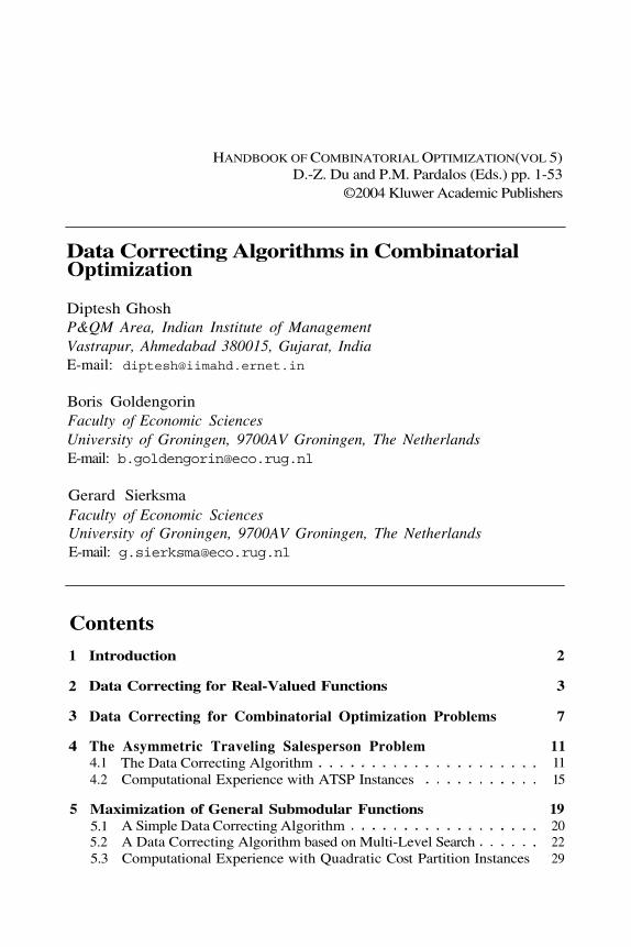
Data Correcting Algorithms in Combinatorial Optimization 1Diptesh Ghosh, Boris Goldengorin, and Gerard Sierksma
The Steiner Ratio of Banach-Minkowski Space - A Survey 55Dietmar Cieslik
Probabilistic Verification and Non-ApproximablityMario Szegedy
83
Steiner Trees in Industry 193Xiuzhen Cheng, Yingshu Li, Ding-Zhu Du, and Hung Q. Ngo
Network-based Model and Algorithms in Data Miningand Knowledge Discovery 217
Vladimir Boginski, Panos M. Pardalos, and Alkis Vazacopoulos
The Generalized Assignment Problem and Extensions 259Dolores Romero Morales and H. Edwin Romeijn
Optimal Rectangular Partitions 313Xiuzhen Cheng, Ding-Zhu Du, Joon-Mo Kim, and Lu Ruan
Connected Dominating Sets in Sensor Networksand MANETs 329
Jeremy Blum, Min Ding, Andrew Thaeler, and Xiuzhen Cheng
Author Index 371
Subject Index 381
HANDBOOK OF COMBINATORIAL OPTIMIZATION(VOL 5)D.-Z. Du and P.M. Pardalos (Eds.) pp. 1-53
©2004 Kluwer Academic Publishers
Data Correcting Algorithms in CombinatorialOptimization
Diptesh GhoshP&QM Area, Indian Institute of ManagementVastrapur, Ahmedabad 380015, Gujarat, IndiaE-mail: [email protected]
Boris GoldengorinFaculty of Economic SciencesUniversity of Groningen, 9700AV Groningen, The NetherlandsE-mail: [email protected]
Gerard SierksmaFaculty of Economic SciencesUniversity of Groningen, 9700AV Groningen, The NetherlandsE-mail: [email protected]
Contents
1
2
3
4
Introduction 2
Data Correcting for Real-Valued Functions 3
7Data Correcting for Combinatorial Optimization Problems
The Asymmetric Traveling Salesperson Problem 111115
19202229
4.14.2
The Data Correcting AlgorithmComputational Experience with ATSP Instances
5 Maximization of General Submodular Functions5.15.25.3
A Simple Data Correcting AlgorithmA Data Correcting Algorithm based on Multi-Level SearchComputational Experience with Quadratic Cost Partition Instances
2 D. Ghosh, B. Goldengorin, and G. Sieksma
6 The Simple Plant Location Problem 3233363941414344454648
6.16.26.36.4
A Pseudo-Boolean Formulation of the SPLPPreprocessing SPLP instancesThe Data Correcting AlgorithmComputational Experience with SPLP Instances6.4.16.4.26.4.36.4.46.4.56.4.6
Testing the Effectiveness of the Reduction Procedure RPBilde and Krarup-type InstancesGalvão and Raggi-type InstancesInstances from the OR-LibraryKörkel-type Instances with 65 SitesKörkel-typeInstances with 100 Sites
References
Introduction1
Polynomially solvable special cases have long been studied in the litera-ture on combinatorial optimization problems (see, for example, Gilmore etal. [19]). Apart from being mathematical curiosities, they often provide im-portant insights for serious problem-solving. In fact, the concluding para-graph of Gilmore et al. [19] states the following, regarding polynomiallysolvable special cases for the traveling salesperson problem.
“ … We believe, however, that in the long run the greatestimportance of these special cases will be for approximation algo-rithms. Much remains to be done in this area.”
This chapter describes a step in the direction of incorporating polynomi-ally solvable special cases into approximation algorithms. We review datacorrecting algorithms — approximation algorithms that make use of poly-nomially solvable special cases to arrive at high-quality solutions. The basicinsight that leads to these algorithms is the fact that it is often easy tocompute a bound on the difference between the costs of optimal solutions totwo instances of a problem, even though it may be hard to compute optimalsolutions for the two instances. These algorithms were first reported in theRussian literature (see Goldengorin [9, 10, 11, 12, 13]).
The approximation in data correcting algorithms is in terms of an ac-curacy parameter, which is an upper bound on the difference between theobjective value of an optimal solution to the instance and that of a solution
Data Correcting Algorithms 3
returned by the data correcting algorithm. Note that this is not expressedas a fraction of the optimal objective value for this instance as in common
algorithms but as actual deviations from the cost of optimal so-lutions.
Although we suggest the use of data correcting algorithms to solve NP-hard combinatorial optimization problems, they form a general problemsolving tool and can be used for functions defined on a continuous domainas well. We will in fact, motivate the algorithm in the next section usinga function defined on a continuous domain, and having a finite range. Wethen show in Section 3, how this approach can be adapted for combinatorialoptimization problems. In the next three sections we describe actual imple-mentation of data correcting algorithms to three problems, the asymmetrictraveling salesperson problem, the maximization of a general submodularfunction, and the simple plant location problem.
2 Data Correcting for Real-Valued Functions
Consider a real-valued function where D is the domain on whichthe function is defined. We assume that is not analytically tractable overD, but is computable in polynomial time for any and concern our-selves with the problem of finding solutions to the function overD, i.e. the problem of finding a member ofwhere and is the pre-defined accuracy parameter.The discussion here is for a minimization problem; the maximization prob-lem can be dealt with in a similar manner.
Let us assume a partition of the domain D. Let us furtherassume that for each of the sub-domains of D, we are ableto find functions which are easy to minimize over and suchthat
We call such easily minimizable functions regular.Theorem 2.1 demonstrates an important relationship between the regular
functions and the original function It states that the function value ofat the best among the minima of all the over their respective domains
is close to the minimum function value of over the domain.
4 D. Ghosh, B. Goldengorin, and G. Sieksma
Theorem 2.1 Let and letThen
Proof: Let Then fori.e. Thus
which proves the result.
Notice that and do not need to be in the same sub-domain of D.Theorem 2.1 forms the basis of the data correcting algorithm to find
an approximate minimum of a function over a certain domain D. Theprocedure consists of three steps: the first in which the domain D of thefunction is partitioned into several sub-domains; the second in which isapproximated in each of the sub-domains by regular functions following thecondition in expression (1) and a minimum point of the regular functionis obtained; and a third step, in which the minimum points computed inthe second step are considered and the best among them is chosen as theoutput. This procedure can be further strengthened by using lower boundsto check if a given sub-domain can possibly lead to a solution better thanany found thus far. The approximation of by regular functions is calleddata correcting, since an easy way of obtaining the regular functions is byaltering the data that describe A pseudocode of the algorithm, which wecall DC-G, is provided below.
Data Correcting Algorithms 5
Lines 5 through 7 in the code carry out the bounding process, and lines8 and 9 implement the process of computing the minima of regular functionsover each sub-domain. These steps are enclosed in a loop, so that at the endof line 10, all the minima of the regular functions are at hand. The code inlines 11 through 16 obtain the best among the minima obtained before. ByTheorem 2.1, the solution chosen by the code in lines 11 through 16 is an
of and therefore, this solution is returned by the algorithmin line 17.
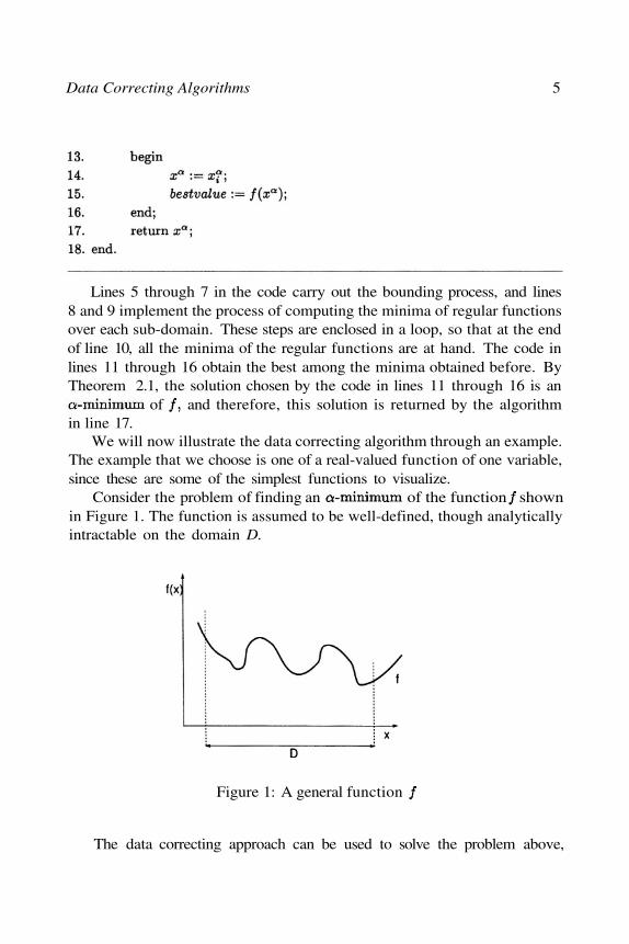
We will now illustrate the data correcting algorithm through an example.The example that we choose is one of a real-valued function of one variable,since these are some of the simplest functions to visualize.
Consider the problem of finding an of the function shownin Figure 1. The function is assumed to be well-defined, though analyticallyintractable on the domain D.
Figure 1: A general function
The data correcting approach can be used to solve the problem above,
6 D. Ghosh, B. Goldengorin, and G. Sieksma
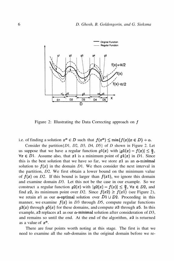
Figure 2: Illustrating the Data Correcting approach on
i.e. of finding a solution such thatConsider the partition{D1, D2, D3, D4, D5} of D shown in Figure 2. Let
us suppose that we have a regular function withAssume also, that is a minimum point of in D1. Since
this is the best solution that we have so far, we store as ansolution to in the domain D1. We then consider the next interval inthe partition, D2. We first obtain a lower bound on the minimum valueof on D2. If this bound is larger than we ignore this domainand examine domain D3. Let this not be the case in our example. So weconstruct a regular function with andfind its minimum point over D2. Since (see Figure 2),we retain as our solution over Proceeding in thismanner, we examine in D3 through D5, compute regular functions
through for these domains, and compute through In thisexample, replaces as our solution after consideration of D3,and remains so until the end. At the end of the algorithm, is returnedas a value of
There are four points worth noting at this stage. The first is that weneed to examine all the sub-domains in the original domain before we re-
Data Correcting Algorithms 7
turn a near-optimal solution using this approach. The reason for this isvery clear. The correctness of the algorithm depends on the result in The-orem 2.1, and this theorem only concerns the best among the minima ofeach of the sub-domains. For instance, in the previous example, if we stopas soon as we obtain the first solution we would be mistaken,since Theorem 2.1 applies to only over The second point isthat there is no guarantee that the near-optimal solution returned by DC-Gwill be in the neighborhood of a true optimal solution. There is in fact,nothing preventing the near-optimal solution existing in a sub-domain dif-ferent from the sub-domain of an optimal solution, as is evident from theprevious example. The true minimum of lies in the domain D5, but DC-Greturns which is in D3. The third point is that the regular functions
approximating do not need to have the same functional form. Forinstance in Example 1, is quadratic, while is linear. Finally, forthe proof of Theorem 2.1, it is sufficient for to be a cover ofD (as opposed to a partition as required in the pseudocode of DC-G).
3 Data Correcting for Combinatorial Optimiza-tion Problems
The data correcting methodology described in the previous section can beincorporated into an implicit enumeration scheme (like branch and bound)and used to obtain near-optimal solutions to NP-hard combinatorial opti-mization problems. In this section we describe how this incorporation isachieved for a general combinatorial optimization problem.
We define a combinatorial optimization problem P as a collection ofinstances I. An instance I consists of a ground set ofelements, a cost vector corresponding to the elementsin G, a set of feasible solutions, and a cost functionThe objective is to obtain a solution, i.e. a member of S that minimizes thecost function. For example, for an asymmetric traveling salesperson problem(ATSP) instance on a digraph G = (V, A), with a distance matrixwe have S is the set of all Hamiltonian cycles in G, and
for eachImplicit enumeration algorithms for combinatorial problems include two
main strategies, namely branching and fathoming. Branching involves parti-tioning the set of feasible solutions S into smaller subsets. This is done underthe assumption that optimizing the cost function over a more restricted so-
8 D. Ghosh, B. Goldengorin, and G. Sieksma
lution space is easier than optimizing it over the whole space. Fathominginvolves one of two processes. First, we could compute lower bounds to thevalue that the cost function can attain over a particular member of the par-tition. If this bound is not better than the best solution found thus far, thecorresponding subset in the partition is ignored in the search for an optimalsolution. The second method of fathoming is by computing the optimumvalue of the cost function over the particular subset of the solution space(if that can be easily computed for the particular subset). We see there-fore that two of the main requirements of the data correcting algorithmpresented in the previous section, i.e. partitioning and bounding, are auto-matically taken care of for combinatorial optimization problems by implicitenumeration. The only other requirement that we need to consider is thatof obtaining regular functions approximating over subsets of the solutionspace.
Notice that the cost function is a function of the cost vector C.So if the values of the entries in C are changed, undergoes a changeas well. Therefore, cost functions corresponding to polynomially solvablespecial cases can be used as “regular functions” for combinatorial optimiza-tion problems. Also note that for the same reason, the accuracy parametercan be compared with a suitably defined distance measure between two costvectors, (or equivalently, two instances). Consider a subproblem in the treeobtained by normal implicit enumeration. The problem instance that isbeing evaluated at that subproblem is a restricted version of the originalproblem instance, i.e., it evaluates the cost function of the original probleminstance for a subset of the original solution space S. If we alter the dataof the problem instance in a way that the altered data corresponds to a poly-nomially solvable special case, while guaranteeing that the cost of an optimalsolution to the altered problem in is not more that an acceptable amounthigher than the cost of an optimal solution to original instance in thenthe altered cost function can be considered to be a regular approximationof the cost function of the original instance in
For combinatorial optimization problems, let us define a proximity mea-sure between two problem instances and as an upper boundfor the difference between and where and are opti-mal solutions to and respectively. The following lemma shows thatthe Hamming distance between the cost vectors of the two instances is aproximity measure when the cost function is of the sum type or the maxtype.
Data Correcting Algorithms 9
Lemma 3.1 If the cost function of an instance I of a combinatorial opti-mization problem is of the sum type, (i.e. or the maxtype, (i.e. then the measure
between two instances and of the problem is an upper bound to thedifference between and where and are optimal solutionsto and respectively.
Proof: We will prove the result for sum type cost functions. The proof formax type cost functions is similar.
For sum type cost functions, it is sufficient to prove the result whenthe cost vectors and differ in only one position. Let for
and Consider any solutionThere are two cases to consider:
In this case,
In this case it is clear that
Therefore, for any solutionwhich automatically implies that as defined in the statement
of Lemma 3.1 is an upper bound for the difference between andwhere and are optimal solutions to and respectively.
At this point, it is important to point out the difference between a fath-oming step and a data correcting step. The bounds used in fathomingsteps consistently overestimate the objective function of optimal solutionsin maximization problems and underestimate it for minimization problems.The amount of over- or underestimation is not bounded. In data correctingsteps however, the “regular function” may overestimate or underestimatethe objective function, regardless of the objective of the problem. However,there is always a bound on the deviation of the “regular function” from theobjective function of the problem.
One way of implementing the data correcting for a NP-hard probleminstance I is the following. We first execute a data correcting step. Weconstruct a polynomially solvable relaxation of the original instance, andobtain an optimal solution to Note that need not be feasible toI. We next construct the best solution to I that we can, starting from
10 D. Ghosh, B. Goldengorin, and G. Sieksma
(If such a solution is not possible, we conclude that the instance doesnot admit a feasible solution.) We also construct an instance of theproblem, which will have as an optimal solution. The proximity measure
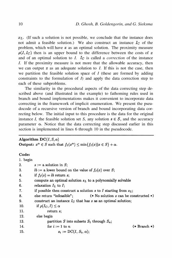
then is an upper bound to the difference between the costs ofand of an optimal solution to I. is called a correction of the instanceI. If the proximity measure is not more that the allowable accuracy, thenwe can output as an adequate solution to I. If this is not the case, thenwe partition the feasible solution space of I (these are formed by addingconstraints to the formulation of I) and apply the data correction step toeach of these subproblems.
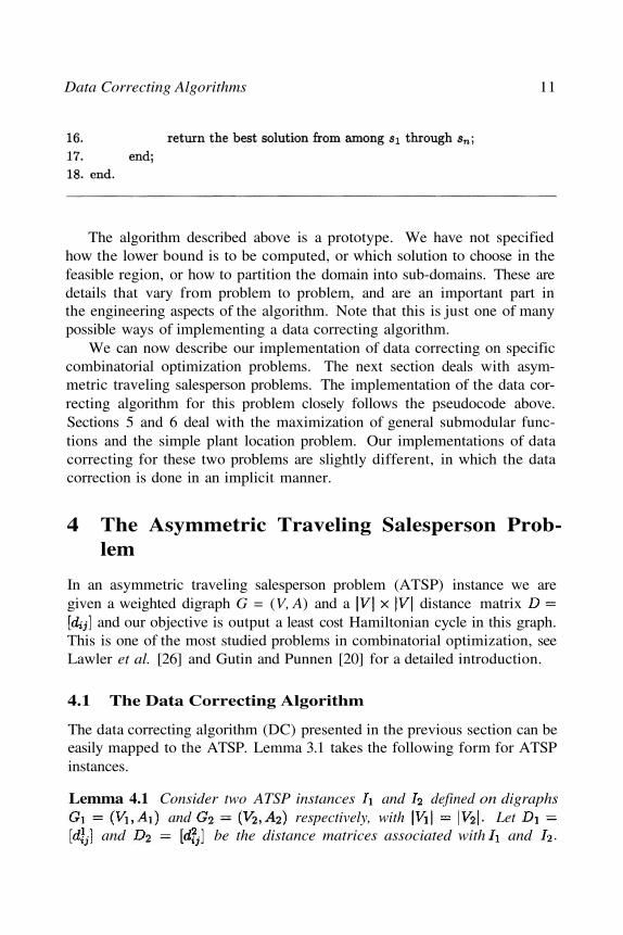
The similarity in the procedural aspects of the data correcting step de-scribed above (and illustrated in the example) to fathoming rules used inbranch and bound implementations makes it convenient to incorporate datacorrecting in the framework of implicit enumeration. We present the pseu-docode of a recursive version of branch and bound incorporating data cor-recting below. The initial input to this procedure is the data for the originalinstance I, the feasible solution set S, any solution and the accuracyparameter Notice that the data correcting step discussed earlier in thissection is implemented in lines 6 through 10 in the pseudocode.
Data Correcting Algorithms 11
The algorithm described above is a prototype. We have not specifiedhow the lower bound is to be computed, or which solution to choose in thefeasible region, or how to partition the domain into sub-domains. These aredetails that vary from problem to problem, and are an important part inthe engineering aspects of the algorithm. Note that this is just one of manypossible ways of implementing a data correcting algorithm.
We can now describe our implementation of data correcting on specificcombinatorial optimization problems. The next section deals with asym-metric traveling salesperson problems. The implementation of the data cor-recting algorithm for this problem closely follows the pseudocode above.Sections 5 and 6 deal with the maximization of general submodular func-tions and the simple plant location problem. Our implementations of datacorrecting for these two problems are slightly different, in which the datacorrection is done in an implicit manner.
4 The Asymmetric Traveling Salesperson Prob-lem
In an asymmetric traveling salesperson problem (ATSP) instance we aregiven a weighted digraph G = (V, A) and a distance matrix
and our objective is output a least cost Hamiltonian cycle in this graph.This is one of the most studied problems in combinatorial optimization, seeLawler et al. [26] and Gutin and Punnen [20] for a detailed introduction.
4.1 The Data Correcting Algorithm
The data correcting algorithm (DC) presented in the previous section can beeasily mapped to the ATSP. Lemma 3.1 takes the following form for ATSPinstances.
Lemma 4.1 Consider two ATSP instances and defined on digraphsand respectively, with Let
and be the distance matrices associated with and
D123456
1-
1910191613
210
-28252222
31610
-131915
4191322
-1313
525131610
-10
62210131911
-
123456
1-90852
20-
18141111
360-284
471
10-00
516470-0
6120380-
12 D. Ghosh, B. Goldengorin, and G. Sieksma
Further let and be optimal solutions to and and let andrespectively represent the lengths of and in instance Then
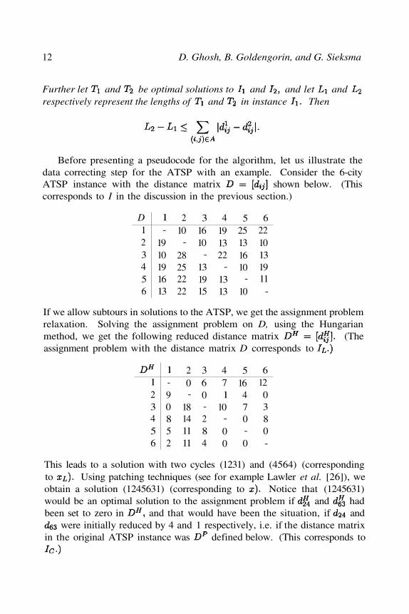
Before presenting a pseudocode for the algorithm, let us illustrate thedata correcting step for the ATSP with an example. Consider the 6-cityATSP instance with the distance matrix shown below. (Thiscorresponds to I in the discussion in the previous section.)
If we allow subtours in solutions to the ATSP, we get the assignment problemrelaxation. Solving the assignment problem on D, using the Hungarianmethod, we get the following reduced distance matrix (Theassignment problem with the distance matrix D corresponds to
This leads to a solution with two cycles (1231) and (4564) (correspondingto Using patching techniques (see for example Lawler et al. [26]), weobtain a solution (1245631) (corresponding to Notice that (1245631)would be an optimal solution to the assignment problem if and hadbeen set to zero in and that would have been the situation, if and
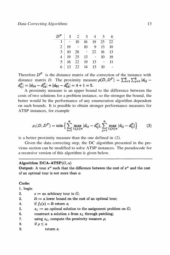
were initially reduced by 4 and 1 respectively, i.e. if the distance matrixin the original ATSP instance was defined below. (This corresponds to
Data Correcting Algorithms 13
123456
1-
1910191613
210
-28252222
31610
-131914
4199
22-
1313
525131610-
10
62210131911
-
Therefore is the distance matrix of the correction of the instance withdistance matrix D. The proximity measure
A proximity measure is an upper bound to the difference between thecosts of two solutions for a problem instance, so the stronger the bound, thebetter would be the performance of any enumeration algorithm dependenton such bounds. It is possible to obtain stronger performance measures forATSP instances, for example
is a better proximity measure than the one defined in (2).Given the data correcting step, the DC algorithm presented in the pre-
vious section can be modified to solve ATSP instances. The pseudocode fora recursive version of this algorithm is given below.
14 D. Ghosh, B. Goldengorin, and G. Sieksma
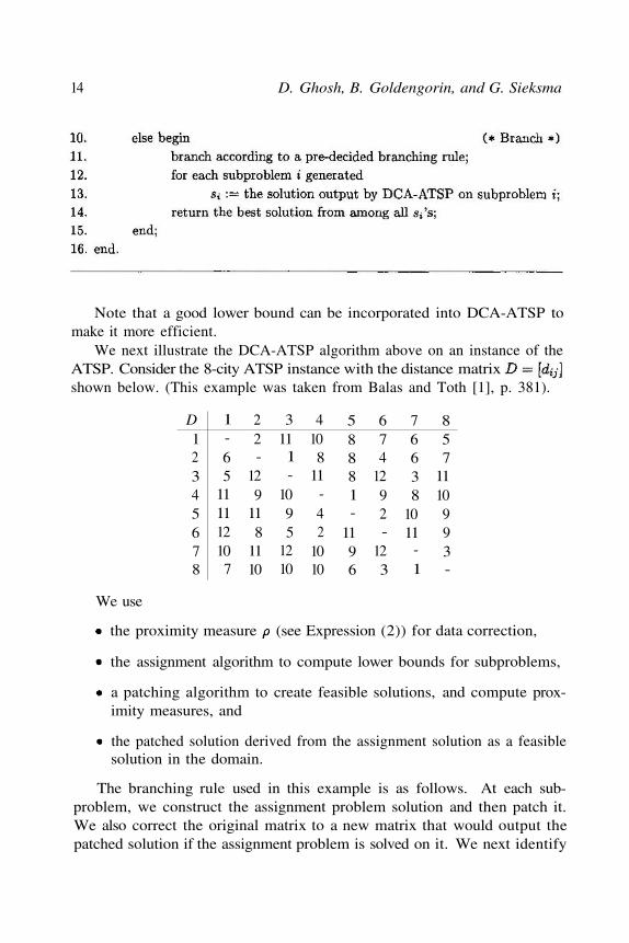
Note that a good lower bound can be incorporated into DCA-ATSP tomake it more efficient.
We next illustrate the DCA-ATSP algorithm above on an instance of theATSP. Consider the 8-city ATSP instance with the distance matrixshown below. (This example was taken from Balas and Toth [1], p. 381).
We use
the proximity measure (see Expression (2)) for data correction,
the assignment algorithm to compute lower bounds for subproblems,
a patching algorithm to create feasible solutions, and compute prox-imity measures, and
the patched solution derived from the assignment solution as a feasiblesolution in the domain.
The branching rule used in this example is as follows. At each sub-problem, we construct the assignment problem solution and then patch it.We also correct the original matrix to a new matrix that would output thepatched solution if the assignment problem is solved on it. We next identify
D12345678
1-65
111112107
22-
129
118
1110
3111-
1095
1210
4108
11-42
1010
58881-
1196
674
1292-
123
76638
1011
-1
857
1110993-
Data Correcting Algorithms 15
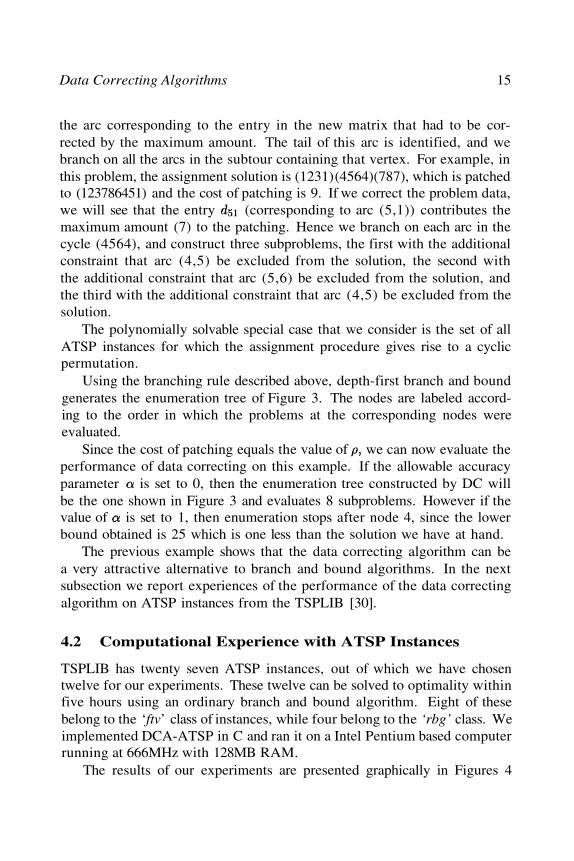
the arc corresponding to the entry in the new matrix that had to be cor-rected by the maximum amount. The tail of this arc is identified, and webranch on all the arcs in the subtour containing that vertex. For example, inthis problem, the assignment solution is (1231)(4564)(787), which is patchedto (123786451) and the cost of patching is 9. If we correct the problem data,we will see that the entry (corresponding to arc (5,1)) contributes themaximum amount (7) to the patching. Hence we branch on each arc in thecycle (4564), and construct three subproblems, the first with the additionalconstraint that arc (4,5) be excluded from the solution, the second withthe additional constraint that arc (5,6) be excluded from the solution, andthe third with the additional constraint that arc (4,5) be excluded from thesolution.
The polynomially solvable special case that we consider is the set of allATSP instances for which the assignment procedure gives rise to a cyclicpermutation.
Using the branching rule described above, depth-first branch and boundgenerates the enumeration tree of Figure 3. The nodes are labeled accord-ing to the order in which the problems at the corresponding nodes wereevaluated.
Since the cost of patching equals the value of we can now evaluate theperformance of data correcting on this example. If the allowable accuracyparameter is set to 0, then the enumeration tree constructed by DC willbe the one shown in Figure 3 and evaluates 8 subproblems. However if thevalue of is set to 1, then enumeration stops after node 4, since the lowerbound obtained is 25 which is one less than the solution we have at hand.
The previous example shows that the data correcting algorithm can bea very attractive alternative to branch and bound algorithms. In the nextsubsection we report experiences of the performance of the data correctingalgorithm on ATSP instances from the TSPLIB [30].
4.2 Computational Experience with ATSP Instances
TSPLIB has twenty seven ATSP instances, out of which we have chosentwelve for our experiments. These twelve can be solved to optimality withinfive hours using an ordinary branch and bound algorithm. Eight of thesebelong to the ‘ftv’ class of instances, while four belong to the ‘rbg’ class. Weimplemented DCA-ATSP in C and ran it on a Intel Pentium based computerrunning at 666MHz with 128MB RAM.
The results of our experiments are presented graphically in Figures 4
16 D. Ghosh, B. Goldengorin, and G. Sieksma
Figure 3: Branch and bound tree for the instance in the example.
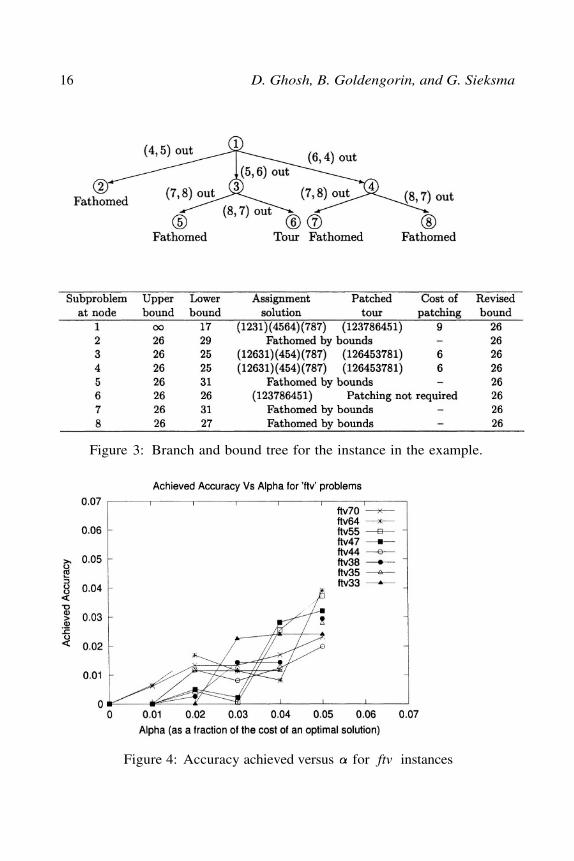
Figure 4: Accuracy achieved versus for ftv instances
Data Correcting Algorithms 17
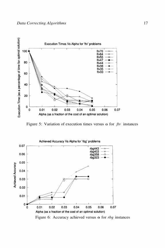
Figure 5: Variation of execution times versus for ftv instances
Figure 6: Accuracy achieved versus for rbg instances
18 D. Ghosh, B. Goldengorin, and G. Sieksma
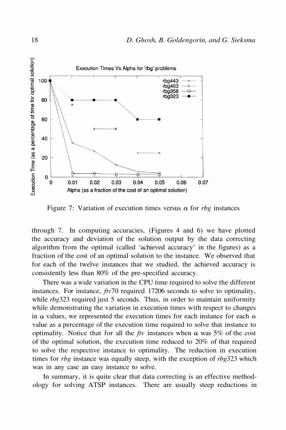
Figure 7: Variation of execution times versus for rbg instances
through 7. In computing accuracies, (Figures 4 and 6) we have plottedthe accuracy and deviation of the solution output by the data correctingalgorithm from the optimal (called ‘achieved accuracy’ in the figures) as afraction of the cost of an optimal solution to the instance. We observed thatfor each of the twelve instances that we studied, the achieved accuracy isconsistently less than 80% of the pre-specified accuracy.
There was a wide variation in the CPU time required to solve the differentinstances. For instance, ftv70 required 17206 seconds to solve to optimality,while rbg323 required just 5 seconds. Thus, in order to maintain uniformitywhile demonstrating the variation in execution times with respect to changesin values, we represented the execution times for each instance for eachvalue as a percentage of the execution time required to solve that instance tooptimality. Notice that for all the ftv instances when was 5% of the costof the optimal solution, the execution time reduced to 20% of that requiredto solve the respective instance to optimality. The reduction in executiontimes for rbg instance was equally steep, with the exception of rbg323 whichwas in any case an easy instance to solve.
In summary, it is quite clear that data correcting is an effective method-ology for solving ATSP instances. There are usually steep reductions in
Data Correcting Algorithms 19
execution times even when the allowed accuracy is very small. This makesthe method very useful for solving real world problems where a near-optimalsolution is often acceptable provided the execution times are not too long.
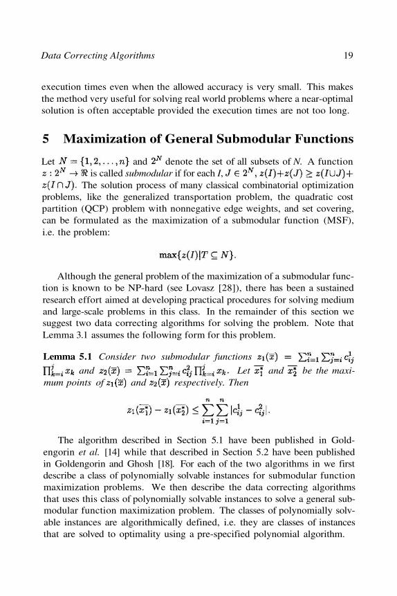
5 Maximization of General Submodular Functions
Let and denote the set of all subsets of N. A functionis called submodular if for each I,
The solution process of many classical combinatorial optimizationproblems, like the generalized transportation problem, the quadratic costpartition (QCP) problem with nonnegative edge weights, and set covering,can be formulated as the maximization of a submodular function (MSF),i.e. the problem:
Although the general problem of the maximization of a submodular func-tion is known to be NP-hard (see Lovasz [28]), there has been a sustainedresearch effort aimed at developing practical procedures for solving mediumand large-scale problems in this class. In the remainder of this section wesuggest two data correcting algorithms for solving the problem. Note thatLemma 3.1 assumes the following form for this problem.
Lemma 5.1 Consider two submodular functions
and Let and be the maxi-mum points of and respectively. Then
The algorithm described in Section 5.1 have been published in Gold-engorin et al. [14] while that described in Section 5.2 have been publishedin Goldengorin and Ghosh [18]. For each of the two algorithms in we firstdescribe a class of polynomially solvable instances for submodular functionmaximization problems. We then describe the data correcting algorithmsthat uses this class of polynomially solvable instances to solve a general sub-modular function maximization problem. The classes of polynomially solv-able instances are algorithmically defined, i.e. they are classes of instancesthat are solved to optimality using a pre-specified polynomial algorithm.
20 D. Ghosh, B. Goldengorin, and G. Sieksma
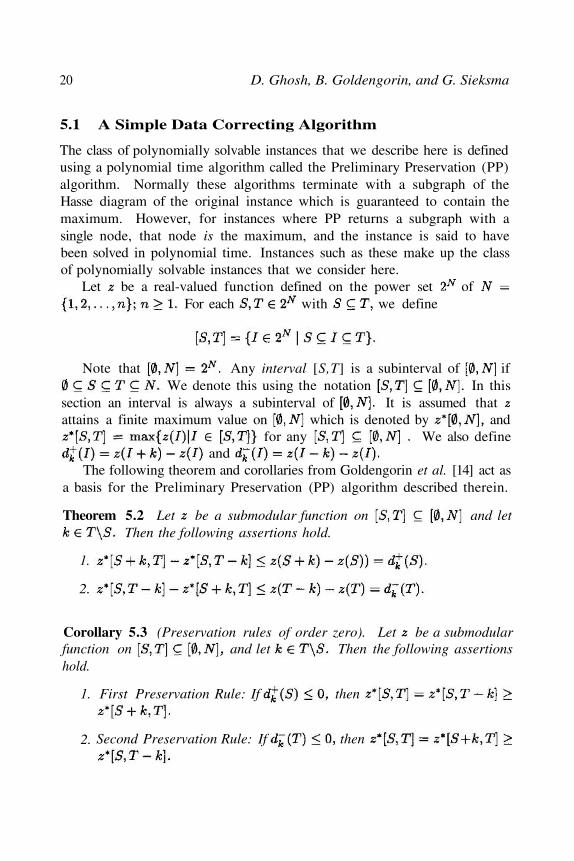
5.1 A Simple Data Correcting Algorithm
The class of polynomially solvable instances that we describe here is definedusing a polynomial time algorithm called the Preliminary Preservation (PP)algorithm. Normally these algorithms terminate with a subgraph of theHasse diagram of the original instance which is guaranteed to contain themaximum. However, for instances where PP returns a subgraph with asingle node, that node is the maximum, and the instance is said to havebeen solved in polynomial time. Instances such as these make up the classof polynomially solvable instances that we consider here.
Let be a real-valued function defined on the power set ofFor each with we define
Note that Any interval [S,T] is a subinterval of ifWe denote this using the notation In this
section an interval is always a subinterval of It is assumed thatattains a finite maximum value on which is denoted by and
for any We also defineand
The following theorem and corollaries from Goldengorin et al. [14] act asa basis for the Preliminary Preservation (PP) algorithm described therein.
Corollary 5.3 (Preservation rules of order zero). Let be a submodularfunction on and let Then the following assertionshold.
Theorem 5.2 Let be a submodular function on and letThen the following assertions hold.
1.
2.
1.
2.
First Preservation Rule: If then
Second Preservation Rule: If then
Data Correcting Algorithms 21
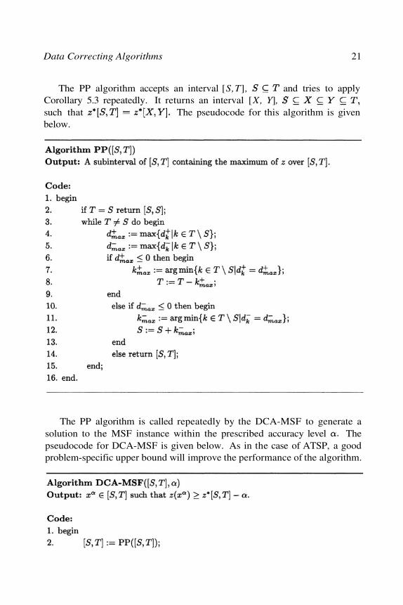
The PP algorithm accepts an interval [S,T], and tries to applyCorollary 5.3 repeatedly. It returns an interval [X, Y],such that The pseudocode for this algorithm is givenbelow.
The PP algorithm is called repeatedly by the DCA-MSF to generate asolution to the MSF instance within the prescribed accuracy level Thepseudocode for DCA-MSF is given below. As in the case of ATSP, a goodproblem-specific upper bound will improve the performance of the algorithm.
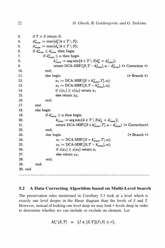
22 D. Ghosh, B. Goldengorin, and G. Sieksma
5.2 A Data Correcting Algorithm based on Multi-Level Search
The preservation rules mentioned in Corollary 5.3 look at a level which isexactly one level deeper in the Hasse diagram than the levels of S and T.However, instead of looking one level deep we may look levels deep in orderto determine whether we can include or exclude an element. Let
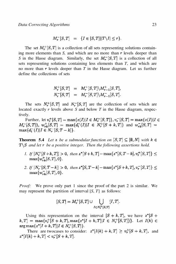
Data Correcting Algorithms 23
The set is a collection of all sets representing solutions contain-ing more elements than S, and which are no more than levels deeper thanS in the Hasse diagram. Similarly, the set is a collection of allsets representing solutions containing less elements than T, and which areno more than levels deeper than T in the Hasse diagram. Let us furtherdefine the collections of sets
The sets and are the collection of sets which arelocated exactly levels above S and below T in the Hasse diagram, respec-tively.
Further, letand
Theorem 5.4 Let be a submodular function on withand let be a positive integer. Then the following assertions hold.
1.
2.
If then
If then
Proof: We prove only part 1 since the proof of the part 2 is similar. Wemay represent the partition of interval [S, T] as follows:
Using this representation on the interval we haveLet
There are twocases to consider: and
24 D. Ghosh, B. Goldengorin, and G. Sieksma
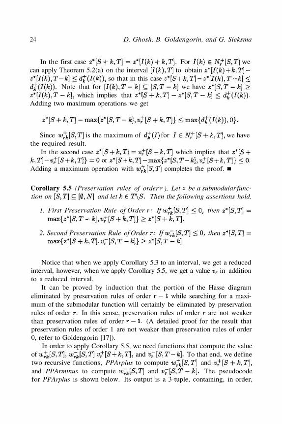
In the first case For wecan apply Theorem 5.2(a) on the interval to obtain
so that in this caseNote that for we have
which implies thatAdding two maximum operations we get
Since is the maximum of for we havethe required result.
In the second case which implies thator
Adding a maximum operation with completes the proof.
Corollary 5.5 (Preservation rules of order Let be a submodular func-tion on and let Then the following assertions hold.
1.
2.
First Preservation Rule of Order If then
Second Preservation Rule of Order If then
Notice that when we apply Corollary 5.3 to an interval, we get a reducedinterval, however, when we apply Corollary 5.5, we get a value in additionto a reduced interval.
It can be proved by induction that the portion of the Hasse diagrameliminated by preservation rules of order while searching for a maxi-mum of the submodular function will certainly be eliminated by preservationrules of order In this sense, preservation rules of order are not weakerthan preservation rules of order (A detailed proof for the result thatpreservation rules of order 1 are not weaker than preservation rules of order0, refer to Goldengorin [17]).
In order to apply Corollary 5.5, we need functions that compute the valueof and To that end, we definetwo recursive functions, PPArplus to compute andand PPArminus to compute and The pseudocodefor PPArplus is shown below. Its output is a 3-tuple, containing, in order,
).