handbook for collecting vegetation plot data in...

handbook for collectingVegetation Plot Data in Minnesota:

Relevé Method

2nd Edition

the

handbook for collectingVegetation Plot Data in Minnesota:

Relevé Methodthe

2nd Edition

Minnesota Biological SurveyMinnesota Natural Heritage and Nongame Research ProgramEcological Land Classification ProgramMinnesota Department of Natural Resources

Minnesota Department of Natural Resources. 2013. A handbook for collecting vegetation plot data in Minnesota: The relevé method. 2nd ed. Minnesota Bio-logical Survey, Minnesota Natural Heritage and Nongame Research Program, and Ecological Land Classification Program. Biological Report 92. St. Paul: Minnesota Department of Natural Resources.

©2013. State of Minnesota, Department of Natural Resources

For More Information Contact:DNR Information Center500 Lafayette RoadSt. Paul, MN 55155 - 4040(651) 296-6157 (Metro Area)1-888-MINNDNR (1-888-646-6367)

TTY(651) 296-5484 (Metro Area)1-800-657-3929www.mndnr.gov

Equal opportunity to participate in and benefit from programs of the Minnesota Department of Natural Resources is available to all individuals regardless of race, color, creed, religion, national origin, sex, marital status, status with regard to public assistance, age, sexual orientation, membership or activity in a local commission, or disability. Discrimination inquiries should be sent to MN DNR, 500 Lafayette Road, St. Paul, MN 55155-4031; or the Equal Opportunity Office, Department of the Interior, Washington, DC 20240.

Funding provided by the Minnesota Legislature, with partial funding provided by the Minnesota Environment and Natural Resources Trust Fund as recom-mended by the Legislative-Citizen Commission on Minnesota Resources.

Preface

The first edition of this handbook was published in 2007 by the Minnesota Biological Survey, the Minnesota Natural Heritage and Nongame Research Program, and the Ecological Land Classification Program of the Minnesota Department of Natural Resources (DNR) to aid in collection and use of relevés in Minnesota. The first edition updated the DNR’s original handbook for collect-ing relevés, compiled by John Almendinger in 1987 (DNR 1987). The current (second) edition of this handbook differs from the first mostly in minor changes to make its organization consistent with a recent redesign of the DNR’s Relevé Database and with several modifications to the DNR’s relevé field form sug-gested by ecologists.

Relevé sampling is a flexible and powerful tool for collecting information on and detecting patterns in vegetation. Relevé sampling has been used extensively by vegetation scientists in the DNR for more than two decades, primarily for describing and classifying native plant communities. To facilitate widespread vegetation study in Minnesota using relevés, the DNR has developed a da-tabase that currently contains electronic versions of more than 9,000 relevés and other very similar kinds of vegetation plot data from across Minnesota, as well as 670 vegetation plots from adjacent parts of Ontario. The largest percentage of the relevés in the database were collected by plant ecologists and botanists working for the DNR, but the relevé database also contains many relevés collected by researchers at universities, private organizations, and other government agencies. Approximately 980 of the plots in the DNR’s relevé database have been contributed to the Ecological Society of America’s national vegetation plot database (VegBank). It is hoped that more, if not all, of Minnesota’s relevés will be supplied to the national database in the future, should resources for data transfer become available.

This handbook provides standards for collection in Minnesota of relevés that are used for description and classification of native plant communities. Much of the information, however, applies to relevé collection in general and should be useful to researchers working on other kinds of vegetation studies that require plot-based sampling. Researchers using methodology comparable to that of the DNR would be in position to enhance their datasets with samples from the DNR’s relevé database. In turn, the relevés they contribute to the DNR’s database may help improve description, classification, and understand-ing of Minnesota’s native vegetation. Appendices A and B of this handbook provide information on contributing samples to and obtaining data from the DNR’s relevé database.

i

Contents

Preface .................................................................................................... i

1. Introduction ........................................................................................1 Definition ..............................................................................................1 History .................................................................................................1 Use of Relevés ....................................................................................2

2. Methods ..............................................................................................5 Relevé Plot Location ............................................................................5 Relevé Plot Size and Shape ................................................................6 Recording the Relevé Location ............................................................8 Delineating the Relevé Plot .................................................................8 Recording Data ....................................................................................8 Site Data Fields .................................................................................10 Vegetation Data .................................................................................25 General Overview ..........................................................................25 Physiognomic Group Variables ......................................................30 Species Occurrence Data Variables ..............................................33

Appendices ..........................................................................................39 A. Contributing Samples to the DNR Relevé Database ...................39 B. Obtaining Data from the DNR Relevé Database .........................39 C. Obtaining a Copy of the DNR Relevé Field Form ........................39 D. Delineating a Square Relevé Plot ................................................40 E. List of Institutions .........................................................................41 F. List of Ownerships .......................................................................41 G. Invasive Earthworm Rapid Assessment ......................................42 H Key to Soil Drainage Classes ......................................................45 I. Key to Mineral Soil Texture ..........................................................46 J. Characteristics of Wetland Organic Soils ....................................47 K. Plant Species Commonly Assigned Incorrect Life-Form Codes ..48 References ...........................................................................................49

ii

1. Introduction

DefinitionThe word relevé (rel-ә-vā), of French origin, translates into “list,” “statement,” or “summary,” among the English meanings most relevant to its use in vegetation study. In this manual, a relevé is defined as a list of the plants in a delimited plot of vegetation, with information on species cover and on substrate and other abiotic features in the plot. Typically the vegetation is stratified into height layers by life forms (such as deciduous woody plants, forbs, graminoids, etc.) to describe the apparent vertical structure of the vegetation. In each layer each species is assigned a cover or abundance value based on its representation in that layer. Note that in this definition it is not specified how the placement of the plot in the vegetation is to be determined nor how the plot samples, or is related to, the surrounding vegetation. The relevé is simply any kind of plot with a list of the species in the plot, their cover or abundance, and some indication of the structure of the vegetation according to height classes and life forms.1

HistoryRelevés are closely associated with a procedure for describing and classifying vegetation that has a long history of development and use among European plant ecologists engaged in phytosociological studies.2 This procedure, docu-mented in what is essentially its current form in the early 1900s by the Swiss biologist J. Braun-Blanquet (Poore 1955a), involves describing or character-izing recognizable units in the vegetation of a region by the description or characterization of the vegetation in a single representative standard plot—a relevé—within each unit. The relevés from many units are then analyzed to develop descriptions and classifications of the vegetation in the study region.

Although developed for use in conjunction with the above-described method of vegetation characterization, relevés have been increasingly used in other kinds of vegetation studies as a practical, relatively fast means of collecting information on vegetation. Relevés have been most widely used in Europe, particularly in studies involving vegetation classification, and the technique has also been employed in regions of Asia, Africa, South America, and, in-creasingly, North America (Benninghoff 1966, Westhoff and van der Maarel 1978, Mucina et al. 1993, Rodwell et al. 1995, Barbour et al. 1999, Box 1999, Jennings et al. 2004). The list of references at the end of this handbook in-cludes examples of vegetation studies in North America that have used relevé data (see, for example, Klinka et al. 1996, Peinado et al. 1998, Emrick and Hill 1999, Rivas-Martinez et al. 1999, Mack et al. 2000, Stachurska-Swakon and Spribille 2002, Tomback et al. 2005).1There appears to be variation among plant ecologists in application of the term relevé. For some, relevé is applied to any kind of plot-based vegetation sample that incorporates information on species presence and cover (see, for example, Knapp 1984c). For many if not most, however, relevé is applied to a vegetation plot linked to a specific approach to describing plant communities that involves 1) determination of the minimal plot area needed to capture most species in the community (see page 6) and 2) subjectively placing plots in sample plant community stands to most efficiently characterize the vegetation in a study area (see page 2).2The field of phytosociology was first defined in the late 1800s as the study of the sociological relationships of plants (Barbour et al. 1999), and has more recently been defined as the study of vegetation, including floristic composition, structure, development, and distribution (see, for example, Poore 1955a, Becking 1957, or Mueller-Dombois and Ellenberg 1974).

1

Relevés were first used in vegetation study in Minnesota by researchers at the University of Minnesota in the early 1960s (Janssen 1967). Since then, numer-ous studies in Minnesota have used relevé sampling or very similar sampling methods, with E. Cushing of the University of Minnesota especially influential in the adoption of the technique in the state. Most of the studies in Minnesota have been done to characterize, classify, or describe the range of variation in vegetation in study project areas (see, for example, Janssen 1967, Glaser et al. 1981, Almendinger 1985, Mason 1994, Stai 1997, U.S. Geological Survey 2001). Other studies have been done to establish baseline data on vegetation in the vicinity of proposed industrial developments or mining projects (Glaser and Wheeler 1977, Sather 1980), for characterization of rare plant or rare ani-mal species habitat (Johnson-Groh 1997, Lane 1999), and to develop indices of biotic integrity for selected vegetation types or habitats (Galatowitsch et al., Galatowitsch et al. 2000, Gernes and Helgen 2002). Relevé plots have also been established in Minnesota for use in plant or vegetation monitoring, and the data from accumulated relevé plots have been used to develop species lists for restoration of native plant communities (Lane and Texler 2009).

The Minnesota Biological Survey (MBS), Natural Heritage and Nongame Research Program (NHNRP), and Ecological Land Classification Program (ELCP) of the Minnesota Department of Natural Resources (DNR) have col-lected relevés mainly for development and refinement of a native plant commu-nity classification used in guiding native vegetation survey work and research (DNR 1993, 2003, 2005a, 2005b). In 1987, the NHNRP and MBS established a database for relevés collected in Minnesota and have since assembled more than 9,000 relevés from many sources, going back to the first relevés done in Minnesota in the 1960s. Most of the relevés in the database have been done by surveyors with the MBS, NHNRP, and ELCP in accordance with the meth-odology described in Chapter 2 of this handbook. This methodology follows that of Braun-Blanquet, with some modifications instituted by researchers at the University of Minnesota (especially E. Cushing) and at the DNR.

Use of RelevésUsing relevés for vegetation study involves two broad considerations. One is the method by which relevé plots are placed in the study area. The second is how the data on plant species cover are collected in the plot. Both of these considerations are influenced by the objectives and requirements of the study.

Methods of plot placement in relevé studies can be separated into two gen-eral categories, subjective and objective. In a typical relevé study involving subjective plot placement, the surveyor divides the study area into sample stands based on plant community units identified during fairly intensive re-connaissance done prior to sampling with relevé plots. A single relevé plot is then placed at a carefully chosen site within each sample stand so that the data from the plot represent the attributes of the stand as a whole. Subjective plot placement is used most commonly in studies whose goal is to describe or characterize vegetation—for example, in developing plant community clas-sifications. In the hands of a field researcher familiar with the vegetation in a study area, subjective plot placement is argued to yield suitable classifications in less time and using fewer plots than studies using objective plot placement and therefore is presented as a more efficient alternative (see, for example,

2

Moore et al. 1970 or Becking 1957). The data collected using subjective plot placement are not suitable for analysis using probability statistics, although they can be summarized or described using numerical techniques such as ordination and classification.

The utility of subjective plot placement is made evident by considering proj-ects whose aim is to describe or classify native vegetation in fragmented landscapes; this has been a significant application of the technique in the DNR. In such studies, the purpose is to characterize as faithfully as possible undisturbed examples of the vegetation, which requires deliberately placing plots away from field edges, clearcuts, roadsides, and other anthropogenically disturbed areas that may influence species composition in nearby parts of the stand and cloud the results of analyses. Subjective plot placement also allows for adequate characterization of rare or minor plant community types in a study area, which tend to be undersampled in vegetation studies using ob-jective plot placement (Barbour et al. 1999, Smartt 1978). In general, in relevé studies that utilize subjective plot placement, the quality and usefulness of the resulting descriptions or classifications of vegetation depend greatly on the surveyor’s field skills and on identifying stands and placing samples so that they evenly capture the full range of variation in vegetation in a study area. The surveyor must remain open-minded about the initial division of the study area into sample stands and be prepared to adjust the initial sampling criteria and units if it becomes evident that certain recurring community types were not recognized during preliminary reconnaissance (Mueller-Dombois and El-lenberg 1974).

In studies using objective plot placement, sample plots are placed either randomly or at regular intervals (i.e., systematically) across the entire study area, or alternatively the study area is divided into general units according to broad vegetation types, groupings of dominant species, substrate types, management units, or other general criteria and plots are placed randomly or systematically within these units; the latter are examples of stratified random or stratified systematic sampling. In general, objective placement of plots is used in experimental (rather than descriptive) studies, where the goals of the study require that the data collected be treatable with probability statistics. Ex-amples might include a vegetation monitoring study in which one is concerned with detecting statistically significant change over time within stands, a study in which one is looking for statistically significant differences across sample stands in a landscape, or a study using correlation or regression techniques to test the relationship of plant communities and environmental factors. A dis-cussion of study design using objective plot placement is beyond the scope of this manual, but a starting point for general information might include Mueller-Dombois and Ellenberg (1974), Greig-Smith (1983), or Bonham (1989).

The second broad consideration in use of relevés concerns the determination of cover of plant species within a relevé plot: whether it is estimated by eye or by mechanical means. Choosing between ocular and mechanical estima-tion of cover is influenced by the requirements of a study, weighing the time and resources available to collect data versus issues such as repeatability of observation and resolution of the data collected. Estimates of cover by eye are typically done when time and resources for collection of data are limited

3

(relative to the size of the study area and the range of vegetation to be sam-pled) and the data are to be used for descriptive purposes such as vegetation classification. Ocular estimates of cover are usually made using a scale with fairly broad cover classes such as the Braun-Blanquet scale, which has seven categories for estimating species abundance and cover. The relatively broad categories in the scale help to promote agreement among different observers when estimating cover. Broad, rather than narrow, categories may also be more appropriate for describing species that vary greatly in cover over the course of a growing season or from season to season; in this way one does not give a false sense of exactness to an ephemeral variable (Barbour et al. 1999, McCune and Grace 2002). Cover data collected by visual estimation using the Braun-Blanquet or similar scales can be analyzed mathematically and are considered semi-quantitative. The use of broad categories, however, can make the data collected unsuitable for statistical analyses if certain as-sumptions are not met (Bonham 1989). The data may also lack the resolution necessary to detect fine-scale variation in species cover over time (such as in monitoring studies) or along an environmental gradient (Pakarinen 1984).

In studies requiring collection of statistically rigorous data, species cover can be estimated in the plot using methods that incorporate mechanical measure-ments, such as point, line-intercept, or photographic methods. When data are estimated by mechanical means rather than strictly by eye, the surveyor also may reliably record percent cover along a finely divided scale (for example, in 1% increments of cover) and need not rely on the broad classes used when estimating cover by eye. Cover data collected using mechanical measure-ments are considered quantitative, as the measurements minimize subjective judgments made by the observer (Bonham 1989). In comparison with ocular estimation, mechanical estimation of species cover generally increases the time required to complete collection of data within an individual plot. For more information on collecting species cover data, see Kershaw (1973), Mueller-Dombois and Ellenberg (1974), or Bonham (1989).

For those interested in more context on use of relevés, as a starting point Ben-ninghoff (1966) has a short summary of the basic method from a North Ameri-can perspective; Poore (1955a, 1955b, 1955c, 1956) has a longer description and philosophical analysis of the relevé method; and Westhoff and van der Maarel (1978) and Becking (1957) provide an overview of the history and gen-eral concepts of the Braun-Blanquet approach to vegetation description and classification using relevés, with Becking’s discussion prompted by an inter-est in comparing the approach of European phytosociologists to vegetation study with that of American ecologists. Detailed discussions of relevé meth-ods and use of relevés in specific kinds of vegetation sampling are presented by various authors in Knapp (1984). The discussion in Tomback et al. (2005) provides examples of the considerations weighed in determining whether and how to use relevés in a particular study. Jennings et al. (2004) place the Braun-Blanquet approach in context with other vegetation sampling and classifica-tion approaches used in North America and also have an overview of issues concerning sampling design, plot placement, and estimation of cover, among other aspects of sampling. Useful descriptions and discussions of vegetation sampling methods in general are available in Mueller-Dombois and Ellenberg (1974), Greig-Smith (1983), Bonham (1989), Kent and Coker (1992), and Bar-bour et al. (1999).

4

2. Methods

Relevé Plot LocationSurveyors with the Natural Heritage and Nongame Research Program, Min-nesota Biological Survey, and Ecological Land Classification Program of the DNR do relevés primarily for use in characterizing or classifying native veg-etation and follow the basic methods developed by Braun-Blanquet. Survey-ors first divide the landscape into units, most often according to native plant communities.1 These units are identified using aerial photo interpretation, field experience in the study area, and other information (such as soils or surficial geology maps), and are transcribed onto topographic maps. Surveyors then begin field assessment of the plant community units, using the information transcribed onto the maps as a guide. The suitability of any plant community occurrence (or sample stand) for siting a relevé plot is determined by the qual-ity of the vegetation and the absence of signs of human-related disturbance. An attempt is also made to select community occurrences or sample stands such that one captures all of the possible variability of the plant community within a given landscape or geographic region. This is done by distributing relevés among occurrences of the community that vary in habitat characteris-tics such as substrate, slope position, soils, and so on. In some landscapes, some community types may have few high-quality occurrences and it may not be possible for the surveyor to find enough sample stands to capture the full range of natural variation of the community. For example, good-quality remnants of deciduous forest in the agricultural regions of Minnesota are often limited to steep, untillable slopes, while forests on level sites, which may have differed in plant species composition from those on slopes, may be absent or too disturbed to sample as native plant communities.

When a surveyor decides to do a relevé within a given stand, the criteria used in siting the plot are: 1) the site is representative of the stand as a whole; 2) the site is uniform in vegetation composition and structure as well as in habitat type (considering soil moisture, substrate, aspect, hydrology, and so on); 3) the vegetation in the plot area is ecologically intact and has not been visibly disturbed by human-related activity such as recent logging, heavy grazing, or invasion by non-native species; and 4) the plot is not close to any noticeable ecotone or boundary between different types of vegetation. If there is variation in the vegetation in the vicinity of the plot, the surveyor records some impres-sions on the relevé field form about the different vegetation types present and the nature of the boundaries between them (diffuse, sharp, etc.; see Figure 2 on page 9 for a sample copy of the DNR’s relevé field form). The surveyor also commonly notes which environmental factors may be causing the apparent vegetation pattern. The importance in classification studies of placing relevé plots in areas uniform in vegetation and habitat cannot be overly emphasized. If a relevé plot does contain a small area that clearly differs from the vegetation

1The initial classifications of native plant communities used by the DNR in vegetation studies were based on review of available literature in Minnesota and adjacent regions and on field observations made by NHNRP and MBS plant ecologists (Wendt 1984, DNR 1993). These classifications have since been supplanted by a classification based in large part on analysis of relevé data collected in plant communities across Minnesota (see DNR 2003, 2005a, or 2005b). For a general discussion of the process of dividing a landscape or study area into units to be sampled, see Mueller-Dombois and Ellenberg (1974). (Note: it is not necessary to know the type of native plant community for the relevé to be suitable for classification, only that the community represents an association of native plants that repeats on the landscape and does not appear to be an artifact of human activity or some other unique or ephemeral event or set of events.)

5

of the rest of the plot—such as a small wet depression in an upland forest—the presence of the atypical area is noted on the field form.

On occasion, relevé plots are placed deliberately to include different vegeta-tion types as, for example, when two distinct vegetation types are strongly as-sociated with one-another and are repeated on the landscape in a predictable pattern. In these cases, it is usually indicated on the field form that the purpose of the relevé is to characterize this association of vegetation types. DNR sur-veyors also do relevés for purposes other than classification of native vegeta-tion, such as characterizing the habitats of rare plants or describing ecotonal areas. In these cases, the sample stands or the plot sites may be determined by criteria different from those used for classification purposes—this is usually indicated by the surveyor on the relevé data sheet.

Relevé Plot Size and ShapeEach relevé plot should be large enough to include most species regularly distributed through the sample stand. The appropriate relevé plot size for a particular type of vegetation in theory can be determined by constructing a species-area curve. This is often done by sampling nested plots in a homoge-neous area in a representative stand of the vegetation type and then graphing the number of species recorded against plot size (Fig. 1). For vegetation in temperate regions, the species-area curve tends to be steep initially and then levels in number of species as the plot size increases. The intersection of plot size with the point at which the curve appears to level yields the minimal sample area. Ideally, this process is repeated in several representative stands of the vegetation type, with the largest resulting minimal area then used as a guide for relevé plot size (Mueller-Dombois and Ellenberg 1974; see also Kershaw [1973] for a discussion of the subjectivity associated with assessing homogeneity of vegetation and establishing minimal sample area; and Greig-Smith [1983] for a critique of using nested rather than randomly placed plots for developing the species-area curve, as well as a critique of the minimal area concept itself).

In practice, the minimal sample area is generally correlated with the life-forms of plants and the structure of the vegetation, so it is not necessary to deter-mine minimal relevé sizes for each new study. Guidelines for relevé size based on species-area curve investigations for different types of vegetation are giv-en in Mueller-Dombois and Ellenberg (1974), Westhoff and van der Maarel (1978), and Knapp (1984c) (see Table 1). Chytry and Otypkova (2003) have a review and discussion of plot sizes historically used in Europe. For Minnesota, a 400 square-meter plot in wooded vegetation and a 100 square-meter plot in treeless vegetation generally exceed the minimal sample area. Peet et al. (1998) present an approach to plot layout that incorporates an array of 10-me-ter by 10-meter modules and allows for flexibility in size and intensity of area sampled, depending on the requirements of the study.

DNR surveyors typically use square relevé plots—20 x 20 meters in upland forests, woodlands, savannas, and forested wetlands, and 10 x 10 meters in prairies, shrub swamps, and open wetlands. The shape of the plot and its orientation (if irregularly shaped) are important mainly in vegetation with regu-lar or periodic patterns at scales finer than the plot size. For example, in the

6

Figure 1. System of nested plots for determining minimal relevé area and hypothetical species-area curve derived from a survey of nested plots. In general, a relevé plot is considered sufficiently large when doubling the sample area results in an increase of less than 10% in number of species (after Mueller-Dombois and Ellenberg 1974).

string bogs of Minnesota, which consist of alternating peat ridges and flooded troughs, the ridges and troughs may be sufficiently narrow that a 10 x 10 meter relevé plot would always contain a portion of both a trough and a ridge. If the surveyor wanted to contrast the vegetation of these two features, it would be appropriate to use rectangular relevé plots, laying out each plot entirely on ei-ther a ridge or in a trough. Alternatively, if the vegetation of the area as a whole was to be compared with some other type of bog vegetation, placing rectan-gular plots transversely across the ridges and troughs would be appropriate.

7

1 meter

1 2

34

5

6

7

8

9

# of

spe

cies

2 4 8 16 32 64 area (m2)

4 5 6 7 8 9 # of plots

8

vegetation type example in Minnesota area (sq. meters)

temperate deciduous forestsouthern mesic maple-basswood forest

100 - 500central dry-mesic oak-aspen forest

boreal coniferous forestnorthern poor conifer swamp

100 - 500northern dry-sand pine woodland

shrub communitynorthern bedrock shrubland

10 - 250mesic brush-prairie

grassland southern dry prairie 25 - 100

Relevé shape might also be altered when sampling vegetation that varies in relation to slope or aspect. In general, the shape of the plot is dictated by the specific purpose of the vegetation study, although where feasible square plots are preferable to oblong or irregularly shaped plots because square plots have lower ratios of edge-to-plot area.

Recording the Relevé LocationAfter deciding on the location, size, and shape of the relevé plot, the plot loca-tion is determined using a GPS unit or, if the surveyor does not have a GPS unit, the location is recorded on the surveyor’s field map (usually a 7.5 minute United States Geological Survey [USGS] topographic map). The location can also be recorded on an aerial photograph if aerial photos are being used for orientation in the field. Later, the GPS coordinates can be used to create a map showing the location of the plot, or photocopies of the surveyor’s field map or aerial photograph can be attached to the field form, expediting entry of location information into the DNR’s Natural Heritage Information System elec-tronic relevé database and providing a clear record of the plot location. Often, it is helpful to provide a sketch showing the relation of the plot to unmapped features (such as trails, fencelines, buildings, clearcuts, or ponds) that might aid in relocating the plot. This sketch is usually attached to the original field form and archived in the DNR’s manual relevé file.

Delineating the Relevé PlotThe final step before recording field data is delineating the relevé plot. For most work, the plot boundaries and corners can be established by measur-ing with a tape along the perimeter of the plot and turning 90o at each corner with the aid of a field compass. A 10 x 10 meter plot laid out in this way is generally within 3 square meters of 100 square meters in size. (More accurate techniques for delineating plots are described in Appendix D.) Plot corners are usually marked with flagging. In dense, brushy vegetation, it is often helpful to mark the midpoint of each side and the center of the plot with flagging.

Recording DataThe relevé data form used by the DNR has site data fields on one side (Fig. 2) and lines and columns for recording species and plant physiognomic infor-mation on the other side (Fig. 6, page 26 ; see Appendix C for information on obtaining a printable copy of the DNR’s relevé field form). Some of the site data

Table 1. Minimal areas for selected vegetation types (compiled from Mueller-Dombois and Ellenberg [1974], Westoff and van der Maarel [1978], and Knapp [1984]).

Figure 2. Sample relevé with site data. (Shown at reduced scale).

Acer saccharum L 6 60, 20, 28,47,28Ulmus americana L 2.5 48,36Ulmus sp. D 2 66, 33Tilia americana L 2.5 31

Species L/D BA-1 BA-2 Ave. DBH (cm)Basal Area & Tree Diameters DBH List: (C) omplete (P)artial

Prism Factor: 10 Min: Max: Median:

Relevé-Wide DBH Statistics (cm)

ER240709-2

9 1 7 1Erika Rowe and Norm Aaseng

2 4 J u l 2 0 0 91 3 3 State of MN

Northern Mesic Hardwood ForestM H n 3 5B C

3 3 8 7 0 05 2 7 2 3 4 0

3

Beltrami

2 0

1 4 7 3 5W 05 NE NE

2 0 4 0 01 4 92

1

05 N

3

41

1420

141420100

SIL LSLSLSL

CoGR 1

0

0

Mature stand on gentle N-facing slope ca. 180 meters west of weland basin. Some stumps in plot, red pine cut long ago. Earthworms present. Conifers decline to west. Deer trails through plot. Soil gets more gritty and pebbly with depth but still has some loam. Hardpan may be present> 1 meter deep

9 1 7 1Initial Scan ___________________

MINNESOTA DEPARTMENT OF NATURAL RESOURCES RELEVE FORM Entered ___________________ MNDNR, Division of Ecological & Water Resources, 500 Lafayette Road, Box 25, St. Paul, MN 55155 QC'd ___________________

Edited ___________________ GENERAL INFORMATION Final Scan ___________________

DNR RELEVE # __ __ __ __ Surveyor(s): ________________________________________________________________________________________________________________ Surveyor's Releve #: ______________ Surveyor's Place Name: _________________________________________________________________________ Institution: (M)CBS (E)CS (N)HP (U)SFS (U) of M (O)ther ____________________________________________________________________________________________ Purpose of Releve: (C)lassification (R)are species habitat (M)onitoring (O)ther ______________________________________________________ Revisit: (Y)es (N)o Original DNR Releve #: __ __ __ __Date: __ __ Month: __ __ __ Year: __ __ __ __ (e.g. 09 JUL 2004)

MCBS Site #: __ __ __ Ownership: ____________________________________________________________________________

VEGETATION INFORMATIONVegetation Group: (WU) wooded upland (OU) open upland (WW) wooded wetland (OW) open wetlandNPC Code (Name): __ __ __ __ __ __ __ ( _________________________________________________________________________ ) NPC Ranking in Releve: __ __ Stand Typical of NPC: (Y)es (N)o (U)ncertain

If No, identify appropriate modifier: (N)atural disturbance (H)uman disturbance (Y)oung stand (<40 yrs) (O)ther _______________________________________________________________

Releve Typical of Stand: (Y)es (N)oIf No, identify appropriate modifier: (H)igher Quality (L)ower Quality (C)anopy Gap (O)ther____________________________________________________________________________________

Plot Location in NPC: (F)ar from community boundary (M)oderately far from boundary (C)lose to boundary (E)cotonal

LOCATION INFORMATIONUTM: __ __ __ __ __ __ E Permanent Marker: (N)o (Y)es

__ __ __ __ __ __ __ N Marker Type / Placement: _____________________________________________________________________________________ UTM Accuracy: ________ metersLocation Source: (G)PS (A)ir photo (T)opo map (L)iDAR (O)ther ______________________________ County: __________________________________ Township: __ __ __ N Range: __ __ __ Section: __ __ QQRT: __ __ of QRT: __ __

PLOT INFORMATIONPlot Size: __ __ m x __ __ m = __ __ __ m2

Elevation: __ __ __ __ ft. Slope: __ __ (°) or __ __ (%) Aspect: __ __ (e.g., N, NE, etc.; LV for level)Topographic Context: (C)rest (U)pper (M)iddle (L)ower (T)oe (F)lat (D)epression (?)uncertain

SOIL INFORMATIONLitter Thickness: ____ cm

Litter Type: (L)eaves (N)eedles (G)rass (O)ther ______________________________________________________ Humus Thickness: ____ cm

HumusType: (M)or (M)oder (P)rairie mull (W)ormed mullEarthworms Present: (Y)es (N)oEarthworm Rapid Assessment Rank (low → heavy): (1) (2) (3) (4) (5)Depth to Semi-Permeable Layer: __ __ __ cmDepth to Gray Colors or Redox Features: __ __ __ cmDrainage Class: (E)xcessively (W)ell (M)oderately well drained

(S)omewhat poorly (P)oorly (V)ery poorly drainedHeight of Moss Hummocks: __ __ __ cmSphagnum Cover: __ __ __ %Depth of Standing Water: (>) __ __ __ cmpH of Surface Water: ____ ± ____

Average Depth to Bedrock: __ __ __ cmExposed Rock: __ __ __ % Rock Group: (F)elsic (M)afic (C)alcareous (S)andstone (S)ioux quartzite (O)therRock Type: _____________________________________________________

General Soil Texture: (C)lay (L)oam (S)and (S)ilt (R)ock (M)uck (P)eat

Remarks: _ _ _ _ _ _ _ _ _ _ _ _ _ _ _ _ _ _ _ _ _ _ _ _ _ _ _ _ _ _ _ _ _ _ _ _ _ _ _ _ _ _ _ _ _ _ _ _ _ _ _ _ _ _ _ _ _ _ _ _ _ _ _ _ _ _ _ _ _ _ _ _ _ _ _ _ _ _ _ _ _ _ _ _ _ _ _ _ _ _ _ _ _ _ _ _ _ _ _ _ _ _ _ _ _ _ _ _ _ _ _ _ _ _ _ _ _ _ _ _ _ _ _ _ _ _ _ _ _ _ _ _ _ _ _ _ _ _ _ _ _ _ _ _ _ _ _ _ _ _ _ _ _ _ _ _ _ _ _ _ _ _ _ _ _ _ _ _ _ _ _ _ _ _ _ _ _ _ _ _ _ _ _ _ _ _ _ _ _ _ _ _ _ _ _ _ _ _ _ _ _ _ _ _ _ _ _ _ _ _ _ _ _ _ _ _ _ _ _ _ _ _ _ _ _ _ _ _ _ _ _ _ _ _ _ _ _ _ _ _ _ _ _ _ _ _ _ _ _ _ _ _ _ _ _ _ _ _ _ _ _ _ _ _ _ _ _ _ _ _ _ _ _ _ _ _ _ _ _ _ _ _ _ _ _ _ _ _ _ _ _ _ _ _ _ _ _ _ _ _ _ _ _ _ _ _ _ _ _ _ _ _ _ _ _ _ _ _ _ _ _ _ _ _ _ _ _ _ _ _

Tree Diameter List: (C)omplete (P)artial Notes:Species L/D DBH (cm)

Releve-Wide DBH StatisticsMin: ____ Max: ____ Median:____ Photos Taken: (Y)es (N)o Revised May 2012

(record in NAD83, Zone 15)

DN

R R

EV

EV

E # __ __ __ __

A S = sand, LS = loamy sand, SL = sandy loam, L = loam, SIL = silt loam, SCL = sandy clay loam, CL = clay loam, SICL = silty clay loam, SC = sandy clay, SIC = silty clay, C = clay, RO = rock, PE = peat, MP = mucky peat, MU = muck

If origin of peat or mucky peat is known, add suffix to two -letter code: -m = moss, -s = sedge

B Gr = gravel, Co = cobbles, St = stones, Bo = boulders C 0 = <15%, 1 = 15-35%, 2 = 35-60%, 3 = 60-90%, 4 = >90%, ? = unknown

SITE DATA SHEET

Top Bottom TextureA TypeB VolumeC

1: ____ cm (>) ____ cm _________ ______ ______2: ____ cm (>) ____ cm _________ ______ ______

3: ____ cm (>) ____ cm _________ ______ ______

4: ____ cm (>) ____ cm _________ ______ ______

5: ____ cm (>) ____ cm _________ ______ ______6: ____ cm (>) ____ cm _________ ______ ______7: ____ cm (>) ____ cm _________ ______ ______

8: ____ cm (>) ____ cm _________ ______ ______

So

il L

ayer

s

Depth of Layer Coarse Fragments

0

Initial Scan ___________________



















Remarks: _ _ _ _ _ _ _ _ _ _ _ _ _ _ _ _ _ _ _ _ _ _ _ _ _ _ _ _ _ _ _ _ _ _ _ _ _ _ _ _ _ _ _ _ _ _ _ _ _ _ _ _ _ _ _ _ _ _ _ _ _ _ _ _ _ _ _ _ _ _ _ _ _ _ _ _ _ _ _ _ _ _ _ _ _ _ _ _ _ _ _ _ _ _ _ _ _ _ _ _ _ _ _ _ _ _ _ _ _ _ _ _ _ _ _ _ _ _ _ _ _ _ _ _ _ _ _ _ _ _ _ _ _ _ _ _ _ _ _ _ _ _ _ _ _ _ _ _ _ _ _ _ _ _ _ _ _ _ _ _ _ _ _ _ _ _ _ _ _ _ _ _ _ _ _ _ _ _ _ _ _ _ _ _ _ _ _ _ _ _ _ _ _ _ _ _ _ _ _ _ _ _ _ _ _ _ _ _ _ _ _ _ _ _ _ _ _ _ _ _ _ _ _ _ _ _ _ _ _ _ _ _ _ _ _ _ _ _ _ _ _ _ _ _ _ _ _ _ _ _ _ _ _ _ _ _ _ _ _ _ _ _ _ _ _ _ _ _ _ _ _ _ _ _ _ _ _ _ _ _ _ _ _ _ _ _ _ _ _ _ _ _ _ _ _ _ _ _ _ _ _ _ _ _ _ _ _ _ _ _ _ _ _ _ _ _ _ _ _ _ _ _ _ _ _ _ _ _ _ _




DN

R R

EV

EV

E # __ __ __ __




SITE DATA SHEET


1: ____ cm (>) ____ cm _________ ______ ______2: ____ cm (>) ____ cm _________ ______ ______

3: ____ cm (>) ____ cm _________ ______ ______

4: ____ cm (>) ____ cm _________ ______ ______

5: ____ cm (>) ____ cm _________ ______ ______6: ____ cm (>) ____ cm _________ ______ ______7: ____ cm (>) ____ cm _________ ______ ______

8: ____ cm (>) ____ cm _________ ______ ______

So

il L

ayer

s

Depth of Layer Coarse Fragments

0

Initial Scan ___________________

MINNESOTA DEPARTMENT OF NATURAL RESOURCES RELEVE FORMEntered ___________________ MNDNR, Division of Ecological & Water Resources, 500 Lafayette Road, Box 25, St. Paul, MN 55155QC'd ___________________

Edited ___________________ GENERAL INFORMATIONFinal Scan ___________________

















Remarks: _ _ _ _ _ _ _ _ _ _ _ _ _ _ _ _ _ _ _ _ _ _ _ _ _ _ _ _ _ _ _ _ _ _ _ _ _ _ _ _ _ _ _ _ _ _ _ _ _ _ _ _ _ _ _ _ _ _ _ _ _ _ _ _ _ _ _ _ _ _ _ _ _ _ _ _ _ _ _ _ _ _ _ _ _ _ _ _ _ _ _ _ _ _ _ _ _ _ _ _ _ _ _ _ _ _ _ _ _ _ _ _ _ _ _ _ _ _ _ _ _ _ _ _ _ _ _ _ _ _ _ _ _ _ _ _ _ _ _ _ _ _ _ _ _ _ _ _ _ _ _ _ _ _ _ _ _ _ _ _ _ _ _ _ _ _ _ _ _ _ _ _ _ _ _ _ _ _ _ _ _ _ _ _ _ _ _ _ _ _ _ _ _ _ _ _ _ _ _ _ _ _ _ _ _ _ _ _ _ _ _ _ _ _ _ _ _ _ _ _ _ _ _ _ _ _ _ _ _ _ _ _ _ _ _ _ _ _ _ _ _ _ _ _ _ _ _ _ _ _ _ _ _ _ _ _ _ _ _ _ _ _ _ _ _ _ _ _ _ _ _ _ _ _ _ _ _ _ _ _ _ _ _ _ _ _ _ _ _ _ _ _ _ _ _ _ _ _ _ _ _ _ _ _ _ _ _ _ _ _ _ _ _ _ _ _ _ _ _ _ _ _ _ _ _ _ _ _ _ _

Tree Diameter List: (C)omplete (P)artialNotes:SpeciesL/DDBH (cm)

Releve-Wide DBH StatisticsMin: ____ Max: ____ Median:____Photos Taken: (Y)es (N)oRevised May 2012


DNR REVEVE # __ __ __ __


If origin of peat or mucky peat is known, add suffix to two-letter code: -m = moss, -s = sedge


SITE DATA SHEET


1: ____ cm(>) ____ cm _________ ______ ______2: ____ cm(>) ____ cm _________ ______ ______

3: ____ cm(>) ____ cm _________ ______ ______

4: ____ cm(>) ____ cm _________ ______ ______

5: ____ cm(>) ____ cm _________ ______ ______6: ____ cm(>) ____ cm _________ ______ ______7: ____ cm(>) ____ cm _________ ______ ______

8: ____ cm(>) ____ cm _________ ______ ______ Soil Layers

Depth of LayerCoarse Fragments

0

9

are recorded in the field; other site data are transcribed from maps, lists, or tables in the office. The species data are always recorded in the field, with the exception of corrections for species that are collected for identification.

Site Data FieldsDNR Relevé #: Each relevé is assigned a four-digit number when it is entered into the DNR’s relevé database.

Surveyor(s): Record the name(s) of the surveyor(s) doing the relevé. If the relevé is being done by more than one person, record the name of the lead surveyor first. The lead surveyor is generally the person who finalizes the relevé for submission to the DNR’s relevé database (filling in any blank fields, confirming the identity of any unknown species, etc.) and is responsible for checking the relevé for accuracy after it is entered into the database.

Surveyor’s Relevé #: (Optional) Because the DNR relevé number is not usu-ally assigned until the relevé is entered into the database, this field is pro-vided for the surveyor to assign a personal number or code to keep track of relevés during the field season. The surveyor’s relevé number can be up to 20 characters long and may contain a combination of numerals, letters, and other keyboard characters. Many surveyors begin the number with a year or a county-name abbreviation, followed by a hyphen and a number (for example, 06-01 or HN-01); some surveyors incorporate their initials (e.g., JKL06-01).

Surveyor’s Place Name: (Optional) This field is provided to allow the surveyor to record a place name for keeping track of relevés, especially for places that are not within MBS sites (see MBS Site # on page 12), or for large MBS sites where labeling smaller units is helpful for tracking data collected at the site.

Institution: The institution or organization with which the surveyor is affiliated is indicated by circling the first letter of the available choices:

(M)BS – DNR Minnesota Biological Survey(E)CS – DNR Ecological Land Classification Program(N)HP – DNR Natural Heritage Program(U)SFS – United States Forest Service(U) of M – University of Minnesota(O)ther – other institution

If the choice is “(O)ther” the surveyor writes the name of the institution in the space provided (e.g., Natural Resources Research Institute–UMD, The Nature Conservancy, DNR Parks and Trails, Consultant, etc.). A list of institutions is available in Appendix E.

Purpose of Relevé: The surveyor indicates the purpose of the relevé here by circling the first letter of the best choice. If none of the specific choices is applicable, the surveyor marks “(O)ther” and writes the purpose in the space provided. As mentioned above, the purpose of any vegetation study greatly influences the type of vegetation sampled and how relevé plots are placed. The DNR’s relevé database contains relevés done for many different purposes (such as community classification, rare plant habitat characterization, vegeta-

10

tion management impacts, etc.). Information about the purpose is often useful in determining whether a relevé should be included in the datasets of future studies or analyses. For example, a relevé done to determine the impact of dif-ferent logging techniques on forest understory vegetation may not be suitable for inclusion in a study attempting to classify intact native plant communities. In general, relevés done during native plant community survey work should be considered to be for the purpose of classification, provided the plot is located in an area of uniform habitat and vegetation within an intact native plant com-munity. These relevés may also serve other purposes, such as documenting the vegetation at a site, etc., but classification is generally the foremost con-sideration when doing relevés during plant community survey work.

Revisit: Indicate whether the relevé is a resurvey of an existing plot at the site. If “(Y)es” record the original four-digit DNR relevé number in the space provided.

Date: A two-digit number is entered for the day (e.g., “02” or “14”).

Month: The first three letters of the month are entered in this field (e.g., “APR”).

Year: The full four-digit year is entered in this field (e.g., “2006”).

MBS Site #: If the relevé is within an MBS site, the one- to three-digit site num-ber is entered here. MBS sites are numbered sequentially within each county and have been designated only in counties in which MBS has completed or initiated biological surveys. If the surveyor is uncertain of the site number or whether the relevé is in an MBS site, the site number can be determined by data management staff. If the surveyor knows that the relevé is in an MBS site, they should make certain that the site number is entered, either by recording it themselves or alerting data management staff to look it up when the relevé is entered in the relevé database.

Ownership: Record the general ownership of the site (e.g., DNR Parks and Trails, USFS National Forest, The Nature Conservancy, County Park, Private, etc.). A list of ownerships is available in Appendix F.

Vegetation Group: Indicate whether the vegetation being sampled is a wood-ed upland, open upland, wooded wetland, or open wetland. By convention, the dividing point between wooded and open plant communities is set at greater than or less than 25% tree canopy cover (canopy trees are defined as trees > 33 feet [10 meters] tall). This a rough starting point. The most important feature will be the kinds of ground-layer plants that are abundant in the community, especially whether they are sunlight-requiring or shade-tolerant species. It is especially important to pay attention to ground-layer species on sites where canopy cover has been reduced by recent disturbances such as timber har-vesting, windstorms, or fire. The same is true for sites that were savanna in the recent past but where fire suppression has resulted in an increase in tree canopy cover. Although these sites may have > 25% tree canopy cover, they are still considered open plant communities based on abundant presence of sunlight-requiring prairie species.

11

Upland sites include all sites where soils are saturated only briefly in the spring or following heavy rains. They very rarely have standing water. Wetland sites have persistently saturated soils because of high water tables, have standing water present through the growing season or for long periods in the spring and following heavy rains, or are flooded annually by streams or rivers.

NPC Code (Name): Indicate the native plant community in which the relevé occurs based on Version 2.0 of the DNR’s native plant community classifica-tion (DNR 2003, 2005a, 2005b). Enter as much of the native plant community code (and corresponding name) as can be determined using keys in the ap-propriate DNR NPC field guide. For example, if the surveyor can only identify the NPC to the highest level of the classification, the system, they record:

A P _ _ _ _ _ (Acid Peatland System)

If the surveyor can identify the NPC to system and floristic region, they record:

A P n _ _ _ _ (Acid Peatland System, Northern Floristic Region)

If the surveyor can identify the NPC to the lowest possible level of the clas-sification, the subtype, they would record:

A P n 8 0 a 1 (Black Spruce Bog, Treed Subtype)

If the surveyor is not certain which NPC to assign to the relevé, they should provide a list of possible NPCs with their best guess listed first.

NPC Ranking in Relevé: This is the one- or two-letter quality ranking as-signed to native plant community occurrences by DNR ecologists. The ranks are indicative of community quality and range from “A” for high-quality, rela-tively undisturbed occurrences, to “D” for highly disturbed occurrences. The community rank applies to the vegetation in the area of the relevé plot rather than to the stand as a whole. If the quality of the stand as a whole is different, this is recorded in the Relevé Typical of Stand field and also in either the Re-marks or Notes field. This ranking is a very useful guide for selecting relevés for analysis. The NHNRP and MBS have drafted guidelines for native plant community occurrence ranking in Minnesota, which are available by request.

Stand Typical of NPC: In some instances, it may be evident that the vegeta-tion in the relevé is not representative of typical occurrences of the native plant community class, type, or subtype. This may be because the vegetation has been affected recently by human-related or natural disturbance, or for some other reason. Information of this kind is very useful in screening relevés for analysis. Information about human-related disturbance should be recorded here only if it has greatly altered the composition or structure of the vegetation. Examples would include recent clear-cutting of a forest or past cultivation of a prairie. If the disturbance is minor or occurred long ago (for example, cutting of an occasional tree, clear-cutting in the early 1900s, or grazing in the 1930s) this information is recorded below in the Remarks field.

12

Relevé Typical of Stand: Record here whether the vegetation in the relevé area is typical of the stand as a whole or differs significantly in composition or structure from the rest of the stand. For example, a surveyor may some-times place a relevé in an area that is of visibly higher quality than the rest of the stand, is of lower quality than the rest of the stand, contains a significant canopy gap, or differs in some other way from the rest of the stand. This field, like the previous field, serves to highlight relevés that may be in some way anomalous for their designated community class, type, or subtype.

Plot Location in NPC: This field provides information on the location of the relevé plot in relation to boundaries between the sample stand and adjacent plant communities. The choices are:

(F)ar from community boundary – boundaries with adjacent commu-nities are not visible from the relevé plot (i.e., boundaries are > ca. 50 meters from the plot). This situation is most common when the plot occurs in a community that forms large patches or is the matrix or predominant vegetation in the study area.

(M)oderately far from boundary – boundaries with adjacent commu-nities are not close to the relevé plot but are visible from the plot (i.e., boundaries are ca. 10–50 meters from the plot). This situation is most common when the plot occurs in a community that forms patches that are larger than the relevé plot but that is not the matrix community in the study area. This category can also be used to represent a localized habitat in a large occurrence of a community (e.g., a north slope in a mostly level site).

(C)lose to boundary – this occurs when the community patch is just large enough (or wide enough in the case of linear communities) to con-tain the relevé plot, or when the plot is placed close to (i.e., within 0–10 meters of) a community boundary in a larger patch.

(E)cotonal – the plot is in a visible ecotone or transition between two communities.

UTM: If the surveyor is using a GPS unit, the location of the plot is recorded here based on UTM coordinates in NAD83, Zone 15N. To prevent mistakes, the surveyor should provide an ArcMap printout of the relevé location with a USGS topographic map as a background layer. The map provides a means of confirming the accuracy of the location entered in the database and also serves as a quick reference for viewing the location of the plot.

UTM Accuracy: This space is for the accuracy of the GPS reading in meters, especially when the accuracy is less than typical. If the accuracy is provided in units other than meters (e.g., feet), be certain to indicate this on the form.

Permanent Marker: Indicate whether the relevé plot has been marked with a permanent marker. If the plot is marked, include the method (marker type and placement) in the space provided. Examples: rebar in plot corner, metal stake at one point, nails with washers in all four corners & double washer in SW cor-

13

ner, magnet buried in plot center, GPS referenced with marked tree(s). Other information about the specific location of the plot can be written under Notes or sketched on a separate sheet and attached to the original relevé form.

Location Source: Indicate whether the geographic coordinates or location of the relevé plot were determined with a GPS unit, or from an air photo, a topographic map, LiDAR imagery, or another source. In any case, the surveyor should submit a paper copy of a map showing the location of the relevé with the relevé form.

County: This space is provided to allow the surveyor to track relevés by coun-ty during the field season. The county recorded by the surveyor also is a useful check against errors in entering the UTM coordinates provided by the surveyor (see Note on County, Township, Range, and Section below).

Township: This is the township in which the relevé is located (e.g., 143N). Township numbers can be determined by the surveyor in GIS or from the margins of USGS topographic maps (they are printed near the boundaries between townships).

Range: This is the range in which the relevé is located (e.g., 32W). Range numbers can be determined by the surveyor in GIS or from the margins of USGS topographic maps (they are printed near the boundaries between rang-es).

Section: This is the number of the section in which the relevé is located. Sec-tion numbers can be determined by the surveyor in GIS and are printed near the center of each section on USGS topographic maps.

QQRT: The quarter-quarter section is recorded using the codes NE, NW, SE, or SW. If the relevé is near a boundary and its quarter-quarter-section location is questionable, half-quarter sections may be indicated using the codes N_, S_, E_, or W_.

QRT: The quarter section is recorded using the codes NE, NW, SE, or SW. If the relevé is near a boundary and its quarter-section location is questionable, half sections may be indicated using the codes N_, S_, E_, or W_.

Note on County, Township, Range, and Section: County, township, range, and section are requested from the surveyor to provide location information that is independent from the UTM coordinates recorded by the surveyor. The relevé database calculates county and legal information based on the UTM coordinates entered in the database. This information then appears on the relevé QC printout and can be compared to the field form to screen for errors in entering or recording plot location.

Plot Size: The dimensions of the relevé plot are recorded in meters and the re-sulting plot size is given in square meters. DNR surveyors typically use 20-me-ter by 20-meter plots for forest, woodland, and savanna plant communities, and 10-meter by 10-meter plots for open communities such as prairies and wet meadows. If the plot is larger than 999 square meters, enter “999” and indicate

14

the actual size of the plot in the Remarks field. If the plot is irregularly shaped, this should be recorded either in the Remarks field, or under Notes if there is not enough space in Remarks.

Elevation: The plot elevation in feet is usually estimated from USGS 7.5 min-ute series topographic maps, either to the nearest contour or to the midpoint between two contours.

Slope: The slope of the relevé plot is recorded either in degrees or in percent, using the appropriate space. Values of less than 10 degrees or 10 percent are prefixed by “0.” For example, a slope of eight degrees is recorded as “08.” Level sites are recorded as “00.”

Aspect: The slope aspect (i.e., the downslope direction of the plot) is recorded using the abbreviations NE, NW, SW, SE, N_, S_, E_, and W_. For level sites, use “LV.”

Topographic Context: Circle the choice that best characterizes the topo-graphic context of the plot in relation to any slope or slopes (Fig. 3) that may be affecting the flow of runoff or groundwater to or from the plot. For example, a plot that is on a local high point will tend to receive little runoff or groundwater flow from above and moisture reaching the plot will drain readily. Conversely, a plot that is topographically low in relation to adjacent or surrounding slopes will receive runoff or shallow groundwater flow from the full length of any slope above and drainage away from the plot will be gradual. The definitions of topo-graphic context in relation to slope are:1

(C)rest – the uppermost portion of a slope, typically without a distinct as-pect.

(U)pper – the upper portion of a slope immediately below the crest, usually with a distinct aspect.

(M)iddle – the area of a slope between the upper slope and the lower slope, usually with a distinct aspect.

(L)ower – the lower portion of a slope immediately above the toe, usually with a distinct aspect.

(T)oe – the lowermost portion of a slope. The toe is immediately below the lower slope and grades rapidly to level with no distinct aspect.

(F)lat – any level area excluding the toe of a slope. There is no distinct aspect.

(D)epression – any area that is concave in all directions, usually at the toe of a slope or in level topography.

Soil InformationTo collect data on the soil in the relevé plot, it is suggested that the surveyor

1 From Field Manual for Describing Soils, 3rd Edition (Ontario Institute of Pedology 1985).

15

Figure 3. Diagram of slope position (modified from Ontario Institute of Pedology 1985).

dig a soil pit, preferably at least 60 centimeters (24 inches) deep. If it is not feasible to dig a soil pit, the surveyor could use a soil probe, auger, or peat sampler to lay out a sample core of the soil in stratigraphic sequence. The data recorded includes information on litter, humus, and organic soil layers such as peat or muck, as well as any natural mineral-soil layers that differ from one-another in soil texture. At a minimum, the surveyor should record information on the litter, humus, and the texture of the surface soil layer.

Litter Thickness:1 Litter consists mainly of leaves, needles, twigs, and other organic material in which the original structures are easily identifiable (com-pare with Humus below). Record the thickness of the litter layer in centimeters. Also record the predominant component of the litter, such as leaves, needles, or grass, under Litter Type.

Humus Thickness:1 Humus consists of leaves, needles, twigs, and other or-ganic material in which the original structures have been decomposed by soil organisms and are not readily identifiable. Record the thickness of the humus layer in centimeters and the appropriate Humus Type. The possible types are:

Mor – derived from organic material that has been decomposed largely by fungi. Mor humus develops from litter composed predominantly of conifer needles and mosses and is little mixed with the underlying mineral soil. Mor humus has a brown fibrous structure throughout and leaves little or no resi-due on fingers when rubbed.

Moder – derived from organic material that is being decomposed by soil fauna. Moder humus develops from litter composed predominantly of decid-uous leaves and is partially incorporated into the underlying mineral soil by the activity of soil fauna. Moder humus is fibrous at the top and amorphous at the bottom; the amorphous portion leaves a fine, black silty residue when rubbed between fingers.

Prairie Mull – develops in grasslands, in which plant roots decay in place to form a dark-colored, organic-rich surface horizon. Surface litter and humus

1 From Field Manual for Describing Soils, 3rd Edition (Ontario Institute of Pedology 1985).

16

crestupper slope

middle slope

lower slope

toe flatdepression

are usually absent, with the exception of thatch that may have accumulated between fires.

Wormed Mull – may be present in deciduous forests that have been in-vaded by exotic earthworms. In wormed mull, worms transport litter and humus into the soil to form a dark-colored, organic-rich surface horizon. Worm castings are usually evident beneath the current year’s leaf litter or at the surface if the litter has been consumed.

Earthworms Present: Indicate whether earthworms are present in the plot. Evidence of earthworms includes worm castings at the surface, absence of humus, absence of leaf litter greater than one year old, etc. See Invasive Earthworm Rapid Assessment Rank below for more information on signs of earthworms. Note: This field is provided to allow the surveyor to record basic information on the presence of earthworms in the event that the surveyor is not able to accurately determine the Invasive Earthworm Rapid Assessment Rank.

Invasive Earthworm Rapid Assessment Rank: For deciduous and mixed deciduous-coniferous forests, it is helpful to indicate the level of invasive earth-worm infestation using the Great Lakes Worm Watch Invasive Earthworm Rapid Assessment protocol (Loss et al. 2013). Appendix G contains a dichoto-mous key for ranking the level of invasive earthworm presence. Basic defini-tions of the assessment ranks are:

(1) – the forest floor (defined as the leaf litter and humus layers) is fully intact and layered; fine roots are present in humus and leaf fragments; the forest floor has intact recognizable layers; no earthworms or earthworm signs are present; the understory has appropriate plant diversity dominated by native species, with no evident expansion of Carex pensylvanica.

(2) – humus is present in patches and may be slightly mixed with the min-eral soil; the rest of the forest floor is intact, with large and small fragmented leaves; some fine roots are present in the forest floor, but are not thick; small earthworms are present in the forest floor; no large castings or Lumbricus terrestris middens are present; small castings may be present in the humus layer of an otherwise intact and layered forest floor; the understory remains somewhat diverse and is dominated by native plant species, with minimal expansion of Carex pensylvanica.

(3) – larger, mostly intact leaves from the previous litter fall are present, along with mostly intact, partially decayed leaves from the previous year; small leaf fragments are present under intact leaves; humus is absent; earthworm castings are present in the mineral soil but make up <50% of the forest floor/mineral soil interface; L. terrestris middens are absent or rare; fine plant roots are absent or sparse in the forest floor; the understory may be somewhat diverse in native plant species and may have broken patches of Carex pensylvanica.

(4) – larger, mostly intact leaves from the previous litter fall are present, sometimes with mostly intact, partially decayed leaves from the previous

17

year; no humus or small leaf fragments are present; earthworm castings are abundant in the mineral soil, representing >50% of the forest floor/mineral soil interface; L. terrestris middens are absent or rare (≤ 9 middens per 5 meter radius); fine plant roots are absent in the forest floor; the understory is often sparse, or dominated by worm-tolerant native species or exotic spe-cies, or has a broken to unbroken carpet of Carex pensylvanica.

(5) – the organic forest floor is absent or only larger, mostly intact leaves from the previous litter fall are present; humus is absent or only small leaf fragments are present; earthworm castings are abundant in the mineral soil, representing >50% of the forest floor/mineral soil interface; L. terrestris mid-dens are abundant (>9 middens per 5 meter radius); fine plant roots are absent in the forest floor; the understory is sparse, or dominated by worm-tolerant native or exotic species, or has a broken to unbroken carpet of Carex pensylvanica.

Depth to Semi-Permeable Layer: Information on the presence of a water-impeding horizon can help in interpreting the moisture or drainage regime for upland sites. Fine-textured (i.e., clay, silty clay, sandy clay, clay loam, silty clay loam, or sandy clay loam) soil layers greater than 13 centimeters (ca. 5 inches) thick will perch water, as will coarse-textured layers if these layers are cemented or compacted. Cemented or compacted layers are evident in the field by having peds, or structural units, that do not deform or disintegrate eas-ily when squeezed. Record the depth to the top of the semi-permeable layer.

Depth to Gley Colors or Redoximorphic Features: The presence of gley soil colors or redoximorphic features is indicative of prolonged soil saturation and provides useful information on the drainage or hydrology of the site. Gley soil colors include various shades of gray, bluish-gray, or greenish gray pres-ent in minerals containing reduced iron (Fe2+), which forms when soils are permanently wet. In the Munsell system of notation for identifying soil colors, gley soil colors have gray hues, values of 4 or greater, and chromas of 2 or less and are identified in the field by comparison with the color chips on a Munsell Soil gley color chart (Munsell Color 1994). Redoximorphic features include gray zones of iron depletion and bright orange or red bodies of iron enrichment in the soil. These features are caused by prolonged soil saturation and the reduction of iron to a soluble form (Fe2+) under anaerobic conditions; the trans-port of reduced iron within the soil by water; and the oxidation of the reduced iron to form iron oxides and hydroxides, which precipitate and accumulate into bright-colored nodules or masses (Vepraskas 2001). The zones of depletion (which directly indicate continuously saturated and reduced conditions) are identifiable by their gray colors; these may span several hues (i.e., charts) in the Munsell system of soil color notation but always have values of 4 or more and chromas of 2 or less.

Drainage Class: Circle the choice that best describes the drainage class of the site. Soil drainage classes are an important but rough measure of how long soils are saturated or are able to hold water available for plants. Appendix H provides a key to soil drainage classes; the six possible drainage classes are defined in Table 6.

18

Table 6. Soil drainage classes.

Height of Moss Hummocks: In peatland communities, the height of moss hummocks is often correlated with the degree of acidification of the peatland. The surveyor should record an average of the heights of hummocks in the plot.

Sphagnum Cover: For peatland communities, record the percentage of the plot that is covered by sphagnum moss.

19

(E)xcessively and Somewhat Excessively DrainedWater drains very rapidly. These soils are commonly sandy, gravelly, on steep slopes, or shallow over bedrock, or have a combination of these conditions. Neither gray mottles nor a gray soil matrix are present within 150cm of the surface.

(W)ell DrainedWater drains quickly enough in the upper 100cm of soil to prevent the formation of gray mottles or a gray matrix.

(M)oderately Well DrainedWater drains slowly. Soils are saturated long enough to form gray mottles or a gray matrix within 50-100cm of the surface. Saturation is caused either by a semi-permeable layer that retards downward movement of water or by a high water table. A mixture of gray and orange or brown colors indicates fluctuation between saturated and unsaturated conditions during the growing season. A gray matrix indicates that saturation occurs for most of the growing season.

(S)omewhat Poorly DrainedWater drains slowly. Soils are saturated long enough to form gray mottles or a gray matrix within 25-50cm of the surface. Saturation is usually caused by a high water table but occasionally may be caused by a semi-permeable layer that retards downward movement of water. A mixture of gray and orange or brown colors indicates fluctuation between saturated and unsaturated conditions during the growing season. A gray matrix indicates that saturation occurs for most of the growing season.

(P)oorly DrainedWater drains very slowly. Soils are saturated long enough to form gray mottles or a gray matrix within 25cm of the surface. A mixture of gray and orange or brown colors indicates fluctuation between saturated and unsaturated conditions during the growing season. A gray matrix indicates that saturation occurs for most of the growing season. Muck and peat are absent from the surface or are <20cm thick if present.

(V)ery Poorly DrainedWater drains very slowly. Saturation occurs at the surface or immediately below the surface all year. Gray with a blue or green hue is the dominant color within 25cm of the surface. These soils usually have a high water table for most of the growing season. Muck or peat >20cm thick is present at the surface.

Depth of Standing Water: This field is mainly for use in plant communities where standing water is a typical feature, such as aquatic or wetland com-munities. If water depth is greater than the measuring device used by the surveyor, the length of the device is entered in the space provided and the surveyor circles the “(>)” symbol.

pH of Surface Water: The pH of surface water is useful to record for all wet-land communities, especially peatland communities. Important distinctions in-clude how far the pH is from 5.6, which is the dividing point between acid and rich peatland communities, and also whether the pH is very high (>7.0). The pH is best recorded from an open pool. Compressing or digging holes in the peat mat to reach water can result in elevated readings, although in communi-ties on floating mats or with a surface layer of loosely consolidated moss, the measuring device can be gently pressed into the mat or moss until contact with standing water. If possible, the surveyor should record the published ac-curacy of the measuring device in the space following the pH value. (If using pH paper, the accuracy is generally ± 0.5; properly calibrated pH meters typi-cally have accuracies of ± 0.1 or better.)

Average Depth to Bedrock: This is the depth in centimeters of soil over bed-rock and is recorded in areas of Minnesota where glacial deposits are thin and bedrock is close to the surface. One typically uses the average of several mea-surements from within the plot. Important distinctions made in northwestern Ontario forest ecosystem classification studies were soil depths greater than 100 centimeters or less than 20 centimeters (Sims et. al. 1997).

Exposed Rock: The percentage of the plot surface with exposed bedrock is often useful information in areas of Minnesota where glacial deposits are thin and bedrock outcrops are common.

Rock Group, Rock Type: The rock group and type are recorded when there is exposed bedrock in the plot. The surveyor records the general rock group ac-cording to the categories below. If they are also able to identify the rock beyond broad rock group, they should record the specific rock type. The rock groups and the possible types within them are:

Rock Group Rock Type (F)elsic = Granite, Schist, Gneiss, etc.(M)afic = Basalt, Gabbro, Diabase, etc.(C)alcareous = Limestone, Dolomite, Shale, Slate, Argillite, etc. (S)andstone = Sandstone(S)ioux Quartzite = Sioux quartzite(O)ther

General Soil Texture: This is the texture of the soil material in the rooting zone. The purpose of recording general soil texture is to provide at least a ba-sic level of soil texture data for all relevés in the event that the surveyor does not complete a more detailed description of the soil profile (see Soil Layer Table below). The categories for general soil texture are:

(C)lay (L)oam (S)and (S)ilt (R)ock (M)uck (P)eat

20

In the past, general soil texture was often determined from Minnesota Soil Atlas maps. It is usually more accurate when determined by the surveyor in the field, so this is preferred. See Appendices I and J for keys to mineral soil texture and wetland organic soils, which are useful for determining the gen-eral soil texture in the field.

Soil Layer Table: Soil layers are described by recording changes in soil tex-ture and the depth at which they occur. Appendix I contains a key with instruc-tions for determining the texture of mineral soil layers. The texture of each mineral soil layer, as determined from the key, is recorded in the soil layer table using the texture class codes in Table 2. If the soil pit or probe reaches bedrock, the bottom layer of the profile is recorded as rock (RO).

Table 2. Soil texture class codes.

S = sand CL = clay loam

LS = loamy sand SICL = silty clay loam

SL = sandy loam SC = sandy clay

L = loam SIC = silty clay

SIL = silt loam C = clay

SCL= sandy clay loam RO = rock

Appendix J provides information for identifying wetland organic soil layers. These soils are characterized by high organic carbon content (at least 12–18%) and form in settings where the soil surface remains saturated for long periods, leading to anaerobic conditions in which decomposition slows and plant material accumulates in the upper layers (U.S. Department of Agriculture 2006). The categories for describing organic soil layers are peat, mucky peat, and muck. For peat and mucky peat, the surveyor also indicates whether the peat has originated from mosses or sedges when this can be determined. The codes for recording organic soil layers are given in Table 3. Peat origin is indicated by adding a suffix to the code for peat or mucky peat (e.g., “MP-m” indicates mucky peat of moss origin).

The depth of each soil layer is measured in centi-meters from the soil surface, which is set by conven-tion as the top of the first layer capable of supporting plant growth (U.S. Department of Agriculture 2006). For mineral soil layers, depth is measured from the ground surface, starting below the litter or humus, if present. For wetland organic soils, depth is mea-sured from the muck or peat surface, excluding any layer of undecomposed plant material such as litter or thatch. In hummocky peatlands, depths are mea-sured starting at the bases of the hummocks, rather

than the tops. (In general, this means measuring depths starting at the muck or peat surface in hollows between hummocks.)

Table 3. Organic soil layer codes.

PE = peat

MP = mucky peatMU = muck

-m = moss origin-s = sedge origin

21

Measurements of depth are recorded for the top and bottom of each layer. (Note that the same number will be entered for the bottom of a given layer and the top of the layer immediately below it.) If the bottom of the lowest layer encountered is below the bottom of the soil pit or end of the soil probe, the surveyor records the depth of the pit or length of the probe in the space for bottom depth and circles the “(>)” symbol before the space. For example, if the depth to the bottom of the lowest observed layer is greater than the length of a 100-centimeter soil probe, the entry for bottom depth for the layer would be “ (>) 100 cm.” Space is provided for recording information on up to eight soil layers.

Surveyors should also record the type and estimated volume of rock frag-ments in any given layer. There are four categories of rock fragments, defined by fragment size (Table 4).

The percent volume of coarse fragments is estimated for each layer according to the categories presented in Table 5. For any layer that contains more than 90% rock fragments by volume, it is not cus-tomary to attempt to assign a mineral soil texture. One simply labels the layer as gravel, cobbles, stones, or boulders, depending on fragment size.

An example of a completed soil profile for an upland site appears as part of Figure 2 (page 9). In this example, the profile has a layer of silt loam at 0 to 1 centime-ters, loam at 1 to 4 centimeters, sandy loam at 4 to 14 centimeters, sandy loam with <15% cobbles at 14 to 20 centimeters, and sandy loam with 15–35% gravel at 20 to greater than 100 centimeters.

Figure 4 is an example of a completed soil profile for a wetland site, in this case a poor fen community. The soil layers in the poor fen include a layer of peat of moss ori-gin at 0 to 12 centimeters, mucky peat of sedge origin at 12 to 30 centimeters, muck at 30 to 44 centimeters, and clay at 44 to greater than 60 centimeters.

Table 4. Rock fragment categories.

GR = gravel = 2 to 76mm

CO = cobbles = 76 to 250mm

ST = stones = 250 to 600mm

BO = boulders = > 600mm

Table 5. Categories for percent volume of coarse fragments.

0 = < 15%

1 = 15 to 35%

2 = 35 to 60%

3 = 60 to 90%

4 = > 90%

? = unknown

Remarks: This field is for recording information on environmental factors that influence (or might influence) the vegetation in the relevé plot. The information recorded here is intended to aid in assessing the character and quality of the vegetation in the relevé and is very useful when creating datasets for analysis. The Remarks field is limited to 1,000 characters.

In general, the Remarks field is for information that cannot be recorded else-where on the relevé form. Information concerning which plant species are present, the abundance of certain species, or the density of one of the vegeta-tion layers can be determined from the species data and is redundant if en-tered here (although noting such things as dominant species, high abundance

22

of disturbance species, or abnormally high abundance of forbs in a prairie is appropriate for the Remarks field). The location of the relevé plot also can be determined from information entered elsewhere (i.e., from the UTM coordi-nates) and should not be described under Remarks. If a detailed record of the plot location is necessary, one can either describe the location under Notes on the relevé form (for example, plot located 300m southeast of visitor station) or attach a sketch to the relevé form showing the location of the plot relative to nearby landmarks. Neither of these records is entered in the relevé database, but they are archived in the DNR’s manual relevé file in St. Paul. It is useful to record locational information in the Remarks field only when relating the relevé to a nearby feature (such as a road or a clearing) that may itself have some influence on the vegetation.

In analyses of relevés for vegetation classification in Minnesota, the most use-ful environmental information in the Remarks field has been:

• indication of vegetation quality (e.g., old-growth forest, mature forest, young forest, overgrown savanna, high-diversity prairie, etc.)

• the type, extent, and history (if known) of any disturbance (e.g., recently heavily grazed, hayed annually in late summer, clearcut in 1930s, recently selectively cut, margins with broad zone of reed canary grass, burned in 1960s, soils eroded and compacted, etc.). For forests in particular, it is helpful to note the presence of old stumps (especially old pine or cedar stumps in northern forests), the presence of a browse line, or potential evidence of earthworm activity (absence of duff over large patches, abun-dant worm castings). For prairies, noting the abundance of thatch or the abundance of forbs relative to graminoids is often useful. The absence of any evidence of disturbance is also useful to record.

• the growth form of trees (e.g., open-grown, forest-grown, crooked, forked, multi-stemmed, etc.) or the uniformity of tree crowns in a forest.

• the context of the relevé in the surrounding vegetation or landscape (e.g., plot upslope from nearby stream, relevé in 5-acre strip of pine forest on slope within area of oak forest, plot in upland forest island in large peat-

23

Figure 4. Example of soil profile from wetland site.

Initial Scan ___________________



















Remarks: _ _ _ _ _ _ _ _ _ _ _ _ _ _ _ _ _ _ _ _ _ _ _ _ _ _ _ _ _ _ _ _ _ _ _ _ _ _ _ _ _ _ _ _ _ _ _ _ _ _ _ _ _ _ _ _ _ _ _ _ _ _ _ _ _ _ _ _ _ _ _ _ _ _ _ _ _ _ _ _ _ _ _ _ _ _ _ _ _ _ _ _ _ _ _ _ _ _ _ _ _ _ _ _ _ _ _ _ _ _ _ _ _ _ _ _ _ _ _ _ _ _ _ _ _ _ _ _ _ _ _ _ _ _ _ _ _ _ _ _ _ _ _ _ _ _ _ _ _ _ _ _ _ _ _ _ _ _ _ _ _ _ _ _ _ _ _ _ _ _ _ _ _ _ _ _ _ _ _ _ _ _ _ _ _ _ _ _ _ _ _ _ _ _ _ _ _ _ _ _ _ _ _ _ _ _ _ _ _ _ _ _ _ _ _ _ _ _ _ _ _ _ _ _ _ _ _ _ _ _ _ _ _ _ _ _ _ _ _ _ _ _ _ _ _ _ _ _ _ _ _ _ _ _ _ _ _ _ _ _ _ _ _ _ _ _ _ _ _ _ _ _ _ _ _ _ _ _ _ _ _ _ _ _ _ _ _ _ _ _ _ _ _ _ _ _ _ _ _ _ _ _ _ _ _ _ _ _ _ _ _ _ _ _ _ _ _ _ _ _ _ _ _ _ _ _ _ _ _ _




DN

R R

EV

EV

E # __ __ __ __




SITE DATA SHEET


1: ____ cm (>) ____ cm _________ ______ ______2: ____ cm (>) ____ cm _________ ______ ______

3: ____ cm (>) ____ cm _________ ______ ______

4: ____ cm (>) ____ cm _________ ______ ______

5: ____ cm (>) ____ cm _________ ______ ______6: ____ cm (>) ____ cm _________ ______ ______7: ____ cm (>) ____ cm _________ ______ ______

8: ____ cm (>) ____ cm _________ ______ ______

So

il L

ayer

sDepth of Layer Coarse Fragments

0

3012

44

12304460

PE-mMP-sMUCL

land, relevé in 10-acre prairie surrounded by cropland) or the presence of atypical or unusual landscape features nearby (e.g., plot located near base of steep cliff). This kind of information may help either to explain or to highlight the presence of plants in the relevé that are unusual for the community type. For upland communities, information on the presence of nearby rivers, streams, lakes, or wetlands has been useful.

• indication of anomalous microhabitat conditions (such as a canopy gap, a wet depression in an upland site, or dry hummocks in a swamp forest) that may explain the presence or absence of some plant species.

• basic hydrological observations that provide information about how water may be affecting the plot. Examples include the presence of vernal pools, seeps, springs, flotsam, and plant growth-forms indicative of flooding such as tussocks, stools, and raised root systems. Also useful is informa-tion on the length of any slope above the plot.

Other useful kinds of information for the Remarks field are tree ages (when trees have been cored), presence of snags or downed logs, amount and de-cay-stage of coarse woody debris, presence of charcoal, or in general any information that might help to describe the structure or quality of the vegeta-tion in the vicinity of the relevé plot. The Remarks field should also include information on relevé methodology when it deviates from standard procedures (e.g., relevé plot larger than 400 square meters). Because the Remarks field is limited to 1,000 characters, there may not be enough space to record all of the environmental information one might consider important. It is therefore com-mon to write information under Notes when actually doing the relevé, and pri-oritize or condense the information afterward for entry into the Remarks field.

Basal Area and Tree Diameter Measurements: Tree diameter measure-ments provide useful information about stand structure and succession. If the surveyor has time, diameters at breast height (DBH) are recorded in centi-meters for all trees in the plot larger than 10cm DBH. If the surveyor does not have time to measure all trees in the plot, measurements for a representative sample of trees larger than 10cm DBH are also useful. Diameters are listed separately by species. For each species, live trees (L) are recorded separately from standing dead trees (D). Indicate whether the list is complete or partial by circling the appropriate choice above the tree diameter table) (Fig. 5).

Figure 5. Sample basal area and tree diameter data.

24

Acer saccharum L 6 60, 20, 28,47,28Ulmus americana L 2.5 48,36Ulmus sp. D 2 66, 33Tilia americana L 2.5 31

Species L/D BA-1 BA-2 Ave. DBH (cm)Basal Area & Tree Diameters DBH List: (C) omplete (P)artial

Prism Factor: 10 Min: Max: Median:Relevé-Wide DBH Statistics (cm)

Basal area estimates obtained using a prism provide information about tree size and density in the relevé area. Prism readings are especially useful if the surveyor does not measure all tree diameters in the plot. Prism readings are taken at the midpoints of two opposite sides of the plot. The prism is held above the midpoint of the plot side at breast height, at a comfortable distance from the eye, while the surveyor rotates 360° around the prism (the prism is kept stationary) and records each tree that is a “hit” (i.e., the tree is close enough and large enough that the displaced image of the trunk in the prism overlaps with the actual image of the trunk along the top edge of the prism). If the displaced and actual images for a tree do not overlap but their edges line up vertically, it is considered a borderline hit or tree; only every other borderline tree is recorded. Trees that are “hits” are tallied separately by species for each of the two readings, and the readings are then averaged. The prism factor is recorded in the space below the table (Fig 5).

If the surveyor does not record a list (complete or partial) of tree diameters in the plot, they should write the minimum, maximum, and estimated median diameters of the canopy trees in the spaces for Relevé-Wide DBH Statistics below the tree diameter table. (If the surveyor recorded a list of tree diameters in the diameter table, the minimum, maximum, and median diameters are cal-culated automatically from the diameter values when the relevé is entered into the database.)

Notes: (Optional) As mentioned above, this space is provided for the surveyor to record observations while doing the relevé. Information from these notes is later edited for entry into the Remarks field. The Notes space is also often used to record other kinds of information that are not necessarily entered into Re-marks, such as information about the location of the plot in relation to nearby landmarks.

Photos Taken: Photos of the plot often provide useful information about the condition and structure of the vegetation. Relevé photos are stored in the Divi-sion of Ecological and Water Resources Image Gallery and are associated with the relevé by relevé number. DNR surveyors can access instructions for attaching photos to relevés through the Ecological and Water Resources Rele-vé Entry and Information webpage at www.ewr-wiki/Data/Relevé_Entry_and_Information. Recording whether photos were taken on the relevé form serves as a reminder to the surveyor to have the photos entered into the Image Gal-lery during the relevé entry process.

Vegetation DataGENERAL OVERVIEWThe second side of the relevé data form (Fig. 6) has fields at the top for record-ing the surveyor’s name and surveyor’s relevé number, the date, the county, and the surveyor’s place name. These fields are repeated from the first side so that it is possible to determine which relevé the second page belongs to if the form is photo-copied onto two separate sheets and the pages become separated.

The rest of the second side of the relevé form is divided into lines and columns for entering information about the structure of the vegetation and the plant

25

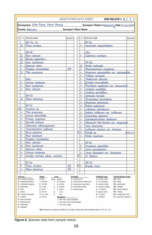
VEGETATION DATA SHEET DNR RELEVE # __ __ __ __

Surveyor(s): _________________________________________________Surveyor's Releve #: ___________Date: _________County: ___________________________________Surveyor's Place Name: ____________________________________

ID C.S SPECIES NAME REMARKS ID C.S SPECIES NAME REMARKS

. .

. .

. .

. .

. .

. .

. .

. .

. .

. .

. .

. .

. .

. .

. .

. .

. .

. .

. .

. .

. .

. .

. .

. .

. .

. .

. .

. .

. .

. .

. .

. .

. .

. .

. .

. .

. .

. .

. .

. .

Life Form Height Cover Sociability Reliability Code Selected Remark Codes B = broadleaf evergreen 8 >35m Group Species 5 = extensive mat 0 = variety certain DD = deadD = broadleaf deciduous 7 = 20-35m c 5 75-100% 4 = small colonies, broken mat 1 = cf. var./subsp. DY = dyingE = needleleaf evergreen 6 = 10-20m i 4 50-75% 3 = large group, many plants 2 = species certain GE = germinatingG = graminoids 5 = 5-10m p 3 25-50% 2 = small dense clumps 3 = species complex SD = seedlingH = forbs 4 = 2-5m r 2 5-25% 1 = growing singly 4 = cf. species SP = sprout (coppice)L = lichens 3 = 0.5-2m b 1-5% 5 = genus certain FR = fruitingM = mosses & liverworts 2 = 0.1- 0.5m a <1% 6 = cf. genus OP = outside plot (<2m)C = climbers 1 = 0-0.1m Abundance 7 = unknown ## = specimen collection #K = stem succulents 1 <5% cover, many individualsF = floating-leaved + <5% cover, few (2-20) individuals S = submerged r <5% cover, singleX = epiphytes

Note: indicate tree canopy by recording "Ca" to right of canopy layer life form/height code (ex: "D6 − 9p, Ca" )

9 1 7 1

24 Jul 2009Erika Rowe, Norm Aaseng ER240705 -2

Beltrami

E6-7p, Ca 3 Pinus strobus

D5-6i2 Acer rubrum2 Betula papyrifera2 Acer saccharumr Quercus rubrar Populus tremuloides OP2 Tilia americana

D4p+ Ostrya virginiana+ Acer saccharum+ Acer rubrum

E4-5r2 Abies balsamea

D1-3r+ Fraxinus sp.+ Tilia americana+ Cornus alternifolia+ Prunus virginiana+ Diervilla lonicerar Viburnum rafinesquianum+ Toxicodendron rydbergii+ Dirca palustris1 Acer spicatum+ Populus tremuloides1 Acer rubrum2 Acer saccharum+ Quercus rubra+ Ostrya virginiana+ Corylus cornuta subsp. cornuta

E1-2a1 Pinus strobus SD+ Abies balsamea SD

B1-2a+ Vaccinium angustifolium

C2ar Celastrus scandens

H1-2p2 Aralia nudicaulis1 Maianthemum canadense+ Anemone quinquefolia var. quinquefolia1 Trillium cernuum+ Thalictrum dioicum1 Eurybia macrophylla+ Pteridium aquilinum var. latiusculum+ Uvularia sessilifolia+ Uvularia grandiflora+ Clintonia borealis+ Streptopus lanceolatus+ Anemone americana+ Rubus pubescens+ Lathyrus ochroleucusr Galium triflorum var. triflorum+ Osmorhiza claytoniir Symphyotrichum ciliolatum+ Athyrium filix-femina var. angustumr Vicia americana+ Lathyrus venosus var. intonsus+ Pyrola sp ERR09-12r Aralia racemosa

G1-2r1 Oryzopsis asperifolia1 Carex pensylvanicar Carex deweyana var. deweyanar cf. Elymus

M1-1b+ Bryales moss

5

6

6

5

Figure 6. Species data from sample relevé.

26

species present. The basic procedure for recording plant data in a relevé is to divide the vegetation into layers based on the life-forms and heights of the plant species and then record the cover or abundance of each species within each life-form and height-class group. For example, in a forest, the vegetation often is divided into a tree canopy layer, a tree subcanopy layer, a shrub and tree sapling layer, a forb layer, and a graminoid layer (Fig. 8, page 29), and the species in each layer are recorded on the datasheet along with their cover or abundance.

In accord with the division of the vegetation in a relevé into groups by life-form and height, the vegetation and plant species data are recorded on the relevé form in blocks of data lines that belong to separate life-form and height-class, or physiognomic, groups. The first line of each group has a letter code designating the life-form of the plants, a number code or codes designating the height class range, and another letter code for the collective cover of the group. An example of a physiognomic group line is:

E 4–6 c

In this example, “E” is the life-form code for needleleaf evergreen plants, “4–6” is the range of height classes of the plants in the layer (which in this case is 2 meters to 20 meters), and “c” is a code for the estimated collective cover of the plants in the layer (in this case, 75–100%). See below for complete lists and definitions of the codes for life-form, height class, and coverage class for physiognomic groups.

The individual species records are written immediately below the physiog-nomic group line. Each species data record consists of a code indicating the reliability of the identification of the species, a code for the cover or abundance of the species within the height class of the group, (sometimes) a code for the distribution of the species within the plot, the species name, and (sometimes) codes describing the vegetative state of the species. An example of a typical physiognomic is given in Figure 7.




. .

. .

. .

. .

. .

. .

. .

. .

. .

. .

. .

. .

. .

. .

. .

. .

. .

. .

. .

. .

. .

. .

. .

. .

. .

. .

. .

. .

. .

. .

. .

. .

. .

. .

. .

. .

. .

. .

. .

. .



E4 - 6 c 1 Pinus strobus FR1 Abies balsamea DF, BR1 Picea cf. glauca #1

2 42 r4 +

Figure 7. Example of physiognomic group.

The first line of data in this example (“E 4–6 c”) gives the life-form, height classes, and cover of the group as a whole; subsequent lines are for the in-dividual species within the group. As an example, within the physiognomic group, Pinus strobus has been reliably identified to the level of species (ID = 2), has a total canopy cover of 50–75% (C = 4), is growing singly throughout the plot (S = 1), and is in fruit (FR). See below for complete lists and defini-tions of the codes for reliability of identification of species, species cover and

27

abundance, species distribution or sociability, and remarks about vegetative condition.

As illustrated above, the column headings on the relevé form refer only to the species data variables (reliability of i.d., cover, sociability, name, and remarks). The structural data codes (life-form, height classes, and physiognomic group cover) are entered in the “Species” column, and it is understood that these structural variables apply to all of the species in the rows immediately below that entry. Blank rows are used to separate the blocks of data lines for each physiognomic group. See Figure 6 (page 26) for examples of how physiog-nomic groups and species data are organized on the relevé form.

One potentially confusing aspect of doing relevés is determining the num-ber of separate physiognomic groups within each relevé. The total number of groups is determined by both the number of life forms represented in the plot and the number of distinct height layers for each life form. For example, a forest relevé containing plants of four different life forms (e.g., broad-leaved deciduous plants, needle-leaved coniferous plants, forbs, and graminoids) and three distinct height layers (e.g., canopy, subcanopy, and ground layer) would have at least four physiognomic groups, because each life-form is recorded in a separate group (for example, broad-leaved deciduous species and nee-dle-leaved coniferous species in the tree canopy layer are placed in separate tree canopy physiognomic groups). If each life form in the above relevé was present in all three height layers, the relevé would have twelve physiognomic groups, although in reality the number will be between four and eight because forbs and graminoids do not occur in canopy or subcanopy layers. Figure 8 illustrates how height classes and physiognomic groups might be delineated in a forested relevé with broad-leaved deciduous trees and shrubs, needle-leaved coniferous trees, forbs, and graminoids.

In general, the number of life forms in each relevé is determined by the plant species present and does not involve any interpretation by the surveyor. The number of height classes that are delineated in a relevé plot does involve in-terpretation of the structure of the vegetation by the surveyor and is not neces-sarily a pre-determined number based on the species present1. Therefore, the number of physiognomic groups in any relevé is dependent, to some extent, on the surveyor’s field interpretations.

Another sometimes confusing aspect of relevé species data is that it is com-mon for a species to be recorded in several different physiognomic groups if that species occurs in different height layers or, for a few species in Minnesota, if it exhibits more than one life form. For example, relevés in which sugar maple is present often have three species records for sugar maple–one in the tree canopy height class, one in the subcanopy height class, and one in the shrub layer height class.

1Most decisions made in stratifying vegetation into height classes involve tree and shrub species. For forested vegetation, woody species are often separated by surveyors into a seedling/shrub layer (sometimes the seedling layer is separated from the shrub layer), a subcanopy layer, and a canopy layer, while for woodland and savanna vegetation, in which a distinct subcanopy is likely to be absent, trees are often stratified into a seedling/shrub layer and a canopy layer. The overall goal in stratifying vegetation into height classes is not to record every visibly distinguishable layer in the stand but to provide a general impression of stand structure, with information that might be useful in interpreting regeneration and succession.

28

Figure 8. Delineation of height classes in forested relevé plot.

2m

0.5m

E6-7

D4

-5D1

-3H1

-2G1

-2}}

35m

10m

D6

-7

29

PHYSIOGNOMIC GROUP VARIABLESLife-Form Codes: The life-form of each physiognomic group is represented by a one-letter code. This code is the first character of the physiognomic group line and is capitalized to distinguish it from the code for the physiognomic group coverage class (see Coverage Classes below). The definitions and codes for life-forms used by the DNR follow Küchler (1967). Appendix K pro-vides a list of the life-forms for selected species in Minnesota whose life-forms are not obvious. A checklist of all vascular plant species in Minnesota with life-form (physiognomic) codes is available on the DNR’s website at www.mndnr.gov/eco/mcbs/plant_lists.html.

Woody PlantsB = Broadleaf Evergreen. This group of woody plants has broad leaves (as distinguished from needle-like leaves) that persist for two to several years. In Minnesota, this group is most often represented by members of the Eri-caceae (Andromeda, Arctostaphylos, Chamaedaphne, Epigaea, Gaultheria, Kalmia, and the cranberry and lingonberry species in the Vaccinium genus). Also included are the non-ericaceous species Chimaphila umbellata, Hud-sonia tomentosa, Empetrum atropurpureum, and E. nigrum.

D = Broadleaf Deciduous. This group of woody plants has broad leaves that are either shed annually or are dead (non-photosynthetic) during some part of the year. In Minnesota this group encompasses many tree and shrub genera (e.g., Acer, Betula, Corylus, Fraxinus, Quercus, Ulmus, etc.).

E = Needleleaf Evergreen. This group of woody plants includes both nee-dle-leaved and scale-leaved evergreens, which in Minnesota are all gym-nosperms. The needle-leaved evergreen genera are Abies, Picea, Pinus, Taxus, and Tsuga; the scale-leaved genera are Juniperus and Thuja. By convention, Larix, the only needle-leaved deciduous genus in Minnesota, is currently placed in the needleleaf evergreen (E) group, although in the past it was separated into a needleleaf deciduous (N) group.

Herbaceous PlantsG = Graminoids. This group of herbaceous plants includes most plants that appear grass-like because of their long, linear leaves and unbranched form. In Minnesota, all members of the Cyperaceae, Juncaceae, and Poa-ceae are considered graminoids. Note: Typha species, although grass-like in form, are considered forbs. See Appendix K for a listing of other forb spe-cies in Minnesota that are grass-like in form.

H = Forbs. This group of herbaceous plants has broad leaves and is repre-sented in Minnesota by many angiosperm families. By convention, ferns and fern allies are grouped with forbs.

L = Lichens. This group includes all lichens that grow on the ground (either on soil or bare rock). In Minnesota the lichen genera Cladonia and Parmelia are examples of ground-covering taxa. Epiphytic lichens are included in the epiphyte special life-form (see below).

M = Mosses and Liverworts. This group includes all mosses that grow on the ground (either on soil or bare rock). In Minnesota the moss gen-era Brachythecium, Hylocomnium, Mnium, Pleurozium, Polytrichum, Ptilium,

30

and Sphagnum are examples of ground-covering taxa. Epiphytic mosses are included in the epiphyte special life-form (see below).

Special Life-FormsC = Climbers. This group includes all woody plants that are rooted in the ground and climb objects or other plants. In Minnesota this group is most often represented by the genera Rhus, Parthenocissus, and Vitis. Herba-ceous climbers, such as those in the genera Convolvulus, Cuscuta, Di-oscorea, Lathyrus, and Vicia, are categorized as forbs.

K = Stem Succulents. In Minnesota this group includes only the native cacti genera, Escobaria and Opuntia. Plants with fleshy leaves, such as species of Sedum, are categorized as forbs.

X = Epiphytes. Epiphytes include a wide variety of plants that are not nec-essarily similar in growth form or appearance. By convention, this group in-cludes all plants that live on the above-ground parts of other plants. Among these are all epiphytic mosses and lichens and the parasitic vascular plant Archeuthobium pusillum. Parasitic plants that are apparently rooted in the soil, such as species of Monotropa and Orobanche, are categorized as forbs.

F = Floating-Leaved Aquatics. This group consists of floating-leaved aquatic species, including free-floating species such as Lemna trisulca and Spirodela polyrrhiza, and rooted species such as Brasenia schreberi, Nuphar variegata, and Nymphaea odorata.

S = Submerged Aquatics. This group consists of submerged aquatic spe-cies, including submerged species that have flowering parts extending above the water surface, such as Myriophyllum sibiricum and Utricularia vulgaris.

Height Class Codes: The heights of the plants in each physiognomic group are represented by numbers ranging from one to eight. These numbers are written after the life-form code in the physiognomic group line. The codes and definitions for height classes follow Küchler (1967) (Table 7).

If all of the plants in a physiognomic group fall within one height class, a single height-class code is used. For example, if a forest has a continuous canopy of deciduous trees that is between 10 and 20 meters in height, the physiognomic group line would be “D 6–6 c.” (In this example, the height class “6” is written twice as a reminder to data entry personnel that both allotted fields for height class in a species record need to be filled in the DNR’s relevé entry program; the line would have the same meaning if it was written “D 6 c.”)

If the plants of a given life-form are not strongly stratified or occupy more than one height class, a range of contiguous height classes is entered. For example, if the tree canopy in the above forest ranged from 10 to greater than 35 meters, the physiognomic group line would be “D 6–8 c.” When a range of height classes is given, it implies that the heights of the individual plants are evenly distributed between the lowest range value (in this case 10 meters) and the highest range value (in this case greater than 35 meters). If just a few of the trees in the above example were taller than 35 meters and the rest were

31

between 10 and 35 meters, then it would be appropriate to record the trees in two physiog-nomic groups (i.e., D 8–8 and D 6–7).

One aspect of identifying height classes that merits closer attention is the method of de-lineating height classes for canopy trees in a forest relevé. Some surveyors delineate the canopy tree layer as ranging from the tops of the shortest canopy trees to the tops of the tall-est canopy trees. This method tends to provide insight into stand history by emphasizing co-horts of trees and clearly separating trees in the canopy from younger trees in the under-story. Other surveyors delineate the canopy as ranging from the lower parts of the crowns of

the canopy trees to the tops of the canopy trees. This method tends to provide insight into vegetation structure and ecological function.

Tree Canopy Code: The physiognomic groups for canopy tree species in for-est, woodland, or savanna communities are given an additional label (“Ca”) to document that the group forms the tree canopy or part of the canopy. Re-cording the tree canopy code for physiognomic groups reduces ambiguity in assigning tree species to the canopy layers when analyzing relevé data. The tree canopy code is entered to the right of relevant physiognomic group line or lines (Fig. 9).

Coverage Class Codes: Coverage class codes are one-letter codes that rep-resent the estimated cover of all of the plants in a given physiognomic group. Cover is defined as the percent of the relevé plot that would be covered by the downward vertical projection of the leaf surface area. Coverage class codes are recorded after the height class codes in the physiognomic group line and are written in lowercase letters to distinguish them from the life-form codes.

The cover class codes and definitions follow Küchler (1967):

c = Continuous, with 75–100% cover. Continuous implies that the cover is distributed evenly across the relevé plot with plant canopies touching and to-tal projected cover exceeding 75%. For some sparsely leaved species, such as needleleaf evergreens and graminoids, the plant canopies may touch, yet not have greater than 75% coverage—these still are designated as hav-ing continuous cover.

32

height class meters

8 = > 35 7 = 20 - 35 6 = 10 - 20 5 = 5 - 10 4 = 2 - 5 3 = 0.5 - 2 2 = 0.1 - 0.51 = 0 - 0.1

Table 7. Height class codes.

Figure 9. Example of physiognomic group labeled as tree canopy.




. .

. .

. .

. .

. .

. .

. .

. .

. .

. .

. .

. .

. .

. .

. .

. .

. .

. .

. .

. .

. .

. .

. .

. .

. .

. .

. .

. .

. .

. .

. .

. .

. .

. .

. .

. .

. .

. .

. .

. .



E4 - 6 c, Ca 1 Pinus strobus FR1 Abies balsamea DF, BR1 Picea cf. glauca #1

2 42 r4 +

i = Interrupted, with 50–75% cover. This class is generally assigned to strata with a hole in otherwise continuous coverage, to strata in which the plant canopies do not touch, or to strongly clumped herbaceous or grami-noid species where the canopies of the individual clumps do not touch.

p = Park-like or in patches, with 25–50% cover. This class is most often assigned to tree or shrub strata where the plants occur in patches, or to patchy colonies of herbaceous plants.

r = Rare, with 5–25% cover. This class applies to strata in which the plants are more widely scattered than in “p.” Often, the distinction between “p” and “r” is to separate strata composed primarily of plants with vegetatively re-producing colonies from strata composed of plants reproducing by long rhi-zomes or seeds.

b = Barren or barely present, with 1–5% cover. This is generally assigned to strata with plants that have fairly large leaf areas (such as bracken fern) but are widely scattered in the plot.

a = Almost absent, with <1% cover. This class is assigned to strata with plants that have small leaf areas (such as graminoids and conifer seedlings) and are widely scattered.

SPECIES OCCURRENCE DATA VARIABLESSpecies Names: Species names are recorded on the relevé form in the lines below the associated physiognomic group line, using the Latin name for the species. The nomenclature used by the DNR is based on the published volumes of Flora of North America North of Mexico (Flora of North America Editorial Committee 1993– ). For species not yet published in Flora of North America, nomenclature is based on Manual of Vascular Plants of Northeast-ern United States and Adjacent Canada (Gleason and Cronquist 1991). There are a few exceptions to this convention for some woody species and some rare species. The DNR’s official checklist of names for the vascular plant species that have been documented in Minnesota is available at www.mndnr.gov/eco/mcbs/plant_lists.html.

The surveyor records as much of the species name on the relevé form as is warranted by their confidence in the identity of the plant (e.g., Solidago sp., Solidago nemoralis, Solidago nemoralis ssp. decemflora, etc.). It is good prac-tice to write the full binomial name of a species on the relevé form whenever a plant has been reliably identified to species, even if there is only one species of the genus in Minnesota; if data entry personnel are not familiar with a par-ticular species they are likely to enter the species record exactly as it appears on the relevé form. (For example, if a surveyor recorded only “Amphicarpaea” on the relevé form, it is possible that the plant would be entered in the DNR’s relevé database only to the level of the genus, even though there is only one species of Amphicarpaea in Minnesota (i.e., A. bracteata).) It is conventional to record dead individuals of canopy tree species separately from live individu-als of the same species. Species record lines for dead specimens are denoted by entering the code “DD” in the Remarks field (see Remark Codes below).

33

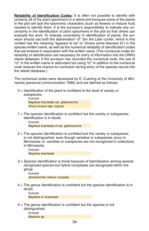
Reliability of Identification Codes: It is often not possible to identify with certainty all of the plant specimens in a relevé plot because some of the plants in the plot will lack the taxonomic characters (such as flowers or mature fruit) needed to identify them. It is the surveyor’s responsibility to indicate any un-certainty in the identification of plant specimens in the plot so that others can evaluate the work. To indicate uncertainty in identification of plants, the sur-veyor should use both the abbreviation “cf.” (for the Latin confer, which in this context has the meaning “appears to be” or “shows some likeness to”) in the species written name, as well as the numerical reliability of identification codes that are entered in association with the written name. (The numerical codes for reliability of identification are necessary for entry of information into the DNR’s relevé database. If the surveyor has recorded the numerical code, the use of “cf.” in the written name is redundant but using “cf.” in addition to the numerical code reduces the chance for confusion during entry of the species record into the relevé database.)

The numerical codes were developed by E. Cushing at the University of Min-nesota (personal communication 1986) and are defined as follows:

0 = Identification of the plant is confident to the level of variety or subspecies.

Example Baptisia bracteata var. glabrescens Alnus incana ssp. rugosa

1 = The species identification is confident but the variety or subspecies identification is in doubt.

Example Baptisia bracteata cf.var. glabrescens

2 = The species identification is confident but the variety or subspecies is not distinguished, even though varieties or subspecies occur in Minnesota; or, varieties or subspecies are not recognized in collections in Minnesota.

Example Baptisia bracteata

3 = Species identification is trivial because of hybridization among several recognized species but hybrid complexes are recognized within the group.

Example Amelanchier interior complex

4 = The genus identification is confident but the species identification is in doubt.

Example Baptisia cf. bracteata

5 = The genus identification is confident but the species is not distinguished.

Example Baptisia sp.

34

6 = The genus identification is in doubt. Example cf. Baptisia sp.

7 = The plant is unknown but only one species is probably included.Plants recorded as “unknown” should be collected for later identification (unless the surveyor knows from experience that the specimen does not have the developed taxonomic characters necessary for identification) and the collection number entered in one of the remarks fields in the species data line.

In practice, the majority of species records on any given relevé are assigned a reliability of “2.” Therefore, in order to save time when recording species data on the relevé data sheet, it is common practice for surveyors to record reliabil-ity of identification codes only when they differ from “2.” If this is the convention used, the surveyor should indicate clearly that the code is “2” unless otherwise marked.

Cover/Abundance Codes: The DNR uses the Braun-Blanquet cover/abun-dance scale to designate the cover or abundance of each plant species within a given physiognomic group or layer. The categories in this scale are recorded on the relevé form using codes that include numbers (1 to 5) and characters (“+” and “r”). The numbers 2, 3, 4, and 5 designate cover classes for species with 5% to 100% cover in the physiognomic group. The convention for esti-mating species cover is to sum the “canopy cover” of each individual of the species in the layer. (Canopy cover is defined as the percentage of the ground covered by the downward projection of the outermost perimeter of the spread of foliage of each plant. This is in contrast to “foliar cover,” which is defined as the percentage of the ground covered by the downward projection of stem and leaf area, exclusive of gaps between stems and leaves [Society for Range Management 1989; Jennings et al. 2004].) The codes 1, +, and r designate qualitative estimates of the abundance (number) of plants of a species with less than 5% cover in a physiognomic group. See Mueller-Dombois and El-lenberg (1974) or McCune and Grace (2002) for discussions of the Braun-Blanquet cover/abundance scale and similar scales.

The use of both cover and abundance classes is intended to enable the re-cording of meaningful data from one relatively large plot for both large, cover-forming plants and small plants that seldom cover much of the plot. For exam-ple, if one used a pure cover scale there are many species that would almost always be assigned the lowest cover value because even when numerous in a relevé plot they tend to cover very little of the plot area. This is true for many diminutive forb and graminoid species. On the other hand, if one used a scale with classes based only on abundance, the importance of canopy trees would be diminished relative to that of herbaceous species because canopy trees typically have few individuals within a plot, even when the leaf area of a spe-cies may effectively cover the entire plot. Other sampling methods overcome the need for a split cover/abundance scale by using large plots to sample larger, cover-forming plants (such as trees and shrubs), and small plots nested within the large plots for sampling herbaceous plants.

35

One convention used by the DNR is that whenever the cover of a plant is greater than 5% in the plot, cover takes precedence over abundance. For ex-ample, if there is a single individual of a tree species in the canopy in a plot, but that individual has a leaf area that covers 30% of the plot, the species would be given a “3” for cover/abundance rather than an “r.” If, however, there was a single individual with leaf area covering less than 5% of the plot, that species would be given an “r” for cover/abundance. The same holds for canopy trees whose stems fall outside the plot but whose leaf area covers a portion of the relevé plot. If the leaf area covers more than 5% of the plot, the species is given the appropriate cover value (i.e., 2, 3, 4, or 5). If the leaf area covers less than 5% of the plot, the species is given an abundance value of “r,” and “OP” is recorded in the Remarks column to indicate that the stem is outside the plot. It is useful for surveyors to keep in mind that when conducting visual estimates of species cover there is a tendency for observers to overestimate cover of large species, species in flower or clumped in distribution, and spe-cies that are known, and to underestimate cover of small species, species in vegetative state, species distributed evenly in the plot, and species not known to the observer (Kershaw 1973, Kent and Coker 1992).

The Braun-Blanquet cover/abundance scale (after Mueller-Dombois and El-lenberg 1974) is as follows:

5 = 75%–100% (Cover code.) Assigned to a species within a particular physiognomic group when that species’ cover is between 75% and 100% of the relevé plot area.

4 = 50%–75% (Cover code.) Assigned to a species within a physiog-nomic group when that species’ cover is between 50% and 75% of the relevé plot area.



1 = < 5% (Abundance code.) Assigned to a species within a physi-ognomic group when there are numerous individuals of the species, but those individuals collectively cover less than 5% of the relevé plot area.

+ = < 5% (Abundance code.) Assigned to a species within a physi-ognomic group when there are only a few (approximately 2–20) individuals of the species and those individuals collectively cover less than 5% of the relevé plot area.

r = < 5% (Abundance code.) Assigned to a species within a physi-ognomic group when there is only a single individual of the species (a plant with two stems arising from the same

36

root would be classified as a single individual). This code is also assigned to species that fall just outside the relevé plot (no matter how numerous they are outside the plot). For species that are assigned an abundance code of “r” because they fall outside the plot, the surveyor also en-ters “OP” in the Remarks column. The recording of spe-cies that are outside the plot is meant to alert others that these species are present in the stand, but happened not to fall in the relevé plot. The convention for species out-side of the plot is to record only those species that are representative of the stand (rather than of anomalous mi-crohabitats within the stand) and that are within 2 meters of the plot boundary.

A useful approach for estimating species cover when applying the Braun-Blan-quet scale is to decide first if the species covers more or less than 50% of the relevé plot. If it covers more than 50%, then the surveyor is left to determine if the coverage is 50–75% or 75–100%. If the cover is less than 50%, then the surveyor next determines whether the cover is 25–50% or less than 25%. If less than 25%, then the surveyor determines whether it is 5–25% or less than 5%. If less than 5%, the species is assigned one of the three abundance val-ues. Note that the sum of the cover values for species in a physiognomic group should be consistent with the cover assigned to the physiognomic group as a whole. For example, if in a given relevé there are three tree species in the D 6–7 layer and each of the species is assigned a value of “+,” with less than 5% cover, then the D 6–7 layer as a whole should not be assigned cover greater than “R” (= 5–25%).

Sociability Codes: (Optional) Sociability codes describe how a species is distributed within the relevé plot. They are only rarely recorded by DNR survey-ors as they do not contribute useable information for classification analyses. When recorded, sociability codes refer only to the distribution of a species as it occurs in a particular physiognomic group. For example, it often hap-pens that the distribution of a tree species is uniform within the tree stratum and clumped within the seedling stratum. The codes for sociability are (after Mueller-Dombois and Ellenberg 1974):

5 = Assigned to species where the plants are growing in a large, essen-tially monotypic stand or swarm that forms an extensive mat. This code typically is applied to non-woody plants (for example, moss or lichen carpets, graminoid sods, etc.)

4 = Assigned to species where the plants are growing in small colonies or broken mats. This code typically is applied to non-woody plants (for example, broken moss or lichen carpets and also colonies of herbaceous plants that have enlarged to the point where they are beginning to coalesce).

3 = Assigned to species where the plants are growing in small patches or in cushions. This code typically is applied to small isolated clones of herbaceous plants, patches of shrubs, and moss or lichen colonies.

37

2 = Assigned to species where the plants form small, often dense clumps. These small clumps may be rather evenly dispersed within the relevé. This code is often applied to woody or herbaceous plants where several aerial stems originate from the rootstock of a single genet.

1 = Assigned to species growing solitarily. This code is applied to both woody and herbaceous plants with single stems that appear to be evenly dispersed within the relevé plot.

Remark Codes: Remark codes are two-character codes that indicate some special attribute of the species as it occurs in a physiognomic group. Some remark codes refer to the species’ viability (that is, they are qualitative esti-mates of the ability of the species to perpetuate itself). Other remark codes refer to the condition of the species as affected either by inherent factors (such as seasonal phenology or life-cycle) or external factors (such as herbivory, windthrow, or fire). When a vitality code is used, it is good practice to either enter an associated condition code that helps to explain the vitality of the species, or to include an explanatory note in the Remarks or Notes fields on the first side of the relevé form. For example, if the vitality code “PV” (indicat-ing poor vitality) is applied to a species record, then one would also apply a condition code to that species record to indicate why it had poor vitality (for example, it may have been defoliated by insects, in which case one would also enter the condition code “DF” for “defoliated” in the remark code column). The list of potential remark codes is not strictly limited, and miscellaneous remarks pertaining to features other than vitality or condition may be created to suit particular vegetation studies. Some commonly used standard remark codes are listed in Table 8.

Table 8. Standard codes for plant species remarks.

VitalityDD = dead LU = luxurious growth

DY = dying PV = poor vitality

EX = being driven out

ConditionBU = budding MS = multiple stemmed

BR = browsed MW = mowed

DF = defoliated OG = open grown

FL = flowering PF = past fruiting

FR = fruiting SE = present as seed

FS = fire scarred ST = sterile

GE = germinating SD = seedling

GR = grazed SP = sprout (coppice)

MiscellaneousIN = introduced in Minnesota OP = just outside plot (< 2 meters)RA = rare in Minnesota ## = specimen collection number

38

Appendix A. Contributing Samples to the DNR Relevé Database

Most relevé samples are contributed to the DNR’s Relevé Database by provid-ing the DNR with paper copies of the relevés. For studies involving large num-bers of relevés, the contributor should contact the DNR to determine whether it would be more efficient to arrange some other method of submission. For further guidance on submitting relevés to the DNR’s Relevé Database, please contact: Norm AasengMinnesota Biological SurveyMinnesota Department of Natural Resources500 Lafayette Road, Box 25St. Paul, Minnesota 55155(651) [email protected]

Appendix B. Obtaining Data from the DNR Relevé Database

Electronic datasets or paper copies of relevés housed in the DNR’s Relevé Database are available to researchers interested in vegetation study. For infor-mation on obtaining relevé datasets or printouts, please contact:

Daniel WovchaMinnesota Biological SurveyMinnesota Department of Natural Resources500 Lafayette Road, Box 25St. Paul, Minnesota 55155(651) [email protected]

Appendix C. Obtaining a Copy of the DNR Relevé Field Form

A printable version of the DNR relevé field form is available on the DNR’s web-site at www.mndnr.gov/eco/mcbs/vegetation_sampling.html.

A paper copy of the field form can be obtained by contacting:

Daniel WovchaMinnesota Biological SurveyMinnesota Department of Natural Resources500 Lafayette Road, Box 25St. Paul, Minnesota 55155(651) [email protected]

39

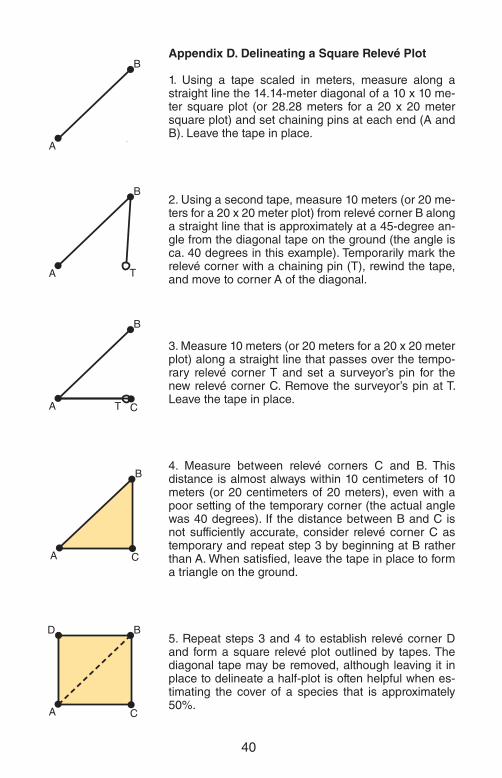
Appendix D. Delineating a Square Relevé Plot

1. Using a tape scaled in meters, measure along a straight line the 14.14-meter diagonal of a 10 x 10 me-ter square plot (or 28.28 meters for a 20 x 20 meter square plot) and set chaining pins at each end (A and B). Leave the tape in place.

B

A

2. Using a second tape, measure 10 meters (or 20 me-ters for a 20 x 20 meter plot) from relevé corner B along a straight line that is approximately at a 45-degree an-gle from the diagonal tape on the ground (the angle is ca. 40 degrees in this example). Temporarily mark the relevé corner with a chaining pin (T), rewind the tape, and move to corner A of the diagonal.

B

A T

3. Measure 10 meters (or 20 meters for a 20 x 20 meter plot) along a straight line that passes over the tempo-rary relevé corner T and set a surveyor’s pin for the new relevé corner C. Remove the surveyor’s pin at T. Leave the tape in place.

B

A CT

4. Measure between relevé corners C and B. This distance is almost always within 10 centimeters of 10 meters (or 20 centimeters of 20 meters), even with a poor setting of the temporary corner (the actual angle was 40 degrees). If the distance between B and C is not sufficiently accurate, consider relevé corner C as temporary and repeat step 3 by beginning at B rather than A. When satisfied, leave the tape in place to form a triangle on the ground.

B

A C

5. Repeat steps 3 and 4 to establish relevé corner D and form a square relevé plot outlined by tapes. The diagonal tape may be removed, although leaving it in place to delineate a half-plot is often helpful when es-timating the cover of a species that is approximately 50%.

B

A C

D

40

Appendix E. List of InstitutionsConsultantEnvironmental Quality Board–Copper Nickel StudyMinnesota Pollution Control AgencyMNDNR Ecological and Water ResourcesMNDNR Ecological Land Classification ProgramMNDNR Minnesota Biological SurveyMNDNR Natural Heritage ProgramMNDNR Parks and TrailsMNDNR Scientific & Natural Areas ProgramMNDNR WildlifeNational Park ServiceNatural Resource Conservation ServiceNatural Resources Research Institute–UMDThe Nature ConservancyUniversity of MinnesotaU.S. Forest Service–Superior National ForestU.S. Forest Service–Chippewa National ForestWhite Earth NationWisconsin DNROther Appendix F. List of OwnershipsBureau of Land Management Colleges (Other) County (Other) County (Park) County (Tax Forfeit & Forest Land) Local (Park) Local Government MN Department of Agriculture MN Department of Military Affairs MN Department of Transportation MN DNR Ecological and Water Resources (Scientific & Natural Areas) MN DNR Enforcement MN DNR Fisheries MN DNR Forestry MN DNR Minerals MN DNR Parks and Trails MN DNR Wildlife MN State Historical Society National Park Service (National Monument) National Park Service (National Wild and Scenic River) National Park Service (Voyageurs National Park) Native Institution Non-Profit Organization Private (Corporation) Private (Individual) State of Minnesota (Other) The Nature Conservancy U.S. (Other Federal Lands) U.S. Army Corps of Engineers U.S. Fish and Wildlife Service (National Wildlife Refuge)U.S. Fish and Wildlife Service (Waterfowl Production Area) U.S. Forest Service (Boundary Waters Canoe Area)U.S. Forest Service (National Forest)University of Minnesota UnknownWatershed District

41

Appendix G. Invasive Earthworm Rapid Assessment

Dichotomous key for 5-stage rapid classification of earthworm invasion in deciduous and mixed deciduous-coniferous forests (from Loss et al. 2013) 1. Leaf litter greater than one year present (Oi and Oe layers present). 1a. Yes (go to 2) 1b. No, leaf litter (Oi) from previous autumn only (go to 6)

2. Small, fragmented, relatively un-decomposed leaves greater than one year present. 2a. Yes, Oe present (go to 3) 2b. No, leaf litter (Oi) from previous autumn only (go to 6)

3. Intact, layered forest floor, leaves bleached and stuck together, Oi , Oe, and Oa layers present, fine plant roots in humus (Oa) and leaf fragments (Oe), no earthworms, castings, or middens present. 3a. Yes (Stage 1 – potentially earthworm-free) 3b. No (go to 4)

4. Layered forest floor, but leaves loose, Oi, Oe, and patches of Oa layers present. Some small earthworms and/or earthworm castings present in humus (Oa), fine plant roots present. 4a. Yes (Stage 2) 4b. No (go to 5)

5. Leaf litter (Oi) from previous autumn and small fragmented leaves (Oe) under intact leaves present, no humus (Oa), mineral soil (A horizon) present, earthworm castings present (≤50% of forest floor/mineral soil interface covered), fine plant roots absent. 5a. Yes (Stage 3) 5b. No (go to 6)

6. Leaf litter (Oi) from previous autumn present, mineral soil (A horizon) present, earthworm castings abundant (>50% of forest floor/mineral soil interface covered), fine plant roots absent, middens absent or present (≤9 middens in 5-m radius). 6a. Yes (Stage 4) 6b. No (go to 7)

7. No forest floor (Oi or Oe), humus (Oa) or fragmented leaves present, mineral soil (A horizon) present, earthworm castings abundant (>50% of forest floor/mineral soil interface covered), middens abundant (>9 middens in 5-m radius). 7a. Yes (Stage 5)

42

Appendix G. Invasive Earthworm Rapid Assessment (cont.)

Definitions1 Forest Floor (O Horizon) = layer of fresh and decaying organic material (leaves, needles, twigs, etc.) at the ground surface. May be separated into three layers: Oi, Oe, and Oa (all three are not always present).

Oi = litter layer composed of intact leaves from the previous fall. Leaves often complete or nearly complete, readily distinguishable and even identifiable to species. Often layered or matted.

Oe = litter layer of fragmented leaves just below Oi layer, consisting of leaves greater than one year old that are relatively undecomposed but fragmented so they are difficult to identify to species. Peat-like and generally not blackened in color.

Oa = humus layer, consisting of decomposed organic material mixed with min-eral soil (mineral soil content is less than 50% as estimated by visual inspec-tion). May be very black and mixed with worm cast material, but still maintains network of fine roots (dead or alive) and recognizable organic material.

Mineral Soil or Top Soil (A Horizon) = soil horizon just below the O horizon (or if there is no O horizon, this horizon forms the surface horizon). Characterized by an accumulation of humified organic matter mixed with mineral material and composed of more than 50% mineral soil relative to organic matter. Some-times the organic component is difficult to see, but is indicated by a black or dark brown color due to the accumulation of soluble organic molecules. Where earthworms are abundant this layer may be completely composed of worm cast material. In worm-free conditions this layer may not be present; rather, a leached, lighter-colored sandy or silty mineral horizon (E horizon) with mea-surably less organic material begins immediately below the O horizon.

Middens = distinctive piles of cast material around the openings of earthworm burrows. These middens are usually about 1–5cm in diameter and 1–3cm in height, with a burrow hole (2–4mm in diameter) near the center. The burrow entrances of middens also often have large numbers of leaf petioles or frag-ments of leaves sticking out of them. These become stuck as the inhabitants attempt to pull leaves into burrows.

1 Great Lakes Worm Watch. Invasive earthworm rapid assessment tool. Natural Resources Research Institute, University of Minnesota Duluth. http://greatlakeswormwatch.org

43

Midden

Appendix G. Invasive Earthworm Rapid Assessment (cont.)

Castings = material cast by earthworms on the surface of the soil. Earthworm castings are composed of smooth and rounded clumps of soil, which distin-guish them from the rougher, angular or crumb-like surface of soil aggregates that have not been worked by earthworms. Cast material is also usually very dark brown or black in color.

Soil aggregates that have been reworked by earthworms

Soil aggregates that have not been reworked by earthworms

44

Very Poor

Poor

Well

SomewhatExcessive

Excessive

SomewhatPoor

ModeratelyWell

45

Footnotes1 Exclude mottles that are faint or few in number2 Exclude gray “E” horizons3 Loamy textures: sandy loam, silty loam, loam, clay loam, sandy clay loam, silty clay loam, silty clay, and sandy clay Clayey textures: clay, silt4 Sandy textures: sand, loamy sand

StartGray mottles1 or matrix2 within 25cm of

the mineral soil surface.

Gray mottles or matrix 25–50cm below

surface.

Gray mottles or matrix50-100cm below surface.

> 20cm organicsoil (i.e., peat).

< 20cm organicsoil (i.e., peat).

no

no

noyes

yes

yes

yes

yes

Appendix H. Key to Soil Drainage Classes

nono

>35% gravel by volume.

yesLoamy or clayey3 layers present within 150cm of

surface.

Sandy texture4 present throughout the upper 150cm; no loamy or

clayey layers.

no

yes

yes

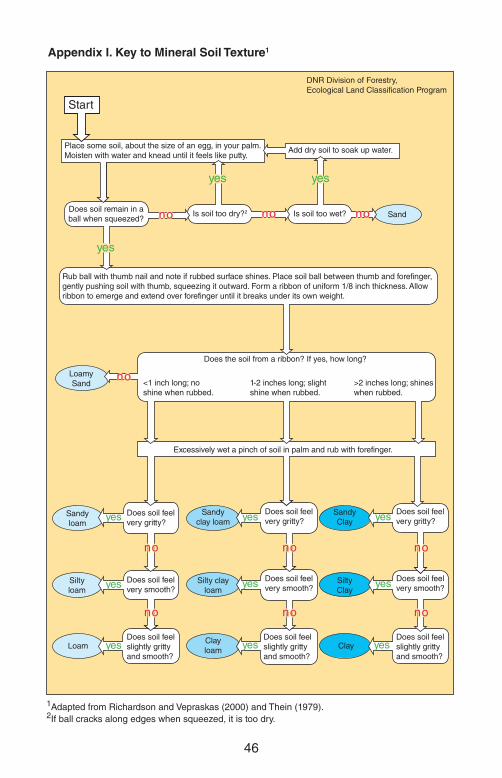
Sandyclay loam

Sandy loam

Siltyloam

Loam

Does soil feelvery gritty?

Does soil feelvery smooth?

Does soil feel slightly grittyand smooth?

yes

yes

no

no

yes

46

SandyClay

Clay loam

Appendix I. Key to Mineral Soil Texture1

1Adapted from Richardson and Vepraskas (2000) and Thein (1979).2If ball cracks along edges when squeezed, it is too dry.

DNR Division of Forestry,Ecological Land Classification Program


Loamy Sand

Silty clay loam

SiltyClay

Clay


Place some soil, about the size of an egg, in your palm.Moisten with water and knead until it feels like putty.

Add dry soil to soak up water.

Start

Sand



1-2 inches long; slightshine when rubbed.

Does the soil from a ribbon? If yes, how long?

<1 inch long; no shine when rubbed.

>2 inches long; shineswhen rubbed.

Excessively wet a pinch of soil in palm and rub with forefinger.

Rub ball with thumb nail and note if rubbed surface shines. Place soil ball between thumb and forefinger, gently pushing soil with thumb, squeezing it outward. Form a ribbon of uniform 1/8 inch thickness. Allow ribbon to emerge and extend over forefinger until it breaks under its own weight.

Does soil remain in a ball when squeezed?

Is soil too dry?2 Is soil too wet?



yes

yes

no

yes

yes

yes

yes

yes

no no

yesyes

no

no

no

no

no

47

Text

ure

Cla

ss

Val

ue o

n V

on P

ost p

eat

deco

mpo

sitio

n sc

ale1

Col

or o

f org

anic

mat

eria

l

Dec

ompo

sitio

n st

ate

of p

lant

mat

eria

l

Col

or o

f wat

er r

elea

sed

whe

nm

ater

ial i

s sq

ueez

ed

Am

ount

of o

rgan

ic m

ater

ial

that

esc

apes

bet

wee

nfin

gers

whe

n sq

ueez

ed

H4

to H

6H

1 to

H3

At l

east

one

-hal

f.U

p to

one

-thi

rd.

Non

e.

Ver

y da

rk, a

lmos

t pas

ty(if

any

is r

elea

sed)

.V

ery

mud

dy a

nd d

ark.

Cle

ar to

mud

dy b

row

n.

Ver

y da

rk g

rey

to b

lack

.D

ark

redd

ish

brow

n to

dar

k gr

eyis

h br

own.

Ligh

t yel

low

ish

brow

n or

re

ddis

h br

own.

Com

pose

d of

sap

ric

orga

nic

mat

eria

l, in

whi

ch p

lant

re

mai

ns a

re v

ery

high

ly

deco

mpo

sed

to c

ompl

etel

y de

com

pose

d. P

lant

rem

ains

ar

e in

desc

erni

ble

or r

educ

ed

to r

esid

ues

such

as

root

s an

d fib

ers.

Com

pose

d of

hem

ic

orga

nic

mat

eria

l, in

whi

ch

plan

t rem

ains

are

slig

htly

de

com

pose

d to

mod

erat

ely

deco

mpo

sed.

Pla

nt r

emai

ns

have

lost

som

e id

entif

iabl

e fe

atur

es a

nd s

ome

muc

ky.

amor

phuo

us m

ater

ial i

s pr

esen

t.

Com

pose

d of

fib

ric

orga

nic

mat

eria

l, in

whi

ch p

lant

re

mai

ns a

re u

ndec

ompo

sed

or v

ery

slig

htly

dec

ompo

sed.

M

ost p

lant

rem

ains

are

id

entif

iabl

e an

d no

am

orph

ous

mat

eria

l is

pres

ent.

Muc

kM

ucky

P

eat

Pea

t

1An English-language version and brief explanation of the Von Post scale of peat decomposition is presented in Andriesse (1988).

H7

to H

10

Appendix J. Characteristics of Wetland Organic Soils

Appendix K. Plant Species Commonly Assigned Incorrect Life-form Codes (based on analysis of relevés in DNR Relevé Database).

Woody Broadleaf Evergreens*Bog rosemary (Andromeda glaucophylla) B DBearberry (Arctostaphylos uva-ursi) B DLeatherleaf (Chamaedaphne calyculata) B DPipsissewa (Chimaphila umbellata) B DTrailing arbutus (Epigaea repens) B DCreeping snowberry (Gaultheria hispidula) B DWintergreen (Gaultheria procumbens) B DBeach heather (Hudsonia tomentosa) B DBog laurel (Kalmia polifolia) B DLabrador tea (Ledum groenlandicum) B DLarge cranberry (Vaccinium macrocarpon) B DSmall cranberry (Vaccinium oxycoccos) B DLingonberry (Vaccinium vitis-idaea) B D

Woody Climbing Plants*Climbing bittersweet (Celastrus scandens) C DWild honeysuckle (Lonicera dioica) C DGrape honeysuckle (Lonicera reticulata) C DCanada moonseed (Menispermum canadense) C DVirginia creeper (Parthenocissus spp.) C DGreenbrier (Smilax tamnoides) C DVitis spp. C D

Woody Broadleaf Deciduous ShrubsSweet fern (Comptonia peregrina) D BFly honeysuckle (Lonicera canadensis) D CHairy honeysuckle (Lonicera hirsuta) D CRubus spp. (except R. pubescens and R. acaulis) D H

Woody Needeleaf EvergreensTamarack (Larix laricina) E D

GraminoidsTwig rush (Cladium mariscoides) G H

Evergreen ForbsGoldthread (Coptis trifolia) H BBunchberry (Cornus canadensis) H BTwinflower (Linnaea borealis) H BPartridgeberry (Mitchella repens) H BPyrola spp. H B

Climbing ForbsClematis spp. H CDodder (Cuscuta spp.) H CCommon hops (Humulus lupulus) H CFringed false buckwheat (Polygonum cilinode) H CBur cucumber (Sicyos angulatus) H CSmilax spp. (except S. hispida) H C

Graminoid-like ForbsScheuchzeria (Scheuchzeria palustris) H GTypha spp. H G

Moss-Like ForbsLycopodium spp. H LRock spikemoss (Selaginella rupestris) H L

Non-Woody Rubus SpeciesArctic raspberry (Rubus acaulis) H DDwarf raspberry (Rubus pubescens) H D

correct code

incorrect code

*List includes all species with this life-form in Minnesota.

48

References

Almendinger, J.C. 1985. The late-Holocene development of jack pine forests on outwash plains, north-central Minnesota. PhD diss., University of Minne-sota.

Almendinger, J.C. 1987. A handbook for collecting relevé data in Minnesota. St. Paul: Minnesota Department of Natural Resources.

Andriesse, J.P. 1988. Nature and management of tropical peat soils. FAO Soils Bulletin 59. Soil Resources Management and Conservation Service, Land and Water Development Division. Rome: Food and Agriculture Organization of the United Nations. www.fao.org/docrep/x5872e/x5872e00.htm#Contents

Barbour, M.G, J.H. Burk, W.D. Pitts, F.S. Gilliam, and M.W. Schwartz. 1999. Terrestrial plant ecology. 3rd ed. Menlo Park, California: Benjamin/Cummings.

Becking, R.W. 1957. The Zürich-Montpellier school of phytosociology. The Bo-tanical Review 7:411–488.

Benninghoff, W.S. 1966. The relevé method for describing vegetation. Michi-gan Botanist 5:109–114.

Bonham, C.D. 1989. Measurements for terrestrial vegetation. New York: Wiley-Interscience.

Borhidi, A. 1996. Phytogeography and vegetation ecology of Cuba. Budapest, Hungary: Akadémiai Kiadó.

Bourdeau, P.F. 1953. A test of random versus systematic ecological sampling. Ecology 34:499–512.

Box, E.O. 1999. Phytosociology in an American context. Abstract of paper pre-sented at the symposium “Vegetation classification and mapping in the Rocky Mountains,” Glacier National Park, Montana, 29 June–2 July 1999. Botanical Electronic News 234. www.ou.edu/cas/botany-micro/ben/ben234.html

Braun-Blanquet, J. 1928. Pflanzensoziologie. 1st ed. Berlin, Germany: Spring-er-Verlag.

Braun-Blanquet, J. 1932. Plant sociology: The study of plant communities “(authorized English translation of Pflanzensoziologie, translated, revised, and edited by G.D. Fuller and H.S. Conard)”. New York: McGraw-Hill.

Braun-Blanquet, J. 1964. Pflanzensoziologie. 3rd ed. Vienna, Austria and New York: Springer-Verlag.

Brown, D. 1954. Methods of surveying and measuring vegetation. Bulletin No. 42. Hurley, Berkshire, United Kingdom: Commonwealth Bureau of Pastures and Field Crops.

49

Cain, S.A. 1938. The species-area curve. American Midland Naturalist 19:573–581.

California Native Plant Society Vegetation Committee. 2004. California Native Plant Society relevé protocol. Sacramento: California Native Plant Society.

Chytrý, M., and Z. Otýpková. 2003. Plot sizes used for phytosociological sam-pling of European vegetation. Journal of Vegetation Science 14:563–570.

Curtis, J.T. 1959. The vegetation of Wisconsin: An ordination of plant commu-nities. Madison: University of Wisconsin Press.

Dony, J.G. 1977. Species-area relationships in an area of intermediate size. Journal of Ecology 65:475–484.

Emrick, V., and A. Hill. 1999. Classification of Great Basin plant communi-ties occurring on Dugway Proving Ground, Utah. Technical report 99/30, ADA Number 360939. Construction Engineering Research Laboratory. Cham-paign, Illinois: United States Army, Corps of Engineers.

Ewald, J. 2003. A critique for phytosociology. Journal of Vegetation Science. 14:291–296.

Flora of North America Editorial Committee, eds. 1993–. Flora of North Amer-ica north of Mexico. 7+ vols. Oxford and New York: Oxford University Press.

Floyd, D.A., and J.E. Anderson. 1987. A comparison of three methods for esti-mating plant cover. Journal of Ecology 75:221–228.

Galatowitsch, S., J. Tester, D. Whited, and S. Moe. Assessing wetland quality with ecological indicators: A report on the development of indices of biotic in-tegrity for Minnesota wetlands. St. Paul: University of Minnesota.

Galatowitsch, S.M., D.C. Whited, R. Lehtinen, J. Husveth, and K. Schik. 2000. The vegetation of wet meadows in relation to their land-use. Environmental Monitoring and Assessment 60:121–144.

Gernes, M.C., and J.C. Helgen. 2002. Indexes of biological integrity (IBI) for large depressional wetlands in Minnesota. Final Report to US EPA, Grant No. CD-995525-01. Biological Monitoring Program, Environmental Outcomes Division. St. Paul: Minnesota Pollution Control Agency. www.pca.state.mn.us/index.php/view-document.html?gid=6100

Glaser, P.H. 1983. Vegetation patterns in the North Black River peatland, northern Minnesota. Canadian Journal of Botany 61:2085–2104.

Glaser, P.H., and G.A. Wheeler. 1977. Terrestrial vegetation and flora of the study area. In: Terrestrial vegetation and wildlife supplement, Draft environ-mental impact statement, Minnesota Power and Light Company, Unit 4, Clay Boswell Steam Electric Station, 1–48, A1–32, B1–80. St. Paul: Minnesota Pol-lution Control Agency.

50

Glaser, P.H., G.A. Wheeler, E. Gorham, and H.E. Wright, Jr. 1981. The pat-terned mires of the Red Lake peatland, northern Minnesota: Vegetation, water chemistry and landforms. Journal of Ecology 69:575–599.

Gleason, H.A., and A. Cronquist. 1991. Manual of vascular plants of north-eastern United States and adjacent Canada. 2nd ed. Bronx, NY: New York Botanical Garden.

Greig-Smith, P. 1983. Quantitative plant ecology. 3rd ed. Berkeley: University of California Press.

Grossman, D.H., D. Faber-Langendoen, A.S. Weakley, M. Anderson, P. Bourgeron, R. Crawford, K. Goodin, et al. 1998. The national vegetation clas-sification system: Development, status, and applications. Vol. 1 of International classification of ecological communities: Terrestrial vegetation of the United States. Arlington, Virginia: The Nature Conservancy.

Janssen, C.R. 1967. A floristic study of forests and bog vegetation, northwest-ern Minnesota. Ecology 48:751–765.

Jennings, M., D. Faber-Langendoen, R. Peet, O. Loucks, D. Glenn-Lewin, A. Damman, M. Barbour, et al. 2004. Guidelines for describing associations and alliances of the U.S. national vegetation classification, version 4.0. Vegetation Classification Panel. Washington D.C.: The Ecological Society of America.

Johnson-Groh, C. 1997. Field surveys for Botrychium gallicomontanum and phenology of Botrychium mormo in Minnesota. Final report, Conservation Biology Research Grants Program, Division of Ecological Services. St. Paul: Minnesota Department of Natural Resources. files.dnr.state.mn.us/eco/non-game/projects/consgrant_reports/1997/1997_johnson-groh.pdf

Kent, M., and P. Coker. 1992. Vegetation description and analysis: A practical approach. Boca Raton, Florida: CRC Press; London: Belhaven Press.

Kershaw, K.A. 1973. Quantitative and dynamic plant ecology. New York: American Elsevier Publishing Co., Inc.

Kilburn, P.D. 1966. Analysis of the species-area relation. Ecology 47:831–843.

Klinka, K., H. Qian, J. Pojar, and D. V. Meidinger. 1996. Classification of natural forest communities of coastal British Columbia, Canada. Vegetatio 125:149–168.

Knapp, R., ed. 1984a. Sampling methods and taxon analysis in vegetation science. The Hague, Netherlands: Dr. W. Junk Publishers.

Knapp, R. 1984b. The fundamental position and the perspective of relevé sampling and of species (taxa) composition analysis in vegetation science. In Sampling methods and taxon analysis in vegetation science, ed. R. Knapp, 1–2. The Hague, Netherlands: Dr. W. Junk Publishers.

51

Knapp, R. 1984c. Sample (relevé) areas (distribution, homogeneity, size, shape) and plot-less sampling. In Sampling methods and taxon analysis in vegetation science, ed. R. Knapp, 101–119. The Hague, Netherlands: Dr. W. Junk Publishers.

Kojima, S. 1991. Classification and ecological characterization of coniferous forest phytogeocoenoses of Hokkaido, Japan. Vegetatio 96:25–42.

Küchler, A.W. 1967. Vegetation mapping. New York: Ronald Press Company.

Lane, C. 1999. Benefits of heterogeneous habitat: Oviposition preference and immature performance of Lycaeides melissa samuelis Nabokov (Lepidoptera: Lycaenidae). PhD diss., University of Minnesota.

Lane, C.P., and H.D. Texler. 2009. Generating quantitative regional plant com-munity descriptions for restoration. Restoration Ecology 17(1):42–50.

Loss, S.R., R.M. Hueffmeier, C.M. Hale, G.E. Host, G. Sjerven, and L.E. Frelich. 2013. Earthworm invasions in northern hardwood forests: A rapid assessment method. Natural Areas Journal. 3:21-30.

Mack, J.J. 2001. Vegetation index of biotic integrity (VIBI) for wetlands: Ecore-gional, hydrogeomorphic, and plant community comparisons with prelimi-nary wetland aquatic life use designations. Final report to U.S. EPA Grant No. CD985875-01. Division of Surface Water. Columbus: Ohio Environmental Protection Agency.

Mack, J.J., M. Micacchion, L.D. Augusta, and G.R. Sablak. 2000. Vegetation indices of biotic integrity (VIBI) for wetlands and calibration of the Ohio rapid assessment method for wetlands v. 5.0. Final report to U.S. EPA Grant No. CD985276, Interim report to U.S. EPA Grant No. CD985875, Volume 1. Divi-sion of Surface Water. Columbus: Ohio Environmental Protection Agency. Mason, H.G. 1994. The post-settlement history of vegetation in Nerstrand Big Woods State Park. PhD diss., University of Minnesota.

McCune, B., and J. B. Grace. 2002. Analysis of ecological communities. Gl-eneden Beach, Oregon: MjM Software Design.

Minnesota Department of Natural Resources. 1993. Minnesota’s native veg-etation: A key to natural communities, Version 1.5. Biological Report No. 20. Natural Heritage Program. St. Paul: Minnesota Department of Natural Re-sources. files.dnr.state.mn.us/eco/nhnrp/nckey.pdf

Minnesota Department of Natural Resources. 2003. Field guide to the na-tive plant communities of Minnesota: The Laurentian Mixed Forest Province. Ecological Land Classification Program, Minnesota County Biological Survey, and Natural Heritage and Nongame Research Program. St. Paul: Minnesota Department of Natural Resources.

52

Minnesota Department of Natural Resources. 2005a. Field guide to the na-tive plant communities of Minnesota: The Eastern Broadleaf Forest Province. Ecological Land Classification Program, Minnesota County Biological Survey, and Natural Heritage and Nongame Research Program. St. Paul: Minnesota Department of Natural Resources.

Minnesota Department of Natural Resources. 2005b. Field guide to the na-tive plant communities of Minnesota: The Prairie Parkland and Tallgrass As-pen Parklands provinces. Ecological Land Classification Program, Minnesota County Biological Survey, and Natural Heritage and Nongame Research Pro-gram. St. Paul: Minnesota Department of Natural Resources.

MnTAXA. Minnesota Natural Heritage and Nongame Research Program. St. Paul: Minnesota Department of Natural Resources. (Minnesota plant data-base).www.mndnr.gov/eco/mcbs/plant_lists.html

Moore, J.J., P. Fitzsimons, E. Lambe, and J. White. 1970. A comparison and evaluation of some phytosociological techniques. Vegetatio 20:1–20.

Mucina, L., J.H.J. Schaminée, and J.S. Rodwell. 2000. Common data stan-dards for recording relevés in field survey for vegetation classification. Journal of Vegetation Science 11:769–772.

Mucina, L., J.S. Rodwell, J.H.J. Schaminée, and H. Dierschke. 1993. Euro-pean vegetation survey: Current state of some national programmes. Journal of Vegetation Science 4:429–438.

Mueller-Dombois, D., and H. Ellenberg. 1974. Aims and methods of vegetation ecology. New York: John-Wiley and Sons.

Mueller-Dombois, D., and G. Spatz. 1975. Application of the relevé method to insular tropical vegetation for an environmental impact study. Phytocoenologia 2:417–429.

Munsell Color. 1994. Munsell soil color charts. Baltimore, Maryland: Munsell Color.

Ontario Institute of Pedology. 1985. Field manual for describing soils. 3rd ed. Publication No. 85-3. Guelph, Ontario, Canada: Ontario Institute of Pedology and University of Guelph.

Ownbey, G.B., and T. Morley. 1991. Vascular plants of Minnesota: A checklist and atlas. Minneapolis: University of Minnesota Press.

Pakarinen, P. 1984. Cover estimation and sampling of boreal vegetation in northern Europe. In Sampling methods and taxon analysis in vegetation sci-ence, ed. R. Knapp, 35–44. The Hague, Netherlands: Dr. W. Junk Publishers.

Peet, R.K., T.R. Wentworth, and P.S. White. 1998. A flexible, multipurpose method for recording vegetation composition and structure. Castanea 63:262–274.

53

Peinado, M., F. Alcaraz, J.L. Aguirre, and J.M. Martínez-Parras. 1997. Vegeta-tion formations and associations of the zonobiomes along the North American Pacific coast: from northern California to Alaska. Plant Ecology 129:29–47.

Peinado, M., J. Delagadillo, and J.L. Aguirre. 2005. Plant associations of El Vizcaíno Biosphere Reserve, Baja California Sur, Mexico. The Southwestern Naturalist 50:129–149.

Peinado, M., J.L. Aquirre, and M. de la Cruz. 1998. A phytosociological sur-vey of the boreal forest (Vaccinio-Piceetea) in North America. Plant Ecology 137:151–202.

Pillar, V.D.P., and L. Orlóci. 1996. On randomization testing in vegetation sci-ence: Multi-factor comparisons of relevé groups. Journal of Vegetation Sci-ence 7:585–592.

Poore, M.E.D. 1955a. The use of phytosociological methods in ecological in-vestigations. I. The Braun-Blanquet System. Journal of Ecology 43:226–244.

Poore, M.E.D. 1955b. The use of phytosociological methods in ecological in-vestigations. II. Practical issues involved in an attempt to apply the Braun-Blanquet system. Journal of Ecology 43:245–269.

Poore, M.E.D. 1955c. The use of phytosociological methods in ecological in-vestigations. III. Practical application. Journal of Ecology 43:606–651.

Poore, M.E.D. 1956. The use of phytosociological methods in ecological in-vestigations. IV. General discussion of phytosociological problems. Journal of Ecology 44:28–50.

Richards, P.W., A.G. Tansley, and A.S. Watts. 1940. The recording of structure, life-form and flora of tropical forest communities as a basis for their classifica-tion. Journal of Ecology 28:224–239.

Richardson, J.L., and M.J. Vepraskas, eds. 2000. Wetland soils: Genesis, hy-drology, landscapes, and classification. Boca Raton, Florida: CRC Press.

Rivas-Martinez, S. 1997. Syntaxonomical synopsis of the potential natural plant communities of North America, I. Itinera Geobotanica 10:5–148.

Rivas-Martinez, S., D. Sánchez-Mata, and M. Costa. 1999. North American boreal and western temperate forest vegetation (Syntaxonomical synopsis of the potential natural plant communities of North America, II). Itinera Geobo-tanica 12:5–316.

Rodwell, J.S., ed. 1991–2000. British plant communities. 5 vols. Cambridge, United Kingdom: Cambridge University Press.

Rodwell, J.S., S. Pignatti, L. Mucina, and J.H.J. Schaminée. 1995. European vegetation survey: update on progress. Journal of Vegetation Science 6:759–762.

54

Sather, N.P. 1980. Vegetation of a portion of the regional copper-nickel study area, northeastern Minnesota. M.S. Thesis, University of Minnesota.

Sims, R.A., W.D. Towill, K.A. Baldwin, P. Uhlig, and G.M. Wickware. 1997. Field guide to the forest ecosystem classification for Northwestern Ontario. North-west Science and Technology, Ontario Field Guide FG-03. Thunder Bay: On-tario Ministry of Natural Resources.

Smartt, P.F.M. 1978. Sampling for vegetation survey: A flexible systematic model for sample location. Journal of Biogeography 5:43–56.

Smith, W. 2008. Trees and shrubs of Minnesota. Minneapolis: University of Minnesota Press.

Society for Range Management. 1989. Glossary of terms used in range man-agement. 3rd ed. Glossary Revision Special Committee, Publications Commit-tee. Denver, Colorado: Society for Range Management.

Spribille, T. 2002. The mountain forests of British Columbia and the American Northwest: Floristic patterns and syntaxonomy. Folia Geobotanica 37:475–508.

Spribille, T., H.G. Stroh, and F.J. Triepke. 2001. Are habitat types compatible with floristically derived associations? Journal of Vegetation Science 12:791–796.

Stachurska-Swakon, A., and T. Spribille. 2002. Forest communities of the northern Whitefish Range, Rocky Mountains, Montana, U.S.A. Folia Geobo-tanica 37:509–540.

Stai, S. 1997. Structural and compositional characteristics of old-growth red pine, white pine, and northern hardwood forests in Minnesota. MS thesis. Uni-versity of Minnesota-Duluth.

Strahler, A.H. 1977. Response of woody species to site factors in Maryland, USA: Evaluation of sampling plans and of continuous and binary measure-ment techniques. Vegetatio 35:1–19.

Sykes, J.M., A.D. Horrill, and M.D. Mountford. 1983. Use of visual cover as-sessments as quantitative estimators of some British woodland taxa. Journal of Ecology 71:437–450.

Taylor, H.C. 1984. A vegetation survey of the Cape of Good Hope nature re-serve. I. The use of association-analysis and Braun-Blanquet methods. Bo-thalia 15:245–258.

Thien, S. 1979. A flow diagram for teaching texture-by-feel analysis. Journal of Agronomic Education 8:54–55.

55

Tomback, D.F., R.E. Keane, W.W. McCaughey, and C. Smith. 2005. Methods for surveying and monitoring whitebark pine for blister rust infection and dam-age. Missoula, Montana: Whitebark Pine Ecosystem Foundation.

Tuxen, R. 1984. On the objective description of plant communities and their characterization by qualitative and quantitative attributes based on their spe-cies (taxa) composition. In Sampling methods and taxon analysis in vegeta-tion science, ed. R. Knapp, 3–5. The Hague, Netherlands: Dr. W. Junk Publish-ers.

U.S. Department of Agriculture, Natural Resources Conservation Service. 2005. National Soil Survey handbook, title 430-VI. Lincoln, Nebraska: National Soil Survey Center. soils.usda.gov/technical/handbook/

U.S. Department of Agriculture, Natural Resources Conservation Service. 2006. Field indicators of hydric soils in the United States, Version 6.0. G.W. Hurt and L.M. Vasilas, eds. USDA, NRCS, in cooperation with the National Technical Committee for Hydric Soils. Lincoln, Nebraska: National Soil Survey Center.

U.S. Geological Survey. 2001. USGS-NPS vegetation mapping program: Voyageurs National Park, Minnesota. Center for Biological Informatics. Den-ver, Colorado: U.S. Geological Survey. www1.usgs.gov/vip/voya/voyarpt.pdf

VegBank. Vegetation Classification Panel, Ecological Society of America. http://vegbank.org/vegbank/index.jsp (national vegetation plot database).

Vepraskas, M.J. 2001. Morphological features of seasonally reduced soils. In Wetland soils: Genesis, hydrology, landscapes, and classification, ed. J.L. Richardson and M.J. Vepraskas, 163–182. Boca Raton, Florida: Lewis Publish-ers.

Wendt, K.M. 1984. A preliminary classification and description of natural com-munities in Minnesota. Natural Heritage Program. St. Paul: Minnesota Depart-ment of Natural Resources.

Westhoff, V., and E. van der Maarel. 1978. The Braun-Blanquet approach. In Classification of plant communities, ed. R.H. Whittaker, 617–726. The Hague, Netherlands; Boston: Dr. W. Junk Publishers.

Whittaker, R.H., ed. 1978. Classification of plant communities. The Hague, Netherlands; Boston: W. Junk.

56

Notes:

57

handbook for collecting vegetation plot data in...

Documents