hamlet – a multidimensional scaling approach to textual ... · be of interest, the non-metric...

HAMLET – a MultidimensionalScaling approach to Textual Analysis

User notes for Hamlet II for Windows

Covers version forWindows NT/2000/XPAs amended: 4 January, 2006

2

Polonius: "What do you read, my lord?"

Hamlet: "Words, words, words."

Hamlet (II,ii,194)

These notes describe the latest version of the HAMLET programs for computer-assisted textanalysis for use with Microsoft Windows NT/2000/XP. They still apply to some extent to theearlier versions for Windows 3.xx/95/98 and for MS-DOS. The corresponding on-line help filescover any differences in using these earlier versions.

I am grateful for the facilities provided for work on earlier versions by the University ComputingService, Southampton and the Hochschulrechenzentrum, Johann Wolfgang Goethe-Universität,Frankfurt am Main, and for past support from the Department of Politics, University ofSouthampton, UK. Visits to Dr.h.c.Ekkehard Mochmann and Bruno Hopp at the European DataLaboratory (EUROLAB) at the Zentralarchiv für empirische Sozialforschung in Cologne,Germany, provided an invaluable stimulus for extensions and improvements in the versiondescribed in these notes.

Special thanks are due to James Brier for his contribution to handling different languageconventions, for his help in adapting the multidimensional scaling routines for PC use, and hiscontinued invaluable advice throughout the development of the versions of HAMLETdocumented here.

Alan Brier

Southampton, UKand Cologne, Germany4 January, 2006

3

A Multidimensional Scaling approach to Textual Analysis

User notes for Hamlet II for Windows ---

Contents Page

1. General Principles 4

2. Analysis of joint frequencies 52.1 The vocabulary list 62.2 Context units 72.3 Text conventions 82.4 Using HAMLET – counting joint frequencies 92.5 Cluster Analysis2.5.1 Hierarchical clustering 142.5.2 Non-hierarchical clustering 162.6 Correspondence Analysis 172.6 Multidimensional scaling of the matrix of joint frequencies 182.7 Example 19

3. Multidimensional Scaling3.1 MINISSA 223.2 INDSCAL 263.3 Selecting configurations from different texts for detailed comparison using Procrustean Individual Differences Scaling (PINDIS) 273.4 PINDIS 303.5 Example of using PINDIS 31

4. Correspondence Analysis 40

5. Basic utilities for looking at word usage 435.1 Wordlist 435.2 Comparing wordlists 445.3 Key_Word_In_Context lists 455.4 Text profile – lengths of words and sentences 46

I. References and further reading 49

II. Adapting to additional language conventions 51

III. Technical details 54

4

1. General Principles

On starting HAMLET II for Windows, the following main control and editor window isopened, from which all other procedures are called . Besides accessing the online help file, theHelp menu also shows details of how to register your copy of HAMLET II.

The main analytical procedure, HAMLET Joint Frequencies, is intended to be used whereverthere are good grounds for searching for inter-connections between a number of key words, ormore generally, character strings, known to occur in the text. It produces matrices of jointfrequencies of the items of a specified vocabulary list with respect to a suitably chosen unit ofcontext. The vocabulary list applied can consist simply of individual words, but as each mainentry can be associated with a larger number of ‘synonyms’ or related items, the list can bedeveloped into a relatively complex, ‘dictionary’-like structured list of categories, where the mainitems can be category names, of theoretical significance for the investigation but not necessarilyoccurring directly in the text.

After calculating a matrix of joint frequencies of all pairs of main entries in the vocabulary list,HAMLET II offers as options a simple cluster analysis procedure and a correspondence analysisto explore word and category associations. If this suggests the existence of a structure which maybe of interest, the non-metric multi-dimensional scaling procedure MINISSA can be applied tothe matrix of joint word frequencies derived from an individual text. Configurations of wordusage or co-occurrence of categories derived by applying the same vocabulary list to a numberof different texts, which are thought to be related, can then be compared using IndividualDifferences Scaling (INDSCAL) and Procrustean Individual Differences Scaling (PINDIS).The additional tools KWIC, WORDLIST, COMPARE and PROFILE may first be used tohelp to determine the broad characteristics of word usage in the text(s) of interest: KWIC offersKey-Word-In-Context listings for a given word or phrase.

5

It helps to have made an initial qualitative analysis of the domain to be covered, or to have aninitial hypothesis about the terms of the discourse to be studied. It is also as well to begin witha limited and manageable set of main terms or categories to employ, and gradually refine orextend it in practice as seems appropriate. If you are altogether uncertain which words to specifyas a vocabulary list, you can choose WORDLIST or the HAMLET II Vocabulary List Editorwith its capacity to build a search list incrementally, to list words occurring in a given text. Thepoint must be to try to include non-trivial terms which occur most frequently or which appear tobe most distinctive for the content. COMPARE lists words common to pairs of texts, and is alsouseful in generating lists including synonyms for use in comparing a number of texts. PROFILEdisplays the distributions of word and sentence lengths. These are intended as simplefree-standing tools for the exploration of word usage which can be applied to any text file witha minimum of fuss and can help to generate vocabulary lists to be applied in analyses of jointoccurrences with HAMLET Joint Frequencies. At this stage, it is helpful also to think aboutthe steps likely to be needed towards lemmatisation and disambiguation, within the scope of thepresent software.

The main HAMLET II interface provides a means of viewing, editing and annotating, thevarious files, including graphics, used or saved in the course of working with HAMLET II forWindows.

The texts in question should, for convenience, exist already in files stored in the Windows ANSIcharacter set. If any files were created under MS-DOS, use the CONVERT utility first to convertthem to Windows characters. To avoid any possible misunderstanding, it is strongly advised thatit should be stored in plain text format, but the program may also be applied successfully to filesin the format of widely-used word-processing programs, which should also be used to convertfiles to plain text format for analysis. The checking of a sample of text is nevertheless alwaysadvisable to be sure that special characters and hidden commands used by word-processingpackages do not lead to unexpected results. This applies particularly to the generation ofvocabulary lists and profiles of word and sentence lengths which can be strictly accurate only forplain text input.

Texts may be read in any of the languages recognised by the currently installed version ofWindows. It is possible to amend the file HAMLET.WIN to take account of any specialcharacters and lexical conventions applying to the language of the text to be considered shouldthe default version not provide appropriate listings. Details of how to do this can be found at theend of the present document.

2. Analysis of Joint Frequencies

HAMLET Joint Frequencies generates basic statistics for individual and joint word frequenciesand the corresponding frequencies expressed in a chosen unit of context.

Individual word frequencies (fi) are counted together with joint frequencies (fij) for all possiblepairs of words, and the corresponding standardised joint frequencies are calculated, by default-

sij = (fij) / (fi + fj - fij),

6

where fij and fi, fj refer respectively to joint and individual frequencies of words i and j in a givenvocabulary list, expressed in units of context in each case.

This treats joint non-occurrences as irrelevant, which seems to be a suitable procedure in mosttextual analysis. It is also important to realise that it is indifferent to the order in which the wordsin each pair occur, and depends for its values on a sensible choice of context-unit being made inreading the text.

As a coefficient of similarity, this is known generally as Jaccard's coefficient for dichotomousdata, which excludes consideration of occasions when neither property, in this case one of a pairof words, is present, and represents the probability of both of a pair of attributes being present inany pair of objects, when only those objects exhibiting one or the other are considered.

It has an expected value of

E(sij) = fi . fj / [t(fi + fj) - fi . fj] ,

since the expected value of fij is fi . fj / t ,

where t is the total number of context-units counted in the text, and fi , fj and fij as before arethe individual and joint frequencies of the words i and j, expressed in context-units.

As an alternative, and for purposes of comparison, it is possible to employ instead Sokal'smatching coefficient, in which the number of joint non-occurrences is included in the numeratorand denominator of the calculation. In the terms already outlined, this coefficient is

cij = (fij + t - ( fi + fj – fij)) / t

and the term to be added to the numerator and denominator is t - ( fi + fj – fij).

[The reader is referred to Coxon, (1982), chapter 2, Everitt and Rabe-Hesketh (1996), chapter 2,or to Sokal and Sneath (1963), for general treatments of measures of similarity betweendichotomous variables.]

Raw and standardised joint frequencies, according to the coefficient selected, are displayedin lower-triangular format, suitably labelled with the corresponding vocabulary list entries. Eithermatrix can be regarded as a set of similarity measures between pairs of words, and can be savedfor submission to further analyses using clustering or dimensional methods, to revealcharacteristic word clusters or associations of symbols in the original text, as well as forcomparison with the results of applying the same vocabulary list to other texts.

HAMLET Joint Frequencies optionally offers an exploratory single-linkage cluster analysis,and a correspondence analysis of the profiles of the context units selected, which can help todetermine whether further analysis of the similarities matrix, for example by themultidimensional scaling techniques also offered by the program, is likely to be useful. Theresults of the cluster analysis can be displayed on the screen as a dendrogram, and the contentsof clusters listed for selected levels of minimum similarity ( 0.0 <= s <= 1.0 ). The results of the

7

cluster analysis, if the data are suitable, are also displayed graphically in the first instance.Although clustering and dimensional analysis are not equivalent procedures, the absence ofevidence of any substantial clustering at this stage normally indicates that there would be littlepoint in continuing with a full dimensional scaling procedure. Non-metric scaling seems, for boththeoretical and practical reasons, to be the best, or at least the most easily comprehensible,dimensional reduction procedure to apply to matrices of similarities based on joint occurrencesof words in texts, although factor analysis, latent structure analysis and network analysis havealso been applied in this context.

2.1 The vocabulary list

The vocabulary list to be used by HAMLET joint frequencies clearly has to be created in thefirst instance, and can then be saved in a named file for subsequent editing and re-use.Vocabulary lists can also be created incrementally, from the contents of sample texts intendedfor the analysis, and later edited directly, by calling the vocabulary editor from the main controlwindow.

The terms supplied to the vocabulary or search list can contain the ‘wild card’ characters ‘@’and ‘*’, with the following effect: when comparing words in the text with the vocabulary list,individual letters corresponding to the position of the character ‘@’, and all characters after,and including, the position of the character ‘*’, will be ignored. This, for example, provides a wayof over-riding known transcription errors in the text, and of treating as equivalent words whichdiffer only in their suffixes, that is, of basic lemmatisation. Disambiguation is more difficult, andit may be necessary to edit the source text to avoid serious errors in interpretation. Care isneeded, however, that use of ‘wild-card’ characters does not create logical equivalences betweentwo or more entries in the vocabulary list, which also may confuse the searching process.

In entering words to the vocabulary list, and in searching the text file, upper- and lower-caseletters may be separately regarded or treated as equivalent. The latter option, of course, willnormally regard words beginning sentences as different from the same words occurring later.Such words will have to be explicitly and separately specified in the vocabulary list if they arenot to be missed. Hence the importance of knowing the basic vocabulary of the text beforeconsidering the application of HAMLET II. Care is needed here too, as an inadvertent choicee.g. of case-sensitive searching when the search list has been specified as case-insensitive canlead to target words which appear to be clearly present in the input file being reported as notbeing found! Whichever option is chosen remains in force for a given vocabulary list, includingone which has previously been saved in a file for re-use, until the option applying to that list isexplicitly changed using the editing option.

8

To simplify searching for groups of words of equivalent meaning, each main entry to a vocabularylist may have an accompanying list of words which will be counted as if they were its “synonyms”.These need, of course, not be literal synonyms, but can be any word strings found in the text whichcan conveniently be grouped together when calculating joint frequencies. In this way HAMLETII allows a vocabulary list to be developed into a kind of dictionary of categories by assigning toeach of the main entries, as necessary, a set of related words to be counted as its equivalents. It isimportant to note that, unlike some other programs, for example TEXTPACK, HAMLET IIrequires particular words to be assigned logically to only one main entry or category at a time.

Main entries and their associated synonyms or related words can be saved for re-use, and editedas necessary to modify, delete or add new main entries or associated synonyms.

2.2 Context units

Several possibilities are offered for the definition of context-units when reading a text.These must be used with some care, to ensure that the units chosen are indeed capable ofmeaningful interpretation, and that they are not so large that almost all of the target words occurtogether in each unit, losing any discrimination in the analysis. In each case, joint occurrences arecounted irrespective of the order in which the words in each pair actually occur.

•••• Variable-length contexts

are defined by the inclusion of a special character in the text to denote the end of each unitof context to be read. This may be a character (not normally used for punctuation, etc.) inserted inpre-editing as to mark the end of each context-unit as appropriate to the sense of the particular text,or it may be possible to take advantage of some relevant aspect of the orthography which can beused for this purpose. Some experimentation may be needed, to determine a stable and effectivemeans of achieving the delimitation of context units which are meaningful for the text(s)considered.

•••• Fixed-length contextswere used in the first work of this kind, and are specified as a kind of "sampling unit" consistingof a fixed number of words. The text is treated as a series of "blocks" of this fixed length, withineach of which joint occurrences of words in the specified vocabulary list are counted. Carefulconsideration needs to be given to the choice of context length to be used, since different featuresare likely to emerge from a shorter context unit, more appropriate to analysis of phrases orsentences, than from a coarser level of context selection. It may, on the other hand, be possible todetermine an appropriate context unit for a given text and vocabulary empirically, by varying theunit specified in a series of runs of HAMLET, and observing the effects on the numbers of co-occurrences counted.

•••• Sentences, with punctuation as specified by the user, may be chosen as the context unit; or

•••• the Collocation option counts joint occurrences within a given number, or span, of words, upto a maximum of 120. This will be generally slower in operation than the other context options,and is more suitable for smaller bodies of text or when specific word usage is of particular interest.There may, however, be reasons for preferring this procedure to the “classic” application of fixed-length context units, as described above, even in looking at large bodies of text. Some other “data

9

mining” procedures employ a similar technique to identify words occurring close to one anotherin a purely empirical way, without first considering the way in which these may be structured. Thisis not particularly sensible, as it can rapidly lead to confusion due to the sheer number of differentcollocations identified if the text(s) to be read are of any size or elaboration. Not that, if choosingcollocations, the number of units of context displayed and the number of actual occurrences arerecorded in HAMLET II as identical.

2.3 Text Conventions

HAMLET II distinguishes separate words in the input as continuous strings of letters, separatedby punctuation, spaces, or the end of a line, unless there is a continuation character. The programcontains extensive default definitions of recognised sets of letters and punctuation suitable for mostpurposes and most European languages. It should, however, be noted that it may be confused bynumbers containing decimal points or commas into increasing the word count on each group ofnumerals: e.g. 60,000 may be read as two words, ‘60’ and ‘000’. Normally this is of no greatconsequence, but is mentioned here to emphasise the importance of prior knowledge of the natureof a file of text, and the need for pre-editing in cases where the above features are considered tobe of real significance to the meaning of the text.

If any word in the original text requires continuation from one line of input to the next, a hyphen(‘-’) should always be used as the last character of the line to be continued, to indicate that thecharacters from the beginning of the next line form part of the current word. Otherwise, the endof a line ( a normally invisible � character) will automatically be regarded as marking the end ofthe current word on input, with the possibility that some words may become inadvertently divided.

Special characters

It may be that the text contains characters which should not be considered as part of the text itselfbut do not normally occur in punctuation. Such characters (e.g. ‘#', ‘~' , ‘¿') sometimes occursystematically in source files but should be ignored when looking for words in HAMLET II.Several different characters may even optionally be used in preparatory editing of the text, forexample to delimit major text components, but must be chosen to serve this purpose alone, sincethey must not be allowed to become confused with ordinary text and punctuation. Characters usedin this way can be declared to be ignored in the appropriate box in the options window (see below,p. 11). They will then be skipped in looking for matching words.

10

2.4 Using HAMLET - joint frequencies

In the following window:

• at Text file name : enter the name of the text file to be read, or click on the Files menuand select Open text file to search for it. The Files menu also allows you to Reopen directlyfiles used recently to save having to look for them. Alternatively, use the corresponding speedbutton, or the usual Windows shortcut key combinations, e.g. Alt together with the letter keysindicated in menus and other controls, and F1 to display context-sensitive help. If the text tobe read is in a language other than English, use the pull-down menu on the right of the controlpanel to select the appropriate lexicographic conventions to apply.

•••• click on the Vocabulary menu, and select Create new vocabulary list or Open existingvocabulary file to specify the vocabulary items for which to search.

•••• When creating a new list, setting optional maximum sizes for words (<=30 letters) and thenumber of words (<=100) in the search list helps to reduce unnecessary searching when theprogram is run:

11

•••• Clicking Continue opens the vocabulary list editor to create the new list:

The items entered may each contain ‘wildcard’ characters (‘*’,’@’ – see above p. 6) as required.The first column to the right of the file name list is for the main items or category headings; clicking on these in turn enables you to enter any synonyms or related items for these main entriesin the next column to the right.

12

To assist in this process, clicking on Browse will open a list of words in a selected text file,displayed by frequency and alphabetically in a window to the right. You can select and copywords from this window into the main panel using the mouse. With the left mouse button:clicking on 'Words >' reverses the order of the items listed, and clicking on 'Freq.' causes thecolumns to swap positions. Clicking anywhere in the vocabulary list with the right mousebutton switches the listing between alphabetical and frequency order.

• When opening an existing vocabulary file, the same editor may be used, as required, tomake any necessary changes:

Note that 'words' supplied to these lists can be any relevant string of characters, and maycontain the 'wild card' characters '@' and '*', with the following effect: When comparing wordsin the text with the vocabulary list, individual letters corresponding to the position of thecharacter '@', and all characters after, and including, the position of the character '*', will beignored. This, for example, provides a way of treating words as equivalent which differ only intheir suffixes. Care is needed to ensure that the use of 'wild card' characters does not create alogical equivalence between two, or more, vocabulary list entries, which may cause confusionin the searching process. 'Words' may also consist of significant pairs of words, such as 'UnitedNations' or 'Prime Minister', although care is required to avoid also specifying the same wordsindividually in the search list, which can lead to confusion.

Upper- and lower-case letters may be regarded separately, or treated as equivalent. The latteroption, of course, will normally regard words beginning sentences as different from the samewords occurring later. Such words will have to be explicitly and separately specified in thevocabulary list if they are not to be missed. Hence the importance of knowing the basicvocabulary of the text before considering the use of HAMLET joint frequencies. Check thebox in the options window if searching for words is to be case-sensitive. (Take care here: aninadvertent use of case-sensitive searching when the search list has been specified without

13

regard to case can lead to unexpected results!)

The present version of HAMLET II allows you to enter up to 100 main vocabulary items,and a total of 500 associated entries. This allows advanced users to create quite elaboratestructured search lists or 'dictionaries', where the main entries may be analytical categories andthe associated entries for each category are the strings to be assigned to them when searching anumber of different texts.

•••• When finished, save the vocabulary file if it has been altered and close the editor to return tothe main HAMLET II window.

•••• Back in the main HAMLET II window, click on the Options menu to specify the options forthe current analysis:

Select the kind of context unit to be used: for fixed contexts enter the number of words, enter acharacter to delimit variable contexts, or the span of words (≤ 120) to use for collocations.This last option counts the joint occurrences of pairs of words within a given number of words ofeach other. If the sentence option is selected, it is possible to amend the punctuation characters ifthe text has been differently punctuated.

It is also possible to change the coefficient of similarity to be applied to the raw frequency counts.The Sokal coefficient takes account of joint non-occurrences, where this is thought to be

14

appropriate. The Jaccard coefficient, applied by default, is, however, suitable for most purposes(see above pp. 5-6).

If the text file contains characters which should be ignored when making comparisons inHAMLET, enter these in the edit box indicated. Characters used in this way must be chosen toserve this purpose alone, since they must not be confused with normal text and punctuation.

Check the box shown if searching for words is to be case-sensitive. If this option is chosen, wordsin the vocabulary list must also be entered with regard to upper- and lower-case letters if they arenot to be missed.

•••• When finished, click Continue to confirm the options indicated, or Cancel to ignore them, andreturn to the main HAMLET window.

•••• Click on Count joint occurrences to start the search process. A progress indicator appearswhile searching takes place. Click on the Cancel button by this indicator to stop searching atany time. Patience may be needed when searching large files, or using a large search list,depending on the computing resources you have available. If progress appears very slow, checkfor continuing disk activity before concluding that there is an error.

•••• When the process is finished, full results are temporarily displayed in an edit window, whichenables you to annotate them as necessary before saving them for further reference.

•••• Click on the Files menu and select Save results file, or use the corresponding speed button,to save the output in a named file.

•••• Click on the Files menu and select Print results, or use the corresponding speed button, toprint the current output file.

2.5 Cluster Analysis

2.5.1 Hierarchical Cluster AnalysisHAMLET joint frequencies automatically offers an optional hierarchical cluster analysisroutine, which can help to determine whether further analysis of the similarities matrix, forexample by the multidimensional scaling technique offered, will be useful. When the matrixhas been saved separately, the same procedure can be applied directly from the main HAMLETII window.

15

• When the panel above appears, toggle the button Diameter/Connectedness to select theclustering method to be applied to the matrix of similarities. The alternative methods ofhierarchical clustering offered here use different criteria in assigning the individual vocabularyentries to clusters: the "connectedness" or "single link" method looks for the greatest similaritybetween an unassigned item and those contained in existing clusters; the "diameter" or"complete linkage" method defines the similarity between groups as the similarity betweentheir least similar pair of individual items.

•••• Click Display ... in the window above to see the results of the clustering method selected onthe screen as a dendrogram, which may be saved as a bitmap file for later use by clicking onthe Save button at the bottom of the display:-

or

•••• enter a minimum similarity value ( 0.0 ≤ s ≤ 1.0 ) in the box shown on p.16 and click Showclusters ... to list the word clusters with this minimum similarity :-

16

•••• Clicking on Save clusters allows the clusters shown to be saved in a separate text file.

•••• Clicking on Print clusters allows you to print the results.

The results of cluster analysis are frequently used as an interpretative aid in examiningconfigurations of points resulting from multi-dimensional scaling. Where well-defined compact“spherical” clusters exist, these methods tend to produce similar results. The “single link” method,on the other hand, is useful for displaying absence of any distinct structure.

For the purposes of text analysis, although hierarchical clustering and dimensional analysis are notequivalent procedures, the absence of any substantial clustering normally indicates that there wouldbe little point in continuing with a full dimensional scaling procedure. In particular, further analysisshould be avoided where any items are joined to the dendrogram only at the highest level,indicating that they have no connection with any other item in the analysis.

2.5.2 Non-hierarchical ClusteringWhen a matrix of similarities has been saved separately, an alternative non-hierarchicalclustering procedure is also available from the menu item Cluster analysis | Non-hierarchicalin the main HAMLET II window.

This implements an efficient new algorithm (BBDIAM, Brusco, 2003) to partition the matrixinto successive numbers of clusters, each containing at least one item. Clusters are mutuallyexclusive, and exhaustive, in that all items are assigned to a cluster.

17

It should be noted that, given the number of ties that can occur in minimum diameterpartitioning, it is likely that there are many alternative optima in large matrices, but if theresults of this procedure are always considered together with those from hierarchical clusteringas well as from multi-dimensional scaling, the risk of misinterpretation is considerablyreduced.

The matrix of pairwise similarity measures is first converted into dissimilarities. The object isthen to develop a partition of the matrix into a given number of clusters, each containing atleast one item, where the clusters are mutually exclusive, and exhaustive, in that all items areassigned to a cluster. A commonly-used criterion in clustering is to minimize the within-clustersum of pairwise dissimilarities, but this has a tendency to produce clusters of approximately thesame size, irrespective of the data. For this reason, the enhanced branch and bound algorithmemployed by BBDIAM seeks instead to minimize the partition diameter, which is related toJohnson's diameter method for hierarchical clustering. The diameter of a cluster is themaximum pairwise dissimilarity index among objects in that cluster. The partition diameter isdefined as the maximum of the cluster diameters. To minimize the diameter of the partition isto minimize the maximum dissimilarity index accross all subsets. An advantage of using thepartition diameter is that it is not predisposed to produce clusters of particular sizes. It is alsocomputationally simpler than minimizing the within-cluster sum of dissimilarities.

The efficiency of the branch-and-bound algorithm used in minimizing the partition diameterdepends on the quality of the upper bound. A good upper bound can frequently be establishedheuristically using a complete-link clustering algorithm, as in the connectedness method of thehierarchical clustering option outlined above. An algorithm for partitioning then applies twokinds of local-search operations - trial movement of each object from its current subset to eachof the other subsets, and pairwise interchange of objects with respect to their subsetmemberships. These local-search operations are conducted until no further improvement ispossible in the upper bound.

Because the resulting solutions may be sensitive to the initial partition, BBDIAM applies aprobabilistic process that uses 100 replications and selects linkages using biased sampling. Inparticular, when considering the next linkage, the algorithm has a 50% chance of selecting thebest linkage and a 50% chance of selecting the second best linkage. This biased-samplingversion often produces better bounds than the deterministic version.

The non-hierarchical clustering option produces a listing of the partitions generated. Formatrices representing up to 15 main entries, the program automatically lists all sets of clustersfrom 2 to the total number of categories minus 1. For larger matrices, enumeration is restrictedto half the matrix size up to a maximum of 20 clusters, and may take some time due to thenumber of alternative partitions possible.

2.6 Correspondence Analysis of the context unit profiles

As an additional diagnostic tool, or for a representation of the content of a single text, it is alsopossible to perform Correspondence Analysis of the profiles of the context units containing thefrequencies of the main vocabulary entries identified in them. This conveniently represents the rowand column categories of the matrix of context unit profiles as points in the same dimensionality.

18

The configurations generated by the analysis are automatically displayed in graphic form, butbecause the canonical ("optimal") scores reported are row and column conditional, it is advisableto avoid inter-set point distance interpretation, however tempting this may be!

In correspondence analysis, the matrix of cross-products is first normalized by dividing eachrow entry by the square root of the product of the corresponding row and column totals, theirgeometric mean. This removes differences in the marginal totals and expresses each cell as aproportion. If any of these products turns out to be zero, the data are not suitable forcorrespondence analysis and an error will be reported.

The first eigenvalue of the transformed matrix of cross-products is always 1.0. It corresponds tothe independence model of chi-squared expected values, and is ignored in the subsequentanalysis. It is important, however, to check that the eigenvalues remaining after are in factlarge enough to justify continuing with the analysis. Reference should be made to the chi-squared contributions of each dimension of "inertia" reported, and to the overall chi-squaredvalue for the analysis. These values can be inspected by clicking the menu item Data |View/Edit data on the graphic display of the correspondence analysis results.

The configuration of points representing the main vocabulary entries will be broadly similar to thatproduced by multidimensional scaling (see below under MINISSA). The relative locations ofpoints representing the various context units will indicate how the various categories of the searchlist are distributed throughout the text. (See below pp.39-42 for a more detailed description of thisutility which has been introduced in HAMLET II).

2.7 Multidimensional scaling (MINISSA) is offered whenever HAMLET joint frequencies hasgenerated a matrix of joint frequencies and is intended as the main analytical tool, since its resultscan be used to compare a number of different texts to which the same search list can be applied(see below pp.22-34 for a more detailed description of the multidimensional scaling utilitiesincluded in HAMLET II). The resulting three-dimensional configuration is automatically displayed in graphic form. The firsttwo reference axes appear as a horizontal plane on which labelled points are projectedcorresponding to words in the text file originally subject to analysis.The configuration can be rotated and zoomed for closer examination, annotated, and saved forinclusion in other documents.

It is possible to examine and edit the file containing the scaling results on which the display isbased by selecting the menu item Data | View/Edit data in the graphical display window.

This is illustrated in the following example.

2.8 An example to illustrate the simple use of HAMLET joint frequencies

The following output listing was obtained by searching a file describing the HAMLET package for the following vocabulary list :-

19

CONTEXT* DIMENSION* FREQUENC* HAMLET JOINT MINISSA SCALING TEXT* VOCABULARY WORD*

and with the options set as follows :

-----------------------

HAMLET - Computer-assisted Text Analysis - 03/01/2005 14:31:41 =================================================================

The text is read from the file : C:\Program Files\HAMLET II\HAMLET.txt

Counting Joint Frequencies -

WORD-SEARCHING IS INSENSITIVE TO CASE.

WORD COUNTS ............................................

WORD FREQUENCY % VOCAB. % TEXT f[i]

context* 39 11.02 0.97 14

20

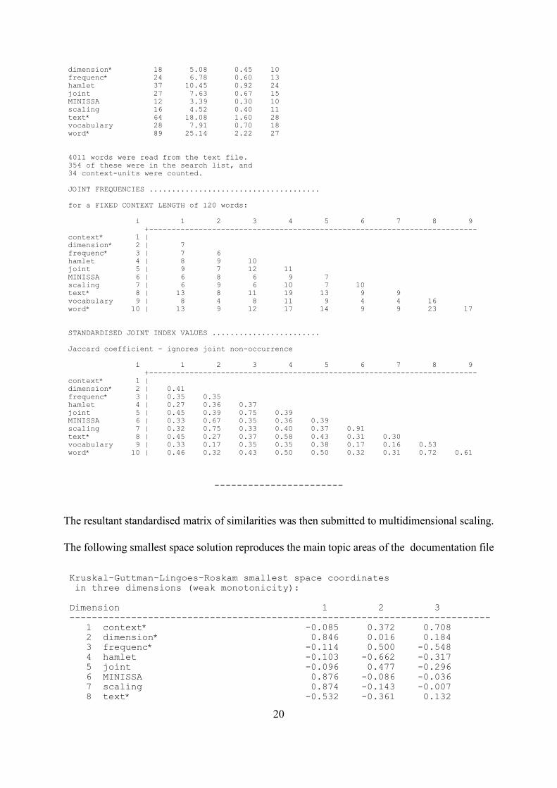
dimension* 18 5.08 0.45 10 frequenc* 24 6.78 0.60 13 hamlet 37 10.45 0.92 24 joint 27 7.63 0.67 15 MINISSA 12 3.39 0.30 10 scaling 16 4.52 0.40 11 text* 64 18.08 1.60 28 vocabulary 28 7.91 0.70 18 word* 89 25.14 2.22 27

4011 words were read from the text file. 354 of these were in the search list, and 34 context-units were counted.

JOINT FREQUENCIES ......................................

for a FIXED CONTEXT LENGTH of 120 words:

i 1 2 3 4 5 6 7 8 9+-------------------------------------------------------------------------

context* 1 | dimension* 2 | 7 frequenc* 3 | 7 6 hamlet 4 | 8 9 10 joint 5 | 9 7 12 11 MINISSA 6 | 6 8 6 9 7 scaling 7 | 6 9 6 10 7 10 text* 8 | 13 8 11 19 13 9 9 vocabulary 9 | 8 4 8 11 9 4 4 16 word* 10 | 13 9 12 17 14 9 9 23 17

STANDARDISED JOINT INDEX VALUES ........................

Jaccard coefficient - ignores joint non-occurrence

i 1 2 3 4 5 6 7 8 9+-------------------------------------------------------------------------

context* 1 | dimension* 2 | 0.41 frequenc* 3 | 0.35 0.35 hamlet 4 | 0.27 0.36 0.37 joint 5 | 0.45 0.39 0.75 0.39 MINISSA 6 | 0.33 0.67 0.35 0.36 0.39 scaling 7 | 0.32 0.75 0.33 0.40 0.37 0.91 text* 8 | 0.45 0.27 0.37 0.58 0.43 0.31 0.30 vocabulary 9 | 0.33 0.17 0.35 0.35 0.38 0.17 0.16 0.53 word* 10 | 0.46 0.32 0.43 0.50 0.50 0.32 0.31 0.72 0.61

-----------------------

The resultant standardised matrix of similarities was then submitted to multidimensional scaling.

The following smallest space solution reproduces the main topic areas of the documentation file

Kruskal-Guttman-Lingoes-Roskam smallest space coordinates in three dimensions (weak monotonicity):

Dimension 1 2 3 --------------------------------------------------------------------------- 1 context* -0.085 0.372 0.708 2 dimension* 0.846 0.016 0.184 3 frequenc* -0.114 0.500 -0.548 4 hamlet -0.103 -0.662 -0.317 5 joint -0.096 0.477 -0.296 6 MINISSA 0.876 -0.086 -0.036 7 scaling 0.874 -0.143 -0.007 8 text* -0.532 -0.361 0.132

21

9 vocabulary -1.124 0.001 0.022 10 word* -0.541 -0.114 0.159 ---------------------------------------------------------------------------

Kruskal's Stress = 0.00279 after 9 iteration(s).

Stress based on approximation to random data = 0.122474

---------------------------------

A pseudo-3-dimensional graphic display of these results appears automatically, as follows.Note that, for easier viewing, these configurations are always rescaled according to their largestabsolute co-ordinate value.

The plotted graphic may be rotated, dragged within the display window, and zoomed to be ableto concentrate on particular areas. Clicking on an individual point will highlight its attachedlabel, which is one of the main vocabulary list items. This is of help in distinguishing pointswhere their labels overlap.

The display can be can be annotated using the graphic editing buttons shown. It can beseparately saved as a graphic image for inclusion in other documents.

Interpretation of MDS solutions may be assisted by reference to hierarchical clustering, as

22

illustrated above. Smallest space analysis, on the other hand, is generally claimed to produce moreeasily interpreted geometric solutions in fewer dimensions than metric procedures like factoranalysis, as well as being more versatile in detecting ordered structures in the data. For furtherdiscussion of the procedures used here, see the references at the end of these notes.

Before settling for any interpretation, however, it is always advisable to check that the MDSsolution in question is reliable, in the sense that it represents a good fit to the information containedin the original matrix and is not a so-called ‘degenerate solution’, dependent upon a single extremevalue. It is also advisable to check that the solution remains reasonably stable under appropriatevariations of the context unit parameters employed to calculate the matrix of joint frequencies onwhich it is based, and if not, to give careful consideration to the possible reasons for this. InHAMLET II, MINISSA offers the conventional MDS diagnostics, accessed from the Data menuin the above graphic display, to try to ensure that solutions accepted for further analysis, forexample, for comparison using INDSCAL or PINDIS, meet the conditions recommended in theauthoritative literature of multidimensional scaling.

These powerful multi-dimensional scaling procedures are described in greater detail in thefollowing sections.

3. Multidimensional Scaling

3.1 MINISSA (Michigan-Nijmegen Smallest Space Analysis) takes as its input a file containinga matrix of standardised joint frequencies, as generated by HAMLET. It is possible to repeatscaling for different combinations of items included in the original word list used by HAMLETto generate the matrix.

The resulting three-dimensional configuration will automatically be displayed in graphic form. thefirst two reference axes appear as a horizontal plane on which labelled points are projectedcorresponding to words or categories in the text file originally subject to analysis. Theconfiguration can be rotated and zoomed for closer examination, printed or saved for inclusion inother documents.

It is possible to examine or edit the file containing the configuration data on which the display isbased using the Data in the graphic display as shown above. Clicking on View/Edit data opensit in a local file editor for this purpose.

Also on the Data menu, there are two additional diagnostic aids in determining the effectivenessof the particular scaling result. The first shows the contributions of the individual points plottedto the final ‘stress’ value reported. This by convention is the measure of the ‘badness of fit’between the distances between the points in the scaled plot and their original distances representedin the similarity values of the initial matrix. The bar chart of these contributions will reveal anypoints which it has been particularly difficult to fit using the MINISSA algorithm into the plot ofreduced dimensionality displayed. The second diagnostic aid is the Shepard diagram, relating theobserved and predicted inter-point distances. A successful scaling is here represented by an evennon-linear or linear relationship with little ‘scatter’ evident.

3.1.1 Using MINISSA

23

•••• At File name: enter the name of the matrix file to be read, or click on the Files menu andselect Open file to search for it. The Files menu also allows you to Reopen files used recentlyto save having to look for them. Alternatively, use the corresponding speed button or Alt/keycombination. The matrix file should have been saved from an earlier run of HAMLET jointfrequencies. When calling MINISSA from within HAMLET joint frequencies, a currenttemporary file containing the scaling results is used automatically.

•••• When a valid file name is found, or if the scaling option is selected within HAMLET jointfrequencies, the vocabulary items available are listed as follows:

•••• It is possible to repeat scaling excluding any of the items included in the current vocabularylist, without repeating the HAMLET joint frequencies analysis each time. From the listdisplayed, simply delete any vocabulary items to be excluded from the scaling process.

24

•••• You may choose to scale these items in one to three dimensions. Click on Scale these itemsto start the scaling process, or Cancel to return to the main MINISSA window.

•••• Once the process has started, as shown by the progress indicator, click on the Abort buttonto abandon scaling at any time.

•••• The resulting configuration is automatically displayed in graphic form. Note that, for ease ofviewing, configurations are always rescaled according to their largest co-ordinate value:

•••• Click on the Data menu item to view or edit the MINISSA output data currently beingdisplayed in detail. For matrices of between 10 and 60 words, this also includes Spence’sapproximation for Kruskal’s Stress based on random data with the same configuration (Spence,1979). The same menu offers, as diagnostic aids, a bar-chart showing the contributions of theindividual points to the final stress value, the Shepard diagram corresponding to the resultsshown , and displays any items which may have been treated as latent categories in theanalysis.

• Use the control buttons shown to rotate and zoom the configuration displayed. Use the keysindicated to rotate and zoom in and out on the display. Click on the axis end points to seethe effect of incremental clockwise rotations of the configuration, where appropriate,

25

with respect to the selected axis. (The numerical keys 1, 2, and 3 have the same result.)Use Configuration to keep track of this process, and save rotated configurations ifrequired.

• Clicking on an individual point will highlight its label,

• Click on menu item Labels to adjust the maximum number of characters of the wordsdisplayed as point labels. Click on a point in the display to highlight its label.

• Click on Grid to toggle the internal lines on the horizontal plane on and off as preferred.

•••• With a mouse button depressed, drag the pointer to a new location and release the mousebutton again to move the display around inside the window, to be able to concentrate onparticular parts of it.

•••• Clicking Draw allows you to draw on the display with the mouse, to highlight features of interest. Clicking Line draws straight lines, from a point where a mouse button is depressedto a point where it is lifted. Clicking Ellipse draws an ellipse within a notional rectangleoutlined using the mouse in a similar manner. Clicking Text causes a box to appear to entertext. On closing this box, move the mouse to the position required and press a mouse buttonto add the text to the image displayed. Click on Refresh to clear any lines and annotationsadded and return to the original image selected. The image as amended must be savedimmediately on completion, as the additions will be lost when the display is reoriented.

•••• Click on Save Display to save the current display as a graphic image file, for inclusion inother documents. The Editor offers limited facilities to draw upon and annotate image filessaved by HAMLET procedures.

• From the main MINISSA window, click on the Files menu and select Save scalingresults, or use the corresponding speed button, to save the scaling output in a file. Clickon the Files menu and select Exit, or use the Alt+F4 key combination, to exit the program.A prompt will appear if any file contents have not been saved.

3.1.1 A note on the treatment of missing values

If MINISSA detects any items in the search list for which HAMLET joint frequencies hasfound no collocations in the original text, these have to be disregarded in producing the scaling,or what is termed a ‘degenerate solution’ results. However, on completion of the scalingprocess, an opportunity is nevertheless offered in saving the results, to record them as extremeoutliers in an otherwise valid final configuration, for possible later comparison with otherresults of applying the same vocabulary list to other texts.

It is, for example, not improbable, if a complex, structured list of categories has been developedtheoretically for application to a number of text sources, that not all items included in the list willbe found to occur explicitly in every text considered. If, however, the user is satisfied that it isjustifiable to retain ‘absent’ items of this kind, for example, if they can plausibly be regarded asimplicit or ‘latent’, rather than simply missing and disregarded, it is not necessary to restrict an

26

investigation to cases where all items are explicitly present.

3.2 Individual Differences Scaling (INDSCAL)

When a series of texts have been analysed using comparable search lists, it is possible to comparethe resulting co-occurrence matrices using another multidimensional scaling procedure calledINDSCAL.

This provides an internal metric analysis of a set of similarity matrices in terms of a weighteddistance model, such that each "subject" (in this case, each text source) is regarded as having aset of dimensional weights which systematically "distort" the group space defined by theoverall relationships of the search list items. All the text sources are thus to be regarded assharing a discourse of the same basic dimensions, but applying different weights to them, toproduce their observed individual matrices of co-occurrences generated by HAMLET JointFrequencies.

INDSCAL is an expressly dimensional model and produces a unique orientation of the axes ofthe group space, in the sense that any rotation will destroy the optimality of the solution andwill change the values of the subject weights. Moreover, the distances in the Group Space areweighted Euclidean, whereas those in the private spaces are simple Euclidean. Because of this,it is not legitimate to rotate the axes of a Group Space to a more 'meaningful' orientation, as iscommonly done in the basic multidimensional scaling model. As will be seen in the followingsection, Procrustean Individual Differences Scaling applies a series of transformations ofdecreasing stringency to the MINISSA configurations generated from the same matrices, in anattempt to bring them into maximal conformity with each other, or with a hypotheticalreference configuration. This allows comparison in greater detail than is provided byINDSCAL, which may nevertheless be found useful in exploring the overall relationshipsbetween a series of texts.

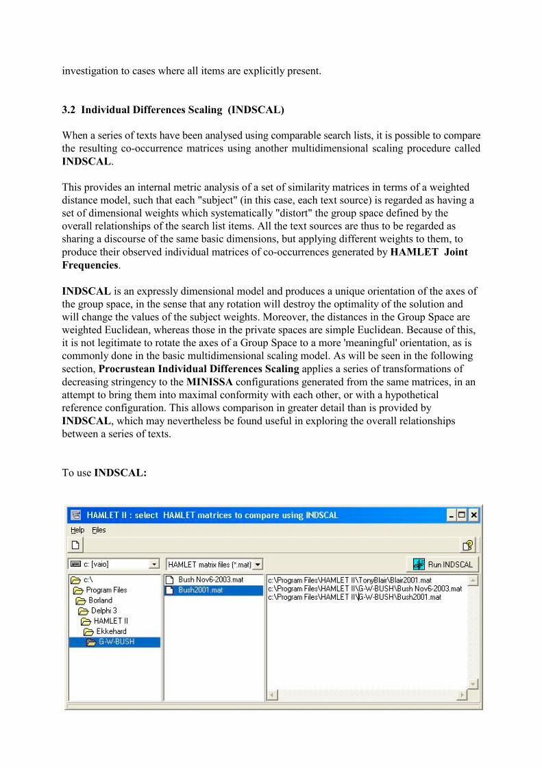
To use INDSCAL:

27

• first select a series of matrices saved from HAMLET Joint Frequencies, by clicking ontheir names in the file list window. This will add the names of the files selected to the right-hand window, after checking that the matrices match those already selected in thevocabulary items they contain. (Note that all windows are resizeable.)

• Then click on the Run INDSCAL button to execute the procedure. The results will bedisplayed in graphic form, in three dimensions, as follows:

• Click on the Next and Previous buttons to switch the display between the Subject Space,showing the text sources, and the Group Space, containing the grouped scaling of thevocabulary items.

• Click on Quit or use the Alt+F4 key combination, to close the display. If an input file hasbeen created, or an output listing exists, these can be saved before closing the program.

3.3 Selecting configurations for detailed comparison using PINDIS

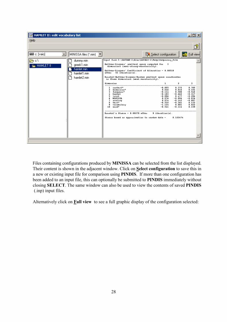
SELECT is used to assemble a series of MINISSA configurations for comparison using PINDIS(Procrustean Individual Differences Scaling ) :

28

•••• Files containing configurations produced by MINISSA can be selected from the list displayed.Their content is shown in the adjacent window. Click on Select configuration to save this ina new or existing input file for comparison using PINDIS. If more than one configuration hasbeen added to an input file, this can optionally be submitted to PINDIS immediately withoutclosing SELECT. The same window can also be used to view the contents of saved PINDIS (.inp) input files.

• Alternatively click on Full view to see a full graphic display of the configuration selected:

29

• Use the keys indicated to rotate and zoom the display.

•••• Click on the Data menu to see the MINISSA output data being displayed in detail and checkthe point contributions to stress and Shepard diagram; Save display to save the graphic.

• Clicking on an individual point will highlight its attached label,

•••• Click on Select configuration to add the configuration displayed to a file to be saved forcomparison using PINDIS.

•••• Close the display and return to the SELECT window to continue.

30

3.4 Procrustean Individual Differences Scaling (PINDIS)

Where equivalent MDS configurations have been produced for a number of different texts, it ispossible to continue the analysis by comparing these results, to produce a picture of therelationships between the various text sources and to examine in detail their similarities anddifferences.

As already described, SELECT, is used to choose a number of configurations generated byMINISSA for analysis by PINDIS, and automatically offers to call PINDIS to compare theconfigurations selected. PINDIS can also be called independently and provided with the namesof suitable input files already created in this way.

The results of a PINDIS analysis are displayed as a series of graphical windows.

By default, the first of these is the centroid configuration, produced by subjecting the original'subject' configurations - for the individual texts selected - to a series of transformations whichpreserve the orderings of the distances between the points corresponding to the words of theoriginal configurations. This represents a kind of median of the individual configurationsconsidered, and acts as a reference point for the examination of the similarities and differencesbetween them. Alternatively, the hypothetical configuration supplied by the user, or, as describedbelow, the configuration adopted by default as the reference for PINDIS comparisons in the eventof employing ‘latent categories’ in the input configurations, in the sense outlined earlier, willappear.

The next plot shown is of the ‘subject space’, which shows the relationship of the originalconfigurations (the “subjects”) which are being compared. The plotted coordinates are theoptimal normalized dimension weights required to bring the individual subjects into conformitywith the reference configuration (i.e. multiplied by the corresponding column sums of squaresof the centroid/hypothesis). Unlike the other displays, which, by convention in MDS, arerescaled for ease of viewing according to their largest co-ordinate value, the original values areplotted here to show the relationship between the texts considered more clearly.

It then remains to examine in turn the individual configurations, as transformed and re-scaled byPINDIS, to determine the extent and source(s) of specific departures from the centroid/initialconfiguration. The individual configurations have been submitted to a succession of decreasinglystringent distortions, the results of which serve to highlight the precise nature of these departures.Although these results may initially appear confusing, they are clearly labelled and will becomeclearer with experience. The simple example given below, comparing only two configurationscontaining a limited number of variables, should help to clarify how to read this necessarilyextensive information.

After estimating the fit achieved by attaching differing weights to the dimensions, and bycombining this with differing dimensional orientations (correlations) – transformations which mayalready be familiar from comparing results derived by factor analysis - the Lingoes/Borg modelgoes on to examine the effects of allowing differing weights and orientations (expressed asdirectional cosines) for the vectors representing the individual words of the vocabulary list in thiscase. Substantial differences at this level will immediately highlight differences in the contextualrelationships of individual words in the texts compared.

31

(The final set of transformations applied allows both dimensional and vector weights to differ,although it is unlikely that this will lend itself to convincing interpretation in application to dataderived from textual analysis.)

3.4.1 Advanced use of PINDIS

•••• Using a hypothesis configuration as a starting pointAs a final stage of analysis, PINDIS also lends itself well to testing goodness of fit of observedconfigurations to a hypothetical or theoretically determined representation, which may be input totake the place of the centroid which is otherwise determined initially. Care is needed that any hypothetical configuration employed has the same format as the various 'subject' configurationswhich are to be compared to it, i.e. co-ordinates must always be entered for the same number ofvocabulary items ('stimuli') as was used in the original MINISSA configurations, and always forall THREE dimensions requested, even if the values for one or even two of these are all to be zero.In this way, the methods described here can be employed strictly in the development of theoreticalmodels of the structures of associations of ideas as they appear in texts of various kinds.

•••• Statistical testsLangeheine (1980) describes tests of significance to permit the evaluation both of singletransformations in PINDIS and of improvements in fit between the various transformations. Histables offer criterion values to test the hypothesis that the fit obtained could be generated bypurely random configurations.

3.4.2 Using PINDIS

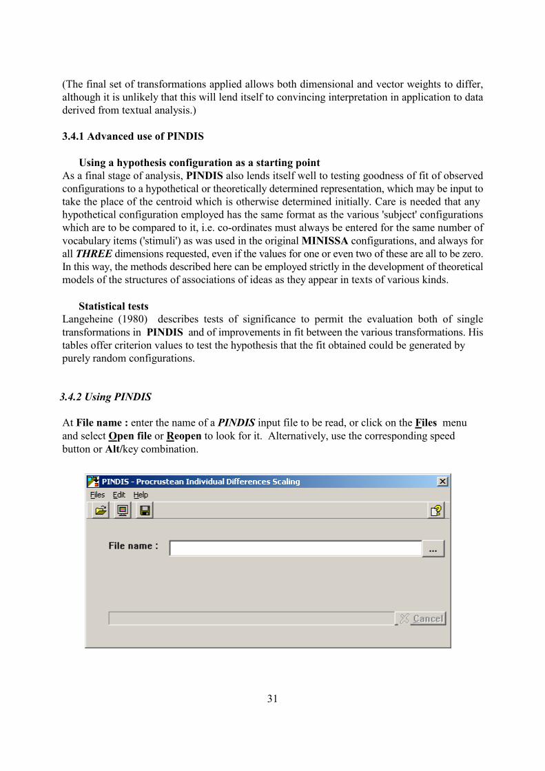
At File name : enter the name of a PINDIS input file to be read, or click on the Files menuand select Open file or Reopen to look for it. Alternatively, use the corresponding speedbutton or Alt/key combination.

32

• When a valid file name is entered, you will be prompted to say if you want to use hypothesisconfiguration as the reference for comparison instead of the centroid, which is the defaultoption here.

•••• If you opt to use a hypothesis configuration you must enter the co-ordinates to be employedin the following window (by default, the values for the first subject configuration are displayedwhen the window is opened):

The results will automatically appear as a series of graphic displays, as described above. Use thebuttons shown to rotate and zoom the configuration displayed. Click on Next and Prev(ious) to

33

cycle through the various configurations of the current PINDIS output, including the individual ( “subject”) configurations as transformed in the analysis. With the exception of the subject space,configurations are rescaled, for ease of viewing, according to their largest absolute co-ordinatevalue.

• Clicking Draw allows you to draw on the display with the mouse , to highlight features ofinterest. Clicking Line draws straight lines, from a point where a mouse button isdepressed to a point where it is lifted. Clicking Ellipse draws an ellipse within a notionalrectangle outlined using the mouse in a similar manner. Clicking Text causes a box toappear to enter text. On closing this box, move the mouse to the position required and pressa mouse button to add the text to the image displayed. Click on Refresh to clear any linesand annotations added and return to the original image selected. The image as amendedmust be saved immediately on completion, as the additions will be lost when the display is

34

reoriented.

• Clicking on an individual point will highlight its label.




•••• Click on View/Edit Data to see the full PINDIS results file.

•••• Click on Save Display to save the current display as a graphic image file, for inclusion inother documents. The Editor also offers limited facilities to draw on and annotate image filessaved by HAMLET procedures

• Close the display to return to the main PINDIS window. Click on the Files menu and selectExit, or use the Alt+F4 key combination, to exit the program. A prompt will appear if anyfile contents have not been saved.

3.5 An example to illustrate the use of PINDIS

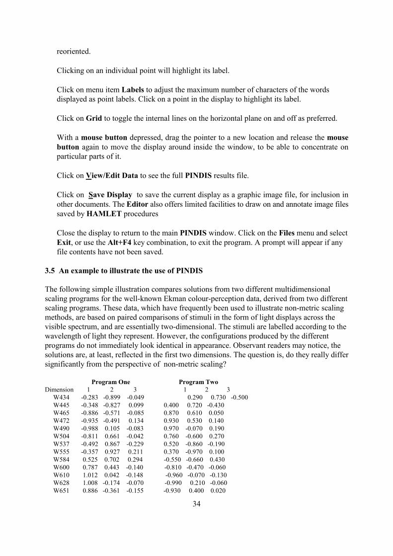
The following simple illustration compares solutions from two different multidimensionalscaling programs for the well-known Ekman colour-perception data, derived from two differentscaling programs. These data, which have frequently been used to illustrate non-metric scaling methods, are based on paired comparisons of stimuli in the form of light displays across thevisible spectrum, and are essentially two-dimensional. The stimuli are labelled according to thewavelength of light they represent. However, the configurations produced by the differentprograms do not immediately look identical in appearance. Observant readers may notice, thesolutions are, at least, reflected in the first two dimensions. The question is, do they really differsignificantly from the perspective of non-metric scaling? Program One Program TwoDimension 1 2 3 1 2 3 W434 -0.283 -0.899 -0.049 0.290 0.730 -0.500 W445 -0.348 -0.827 0.099 0.400 0.720 -0.430 W465 -0.886 -0.571 -0.085 0.870 0.610 0.050 W472 -0.935 -0.491 0.134 0.930 0.530 0.140 W490 -0.988 0.105 -0.083 0.970 -0.070 0.190 W504 -0.811 0.661 -0.042 0.760 -0.600 0.270 W537 -0.492 0.867 -0.229 0.520 -0.860 -0.190 W555 -0.357 0.927 0.211 0.370 -0.970 0.100 W584 0.525 0.702 0.294 -0.550 -0.660 0.430 W600 0.787 0.443 -0.140 -0.810 -0.470 -0.060 W610 1.012 0.042 -0.148 -0.960 -0.070 -0.130 W628 1.008 -0.174 -0.070 -0.990 0.210 -0.060 W651 0.886 -0.361 -0.155 -0.930 0.400 0.020

35

W674 0.881 -0.425 0.262 -0.870 0.500 0.190

For these data, the centroid looks like this:

Clicking on Next displays the subject space as follows, showing that the two solutions arepractically identical, with minor differences only in the third dimension, which can consequentlybe eliminated:

36

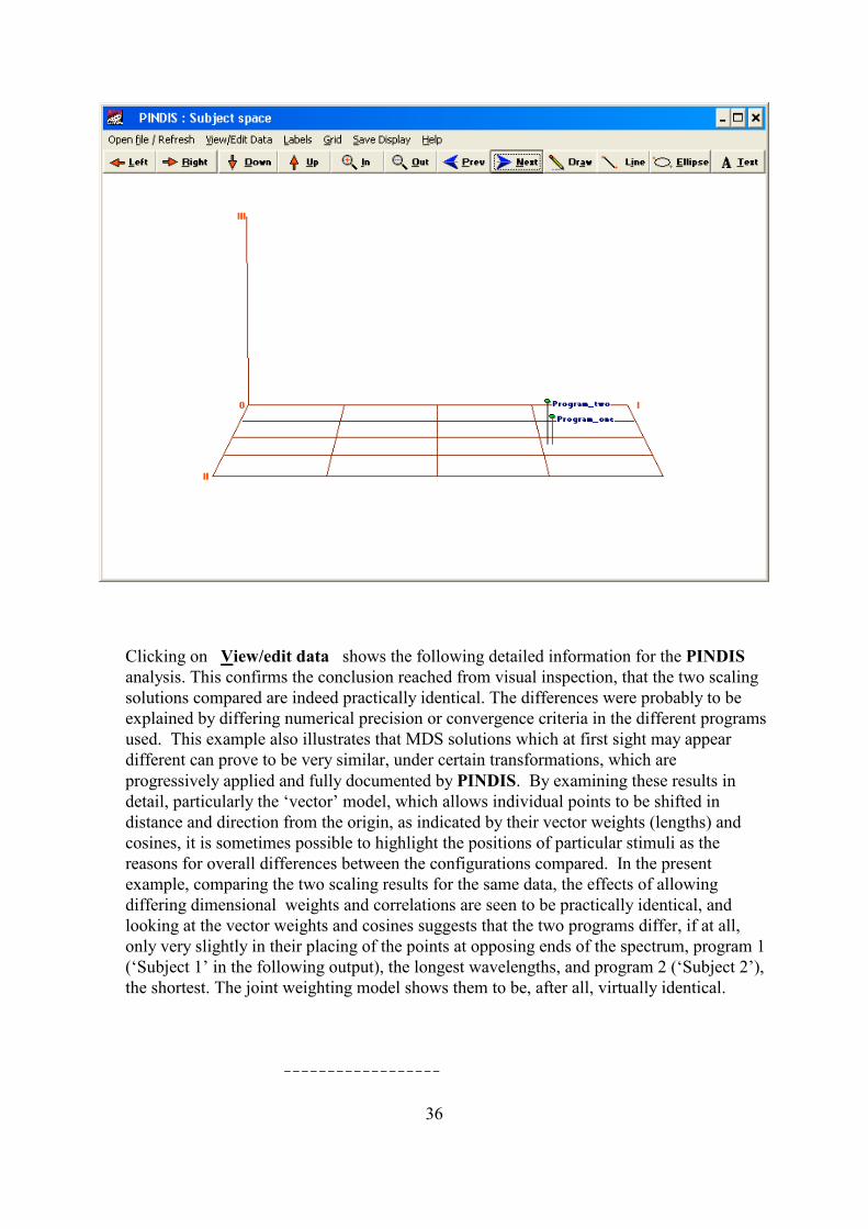
•••• Clicking on View/edit data shows the following detailed information for the PINDISanalysis. This confirms the conclusion reached from visual inspection, that the two scalingsolutions compared are indeed practically identical. The differences were probably to beexplained by differing numerical precision or convergence criteria in the different programsused. This example also illustrates that MDS solutions which at first sight may appeardifferent can prove to be very similar, under certain transformations, which areprogressively applied and fully documented by PINDIS. By examining these results indetail, particularly the ‘vector’ model, which allows individual points to be shifted indistance and direction from the origin, as indicated by their vector weights (lengths) andcosines, it is sometimes possible to highlight the positions of particular stimuli as thereasons for overall differences between the configurations compared. In the presentexample, comparing the two scaling results for the same data, the effects of allowingdiffering dimensional weights and correlations are seen to be practically identical, andlooking at the vector weights and cosines suggests that the two programs differ, if at all,only very slightly in their placing of the points at opposing ends of the spectrum, program 1(‘Subject 1’ in the following output), the longest wavelengths, and program 2 (‘Subject 2’),the shortest. The joint weighting model shows them to be, after all, virtually identical.

------------------

37

An example comparing two scalings of the EKMAN colour similiarity data

Fit of Centroid Configuration 0.011047 0.011047

Centroid configuration 1 W434 -0.1103 -0.2149 -0.0606 2 W445 -0.1336 -0.1980 -0.0337 3 W465 -0.2596 -0.1139 -0.0091 4 W472 -0.2732 -0.0877 0.0290 5 W490 -0.2553 0.0726 -0.0097 6 W504 -0.1794 0.2087 -0.0026 7 W537 -0.0893 0.2443 -0.0886 8 W555 -0.0542 0.2685 0.0090 9 W584 0.1684 0.1666 0.0913 10 W600 0.2348 0.0818 -0.0210 11 W610 0.2660 -0.0339 -0.0172 12 W628 0.2564 -0.0975 0.0098 13 W651 0.2237 -0.1408 0.0117 14 W674 0.2057 -0.1557 0.0919

**** Perspective Origins ****

Subject 1 -0.1606 -0.2959 1.3429 2 0.0935 0.3574 -1.1140

**** Analytic Solutions for Individual Configurations ****

**** Configuration for Subject 1 **** **** Program one

1) Similarity Transformations

Normed scalar for unconditional weights: 1.000000

1 W434 -0.1153 -0.2246 -0.0203 2 W445 -0.1322 -0.2022 0.0181 3 W465 -0.2582 -0.1100 -0.0423 4 W472 -0.2720 -0.0860 0.0154 5 W490 -0.2537 0.0735 -0.0430 6 W504 -0.1821 0.2123 -0.0276 7 W537 -0.0845 0.2515 -0.0706 8 W555 -0.0554 0.2622 0.0501 9 W584 0.1648 0.1619 0.0907 10 W600 0.2310 0.0802 -0.0202 11 W610 0.2718 -0.0362 -0.0180 12 W628 0.2590 -0.0930 0.0025 13 W651 0.2200 -0.1369 -0.0231 14 W674 0.2069 -0.1526 0.0883

Fit of subject to centroid/hypothesis --- S(Z,X) = 0.988953

2) Dimensional-weighting Transformations

Dimensional Weights: 1.0003 1.0025 0.7870 Dimensional Correlations:

38

0.9999 0.9996 0.8223

Fit --- S(ZW,X)= 0.990200

3) Perspective Models - Vector Weighting

Translation of Individual Configuration: -0.0386 0.0313 0.1126 Stimuli: Vector Weights: Vector Cosines: 1 W434 1.0907 0.9916 2 W445 1.0845 0.9863 3 W465 0.9743 0.9946 4 W472 0.9928 0.9992 5 W490 0.9807 0.9951 6 W504 1.0011 0.9973 7 W537 1.0313 0.9983 8 W555 1.0336 0.9931 9 W584 0.9738 0.9999 10 W600 0.9644 0.9999 11 W610 0.9928 0.9997 12 W628 0.9648 0.9992 13 W651 0.8868 0.9915 14 W674 0.9694 0.9999

Fit --- S(VZ,X)= 0.992072

4) Joint Weighting Solution

Dimensional Weights: 1.0055 1.0075 0.8054 Vector Weights: 1 W434 1.0138 2 W445 0.9836 3 W465 0.9874 4 W472 0.9866 5 W490 0.9938 6 W504 1.0105 7 W537 1.0107 8 W555 0.9748 9 W584 0.9922 10 W600 0.9790 11 W610 1.0176 12 W628 0.9968 13 W651 0.9698 14 W674 1.0057

Fit --- S(VZW,X)= 0.990303

**** Configuration for Subject 2 **** **** Program two

1) Similarity Transformations

Normed scalar for unconditional weights: 1.004231

1 W434 -0.1041 -0.2028 -0.1004 2 W445 -0.1335 -0.1916 -0.0851 3 W465 -0.2582 -0.1165 0.0241 4 W472 -0.2714 -0.0884 0.0422 5 W490 -0.2540 0.0709 0.0237 6 W504 -0.1747 0.2028 0.0224 7 W537 -0.0931 0.2344 -0.1057 8 W555 -0.0524 0.2719 -0.0321 9 W584 0.1701 0.1694 0.0908

39

10 W600 0.2360 0.0824 -0.0217 11 W610 0.2573 -0.0312 -0.0162 12 W628 0.2509 -0.1010 0.0171 13 W651 0.2250 -0.1431 0.0463 14 W674 0.2022 -0.1570 0.0945

Fit of subject to centroid/hypothesis --- S(Z,X) = 0.988953

2) Dimensional-weighting Transformations

Dimensional Weights: 0.9884 0.9864 1.2016 Dimensional Correlations: 0.9999 0.9996 0.9109

Fit --- S(ZW,X)= 0.990200

3) Perspective Models - Vector Weighting

Translation of Individual Configuration: -0.0301 0.0329 0.1144 Stimuli: Vector Weights: Vector Cosines: 1 W434 0.8787 0.9832 2 W445 0.8866 0.9753 3 W465 1.0153 0.9965 4 W472 0.9965 0.9996 5 W490 1.0188 0.9954 6 W504 1.0021 0.9968 7 W537 0.9764 0.9988 8 W555 0.9708 0.9936 9 W584 1.0221 1.0000 10 W600 1.0283 1.0000 11 W610 0.9879 0.9994 12 W628 1.0108 0.9994 13 W651 1.0833 0.9945 14 W674 1.0051 1.0000

Fit --- S(VZ,X)= 0.992053

4) Joint Weighting Solution

Dimensional Weights: 0.9956 0.9902 1.1956 Vector Weights: 1 W434 0.9883 2 W445 1.0172 3 W465 0.9994 4 W472 1.0026 5 W490 0.9923 6 W504 0.9787 7 W537 0.9810 8 W555 1.0145 9 W584 0.9872 10 W600 1.0089 11 W610 0.9697 12 W628 0.9917 13 W651 1.0215 14 W674 0.9771

Fit --- S(VZW,X)= 0.990256

Normalized Dimension Weights

40

Subject Communality 1 2 3 1 0.9902 0.7701 0.6146 0.1397 2 0.9902 0.7609 0.6047 0.2134 Mean Communality 0.9902 0.5860 0.3717 0.0325

--- Table of Subject Communalities for PINDIS Transformations ---

Transformation Z,X[i] ZW[i],X[i] Z[i]W[i],X[i] V[i]Z,X[i] V[i]Z[i],X[i] V[i]ZW[i],X[i] ------------------------------------------------------------------------------

1 0.99 0.99 0.99 0.99 1.00 0.99 2 0.99 0.99 0.99 0.99 1.00 0.99

Mean 0.99 0.99 0.99 0.99 1.00 0.99

------------------------------------------------------------------------------ * 0.0 means that particular PINDIS transformation was not used.

For further information about these procedures, see the references below, especially Davies andCoxon (1982) and Borg and Groenen (2005).

4. Correspondence Analysis (CA)

represents the row and column categories of the input matrix as points in the same dimensionality.It is closely related to other procedures which seek to represent row and column variables in thesame space, using a singular value decomposition. It is important to realise that CA considers onlyinteractive factors by explicitly neglecting the magnitude effect after decomposition. Because thecanonical ("optimal") scores reported are row and column conditional, it is advisable to avoid inter-set point distance interpretation, however tempting this may be, when using correspondenceanalysis.The input matrix is first normalized by dividing each row entry by the square root of theproduct of the corresponding row and column totals, their geometric mean. This removesdifferences in the marginal totals and expresses each cell as a proportion.

The second step finds the basic structure of the resultant matrix A by singular valuedecomposition, producing summary row and column vectors ( U and V) and a diagonal matrixof singular values d corresponding to the columns of A, so that A = Ud(VT). The matrices Uand V are in fact the eigenvectors of the matrices of row and column cross-products of A, andthe d values are related to their (identical) eigenvalues (d=sqrt(D*(n-1)), where D is thediagonal of eigenvalues and n is the number of rows in A). The first singular value in d isalways 1.0. It corresponds to the independence model of chi-squared expected values, and isignored in subsequent analysis.

It is important to check that the eigenvalues remaining after ignoring the first one are in factlarge enough to justify continuing with the analysis. Reference should be made to the chi-

41

squared contributions of each dimension of "inertia" and to the overall chi-squared value for theanalysis.

The method implemented here is equivalent to HOMALS in SPSS, which uses an alternatingleast squares algorithm which is considered more suitable for large numbers of cases.

For further information on this procedure see Weller and Romney (1990), Greenacre (1993).

4.1 Using Correspondence Analysis

At File name : enter the name of the file of context unit profiles to be read, or click on the Filesmenu and select Open file, or use the appropriate speed button, to search for it. From the Filesmenu, it is also possible to Reopen directly files used recently.

When a valid file name is entered, the categories included are displayed. Select the number ofdimensions to be reported (2 or 3), and click Include these categories to start the analysis.

Click Cancel to return to the main HAMLET window. Once the process has started, click onCancel to abandon the analysis at any time.

The resulting configuration is automatically displayed in graphic form.

Close this display to return to the Correspondence Analysis window shown above.

42

•••• Click on the Data menu item to view or edit the correspondence analysis result currently beingdisplayed in detail.

• Use the control buttons shown to rotate and zoom the configuration displayed. Use the keysindicated to rotate and zoom in and out on the display.




•••• Clicking Draw allows you to draw on the display with the mouse, to highlight features of interest. Clicking Line draws straight lines, from a point where a mouse button is depressedto a point where it is lifted. Clicking Ellipse draws an ellipse within a notional rectangleoutlined using the mouse in a similar manner. Clicking Text causes a box to appear to enter

43

text. On closing this box, move the mouse to the position required and press a mouse buttonto add the text to the image displayed. Click on Refresh to clear any lines and annotationsadded and return to the original image selected. The image as amended must be savedimmediately on completion, as the additions will be lost when the display is reoriented.

•••• Click on Save Display to save the current display as a graphic image file, for inclusion inother documents. The Editor also offers limited facilities to draw upon and annotate imagefiles saved by HAMLET procedures.

• Close the display to return to the Correspondence Analysis window. Click on the Filesmenu and select Exit, or use the Alt+F4 key combination, to exit the program. A promptwill appear if any file contents have not been saved.

5. Basic utilities for looking at word usageHAMLET for Windows offers the following additional utilities, to assist in exploration of wordusage in texts intended for further analysis, and assist in the creation of search lists for use with themain procedure, HAMLET joint frequencies.

5.1 WORDLIST displays a sorted list of words found in a file of text. Any character-stringcontaining letters and numerals may be considered as a ‘word’ for this purpose. WORDLIST canalso be used to check how HAMLET will read the contents of a file and help to avoid errors inlater analysis. Files created with WORDLIST can be compared with other lists in the same formatusing the companion procedure COMPARE.

5.1.1 Using WORDLIST

•••• At File name : enter the name of the file to be read, or click on the Files menu and selectOpen file to search for it. The Files menu also allows you to Reopen directly files usedrecently to save having to look for them. Alternatively, use the corresponding speed button orAlt/key combination. If the text is in a language other than English, use the pull-down menuon the right of the control panel to select the appropriate lexicographic conventions to beemployed.

44

•••• To limit counting to words according to length, enter the minimum and maximum numberof letters in the boxes indicated.

•••• To limit counting by initial letters, enter the relevant letters in the box provided, otherwiseleave the default entry "list all words occurring ..".

•••• Toggle the appropriate button to list words in forward alphabetical order or descending orderof frequency.

•••• Click on Create a Word List to start counting words.

The resulting list will be displayed in a temporary edit window when finished. The progressindicator shows text reading in process. Click on the Cancel button to stop the counting processat any time.

•••• Click on the Files menu and select Save word list, or use the corresponding speed button, tosave the resulting list in a file.

5.2 COMPARE is used to compare pairs of the sorted vocabulary lists produced by thecompanion program WORDLIST. It simply displays in parallel columns the frequencies for anywords which appear in both lists. The results can then be saved to compare with other listsproduced by WORDLIST or by earlier applications of COMPARE itself.

Percentage frequencies are shown, based on the words counted by WORDLIST in the originaltext, or are the weighted averages of the percentages for the same words in pairs of files whosefrequencies have been combined by COMPARE.

45

5.2.1 Using COMPARE

•••• At Wordlist File One: and Wordlist File Two: enter the names of the files to be compared,or click on the Files menu and select Open file to search for them. Alternatively, use thecorresponding speed button or Alt/key combination. If the lists to be read are in a languageother than English, use the pull-down menu on the right of the control panel to select theappropriate lexicographic conventions.

•••• Click on Create list of words common to both files to start comparison. The results willbe displayed in a temporary edit window when complete. Click on Cancel to stop the processat any time. Patience may be needed when comparing large lists, depending on the computingresources you have available. If progress appears very slow, check for continuing disk activitybefore concluding that there is an error.

•••• Click on the Files menu and select Save word list to save the resulting list in a file.

5.3 KWIC (Key_Word_In_Context) can be used to produce traditional single line KWIClistings, with one or more keywords in the centre, or display the keyword(s) within a larger blockof text.

5.3.1 Using KWIC

• At File name: enter the name of the file to read, or click on the Files menu and select Openfile to search for it. The Files menu also allows you to Reopen directly files used recently tosave having to look for them. Alternatively, use the corresponding speed button or Alt/keycombination. If the text to be read is in a language other than English, use the pull-down menu

46

on the right of the control panel to select the appropriate lexicographic conventions to apply.

• At Search for : enter a word or phrase to search for - this may include the ‘wild card’characters ‘@’ and ‘*’, causing individual letters corresponding to the position of thecharacter ‘@’, and all characters after, and including, the position of the character ‘*’, tobe ignored in searching. This, for example, provides a way to treat as equivalent words which differ only in their suffixes, e.g. plural forms. Click on the adjacent button to see adisplay of all of the words in the file selected, with their frequencies. You can select andcopy words from this window into the main panel using the mouse. With the left mousebutton :clicking on 'Words >' reverses the order of the items listed, and clicking on 'Freq.'causes the columns to swap positions. Clicking anywhere in the vocabulary list with theright mouse button switches the listing between alphabetical and frequency order.

•••• You can select and copy words from this list into the main panel. Checking the appropriateitem below will cause occurrences of the words entered to be listed as a phrase, or separately.

•••• Enter the size of the context to display the keyword, if found, in lines of text: (1 ≤≤≤≤ n ≤≤≤≤ 15).

•••• Click on Create Key_Word_In_Context List to start searching the text for the string to beidentified. The results will be displayed in a temporary edit window when completed. Clickon Abort to stop the process at any time.

•••• Click on the Files menu and select Save KWIC list, or use the corresponding speed button,to save the resulting list in a file.

.

5.4 Text Profiledisplays a profile of the distributions of word and sentence lengths for a given text file. This showsmean word and sentence lengths, with dispersion statistics and a histogram for each distribution.It therefore supplements the information available from Wordlist, for the entire text file, without

47

the restrictions which may be applied in that procedure.

•••• At File name: , enter the name of the file to be read, or click on the Files menu and selectOpen file to search for it, or use the corresponding speed button with the same effect. TheFiles menu also allows you to Reopen directly files used recently to save having to look forthem.

•••• Select the Internet item from the Files menu, or the corresponding speed button, to access afile from the Internet.

•••• Use the pull-down menu at the top right of the display to select the correct character set to useif the text contains words of a language other than English.

•••• If necessary, amend the set of characters marking the end of sentences in this text.

•••• Click on Create text profile to start the process. The progress indicator shows the text beingread. Click on Cancel at any time to interrupt the process. The text profile is displayed asfollows:

48

•••• The graphic image may be saved by clicking on the Save button at the bottom of the display.Click Close to return to the previous window.

•••• On clicking Save results on the main menu, or on closing the procedure, you will be promptedto save a file containing the equivalent results in text form.

49

I. References and further reading

I.Borg and P.Groenen, Modern Multidimensional Scaling:Theory and Applications, 3rd,Edition, Springer, (2005).

A.P.Brier "HAMLET: A Pascal Program to Count Joint Frequencies of Words in a Text",Siegener Periodicum für internationale empirische Sozialwissenschaft, 4,1,(1985),pp.177-196

A.P.Brier and A.Reiter "Methode zur Ermittlung von Ähnlichkeitswerten von Kontextwörternund ihre Anwendung in einer ideologiekritischen Zeitschriftsanalyse" in Manfred Thaller, AlbertMüller (Hg.), Computer in den Geisteswissenschaften: Konzepte und Berichte, Studien zurHistorischen Sozialwissenschaft Band 7, Frankfurt/Main, Campus, (1989)

A.P.Brier "Natural Language Processing and the Analysis of Structure", European Political DataNewsletter, 68, September 1988, pp.39-53

A.P.Brier and F.-M. Bahr "Computer-Assisted Text Analysis in a Teaching Environment", AnnualJoint Sessions of the European Consortium for Political Research, Bochum, April 1990, reprintedin SocInfo, CTI Centre for Sociology and the Policy Sciences, Newsletter Four, May 1991.

A.P. Brier and B. Hopp "HAMLET a Multidimensional Scaling approach to text-orientedpolicy analysis", Journal of Diplomatic Language 2,1, (2005) (http://www.jdonline.org/IIbrier.html)

M.J.Brusco "An enhanced branch-and-bound algorithm for a partitioning problem," BritishJournal of Mathematical and Statistical Psychology, 56, (2003) pp. 83-92.

M.J.Brusco, and M.Stahl,M. Branch-and-Bound Applications in Combinatorial DataAnalysis, New York, Springer (2005).

J.D.Carroll J.D. and J.J.Chang “Analysis of individual differences in multidimensional scalingvia n-way generalization of ‘Eckhart-Young’ decomposition” in: Psychometrika, 35, (1970)pp.283-319.

T. F. Cox and M. A. A. Cox, Multidimensional Scaling, Chapman and Hall, 2nd edition (2004).

A.P.M.Coxon The User’s Guide to Multidimensional Scaling, Heinemann (1982).

P.M.Davies and A.P.M.Coxon (eds.) Key Texts in Multi-dimensional Scaling, (1982).

B.S.Everitt and S.Rabe-Hesketh, The Analysis of Proximity Data, Arnold, (1996)

M.G.Greenacre, Correspondence Analysis in Practice, Academic Press (1993).

H.P.Iker "An historical note on the use of word-frequency contiguities in content analysis",

50

Computers and the Humanities, 8, (1974).

S.C Johnson, “Hierarchical clustering schemes”, Psychometrika, 32, (1967), pp.241-254.

K.Krippendorf Content Analysis : An Introduction to its Methodology, Newbury Park, CA.& London, Sage Publications, 2nd Edition.(2004)

J.B.Kruskal "Multidimensional scaling by optimizing goodness of fit to a non-metric hypothesis,"Psychometrika, 29, (1964), pp.1-27.

R.Langeheine Approximate Norms and Significance Tests for the LINGOES-BORGProcrustean Individual Differences Scaling (PINDIS), Institut für die Pädagogik derNaturwissenschaften, University of Kiel (1980).

J.C.Lingoes and I.Borg "A direct approach to individual differences scaling using increasinglycomplex transformations," Psychometrika, 44, (1979), pp.491-519.

R.R.Sokal and P.H.Sneath, Principles of Numerical Taxonomy, Freeman, (1963)

I.Spence, “A simple approximation for random rankings stress data”, Multivariate BehavioralResearch, 14, (1979), pp.355-365, reproduced in Davies and Coxon,(1982).

S.C.Weller, A.K.Romney, Metric Scaling – Correspondence Analysis, SAGE, QuantitativeApplications in the Social Sciences, 75, (1990).

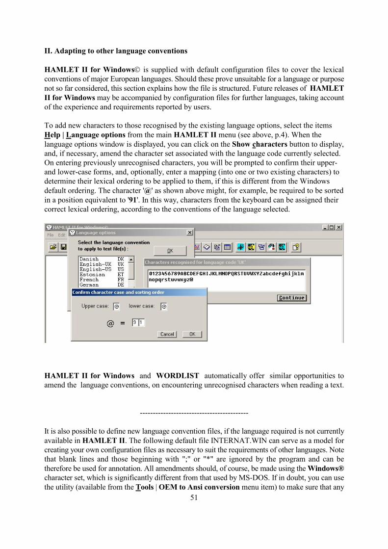
51

II. Adapting to other language conventions

HAMLET II for Windows is supplied with default configuration files to cover the lexicalconventions of major European languages. Should these prove unsuitable for a language or purposenot so far considered, this section explains how the file is structured. Future releases of HAMLETII for Windows may be accompanied by configuration files for further languages, taking accountof the experience and requirements reported by users.

To add new characters to those recognised by the existing language options, select the itemsHelp | Language options from the main HAMLET II menu (see above, p.4). When thelanguage options window is displayed, you can click on the Show characters button to display,and, if necessary, amend the character set associated with the language code currently selected.On entering previously unrecognised characters, you will be prompted to confirm their upper-and lower-case forms, and, optionally, enter a mapping (into one or two existing characters) todetermine their lexical ordering to be applied to them, if this is different from the Windowsdefault ordering. The character '@' as shown above might, for example, be required to be sortedin a position equivalent to '91'. In this way, characters from the keyboard can be assigned theircorrect lexical ordering, according to the conventions of the language selected.

HAMLET II for Windows and WORDLIST automatically offer similar opportunities toamend the language conventions, on encountering unrecognised characters when reading a text.

------------------------------------------

It is also possible to define new language convention files, if the language required is not currentlyavailable in HAMLET II. The following default file INTERNAT.WIN can serve as a model forcreating your own configuration files as necessary to suit the requirements of other languages. Notethat blank lines and those beginning with ";" or "*" are ignored by the program and can betherefore be used for annotation. All amendments should, of course, be made using the Windows®character set, which is significantly different from that used by MS-DOS. If in doubt, you can usethe utility (available from the Tools | OEM to Ansi conversion menu item) to make sure that any

52

text files to be read are compatible with Windows.

; INTERNAT.WIN - Sample Windows collating sequence;; * NB In reading the following file, blank lines and comments; * (running from ";" or "*" to EOLN) are ignored *;; This file may be edited to include any other characters which may; be required. Only the characters specified here will be used in; word searching routines in the HAMLET package for Windows.; Currently, two sections are defined, as detailed below:; Section headings may be enclosed by any pair of bracket characters.;; [UPCASE]; This section contains all information needed for to convert characters; in language set to upper-case equivalents. It also creates a set of; characters which are used in other routines. Entries must consist of; pairs of characters,the upper-case form followed by the lower-case; equivalent. Numerals if they are to be recognised should also be; included here, as repeated pairs, as should any other valid characters; for which there is no normal upper-case equivalent in the printed; language.;; [MAPPING]; The mapping section contains all character mappings significant for; the correct lexical ordering of lists of words in a given language.; Only special or accented characters need to be specified, since any; characters not specified will collate in the normal ASCII order.; The order of entries in this section is irrelevant.

[UPCASE]00112233445566778899AaÄäÅåÁáÀàÂâBbCcÇçDdEeËëÉéÈèÊêFfGgHhIiÏïÍíÌìÎîJjKkLlMmNnÑñOoÖöÓóÒòÔôPpQqRrSsßßTtUuÜüÚúÙùÛûVvWwXxYyYÿZz

*************************** END OF UPCASE SECTION ***************************

[MAPPING]******************************************************** Mappings for correct ordering of European languages *

* GermanicÄ=AEÖ=OEÜ=UEä=aeë=oeü=ueß=SS* OtherÉ=EEé=eeè=eeê=eeÇ=Cç=cá=aaà=aaâ=aaû=uuô=oo

53

î=iiï=iiÑ=NNñ=nnù=uu

;**************************;* Other example mappings *;Å=A;å=a;Æ=AE;æ=ae;¢=C;ë=e;í=ii;ì=ii;ó=oo;ò=oo;ú=uu;ù=uu;ÿ=ye;¥=Y

*************************** END OF MAPPING SECTION ***************************

************************ END OF INTERNAT.WIN ************************

-------------------------------------------

Having created a similar configuration file for a language not currently covered by HAMLET IIfor Windows, for example, a file containing Polish language conventions, called POLISH.CFG,you should first copy this to the directory in which the main HAMLET routines are installed(normally this will be called C:\Program files\HAMLET II\ ).

Next, load the main HAMLET II program, select Help | Language options from the main menu,and click the Edit button to enter the following window:

54

Simply enter the relevant 2-character Windows language code together with the name of the newly-created file containing the corresponding lexicographic conventions, and click on OK to add thiscode to those already available. You can check the effect of a new file by again clicking on theShow characters button, as described above.

III. Technical details

HAMLET II for Windows requires at least 10 Megabytes of space to install on a hard disk orsimilar medium. All the necessary files are automatically installed in one main directory, asdirected at the time of installation. All temporary files are stored in the directory to whichpermission is assigned in the current Windows setup for this purpose.

Language convention files with the extensions .win (or .cfg ), as described above (pp.36-39),must be placed together with the file HAMLET.INI in the main installed directory.

Files with the following default extensions may be saved in the course of working with HAMLET,to store the following program data and results:

.voc - vocabulary lists for use with HAMLET Joint Frequencies

.mat - matrix of co-occurrences of word pairs, from HAMLET Joint Frequencies used as input to MINISSA, Cluster Analysis, or INDSCAL.xpr - context profiles created by HAMLET Joint Frequencies for use with Correspondence Analysis.xpc - results of Correspondence Analysis.ham - output listing from HAMLET Joint Frequencies.txt - listing of word clusters identified by Cluster Analysis.min – MINISSA output listing, accessed by SELECT to generate input to PINDIS.inp – PINDIS input file.pin – PINDIS output listing

55

.bmp, .jpg - Graphic files to store results displayed by MINISSA, PINDIS, Correspondence Analysis, INDSCAL and PROFILE.lst - Word list file, generated by Wordlist or Compare.kwc – Key-Word-In-Context listing

Note that, apart from .bmp and .jpg, these are only conventions, and may be varied to suitthe convenience of individual users should they conflict with file extensions already assignedto other software in use on the machine on which HAMLET is installed.

hamlet – a multidimensional scaling approach to textual ... · be of interest, the non-metric...

Documents