Hamiltionian path based shadow removal

Clement Fredembach and Graham D. FinlaysonSchool of Computing Sciences

University of East AngliaNorwich, NR4 7TJ, UK

{cf,graham}@cmp.uea.ac.uk

Abstract

For some computer vision tasks, the presence of shadows in images cancause problems. For example, object tracks can be lost as an object crossesover a shadow boundary. Recently, it has been shown that it is possible toremove shadows from images. Assuming that the location of the shadowsare known, shadow-free images are obtained in three steps. First, the imageis differentiated. Second, the derivatives at the shadow edge are set to zero.Third, reintegration delivers an image without shadows. While this processcan work well, the resultant shadow free image often has artifacts and, more-over, the reintegration is an expensive computational procedure.

In this paper we propose a method which can produce shadow free imagesquickly and without artifacts. Our algorithm is based on two observations.First, that shadows in images are closed regions and if they are not closed ar-tifacts can result during reintegration. Thus we propose to extend the existingmethods and enforce the constraint that shadow boundaries must be closedprior to reintegration. Second, that the standard reintegration method used(solving a 2D Poisson equation) also, necessarily, introduces artifacts. Thesolution here is to reintegrate shadow and non shadow regions almost sepa-rately. Specifically, we reintegrate the image along a Hamiltonian path thatenters and exits the shadow regions once. Detail that was masked out at theshadow boundary is then infilled in a second step. The resulting reintegratedimage has much fewer artifacts. Moreover, since the reintegration method ispath based it is both simple and fast. Experiments validate our approach.

1 Introduction

A shadow is cast in a scene when an object lies in the path of the direct illuminationsource. If a scene is illuminated by two or more sources, then the shadow and non-shadowregions of an object may differ not just in terms of their relative brightness, but also interms of their relative colour. For example, in a typical outdoor scene, the non-shadowparts of the image are illuminated by a mixture of direct sunlight and light from the sky. Incontrast, shadow regions are lit only by skylight (see Fig. 6 for an illustration) . These twoillumination sources differ significantly both in their brightness and their colour, and, asa result, so do the resulting image pixel values corresponding to shadow and non-shadowregions.

In many computer vision applications such as tracking, scene analysis and objectrecognition it has been shown that shadows hamper algorithm performance [1,2]. Ad-ditionally, one may also wish to remove shadows for cosmetic reasons since they areoften accidental and/or unwanted artifacts in a photograph e.g. in some conditions (flash)it can be impossible to take shadow-free images. Finally, when working with images thathave a large bit depth, the presence of a shadow is indicative of a high dynamic rangeimage that probably cannot be properly displayed. If we can remove the shadow, we areable to compress the dynamic range.

A simple framework for shadow removal has recently been proposed [3]. Given animage containing both shadow and non-shadow regions, and assuming the location ofshadows are known, shadows can be removed by a process of differentiation, masking(the shadow) and reintegration. In detail, the x and y derivatives are taken at each pointin the image. The x and y derivatives at pixels on shadow edges are set to 0. Then theresulting derivative field is reintegrated. In the original work reintegration was performedby formulating the problem as solving a 2D Poisson equation. Using this method, onecan recover a colour image whose content is the same as the original image, but whereshadows have been removed.

While this approach can often give good results, the resulting shadow-free imagescan often have undesirable artifacts. Indeed, one might reasonably expect artifacts. Thereason for this is the non integrability that occurs because setting shadow edge deriva-tives to 0 (a local effect) is translated to global reintegration errors. Reintegrated imagesoften have smearing artifacts and may look flatter than the original image. In addition,reintegration posed as solving the Poisson equation is computationally expensive and, forhigh-resolution images, a time consuming task.

In recent work [4] it was shown that the reintegration problem can be reformulated asa 1-dimensional problem by integrating the image along a 1D path that visits each pixelin the image once and only once. Formally, reintegration is along a Hamiltonian path.However, while this approach addresses the issue of computational complexity, it is alsonon-robust in the sense that the recovered images can still have visible artifacts.

Our aim in this paper is to consider the reintegration problem more carefully andto propose a robust, computationally simple 1-dimensional reintegration procedure. Weachieve this aim by investigating the reasons that artifacts arise in the 2D and 1D rein-tegration schemes which have been proposed to date. We show that robust reintegrationrequires that shadow boundaries should be closed and we propose a method to enforcethis property. In addition, to obtain artifact free images we argue that we must carefullychoose a 1-dimensional path through the image pixels. We argue that for 1-d reintegra-tion artifacts occur as we enter and exit shadows and so provide a method which producesHamiltonian paths that exit and enter each shadow regions only once. Our final contribu-tion is to show that shadow edges themselves do not have to be fully reintegrated but canbe later inpainted in the image. We present results which show that our new reintegrationscheme gives very good shadow-free images which have significantly fewer artifacts thanimages obtained using either a 2D or naive 1D approach.

2 Background

All computations in this paper are carried out in the log domain, so ratios between pixelsare preserved. So, though not explicitly stated, all computed images are exponentiatedwhen making outputs.

Let I denote the log of an image. Its gradient,∇I is

∇I = (∂ I∂x

,∂ I∂y

) (1)

Now, suppose the shadow edges,S, can be found (e.g. using the method set forth in [5]and in section 2.1) and that their derivatives can be thresholded using a functionT(∇I)such that

T(∇I) = 0 if |∇I | ∈ S

= ∇I otherwise

How can I be recovered fromT(∇I)? This is not an easy question to answer since agradient image is composed of two number per pixel but the reintegrated image has asingle number per pixel. Besides, a 2D function can be reintegrated only if the gradientfield is integrable (i.e. conservative). Thresholding the edges implies that this condition isusually not met and one therefore has to approximate the integral by a least square method[6]. Effectively, one solves a Poisson equation of the form

∇2I = div(T(∇I)) (2)

Where∇2 is the Laplacian operator∇2I = ∂ 2I∂x2 + ∂ 2I

∂y2 and div(T(∇I))= ∂ (T(∇I))x∂x + ∂ (T(∇I))y

∂yTo solve (2) we must define boundary conditions. We either assume Dirichelet (the

boundary of the image is zero) or Neumann (thederivativesat the image boundary areconstant) constraints. Subject to these constraints we can invert the Laplacian in (2) usingstandard techniques (e.g. by using Fourier or Multigrid methods). The derivatives of thereintegrated image found using this method are as close as possible to the thresholdedderivatives of the original image.

2.1 Invariant Images

In the definition ofT(∇I), we mentioned the thresholding was performed using the loca-tion of shadow edges. Distinguishing between material (reflectance) and illuminant edgesis however not a trivial task. To help with this task, invariant images (sometimes calledintrinsic images) are used. Invariant images are reflectance only images, i.e. they do notcontain luminance variations (see Fig. 1a).

Various methods to obtain invariant images have been proposed [5,7] and we will beusing those obtained according to [5]. We apply edge detection to both the original andthe invariant image (see Fig. 1b for the workflow). By definition of the invariant images,edges that are present in the original but not in the invariant images are luminance edges,i.e. shadow edges for our purposes. We point out that the resulting shadow edge map,though reasonable, is incomplete.

Figure 1:(a): 2 images and their corresponding invariant images.(b) From left to right:the original image, result of edge detection on the original image, result of edge detectionon the invariant image, shadow edges obtained by subtraction of the edge maps.

3 Simple 1D Shadow Removal

In [4] it has been proposed that a 1-dimensional, path-based, method could also be usedfor shadow removal. This method uses Hamiltonian pathsp to go through the image.Since by definitionp visits every pixel once and once only, at each pixel corresponds asingle derivative (dx or dy). Unlike the 2-D reintegration problem, the path based reinte-gration problem is well posed and so boundary conditions need not be set. For the sake ofsimplicity, letdx denote the derivatives ofI alongp. In standard calculus notation,I canbe reintegrated according to

I(x)+c =∫

p

dIdx

dx (3)

with an unknown integration constantc. Starting the reintegration at a non-shadow pixelallows to uniquely determinec and obtain a correct shadow-free imageI ′. Let pi be theith pixel visited alongp; the path-based integration becomes

I ′p1= Ip1 (4)

I ′pi= I ′pi−1

+T(∇I)pi (5)

From a complexity point of view, the integration problem is reduced to a series of sumswith no boundary conditions to consider.

Let us interpretI as a grid graph (or mesh) of sizen×mwhere each pixel is a node andwhere edges are assigned on a 4-neighborhood basis (left, right, up and down). Findingpthen amounts to finding an Hamiltonian path, which in a general graph is an NP-completeproblem. There are however certain available easy paths for the class of grid graphs,raster and fractal type paths (Peano curves [8]) among others. Using those paths andthresholding the image gradients at the shadow edge locations enables the reintegrationof shadow-free images. This method is imperfect because we might have an incompleteshadow edge mask or there might be a material edge coincident with a shadow boundary.Thus, more stable results are obtained when several (say 5-6) different paths are used toreintegrate images and then the results are aggregated in some way.

3.1 The Case for 1D Shadow Removal

1D reintegration has two advantages over its 2D counterpart: it is computationally faster(N sums instead ofNlogN for inverse FFTs) and much simpler to implement. Addition-ally, because shadow edges are masked out we face a non integrability problem in the 2 Dmethod. Indeed, solving the Poisson equation amounts to finding the image whose deriva-tive is closest to the original thresholded edge map in a least squares sense. Unfortunately,the local thresholding of derivatives leads to global artifacts during reintegration. In con-trast, the 1-D path reintegration has no artifacts assuming we have accurate knowledge ofthe shadow location.

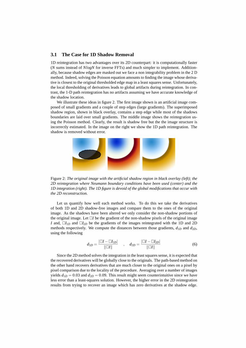
We illustrate these ideas in figure 2. The first image shown is an artificial image com-posed of small gradients and a couple of step edges (large gradients). The superimposedshadow region, shown in black overlay, contains a step edge while most of the shadowsboundaries are laid over small gradients. The middle image shows the reintegration us-ing the Poisson method. Clearly, the result is shadow free but the the image structure isincorrectly estimated. In the image on the right we show the 1D path reintegration. Theshadow is removed without error.

Figure 2:The original image with the artificial shadow region in black overlay (left); the2D reintegration where Neumann boundary conditions have been used (center) and the1D integration (right). The 1D figure is devoid of the global modifications that occur withthe 2D reconstruction.

Let us quantify how well each method works. To do this we take the derivativesof both 1D and 2D shadow-free images and compare them to the ones of the originalimage. As the shadows have been altered we only consider the non-shadow portions ofthe original image. Let∇I be the gradient of the non-shadow pixels of the original imageI and,∇I1D and∇I2D be the gradients of the images reintegrated with the 1D and 2Dmethods respectively. We compute the distances between those gradients,d1D andd2D,using the following

d1D =|∇I −∇I1D|

‖∇I‖, d2D =

|∇I −∇I2D|‖∇I‖

(6)

Since the 2D method solves the integration in the least squares sense, it is expected thatthe recovered derivatives will be globally close to the originals. The path-based method onthe other hand recovers derivatives that are much closer to the original ones on a pixel bypixel comparison due to the locality of the procedure. Averaging over a number of imagesyieldsd1D = 0.03 andd2D = 0.09. This result might seem counterintuitive since we haveless error than a least-squares solution. However, the higher error in the 2D reintegrationresults from trying to recover an image which has zero derivatives at the shadow edge.

The 1D we develop here (and discuss in the next section) works better because it ignoresthe detail (and derivatives) under the shadow edges.

4 Robust Shadow Removal

While the simple 1D method does indeed result in shadow-free images, they can alsocontain visually disturbing artifacts [4]. Those artifacts are introduced when an erroris committed in the reintegration. Since the shadow-free image is obtained by linearlyreintegrating the gradients, an error occurring at a timet1 will be propagated throughall timest > t1. The errors themselves are usually provoked by one of three factors: anincomplete shadow mask, the presence of a material edge or the presence of noise nearthe shadow edges.

The creation and propagation of artifacts is illustrated in figure 3, where the 1D graphsrepresent pixels in the image in their path-visited order. Figure 3a displays the ideal casewhere the non-shadow parts of the image are preserved and the shadow is effectively re-moved. If the shadow mask is not closed, which can happen since the shadow detectionmethod does not enforce closure, then a path can enter the shadow region through a de-tected shadow edge but then exit it through a “hole” in the edge map. Such a case is shownin figure 3b where one can appreciate the resulting error. Finally, when a material edgeis encountered at the same time than a shadow one or when noise is present, thresholdingthe gradient is incorrect as it supposes that both sides of the shadow edge are similar (i.e.would have the same values under identical lightning conditions). Figure 3c exemplifiesthe case where noise is present at the exit of the shadow region; the thresholded gradientdoes not take the noise into account and errors result. A further aspect to have in mind isthat the human eye is more sensitive to regular geometrical features [9]. Since the pathspreviously mentioned (raster and fractal) are all very regular, it makes sense to look forpaths having a more random structure as to minimize the visibility of artifacts.

Figure 3: Graph representation of the shadow regions of an image. (a) a perfect (sup-posed) reintegration. (b) Reintegration with errors due to an imperfect shadow mask. Theentry in the shadow region is well detected but the exit is not, thus creating a large error.(c) The noise/material edges case. The shadow edges are well detected, but the assump-tion of similarity is not enforced. Note how an error created at a point t1 in time is stillpropagated throughout all the pixels visited after a time t> t1.

To develop a robust framework for shadow removal, we address the various generatorsof errors present in the current algorithm. We first aim to close the shadow regions andthen proceed to minimize the number of crossings of the shadow edges in order lo limit

the influence of material edges and noise. More stable results can also be obtained byaveraging the output of a small number (say 4-5) of different paths. This does not inducea greater complexity since the most expensive steps of the algorithm (obtaining the maskand inpainting) are done once per image regardless of the number of paths.

4.1 Closing Shadow Edges

To close shadow edges we will use two different edge maps. The first one is obtainedby the method summarised in section 2.1 (by comparing the derivatives of the intrinsicand the full colour image). LetIS be this edge image. By constructionIS contains only(but possibly incomplete) shadow edges. The second edge map,IM, is obtained with themeanshift algorithm [10]. Meanshift segments images intoN regions and ensures that alledges are closed.

We then useIM as a guide to “complete” the edges ofIS. When an open point -no neighbour yet not along the image boundaries- is encountered inIS, we check whichregions ofIM are concerned (the ones having connecting edges). Among those regions,we select the one for whichIS edges span it the closest and complete said edge (see Fig. 4for illustration). We used this strategy on all of our edge maps and it consistently producedgood results.

Figure 4: From left to right: the original image, detected shadow edges IS, meanshiftedges IM and the resulting closure.

4.2 Random Hamiltonian Paths

The noise/material edge source of errors shown in figure 5c cannot be removed but we canminimize its occurrence. To do this, let us consider what happens when we reintegrate animage. Is is possible that when we enter a shadow, and so assume zero derivatives, thatthere is actually a material change (or simply noise). Suppose such an event happens withprobability perror. If we enter and exit a shadow regionN times, then the probability of atleast one error being propagated is 1− (1− perror)N, which tends to 1 whenN is large. Ifhowever by design we only enter and exit the shadow region once, the probability of errorpropagation isperror (for N ≥ 1, perror ≤ 1− (1− perror)N). Moreover, in our method wewill choose to reintegrate over a small number, say 4, of paths. In this case, the probabilityof all the paths being corrupted isp4

error (which is almost always close to zero).Reducing artifacts in the reintegrated image can therefore be achieved by both ran-

domizing the paths structure (necessary because simple patterns are visibly noticeable)and allowing a single crossing of the shadow edge. Allowing a single opening alter ourgraph in a way that the simple paths proposed in [4] and [8] are not usable anymore. Due

to the nature of our graph however, we know [11] that a random Hamiltonian path overour incomplete grid graph must exist. Indeed, probabilistic methods have been proposed[12] to find these paths but our graphs are relatively large and these methods take a greatdeal of time. So instead, we propose here a simple, deterministic and efficient methodwhose only requirement is that the image has to be of even size.

Let I be an image of sizen×m, where bothn andmare even. In the graph representa-tion, all valid pixels are nodes and all non valid ones (the shadow mask pixels) are holes inthe mesh. LetG be the original graph andGR the n

2 ×m2 graph obtained by downsampling

G. In GR, we create a single random connection between the shadow and non-shadowregions through the shadow edges. We then generate the minimum spanning treeT ofGR, where the randomization of the paths can be ensured by weightingGR with randomweights prior to generatingT. OnceT has been found, we “walk around” it, in a depth

Figure 5: (a) The spanning tree on GR and its walk around; (b) The corresponding treefor G and a possible Hamiltonian cycle. (c) The 4 different cases to turn a node of T into4 nodes of the upsampled tree. Depending on their degree, the nodes have more or less“inside connections”. Since these are the only possible degrees in our graphs, it is alwayspossible to derive an Hamiltonian cycle using such substitutions.

first way (see figure 5a for an illustration) until each edge has been visited twice. Doingso allow us to have the order list of nodes to visit to form a cycle. By constructionT is aspanning tree overGR but we are looking for a cycle onG. We can upsampleT by a factorof 2 and derive an Hamiltonian cycle overG. Figure 5c lists the different cases that canarise whenT is upsampled and it can be observed that we can always find such a cycle.The downsampled graphGR with the allowed random connection is strongly connected,which ensures that a minimum spanning tree will be found. Since we are working on gridgraphs, every node ofT, except the root, has a single parent and at most 3 child nodes.The root node has no parent and at most 4 child nodes. The upsampling/downsamplingprocedure implies that for each node inGR andT correspond 4 nodes inG andTU (theupsampled spanning tree). From the enumeration shown on figure 5c, it follows that onecan always obtain a cycle in the upsampled tree by substituting the nodes ofT for theones shown in fig. 5c. From a complexity point of view, the spanning tree can be com-puted inO(N) for our type of graphs and the substitution can be also done inO(N) bywalking aroundT and substituting the nodes depending on their degree. From a temporalpoint of view, a C++ version of the algorithm takes 0.3 seconds to calculate a path on a

1048×1048 graph.

4.3 Inpainting

Having obtained a proper shadow mask and a path, a shadow-free image can now be in-tegrated. Having allowed a single opening in the shadow mask, it follows that all othershadow edges pixels are not visited/reintegrated. The missing information can be inter-polated by various inpainting (sometimes called infilling) techniques. The most commonand fastest ones usually use the principle of diffusion to “grow back” missing regionsfrom their surroundings [13]. They unfortunately usually results in blurred regions thatare too noticeable for our purpose.

To prevent that, we use the method described in [14]. One first compute all possible11×11 windows for which all pixels are defined (not in the mask), letN be that number.Since the images are in and RGB-type space, each window has a size 11×11×3. Then,for each of the shadow mask pixels, a centered 11×11 window is used and its Euclidiandistance with respect to theN 11×11 windows in the image is computed. The windowcorresponding to the minimal Euclidian distance is then use to “fill in” the missing values.That is, the pixels values of the chosen window are directly copied at the “blank” pixelslocation. The procedure is then repeated until there are no more missing pixels.

5 Results

Figure 6 shows results obtained over a variety of images; the 1D results are the average ofthe output of 4 paths. Comparing the results obtained by the 2D and the 1D method onerealizes the improvement in quality of the latter, especially in colour rendition, despitehaving a simpler framework. Results are however not perfect. A non-exact shadow maskor the presence of colored noise in the image might alter the image gradient and perturbthe reintegration. This leads to shadow regions being a little “off-color” in some images,but this does not have a significant impact on the overall quality of the shadow-free im-ages.

6 Conclusion

To summarize, we have established a framework for robust reintegration of shadow-freeimages. We have addressed the different problems of both existing 1D and 2D methodsand proposed solutions to their shortcomings.

We have shown that a 1D approach was more suited to the task of shadow removaland that its results were more accurate than its 2D counterpart, while still being lesscomputationally expensive. We further devised solutions for existing 1D reintegrationusing the insights that shadow regions had to be closed and that the number of crossingsthrough the shadow edges should be limited. Additionally, we proposed a fast methodused to derive random Hamiltonian cycles in grid graphs. We finally proposed that non-visited shadow edge pixels do not have to be reintegrated and can simply be inpaintedonce the reintegration is complete.

To further enhance the quality of shadow removal, a better shadow detection methodwould prove useful. This particular aspect appears at the moment to be a bottleneck for

Figure 6:Typical results from shadow removal. The second line are results obtained withthe 2D method; the third line are results obtained with our path-based algorithm.

both quality and speed. Since the removal is directly dependant on the shadow mask, weare currently investigating novel techniques for robust and fast shadow detection.

Acknowledgments: Graham D. Finlayson gratefully acknowledges the support of theLeverhulme trust.

References[1] M. Turk and A. Pentland, “Face Recognition using Eigenfaces,”Proc. of the IEEE Conferenceon Computer Vision and Pattern Recognition (CVPR). 1991.[2] S. Ullman,High-Level Vision: Object recognition and Visual Cognition. MIT Press, 1996.[3] G. Finlayson, S. Hordley and M. Drew “Removing Shadows from Images,”Proc. of the IEEEEuropean Conference on Computer Vision (ECCV), 2002.[4] G. D. Finlayson and C. Fredembach “Fast Reintegration of Shadow Free Images,”Proc. of theIS& T 12th color Imaging Conference, 2004.[5] G. Finlayson, M. Drew and C. Lu, “Intrinsic Images by Entropy Minimization,”Proc. of theIEEE European Conference on Computer Vision (ECCV), 2004.[6] I. Stakgold,Green’s Functions and Boundary Value Problems. Wiley and Sons, 1979.[7] G. Finlayson and S. Hordley, “Color Constancy at a Pixel,”Journal of the Opt. Soc. of America.Vol 18, pp 253–264, 2001.[8] J.G. Griffiths, “An Algorithm for Displaying a Class of Space-Filling Curves,”Software: Prac-tice and Experience, Vol. 16, pp. 403–411, 1986.[9] B. Wandell,Foundations of Vision. Sinauer Associates, 1995.[10] D. Comanicu and P. Meer , “Mean shift: A robust approach toward feature space analysis,”IEEE Trans. Pattern Anal. Machine Intell. Vol 24, Nr. 5, pp 603–619, 2002.[11] E.L. Lawler, J.K. Lenstra, A.H.G. Rinnoy Kan and D.B. Shmoys,The Traveling SalesmanProblem. Wiley and Sons, 1986.[12] V. Chvatal, “Probabilistic methods in graph theory,”Annals of Operations Research. Vol 1, pp171–182, 1984.[13] M. Bertalmio et al. “Image Inpainting,”Proc. of SIGGRAPH, 2000.[14] A. Criminisi, P. Perez and K. Toyama, “Region Filling and Object Removal by Exemplar-BasedImage Inpainting,”IEEE Trans. on Image Processing. Vol 13, Nr. 9, pp 1200–1212, 2004.