haibing shao · philipp hein agnes sachse · olaf kolditz ... scenario ... b.2 msh: finite element...
TRANSCRIPT

S P R I N G E R B R I E F S I N E N E R G YCO M P U TAT I O N A L M O D E L I N G O F E N E R G Y S YS T E M S
Haibing Shao · Philipp HeinAgnes Sachse · Olaf Kolditz
Geoenergy Modeling II Shallow Geothermal Systems

SpringerBriefs in Energy
Computational Modeling of Energy Systems
Series Editors
Thomas NagelHaibing Shao
More information about this series at http://www.springer.com/series/8903

Haibing Shao • Philipp Hein • Agnes SachseOlaf Kolditz
Geoenergy Modeling IIShallow Geothermal Systems
123

Haibing ShaoDepartment of Environmental InformaticsHelmholtz Centre for Environmental
ResearchLeipzig, Germany
Agnes SachseDepartment of Environmental
InformaticsHelmholtz Centre of Environmental
Research-UFZLeipzig, Germany
Philipp HeinHelmholtz Centre of Environmental
Research UFZDepartment of Environmental
InformaticsUniversity of Applied Science Leipzig
HTWKFaculty of Mechanical and Energy
EngineeringLeipzig, Germany
Olaf KolditzEnvironmental InformaticsHelmholtz-Zentrum für Umweltforschu
Environmental InformaticsLeipzig, Sachsen, Germany
ISSN 2191-5520 ISSN 2191-5539 (electronic)SpringerBriefs in EnergyISBN 978-3-319-45055-1 ISBN 978-3-319-45057-5 (eBook)DOI 10.1007/978-3-319-45057-5
Library of Congress Control Number: 2016935862
© The Author(s) 2016This work is subject to copyright. All rights are reserved by the Publisher, whether the whole or part ofthe material is concerned, specifically the rights of translation, reprinting, reuse of illustrations, recitation,broadcasting, reproduction on microfilms or in any other physical way, and transmission or informationstorage and retrieval, electronic adaptation, computer software, or by similar or dissimilar methodologynow known or hereafter developed.The use of general descriptive names, registered names, trademarks, service marks, etc. in this publicationdoes not imply, even in the absence of a specific statement, that such names are exempt from the relevantprotective laws and regulations and therefore free for general use.The publisher, the authors and the editors are safe to assume that the advice and information in this bookare believed to be true and accurate at the date of publication. Neither the publisher nor the authors orthe editors give a warranty, express or implied, with respect to the material contained herein or for anyerrors or omissions that may have been made.
Printed on acid-free paper
This Springer imprint is published by Springer NatureThe registered company is Springer International Publishing AGThe registered company address is Gewerbestrasse 11, 6330 Cham, Switzerland

Foreword
This tutorial presents the introduction of the open-source software OpenGeoSys(OGS) for shallow geothermal applications. This tutorial is the result of a closecooperation within the OGS community (www.opengeosys.org). These voluntarycontributions are highly acknowledged.
The book contains general information regarding the numerical simulation ofheat transport process in the shallow subsurface, which is closely coupled withthe operation of borehole heat exchangers (BHE) and ground source heat pumps(GSHP). In addition to the introduction of how to establish such a model, benchmarkexamples and a real-world test case is presented in this book, which leads to concreteadvices for the end users when exploring shallow geothermal energy.
This book is intended primarily for graduate students and applied scientists whodeal with geothermal system analysis. It is also a valuable source of informationfor professional geoscientists wishing to advance their knowledge in numericalmodeling of geothermal processes, including convection and conduction. As such,this book will be a valuable help in geothermal modeling training courses.
There are various commercial software tools available to solve complex scientificquestions in geothermics. This book will introduce the user to an open-sourcenumerical software code for geothermal modeling which can even be adapted andextended based on the needs of the researcher.
This tutorial is part of a series that will represent further applications ofcomputational modeling in energy sciences. Within this series, the planned tutorialsrelated to the specific simulation platform OGS. The planned tutorials are:
• OpenGeoSys Tutorial. Basics of Heat Transport Processes in Geothermal Sys-tems, Böttcher et al. (2015)
• OpenGeoSys Tutorial. Shallow Geothermal Systems, Shao et al. (2016), thisvolume
• OpenGeoSys Tutorial. Enhanced Geothermal Systems, Watanabe et al. (2016*)• OpenGeoSys Tutorial. Geotechnical Storage of Energy Carriers, Böttcher et al.
(2016*)
v

vi Foreword
• OpenGeoSys Tutorial. Models of Thermochemical Heat Storage, Nagel et al.(2017*)
These contributions are related to a similar publication series in the field ofenvironmental sciences, namely:
• Computational Hydrology I: Groundwater flow modeling, Sachse et al.(2015), DOI 10.1007/978-3-319-13335-5, http://www.springer.com/de/book/9783319133348
• OpenGeoSys Tutorial. Computational Hydrology II: Density-dependent flow andtransport processes, Walther et al. (2016*)
• OGS Data Explorer, Rink et al. (2016*)• Reactive Transport Modeling I (2017*)• Multiphase Flow (2017*)
(*publication time is approximated).
Leipzig, Germany Haibing ShaoJune 2016 Philipp Hein
Agnes SachseOlaf Kolditz

Acknowledgments
We deeply acknowledge the continuous scientific and financial support to theOpenGeoSys development activities by the following institutions:
We would like to express our sincere thanks to HIGRADE in providing fundingfor the OpenGeoSys training course at the Helmholtz Centre for EnvironmentalResearch.
We also wish to thank the OpenGeoSys developer group ([email protected]) and the users ([email protected]) for their technical support.
vii

Contents
1 Introduction . . . . . . . . . . . . . . . . . . . . . . . . . . . . . . . . . . . . . . . . . . . . . . . . . . . . . . . . . . . . . . . . . . . 11.1 Geothermal Systems . . . . . . . . . . . . . . . . . . . . . . . . . . . . . . . . . . . . . . . . . . . . . . . . . . . 11.2 Geothermal Resources . . . . . . . . . . . . . . . . . . . . . . . . . . . . . . . . . . . . . . . . . . . . . . . . . 21.3 Utilizing Shallow Geothermal Resources . . . . . . . . . . . . . . . . . . . . . . . . . . . . . 31.4 Tutorial and Course Structure . . . . . . . . . . . . . . . . . . . . . . . . . . . . . . . . . . . . . . . . . 5
2 Theory: Governing Equations and Model Implementations . . . . . . . . . . . . . 72.1 Conceptual Model of the BHEs . . . . . . . . . . . . . . . . . . . . . . . . . . . . . . . . . . . . . . . 72.2 Governing Equations . . . . . . . . . . . . . . . . . . . . . . . . . . . . . . . . . . . . . . . . . . . . . . . . . . . 9
2.2.1 Governing Equations for the Heat TransportProcess in Soil . . . . . . . . . . . . . . . . . . . . . . . . . . . . . . . . . . . . . . . . . . . . . . . . 9
2.2.2 Governing Equations for the Borehole Heat Exchangers . . . 92.2.3 Calculation of the Cauchy Type of Boundary Conditions . . 10
2.3 Numerical Model . . . . . . . . . . . . . . . . . . . . . . . . . . . . . . . . . . . . . . . . . . . . . . . . . . . . . . . 102.3.1 Mesh Arrangement . . . . . . . . . . . . . . . . . . . . . . . . . . . . . . . . . . . . . . . . . . . 102.3.2 Finite Element Discretization . . . . . . . . . . . . . . . . . . . . . . . . . . . . . . . . 122.3.3 Assembly of the Global Equation System. . . . . . . . . . . . . . . . . . . 152.3.4 Picard Iterations and Time Stepping Schemes . . . . . . . . . . . . . . 16
3 OGS Project: Simulating Heat Transport Model with BHEs . . . . . . . . . . . . 193.1 Download and Compile the Source Code . . . . . . . . . . . . . . . . . . . . . . . . . . . . . 19
3.1.1 Download the Source Code . . . . . . . . . . . . . . . . . . . . . . . . . . . . . . . . . . 193.1.2 Using CMake to Configure the Building Project. . . . . . . . . . . . 213.1.3 Compiling the Code . . . . . . . . . . . . . . . . . . . . . . . . . . . . . . . . . . . . . . . . . . 22
3.2 Define Heat Transport Process with BHEs. . . . . . . . . . . . . . . . . . . . . . . . . . . . 243.2.1 Process Definition . . . . . . . . . . . . . . . . . . . . . . . . . . . . . . . . . . . . . . . . . . . . 243.2.2 Deactivated Sub-domains . . . . . . . . . . . . . . . . . . . . . . . . . . . . . . . . . . . . 253.2.3 Primary Variables . . . . . . . . . . . . . . . . . . . . . . . . . . . . . . . . . . . . . . . . . . . . . 25
3.3 Geometry of BHEs . . . . . . . . . . . . . . . . . . . . . . . . . . . . . . . . . . . . . . . . . . . . . . . . . . . . . 253.4 Mesh of BHEs . . . . . . . . . . . . . . . . . . . . . . . . . . . . . . . . . . . . . . . . . . . . . . . . . . . . . . . . . . 263.5 Parameters of BHEs . . . . . . . . . . . . . . . . . . . . . . . . . . . . . . . . . . . . . . . . . . . . . . . . . . . . 273.6 Initial Conditions for the BHE. . . . . . . . . . . . . . . . . . . . . . . . . . . . . . . . . . . . . . . . . 31
ix

x Contents
3.7 Boundary Conditions for the BHE . . . . . . . . . . . . . . . . . . . . . . . . . . . . . . . . . . . . 323.8 Output of Temperatures . . . . . . . . . . . . . . . . . . . . . . . . . . . . . . . . . . . . . . . . . . . . . . . . 333.9 Running the OGS Model . . . . . . . . . . . . . . . . . . . . . . . . . . . . . . . . . . . . . . . . . . . . . . 333.10 Visualization of Temperature Evolution . . . . . . . . . . . . . . . . . . . . . . . . . . . . . . 35
3.10.1 Visualization of Soil Temperatures . . . . . . . . . . . . . . . . . . . . . . . . . . 353.10.2 Visualization of BHE Temperatures . . . . . . . . . . . . . . . . . . . . . . . . . 36
4 BHE Meshing Tool . . . . . . . . . . . . . . . . . . . . . . . . . . . . . . . . . . . . . . . . . . . . . . . . . . . . . . . . . . . . 394.1 Requirement on the Mesh. . . . . . . . . . . . . . . . . . . . . . . . . . . . . . . . . . . . . . . . . . . . . . 404.2 Input File for the Meshing Tool . . . . . . . . . . . . . . . . . . . . . . . . . . . . . . . . . . . . . . . 404.3 Output. . . . . . . . . . . . . . . . . . . . . . . . . . . . . . . . . . . . . . . . . . . . . . . . . . . . . . . . . . . . . . . . . . . 42
5 Benchmarks . . . . . . . . . . . . . . . . . . . . . . . . . . . . . . . . . . . . . . . . . . . . . . . . . . . . . . . . . . . . . . . . . . . 475.1 Borehole Heat Exchangers: Comparison to Line Source Model . . . . . 47
5.1.1 ILS Analytical Solution . . . . . . . . . . . . . . . . . . . . . . . . . . . . . . . . . . . . . . 485.1.2 Numerical Line Source Model . . . . . . . . . . . . . . . . . . . . . . . . . . . . . . . 485.1.3 Numerical BHE Model . . . . . . . . . . . . . . . . . . . . . . . . . . . . . . . . . . . . . . . 495.1.4 Results . . . . . . . . . . . . . . . . . . . . . . . . . . . . . . . . . . . . . . . . . . . . . . . . . . . . . . . . 52
5.2 Borehole Heat Exchangers: Comparison to Sandbox Experiment . . . 525.2.1 Model Setup . . . . . . . . . . . . . . . . . . . . . . . . . . . . . . . . . . . . . . . . . . . . . . . . . . 545.2.2 OGS Input Files . . . . . . . . . . . . . . . . . . . . . . . . . . . . . . . . . . . . . . . . . . . . . . 555.2.3 Results . . . . . . . . . . . . . . . . . . . . . . . . . . . . . . . . . . . . . . . . . . . . . . . . . . . . . . . . 59
6 Case Study: A GSHP System in the Leipzig Area . . . . . . . . . . . . . . . . . . . . . . . . . 616.1 The Leipzig-Area Model. . . . . . . . . . . . . . . . . . . . . . . . . . . . . . . . . . . . . . . . . . . . . . . 61
6.1.1 Scenario . . . . . . . . . . . . . . . . . . . . . . . . . . . . . . . . . . . . . . . . . . . . . . . . . . . . . . . 616.1.2 BHE Design . . . . . . . . . . . . . . . . . . . . . . . . . . . . . . . . . . . . . . . . . . . . . . . . . . 626.1.3 Model Domain . . . . . . . . . . . . . . . . . . . . . . . . . . . . . . . . . . . . . . . . . . . . . . . . 626.1.4 Initial and Boundary Conditions . . . . . . . . . . . . . . . . . . . . . . . . . . . . . 636.1.5 Input Files . . . . . . . . . . . . . . . . . . . . . . . . . . . . . . . . . . . . . . . . . . . . . . . . . . . . . 646.1.6 Geometry. . . . . . . . . . . . . . . . . . . . . . . . . . . . . . . . . . . . . . . . . . . . . . . . . . . . . . 646.1.7 Process Definition . . . . . . . . . . . . . . . . . . . . . . . . . . . . . . . . . . . . . . . . . . . . 666.1.8 Numerical Properties . . . . . . . . . . . . . . . . . . . . . . . . . . . . . . . . . . . . . . . . . 666.1.9 Time Discretization. . . . . . . . . . . . . . . . . . . . . . . . . . . . . . . . . . . . . . . . . . . 676.1.10 Initial and Boundary Conditions . . . . . . . . . . . . . . . . . . . . . . . . . . . . . 676.1.11 Data RFD File . . . . . . . . . . . . . . . . . . . . . . . . . . . . . . . . . . . . . . . . . . . . . . . . 706.1.12 Fluid Properties . . . . . . . . . . . . . . . . . . . . . . . . . . . . . . . . . . . . . . . . . . . . . . . 726.1.13 Solid Phase Properties . . . . . . . . . . . . . . . . . . . . . . . . . . . . . . . . . . . . . . . . 726.1.14 Medium Properties . . . . . . . . . . . . . . . . . . . . . . . . . . . . . . . . . . . . . . . . . . . 73
6.2 Simulation Results . . . . . . . . . . . . . . . . . . . . . . . . . . . . . . . . . . . . . . . . . . . . . . . . . . . . . 756.3 Implifications of the Model . . . . . . . . . . . . . . . . . . . . . . . . . . . . . . . . . . . . . . . . . . . . 77
6.3.1 Overall Dynamics of the BHE Coupled GSHP System . . . . 776.3.2 The Role of the Heat Pump . . . . . . . . . . . . . . . . . . . . . . . . . . . . . . . . . . 776.3.3 The Price of Under-Design. . . . . . . . . . . . . . . . . . . . . . . . . . . . . . . . . . . 78

Contents xi
7 Summary and Outlook . . . . . . . . . . . . . . . . . . . . . . . . . . . . . . . . . . . . . . . . . . . . . . . . . . . . . . . 81
A Symbols . . . . . . . . . . . . . . . . . . . . . . . . . . . . . . . . . . . . . . . . . . . . . . . . . . . . . . . . . . . . . . . . . . . . . . . . 83
B Keywords . . . . . . . . . . . . . . . . . . . . . . . . . . . . . . . . . . . . . . . . . . . . . . . . . . . . . . . . . . . . . . . . . . . . . . 85B.1 GLI: Geometry . . . . . . . . . . . . . . . . . . . . . . . . . . . . . . . . . . . . . . . . . . . . . . . . . . . . . . . . . 85B.2 MSH: Finite Element Mesh. . . . . . . . . . . . . . . . . . . . . . . . . . . . . . . . . . . . . . . . . . . . 85B.3 PCS: Process Definition . . . . . . . . . . . . . . . . . . . . . . . . . . . . . . . . . . . . . . . . . . . . . . . 86B.4 NUM: Numerical Properties . . . . . . . . . . . . . . . . . . . . . . . . . . . . . . . . . . . . . . . . . . . 86B.5 TIM: Time Discretization . . . . . . . . . . . . . . . . . . . . . . . . . . . . . . . . . . . . . . . . . . . . . . 87B.6 IC: Initial Conditions. . . . . . . . . . . . . . . . . . . . . . . . . . . . . . . . . . . . . . . . . . . . . . . . . . . 88B.7 BC: Boundary Conditions . . . . . . . . . . . . . . . . . . . . . . . . . . . . . . . . . . . . . . . . . . . . . 88B.8 ST: Source/Sink Terms. . . . . . . . . . . . . . . . . . . . . . . . . . . . . . . . . . . . . . . . . . . . . . . . . 89B.9 MFP: Fluid Properties . . . . . . . . . . . . . . . . . . . . . . . . . . . . . . . . . . . . . . . . . . . . . . . . . 89B.10 MSP: Solid Properties . . . . . . . . . . . . . . . . . . . . . . . . . . . . . . . . . . . . . . . . . . . . . . . . . 90B.11 MMP: Porous Medium Properties . . . . . . . . . . . . . . . . . . . . . . . . . . . . . . . . . . . . . 90B.12 OUT: Output Parameters. . . . . . . . . . . . . . . . . . . . . . . . . . . . . . . . . . . . . . . . . . . . . . . 91
References . . . . . . . . . . . . . . . . . . . . . . . . . . . . . . . . . . . . . . . . . . . . . . . . . . . . . . . . . . . . . . . . . . . . . . . . . . 93

List of Contributors
Philipp Hein, Faculty of Mechanical and Energy Engineering, University ofApplied Science Leipzig – HTWK, Leipzig, Germany
Department of Environmental Informatics, Helmholtz Centre of EnvironmentalResearch – UFZ, Leipzig, Germany
Olaf Kolditz, Department of Environmental Informatics, Helmholtz Centre ofEnvironmental Research – UFZ, Leipzig, Germany
Applied Environmental System Analysis, Technical University of Dresden, Dres-den, Germany
Agnes Sachse, Department of Environmental Informatics, Helmholtz Centre ofEnvironmental Research – UFZ, Leipzig, Germany
Haibing Shao, Department of Environmental Informatics, Helmholtz Centre ofEnvironmental Research – UFZ, Leipzig, Germany
Faculty of Geoscience, Geotechnics and Mining, Freiberg University of Mining andTechnology – TUBAF, Freiberg, Germany
xiii

Chapter 1Introduction
1.1 Geothermal Systems
Geothermal energy is a promising alternative energy source as it is suited for base-loadenergy supply, can replace fossil fuel power generation, can be combined with otherrenewable energy sources such as solar thermal energy, and can stimulate the regionaleconomy.
The above text is quoted from an editorial of a new open-access journal Geother-mal Energy (Kolditz et al. 2013), which advocates the potential of this renewableenergy resource for both heat supply and electricity production. Indeed, Geothermalenergy has recently became an essential part in many research programmes world-wide. The current status of research on geoenergy (including both geological energyresources and concepts for energy waste deposition) in Germany and other countrieshas been compiled in a thematic issue on “Geoenergy: new concepts for utilizationof geo-reservoirs as potential energy sources” (Scheck-Wenderoth et al. 2013). TheHelmholtz Association dedicated a topic on geothermal energy systems into its next5-year-program from 2015 to 2019 (Huenges et al. 2013).
When looking at different types of geothermal systems, it can be distinguishedbetween shallow, medium, and deep systems in general (cf. Fig. 1.1). Installationsof shallow systems are allowed down to 100–150 m of subsurface, which includessoil and shallow aquifers. If going further down, the medium systems are associatedwith hydrothermal resources and may be suited for underground thermal storage(Bauer et al. 2013). Deep systems are connected to petrothermal sources and needto be stimulated, in order to increase the hydraulic conductivity for heat extractionby fluid circulation (Enhanced Geothermal Systems—EGS).
© The Author(s) 2016H. Shao et al., Geoenergy Modeling II, SpringerBriefs in Energy,DOI 10.1007/978-3-319-45057-5_1
1

2 1 Introduction
Fig. 1.1 Overview of different types of geothermal systems: shallow, medium and deep systems(Huenges et al. 2013)
1.2 Geothermal Resources
In general, the corresponding temperature regimes at different depths dependon the geothermal gradient (Clauser 1999). Some areas benefit from favourablegeothermal conditions with amplified heat fluxes, e.g., in the North German Basin,Upper Rhine Valley, and the Molasse Basin of Germany (Cacace et al. 2013).Conventional geothermal systems mainly rely on heated water (hydrothermalsystems) that approaches the near-surface. Therefore they are regionally limitedto near continental plate boundaries and volcanoes. Nevertheless, this book willfocus on the numerical modelling of extracting shallow geothermal resources. Inparticular, this book will explain in details how to numerically simulate the evolvingsoil temperature in response to heat extraction from borehole heat exchangers.
Before diving down into the numerical world, let’s have an overview on howmuch energy is stored in the subsurface that we are standing on. First, here are someinteresting numbers about the solid earth:
• The mean surface temperature is abut 15 ıC.• Despite of strong fluctuations of the surface temperature, the soil or rock
temperature beneath 15–20 m of depth is largely constant.• The geothermal gradient in the upper part is about 30 K per kilometer depth
(0.03 Km�1). In another word, from the surface downwards, the average soiltemperature will increase 3ı by every 100 m.
So how much energy can we extract from the shallow subsurface?

1.3 Utilizing Shallow Geothermal Resources 3
When looking into the shallow geothermal systems, it is rather unlikely to havea 20–30 K temperature drop as in the deep geothermal reservoirs. However, if thetemperature of the shallow subsurface is decreased by only 0.5–2 ıC, it will stillgenerate large amount of energy. For example, Zhu et al. (2010) evaluated thegeothermal potential of the city Cologne, and they found that a temperature decreaseof 2 ıC in the 20 m thick aquifer will yield enough energy that is more than the city’sannual space heating demand. Using a similar approach, Arola and Korkka-Niemi(2014) assessed the effect of urban heat islands on the geothermal potential in threecities in southern Finland. It turns out that, because of the urban heat island effect,50–60 % more heat can be supplied from shallow subsurface in the urban area, incomparison to rural areas.
1.3 Utilizing Shallow Geothermal Resources
Now the energy embedded in the shallow subsurface is more than plenty. How can itbe utilized? Currently, the most widely applied technology is the so-called GroundSource Heat Pump (GSHP) system. Such system is typically composed of threeinter-connected parts (cf. Fig. 1.2), namely (1) the ground loop, (2) the heat pump,and (3) the in-door loop.
Heat Pump
Buffer Tank
CirculatingFluid Pump
Floor Heating
Hot Water Supply
considered in the model
not yet included in the model
direct BHE boundary condition
COP correctedboundary condition
Soil
filled withgrout
Fig. 1.2 Overview of the Ground Source Heat Pump (GSHP) system, reproduced after Zhenget al. (2016)

4 1 Introduction
• The ground loop is composed of one or multiple borehole heat exchangers(BHE). Their main function is to extract heat from the shallow subsurface forbuilding heating, or injecting heat while providing cooling. This is typicallyachieved by installing closed loop tubes, buried vertically or horizontally in theground, and circulating refrigerant through the pipes.
• The function of the heat pump, is to elevate the low-grade heat from the groundloop, to high-grade heat that can directly be applied for room heating or hot watersupply.
• As for the in-door loop, it is designed to transport and dissipate high-grade heator code through the building.
In this book, the numerical modelling software OpenGeoSys (OGS) will beemployed to model the borehole heat exchanger and heat pump part, more specifi-cally to simulate the dynamics behaviour of soil temperature due to GSHP operation(Fig. 1.3).
Fig. 1.3 THMC coupling concept. OGS is a scientific open-source initiative for numericalsimulation of thermo-hydro-mechanical/chemical (THMC) processes in porous and fracturedmedia, continuously developed since the mid-eighties. The OGS code is targeting primarilyapplications in environmental geoscience, e.g. in the fields of contaminant hydrology, waterresources management, waste deposits, or geothermal systems, but it has also been applied tonew topics in energy storage recently

1.4 Tutorial and Course Structure 5
1.4 Tutorial and Course Structure
This tutorial “Computational Energy Systems II: Shallow Geothermal System”contains several parts. In Chap. 2, the governing equations of the numerical modelwill be defined. Chapter 3 shows the user how to set up a project to simulateheat transport processes induced by a BHE operation. To construct the mesh usedin Chap. 3, a meshing tool will be needed, which is introduced in Chap. 4. Thedeveloped OGS model will be verified in Chap. 5, with three different benchmarks.A realistic application is presented in Chap. 6, and the knowledge from the mod-elling study will be further discussed. This tutorial can also be used in combinationwith the following material
• OGS training course on geoenergy aspects held by Norihiro Watanabe inNovember 2013 in Guangzhou,
• OGS training course on CO2-reduction modelling held by Norbert Böttcher in2012 in Daejon, South Korea,
• OGS benchmarking chapter on heat transport processes by Norbert Böttcher,• University lecture material (TU Dresden) and presentations by Olaf Kolditz.
By visiting the OGS webpage at https://docs.opengeosys.org/books/shallow-geothermal-systems, interested readers can obtain the dataset used in this book,to conduct their own simulations for the ground source heat pump system.

Chapter 2Theory: Governing Equations and ModelImplementations
Here in this chapter of the tutorial, the governing equations of heat transportprocesses inside and around the Borehole Heat Exchangers (BHEs) will be pre-sented. Also, discussions will focus on the numerical techniques applied in Open-GeoSys to solve it. Note that the method implemented here is not the creative workof the authors, but rather a collection of contributions from the scientific community.The formulation of heat exchange between BHEs and the surrounding soil, wasproposed by Al-Khoury et al. (2010). This formulation was later-on adopted byDiersch et al. (2011a,b) into the commercial software FEFLOW. In this work,the same idea of Al-Khoury and Diersch was implemented into the open-sourcescientific software OpenGeoSys, to simulate the heat transport process in responseto BHEs. For interested readers, the FEFLOW book (Diersch 2014) also provides agood reference for the better understanding of the Finite Element Method (FEM).
2.1 Conceptual Model of the BHEs
To exchange heat with the surrounding soil and rock, borehole heat exchangersare installed in the subsurface. They have different designs and configurations. Themost commonly applied BHEs are four different types, including the single U-tube(1U), double U-tube (2U), coaxial centred (CXC) and coaxial annular (CXA) types.The U-type BHEs are named after the U shaped pipelines laid vertically alongthe borehole. The number 1 or 2 refer to how many pairs of U tubes are in thesame borehole. To illustrate this, Fig. 2.1 shows the horizontal cross-section of a 1Utype BHE. Notice that the U tubes are normally sealed by grout materials, and notin direct contact with the soil. For a typical BHE, a refrigerant fluid is circulatinginside of the U tube, absorbing or releasing heat from or into the surrounding groutand soil.
© The Author(s) 2016H. Shao et al., Geoenergy Modeling II, SpringerBriefs in Energy,DOI 10.1007/978-3-319-45057-5_2
7

8 2 Theory: Governing Equations and Model Implementations
Tg1 Tg2
Ts
Ts
Ti1To1
w
D
Tg1 Tg2
Ti1 To1
Ts
Cg Cg
Rfig Rfog
Rgg
Rgs Rgs
Fig. 2.1 Configuration of the 1U type BHE and its corresponding resister-capacitor concept,reproduced after the FEFLOW book Diersch (2014)
In order to numerically simulate the heat transfer process inside a BHE, thedevice is further conceptualized by the so-called Resister-Capacitor model. Thisidea originates from the discipline of electrical engineering. In a electrical circuit,if the electric current is hindered by a component, it is called a Resistor. When acomponent is capable of storing the electricity, then it is named as a Capacitor. So thesame concept can also be applied to the heat transport in a BHE. Taking the 1U typeof BHE in Fig. 2.1 as an example, four temperature values are assigned to differentcompartments. They are Ts, Ti1, To1, Tg1 and Tg2, referring to the temperatures of thesurrounding soil, the inlet pipe, the outlet pie, the fisrt (left) and the second (right)grout zone respectively. As a convention, it is always assumed that the first groutzone is the one surrounding the inlet pipe. Following this concept, the heat transferbetween the pipe and the soil can be divided into five pathways: (1) between inletpipe and first grout zone; (2) between outlet pipe and second grout zone; (3) betweenthe two grout zones; (4) between first grout zone and the soil; (5) between secondgrout zone and the soil. The heat flux qn on each of these pathways, are drivenby the temperature difference and regulated by the heat transfer coefficient ˚ . Forexample, the heat flux from inlet pipe to the first grout zone can be calculated by
qn D ˚fig�Ti1 � Tg1
�; (2.1)
in which the heat transfer coefficient˚ is inversely dependent on the product of heatresistance R and specific exchange area S
˚ D 1
RS(2.2)

2.2 Governing Equations 9
Depending on the pathway, there will be different heat transfer coefficients, denotedas ˚fig, ˚fog, ˚gg and ˚gs. Details regarding how to calculate these heat transfercoefficients can be found in Diersch et al. (2011a).
2.2 Governing Equations
2.2.1 Governing Equations for the Heat TransportProcess in Soil
For the heat transport process in the soil, the development of soil temperature Ts
is contributed by both the heat convection of the fluid f in the soil and the heatconduction through the soil matrix. Let �s, �f and cs, cf be the density and specificheat capacity of fluid f and soil s. If assuming the soil matrix is fully saturated withgroundwater, the Darcy velocity of which is described by the vector v, then theconservation equation writes as
@
@t
���f cf C .1 � �/�scs
�Ts C r � ��f cf vTs
� � r � .�s � rTs/ D Hs; (2.3)
with �s the tensor of thermal hydrodynamic dispersion and Hs the source and sinkterms for heat. When considering the heat exchange between the BHEs and the soil,the above governing equation is subject to a Cauchy-type of boundary condition:
� .�s � rTs/ D qnTs : (2.4)
2.2.2 Governing Equations for the Borehole Heat Exchangers
The governing equations for the BHE write differently, depending on whether it isfor the pipelines or for the grout zones. Let ˝k refer to the different compartmentsin the BHE. For the pipelines (k D i1; o1), the heat transport process is dominatedby the convection of the refrigerant r with a flow rate u.
�rcr @Tk
@tC �rcru � rTk � r � .�r � rTk/ D Hk in ˝k
with Cauchy type of BC W � .�r � rTk/ � n D qnTk on �k
for k D i1; o1; .i2; o2/ (2.5)
�r stands for the hydrodynamic thermo-dispersion of the refrigerant,
�r D .�r C �rcrˇLkuk/ ı: (2.6)
10 2 Theory: Governing Equations and Model Implementations
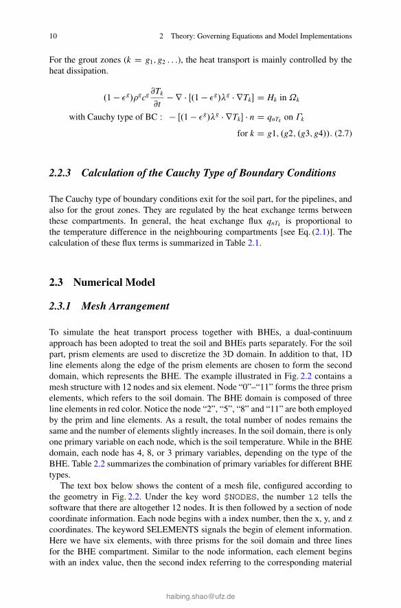
For the grout zones (k D g1; g2 : : :), the heat transport is mainly controlled by theheat dissipation.
.1 � �g/�gcg @Tk
@t� r � Œ.1 � �g/�g � rTk� D Hk in ˝k
with Cauchy type of BC W � Œ.1 � �g/�g � rTk� � n D qnTk on �k
for k D g1; .g2; .g3; g4//: (2.7)
2.2.3 Calculation of the Cauchy Type of Boundary Conditions
The Cauchy type of boundary conditions exit for the soil part, for the pipelines, andalso for the grout zones. They are regulated by the heat exchange terms betweenthese compartments. In general, the heat exchange flux qnTk is proportional tothe temperature difference in the neighbouring compartments [see Eq. (2.1)]. Thecalculation of these flux terms is summarized in Table 2.1.
2.3 Numerical Model
2.3.1 Mesh Arrangement
To simulate the heat transport process together with BHEs, a dual-continuumapproach has been adopted to treat the soil and BHEs parts separately. For the soilpart, prism elements are used to discretize the 3D domain. In addition to that, 1Dline elements along the edge of the prism elements are chosen to form the seconddomain, which represents the BHE. The example illustrated in Fig. 2.2 contains amesh structure with 12 nodes and six element. Node “0”–“11” forms the three prismelements, which refers to the soil domain. The BHE domain is composed of threeline elements in red color. Notice the node “2”, “5”, “8” and “11” are both employedby the prim and line elements. As a result, the total number of nodes remains thesame and the number of elements slightly increases. In the soil domain, there is onlyone primary variable on each node, which is the soil temperature. While in the BHEdomain, each node has 4, 8, or 3 primary variables, depending on the type of theBHE. Table 2.2 summarizes the combination of primary variables for different BHEtypes.
The text box below shows the content of a mesh file, configured according tothe geometry in Fig. 2.2. Under the key word $NODES, the number 12 tells thesoftware that there are altogether 12 nodes. It is then followed by a section of nodecoordinate information. Each node begins with a index number, then the x, y, and zcoordinates. The keyword $ELEMENTS signals the begin of element information.Here we have six elements, with three prisms for the soil domain and three linesfor the BHE compartment. Similar to the node information, each element beginswith an index value, then the second index referring to the corresponding material

2.3 Numerical Model 11
Table 2.1 Boundary heat fluxes qnTk for different types of BHEs, reproduced after theFEFLOW book (Diersch 2014)
k 2U 1U CXA CXC
i1 �˚2Ufig .Tg1 � Ti1/ �˚1U
fig .Tg1 � Ti1/ �˚CXAfig .Tg1 � Ti1/ �˚CXC
ff .To1 � Ti1/
�˚CXAff .To1 � Ti1/
i2 �˚2Ufig .Tg2 � Ti2/ – – –
o1 �˚2Ufog .Tg3 � To1/ �˚1U
fog .Tg2 � To1/ �˚CXAff .Ti1 � To1/ �˚CXC
fog .Tg1 � To1/
�˚CXCff .Ti1 � To1/
o2 �˚2Ufog .Tg4 � To2/ – – –
g1 �˚2Ugs .Ts � Tg1/ �˚1U
gs .Ts � Tg1/ �˚CXCgs .Ts � Tg1/ �˚CXA
gs .Ts � Tg1/
�˚2Ufig .Ti1 � Tg1/ �˚1U
fig .Ti1 � Tg1/ �˚CXCfog .To1 � Tg1/ �˚CXA
gs .Ts � Tg1/
�˚2Ugg2.Tg2 � Tg1/ �˚1U
gg .Tg2 � Tg1/ – –
�˚2Ugg1.Tg3 � Tg1/
�˚2Ugg1.Tg4 � Tg1/
g2 �˚2Ugs .Ts � Tg2/ �˚1U
gs .Ts � Tg2/
�˚2Ufig .Ti2 � Tg2/ �˚1U
fog .To1 � Tg2/
�˚2Ugg2.Tg1 � Tg2/ �˚1U
gg .Tg1 � Tg2/ – –
�˚2Ugg1.Tg3 � Tg2/
�˚2Ugg1.Tg4 � Tg2/
g3 �˚2Ugs .Ts � Tg3/
�˚2Ufig .To1 � Tg3/
�˚2Ugg2.Tg4 � Tg3/ – – –
�˚2Ugg1.Tg1 � Tg3/
�˚2Ugg1.Tg2 � Tg3/
g4 �˚2Ugs .Ts � Tg4/
�˚2Ufig .To2 � Tg4/
�˚2Ugg2.Tg3 � Tg4/ – – –
�˚2Ugg1.Tg1 � Tg4/
�˚2Ugg1.Tg2 � Tg4/
properties. The keywords pris and line denotes the type of the element, followedby the index of nodes that are connected to this element.
Listing 2.1 Mesh File
#FEM_MSH$PCS_TYPEHEAT_TRANSPORT_BHE$NODES120 0 0 01 0 1 02 1 0 03 0 1 14 0 0 15 1 0 16 0 1 27 0 0 28 1 0 29 0 1 3

12 2 Theory: Governing Equations and Model Implementations
10 0 0 311 1 0 3$ELEMENTS60 0 pris 2 1 0 5 3 41 0 pris 5 3 4 8 6 72 0 pris 8 6 7 11 9 103 1 line 9 64 1 line 6 35 1 line 3 1#STOP
2.3.2 Finite Element Discretization
For the domain of BHEs, the governing Eqs. (2.5) and (2.7) are discretized by finiteelements. By introducing the spatial weighting function !, the weak statementswrite as
Ti1
N#0
N#1
N#2
N#5
N#8
N#11
N#9
N#10N#6
N#7
N#4
N#3
Ti1To1
To1
Tg1
Tg2
Tg2
Tg1
Tg1
Fig. 2.2 Mesh and geometry structure, with soil domain represented by prism elements and BHEby line elements
Table 2.2 Different combination of primary variables for the borehole heat exchangers
Type of BHE Number of primary variables Combination of primary variables
1U 4 Ti1; To1; Tg1; Tg2
2U 8 Ti1; Ti2; To1; To2; Tg1; Tg2; Tg3; Tg4
CXA 3 Ti1; To1; Tg1
CXC 3 Ti1; To1; Tg1
2.3 Numerical Model 13
Z
˝k
�!�rcr
�@Tk
@tC u � rTk
�C r! � .�r � rTk/
d˝ D
�Z
�k
!qnTk d�k CZ
˝k
!Hkd˝ for k D i1; o1; .i2; o2/ (2.8)
for the pipelines, and
Z
˝k
�!�gcg @Tk
@tC r! � .�g � rTk/
d˝ D
�Z
�k
!qnTk d�k CZ
˝k
!Hkd˝ for k D g1; .g2; .g3; g4// (2.9)
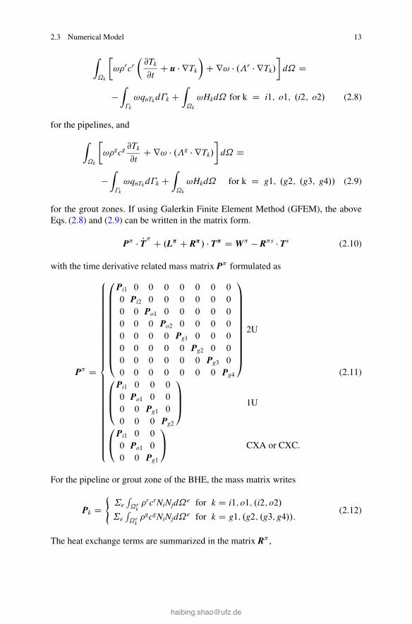
for the grout zones. If using Galerkin Finite Element Method (GFEM), the aboveEqs. (2.8) and (2.9) can be written in the matrix form.
P� � PT� C .L� C R�/ � T� D W� � R�s � Ts (2.10)
with the time derivative related mass matrix P� formulated as
P� D
8ˆˆˆˆˆˆˆˆˆ<
ˆˆˆˆˆˆˆˆˆ:
0
BBBBBBBBBBB@
Pi1 0 0 0 0 0 0 0
0 Pi2 0 0 0 0 0 0
0 0 Po1 0 0 0 0 0
0 0 0 Po2 0 0 0 0
0 0 0 0 Pg1 0 0 0
0 0 0 0 0 Pg2 0 0
0 0 0 0 0 0 Pg3 0
0 0 0 0 0 0 0 Pg4
1
CCCCCCCCCCCA
2U
0
BB@
Pi1 0 0 0
0 Po1 0 0
0 0 Pg1 0
0 0 0 Pg2
1
CCA 1U
0
@Pi1 0 0
0 Po1 0
0 0 Pg1
1
A CXA or CXC.
(2.11)
For the pipeline or grout zone of the BHE, the mass matrix writes
Pk D(˙eR˝e
k�rcrNiNjd˝e for k D i1; o1; .i2; o2/
˙eR˝e
k�gcgNiNjd˝e for k D g1; .g2; .g3; g4//:
(2.12)
The heat exchange terms are summarized in the matrix R� ,

14 2 Theory: Governing Equations and Model Implementations
R�
D
8 ˆ ˆ ˆ ˆ ˆ ˆ ˆ ˆ ˆ ˆ ˆ < ˆ ˆ ˆ ˆ ˆ ˆ ˆ ˆ ˆ ˆ ˆ ˆ :
0 B B B B B B B B B B B @
Ri1
CR
io0
�Rio
0�R
i10
00
0R
i20
00
�Ri2
00
�Rio
0R
ioC
Ro1
00
0�R
o10
00
0R
o20
00
�Ro2
�Ri1
00
0R
i1C2R
g1C
Rg2
CR
s�R
g2�R
g1�R
g1
0�R
i20
0�R
g2R
i2C2R
g1C
Rg2
CR
s�R
g1�R
g1
00
�Ro1
0�R
g1�R
g1R
o1C2R
g1C
Rg2
CR
s0
00
0�R
o2�R
g1�R
g1�R
g2R
o2C2R
g1C
Rg2
CR
s
1 C C C C C C C C C C C A
2U
0 B B @
Ri1
CR
io�R
io�R
i10
�Rio
Ro1
CR
io0
�Ro1
�Ri1
0R
i1C
Rg1
�Rg1
0�R
o1�R
g1R
o1C
Rg1
1 C C A1U
0 @R
i1C
Rio
�Rio
�Ri1
�Rio
Rio
0
�Ri1
0R
i1
1 AC
XA
0 @R
io�R
io0
�Rio
Rio
CR
o1�R
o1
0�R
o1R
o1
1 AC
XA
(2.1
3)

2.3 Numerical Model 15
L� D
8ˆˆˆˆˆˆˆˆˆ<
ˆˆˆˆˆˆˆˆˆ:
0
BBBBBBBBBBB@
Li1 0 0 0 0 0 0 0
0 Li2 0 0 0 0 0 0
0 0 Lo1 0 0 0 0 0
0 0 0 Lo2 0 0 0 0
0 0 0 0 Lig 0 0 0
0 0 0 0 0 Lig 0 0
0 0 0 0 0 0 Log 0
0 0 0 0 0 0 0 Log
1
CCCCCCCCCCCA
2U
0
BB@
Li1 0 0 0
0 Lo1 0 0
0 0 Lg1 0
0 0 0 Lg2
1
CCA 1U
0
@Li1 0 0
0 Lo1 0
0 0 Lg1
1
A CXA or CXC
(2.14)
For the pipeline part, the transport operator L is composed of both advection anddispersion terms,
Lk D ˙eR˝e
k
�Ni�
rcrrNj C rNi � .� � rNj/�
d˝e for k D i1; o1; .i2; o2/:(2.15)
While for the grout zones, only the heat dissipation terms contribute
Lig D Log D ˙eR˝e
krNi � .�g � rNj/d˝e for k D .g1; g2; g3; g4/: (2.16)
For the source and sink terms,
Wk D ˙eR˝e
kNiHkd˝e for 8k: (2.17)
For the heat exchange terms R�s and Rs� ,
Rs� D R�sT D8<
:
.0 0 0 0 �Rs �Rs �Rs �Rs/ 2U
.0 0 �Rs �Rs/ 1U
.0 0 �Rs/ CXA or CXC(2.18)
2.3.3 Assembly of the Global Equation System
In order to simulate the heat transfer between BHEs and the surrounding soil, thegoverning equations for the pipeline and grout zones must be assemble into a global

16 2 Theory: Governing Equations and Model Implementations
matrix system together with the linearized heat transport equation of the soil. Whenthe Eq. (2.10) is combined with the matrix form of Eq. (2.3), the global matrixsystem writes as
�Ps 0
0 P�
�� PTs
PT�!
C�
Ls � R� Rs�
R�s T�
���
Ts
T�
�D�
Ws
W�
�: (2.19)
When Euler time discretization is applied on the above equation, the fullylinearized global matrix system looks like
�As Rs�
Rs� A�
���
Ts
T�
�
nC1D�
Bs
B�
�
nC1;n; (2.20)
where n and n C 1 represents the previous and current time step. If a correctorrecurrence scheme is applied, then the left-hand-side matrix and right-hand-sidevectors writes as
As D 1
tnPs C .Ls � R�/
Bs D�1
tnPs � .1 � / .Ls � R�/
�� Ts
n C WsnC1 C Ws
n.1 � /
A� D 1
tnP� C L�
B� D�1
tnP� � .1 � /L�
�� T�n C W�
nC1 C W�n .1 � / (2.21)
2.3.4 Picard Iterations and Time Stepping Schemes
After the A matrices and B vectors have been assembled, the OpenGeoSys softwareemploys a linear solver to calculate the temperatures T for the new time step,based on the previous time step value. Notice that, the heat exchange coefficientsRs� and R�s will be multiplied with the temperature values, and producing theheat exchange flux between the soil and the BHE domain. This term is linearlydependent on the temperature difference. However, when a new set of temperaturevalues are produced, the heat flux changes respectively. Therefore, a Picard iterationscheme has to be employed by the OpenGeoSys software, to solve for a set ofconverged temperature values. The following log message from a typical simulationdemonstrates the Picard iteration behavior.

2.3 Numerical Model 17
Listing 2.2 Log File of A Simulation Run
================================================->Process 1: HEAT_TRANSPORT_BHE================================================PCS non-linear iteration: 0/2Assembling equation system...Calling linear solver...SpBICGSTAB iteration: 2/1000-->End of PICARD iteration: 0/2PCS error: 0.00110317->Euclidian norm of unknowns: 0.00596578PCS non-linear iteration: 1/2Assembling equation system...Calling linear solver...SpBICGSTAB iteration: 2/1000-->End of PICARD iteration: 1/2PCS error: 1.37569e-006->Euclidian norm of unknowns: 1.82299e-005This step is accepted.Data output: Polyline profile - BHE_1#############################################################
As can be found in the log file, one iteration of the HEAT_TRANSPORT_BHEprocess is needed. In this example, the tolerance of Picard iteration is set to 1:0 �10�4, and the simulation will normally converge after one iteration.
In the work of Diersch et al. (2011a); Diersch (2014), they suggested to inversethe matrix system for BHE domain separately, then integrate its influence into thesoil domain by a Schur complement operation. Such procedures is reasonable asthe BHE domain is typically small (degree of freedom number in the order ofthousands by thousands). However, non-linearity of the governing equations cannotbe eliminated without an iteration step. Their test run also shows that at least oneiteration is necessary to obtain the accurate temperature values. Considering onlylittle effort is added to the linear solver, we choose to directly iterate the linearizedmatrix system of Eq. (2.21). Our simulation shows that convergence can be achieveafter one Picard iteration in nearly all simulations.
Normally at the beginning of the simulation, when refrigerant starts flowing inthe pipeline, the temperature change in the grout and soil is relatively large. Thismakes the model very difficult to converge, i.e. more than dozens of Picard iterationsare required. It is then suggested to specify a small time step size in terms ofminutes for the beginning stage of the simulation. Once the flow and heat transportis stabilized, a larger time step size can then be taken by the model.

Chapter 3OGS Project: Simulating Heat Transport Modelwith BHEs
3.1 Download and Compile the Source Code
Since OpenGeoSys is an open-source project, users can download the source codefrom the following website and build the binary executable file by themselves.
https://github.com/ufz/ogs5For different platforms, i.e. Windows, Mac or Linux, the general procedure
of building an OGS executable and running a model simulation would be verysimilar. Here in this chapter, such process will be demonstrated based on a Windowsoperation system. It will be shown step by step, how to build the source code andconstruct a simple model with one borehole heat exchanger in the middle of themodel domain.
3.1.1 Download the Source Code
Assuming the Git command line interface has already been installed on the system,the OGS source code can be obtained by typing in the command line prompt thefollowing content.
Listing 3.1 Downloading the source code with Git
C:\haibing_working\ogs>git clone https://github.com/ufz/ogs5.git
Or, if one prefers a graphical interface, it is recommend to use SourceTree onthe Windows platform. After a fresh installation of the software SourceTree, thefollowing interface will appear (Fig. 3.1). By clicking the button Clone/New in theupper-left corner, one will be asked to give the location of repository. You may usethe Github link provided above, or first fork from the above repository and clone
© The Author(s) 2016H. Shao et al., Geoenergy Modeling II, SpringerBriefs in Energy,DOI 10.1007/978-3-319-45057-5_3
19

20 3 OGS Project: Simulating Heat Transport Model with BHEs
Fig. 3.1 SourceTree window as in the initial stage
Fig. 3.2 SourceTree dialog asking for the location of the repository
from your own repository on Github (Fig. 3.2). After the code has been successfullycloned to a local drive, one can see all the history of code development in SourceTreeas shown in Fig. 3.3.

3.1 Download and Compile the Source Code 21
Fig. 3.3 SourceTree window with detailed history of a repository
3.1.2 Using CMake to Configure the Building Project
Before the compilation of the source code, the software CMake needs to beemployed to generate the configuration and makefiles which are specific to thebuilding environment. Here the CMake version 2.8.12.2 is employed for demon-stration. In Fig. 3.4, CMake GUI was freshly started. First, one needs to definetwo paths in the CMake GUI. The first one is the folder where the source codeof OGS is located. The second path refers to the folder where the makefiles willbe generated. After clicking on the “Configure” button, CMake will ask severalquestions, depending on different types of operating system and the compilingtools. In this example, the “Visual Studio 2013 x86” option was chosen. Once theconfiguration has finished, the build options will be shown in the CMake GUI. Tobuild the OpenGeoSys code with BHE features, one only needs to choose the optionOGS_FEM. By clicking on the “Generate” button, CMake will prepare all makefilesin the build folder (Fig. 3.5).

22 3 OGS Project: Simulating Heat Transport Model with BHEs
Fig. 3.4 CMake interface of configuring the build information
3.1.3 Compiling the Code
As the author is mainly developing the code with Microsoft Visual Studio, the build-ing process will be demonstrated with the same software. Provided the configurationwas accomplished by CMake successfully in the previous step, there will be a filenamed with “OGS.sln” in the build folder. By opening this Visual Studio solution

3.1 Download and Compile the Source Code 23
Fig. 3.5 CMake interface showing different building options
file, the source code will be loaded into the development environment along withall the building configurations (Fig. 3.6). To build the source code, just choose fromthe menu “BUILD”, and then click on the first option “Build Solution”. It takes acouple of minutes to run the full building process for the first time. After the buildingis completed, an executable file “ogs.exe” can be found under the “bin” folder andthen “Debug” or “Release” folder, depending on which building mode has beenadopted.

24 3 OGS Project: Simulating Heat Transport Model with BHEs
Fig. 3.6 Visual Studio interface after opening the OpenGeoSys solution file
3.2 Define Heat Transport Process with BHEs
In the last section, the OGS code was successfully compiled and an ogs.exeexecutable file has been built. In this section, a modelling project will be establishedto simulate the heat transport process with borehole heat exchangers.
3.2.1 Process Definition
Originally, the heat transport simulation in an OpenGeoSys project is performed bydefining the process as HEAT_TRANSPORT. To include the interaction with BHEs,a new process has been introduced and named as “HEAT_TRANSPORT_BHE”. Themodel input files bear the name “project_name.ext_name”. The “project_name”is a unique string defined by the user to identify a project. The “ext_name” arepre-defined extensions which refers to a particular type of input configuration. Inthe following, a PCS file is first introduced, with one GROUNDWATER_FLOW andone HEAT_TRANSPORT_BHE process defined in it. If the project is named as“bhe_test”, then the PCS file should be named as “bhe_test.pcs”. Its content isshown in the following text box.

3.3 Geometry of BHEs 25
Listing 3.2 PCS File Definition including Interaction with Borehole Heat Exchangers
#PROCESS$PCS_TYPE
GROUNDWATER_FLOW$DEACTIVATED_SUBDOMAIN
11
#PROCESS$PCS_TYPE
HEAT_TRANSPORT_BHE$PRIMARY_VARIABLE
TEMPERATURE_SOIL#STOP
3.2.2 Deactivated Sub-domains
In the above PCS file, some readers might have already noticed that there are twonumbers given under the key word $DEACTIVATED_SUBDOMAIN. The firstnumber “1” on line #7 means there is one sub-domain deactivated for theGROUNDWATER_FLOW process, and the second number “1” on line #8 identifies theindex of this deactivated domain. So why does the sub-domain “1” need to be turnedoff? This is because the sub-domain “0” in this project is referring to the soil domain,while the sub-domain “1” is the borehole heat exchanger compartment. Since theBHE is grouted and impermeable, it is not necessary to calculate groundwater flowthrough a BHE. Therefore its representative sub-domain is deactivated.
3.2.3 Primary Variables
In Sects. 2.1 and 2.2, it has been introduced that there are multiple primary variablesapplied in the BHE simulation. In the soil sub-domain primary variable is the soiltemperature, while on the BHE they are the temperatures of inlet outlet pipes and thesurrounding grout zones. The key words used for these processes, are summarizedin Table 3.1. In Sect. 3.8, when the output is specified, these key words will be used.
3.3 Geometry of BHEs
Listing 3.3 Geometry Definition in the GLI File of an OpenGeoSys Project
#POINTS0 0.0 0.0 18.32 $NAME POINT01 1.8 0.0 18.32 $NAME POINT12 1.8 1.8 18.32 $NAME POINT2

26 3 OGS Project: Simulating Heat Transport Model with BHEs
Table 3.1 Key words used in OGS BHE project for different primary variables
Symbols Key words Meaning
Ts TEMPERATURE_SOIL Soil temperature
Ti1 TEMPERATURE_IN_1 Inflow temperature (1U, CXC, CXA)
Ti2 TEMPERATURE_IN_2 Inflow temperature (2U)
To1 TEMPERATURE_OUT_1 Outflow temperature (1U, CXC, CXA)
To2 TEMPERATURE_OUT_2 Outflow temperature (2U)
Tg1 TEMPERATURE_G_1 Temperature of grout zone 1
Tg2 TEMPERATURE_G_2 Temperature of grout zone 2
Tg3 TEMPERATURE_G_3 Temperature of grout zone 3
Tg4 TEMPERATURE_G_4 Temperature of grout zone 4
3 0.0 1.8 18.32 $NAME POINT34 0.9 0.9 18.32 $NAME POINT45 0.0 0.0 0.0 $NAME POINT56 1.8 0.0 0.0 $NAME POINT67 1.8 1.8 0.0 $NAME POINT78 0.0 1.8 0.0 $NAME POINT89 0.9 0.9 0.0 $NAME POINT910 1.14 0.9 18.32 $NAME POINT1011 1.14 0.9 0.0 $NAME POINT1112 1.34 0.9 18.32 $NAME POINT1213 1.34 0.9 0.0 $NAME POINT1314 1.55 0.9 18.32 $NAME POINT1415 1.55 0.9 0.0 $NAME POINT1516 1.75 0.9 18.32 $NAME POINT1617 1.75 0.9 0.0 $NAME POINT17#POLYLINE$NAMEBHE_1$POINTS49#STOP
As shown in the GLI file above, “BHE_1” is referring to a polyline starting frompoint #4 and ending until point #9. To define different BHEs, each BHE in the modelhas to be given a different polyline in the geometry definition. The geometry nameswill be used afterwards in the MMP and OUT file as a reference to differentiatethe BHEs.
3.4 Mesh of BHEs
In Sect. 2.3.1, it has been already introduced that the BHEs are treated in the OGSmodel as a second domain. Generally, the soil matrix is meshed with 3D prismelements. In comparison to standard mesh file, the location of all mesh nodesremains the same, while additional 1D elements are added at the end of the elementsection, to represent the BHEs.
3.5 Parameters of BHEs 27
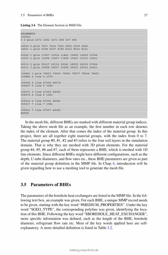
Listing 3.4 The Element Section in MSH File
$ELEMENTS1550620 0 pris 1673 1582 1671 598 507 596...14650 0 pris 7627 7614 7541 6552 6539 646614651 1 pris 9198 9107 9196 8123 8032 8121...23022 1 pris 11927 11914 11841 10852 10839 1076623023 2 pris 13498 13407 13496 12423 12332 12421...56510 2 pris 29127 29114 29041 28052 28039 2796656511 3 pris 30698 30607 30696 29623 29532 29621...154881 3 pris 79652 79639 79566 78577 78564 78491154882 4 line 4 1079...154926 4 line 47304 48379154927 5 line 5 1080...154971 5 line 47305 48380154972 6 line 6 1081...155016 6 line 47306 48381155017 7 line 7 1082...155061 7 line 47307 48382#STOP
In the mesh file, different BHEs are marked with different material group indices.Taking the above mesh file as an example, the first number in each row denotesthe index of the element. After that comes the index of the material group. In thisproject, there are all together eight material groups, with the index from 0 to 7.The material group #0, #1, #2 and #3 refers to the four soil layers in the simulationdomain. That is why they are meshed with 3D prism elements. For the materialgroup #4, #5, #6 and #7, each of them represents a BHE, which is meshed with 1Dline elements. Since different BHEs might have different configurations, such as thedepth, U-tube diameters, and flow rates etc., these BHE parameters are given as partof the material group definition in the MMP file. In Chap. 4, introduction will begiven regarding how to use a meshing tool to generate the mesh file.
3.5 Parameters of BHEs
The parameters of the borehole heat exchangers are listed in the MMP file. In the fol-lowing text box, an example was given. For each BHE, a unique MMP record needsto be given, starting with the key word “#MEDIUM_PROPERTIES”. Under the keyword “$GEO_TYPE”, the corresponding polyline was given, identifying the loca-tion of this BHE. Following the key word “$BOREHOLE_HEAT_EXCHANGER”,more specific information was defined, such as the length of the BHE, boreholediameter, refrigerant flow rate etc. Most of the key words applied here are self-explanatory. A more detailed definition is listed in Table 3.2.

28 3 OGS Project: Simulating Heat Transport Model with BHEsTa
ble
3.2
Para
met
ers
ofB
HE
confi
gura
tion
avai
labl
ein
the
MM
Pfil
e
Def
ault
valu
eR
emar
ksK
eyw
ords
Val
ueto
fill
Uni
t
BHE_TYPE
BHE_TYPE_1U
BHE_TYPE_2U
BHE_TYPE_CXA
BHE_TYPE_CXC
–Sp
ecif
yth
ety
peof
BH
E
BHE_BOUNDARY_TYPE
FIXED_INFLOW_TEMP
FIXED_INFLOW_TEMP_CURVE
POWER_IN_WATT
POWER_IN_WATT_CURVE_FIXED_DT
POWER_IN_WATT_CURVE_FIXED_FLOW_RATE
FIXED_TEMP_DIFF
–D
iffe
rent
boun
dary
cond
ition
sfo
rth
eB
HE
BHE_POWER_IN_WATT_VALUE
Dou
ble
num
ber
WA
fixed
pow
erva
lue
Posi
tive
mea
nshe
atin
gth
eB
HE
,N
egat
ive
mea
nsco
olin
g
BHE_POWER_IN_WATT_CURVE_IDX
Inte
ger
num
ber
–In
dex
ofcu
rve
inth
eR
FDfil
e
BHE_DELTA_T_VALUE
Dou
ble
num
ber
KO
nly
whe
nth
ebo
unda
ryty
peFI
XE
D_T
EM
P_D
IFF
isch
osen
BHE_SWITCH_OFF_THRESHOLD
Dou
ble
num
ber
K
BHE_LENGTH
Dou
ble
num
ber
mL
engt
hof
the
BH
E
BHE_DIAMETER
Dou
ble
num
ber
mD
iam
eter
ofth
ebo
reho
le
BHE_REFRIGERANT_FLOW_RATE
Dou
ble
num
ber
m3=s
Flow
rate
ofci
rcul
atin
gre
frig
eran
tins
ide
the
pipe
line
ofth
eB
HE
BHE_INNER_RADIUS_PIPE
Dou
ble
num
ber
mIn
ner
radi
usof
the
pipe
BHE_OUTER_RADIUS_PIPE
Dou
ble
num
ber
mO
uter
radi
usof
the
pipe
BHE_PIPE_IN_WALL_THICKNESS
Dou
ble
num
ber
mIn
letp
ipe
wal
lthi
ckne
ss
BHE_PIPE_OUT_WALL_THICKNESS
Dou
ble
num
ber
mO
utle
tpip
ew
allt
hick
ness
BHE_FLUID_TYPE
Inte
ger
num
ber
mIn
dex
offlu
idde
fined
inth
eM
FPfil
e
3.5 Parameters of BHEs 29
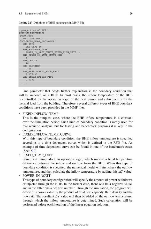
Listing 3.5 Definition of BHE parameters in MMP File
; properties of BHE 1#MEDIUM_PROPERTIES$GEO_TYPE
POLYLINE BHE_1$BOREHOLE_HEAT_EXCHANGER
BHE_TYPEBHE_TYPE_1U
BHE_BOUNDARY_TYPEPOWER_IN_WATT_CURVE_FIXED_FLOW_RATE ;
BHE_POWER_IN_WATT_CURVE_IDX1
BHE_LENGTH46
BHE_DIAMETER0.15
BHE_REFRIGERANT_FLOW_RATE9.17E-05
BHE_INNER_RADIUS_PIPE0.0131
......
One parameter that needs further explanation is the boundary condition thatwill be imposed on a BHE. In most cases, the inflow temperature of the BHEis controlled by the operation logic of the heat pump, and subsequently by thethermal load from the building. Therefore, several different types of BHE boundaryconditions have been provided in the MMP files.
• FIXED_INFLOW_TEMPThis is the simplest case, where the BHE inflow temperature is a constantover the simulation period. Such kind of boundary condition is rarely used forreal scenario analysis, but for testing and benchmark purposes it is kept in theconfiguration.
• FIXED_INFLOW_TEMP_CURVEWith this type of boundary condition, the BHE inflow temperature is specifiedaccording to a time dependent curve, which is defined in the RFD file. Anexample of time dependent curve can be found in one of the benchmark cases(Sect. 5.2).
• FIXED_TEMP_DIFFSome heat pump adopt an operation logic, which impose a fixed temperaturedifference between the inflow and outflow from the BHE. When this type ofboundary condition is specified, the numerical model will first check the outflowtemperature, and then calculate the inflow temperature by adding this T value.
• POWER_IN_WATTThis type of boundary configuration will specify the amount of power withdrawnor injected through the BHE. In the former case, there will be a negative value,and in the latter one a positive number. Through the simulation, the program willdivide this power value by the product of fluid heat capacity, fluid density and theflow rate. The resultant T value will then be added on the outflow temperature,through which the inflow temperature is determined. Such calculation will beperformed before each iteration of the linear equation solution.

30 3 OGS Project: Simulating Heat Transport Model with BHEs
• POWER_IN_WATT_CURVE_FIXED_DTIn this scenario, the BHE thermal load is specified according to a predefinedcurve in the RFD file. Meanwhile, a fixed T values will be maintained, i.e. theflow rate will be dynamically calculated based on the thermal load, the circulatingfluid properties, and the given T value. If the resultant flow rate is below acertain threshold (by default 1:0 � 10�6 m3=s, the program will assume that theheat pump and fluid circulation is switched off.
• POWER_IN_WATT_CURVE_FIXED_FLOW_RATEDifferent from the previous configuration, this type of boundary will maintaina fixed flow rate instead of T . In this case the T value will be dynamicallycalculated using the same relationship, while the flow rate is kept the same.
• BHE_BOUND_BUILDING_POWER_IN_WATT_CURVE_FIXED_DTandBHE_BOUND_BUILDING_POWER_IN_WATT_CURVE_FIXED_FLOW_RATEThe additional feature in these two types of boundary is the inclusion ofheat pump efficiency. Conventionally, this efficiency value is quantified by thecoefficient of performance (COP) Casasso and Sethi (2014)
COP DPQ
W(3.1)
where PQ is the amount of thermal power required by the building, and W isthe electricity consumed by the heat pump. The COP can be determined by thetemperature of circulating fluid at the BHE outlet, and the temperature requiredat the heating end [see Jaszczur and Sliwa (2013) and also Eq. (3.2)]. Althoughthere are other factors influencing the heat pump COP, it is widely assumedthat the COP is linearly dependent on the BHE outflow temperature. The samesimplification can be found in e.g. Kahraman and Çelebi (2009), Casasso andSethi (2014) and Sanner et al. (2003). The COP of a typical heat pump can beapproximated by the following relationship,
COP D a C bTout (3.2)
where the parameters a and b is can be defined in the MMP file.In reality, the thermal load of the BHE PQBHE is not the same as the building
heat demand PQBuilding (see e.g. Casasso and Sethi 2014; Eicker and Vorschulze2009; Speer 2005). To shift the heat from the ground to the building, the heatpump needs about 20–30 % of the energy in the form of electricity. This amountof heat must be subtracted from the thermal load.
PQBHE D PQBuildingCOP � 1
COP(3.3)
This effect will be explicitly considered by these two boundary conditions.With these two configurations, the building thermal load is specified. During the
3.6 Initial Conditions for the BHE 31
model simulation, the COP of the heat pump will be dynamically calculated byOGS, and the amount of BHE thermal load will be updated accordingly.
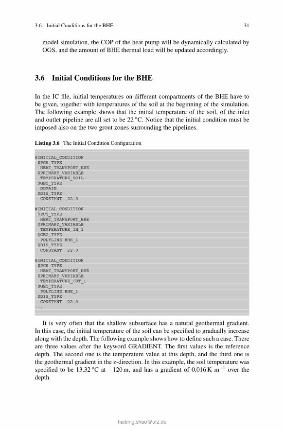
3.6 Initial Conditions for the BHE
In the IC file, initial temperatures on different compartments of the BHE have tobe given, together with temperatures of the soil at the beginning of the simulation.The following example shows that the initial temperature of the soil, of the inletand outlet pipeline are all set to be 22 ıC. Notice that the initial condition must beimposed also on the two grout zones surrounding the pipelines.
Listing 3.6 The Initial Condition Configuration
#INITIAL_CONDITION$PCS_TYPEHEAT_TRANSPORT_BHE
$PRIMARY_VARIABLETEMPERATURE_SOIL
$GEO_TYPEDOMAIN
$DIS_TYPECONSTANT 22.0
#INITIAL_CONDITION$PCS_TYPEHEAT_TRANSPORT_BHE
$PRIMARY_VARIABLETEMPERATURE_IN_1
$GEO_TYPEPOLYLINE BHE_1
$DIS_TYPECONSTANT 22.0
#INITIAL_CONDITION$PCS_TYPEHEAT_TRANSPORT_BHE
$PRIMARY_VARIABLETEMPERATURE_OUT_1
$GEO_TYPEPOLYLINE BHE_1
$DIS_TYPECONSTANT 22.0
...
It is very often that the shallow subsurface has a natural geothermal gradient.In this case, the initial temperature of the soil can be specified to gradually increasealong with the depth. The following example shows how to define such a case. Thereare three values after the keyword GRADIENT. The first values is the referencedepth. The second one is the temperature value at this depth, and the third one isthe geothermal gradient in the z-direction. In this example, the soil temperature wasspecified to be 13.32 ıC at �120m, and has a gradient of 0.016 K m�1 over thedepth.

32 3 OGS Project: Simulating Heat Transport Model with BHEs
Listing 3.7 Initial Condition with Geothermal Gradient
...#INITIAL_CONDITION$PCS_TYPEHEAT_TRANSPORT_BHE
$PRIMARY_VARIABLETEMPERATURE_SOIL
$GEO_TYPEDOMAIN
$DIS_TYPEGRADIENT -120 13.32 0.016
...
3.7 Boundary Conditions for the BHE
In Sect. 3.5, the different types of BHE boundary conditions have already beendiscussed in detail. Besides these configurations, the user still needs to define inthe BC file, where the boundary condition should be applied. The following textbox shows an example. Here two locations have been specified. The first one wasdefined on the starting node of the BHE, namely on POINT4. At this location, theinflow temperature was imposed according to curve #1 defined in the RFD file (seeSect. 5.2 for an example). The second location is on POINT9, which is at the bottomof the BHE. This second location is necessary, because OGS will internally read howhigh the temperature is on the inflow pipe and impose this value on the outflow pipe.Therefore, the value imposed on POINT9 will not have any effect on the simulationresult.
Listing 3.8 Boundary condition configuration in the BC file
...#BOUNDARY_CONDITION$PCS_TYPEHEAT_TRANSPORT_BHE
$PRIMARY_VARIABLETEMPERATURE_IN_1
$GEO_TYPEPOINT POINT4
$DIS_TYPECONSTANT 1.0
$TIM_TYPECURVE 1
#BOUNDARY_CONDITION$PCS_TYPEHEAT_TRANSPORT_BHE
$PRIMARY_VARIABLETEMPERATURE_OUT_1
$GEO_TYPEPOINT POINT9
$DIS_TYPECONSTANT 5.0
...

3.9 Running the OGS Model 33
3.8 Output of Temperatures
In the OUT file, it is configured which of the simulated temperature values aregoing to be recorded by OGS. As shown in the following example, two differentoutput records are specified, each starting with the key word #OUTPUT. In the firstone, the soil temperature over the entire domain is printed out in the PVD format.In the second one, the inlet, outlet temperature of the pipe, the two grout zonessurrounding them, and also the soil temperature along the BHE is plotted in theTECPLOT format. Under the key word TIM_TYPE, the specification “STEPS 10”means that the simulation result will be printed once in every ten time steps. Boththe PVD format and the TECPLOT format output files can be read by a text editor.
Listing 3.9 The Output Configuration
#OUTPUT$PCS_TYPE
HEAT_TRANSPORT_BHE$NOD_VALUES
TEMPERATURE_SOIL$GEO_TYPE
DOMAIN$DAT_TYPE
PVD$TIM_TYPE
STEPS 10#OUTPUT
$PCS_TYPEHEAT_TRANSPORT_BHE
$NOD_VALUESTEMPERATURE_IN_1_BHE_1TEMPERATURE_OUT_1_BHE_1TEMPERATURE_G_1_BHE_1TEMPERATURE_G_2_BHE_1TEMPERATURE_SOIL
$GEO_TYPEPOLYLINE BHE_1
$DAT_TYPETECPLOT
$TIM_TYPESTEPS 10
#STOP
3.9 Running the OGS Model
There are several ways to start the simulation. In general, the OGS simulator can bestarted by calling the executable file ogs.exe. The easiest approach would be to runthe simulation in the same folder where the input files are located. After copying theogs.exe file into the project folder, one can double-click on the executable, then thefollowing windows will appear on the screen (cf. Fig. 3.7). Within this window, onecan enter the project name without the dot and any extensions. As the input files are

34 3 OGS Project: Simulating Heat Transport Model with BHEs
Fig. 3.7 Starting the simulation by calling the executable ogs.exe
Fig. 3.8 Starting the simulation by calling the executable ogs.exe
name as “bhe_test.�”, entering “bhe_test” will be sufficient. After hitting the Enterkey, the simulation will start.
An alternative approach is to have the executable placed at a different location,but supply the executable with the path to the project. As illustrated in Fig. 3.8, nowogs.exe is located under “C:nhaibingnworkingntmp”. After launching ogs.exe, onecan enter the project path “C:nhaibing_workingnogsn bhe_testsnbhe_test” to startthe simulation. A easier way would be, to drag and drop one of the input files intothe OGS command line prompt, and delete the extensions. As the OGS is designedto run on multiple platforms, it can not read in folder or file names with space in

3.10 Visualization of Temperature Evolution 35
it. Please make sure that the path of the input files does not contain any space orspecial characters, otherwise OGS will not be able to find the right location.
While running the simulation, there is quiet a lot of logging information beingprinted on the screen. It includes which time step the simulation is in, how manynonlinear and linear iterations have been conducted, and how big is the numericalresidual when solving the linear system. Such information is very helpful to themodeller, therefore it is recommended to save them in a log file. To do this, onecould create an empty batch file, eg. named as “run_ogs.bat”. Within it, just type inthe following content.
Listing 3.10 The content of the batch file
ogs.exe bhe_test > result.txt
Here the symbol “>” will pipeline the screen output to the file “result.txt”. Byusing this method, the user can open this text file and check the modelling progresswhile the simulation is still running.
3.10 Visualization of Temperature Evolution
As defined in the OUT file, there are two records in the output configuration, one forthe soil temperatures, and the other for the inflow, outflow and grout temperatureson the BHEs (see the introduction in Sect. 3.8).
3.10.1 Visualization of Soil Temperatures
For the soil temperatures, they are recorded in the VTK format, and can be directlyvisualized by the software Paraview. As shown in Fig. 3.9, the result files are nameas “bhe_test_HEAT_TRANSPORT_BHE*.*”. The first part of the file name is thesame as all the input files, while the second part is composed of the process that wassimulated. For each of the *.vtu files, there is a number appending the file name, itreflects which time step this file belongs to. When visualizing the soil temperatures,one could directly load the *.pvd file, making paraview to read in all the printedresult. Alternatively, one can also load a single *.vtu file, which only contains thesoil temperature distribution at this time step.
Figure 3.10 demonstrates how the soil temperature will be influence by theBHE operation. In this example, the sandbox experiment from Beier et al. (2011)was reproduced (see Sect. 5.2 for more details). Since heat is injected through theU-tubes, the temperature at the center of the sandbox will gradually increase alongtime. This is reflected by red color at the center of the domain (Fig. 3.10).

36 3 OGS Project: Simulating Heat Transport Model with BHEs
Fig. 3.9 Result files by a simulated OGS project
3.10.2 Visualization of BHE Temperatures
Different from the soil part, the information regarding temperatures inside theborehole heat exchanger is typically printed in the Tecplot file format. Figure 3.11shows such an example. Here there are altogether six columns listed. From the leftto the right, it is the distance from the top of the BHE, temperatures in the inflowand outflow pipeline, temperatures on the two grout zones, and finally BHE walltemperature. The order of the columns is actually defined in the *.out file. Noticethat the pipeline temperature values at the bottom of the BHE, specifically on line#24 and #46, are kept the same. One can also import the data into a spreadsheet orplotting software, then the temperature distribution on each BHE can be visualizedin a vertical profile.

3.10 Visualization of Temperature Evolution 37
Fig. 3.10 Visualization effect of the simulated soil temperature distribution by the softwareParaview

38 3 OGS Project: Simulating Heat Transport Model with BHEs
Fig. 3.11 Simulated temperature values printed in the Tecplot file format

Chapter 4BHE Meshing Tool
In general, there are various approaches to create mesh files. One could try tocreate the line elements representing BHEs by hand. However, such practice isquiet cumbersome and also very prone to mistakes. To alleviate the user from thisburden, a simple meshing tool has been provided. It can be downloaded from theOGS website.
https://docs.opengeosys.org/books/shallow-geothermal-systemsIn the provided package, a binary executable has been built for the Windows
platform. For users of other platforms, they need to build the meshing tool from theprovided source codes.
This meshing tool is capable of creating a 3D prism mesh of the subsurface witharbitrary number of horizontal layers in different thickness, along with differentmaterial groups and arbitrary number of vertical BHEs. To use the BHE meshingtool, one also need the software GMSH, which is an open-source finite elementmesh generator. Software download and tutorials of GMSH can be found on itsofficial website (www.gmsh.info). It is necessary to place both binaries files, i.e. thebhe_meshing_tool.exe and the gmsh.exe in the same working folder.
The work flow is organized in the following order:
(1) Read in the input file.(2) Create a GMSH geometry file according to specifications defined in the input
file.(3) Call the GMSH to create the 2D surface mesh.(4) Import the mesh created in step (3).(5) Extrude the surface mesh according to layer specifications made in the input
file.(6) Generate BHE elements according to specifications made in the input file.(7) Write the corresponding mesh file into OGS format.(8) Write the corresponding geometry file into OGS format.
© The Author(s) 2016H. Shao et al., Geoenergy Modeling II, SpringerBriefs in Energy,DOI 10.1007/978-3-319-45057-5_4
39

40 4 BHE Meshing Tool
4.1 Requirement on the Mesh
As mentioned in Diersch et al. (2011b), when the BHE is represented by 1Delements, the amount of heat flux between BHE and the surrounding soil is heavilyinfluenced by the size of mesh elements in the vicinity of the BHE node. Toguarantee the accuracy of simulation result, Diersch et al. (2011b) proposed aprocedure to determine the optimal nodal distance, that is influenced by the numberof nodes surrounding the BHE center node, as well as the borehole diameter. Theoptimal distance can be obtained by
D arb; a D e2�# ; # D n tan
�
n; (4.1)
with rb denotes the borehole radius, and n refers to the number of surroundingnodes. is increasing along with the number n. When designing the mesh withthe provided meshing tool, the above criteria has already been considered to ensurethe correct heat flux over the borehole wall, which will influence all inlet, outletand grout temperatures on the BHE nodes. Deviation from Eq. (4.1) will lead toinaccurate solutions. The meshing tool always operates with a number of n D 6
nodes. If a different setup is required, the user may want to modify the source codeof this meshing tool, which is also provided.
4.2 Input File for the Meshing Tool
To run the meshing tool, one can type the following command.
Listing 4.1 Run the meshing tool
>bhe_meshing_tool.exe inputfile
Here the inputfile is an ASCII file containing all configurations for generating thecomplete 3D mesh. If the user wishes a 2D mesh output, one can type
Listing 4.2 Run the meshing tool to generate 2D mesh
>bhe_meshing_tool.exe inputfile -2D
to generate a surface 2D mesh only. This is useful for the inspection of the surfacemesh before it will be extruded. All information required to generate a completemesh including BHEs have to be supplied in the input file. An example is given hereand the key words and parameters are explained.

4.2 Input File for the Meshing Tool 41
Listing 4.3 Input file: example.inp
WIDTH 100LENGTH 200DEPTH 90BOX 50 100 50// BOX -1 -1 -1ELEM_SIZE 5 20LAYER 0 10 1LAYER 1 20 2LAYER 2 10 4BHE 0 -10 100 0 -50 0.063BHE 1 10 100 0 -30 0.063
• WIDTH: Domain width in the x-direction. Note that the model is centred in thex-direction. This means, the domain here would extend from �50 to 50 in the xdirection.
• LENGTH: Domain length in the y-direction. Note that the origin is at the frontboundary. In the example above, the domain would extend from y=0..200
• DEPTH: Domain thickness in the negative z-direction. Note that the surface isalways at z=0. Therefore in the example above, the domain would extend fromz=0..�90. This parameter only affects the creation of the geometry file. The meshwill be extruded according to the definition of layers (see the LAYER keywordbelow).
• BOX: Here, a refinement box can be defined. Parameters arey-coordinate of the box frontlength of the boxwidth of the box
In the example above, the box would extend from x=�25..25 and y=50..150. Ifthe model shall not contain a refinement box, the values have to be replaced by�1.
• ELEM_SIZE: This defines the element size at the boundary of the refinementbox and the outer boundaries. If no refinement box is employed, the first valuewill be overrun.
• LAYER: Specification of each layer with following parameters:material group index valuenumber of elements in this layerthickness of each element in this layer
The thickness of layer is then dependent on the number of elements, as well asthe thickness of each element. Please make sure that the definition of domaindepth, layers and vertical extent of BHEs match with each other.
• BHE: Here, the BHEs are defined with the following parameters:Number of BHE (This number is only referring to the total number of BHEs,
NOT the corresponding material groups. The material groups will be generatedand linked with BHE automatically. )
x-coordinate of BHE centery-coordinate of BHE centerz-coordinate of BHE top endz-coordinate of BHE bottom end

42 4 BHE Meshing Tool
The user has to make sure, that layers boundaries are located properly at the BHEtop and bottom ends. The algorithm in the meshing tool will automatically pickup the nearest mesh nodes in the z-direction, and generate BHE elements withthese mesh nodes.
4.3 Output
After execution of the meshing tool, the following files will be written in the workingfolder.
• example.bhe.msh: This is the OGS mesh file. In order to use it for running asimulation, one would have to rename it by deleting the extension “.bhe” fromthe file name. The content of this mesh file is listed in the following text box, andthe visualized effect of this mesh is illustrated in Figs. 4.1 and 4.2.
Listing 4.4 example.bhe.msh
#FEM_MSH$PCS_TYPENO_PCS$NODES505120 -50 0 01 50 0 02 50 200 03 -50 200 0[..]50510 -4.9577 100.738 -9050511 4.96093 100.753 -90$ELEMENTS973300 0 pris 1092 122 503 2324 1354 17351 0 pris 1091 504 121 2323 1736 13532 0 pris 1178 387 233 2410 1619 1465[..]24318 0 pris 11502 11834 11973 12734 13066 1320524319 0 pris 11503 11971 11832 12735 13203 1306424320 1 pris 13412 12442 12823 14644 13674 1405524321 1 pris 13411 12824 12441 14643 14056 13673[..]72958 1 pris 36142 36474 36613 37374 37706 3784572959 1 pris 36143 36611 36472 37375 37843 3770472960 2 pris 38052 37082 37463 39284 38314 3869572961 2 pris 38051 37464 37081 39283 38696 3831372962 2 pris 38138 37347 37193 39370 38579 38425[..]97278 2 pris 48462 48794 48933 49694 50026 5016597279 2 pris 48463 48931 48792 49695 50163 5002497280 3 line 8 1240 97281 3 line 1240 2472[..]97308 3 line 34504 3573697309 3 line 35736 3696897310 4 line 15 124797311 4 line 1247 2479[..]97329 4 line 23423 24655#STOP

4.3 Output 43
Fig. 4.1 3D mesh
Fig. 4.2 3D mesh, line elements inside
• example.geo: This is the geometry input file for GMSH.• example.gli: This is the OGS geometry file (illustrated in Fig. 4.3). The six sur-
faces of the cube are named as top, bottom, left, right, inflow,outflow. Important definitions for the BHEs are the top and bottom points aswell as the BHE polylines, which are named in a systematic manner.

44 4 BHE Meshing Tool
Fig. 4.3 Geometry
Listing 4.5 example.gli
#POINTS0 -50 0 01 50 0 0[..]8 -10 100 0 $NAME BHE0_top9 -10 100 -50 $NAME BHE0_bottom10 10 100 0 $NAME BHE1_top11 10 100 -30 $NAME BHE1_bottom[..]#POLYLINE$NAMEply_BHE0$POINTS89#POLYLINE$NAMEply_BHE1$POINTS1011[..]#STOP
• example.msh: This is the 2D surface mesh generated by GMSH (illustrated inFig. 4.4). Please notice that this 2D mesh is only generated intermediately andit is NOT for OGS model simulation. For the OGS input, the 3D mesh fileexample.bhe.msh should be used.


Chapter 5Benchmarks
In order to verify both the heat transport process that is induced by the operationof BHEs, two benchmark comparisons have been carried out. In the first case,the result from analytical Infinite Line Source Model has been used as a standard(Sect. 5.1). In the second case, the numerically simulated outflow temperatures havebeen compared to observations from an indoor sandbox experiment (Sect. 5.2).
5.1 Borehole Heat Exchangers: Comparison to Line SourceModel
Here in this benchmark, the soil temperature evolution induced by a BHE is obtainedfrom three different configurations. They are:
• Using the infinite line source (ILS) analytical solution, assuming heat is evenlyextracted over the length of a BHE.
• By simulating the HEAT_TRANSPORT process using OpenGeoSys, also assum-ing heat is evenly extracted by the BHE.
• By simulating the newly developed HEAT_TRANSPORT_BHE process inOpenGeoSys. Although the same thermal load is imposed on the BHE, this newprocess allows the dynamic development of pipeline and grout temperatures aswell.
All three configurations have been established with the same geometry, initialconditions, and material parameters etc., which are listed in Table 5.1. It isknown that the analytical line source model will produce inaccurate results of soiltemperature in the immediate vicinity of the BHE. Nevertheless, the results shouldconverge at a couple of meters away from the BHE. The result comparison will bepresented in Sect. 5.1.4.
© The Author(s) 2016H. Shao et al., Geoenergy Modeling II, SpringerBriefs in Energy,DOI 10.1007/978-3-319-45057-5_5
47

48 5 Benchmarks
Table 5.1 Parameters used in the line source model comparison
Parameter Symbol Value Unit
Specific thermal load on the BHE qb �5:68 W m�1
Length of the BHE LBHE 46 m
Thermal load on the BHE Q �261:68 W
Soil thermal conductivity �soil 1:34 W m�1 K�1
Heat capacity of soil .�cp/soil 2� 106 J m�3 K�1
BHE type 1U
Diameter of the BHE DBHE 15 cm
Diameter of the pipeline dpipe 3:98 cm
Wall thickness of the pipeline bpipe 0:36 cm
Distance between the pipelines w 6:3 cm
Thermal conductivity of pipeline wall �pipe 0:39 W m�1 K�1
Thermal conductivity of the grout �grout 0:73 W m�1 K�1
Heat capacity of the grout .�cp/grout 3:8� 106 J m�3 K�1
Thermal conductivity of the refrigerant �refrigerant 0:477 W m�1 K�1
Heat capacity of the refrigerant .�cp/refrigerant 3:838 � 106 J m�3 K�1
Viscosity of the refrigerant �refrigerant 3:04 � 10�3 kg m�1 s�1
Flow rate of the refrigerant Qrefrigerant 15:087 m3 d�1
5.1.1 ILS Analytical Solution
When using the infinite line source (ILS) solution (Stauffer et al. 2014), soiltemperatures are expressed in difference values in comparison to the undisturbedinitial temperature T0 at a radial distance rb. And this difference is given by
T � T0 D qb
4��E1 r2b4˛t
�(5.1)
with qb referring to the heat flow rate per length of BHE, thermal diffusivity ˛ D ��cp
and the exponential integral function E1.
5.1.2 Numerical Line Source Model
In the numerical line source model, a domain has been constructed, with a singleBHE located in the middle of it. Here the numerical process HEAT_TRANSPORThas been simulated. A constant source term of qb was imposed on a polylinerepresenting the BHE (cf. Fig. 5.1). Here, a constant heat source (a Neumann-typeof boundary condition) of �5:68W=m is applied on the polyline “BHE_1”. Thefollowing text box shows how the ST file was defined.
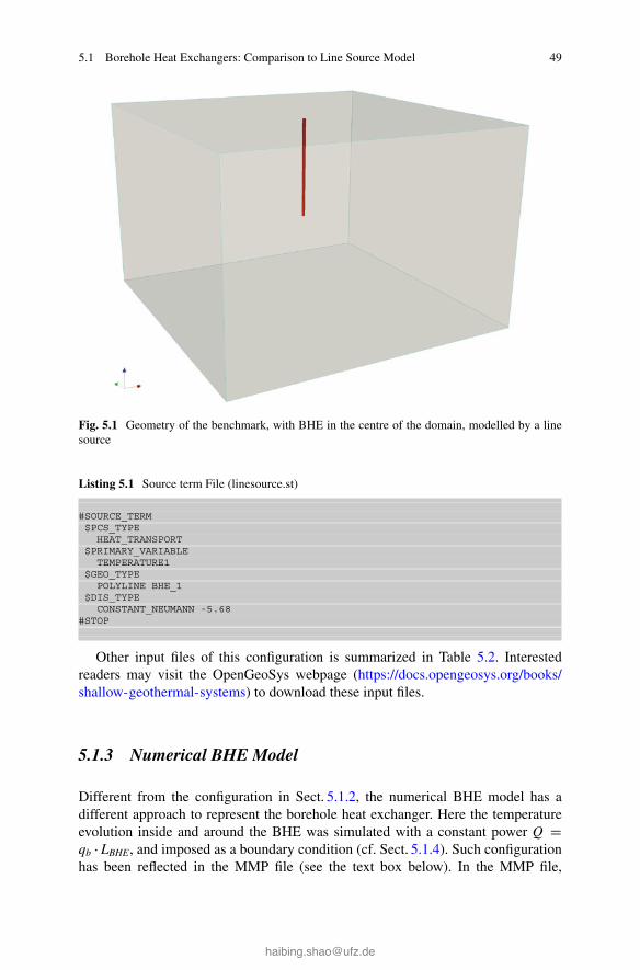
5.1 Borehole Heat Exchangers: Comparison to Line Source Model 49
Fig. 5.1 Geometry of the benchmark, with BHE in the centre of the domain, modelled by a linesource
Listing 5.1 Source term File (linesource.st)
#SOURCE_TERM$PCS_TYPE
HEAT_TRANSPORT$PRIMARY_VARIABLE
TEMPERATURE1$GEO_TYPE
POLYLINE BHE_1$DIS_TYPE
CONSTANT_NEUMANN -5.68#STOP
Other input files of this configuration is summarized in Table 5.2. Interestedreaders may visit the OpenGeoSys webpage (https://docs.opengeosys.org/books/shallow-geothermal-systems) to download these input files.
5.1.3 Numerical BHE Model
Different from the configuration in Sect. 5.1.2, the numerical BHE model has adifferent approach to represent the borehole heat exchanger. Here the temperatureevolution inside and around the BHE was simulated with a constant power Q Dqb � LBHE, and imposed as a boundary condition (cf. Sect. 5.1.4). Such configurationhas been reflected in the MMP file (see the text box below). In the MMP file,

50 5 Benchmarks
Table 5.2 OGS input filesfor the Numerical LineSource model
Object File Explanation
GEO linesource.gli System geometry
MSH linesource.msh Finite element mesh
PCS linesource.pcs Process definition
NUM linesource.num Numerical properties
TIM linesource.tim Time discretization
IC linesource.ic Initial conditions
BC linesource.bc Boundary conditions
ST linesource.st Source/sink terms
MSP linesource.msp Solid properties
MMP linesource.mmp Medium properties
OUT linesource.out Output configuration
the material group #0 refers to the soil part. Since no groundwater flow processis considered, all values are zero. Material group #1 represents the BHE. Here, allrelevant parameters for the BHE model are entered, according to the values given inTable 5.1. What is special here is that, the boundary condition type for the BHEs isset to be “POWER_IN_WATT”. This means a fixed thermal load will be imposedon the BHE. The inflow refrigerant temperature will be automatically adjusted tosatisfy this thermal load.
Listing 5.2 Medium Properties File (BHE.mmp)
#MEDIUM_PROPERTIES$GEO_TYPEDOMAIN
$GEOMETRY_DIMENSION3
$GEOMETRY_AREA1
$POROSITY1 0.0
$PERMEABILITY_TENSORISOTROPIC 0.0
$HEAT_DISPERSION1 0.0 0.0
#MEDIUM_PROPERTIES$GEO_TYPEPOLYLINE BHE_1
$GEOMETRY_DIMENSION1
$GEOMETRY_AREA1
$BOREHOLE_HEAT_EXCHANGERBHE_TYPE
BHE_TYPE_1UBHE_BOUNDARY_TYPE
POWER_IN_WATTBHE_POWER_IN_WATT_VALUE
-261.28BHE_LENGTH
46BHE_DIAMETER
0.15

5.1 Borehole Heat Exchangers: Comparison to Line Source Model 51
BHE_REFRIGERANT_FLOW_RATE1.746E-04
BHE_INNER_RADIUS_PIPE0.0163
BHE_OUTER_RADIUS_PIPE0.0199
BHE_PIPE_IN_WALL_THICKNESS0.0036
BHE_PIPE_OUT_WALL_THICKNESS0.0036
BHE_FLUID_TYPE0
BHE_FLUID_LONGITUDIAL_DISPERSION_LENGTH0.0
BHE_GROUT_DENSITY2190.0
BHE_GROUT_POROSITY0.0
BHE_GROUT_HEAT_CAPACITY1735.16
BHE_THERMAL_CONDUCTIVITY_PIPE_WALL0.39
BHE_THERMAL_CONDUCTIVITY_GROUT0.73
BHE_PIPE_DISTANCE0.063
#STOP
In the BC file, two records have to be made for the inlet temperature at the top ofthe BHE and the outlet temperature at the bottom of the BHE. These two boundaryconditions are required by OGS in order to locate top and bottom nodes of the BHE.Since a power boundary conditions on the BHE has already been defined, the valuesentered here can be arbitrary, because they will not be considered throughout thesimulation.
Listing 5.3 Boundary condition File (BHE.bc)
#BOUNDARY_CONDITION$PCS_TYPE
HEAT_TRANSPORT_BHE$PRIMARY_VARIABLE
TEMPERATURE_IN_1$GEO_TYPE
POINT BHE1_TOP$DIS_TYPE
CONSTANT 1.0#BOUNDARY_CONDITION$PCS_TYPE
HEAT_TRANSPORT_BHE$PRIMARY_VARIABLE
TEMPERATURE_OUT_1$GEO_TYPE
POINT BHE1_BOTTOM$DIS_TYPE
CONSTANT 1.0#STOP

52 5 Benchmarks
Fig. 5.2 Observation points in line source model
5.1.4 Results
Soil temperatures were observed at two locations, one at a distance of r1 D 6:0manother at r2 D 1:6m (c.f. Fig. 5.2). Good agreement has been reached betweenthe analytical line source model solution and the numerical results. The comparisonof temperature profiles can be found in Figs. 5.3 and 5.4. From these two figures,it can be concluded that the two numerical model configurations produce correctresult regarding the soil temperature evolution. This comparison also suggests thatthe temperature difference along the BHE length is relatively small. It is safe toassume that the thermal load will be evenly distributed along the entire BHE length,and it will not generate observable changes on the soil temperatures.
5.2 Borehole Heat Exchangers: Comparison to SandboxExperiment
In this benchmark, the Borehole Heat Exchanger (BHE) feature in the OGS softwareis validated against experimental results obtained by Beier et al. (2011). In theirexperiment, a Thermal Response Test (TRT) was performed under controlledconditions on a single U-tube borehole heat exchanger placed inside a sand box.Inlet and outlet fluid temperatures were monitored together with temperatures at theborehole wall and at different locations in the sand box.

5.2 Borehole Heat Exchangers: Comparison to Sandbox Experiment 53
t/[days]
0 100 200 300
T/[°
C]
9.6
9.7
9.8
9.9
10.0
analytical ILS modelnumerical line source modelBHE model
Fig. 5.3 Comparison of soil temperature profile at 6.0 m distance
t/[days]
0 100 200 300
T/[°
C]
8.6
8.8
9.0
9.2
9.4
9.6
9.8
10.0
analytical ILS modelnumerical line source modelBHE model
Fig. 5.4 Comparison of soil temperature profile at 1.6 m distance

54 5 Benchmarks
5.2.1 Model Setup
The model was built according to the experimental configurations. The BHE isrepresented by line elements which are embedded in a 3D prism mesh representingthe sandbox (Fig. 5.5). The length of the box is 18m with a square cross sectionof 1.8 m per side. Detailed parameters for the model configuration can be found inTable 5.3.
In Beier’s experiment, there was an aluminium pipe acting as the borehole wall.It cannot be represented by the BHE model itself, therefore the borehole diameterwas taken as the aluminium pipe’s outer diameter of 0:13m in the numerical model.The grout’s thermal conductivity was increased from originally 0:73W m�1 K�1 to0:806W m�1 K�1, in order to include the aluminium pipe’s thermal conductivityand its geometry. The BHE is filled with water. Thermal properties and viscosity ofwater are taken at an average temperature of approx. 36 ıC.
Fig. 5.5 Sandbox model
Table 5.3 Benchmark parameters according to Beier’s sandbox experiment(Beier et al. 2011)
Parameter Symbol Value Unit
Soil thermal conductivity �soil 2.78 W m�1 K�1
Soil heat capacity .�cp/soil 3:2� 106 J m�3 K�1
Diameter of the BHE DBHE 13 cm
Diameter of the pipeline dpipe 2.733 cm
Wall thickness of the pipeline bpipe 0.3035 cm
Distance between pipelines w 5.3 cm
Pipeline wall thermal conductivity �pipe 0.39 W m�1 K�1
Grout thermal conductivity �grout 0.806 W m�1 K�1
Heat capacity of the grout .�cp/grout 3:8� 106 J m�3 K�1

5.2 Borehole Heat Exchangers: Comparison to Sandbox Experiment 55
5.2.2 OGS Input Files
The OGS input files used in this benchmark is very similar as those in Sect. 5.1.Here only the unique parts are highlighted.
5.2.2.1 Initial and Boundary Conditions
Initial conditions for fluid inlet/outlet temperatures and wall temperature weredirectly taken from the measurements at t D 0. For the initial soil temperature, themean value of all sensors placed in the sand was taken. As initial grout temperatures,arithmetic mean between wall and fluid inlet/outlet temperature was taken. Detailedinitial temperatures can be found in Table 5.4.
Listing 5.4 Initial Condition File (Beier.ic)
#INITIAL_CONDITION$PCS_TYPE
HEAT_TRANSPORT_BHE$PRIMARY_VARIABLE
TEMPERATURE_SOIL$GEO_TYPE
DOMAIN$DIS_TYPE
CONSTANT 22.1#INITIAL_CONDITION$PCS_TYPE
HEAT_TRANSPORT_BHE$PRIMARY_VARIABLE
TEMPERATURE_SOIL$GEO_TYPE
POLYLINE BHE_1$DIS_TYPE
CONSTANT 21.95#INITIAL_CONDITION$PCS_TYPE
HEAT_TRANSPORT_BHE$PRIMARY_VARIABLE
TEMPERATURE_IN_1$GEO_TYPE
POLYLINE BHE_1$DIS_TYPE
CONSTANT 22.21
Table 5.4 Initial conditions of sandbox model
Parameter Symbol Value Unit
BHE inlet temperature Tin 22:21 ıC
BHE outlet temperature Tout 21:98 ıC
Grout temperature around inlet pipe Tgrout1 22:08 ıC
Grout temperature around outlet pipe Tgrout2 21:97 ıC
Soil temperature Tsoil 22:10 ıC
BHE wall temperature Twall 21:95 ıC

56 5 Benchmarks
#INITIAL_CONDITION$PCS_TYPE
HEAT_TRANSPORT_BHE$PRIMARY_VARIABLE
TEMPERATURE_OUT_1$GEO_TYPE
POLYLINE BHE_1$DIS_TYPE
CONSTANT 21.98#INITIAL_CONDITION$PCS_TYPE
HEAT_TRANSPORT_BHE$PRIMARY_VARIABLE
TEMPERATURE_G_1$GEO_TYPE
POLYLINE BHE_1$DIS_TYPE
CONSTANT 22.08#INITIAL_CONDITION$PCS_TYPE
HEAT_TRANSPORT_BHE$PRIMARY_VARIABLE
TEMPERATURE_G_2$GEO_TYPE
POLYLINE BHE_1$DIS_TYPE
CONSTANT 21.965#STOP
The boundary conditions are imposed on the BHE as time series of measuredinlet fluid temperature and flow rate as demonstrated in Fig. 5.6. Note that theBHE top boundary condition is different (cf. MMP file), as the inlet temperatureis imposed here as a time series dataset. A constant value CONSTANT 1.0 is givenin the BC file, which will be multiplied with the corresponding value read fromCURVE 1 in the RFD data file.
Listing 5.5 Boundary Condition File (Beier.bc)
#BOUNDARY_CONDITION$PCS_TYPEHEAT_TRANSPORT_BHE$PRIMARY_VARIABLETEMPERATURE_IN_1$GEO_TYPEPOINT POINT9$DIS_TYPECONSTANT 1.0$TIM_TYPECURVE 1#BOUNDARY_CONDITION$PCS_TYPEHEAT_TRANSPORT_BHE$PRIMARY_VARIABLETEMPERATURE_OUT_1$GEO_TYPEPOINT POINT4$DIS_TYPECONSTANT 1.0#STOP

5.2 Borehole Heat Exchangers: Comparison to Sandbox Experiment 57
t/[s]
1e+2 1e+3 1e+4 1e+5
T/[°
C]
22
24
26
28
30
32
34
36
38
40
flow
rate
/[m3 s-1
]
1.6e-4
1.8e-4
2.0e-4
2.2e-4
2.4e-4
measured inlet temperaturemeasured flow rate
Fig. 5.6 Time series of inlet temperature and flow rate
5.2.2.2 RFD Data File
In this file, time-dependent curves can be defined. In this benchmark, the first curveis the BHE inlet temperature, the second curve is the flow rate.
Listing 5.6 Data File (Beier.rfd)
#CURVE0 22.2111111160 22.9120 23.46111111180 23.72222222240 24.17222222300 24.27222222360 24.68888889[..]186180 39.32222222186240 39.32222222186300 39.33888889186360 39.32222222#CURVE0 060 0.000203129120 0.000203576180 0.000195764[..]186240 0.000200406186300 0.000199655186360 0.000201159#STOP

58 5 Benchmarks
5.2.2.3 Medium Properties
Please note, that the BHE_BOUNDARY_TYPE is different here as the inlettemperature is imposed. Therefore, the “BHE_BOUNDARY_TYPE” is set to“FIXED_INFLOW_TEMP_CURVE”. An index value is also given under the keyword “BHE_FLOW_RATE_CURVE_IDX”. Other BHE configurations followthose provided by Beier et al. (2011).
Listing 5.7 Medium Properties File (Beier.mmp)
#MEDIUM_PROPERTIES$GEO_TYPEDOMAIN$GEOMETRY_DIMENSION3$GEOMETRY_AREA1$POROSITY1 0.0$PERMEABILITY_TENSORISOTROPIC 0.0$HEAT_DISPERSION1 0.0 0.0#MEDIUM_PROPERTIES$GEO_TYPEPOLYLINE BHE_1$GEOMETRY_DIMENSION1$GEOMETRY_AREA1$BOREHOLE_HEAT_EXCHANGERBHE_TYPEBHE_TYPE_1U
BHE_BOUNDARY_TYPEFIXED_INFLOW_TEMP_CURVE
BHE_FLOW_RATE_CURVE_IDX2
BHE_LENGTH18.0
BHE_DIAMETER0.13
BHE_REFRIGERANT_FLOW_RATE2.0e-4
BHE_INNER_RADIUS_PIPE0.013665
BHE_OUTER_RADIUS_PIPE0.0167
BHE_PIPE_IN_WALL_THICKNESS0.003035
BHE_PIPE_OUT_WALL_THICKNESS0.003035
BHE_FLUID_TYPE0
BHE_FLUID_LONGITUDIAL_DISPERSION_LENGTH0.0
BHE_GROUT_DENSITY2190.0
BHE_GROUT_POROSITY0.0
BHE_GROUT_HEAT_CAPACITY1735.160
BHE_THERMAL_CONDUCTIVITY_PIPE_WALL

5.2 Borehole Heat Exchangers: Comparison to Sandbox Experiment 59
0.39BHE_THERMAL_CONDUCTIVITY_GROUT0.806
BHE_PIPE_DISTANCE0.053
#STOP
5.2.3 Results
The outlet temperature (Fig. 5.7) as well as the borehole wall temperature, soiltemperatures at 24 cm and 44 cm distance to the wall (Fig. 5.8) were compared tothe experimental results. It can be observed that a good match has been achievedbetween experimental and simulation results. The largest relative error is about2:5% on the wall temperature. Considering the error of measuring temperatures,flow rate and thermal conductivity values are in the same range, it can be concludedthat the numerical model is fully validated.
t/[s]
1e+2 1e+3 1e+4 1e+5
T/[°C
]
20
22
24
26
28
30
32
34
36
38
40
ExperimentBHE model
Fig. 5.7 Comparison of simulated and measured outlet temperature profile in the sandboxexperiment

60 5 Benchmarks
t/[s]
1e+2 1e+3 1e+4 1e+5
T/[°C
]
20
22
24
26
28
30
Experiment @WallBHE model @WallExperiment @24cmBHE model @24cmExperiment @44cmBHE model @44cm
Fig. 5.8 Comparison of modelled and measured wall and soil temperatures

Chapter 6Case Study: A GSHP System in the Leipzig Area
6.1 The Leipzig-Area Model
In this case study, a simulation was set up and performed in order to predict the long-term performance of the BHE system over a period of 30 years. For that purpose, asimulation scenario was developed including
• a one-family house with its typical heating demand• a load curve based on this heating demand• heat pump performance characteristics• site-specific subsurface conditions in the Leipzig area• BHE design according to German guideline VDI 4640 (cf. The Association of
German Engineers (Verein Deutscher Ingenieure) 2015) considering the load andsite-specific parameterization
• local ground surface temperature data, geothermal gradient and heat flux due tomeasurements in the region of Leipzig.
6.1.1 Scenario
The one-family house has an area of 150 m2 and is equipped with a floor heat-ing with a design temperature of 35 ıC. The specific annual heating demandis 95 kWh m�2a�1. This gives a total energy demand of 14,250 kWh, which isdistributed over the year with monthly mean values plotted in Fig. 6.1. For theheat pump, a linear relationship between COP and outlet temperature is assumedto be following Eq. (3.2), with coefficient a D 0.083 and b D 3.925 (Glen DimplexDeutschland GmbH).
© The Author(s) 2016H. Shao et al., Geoenergy Modeling II, SpringerBriefs in Energy,DOI 10.1007/978-3-319-45057-5_6
61

62 6 Case Study: A GSHP System in the Leipzig Area
Jan Feb Mar Apr May Jun Jul Aug Sep Oct Nov Dec
Q/[W
]
-5000
-4000
-3000
-2000
-1000
0
T/[°
C]
-5
0
5
10
15
20
25
heating loadground surface temperature
Fig. 6.1 Ground surface temperature and heat pump load
6.1.2 BHE Design
For the design of the system, a seasonal coefficient of performance (SCOP) of 4.0was assumed, and 2100 h of annual operation was adopted. Following VDI guideline(The Association of German Engineers (Verein Deutscher Ingenieure) 2015), thisresults in a BHE design load of 5.09 kW:
PBHE D1 � 1
SCOP
� Eannual
hoperation: (6.1)
With specific heat extraction rates of each layer, which were computed accordingto Panteleit and Reichling (cf. Panteleit and Reichling 2006), the total length ofthe BHE evaluates to 93 m. The circulating fluid in the BHE is water with 30 % ofethylene-glycol as anti-freezer. The flow rate is chosen to maintain a turbulent flowin order to have sufficient heat transfer between the fluid and the pipe walls. Detailson the BHE parameters are given in Table 6.1.
6.1.3 Model Domain
The size of the computational domain was chosen to be sufficiently large, so thatthe model boundaries remain undisturbed. It extends 300 m in width, 600 m longand 150 m deep. The model was meshed using the BHE meshing tool (Chap. 4).The input file for the meshing tool is listed below. The resulting mesh is shown inFig. 6.2.

6.1 The Leipzig-Area Model 63
Table 6.1 Model parameters applied in the Leipzig-area case study
Parameter Symbol Value Unit
Diameter of the borehole DBHE 0.126 m
Inner diameter of the pipe dp 0.02733 m
Thickness of the pipe wall bp 0.003035 m
Distance between the pipes w 0.053 m
Thermal conductivity of the pipe wall �p 0.39 W m�1 K�1
Thermal conductivity of the grout �g 0.73 W m�1 K�1
Heat capacity of the grout �gcg 3:8� 106 J m�3 K�1
Refrigerant flow rate Qr 2:7� 10�4 m3 s�1
Fig. 6.2 Mesh of Leipzig-area model
Listing 6.1 Input file for meshing tool: taucha.inp
WIDTH 300LENGTH 600DEPTH 150BOX 100 300 120ELEM_SIZE 10 35LAYER 0 18 0.5LAYER 1 14 1LAYER 2 37 2LAYER 2 1 1LAYER 2 26 2BHE 0 0 200 -5 -98 0.063
6.1.4 Initial and Boundary Conditions
As an initial condition on the subsurface, the temperature distribution due to thegeothermal gradient of 0.016 K m�1 with a temperature of 13 ıC at a depth of 100 m

64 6 Case Study: A GSHP System in the Leipzig Area
in the region of Leipzig was applied (cf. Richter et al. 2015). The geothermal heatflux, which is applied as a Neumann boundary condition at the bottom surface, iscomputed according to
qgeo D �effdT
dZ(6.2)
with
�eff D 1Pnlayers
iD1ıi�i
(6.3)
and evaluates to 0.0527 W m�2. Furthermore, monthly mean values of the groundsurface temperature (cf. Leipzig Institute for Meteorology - LIM, Faculty of Physicsand Earth Sciences, University Leipzig 2016, Fig. 6.1) are applied as a Dirichletboundary condition at the top surface.
6.1.5 Input Files
Similar as demonstrated in Chap. 3, the model information is defined in several inputfiles. Here they are listed explicitly with explanations.
6.1.6 Geometry
In this case study, the model domain is a 150�150�200 m cube. The domainwas designed to be large enough so that the thermal plume induced by BHE willnever reach the model boundary. The BHE starts from 5 m beneath the surface.Such configuration is intended to avoid numerical instability caused by the surfacetemperature variation.
Listing 6.2 Geometry File (taucha.gli)
#POINTS0 -150 0 01 150 0 02 150 600 03 -150 600 04 -150 0 -1505 150 0 -1506 150 600 -1507 -150 600 -1508 0 200 -5 $NAME BHE0_top9 0 200 -98 $NAME BHE0_bottom#POLYLINE$NAMEply_top

6.1 The Leipzig-Area Model 65
$POINTS01230#POLYLINE$NAMEply_bottom$POINTS45674[...]#POLYLINE$NAMEply_inflow$POINTS01540#POLYLINE$NAMEply_outflow$POINTS32673#POLYLINE$NAMEply_BHE0$POINTS89#SURFACE$NAMEtop$POLYLINESply_top#SURFACE$NAMEbottom$POLYLINESply_bottom#SURFACE$NAMEleft[...]#SURFACE$NAMEinflow$POLYLINESply_inflow#SURFACE$NAMEoutflow$POLYLINESply_outflow#STOP

66 6 Case Study: A GSHP System in the Leipzig Area
6.1.7 Process Definition
Here both GROUNDWATER_FLOW and HEAT_TRANSPORT_SOIL process areincluded in the model. However, the groundwater flow velocity is adjusted by thehead difference at two ends of the model. Such configuration allows the user toexplore the influence of groundwater on the heat transport process.
Listing 6.3 Process definition File (taucha.pcs)
#PROCESS$PCS_TYPEGROUNDWATER_FLOW
$DEACTIVATED_SUBDOMAIN14
#PROCESS$PCS_TYPEHEAT_TRANSPORT_BHE
$PRIMARY_VARIABLETEMPERATURE_SOIL
#STOP
6.1.8 Numerical Properties
The numerical criteria is defined here for the simulation. A tolerance of 1e-14 wasspecified for the linear solver, and 1e-3 was set for the Picard iterations.
Listing 6.4 Numerics File (taucha.num)
#NUMERICS$PCS_TYPEGROUNDWATER_FLOW
$LINEAR_SOLVER2 5 1.e-014 100 1.0 100 4
$ELE_GAUSS_POINTS3
#NUMERICS$PCS_TYPEHEAT_TRANSPORT_BHE
$LINEAR_SOLVER2 5 1.e-14 100 1.0 100 4
$ELE_GAUSS_POINTS3
$NON_LINEAR_SOLVERPICARD 1e-3 250 0.0
#STOP
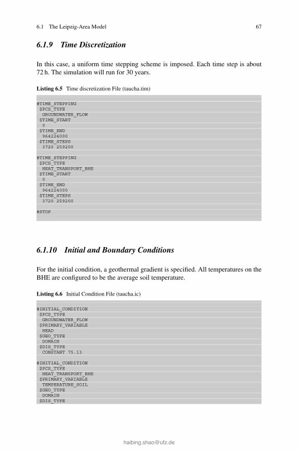
6.1 The Leipzig-Area Model 67
6.1.9 Time Discretization
In this case, a uniform time stepping scheme is imposed. Each time step is about72 h. The simulation will run for 30 years.
Listing 6.5 Time discretization File (taucha.tim)
#TIME_STEPPING$PCS_TYPEGROUNDWATER_FLOW
$TIME_START0
$TIME_END964224000
$TIME_STEPS3720 259200
#TIME_STEPPING$PCS_TYPEHEAT_TRANSPORT_BHE
$TIME_START0
$TIME_END964224000
$TIME_STEPS3720 259200
#STOP
6.1.10 Initial and Boundary Conditions
For the initial condition, a geothermal gradient is specified. All temperatures on theBHE are configured to be the average soil temperature.
Listing 6.6 Initial Condition File (taucha.ic)
#INITIAL_CONDITION$PCS_TYPEGROUNDWATER_FLOW
$PRIMARY_VARIABLEHEAD
$GEO_TYPEDOMAIN
$DIS_TYPECONSTANT 75.13
#INITIAL_CONDITION$PCS_TYPEHEAT_TRANSPORT_BHE
$PRIMARY_VARIABLETEMPERATURE_SOIL
$GEO_TYPEDOMAIN
$DIS_TYPE

68 6 Case Study: A GSHP System in the Leipzig Area
GRADIENT -120 13.32 0.016
#INITIAL_CONDITION$PCS_TYPEHEAT_TRANSPORT_BHE
$PRIMARY_VARIABLETEMPERATURE_IN_1
$GEO_TYPEPOLYLINE ply_BHE0
$DIS_TYPECONSTANT 12.6
#INITIAL_CONDITION$PCS_TYPEHEAT_TRANSPORT_BHE
$PRIMARY_VARIABLETEMPERATURE_OUT_1
$GEO_TYPEPOLYLINE ply_BHE0
$DIS_TYPECONSTANT 12.6
#INITIAL_CONDITION$PCS_TYPEHEAT_TRANSPORT_BHE
$PRIMARY_VARIABLETEMPERATURE_G_1
$GEO_TYPEPOLYLINE ply_BHE0
$DIS_TYPECONSTANT 12.6
#INITIAL_CONDITION$PCS_TYPEHEAT_TRANSPORT_BHE
$PRIMARY_VARIABLETEMPERATURE_G_2
$GEO_TYPEPOLYLINE ply_BHE0
$DIS_TYPECONSTANT 12.6
#STOP
Regarding the boundary condition, a fluctuating surface temperature was spec-ified, which refers to the curve #2 in the RFD file. This curve was generated byconnecting annual temperature curve one after the other.
Listing 6.7 Boundary Condition File (taucha.bc)
#BOUNDARY_CONDITION$PCS_TYPEGROUNDWATER_FLOW
$PRIMARY_VARIABLEHEAD
$GEO_TYPESURFACE inflow
$DIS_TYPECONSTANT 75.4
#BOUNDARY_CONDITION$PCS_TYPEGROUNDWATER_FLOW
$PRIMARY_VARIABLEHEAD

6.1 The Leipzig-Area Model 69
$GEO_TYPESURFACE outflow
$DIS_TYPECONSTANT 74.86
#BOUNDARY_CONDITION$PCS_TYPEHEAT_TRANSPORT_BHE
$PRIMARY_VARIABLETEMPERATURE_IN_1
$GEO_TYPEPOINT BHE0_top
$DIS_TYPECONSTANT 1.0
#BOUNDARY_CONDITION$PCS_TYPEHEAT_TRANSPORT_BHE
$PRIMARY_VARIABLETEMPERATURE_OUT_1
$GEO_TYPEPOINT BHE0_bottom
$DIS_TYPECONSTANT 1.0
#BOUNDARY_CONDITION$PCS_TYPEHEAT_TRANSPORT_BHE
$PRIMARY_VARIABLETEMPERATURE_SOIL
$GEO_TYPESURFACE inflow
$DIS_TYPEGRADIENT -120 13.32 0.016
#BOUNDARY_CONDITION$PCS_TYPEHEAT_TRANSPORT_BHE
$PRIMARY_VARIABLETEMPERATURE_SOIL
$GEO_TYPESURFACE top
$DIS_TYPECONSTANT 1.0
$TIM_TYPECURVE 2
#STOP
Here for the source term, a fixed heat flux term is specified, representing the heatconducted from the deep earth.
Listing 6.8 Source term File (taucha.st)
#SOURCE_TERM$PCS_TYPEHEAT_TRANSPORT_BHE
$PRIMARY_VARIABLETEMPERATURE_SOIL
$GEO_TYPESURFACE bottom
$DIS_TYPECONSTANT_NEUMANN 0.0527
#STOP

70 6 Case Study: A GSHP System in the Leipzig Area
6.1.11 Data RFD File
There are four different curves specified in the RFD file. The first one refers to thebuilding thermal load, which will be applied on the heat pump. The second one isthe surface temperature variation. The third and fourth curve are the COP curves ofthe heat pump. The former one is specified for the heating mode and the latter forthe cooling applications.
Listing 6.9 Data File (taucha.rfd)
; heat pump load#CURVE0 031103999 031104000 -52133695999 -52133696000 -156336287999 -156336288000 -260438879999 -260438880000 -364641471999 -364641472000 -416744063999 -416744064000 -312546655999 -312546656000 -260449247999 -260449248000 -156351839999 -156351840000 054431999 054432000 057023999 057024000 059615999 059616000 062207999 0[...]933120000 -521935711999 -521935712000 -1563938303999 -1563938304000 -2604940895999 -2604940896000 -3646943487999 -3646943488000 -4167946079999 -4167946080000 -3125948671999 -3125948672000 -2604951263999 -2604951264000 -1563953855999 -1563953856000 0956447999 0956448000 0959039999 0959040000 0961631999 0961632000 0964223999 0964224000 -521

6.1 The Leipzig-Area Model 71
; surface temperature#CURVE0 15.512591999 15.512592000 11.745183999 11.745184000 6.507775999 6.507776000 4.6010367999 4.6010368000 2.0412959999 2.0412960000 1.2115551999 1.2115552000 1.0618143999 1.0618144000 10.0720735999 10.0720736000 15.1923327999 15.1923328000 19.3125919999 19.3125920000 22.9628511999 22.9628512000 21.0031103999 21.00[...]933120000 15.51935711999 15.51935712000 11.74938303999 11.74938304000 6.50940895999 6.50940896000 4.60943487999 4.60943488000 2.04946079999 2.04946080000 1.21948671999 1.21948672000 1.06951263999 1.06951264000 10.07953855999 10.07953856000 15.19956447999 15.19956448000 19.31959039999 19.31959040000 22.96961631999 22.96961632000 21.00964223999 21.00964224000 15.51
; Curve for COP 35 deg C floor heating#CURVE-5.0 3.525.0 6.0
; Curve for COP 18 deg C cooling#CURVE5.0 8.030.0 5.0
#STOP

72 6 Case Study: A GSHP System in the Leipzig Area
6.1.12 Fluid Properties
Here two fluid properties are defined. The first one is the groundwater, and thesecond one refers to the refrigerant circulating in the U-tube.
Listing 6.10 Fluid Properties File (taucha.mfp)
; properties of groundwater#FLUID_PROPERTIES$FLUID_TYPELIQUID
$PCS_TYPEGROUNDWATER_FLOW
$DENSITY1 999.25
$VISCOSITY1 1.1929E-03
$SPECIFIC_HEAT_CAPACITY1 4085.9
$HEAT_CONDUCTIVITY1 0.59214
; properties of refrigerant, ethylen glycol 30%#FLUID_PROPERTIES$FLUID_TYPEREFRIGERANT
$PCS_TYPEHEAT_TRANSPORT_BHE
$DENSITY1 1045.4
$VISCOSITY1 3.8315E-03
$SPECIFIC_HEAT_CAPACITY1 3661.7
$HEAT_CONDUCTIVITY1 0.47222
#STOP
6.1.13 Solid Phase Properties
In the MSP file, the thermal conductivity and heat capacity values are defined.Depending on the different type of sediments, these values are also slightly different.
Listing 6.11 Solid Properties File (taucha.msp)
; properties of soil;MG 0 Geschiebemergel#SOLID_PROPERTIES$DENSITY1 1000.0
$THERMALEXPANSION1 0.0

6.1 The Leipzig-Area Model 73
CAPACITY1 2000.0
CONDUCTIVITY1 1.34
;MG 1 Aquifer#SOLID_PROPERTIES$DENSITY1 1000.0
$THERMALEXPANSION1 0.0
CAPACITY1 2500.0
CONDUCTIVITY1 2.40
;MG 2 Stauer#SOLID_PROPERTIES$DENSITY1 1000.0
$THERMALEXPANSION1 0.0
CAPACITY1 2150.0
CONDUCTIVITY1 3.85
; dummy properties for BHE#SOLID_PROPERTIES$DENSITY1 0.0
$THERMALEXPANSION1 0.0
CAPACITY1 0.0
CONDUCTIVITY1 0.0
#STOP
6.1.14 Medium Properties
Here in the medium property file, BHE parameters are defined. Notice that a specialboundary condition is assigned to the BHE, which is the building thermal load.The model will automatically calculate the COP value based the simulated outflowtemperature. Such feature allows a more realistic modelling of the GSHP system.
Listing 6.12 Medium Properties File (taucha.mmp)
;properties of soil;layer 0#MEDIUM_PROPERTIES$GEO_TYPEDOMAIN

74 6 Case Study: A GSHP System in the Leipzig Area
$GEOMETRY_DIMENSION3
$GEOMETRY_AREA1
$POROSITY1 0.0
$PERMEABILITY_TENSORISOTROPIC 5.0E-07
$HEAT_DISPERSION1 0.0 0.0
;layer 1#MEDIUM_PROPERTIES$GEO_TYPEDOMAIN
$GEOMETRY_DIMENSION3
$GEOMETRY_AREA1
$POROSITY1 0.0
$PERMEABILITY_TENSORISOTROPIC 7.2E-04
$HEAT_DISPERSION1 0.0 0.0
;layer 2#MEDIUM_PROPERTIES$GEO_TYPEDOMAIN
$GEOMETRY_DIMENSION3
$GEOMETRY_AREA1
$POROSITY1 0.0
$PERMEABILITY_TENSORISOTROPIC 5.1E-06
$HEAT_DISPERSION1 0.0 0.0
; properties of BHE 0#MEDIUM_PROPERTIES$GEO_TYPE
POLYLINE ply_BHE0$GEOMETRY_DIMENSION
1$GEOMETRY_AREA
1$BOREHOLE_HEAT_EXCHANGERBHE_TYPE
BHE_TYPE_1UBHE_BOUNDARY_TYPE
BHE_BOUND_BUILDING_POWER_IN_WATT_CURVE_FIXED_FLOW_RATEBHE_POWER_IN_WATT_CURVE_IDX
1BHE_HP_HEATING_COP_CURVE_IDX
3BHE_HP_COOLING_COP_CURVE_IDX
4BHE_LENGTH
93BHE_DIAMETER
0.126BHE_REFRIGERANT_FLOW_RATE
2.7E-04BHE_INNER_RADIUS_PIPE

6.2 Simulation Results 75
0.0137BHE_OUTER_RADIUS_PIPE
0.0167BHE_PIPE_IN_WALL_THICKNESS
0.003BHE_PIPE_OUT_WALL_THICKNESS
0.003BHE_FLUID_TYPE
1BHE_FLUID_LONGITUDIAL_DISPERSION_LENGTH
0.0BHE_GROUT_DENSITY
2190.0BHE_GROUT_POROSITY
0.0BHE_GROUT_HEAT_CAPACITY
1735.16BHE_THERMAL_CONDUCTIVITY_PIPE_WALL
0.39BHE_THERMAL_CONDUCTIVITY_GROUT
0.73BHE_PIPE_DISTANCE
0.053
#STOP
6.2 Simulation Results
The evolution of outlet temperatures and COP of both models is shown for thefirst ten years in Fig. 6.3. For the model without heat pump, the COP values arecomputed as a post-processing result based on the BHE outlet temperatures. Thatmeans, the dynamic regulation of the BHE load according to Eqs. (3.1) and (3.2) isnot included in this model. Therefore, we observe much lower outlet temperaturesand COP values, when the heat pump is not considered. This is also reflected in thestatistical distribution of the COP for all heating periods, which is shown in Fig. 6.4.
The consumption of electrical energy by the heat pump can be computed by
Eel DZ PQBHE.t/
COP.t/dt: (6.4)
With an assumed electricity price of 0.28 Euro kWh�1, the operational costs for theGSHP system evaluate to 29,994 Euro. For the model without heat pump integration,the operational costs evaluate to 43,067 Euro. Please note, that the computation ofCOP evolution and operational costs for the model without heat pump are carriedout here only for demonstration purposes. As can be clearly seen, evaluation ofthese values leads to completely wrong results, as the COP-corrected dynamic loadboundary condition is missing.
As an exemplary results, the soil temperature distribution on a cross-section atthe BHE location after 30 years of operation is shown in Fig. 6.5.

76 6 Case Study: A GSHP System in the Leipzig Area
t/[years]
0 2 4 6 8 10
T/[°
C]
-5
0
5
10
15
20
CO
P/[-]
1
2
3
4
5
6Tout w/ HPTout w/o HPCOP w/ HPCOP w/o HP
Fig. 6.3 Evolution of BHE outlet temperatures and COP
w/ HP w/o HP
CO
P/[-]
3.4
3.6
3.8
4.0
4.2
4.4
4.6
4.8
5.0
Fig. 6.4 Statistical distribution of COP

6.3 Implifications of the Model 77
Fig. 6.5 Soil temperature distribution after 30 years of operation
6.3 Implifications of the Model
6.3.1 Overall Dynamics of the BHE Coupled GSHP System
Figure 6.3 shows the dynamics of BHE outflow temperature over a 10 years of time.Within a heating period, the soil surrounding the BHE will first be cooled, this alsoleads to a cold plume around the BHE (cf. Fig. 6.5). Along with the temperaturedrop, a steep gradient will form between the BHE and the soil in the vicinity ofit. This means, the heat transfer process will be enhanced, and sensible heat in thesubsurface will be driven by such gradient and eventually be collected by the BHE.If the BHE keeps extracting heat, the size of the plume will increase, until a quasisteady-state is reached, i.e. the soil temperature distribution only changes very littleover time. As illustrated in Fig. 6.3, once the heating period is over, the heat willstill be driven by the gradient, to make the soil temperature to recover.
6.3.2 The Role of the Heat Pump
It should be noticed that, for a realistic simulation of the GSHP system, the heatpump dynamics is also an essential part and cannot be ignored. As shown inFig. 6.3, when the heat pump is involved, the modelled outflow temperature will beconsistently higher than the profile without it. This is because, the heat pump acts asa buffer between the building thermal load and the BHE. When a strong thermal load

78 6 Case Study: A GSHP System in the Leipzig Area
is imposed on the BHE, the outflow temperature will drop in response. Meanwhile,the heat pump efficiency, in terms of COP value, will also drop correspondingly.This means, more heat will be supplied by the electricity consumption, rather anheat extracted from the subsurface. As a result, the outflow temperature in the reality,where a heat pump is always coupled, will be higher than the simulated scenario, inwhich the building thermal load is directly imposed on the BHE.
6.3.3 The Price of Under-Design
With the above heat pump featured in mind, one may argue that under-designof the BHE system might be beneficial. Since electricity price in many countiesis relatively low, and drilling cost is very high. It could be an overall beneficialchoice, to save on the initial investment by drilling a shorter BHE, and pay moreon the electricity bill over years. By using the Leipzig-area model presentedabove, a numerical experiment has been conducted. Here, the engineers wereassumed to have designed the BHE system based on a soil thermal conductivityvalue of 2.4 W m�1 K�1, while the actual lambda values is only 2.1, 1.8, 1.5 and1.2 W m�1 K�1. The corresponding minimum outflow and soil temperature profileswere depicted in Fig. 6.6. It can be observed that, with a lower real lambda value, theoutflow temperature every year will be considerably lower. One could imagine, that
t/[years]2 4 6 8 10 12 14 16 18 20 22 24 26 28 30
T out,m
in/[°
C]
-5
0
5
10
T soil,
min/[°
C]
0
5
10
15λeff = 1.2 Wm-1K-1
λeff = 1.5 Wm-1K-1
λeff = 1.8 Wm-1K-1
λeff = 2.1 Wm-1K-1
λeff = 2.4 Wm-1K-1
Fig. 6.6 Evolution of minimum soil and outflow temperature, by incorrectly assumed thermalconductivity values of the subsurface (under-design scenarios after Hein et al. 2016)

6.3 Implifications of the Model 79
the heat pump will be running under an unfavourable condition. More importantly,with a severe under-design, the outflow temperature can drop down to as low as�5 ıC. For most heat pump systems, such a sharp drop in the outflow temperaturewill cause a sudden system shut-down during the cold winter. Therefore, a site-specific subsurface investigation will be essential to the long-term success of BHEcoupled GSHP system.

Chapter 7Summary and Outlook
After talking a lot about how to numerically model the heat transport processinduced by a GSHP system, a few advices can be given to the end users, whichwere obtained by the authors through various modelling studies.
• Before designing a GSHP system, it is recommended to obtain the subsurfacecharacteristics as accurately as possible. For example, the identification ofaquifer and groundwater can greatly enhance the efficiency of the borehole heatexchangers, leading to a much shorter BHE and lower drilling cost. On the otherside, if the thermal conductivity of the soil is over-estimated, a under-designedsystem can quickly run into trouble after a few years of operation.
• Make sure to conduct proper grouting inside the BHE. This is not only requiredby the regulation to prevent groundwater contamination. Actually, a poorlygrouted BHE with air pocket in it is eventually a BHE with smaller surface areafor heat exchange. When possible, a thermally enhanced grout should be applied,as simulation based result suggests that the additional investment will quickly bepaid off after couple of years’ operation (cf. Hein et al. 2016).
• Try to avoid multiple BHEs located in a close vicinity. The distance betweenBHEs is recommended to be larger than 10 m. Simulation results has suggestedthat the thermal plume from adjacent BHEs is very likely to interfere with eachother. There are cases where the BHEs are drilled very close to each other andthe system performance starts to drop after a few years of operation.
As mentioned above, more and more commercial buildings are now equipped withBHE coupled GSHP systems. In such cases, often dozens or even hundreds of BHEsare connected to each other and drilled in a small piece of land. These big systemscan not be simulated yet by the OpenGeoSys software in its current stage. Currently,research has already been started on this front, and readers could expect an updatedtutorial focusing on this topic in the near future.
© The Author(s) 2016H. Shao et al., Geoenergy Modeling II, SpringerBriefs in Energy,DOI 10.1007/978-3-319-45057-5_7
81

Appendix ASymbols
The symbols used in the tutorial is summarized in Table A.1.
Table A.1 Table of Symbols Symbol Parameter Unit
Latin symbols
A Global system matrix
a Heat transfer coefficient W � K�1 � m�2
b Right-hand-side vector
c Specific heat capacity J � kg�1 � K�1
Cr Courant number, criteria
D Diagonal matrix
e Specific energy J � kg�1
ek Iteration error
g Gravity acceleration vector m � s�1
h Specific enthalpy J � kg�1
jadv Advective heat flux W � m�2
jdiff Diffusive heat flux W � m�2
jdisp Dispersive heat flux W � m�2
J Jacobian
k Permeability tensor m2
krel Relative permeability �K.e/ Element conductivity matrix
L Differential operatorOL Approximation operator
L Lower matrix
L.e/ Element length
m Mass kg
n Porosity m3 � m�3
N.e/ Element shape function
Ne Neumann number, criteria
© The Author(s) 2016H. Shao et al., Geoenergy Modeling II, SpringerBriefs in Energy,DOI 10.1007/978-3-319-45057-5
83

84 A Symbols
Symbol Parameter Unit
qi Internal heat source J kg�1 s�1
q Darcy flux, velocity m s�1
Q Amount of heat J
QT Heat production term (volumetric) J m�3 s�1
qT Heat production term (specific) kg�1 s�1
R Residuum vector
S Saturation �t Time s
T Temperature K
u Internal energy J kg�1
u.t; x/ Unknown field function of time and space
unj Unknown field function approximation at time level n in node j
U Upper matrix
v Velocity vector m s�1
V Volume m3
x Solution vector
Greek symbols
˛ Diffusivity m2 s�1
� Thermal conductivity W K�1 m�1
� Density kg m�3
Difference �� Volume fraction ��n
j Approximation error at time level n in node j � Conservation quantity �� Stress tensor Pa
� Viscosity Pa s
Exponents, indices
i; j Node numbers
k Non-linear iteration number
n Time level
s Solid
l Liquid
w Water
f Fluid
˛ All phases
� Fluid phases

Appendix BKeywords
This section provides a wrap-up compendium of the OGS keywords used in thistutorial. A more comprehensive compilation of OGS keywords you can find at www.opengeosys.org/help/documentation/.
B.1 GLI: Geometry
Listing B.1 GLI keyword
#POINTS // points keyword0 0 0 0 $NAME POINT0 // point number | x | y | z | point name1 1 0 0 $NAME POINT1 // point number | x | y | z | point name#POLYLINE // polyline keyword$NAME // polyline name subkeywordLINE // polyline name
$POINTS // polyline points subkeyword0 // point of polyline1 // dito
#STOP // end of input data
OGS Weblink:http://www.opengeosys.org/help/documentation/geometry-file
B.2 MSH: Finite Element Mesh
Listing B.2 MSH keyword
#FEM_MSH // file/object keyword$NODES // node subkeyword61 // number of grid nodes0 0 0 0 // node number x y z
© The Author(s) 2016H. Shao et al., Geoenergy Modeling II, SpringerBriefs in Energy,DOI 10.1007/978-3-319-45057-5
85

86 B Keywords
1 0 0 1 // dito...59 0 0 5960 0 0 60$ELEMENTS // element subkeyword60 // number of elements0 0 line 0 1 // element number | material group number |
element type | element node numbers1 0 line 1 2 // dito...58 0 line 58 59 // dito59 0 line 59 60 // dito#STOP // end of input data
OGS Weblink:http://www.opengeosys.org/help/documentation/mesh-file
B.3 PCS: Process Definition
Listing B.3 PCS keyword
#PROCESS // process keyword$PCS_TYPE // process type subkeyword
HEAT_TRANSPORT // specified process(es)GROUNDWATER_FLOW // ditoLIQUID_FLOW // dito
...#STOP // end of input data
OGS Weblink:www.opengeosys.org/help/documentation/process-file
B.4 NUM: Numerical Properties
Listing B.4 NUM keyword
#NUMERICS // process keyword$PCS_TYPE // process type subkeyword, see PCS above$LINEAR_SOLVER // linear solver type subkeyword, see table below
Parameters // 7 parameters, see table below#STOP // end of input data
Numerical properties
• Linear solver type (its C++ ;-) numbering �1)
1. SpGAUSS, direct solver2. SpBICGSTAB

B.5 TIM: Time Discretization 87
3. SpBICG4. SpQMRCGSTAB5. SpCG6. SpCGNR7. CGS8. SpRichard9. SpJOR
10. SpSOR
• Convergence criterion (its C++ ;-) numbering �1)
1. Absolutely error jjrjj < �2. jjrjj < �jjbjj3. jjrnjj < �jjrn � 1jj4. if jjrnjj < 1 then jjrnjj < �jjrn � 1jj else jjrjj < �5. jjrnjj < �jjxjj6. jjrnjj < �max jjrn � 1jj; jjxjj; jjbjj
• Error tolerance �, according to the convergence criterion model above• Maximal number of linear solver iterations• Relaxation parameter 2 Œ0; 1�• Preconditioner
0 No preconditioner,1 Jacobi preconditioner,100 ILU preconditioner.
• Storage model
2 unsymmetrical matrix,4 symmetrical matrix.
OGS Weblink:http://www.opengeosys.org/help/documentation/numeric-file
B.5 TIM: Time Discretization
Listing B.5 TIM keyword
#TIME_STEPPING // time stepping keyword$PCS_TYPE // process subkeyword
HEAT_TRANSPORT // specified process$TIME_STEPS // time steps subkeyword1000 390625e+0 // number of times steps | times step length
$TIME_END // end time subkeyword1E99 // end time value
$TIME_START // starting time subkeyword

88 B Keywords
0.0 // starting time value$TIME_UNIT // specified time unit
DAY // SECOND, DAY, YEAR#STOP // end of input data
OGS Weblink:http://www.opengeosys.org/help/documentation/time-step-control-file
B.6 IC: Initial Conditions
Listing B.6 IC keyword
#INITIAL_CONDITION // initial conditions keyword$PCS_TYPE // process subkeywordHEAT_TRANSPORT // specified process
$PRIMARY_VARIABLE // primary variable subkeywordTEMPERATURE1 // specified primary variable
$GEO_TYPE // geometry subkeywordDOMAIN // specified geometry: entire domain (all nodes)
$DIS_TYPE // distribution subkeywordCONSTANT 0 // specified distribution: constant value 0 at DOMAIN
geometry#STOP // end of input data
OGS Weblink:http://www.opengeosys.org/help/documentation/initial-condition-file
B.7 BC: Boundary Conditions
Listing B.7 BC keyword
#BOUNDARY_CONDITION // boundary condition keyword$PCS_TYPE // process type subkeywordHEAT_TRANSPORT // specified process
$PRIMARY_VARIABLE // primary variable subkeywordTEMPERATURE1 // specified primary variable
$GEO_TYPE // geometry type subkeywordPOINT POINT0 // specified geometry type | geometry name
$DIS_TYPE // boundary condition type subkeywordCONSTANT 1 // boundary condition type | value
#STOP // end of input data
OGS Weblink:http://www.opengeosys.org/help/documentation/boundary-condition-file

B.9 MFP: Fluid Properties 89
B.8 ST: Source/Sink Terms
Listing B.8 ST keyword
#SOURCE_TERM // source term keyword$PCS_TYPE // process type subkeywordLIQUID_FLOW // specified process
$PRIMARY_VARIABLE // primary variable subkeywordPRESSURE1 // specified primary variable
$GEO_TYPE // geometry type subkeywordPOINT POINT0 // specified geometry type | geometry name
$DIS_TYPE // boundary condition type subkeywordCONSTANT_NEUMANN 1E-6 // source term type | value
#STOP // end of input data
OGS Weblink:http://www.opengeosys.org/help/documentation/source-term-file
B.9 MFP: Fluid Properties
Listing B.9 MFP keyword
#FLUID_PROPERTIES // fluid properties keyword$DENSITY // fluid density subkeyword4 1000 0 -0.2 // type (4: temperature dependent) | 2 values
$VISCOSITY // fluid viscosity subkeyword1 0.001 // type (1: constant value) | value
$SPECIFIC_HEAT_CAPACITY // specific heat capacity subkeyword1 4200.0 // type (1: constant value) | value
$HEAT_CONDUCTIVITY // thermal heat conductivity subkeyword1 0.65 // type (1: constant value) | value
#STOP // end of input data
OGS Weblink:http://www.opengeosys.org/help/documentation/fluid-properties-fileSee Table B.1.
Table B.1 Density models
Model Meaning Formula Parameters
0 Curve RFD file
1 Constant value �0 Value of �02 Pressure dependent �.p/ D �0.1C ˇp.p � p0// �0; ˇp; p03 Salinity dependent �.C/ D �0.1C ˇC.C � C0// �0; ˇp;C04 Temperature dependent �.p/ D �0.1C ˇT .T � T0// �0; ˇT ;T0: : : : : : : : : : : :

90 B Keywords
B.10 MSP: Solid Properties
Listing B.10 MSP keyword
#SOLID_PROPERTIES // solid properties keyword$DENSITY // solid density subkeyword
1 2500 // type (1: constant value) | value$THERMAL // thermal properties subkeyword
EXPANSION: // thermal expansion1.0e-5 // values
CAPACITY: // heat capacity1 1000 // type (1: constant value) | value
CONDUCTIVITY: // thermal conductivity1 3.2 // type (1: constant value) | value
#STOP // end of input data
OGS Weblink:TBD
B.11 MMP: Porous Medium Properties
Listing B.11 MMP keyword
#MEDIUM_PROPERTIES // solid properties keyword$GEOMETRY_DIMENSION // dimension subkeyword1 // 1: one-dimensional problem
$GEOMETRY_AREA // geometry area subkeyword1.0 // value in square meter if 1D
$POROSITY // porosity subkeyword1 0.10 // type (1: constant value) | value
$STORAGE // storativity subkeyword1 0.0 // type (1: constant value) | value
$TORTUOSITY // tortuosity subkeyword1 1.000000e+000 // type (1: constant value) | value
$PERMEABILITY_TENSOR // permeability subkeywordISOTROPIC 1.0e-15 // tensor type (ISOTROPIC) | value(s)
$HEAT_DISPERSION // porosity subkeyword1 0.0e+00 0.0e+00 // type (1: constant values) | longitudinal |
transverse// thermal dispersion length
#STOP // end of input data
OGS Weblink:http://www.opengeosys.org/help/documentation/material-properties-file

B.12 OUT: Output Parameters 91
B.12 OUT: Output Parameters
Listing B.12 OUT keyword
#OUTPUT // output keyword$PCS_TYPE // process subkeywordHEAT_TRANSPORT // specified process
$NOD_VALUES // nodal values subkeywordTEMPERATURE1 // specified nodal values
$GEO_TYPE // geometry type subkeywordPOLYLINE ROCK // geometry type and name
$TIM_TYPE // output times subkeywordSTEPS 1 // output methods and parameter
#STOP // end of input data
OGS Weblink:http://www.opengeosys.org/help/documentation/output-control-file

References
Al-Khoury, R., Kölbel, T., Schramedei, R.: Efficient numerical modeling of borehole heatexchangers. Comput. Geosci. 36(10), 1301–1315 (2010). ISSN 0098-3004. doi:http://dx.doi.org/10.1016/j.cageo.2009.12.010
Arola, T., Korkka-Niemi, K.: The effect of urban heat islands on geothermal potential: examplesfrom quaternary aquifers in finland. Hydrogeol. J. 22(8), 1953–1967 (2014). ISSN 1435-0157.doi:10.1007/s10040-014-1174-5
Bauer, S., Beyer, C., Dethlefsen, F., Dietrich, P., Duttmann, R., Ebert, M., Feeser, V., Görke, U.,Köber, R., Kolditz, O., Rabbel, W., Schanz, T., Schäfer, D., Würdemann, H., Dahmke, A.:Impacts of the use of the geological subsurface for energy storage: an investigation concept.Environ. Earth Sci. 70(8), 3935–3943 (2013)
Beier, R.A., Smith, M.D., Spitler, J.D.: Reference data sets for vertical borehole ground heatexchanger models and thermal response test analysis. Geothermics 40(1), 79–85 (2011).doi:10.1016/j.geothermics.2010.12.007
Cacace, M., Blöcher, G., Watanabe, N., Moeck, I., Börsing, N., Scheck-Wenderoth, M., Kolditz,O., Huenges, E.: Modelling of fractured carbonate reservoirs: outline of a novel technique viaa case study from the molasse basin, southern bavaria, germany. Environ. Earth Sci. 70(8),3585–3602 (2013)
Casasso, A., Sethi, R.: Efficiency of closed loop geothermal heat pumps: a sensitivity analysis.Renew. Energy 62, 737–746 (2014)
Clauser, C.: Thermal Signatures of Heat Transfer Processes in the Earth’s Crust. Springer,Heidelberg (1999). ISBN 3-540-65604-9
Diersch, H.-J.G., Bauer, D., Heidemann, W., Rühaak, W., Schätzl, P.: Finite element modeling ofborehole heat exchanger systems: part 1. Fundamentals. Comput. Geosci. 37(8), 1122–1135(2011a). ISSN 0098-3004. doi:http://dx.doi.org/10.1016/j.cageo.2010.08.003
Diersch, H.-J.G., Bauer, D., Heidemann, W., Rühaak, W., Schätzl, P.: Finite element modelingof borehole heat exchanger systems: part 2. Numerical simulation. Comput. Geosci. 37(8),1136–1147 (2011b). ISSN 0098-3004. doi:http://dx.doi.org/10.1016/j.cageo.2010.08.003
Diersch, H.-J.: FEFLOW Finite Element Modeling of Flow, Mass and Heat Transport in Porousand Fractured Media. Springer, Heidelberg (2014)
Eicker, U., Vorschulze, C.: Potential of geothermal heat exchangers for office building climatisa-tion. Renew. Energy 34(4), 1126–1133 (2009).
Glen Dimplex Deutschland GmbH: Heat pump SI30TER+, equipment data (2016). http://www.dimplex.de/pdf/de/produktattribute/produkt_1722822_extern_egd.pdf
© The Author(s) 2016H. Shao et al., Geoenergy Modeling II, SpringerBriefs in Energy,DOI 10.1007/978-3-319-45057-5
93

94 References
Hein, P., Kolditz, O., Görke, U.-J., Bucher, A., Shao, H.: A numerical study on the sustainabilityand efficiency of borehole heat exchanger coupled ground source heat pump systems. Appl.Therm. Eng. 100, 421–433 (2016). ISSN 1359–4311. doi:http://dx.doi.org/10.1016/j.applthermaleng.2016.02.039
Huenges, E., Kohl, T., Kolditz, O., Bremer, J., Scheck-Wenderoth, M., Vienken, T.: Geothermalenergy systems: research perspective for domestic energy provision. Environ. Earth Sci. 70(8),3927–3933 (2013)
Jaszczur, M., Sliwa, T.: The analysis of long-term borehole heat exchanger system exploitation.Comput. Assist. Methods Eng. Sci. 20(3), 227–235 (2013)
Kahraman, A., Çelebi, A.: Investigation of the performance of a heat pump using waste water as aheat source. Energies 2(3), 697–713 (2009)
Kolditz, O., Jakobs, L.A., Huenges, E., Kohl, T.: Geothermal energy: a glimpse at the state of thefield and an introduction to the journal. Geotherm. Energy 1 (2013). doi:10.1186/2195-9706-1-1
Leipzig Institute for Meteorology - LIM, Faculty of Physics and Earth Sciences, UniversityLeipzig: Weather and climate archive data (Wetter & Klima, Archivdaten) (2016). http://www.uni-leipzig.de/~meteo/en/wetterdaten/archiv.php
Panteleit, B., Reichling, J.: Automatical assignement of petrographic parameters for optimizedground-source heat pumps (Automatisierte Attribuierung von Bohrungsdaten mit Parame-tern zur Optimierung von Erdwärmesondenanlagen). Grundwasser 11(1), 19–26 (2006).doi:10.1007/s00767-006-0115-1
Richter, M., Huber, C., Reinhardt, K., Wachmann, H., Gerschel, A.: Potential of heat sup-ply for Saxon gardening companies utilizing geothermal energy as subject to site-specificgeological conditions and different business organisations/utilisation concepts (Möglichkeitender Wärmeversorgung von sächsischen Gartenbaubetrieben mit Geothermie in Abhängigkeitvon geologischen Standortfaktoren und verschiedenen Betriebsstrukturen/Nutzungskonzepten)(2015)
Sanner, B., Karytsas, C., Mendrinos, D., Rybach, L.: Current status of ground source heat pumpsand underground thermal energy storage in europe. Geothermics 32(4), 579–588 (2003)
Scheck-Wenderoth, M., Schmeisser, D., Mutti, M., Kolditz, O., Huenges, E., Schultz, H.-M.,Liebscher, A., Bock, M.: Geoenergy: new concepts for utilization of geo-reservoirs as potentialenergy sources. Environ. Earth Sci. 70(8), 3427–3431 (2013)
Speer, S.: Design calculations for optimising of a deep borehole heat-exchanger. Master’s thesis,RWTH Aachen University, Aachen (2005)
Stauffer, F., Bayer, P., Blum, P., Molina-Giraldo, N., Kinzelbach, W.: Thermal Use of ShallowGroundwater. Taylor & Francis Group, Boca Raton (2014)
The Association of German Engineers (Verein Deutscher Ingenieure): VDI guideline 4640: ther-mal use of the underground – part 2: ground source heat pump systems, draft (VDI Richtlinie4640: Thermische Nutzung des Untergrunds - Blatt 2: Erdgekoppelte Wärmepumpenanlagen,Entwurf) (2015)
Zheng, T., Shao, H., Schelenz, S., Hein, P., Vienken, T., Pang, Z., Kolditz, O., Nagel, T.: Efficiencyand economic analysis of utilizing latent heat from groundwater freezing in the context ofborehole heat exchanger coupled ground source heat pump systems. Appl. Therm. Eng. 105,314–326 (2016). ISSN 1359–4311. doi:http://dx.doi.org/10.1016/j.applthermaleng.2016.05.158
Zhu, K., Blum, P., Ferguson, G., Balke, K.-D., Bayer, P.: The geothermal potential of urban heatislands. Environ. Res. Lett. 5(4), 044002 (2010)