H. Pang / NUS

Principles of Query Processing

Pang Hwee Hwa

School of Computing, NUS

CS5226 Week 5

H. Pang / NUS

ApplicationProgrammer

(e.g., business analyst,Data architect)

SophisticatedApplicationProgrammer

(e.g., SAP admin)

DBA,Tuner

Hardware[Processor(s), Disk(s), Memory]

Operating System

Concurrency Control Recovery

Storage SubsystemIndexes

Query Processor

Application

H. Pang / NUS

Overview of Query Processing

Parser QueryOptimizer

Statistics Cost Model

QEPParsed Query

Database

High Level Query Query Result

QueryEvaluator

H. Pang / NUS

Outline

• Processing relational operators

• Query optimization

• Performance tuning

H. Pang / NUS

Projection Operator

R.attrib, .. (R)

• Implementation is straightforward

SELECT bidFROM Reserves RWHERE R.rname < ‘C%’

H. Pang / NUS

Selection Operator

R.attr op value (R)

• Size of result = R * selectivity • Scan• Clustered index: Good• Non-clustered index:

– Good for low selectivity– Worse than scan for high selectivity

SELECT *FROM Reserves RWHERE R.rname < ‘C%’

H. Pang / NUS

Example of Join

sid sname rating age22 dustin 7 45.028 yuppy 9 35.031 lubber 8 55.544 guppy 5 35.058 rusty 10 35.0

sid bid day rname

31 101 10/11/96 lubber58 103 11/12/96 dustin

sid sname rating age bid day rname

31 lubber 8 55.5 101 10/11/96 lubber58 rusty 10 35.0 103 11/12/96 dustin

SELECT *FROM Sailors R, Reserve SWHERE R.sid=S.sid

H. Pang / NUS

Notations

• |R| = number of pages in outer table R• ||R|| = number of tuples in outer table R• |S| = number of pages in inner table S• ||S|| = number of tuples in inner table S• M = number of main memory pages allocated

H. Pang / NUS

Simple Nested Loop Join

R S

Tuple

1 scan per R tuple

|S| pages per scan||R|| tuples

H. Pang / NUS

Simple Nested Loop Join

• Scan inner table S per R tuple: ||R|| * |S|– Each scan costs |S| pages– For ||R|| tuples

• |R| pages for outer table R• Total cost = |R| + ||R|| * |S| pages• Not optimal!

H. Pang / NUS

Block Nested Loop Join

R S

M – 2 pages

1 scan per R block

|S| pages per scan|R| / (M – 2) blocks

H. Pang / NUS

Block Nested Loop Join

• Scan inner table S per block of (M – 2) pages of R tuples– Each scan costs |S| pages– |R| / (M – 2) blocks of R tuples

• |R| pages for outer table R

• Total cost = |R| + |R| / (M – 2) * |S| pages

• R should be the smaller table

H. Pang / NUS

Index Nested Loop Join

R S

Tuple

Index

||R|| tuples

1 probe per R tuple

H. Pang / NUS

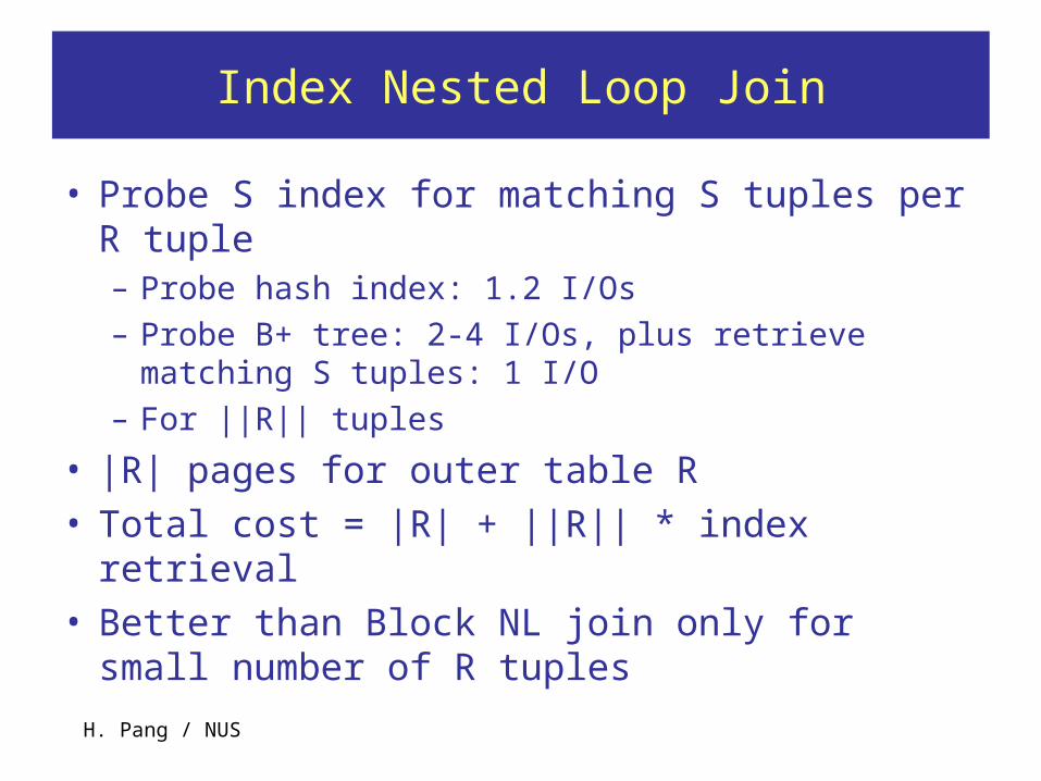
Index Nested Loop Join

• Probe S index for matching S tuples per R tuple– Probe hash index: 1.2 I/Os– Probe B+ tree: 2-4 I/Os, plus retrieve matching S

tuples: 1 I/O– For ||R|| tuples

• |R| pages for outer table R• Total cost = |R| + ||R|| * index retrieval• Better than Block NL join only for small number

of R tuples

H. Pang / NUS

Sort Merge Join

• External sort R• External sort S• Merge sorted R and sorted S

H. Pang / NUS

External Sort R

R0,M-1 R0,M… …

R1,2 R1,M-1…Merge pass 1 R1,1

Merge pass 2 R2,1

Split pass R R0,1

# merge passes = logM-1 |R|/M

Cost per pass = |R| input + |R| output = 2 |R|

Total cost = 2 |R| (logM-1 |R|/M + 1) including split pass

Size of R0,i = M, # R0,i’s = |R|/M

(m-1)-waymerge

H. Pang / NUS

Sort Merge Join

• External-sort R: 2 |R| * (logM-1 |R|/M + 1)– Split R into |R|/M sorted runs each of size M: 2 |R|– Merge up to (M – 1) runs repeatedly logM-1 |R|/M passes, each costing 2 |R|

• External-sort S: 2 |S| * (logM-1 |S|/M + 1)• Merge matching tuples from sorted R and S: |R|

+ |S|• Total cost = 2 |R| * (logM-1 |R|/M + 1) + 2 |S| *

(logM-1 |S|/M + 1) + |R| + |S|– If |R| < M*(M-1), cost = 5 * (|R| + |S|)

H. Pang / NUS

GRACE Hash Join

X X XX X X X X X X X X X X X X X X X X X X X X X X X X X X X X X X X X

R

S

0

1

2

3

0 1 2 3

bucketID = X mod 4Join on R.X = S.X

R S = R0 S0 + R1 S1 + R2 S2 + R3 S3

H. Pang / NUS

GRACE Hash Join – Partition Phase

M main memory buffers DiskDisk

Original Relation OUTPUT

2INPUT

1

hashfunction

h1M-1

Partitions

1

2

M-1

. . .

R (M – 1) partitions, each of size |R| / (M – 1)

H. Pang / NUS

GRACE Hash Join – Join Phase

Partitionsof R & S

Input bufferfor Si

Hash table for partitionRi (< M-1 pages)

B main memory buffersDisk

Output buffer

Disk

Join Result

hashfnh2

h2

Partition must fit in memory: |R| / (M – 1) < M -1

H. Pang / NUS

GRACE Hash Join Algorithm

• Partition phase: 2 (|R| + |S|)– Partition table R using hash function h1: 2 |R|– Partition table S using hash function h1: 2 |S|– R tuples in partition i will match only S tuples in partition I– R (M – 1) partitions, each of size |R| / (M – 1)

• Join phase: |R| + |S|– Read in a partition of R (|R| / (M – 1) < M -1)– Hash it using function h2 (<> h1!)– Scan corresponding S partition, search for matches

• Total cost = 3 (|R| + |S|) pages

• Condition: M > √f|R|, f ≈ 1.2 to account for hash table

H. Pang / NUS

Summary of Join Operator

• Simple nested loop: |R| + ||R|| * |S|

• Block nested loop: |R| + |R| / (M – 2) * |S|

• Index nested loop: |R| + ||R|| * index retrieval

• Sort-merge: 2 |R| * (logM-1 |R|/M + 1) + 2 |S| *

(logM-1 |S|/M + 1) + |R| + |S|

• GRACE hash: 3 * (|R| + |S|)– Condition: M > √f|R|

H. Pang / NUS

Overview of Query Processing

Parser QueryOptimizer

Statistics Cost Model

QEPParsed Query

Database

High Level Query Query Result

QueryEvaluator

H. Pang / NUS

Query Optimization

• Given: An SQL query joining n tables• Dream: Map to most efficient plan• Reality: Avoid rotten plans• State of the art:

– Most optimizers follow System R’s technique– Works fine up to about 10 joins

SELECT S.snameFROM Reserves R, Sailors SWHERE R.sid=S.sid AND R.bid=100 AND S.rating>5

Reserves Sailors

sid=sid

bid=100 rating > 5

sname

H. Pang / NUS

Complexity of Query Optimization

• Many degrees of freedom– Selection: scan versus

(clustered, non-clustered) index

– Join: block nested loop, sort-merge, hash

– Relative order of the operators

– Exponential search space!

• Heuristics– Push the selections down– Push the projections down– Delay Cartesian products– System R: Only left-deep

trees

BA

C

D

H. Pang / NUS

• Selection: - cascade

- commutative

• Projection: - cascade

• Join: - associative

- commutative

Equivalences in Relational Algebra

c cn c cnR R1 1 ... . . .

c c c cR R1 2 2 1

a a anR R1 1 . . .

R (S T) (R S) T

(R S) (S R)

H. Pang / NUS

Equivalences in Relational Algebra

• A projection commutes with a selection that only uses attributes retained by the projection

• Selection between attributes of the two arguments of a cross-product converts cross-product to a join

• A selection on just attributes of R commutes with join R S (i.e., (R S) (R) S )

• Similarly, if a projection follows a join R S, we can `push’ it by retaining only attributes of R (and S) that are needed for the join or are kept by the projection

H. Pang / NUS

System R Optimizer

1. Find all plans for accessing each base table2. For each table

• Save cheapest unordered plan• Save cheapest plan for each interesting order• Discard all others

3. Try all ways of joining pairs of 1-table plans; save cheapest unordered + interesting ordered plans

4. Try all ways of joining 2-table with 1-table5. Combine k-table with 1-table till you have full plan tree6. At the top, to satisfy GROUP BY and ORDER BY

• Use interesting ordered plan• Add a sort node to unordered plan

H. Pang / NUS Source: Selinger et al, “Access Path Selection in a Relational Database Management System”

H. Pang / NUS

Note: Only branches for NL join are shown here. Additional branches for other join methods (e.g. sort-merge) are not shown.

Source: Selinger et al, “Access Path Selection in a Relational Database Management System”

H. Pang / NUS

What is “Cheapest”?

• Need information about the relations and indexes involved

• Catalogs typically contain at least:– # tuples (NTuples) and # pages (NPages) for each relation.– # distinct key values (NKeys) and NPages for each index.– Index height, low/high key values (Low/High) for each tree index.

• Catalogs updated periodically.– Updating whenever data changes is too expensive; lots of

approximation anyway, so slight inconsistency ok.

• More detailed information (e.g., histograms of the values in some field) are sometimes stored.

H. Pang / NUS

Estimating Result Size

• Consider a query block:

• Maximum # tuples in result is the product of the cardinalities of relations in the FROM clause.

• Reduction factor (RF) associated with each termi reflects the impact of the term in reducing result size– Term col=value has RF 1/NKeys(I)– Term col1=col2 has RF 1/MAX(NKeys(I1), NKeys(I2))– Term col>value has RF (High(I)-value)/(High(I)-Low(I))

• Result cardinality = Max # tuples * product of all RF’s.– Implicit assumption that terms are independent!

SELECT attribute listFROM relation listWHERE term1 AND ... AND termk

H. Pang / NUS

Cost Estimates for Single-Table Plans

• Index I on primary key matches selection:– Cost is Height(I)+1 for a B+ tree, about 1.2 for hash index.

• Clustered index I matching one or more selects:– (NPages(I)+NPages(R)) * product of RF’s of matching selects.

• Non-clustered index I matching one or more selects:– (NPages(I)+NTuples(R)) * product of RF’s of matching selects.

• Sequential scan of file:– NPages(R).

Note: Typically, no duplicate elimination on projections! (Exception: Done on answers if user says DISTINCT.)

H. Pang / NUS

Counting the Costs

• With 5 buffers, cost of plan:– Scan Reserves (1000) + write temp

T1 (10 pages, if we have 100 boats, uniform distribution)

– Scan Sailors (500) + write temp T2 (250 pages, if we have 10 ratings).

– Sort T1 (2*10*2), sort T2 (2*250*4), merge (10+250), total=2300

– Total: 4060 page I/Os

• If we used BNL join, join cost = 10+4*250, total cost = 2770

• If we ‘push’ projections, T1 has only sid, T2 only sid and sname:– T1 fits in 3 pages, cost of BNL

drops to under 250 pages, total < 2000

Reserves Sailors

sid=sid

bid=100

sname(On-the-fly)

rating > 5(Scan;write to temp T1)

(Scan;write totemp T2)

(Sort-Merge Join)

SELECT S.snameFROM Reserves R, Sailors SWHERE R.sid=S.sid AND R.bid=100 AND S.rating>5

H. Pang / NUS

Exercise

• Reserves: 100,000 tuples, 100 tuples per page

• With clustered index on bid of Reserves, we get 100,000/100 = 1000 tuples on 1000/100 = 10 pages

• Join column sid is a key for Sailors - at most one matching tuple

• Decision not to push rating>5 before the join is based on availability of sid index on Sailors

• Cost: Selection of Reserves tuples (10 I/Os); for each tuple, must get matching Sailors tuple (1000*1.2); total 1210 I/Os

Reserves

Sailors

sid=sid

bid=100

sname(On-the-fly)

rating > 5

(Use clustered index on sid)

(Index Nested Loops,with pipelining )

(On-the-fly)

(Use hashIndex on sid)

H. Pang / NUS

Query Tuning

H. Pang / NUS

Avoid Redundant DISTINCT

• DISTINCT usually entails a sort operation• Slow down query optimization because one

more “interesting” order to consider• Remove if you know the result has no duplicates

SELECT DISTINCT ssnumFROM EmployeeWHERE dept = ‘information systems’

H. Pang / NUS

Change Nested Queries to Join

• Might not use index on Employee.dept

• Need DISTINCT if an employee might belong to multiple departments

SELECT ssnumFROM EmployeeWHERE dept IN (SELECT dept FROM Techdept)

SELECT ssnumFROM Employee, TechdeptWHERE Employee.dept = Techdept.dept

H. Pang / NUS

Avoid Unnecessary Temp Tables

• Creating temp table causes update to catalog• Cannot use any index on original table

SELECT * INTO TempFROM EmployeeWHERE salary > 40000

SELECT ssnumFROM TempWHERE Temp.dept = ‘information systems’

SELECT ssnumFROM EmployeeWHERE Employee.dept = ‘information systems’AND salary > 40000

H. Pang / NUS

Avoid Complicated Correlation Subqueries

• Search all of e2 for each e1 record!

SELECT ssnumFROM Employee e1WHERE salary = (SELECT MAX(salary) FROM Employee e2 WHERE e2.dept = e1.dept

SELECT MAX(salary) as bigsalary, dept INTO TempFROM EmployeeGROUP BY dept

SELECT ssnumFROM Employee, TempWHERE salary = bigsalaryAND Employee.dept = Temp.dept

H. Pang / NUS

Avoid Complicated Correlation Subqueries

• SQL Server 2000 does a good job at handling the correlated subqueries (a hash join is used as opposed to a nested loop between query blocks)– The techniques

implemented in SQL Server 2000 are described in “Orthogonal Optimization of Subqueries and Aggregates” by C.Galindo-Legaria and M.Joshi, SIGMOD 2001.-10

0

10

20

30

40

50

60

70

80

correlated subquery

Th

rou

gh

pu

t im

pro

vem

ent p

erce

nt

SQLServer 2000

Oracle 8i

DB2 V7.1

> 10000> 1000

H. Pang / NUS

Join on Clustering and Integer Attributes

• Employee is clustered on ssnum• ssnum is an integer

SELECT Employee.ssnumFROM Employee, StudentWHERE Employee.name = Student.name

SELECT Employee.ssnumFROM Employee, StudentWHERE Employee.ssnum = Student.ssnum

H. Pang / NUS

Avoid HAVING when WHERE is enough

• May first perform grouping for all departments!

SELECT AVG(salary) as avgsalary, deptFROM EmployeeGROUP BY deptHAVING dept = ‘information systems’

SELECT AVG(salary) as avgsalaryFROM EmployeeWHERE dept = ‘information systems’GROUP BY dept

H. Pang / NUS

Avoid Views with unnecessary Joins

• Join with Techdept unnecessarily

CREATE VIEW TechlocationAS SELECT ssnum, Techdept.dept, locationFROM Employee, TechdeptWHERE Employee.dept = Techdept.dept

SELECT deptFROM TechlocationWHERE ssnum = 4444

SELECT deptFROM EmployeeWHERE ssnum = 4444

H. Pang / NUS

Aggregate Maintenance

• Materialize an aggregate if needed “frequently”• Use trigger to update

create trigger updateVendorOutstanding on orders for insert asupdate vendorOutstandingset amount =

(select vendorOutstanding.amount+sum(inserted.quantity*item.price)from inserted,itemwhere inserted.itemnum = item.itemnum)

where vendor = (select vendor from inserted) ;

H. Pang / NUS

Avoid External Loops

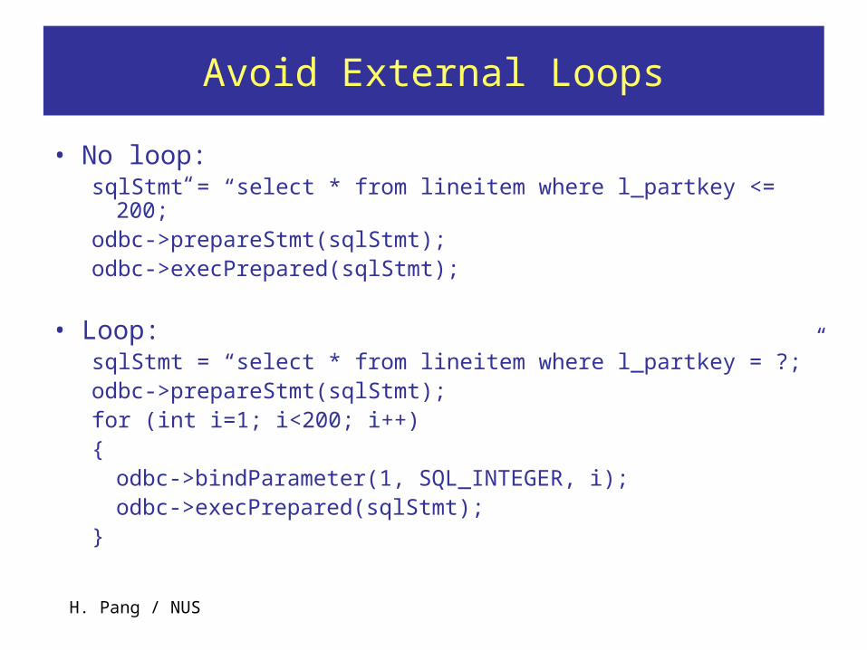
• No loop:sqlStmt = “select * from lineitem where l_partkey <=

200;”odbc->prepareStmt(sqlStmt);odbc->execPrepared(sqlStmt);

• Loop:sqlStmt = “select * from lineitem where l_partkey = ?;”odbc->prepareStmt(sqlStmt);for (int i=1; i<200; i++){

odbc->bindParameter(1, SQL_INTEGER, i);odbc->execPrepared(sqlStmt);

}

H. Pang / NUS

Avoid External Loops

• SQL Server 2000 on Windows 2000

• Crossing the application interface has a significant impact on performance

0

100

200

300

400

500

600

loop no loop

thro

ug

hp

ut

(rec

ord

s/se

c)

Let the DBMS optimizeset operations

H. Pang / NUS

Avoid Cursors

• No cursorselect * from employees;

• CursorDECLARE d_cursor CURSOR FOR select * from employees;OPEN d_cursorwhile (@@FETCH_STATUS = 0)BEGIN

FETCH NEXT from d_cursorENDCLOSE d_cursorgo

H. Pang / NUS

Avoid Cursors

• SQL Server 2000 on Windows 2000

• Response time is a few seconds with a SQL query and more than an hour iterating over a cursor

0

1000

2000

3000

4000

5000

cursor SQL

Th

rou

gh

pu

t (r

eco

rds/

sec)

H. Pang / NUS

Retrieve Needed Columns Only

– All

Select * from lineitem;

– Covered subset

Select l_orderkey, l_partkey, l_suppkey, l_shipdate, l_commitdate from lineitem;

• Avoid transferring unnecessary data

• May enable use of a covering index.

0

0.25

0.5

0.75

1

1.25

1.5

1.75

no index index

Th

rou

gh

pu

t (q

uer

ies/

mse

c)

all

covered subset

H. Pang / NUS

Use Direct Path for Bulk Loading

sqlldr directpath=true control=load_lineitem.ctl data=E:\Data\lineitem.tbl

load data infile "lineitem.tbl"into table LINEITEM appendfields terminated by '|' (

L_ORDERKEY, L_PARTKEY, L_SUPPKEY, L_LINENUMBER, L_QUANTITY, L_EXTENDEDPRICE, L_DISCOUNT, L_TAX, L_RETURNFLAG, L_LINESTATUS, L_SHIPDATE DATE "YYYY-MM-DD", L_COMMITDATE DATE "YYYY-MM-DD", L_RECEIPTDATE DATE "YYYY-MM-DD", L_SHIPINSTRUCT, L_SHIPMODE, L_COMMENT

)

H. Pang / NUS

Use Direct Path for Bulk Loading

• Direct path loading bypasses the query engine and the storage manager. It is orders of magnitude faster than for conventional bulk load (commit every 100 records) and inserts (commit for each record).

650

10000

20000

30000

40000

50000

conventional direct path insert

Th

rou

gh

pu

t (r

ec/s

ec)

H. Pang / NUS

Some Idiosyncrasies

• OR may stop the index being used– break the query and use UNION

• Order of tables may affect join implementation

H. Pang / NUS

Query Tuning – Thou Shalt …

• Avoid redundant DISTINCT• Change nested queries to join• Avoid unnecessary temp tables• Avoid complicated correlation subqueries• Join on clustering and integer attributes• Avoid HAVING when WHERE is enough• Avoid views with unnecessary joins• Maintain frequently used aggregates• Avoid external loops

H. Pang / NUS

Query Tuning – Thou Shalt …

• Avoid cursors• Retrieve needed columns only• Use direct path for bulk loading