h o, and hd16o) as obtained from ndacc/ftir solar

Earth Syst. Sci. Data, 9, 15–29, 2017www.earth-syst-sci-data.net/9/15/2017/doi:10.5194/essd-9-15-2017© Author(s) 2017. CC Attribution 3.0 License.

Tropospheric water vapour isotopologue data (H162 O,

H182 O, and HD16O) as obtained from NDACC/FTIR solar

absorption spectra

Sabine Barthlott1, Matthias Schneider1, Frank Hase1, Thomas Blumenstock1, Matthäus Kiel1,Darko Dubravica1, Omaira E. García2, Eliezer Sepúlveda2, Gizaw Mengistu Tsidu3,4, Samuel TakeleKenea3,a, Michel Grutter5, Eddy F. Plaza-Medina5, Wolfgang Stremme5, Kim Strong6, Dan Weaver6,

Mathias Palm7, Thorsten Warneke7, Justus Notholt7, Emmanuel Mahieu8, Christian Servais8,Nicholas Jones9, David W. T. Griffith9, Dan Smale10, and John Robinson10

1Institute of Meteorology and Climate Research (IMK-ASF), Karlsruhe Institute of Technology (KIT),Karlsruhe, Germany

2Izaña Atmospheric Research Center, Agencia Estatal de Meteorología (AEMET),Santa Cruz de Tenerife, Spain

3Department of Physics, Addis Ababa University, P.O. Box 1176, Addis Ababa, Ethiopia4Botswana International University of Technology and Science (BIUST) Priv. Bag 16, Palapye, Botswana

5Centro de Ciencias de la Atmósfera, Universidad Nacional Autónoma de México, 04510 Mexico City, Mexico6Department of Physics, University of Toronto, Toronto, Ontario, Canada

7Institute of Environmental Physics, University of Bremen, Bremen, Germany8Institute of Astrophysics and Geophysics, University of Liège, Liège, Belgium

9Centre for Atmospheric Chemistry, University of Wollongong, Wollongong, New South Wales, Australia10National Institute of Water and Atmospheric Research, Lauder, New Zealand

anow at: Department of Physics, Samara University, P.O. Box 132, Samara, Ethiopia

Correspondence to: Sabine Barthlott ([email protected])

Received: 11 March 2016 – Published in Earth Syst. Sci. Data Discuss.: 26 April 2016Revised: 15 November 2016 – Accepted: 21 November 2016 – Published: 20 January 2017

Abstract. We report on the ground-based FTIR (Fourier transform infrared) tropospheric water vapour iso-topologue remote sensing data that have been recently made available via the database of NDACC (Networkfor the Detection of Atmospheric Composition Change; ftp://ftp.cpc.ncep.noaa.gov/ndacc/MUSICA/) and viadoi:10.5281/zenodo.48902. Currently, data are available for 12 globally distributed stations. They have beencentrally retrieved and quality-filtered in the framework of the MUSICA project (MUlti-platform remote Sens-ing of Isotopologues for investigating the Cycle of Atmospheric water). We explain particularities of retrievingthe water vapour isotopologue state (vertical distribution of H16

2 O, H182 O, and HD16O) and reveal the need for

a new metadata template for archiving FTIR isotopologue data. We describe the format of different data com-ponents and give recommendations for correct data usage. Data are provided as two data types. The first typeis best-suited for tropospheric water vapour distribution studies disregarding different isotopologues (compari-son with radiosonde data, analyses of water vapour variability and trends, etc.). The second type is needed foranalysing moisture pathways by means of {H2O,δD}-pair distributions.

Published by Copernicus Publications.

ftp://ftp.cpc.ncep.noaa.gov/ndacc/MUSICA/

http://dx.doi.org/10.5281/zenodo.48902

16 S. Barthlott et al.: Water vapour isotopologue data from NDACC/FTIR spectra

1 Introduction

Simultaneous observations of different tropospheric waterisotopologues can provide valuable information on mois-ture source, transport, cloud processes, and precipitation (e.g.Dansgaard, 1964; Gat, 2000; Yoshimura et al., 2004). Foridentifying and analysing different tropospheric moisturepathways, the distribution of {H2O,δD} pairs (e.g. Galewskyet al., 2005; Noone, 2012; González et al., 2016) or deu-terium excess (d = δD− 8δ18; e.g. Pfahl and Sodemann,2014; Steen-Larsen et al., 2014; Aemisegger et al., 2014) areparticularly promising. The formula of deuterium excess isbased on definitions used in studies such as Craig (1961a, b)and Dansgaard (1964). The δ notation is used to express therelation of the observed isotopologue ratio to the standard ra-tio VSMOW (Vienna Standard Mean Ocean Water), where

δD= HD16O/H162 O

VSMOW − 1 and δ18=

H182 O/H16

2 OVSMOW − 1.

In recent years, there has been significant progress inmeasuring the tropospheric water vapour isotopologues; re-mote sensing observations are particularly interesting sincethey can provide data for the free troposphere and they canbe performed continuously (for cloud-free conditions). Dur-ing MUSICA (MUlti-platform remote Sensing of Isotopo-logues for investigating the Cycle of Atmospheric water),a method has been developed to obtain tropospheric watervapour profiles as well as {H2O,δD} pairs from ground-based FTIR (Fourier transform infrared) and space-basedIASI (Infrared Atmospheric Sounding Interferometer) ob-servations. The ground-based FTIR spectra are measuredin the framework of the NDACC (Network for the Detec-tion of Atmospheric Composition Change, www.ndacc.org).These spectra are of very high quality and have been avail-able at some stations since the 1990s, thus offering long-term data records, which are of particular interest to cli-matological studies or for assessing the stability of long-term satellite data records. Network-wide consistent qualityof the MUSICA NDACC/FTIR water vapour isotopologuedata is ensured by central data processing and quality con-trol (e.g. all data are quality-filtered by the XCO2 method aspresented in Barthlott et al., 2015). The high quality of theMUSICA ground- and space-based remote sensing data hasbeen demonstrated by empirical validation studies (Schnei-der et al., 2016).

In this paper, we present the MUSICA NDACC/FTIRdata as provided recently via the NDACC database (see alsoBarthlott et al., 2016). Our objective is to make a data useraware of the nature of the data and to give recommendationsand explanations for correct data usage. Section 2 briefly de-scribes the particularity of retrievals of the water vapour iso-topologue state. It is shown that for achieving an optimal es-timation of the tropospheric water vapour isotopologue state,we have to work with full state vectors consisting of differentisotopologues, i.e. a state vector consisting of several tracegases. As a result, water vapour isotopologue data cannot be

provided in exactly the same data format as other FTIR data.In Sect. 3 we describe the data format used for providing thisnew data via the NDACC database. Section 4 gives some in-sight into the data characteristics and recommendation forworking with this new data set. In Sect. 6, we conclude andsummarise our results. The summarised guidelines for cor-rect data usage can be found in Table 3.

2 Optimal estimation of the water vapourisotopologue state

2.1 The principle of optimal estimation retrieval methods

Atmospheric remote sensing retrievals characterise an atmo-spheric state from a measured spectrum. However, such aninversion problem is often ill-posed (a lot of different atmo-spheric states can explain the measured spectrum). Conse-quently, for solving this problem, some kind of regularisa-tion is required. This can be introduced by means of a costfunction:[y−F (x,p)

]T S−1ε

[y−F (x,p)

]+ [x− xa]T S−1

a [x− xa] . (1)

Here, the first term is a measure of the difference betweenthe measured spectrum (y) and the spectrum simulated for agiven atmospheric state (x), where F represents the forwardmodel, which simulates a spectrum y for a given state x, tak-ing into account the actual measurement noise level (Sε is themeasurement noise covariance). Vector p represents auxil-iary atmospheric parameters (like temperature) or instrumen-tal characteristics (like the instrumental line shape). The sec-ond term of the cost function (1) is the regularisation term.It constrains the atmospheric solution state (x) towards an apriori most likely state (xa), where kind and strength of theconstraint are defined by the a priori covariance matrix Sa.The constrained solution is reached at the minimum of thecost function (1). This method of updating the knowledgeabout the a priori state with information from a measurementis known as the optimal estimation method, which is a stan-dard remote sensing retrieval method (see Rodgers, 2000, formore details) in which validity of the optimal estimation so-lution strongly depends on a correct and comprehensive de-scription of the a priori state by means of xa and Sa. For read-ers that are not familiar with remote sensing mathematics, weadded some mathematical foundations in Appendix A.

2.2 Correct description of the water vapourisotopologue state

Water vapour isotopologues with reasonably strong and well-discernible spectral infrared signatures are H16

2 O, H182 O, and

HD16O. Hereafter, we will refer to the combined states ofH16

2 O, H182 O, and HD16O as the full water vapour isotopo-

logue state.

Earth Syst. Sci. Data, 9, 15–29, 2017 www.earth-syst-sci-data.net/9/15/2017/

www.ndacc.org


S. Barthlott et al.: Water vapour isotopologue data from NDACC/FTIR spectra 17

Tropospheric water vapour shows a strong variation (inspace and time) and it can be better described by a log-normal than by a normal distribution (Hase et al., 2004;Schneider et al., 2006). Furthermore, the different isotopo-logues vary mostly in equal measure, i.e. their variationsare strongly correlated and the variation in the isotopo-logue ratios is much smaller. For instance, the variationin ln

[HD16O

]− ln

[H16

2 O]

is about 1 order of magnitudesmaller and the variations in ln

[H18

2 O]− ln

[H16

2 O]

is about2 orders of magnitude smaller than the correlated variationsin ln

[H16

2 O], ln[H18

2 O], and ln

[HD16O

](Craig and Gordon,

1965). An elegant method for correctly describing the natureof the full water vapour isotopologue state is to work on alogarithmic scale (due to the log-normal distribution charac-teristic) and with the following three states:

– the humidity-proxy state:

humidity=13

(ln[H16

2 O]+ ln

[H18

2 O]+ ln

[HD16O

]); (2)

– the δD-proxy state:

δD= ln[HD16O

]− ln

[H16

2 O]; (3)

– the deuterium-excess proxy state (d-proxy state):

d = ln[HD16O

]− ln

[H16

2 O]

− 8(

ln[H18

2 O]− ln

[H16

2 O]). (4)

The water vapour isotopologue state can be expressed onthe basis of

{ln[H16

2 O], ln[H18

2 O], ln[HD16O

]}or on the

basis of the proxies of {humidity,δD,d}. Both expressionsare equivalent. Each basis has the dimension nol× 3, wherenol is the number of levels of the radiative transfer modelatmosphere and three different combinations of the threedifferent isotopologues have to be considered. In the fol-lowing, the full water vapour isotopologue state vector ex-pressed on the

{ln[H16

2 O], ln[H18

2 O], ln[HD16O

]}basis and

the {humidity,δD,d}-proxy basis will be referred to as xl

and xl′, respectively, where index “l” stands for logarithmicscale. A basis transformation can be achieved by operator P:

P=

131

131

131

−1 0 1

71 −81 1

. (5)

Here, the nine matrix blocks have the dimension nol× nol, 1stands for an identity matrix, and the state vectors xl and xl′

are related by

xl′= Pxl. (6)

Similarly, covariance matrices can be expressed in the twobasis systems and the respective matrices Sl, and Sl′ are re-lated by

Sl′= PSlPT . (7)

The variation in humidity, δD, and deuterium excess havedifferent magnitudes. This can be well considered by givingthe a priori covariance matrix in the {humidity,δD,d}-proxybasis:

Sla′=

Slahum

0 00 Sl

aδD 00 0 Sl

ad

. (8)

This assumes that humidity, δD, and deuterium excessvary independently, which is actually not the case in thelower/middle troposphere. However, the correlation betweenhumidity, δD, and deuterium excess is a detail. It is impor-tant that the different magnitudes of variability are taken intoaccount (the entries of Sl

ahumare much larger than the entries

of SlaδD and Sl

ad ).The covariance matrix Sl

a can be calculated as (accordingto Eq. 7)

Sla = P−1Sl

a′P−T

=

1 −381

1241

1 −141 −

1121

1 581

1241

Slahum

0 00 Sl

aδD 00 0 Sl

ad

1 1 1

−381 −

141

581

1241 −

1121

1241

=

Slahum+

982 Sl

aδD +1

242 Slad Sl

ahum+

682 Sl

aδD −2

242 Slad

Slahum+

682 Sl

aδD −2

242 Slad Sl

ahum+

482 Sl

aδD +4

242 Slad

Slahum−

1582 Sl

aδD +1

242 Slad Sl

ahum−

1082 Sl

aδD −2

242 Slad

Slahum−

1582 Sl

aδD +1

242 Slad

Slahum−

1082 Sl

aδD −2

242 Slad

Slahum+

2582 Sl

aδD +1

242 Slad

. (9)

This matrix Sla correctly captures the covariance of the a pri-

ori state in the{ln[H16

2 O], ln[H18

2 O], ln[HD16O

]}basis and

it is important for a correct formulation of the cost func-tion (1) and thus for setting up a correctly constrained op-timal estimation retrieval of the water vapour isotopologuestate.

Matrix Sla reveals the complex covariances between the

state vector components of xl, in which it has to be consid-ered that the entries of Sl

ahumare much larger than the en-

tries of SlaδD and significantly larger than the entries of Sl

ad ,which means that the nine nol× nol blocks of Sl

a have almostthe same entries. The variations in ln

[H16

2 O], ln[H18

2 O], and

ln[HD16O

]are strongly correlated and we cannot work with

individual state vectors that report the states of the differ-ent isotopologues independently. Instead, we have to de-scribe the full isotopologue state by a single state vectorwith the dimension nol× 3. This is the reason why MUSICANDACC/FTIR water vapour isotopologue data cannot beprovided in the same data format as other NDACC/FTIR

www.earth-syst-sci-data.net/9/15/2017/ Earth Syst. Sci. Data, 9, 15–29, 2017


data. A slightly extended data format is needed, which is de-scribed in the next section.

2.3 The MUSICA (v2015) ground-based NDACC/FTIRretrieval setup

In Schneider et al. (2012), the MUSICA NDACC/FTIR re-trieval setup, such as interfering gases and temperature fit, isdescribed in great detail. Here, we focus on the modificationmade for the retrieval version (v2015).

For the previous retrieval version, we used 11 spectral win-dows with lines of water vapour isotopologues (see Fig. 2 ofSchneider et al., 2012). For the final MUSICA retrieval ver-sion (v2015), we removed windows with strong H16

2 O linesand replaced them by windows with weaker lines. By thismodification, we want to make sure that even for very humidsites observed spectral lines do not saturate. Furthermore, weadd a second window where a H18

2 O signature dominates.The nine spectral water vapour isotopologue windows aredepicted in Fig. 1 for an observation and fit, which are typi-cal for the different NDACC stations. In addition, we fit thethree spectral windows with the CO2 lines, which is bene-ficial for atmospheric temperature retrievals (the CO2 linesare the same as for the previous retrieval version: between2610.35 and 2610.8, 2613.7 and 2615.4, and 2626.3 and2627.0 cm−1; not shown). All of these spectral windows areobserved within NDACC filter #3.

For v2015, we perform an optimal estimation of the{humidity,δD,d}-proxy states as explained in Sect. 2.2.This is a further development of the previous retrievalversion (there the optimal estimation was made for the{humidity,δD}-proxy states; Sects. 3 and 4 of Schneideret al., 2012). Consistent with the previous version, we per-form simultaneous but individual fits (no cross-constraints)for profiles of the water vapour isotopologue H17

2 O, temper-ature, and interfering species CO2, O3, N2O, CH4, and HCl.

For the previous version, we used HITRAN 2008 line pa-rameters (Rothman et al., 2009), whereas for v2015 we workwith HITRAN 2012 parameters (Rothman et al., 2013). Forboth versions, the water vapour isotopologues parametershave been adjusted for the speed-dependent Voigt line shape(Schneider et al., 2011). For further optimisation of the HI-TRAN parameters, we used high-quality H2O and δD air-craft in situ profile references, coincident FTIR spectra, andFTIR spectra measured at three rather distinct sites (Izaña onTenerife, subtropical ocean; Karlsruhe, central Europe; andKiruna, northern Sweden). This method for line parameteroptimisation by means of atmospheric spectra is describedin detail in Schneider and Hase (2009) and Schneider et al.(2011). We changed line intensities and broadening parame-ters by about 5–10 %, which is in agreement with the uncer-tainty values as given in the HITRAN parameter files. Moredetails on the modification of the line parameters as shownin Fig. 1 are given in Appendix B.

The empirical assessment study of Schneider et al.(2016) suggests an accuracy for the MUSICA (v2015)NDACC/FTIR H2O and δD products of about 10 % and10 ‰, respectively.

3 Data set description

MUSICA NDACC/FTIR water vapour isotopologue dataare available via the NDACC database and can be ac-cessed via ftp://ftp.cpc.ncep.noaa.gov/ndacc/MUSICA/ andvia doi:10.5281/zenodo.48902. The data are provided asHDF4 files and they have been generated in compliance withGEOMS (Generic Earth Observation Metadata Standard).

For isotopologue data, a new metadata template, GEOMS-TE-FTIR-ISO-001, has been set up. It is almost identi-cal to the GEOMS-TE-FTIR template (used for all otherFTIR data provided via NDACC in HDF4 format) buthas the additional variable “CROSSCORRELATE.N”. ForMUSICA data, this new variable has three entries: “H16

2 O”,“H18

2 O”, and “HD16O”. This enables the three trace gasesH16

2 O, H182 O, and HD16O to be provided as one full state

vector (vector with nol× 3 elements) together with theirfull averaging kernels and full error covariances (both of(nol× 3)× (nol× 3) dimension) in one data file. To be com-pliant with GEOMS, the data are provided on a linear scale(and not on a logarithmic scale on which the inversion is per-formed; see Sect. 2).

All the isotopologue data have been normalised with re-spect to their natural isotopologue abundances. These natu-ral abundances are 0.997317 for H16

2 O, 0.002000 for H182 O,

and 3.106930× 10−4 for HD16O. This normalisation means

that δD can directly be calculated as( [

HD16O][

H162 O

] − 1)

from

provided H162 O, H18

2 O, and HD16O amounts. Similarly, deu-

terium excess can be calculated as( [

HD16O][

H162 O

] − 1)− 8×( [

H182 O

][H16

2 O] − 1

).

Two different data types are provided. The first type isstored in HDF files called “ftir.iso.h2o”. These files report thebest estimate of the H16

2 O state, but its usefulness for isotopo-logue studies (e.g. in the context of {H2O,δD}-distributionplots) is significantly compromised. The second type isstored in HDF files called “ftir.iso.post.h2o”. This data typeshould be used for analysing {H2O,δD}-distribution plots.Section 4 gives more details on the different data types.

The number of stations contributing to the MUSICANDACC/FTIR data set is gradually increasing and Table 1gives an overview of the current status (status for January2016) together with mean DOFS (degrees of freedom of sig-nal) for the two data types. The stations are well distributedfrom the Arctic to the Antarctic and in some cases offer datafrom the late 1990s onward. A further extension of this dataset to other sites or for some stations to measurements made





R

M

MS

W

Figure 1. The spectral windows used for the MUSICA ground-based NDACC/FTIR retrievals. Shown is an example of a typical measure-ment (Karlsruhe, 15 September 2011, 12:03 UT; solar elevation: 43.1◦; H2O slant column: 22.9 mm). Black line: measurement; red line:simulation; blue line: residual (difference between measurement and simulation).

Table 1. List of current MUSICA NDACC/FTIR sites (ordered from north to south) and available MUSICA data record. DOFS (type 1)reports the typical trace of Al

H2O and DOFS (type 2) that of Al∗11 ≈ Al∗

22 for optimal estimation of {H2O,δD} pairs (example kernel plotted inFig. 5).

Site Location Altitude Data record DOFS (type 1) DOFS (type 2)

Eureka, Canada 80.1◦ N, 86.4◦W 610 m a.s.l. 2006–2014 2.9 1.7Ny-Ålesund, Norway 78.9◦ N, 11.9◦ E 21 m a.s.l. 2005–2014 2.8 1.6Kiruna, Sweden 67.8◦ N, 20.4◦ E 419 m a.s.l. 1996–2014 2.8 1.6Bremen, Germany 53.1◦ N, 8.9◦ E 27 m a.s.l. 2004–2014 2.8 1.6Karlsruhe, Germany 49.1◦ N, 8.4◦ E 110 m a.s.l. 2010–2014 2.8 1.6Jungfraujoch, Switzerland 46.6◦ N, 8.0◦ E 3580 m a.s.l. 1996–2014 2.7 1.6Izaña, Tenerife, Spain 28.3◦ N, 16.5◦W 2367 m a.s.l. 1999–2014 2.9 1.7Altzomoni, Mexico 19.1◦ N, 98.7◦W 3985 m a.s.l. 2012–2014 2.7 1.7Addis Ababa, Ethiopia 9.0◦ N, 38.8◦ E 2443 m a.s.l. 2009–2013 2.6 1.6Wollongong, Australia 34.5◦ S, 150.9◦ E 30 m a.s.l. 2007–2014 2.7 1.6Lauder, New Zealand 45.1◦ S, 169.7◦ E 370 m a.s.l. 1997–2014 2.8 1.6Arrival Heights, Antarctica 77.8◦ S, 166.7◦ E 250 m a.s.l. 2002–2014 2.7 1.4

in the beginning of the 1990s is feasible but was not possiblewithin the MUSICA project.

3.1 Averaging kernels

An averaging kernel describes how a retrieved state vec-tor responds to variations in the real atmospheric state vec-tor. The MUSICA NDACC/FTIR isotopologue state vectorconsists of three trace gases and the corresponding full av-eraging kernel matrix A consists of nine blocks, each ofwhich is a nol× nol matrix. In total, A has the dimension(nol× 3)× (nol× 3):

A=

A11 A12 A13A21 A22 A23A31 A32 A33

. (10)

The three blocks along the diagonal describe the direct re-sponses: block A11 for the response of the H16

2 O retrievalproduct to real atmospheric H16

2 O variations, block A22 forthe response of the H18

2 O retrieval product to real atmo-spheric H18

2 O variations, and block A33 for the response

of the HD16O retrieval product to real atmospheric HD16Ovariations. The outer diagonal blocks describe the cross re-sponses: two blocks for the response of the H16

2 O retrievalproduct to real atmospheric H18

2 O and HD16O variations(A12 and A13, respectively), two blocks for the responseof the H18

2 O retrieval product to real atmospheric H162 O

and HD16O variations (A21 and A23, respectively), and twoblocks for the response of the HD16O retrieval product toreal atmospheric H16

2 O and H182 O variations (A31 and A32, re-

spectively). The different blocks of the matrix (see Fig. 2) canbe easily identified by the values of the variable “CROSS-CORRELATE.N”: 1= H16

2 O, 2= H182 O, and 3= HD16O.

3.2 Error covariances

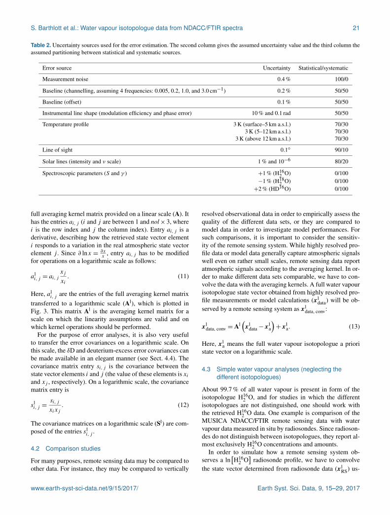
For error calculations, the same uncertainty sources areassumed for all MUSICA NDACC/FTIR stations and aregrouped into statistical and systematic errors. An overviewof the uncertainty assumptions is given in Table 2. Error co-variances for each of these uncertainty sources are calculatedaccording to Rodgers (2000). Total error covariances are ob-



A

L –1

Figure 2. Column entries of the nine blocks of the full averaging kernel matrix A (see Eq. 10). Shown are some columns of the kernel matrixfor 0.5 km (black), 2.4 km (red), 4.9 km (green), 8.0 km (blue), and 13.6 km (light blue). This kernel is for the retrieval with the spectrum andfit as shown in Fig. 1.

tained as the sum of the individual error covariances, cal-culated separately for statistical and systematic errors. Fullerror covariance matrices have the same matrix dimensionas the full averaging kernel matrix and provide informationabout the errors and how the errors between different alti-tudes as well as between the three different isotopologuesare correlated.

3.3 Column densities

Partial and total column densities are also provided as wellas column sensitivity averaging kernels and column error co-variances. Partial columns are calculated for the layers be-tween the nol atmospheric levels. A full water vapour iso-topologue partial column state vector has (nol− 1)× 3 el-ements (i.e. nol−1 elements for each of the three isotopo-logues). The column sensitivity averaging kernel has the di-mension ((nol− 1)× 3)× 3 and describes the sensitivities ofthe total column retrieval product (columns of H16

2 O, H182 O,

and HD16O) with respect to real atmospheric variations in theisotopologues’ partial columns. Column error covariancesare provided for statistical and systematic errors indepen-dently and are matrices with the dimension 3× 3. They de-scribe total column errors for the three isotopologues andhow these errors are correlated.

All column data are calculated from mixing ratio data(mixing ratio state vector, error covariances, and averagingkernels). For a conversion of mixing ratios (ppmv) to num-ber densities (molec.cm−3), we use the ideal gas law and

work with retrieved temperature profiles. Temperature andpressure profiles are also provided in the HDF files.

Please note: since GEOMS requires the same number ofelements of column data and the respective mixing ratio data,value 0 has been added for all column data values at level nol.

4 Recommendations for data usage

In order to be compliant with GEOMS, data are providedfor the full state vector consisting of the H16

2 O, H182 O, and

HD16O state vectors and in mixing ratios (ppmv). How-ever, actually the MUSICA NDACC/FTIR retrieval workson a logarithmic scale and performs an optimal estimationof combined isotopologue states (see Sect. 2). These detailshave to be considered when working with these data.

4.1 Transfer to a logarithmic scale

For operations with averaging kernels (e.g. when adjustingmodel data to the sensitivity of a remote sensing system), ithas to be considered that the retrieval works on a logarith-mic scale, because only on this scale are linearity assump-tions valid. Therefore, it is strongly recommended to transferthe averaging kernels to a logarithmic scale; in doing so, ithas to be considered that the derivatives are calculated forthe state as given by the retrieval state vector x. The full re-trieval state vector consists of the retrieved H16

2 O, H182 O, and

HD16O states, i.e. it is a vector with nol× 3 elements xi (withi between 1 and nol× 3). The full averaging kernel matrixhas the dimension (nol× 3)× (nol× 3). Figure 2 plots the



Table 2. Uncertainty sources used for the error estimation. The second column gives the assumed uncertainty value and the third column theassumed partitioning between statistical and systematic sources.

Error source Uncertainty Statistical/systematic

Measurement noise 0.4 % 100/0

Baseline (channelling, assuming 4 frequencies: 0.005, 0.2, 1.0, and 3.0 cm−1) 0.2 % 50/50

Baseline (offset) 0.1 % 50/50

Instrumental line shape (modulation efficiency and phase error) 10 % and 0.1 rad 50/50

Temperature profile 3 K (surface–5 km a.s.l.) 70/303 K (5–12 km a.s.l.) 70/30

3 K (above 12 km a.s.l.) 70/30

Line of sight 0.1◦ 90/10

Solar lines (intensity and ν scale) 1 % and 10−6 80/20

Spectroscopic parameters (S and γ ) +1 % (H162 O) 0/100

−1 % (H182 O) 0/100

+2 % (HD16O) 0/100

full averaging kernel matrix provided on a linear scale (A). Ithas the entries ai, j (i and j are between 1 and nol× 3, wherei is the row index and j the column index). Entry ai, j is aderivative, describing how the retrieved state vector elementi responds to a variation in the real atmospheric state vectorelement j . Since ∂ lnx = ∂x

x, entry ai, j has to be modified

for operations on a logarithmic scale as follows:

ali, j = ai, j

xj

xi. (11)

Here, ali, j are the entries of the full averaging kernel matrix

transferred to a logarithmic scale (Al), which is plotted inFig. 3. This matrix Al is the averaging kernel matrix for ascale on which the linearity assumptions are valid and onwhich kernel operations should be performed.

For the purpose of error analyses, it is also very usefulto transfer the error covariances on a logarithmic scale. Onthis scale, the δD and deuterium-excess error covariances canbe made available in an elegant manner (see Sect. 4.4). Thecovariance matrix entry si, j is the covariance between thestate vector elements i and j (the value of these elements is xiand xj , respectively). On a logarithmic scale, the covariancematrix entry is

sli, j =

si, j

xixj. (12)

The covariance matrices on a logarithmic scale (Sl) are com-posed of the entries sl

i, j .

4.2 Comparison studies

For many purposes, remote sensing data may be compared toother data. For instance, they may be compared to vertically

resolved observational data in order to empirically assess thequality of the different data sets, or they are compared tomodel data in order to investigate model performances. Forsuch comparisons, it is important to consider the sensitiv-ity of the remote sensing system. While highly resolved pro-file data or model data generally capture atmospheric signalswell even on rather small scales, remote sensing data reportatmospheric signals according to the averaging kernel. In or-der to make different data sets comparable, we have to con-volve the data with the averaging kernels. A full water vapourisotopologue state vector obtained from highly resolved pro-file measurements or model calculations (xl

data) will be ob-served by a remote sensing system as xl

data, conv:

xldata, conv = Al

(xl

data− xla

)+ xl

a. (13)

Here, xla means the full water vapour isotopologue a priori

state vector on a logarithmic scale.

4.3 Simple water vapour analyses (neglecting thedifferent isotopologues)

About 99.7 % of all water vapour is present in form of theisotopologue H16

2 O, and for studies in which the differentisotopologues are not distinguished, one should work withthe retrieved H16

2 O data. One example is comparison of theMUSICA NDACC/FTIR remote sensing data with watervapour data measured in situ by radiosondes. Since radioson-des do not distinguish between isotopologues, they report al-most exclusively H16

2 O concentrations and amounts.In order to simulate how a remote sensing system ob-

serves a ln[H16

2 O]

radiosonde profile, we have to convolvethe state vector determined from radiosonde data (xl

RS) us-



A

L

Figure 3. Same as Fig. 2 but for the logarithmic-scale kernel matrix Al.

ing the averaging kernel blocks Al11, Al

12, and Al13 (these

blocks are depicted in Fig. 3). The radiosonde only measuresln[H16

2 O]; it does not measure ln

[H18

2 O]

and ln[HD16O

].

However, ln[H18

2 O]

and ln[HD16O

]are strongly correlated

with ln[H16

2 O]:

ln[H18

2 O]− ln

[H18

2 O]

a= ln

[H16

2 O]− ln

[H16

2 O]

a

+18{δD− δDa− (d − da)} , (14)

and

ln[HD16O

]− ln

[HD16O

]a= ln

[H16

2 O]− ln

[H16

2 O]

a

+{δD− δDa} (15)

(see Eqs. 3 and 4). Here, index a identifies a priori data. Likeall full isotopologue state vectors, xl

RS has nol× 3 compo-nents. The first section of nol components is determined bythe in situ measured ln

[H16

2 O]

profile. The second section ofnol components is also determined by the in situ measuredln[H16

2 O]

profile, but we have to consider an uncertainty ofthese vector components according to the uncertainty covari-ance matrix 1

82 (SlaδD +Sl

ad ) (see Eq. 14). The uncertainty isdue to the fact that a radiosonde does not measure H18

2 O.The third section of nol components is similarly determinedby the in situ measured ln

[H16

2 O]

profile, but with an un-certainty according to the uncertainty covariance matrix Sl

aδD(see Eq. 15), in which the uncertainty is caused by miss-ing HD16O radiosonde measurements. Hence, a ln

[H16

2 O]

radiosonde profile is equivalent to a ln[H16

2 O]

remote sens-

ing observation of(Al

11+Al12+Al

13

)(xl

RS− xla

)+ xl

a, (16)

in which there is an uncertainty in the equivalency of

182 Al

12

(Sl

aδD +Slad

)Al

12T+Al

13SlaδDAl

13T, (17)

which is due to missing radiosonde observations of H182 O and

HD16O.Equation 16 reveals that the nol× nol averaging kernel

matrix AlH2O = Al

11+Al12+Al

13 is a good proxy for the re-mote sensing system’s sensitivity with respect to H16

2 O andthus water vapour in general (about 99.7 % of all watervapour molecules are H16

2 O isotopologues). The columns ofthe matrix Al

H2O are plotted in Fig. 4.

4.4 Utility of the {humidity,δD,d }-proxy basis and dataa posteriori processing

The MUSICA NDACC/FTIR retrieval performs an optimalestimation of the humidity, δD, and deuterium-excess proxystates. Although optimal estimation of these states is madein a single retrieval process, it is made for each of the threestates independently, meaning, for instance, that the estima-tion is not optimal for the {H2O,δD} pairs. The reason is thatthe remote sensing system’s sensitivity for the humidity stateis much higher than for the δD-state (and significantly higherthan for the deuterium-excess state). The problem becomesclearly visible by transforming the full averaging kernel ma-trix onto the {humidity,δD,d}-proxy basis:

Al′= PAlP−1. (18)



A

L

Figure 4. Logarithmic-scale kernel matrix AlH2O = Al

11+Al12+

Al13, with the Al blocks as plotted in Fig. 3.

Here, Al′ is the full averaging kernel matrix in the{humidity,δD,d}-proxy basis. It is depicted in Fig. 5, whichclearly reveals larger sensitivity for humidity (kernel blockAl

11′) than for δD (kernel block Al

22′). Data with this charac-

teristic cannot be used in the context of {H2O,δD}-pair dis-tribution analyses.

A transformation of the error covariance matrices onto the{humidity,δD,d}-proxy basis (for transformation operation,see Eq. 7) is very helpful for analysing the error characteris-tics of the H2O, δD, and deuterium-excess data because errorcovariances expressed in the {humidity,δD,d}-proxy basisare good proxies for the error covariances of H2O, δD, anddeuterium excess (for more details see discusion in Sect. 4.2of Schneider et al., 2012).

4.4.1 A posteriori processing for a quasi-optimalestimation of

{H2O,δD

}pairs

During MUSICA, an a posteriori processing method forobtaining a quasi-optimal estimation product of {H2O,δD}pairs has been developed. The a posteriori processing bringsabout a moderate reduction in the H2O sensitivity and in theδD cross dependencies on H2O (Sect. 4.2 in Schneider et al.,2012). The operation has to be performed with logarithmic-scale full state vector, averaging kernel matrix, and covari-ance matrices (xl, Al and Sl):

xl∗= P−1CP(xl

− xla)+ xl

a, (19)

Al∗= P−1CPAl, (20)

and

Sl∗= P−1CPSlPTCT P−T . (21)

Here, xl∗, Al∗, and Sl∗ are a posteriori-processedlogarithmic-scale full state vector, averaging kernelmatrix, and covariance matrices, respectively. Operator P is

introduced by Eq. (5) and the a posteriori operator C is

C=

Al22′ 0 0

−Al21′

1 00 0 1

. (22)

Figure 6 depicts the a posteriori processed averaging ker-nel Al∗. It is obvious that the processing ensures that the sen-sitivity for humidity (kernel block Al∗

11) and for δD (kernelblock Al∗

22) are almost identical. Data with this characteristicare provided on a linear scale in the “ftir.iso.post.h2o” HDFfiles and they are well suited for {H2O,δD}-pair distributionanalyses.

4.4.2 A posteriori processing for a quasi-optimalestimation of

{H2O,δD,d

}triplets

Figure 6 reveals that kernel block Al∗33 is still rather differ-

ent from the kernel blocks Al∗11 and Al∗

22. Furthermore, thereis a rather large cross dependency of δD on deuterium ex-cess (kernel block Al∗

32). This means that a posteriori correc-tion with operator C according to Eq. (22) is not sufficientfor providing deuterium excess data that can be analysed to-gether with H2O and δD and that is of sufficient quality. Forsuch purpose, the a posteriori treatment has to be stronger,which can be achieved by using the following operator C:

C=

Al33′ 0 0

−Al21′ Al

33′ 0

−Al31′−Al

32′

1

. (23)

Figure 7 depicts the a posteriori processed averaging ker-nel Al∗ by using C from Eq. (23). This treatment ensuresthat the three blocks Al∗

11, Al∗22, and Al∗

33 are almost identical.Nevertheless, the retrieved deuterium excess shows still somecross dependency on δD (averaging kernel block Al∗

32). Cur-rently, these data are not provided via the NDACC database,mainly because it has so far not been possible to empiricallyprove the quality of this deuterium-excess remote sensingdata. In any case, interested users are welcome to investigatethe quality of these data. The required a posteriori processingcan be made by using the data provided in “ftir.iso.h2o” HDFfiles and by following the description given in this paper (ifunclear, please contact the MUSICA team).

5 Data availability

The MUSICA NDACC/FTIR data are publicly available viathe database of NDACC (ftp://ftp.cpc.ncep.noaa.gov/ndacc/MUSICA/) and via doi:10.5281/zenodo.48902 (Barthlott etal., 2016).






A

L

Figure 5. Column entries of the nine blocks of the logarithmic-scale kernel matrix in the {humidity,δD,d}-proxy state (Al′; see Eq. 18).

A

L

Figure 6. Same as Fig. 5 but after a posteriori processing with C from Eq. 22 (Al∗; see Eq. 20).

6 Conclusions

For a correct optimal estimation retrieval of the full wa-ter vapour isotopologue state, we have to consider that at-mospheric variations in different isotopologues are stronglycorrelated. This strong correlation is then also present inthe retrieved state vectors and it has to be considered wheninterpreting averaging kernels and error covariances. As aconsequence, it makes little sense to provide different iso-topologues in the form of individual states and via individ-ual data sets. Instead, it is essential that water vapour iso-

topologues are made available as single full state vectorstogether with their full averaging kernels and error covari-ances. The standard GEOMS metadata template for FTIRdata on the NDACC database (called GEOMS-TE-FTIR)does not allow data to be provided in such a format anda slight extension of the standard FTIR template has beenmade (the modified template is called GEOMS-TE-FTIR-ISO-001). The MUSICA NDACC/FTIR data are now avail-able in this new data format on the NDACC database and viadoi:10.5281/zenodo.48902. The extended template can also





A

L

Figure 7. Same as Fig. 6 but using C from Eq. 23.

Table 3. Summary of recommendations and comments for the two principal types of data users.

User type HDF file Recommendations and comments

H2O profiles ftir.iso.h2o transfer data onto a logarithmic scale (see Sect. 4.1)use H16

2 O retrieval products as H2O (more than 99.7 % of all water vapour is in form of H162 O)

use averaging kernel AlH2O = Al

11+Al12+Al

13 (see Sect. 4.3)

{H2O,δD} pairs ftir.iso.post.h2o comment: all “ftir.iso.post.h2o” retrieval products are corrected as described in Sect. 4.4.1transfer data onto a logarithmic scale (see Sect. 4.1)use data in the {humidity,δD,d}-proxy basis for sensitivity and error assessments (see Sect. 4.4)

be used for providing isotopologue data of other molecules(e.g. ozone isotopologue data).

In order to be compliant with GEOMS, the data are pro-vided on a linear scale and as volume mixing ratio (ppmv).However, since the retrieval is performed on a logarithmicscale, it is recommended to transfer states, kernels, and av-eraging kernels onto a logarithmic scale. On this scale, lin-earity in the context of averaging kernel operations can beassumed and we can furthermore make transformations be-tween the

{ln[H16

2 O], ln[H18

2 O], ln[HD16O

]}basis and the

{humidity,δD,d}-proxy basis. The transformation of statevector, error covariances and averaging kernels onto the{humidity,δD,d}-proxy basis gives insight into the actualsensitivity and error characteristics of the retrieved humid-ity, δD, and deuterium-excess values. It can be shown that{H2O,δD}-data pairs can be obtained in an optimal estima-tion sense, but only if the retrieval output undergoes a poste-riori processing. Error estimations are discussed in detail inSchneider et al. (2012). The leading random error source isuncertainty in the atmospheric temperature profiles and arte-facts in the spectral baseline (like channelling or offset). Sys-

tematic errors are dominated by uncertainties in the spectro-scopic parameters. There are inconsistencies between param-eters for different lines as well as inadequacies in the lineshape model used. To determine the importance of the dif-ferent aspects for improving the accuracy, further dedicatedresearch projects would be needed.

The MUSICA NDACC/FTIR data are made availablein the form of two different data types. The first type(“ftir.iso.h2o”) is the direct retrieval output. It reports theoptimal estimations of the states ln

[H16

2 O], ln

[H18

2 O],

and ln[HD16O

], and a user should work with these data

for studies that focus on water vapour and disregard thedifference between the isotopologues. The second type(“ftir.iso.post.h2o”) is the a posteriori processed output. Itreports the optimal estimation of {H2O,δD} pairs and itshould be used for analysing moisture pathways by means of{H2O,δD}-distribution plots. Table 3 summarises the guide-lines that should be considered for correct data usage.



Appendix A: Mathematical foundations ofatmospheric remote sensing

Atmospheric remote sensing means that the atmosphericstate is retrieved from the radiation measured after having in-teracted with the atmosphere. For a mathematical treatment,vectors are used for describing the atmospheric state and themeasured radiation. Hence, vector and matrix algebra is thetool used in the context of remote sensing retrievals and re-mote sensing product characterisation. In the following, webriefly explain the connections between vector and matrixalgebra and atmospheric remote sensing that are relevant forour paper. For a more detailed introduction, please refer toRodgers (2000). For a general introduction to vector and ma-trix algebra, dedicated textbooks should be consulted (e.g.Herstein and Winter, 1988; Strang, 2016).

A1 Atmospheric state vector and measurement vector(x and y):

We are interested in the vertical distribution of H162 O, H18

2 O,and HD16O and our atmospheric state is a vector whosecomponents represent the H16

2 O, H182 O, and HD16O concen-

trations at different atmospheric altitudes. The atmosphericstate vector is generally written as x. Our measurementsare high-resolution infrared spectra and the different spec-tral bins of a measured spectrum are represented by the com-ponents of the measurement vector. This vector is generallywritten as y.

A2 A priori state vector and covariance matrix (xa andSa)

The interaction of radiation with the atmosphere is modelledby a radiative transport model (also called a forward model,F ) and allows relating the measurement vector and the atmo-spheric state vector by

y = F (x). (A1)

We measure y and are interested in x. However, a direct in-version of Eq. (A1) is generally not possible, because thereare many atmospheric states x that can explain one and thesame measurement y. This means we face an ill-posed prob-lem and for the inversion we need an additional constraintor regularisation. This leads us to the optimal estimationmethod. For this method we set up a cost function that com-bines the information provided by the measurement with apriori known characteristics of the atmospheric state (seeEq. 1 in Sect. 2.1). This a priori knowledge about the atmo-spheric state is collected as the mean and covariances in formof the a priori state vector (xa) and the a priori covariance ma-trix (Sa). By minimising the cost function (Eq. 1), we get themost probable atmospheric state for the given measurement,i.e. the optimally estimated atmospheric state.

A3 Averaging kernel matrix (A)

The averaging kernel relates the real atmospheric state to theatmospheric state as provided by the remote sensing retrieval(see, for instance, Eq. 13). The averaging kernel matrix el-ement (i, j , i.e. element in line i and column j of the ma-trix) reveals how a change in the real atmospheric state vec-tor component j will affect the retrieved atmospheric statevector component i. The averaging kernel is an importantcomponent of a remote sensing retrieval and it is calculatedby the retrieval code by combining the forward model calcu-lations with the retrieval constraints:

A=(

KT S−1ε K+S−1

a

)−1KT S−1

ε K. (A2)

K is the Jacobian matrix (derivatives that capture how themeasurement vector will change for changes in the atmo-spheric state) and provided by the forward model. Sε and Saare measurement noise covariance matrix and a priori atmo-spheric state covariance matrix.

A4 Basis systems for describing the atmospheric state

A coordinate system for a vector space is called a basis andconsists of linearly independent unit vectors. Vector spacescan be equivalently described by different bases. One possi-bility for describing the atmospheric water vapour isotopo-logue state is to use three independent basis systems forthe H16

2 O, H182 O, and HD16O state vectors. This is what we

call in the paper the{ln[H16

2 O], ln[H18

2 O], ln[HD16O

]}ba-

sis. Another possibility is to describe the atmospheric watervapour isotopologue state by means of three basis systems,whose respective vector spaces vary almost independently inthe real atmosphere. This is what we call in the paper the{humidity,δD,d}-proxy basis. The transformation betweenthe two different basis systems is achieved by the transfor-mation operator P (see Eq. 5).

Both basis systems are equivalent, but using both ofthem helps to correctly constrain the inversion problemand to adequately describe the characteristics of the re-mote sensing product. The retrieval processor works in the{ln[H16

2 O], ln[H18

2 O], ln[HD16O

]}basis and we need to

formulate Sa in this basis according to Eq. (9). Furthermore,for the NDACC database we provide the data in this basis(or actually in the

{H16

2 O,H182 O,HD16O

}basis; for transfer

from a logarithmic basis to linear basis, see Sect. 4.1) in or-der to achieve compliance with standard metadata templates.However, it is the {humidity,δD,d}-proxy basis system inwhich the data product can be best described. That is thereason why in the paper we switch between the two basissystems and between logarithmic and linear scales.



Appendix B: Modification of HITRAN 2012 lineparameter

For the ground-based FTIR retrieval, consideration of anon-Voigt line shape parameterisation becomes importantbecause of the very high-resolution spectra (full width athalf maximum of the instrumental line shape of about0.005 cm−1).

We allow for a speed-dependent Voigt line shape, and indoing so we assume a 02/00 of 15 %, which is in good agree-ment with previous studies (e.g. D’Eu et al., 2002; Schneideret al., 2011) and fit line intensity (S) and pressure broaden-ing (γair). We use six high-quality H2O and δD in situ profilesmeasured during an aircraft campaign in the surroundings ofTenerife and in coincidence with ground-based FTIR obser-vations (Dyroff et al., 2015; Schneider et al., 2015) for empir-ically estimating the overall errors in S and γair. In addition,we use FTIR spectra measured at three distinct sites (Izaña,Karlsruhe, and Kiruna) for eliminating inconsistencies be-tween the parameters of the different lines. Theory, practice,and limitations of such empirical line parameter optimisa-tion method are discussed in Schneider and Hase (2009) andSchneider et al. (2011).

Table B1 resumes the modifications we had to make on theHITRAN 2012 parameters for different lines of Fig. 1 in or-der to adjust them for a speed-dependent Voigt line shape andfor bringing them into agreement with coincident ISOWATprofile measurements and for minimising the residuals in thespectral fits at Izaña, Karlsruhe, and Kiruna. The obtainedvalues are in agreement with our previous studies (Schneiderand Hase, 2009; Schneider et al., 2011) and they are reason-able in the sense that they lie within the uncertainty ranges asgiven in the HITRAN data files. A value for 02/00 of 15 %means a line narrowing, which in a Voigt line shape modelcould be approximated by reducing γair by 4 %. In order tocounterbalance, parameter γair had to be generally increased(see last column in Table B1).

Table B1. Modifications in the line parameters (line intensity andpressure broadening) made with respect to HITRAN 2012.

Line centre Isotopologue 1S 1γ

(cm−1) (%) (%)

2660.511700 HD16O −5.52 +3.962663.285820 HD16O −5.53 +4.002713.862650 HD16O −5.53 +4.072732.493160 H16

2 O +12.26 +9.352819.449040 H16

2 O −3.07 +4.522879.706660 H16

2 O −8.26 +6.842893.075920 H16

2 O −9.07 +9.643019.824500 H18

2 O −5.40 −0.723052.444870 H18

2 O −6.32 −0.71



Acknowledgement. We would like to thank the many differenttechnicians, PhD students, postdocs, and scientists from the differ-ent research groups that have been involved in the NDACC-FTIRactivities during the last two decades. Thanks to their excellent work(maintenance, calibration, observation activities, etc.), high-quality,long-term data sets can be generated.

The Eureka measurements were made at the Polar EnvironmentAtmospheric Research Laboratory (PEARL) by the Canadian Net-work for the Detection of Atmospheric Change (CANDAC), led byJames R. Drummond, and in part by the Canadian Arctic ACE Val-idation Campaigns, led by Kaley A. Walker. They were supportedby the AIF/NSRIT, CFI, CFCAS, CSA, EC, GOC-IPY, NSERC,NSTP, OIT, PCSP, and ORF. The authors wish to thank PEARLsite manager Pierre F. Fogal, the CANDAC operators, and the staffat Environment Canada’s Eureka weather station for their contribu-tions to data acquisition, and logistical and on-site support.

We thank the Alfred Wegener Institute Bremerhaven for sup-port in using the AWIPEV research base, Spitsbergen, Norway. Thework has been supported by the EU project NORS.

We gratefully acknowledge the support by the SFB/TR 172 “Arc-tiC Amplification: Climate Relevant Atmospheric and SurfaCe Pro-cesses, and Feedback Mechanisms (AC) 3” in Projects B06 and E02funded by the DFG.

We would like to thank Uwe Raffalski and Peter Völger for tech-nical support at IRF Kiruna.

The University of Liège contribution to the present work has pri-marily been supported by the A3C PRODEX programme, fundedby the Belgian Federal Science Policy Office (BELSPO, Brussels),and by the Swiss GAW-CH programme of MeteoSwiss (Zurich).Laboratory developments and mission expenses were funded byFRS-FNRS and the Fédération Wallonie-Bruxelles, respectively.We thank the International Foundation High Altitude Research Sta-tions Jungfraujoch and Gornergrat (HFSJG, Bern) for supportingthe facilities needed to perform the observations.

Eliezer Sepúlveda is supported by the Ministerio de Economíay Competitividad from Spain under the project CGL2012-37505(NOVIA project).

The measurements in Mexico (Altzomoni) are supportedby UNAM-DGAPA grants (IN109914, IN112216) and Conacyt(239618, 249374). Start-up of the measurements in Altzomoni wassupported by the International Bureau of BMBF under contractno. 01DN12064. Special thanks to A. Bezanilla for data manage-ment and the RUOA programme (www.ruoa.unam.mx) and person-nel for helping maintain the station.

Measurements at Wollongong are supported by the AustralianResearch Council, grant DP110103118.

We would like to thank Antarctica New Zealand and the ScottBase staff for providing logistical support for the NDACC-FTIRmeasurement programme at Arrival Heights.

This study has been conducted in the framework of the projectMUSICA, which was funded by the European Research Councilunder the European Community’s Seventh Framework Programme(FP7/2007-2013)/ERC grant agreement number 256961.

Edited by: H. MaringReviewed by: two anonymous referees

References

Aemisegger, F., Pfahl, S., Sodemann, H., Lehner, I., Seneviratne,S. I., and Wernli, H.: Deuterium excess as a proxy for continentalmoisture recycling and plant transpiration, Atmos. Chem. Phys.,14, 4029–4054, doi:10.5194/acp-14-4029-2014, 2014.

Barthlott, S., Schneider, M., Hase, F., Wiegele, A., Christner,E., González, Y., Blumenstock, T., Dohe, S., García, O. E.,Sepúlveda, E., Strong, K., Mendonca, J., Weaver, D., Palm, M.,Deutscher, N. M., Warneke, T., Notholt, J., Lejeune, B., Mahieu,E., Jones, N., Griffith, D. W. T., Velazco, V. A., Smale, D.,Robinson, J., Kivi, R., Heikkinen, P., and Raffalski, U.: Us-ing XCO2 retrievals for assessing the long-term consistency ofNDACC/FTIR data sets, Atmos. Meas. Tech., 8, 1555–1573,doi:10.5194/amt-8-1555-2015, 2015.

Barthlott, S., Schneider, M., Hase, F., Blumenstock, T.,Mengistu Tsidu, G., Grutter de la Mora, M., Strong, K., Notholt,J., Mahieu, E., Jones, N., and Smale, D.: The ground-basedMUSICA dataset: Tropospheric water vapour isotopologues(H216O, H218O and HD16O) as obtained from NDACC/FTIRsolar absorption spectra, Zenodo, doi:10.5281/zenodo.48902,2016.

Craig, H.: Isotopic variations in meteoric waters, Science, 133,1702–1703, 1961a.

Craig, H.: Standard for Reporting concentrations of Deuteriumand Oxygen-18 in natural waters, Science, 13, 1833–1834,doi:10.1126/science.133.3467.1833, 1961b.

Craig, H. and Gordon, L. I.: Deuterium and oxygen 18 varia-tions in the ocean and marine atmosphere, in: Stable Isotopesin Oceanographic Studies and Paleotemperatures, 1965, Spoleto,Italy, edited by: Tongiogi, E., 9–130, V. Lishi e F., Pisa, 1965.

Dansgaard, W.: Stable isotopes in precipitation, Tellus A, 16, 436–468, doi:10.1111/j.2153-3490.1964.tb00181.x, 1964.

D’Eu, J.-F., Lemoine, B., and Rohart, F.: Infrared HCN Lineshapesas a Test of Galatry and Speed-dependent Voigt Profiles, J. Mol.Spectrosc., 212, 96–110, 2002.

Dyroff, C., Sanati, S., Christner, E., Zahn, A., Balzer, M., Bouquet,H., McManus, J. B., González-Ramos, Y., and Schneider, M.:Airborne in situ vertical profiling of HDO /H16

2 O in the subtrop-ical troposphere during the MUSICA remote sensing validationcampaign, Atmos. Meas. Tech., 8, 2037–2049, doi:10.5194/amt-8-2037-2015, 2015.

Galewsky, J., Sobel, A., and Held, I.: Diagnosis of Subtropical Hu-midity Dynamics Using Tracers of Last Saturation, J. Atmos.Sci., 62, 3353–3367, doi:10.1175/jas3533.1, 2005.

Gat, J. R.: Atmospheric water balance – the isotopic per-spective, Hydrol. Process., 14, 1357–1369, doi:10.1002/1099-1085(20000615)14:8<1357::AID-HYP986>3.0.CO;2-7, 2000.

González, Y., Schneider, M., Dyroff, C., Rodríguez, S., Christner,E., García, O. E., Cuevas, E., Bustos, J. J., Ramos, R., Guirado-Fuentes, C., Barthlott, S., Wiegele, A., and Sepúlveda, E.: De-tecting moisture transport pathways to the subtropical North At-lantic free troposphere using paired H2O-δD in situ measure-


www.ruoa.unam.mx

http://dx.doi.org/10.5194/acp-14-4029-2014

http://dx.doi.org/10.5194/amt-8-1555-2015


http://dx.doi.org/10.1126/science.133.3467.1833

http://dx.doi.org/10.1111/j.2153-3490.1964.tb00181.x



http://dx.doi.org/10.1175/jas3533.1

http://dx.doi.org/10.1002/1099-1085(20000615)14:8<1357::AID-HYP986>3.0.CO;2-7

http://dx.doi.org/10.1002/1099-1085(20000615)14:8<1357::AID-HYP986>3.0.CO;2-7


ments, Atmos. Chem. Phys., 16, 4251–4269, doi:10.5194/acp-16-4251-2016, 2016.

Hase, F., Hannigan, J. W., Coffey, M. T., Goldman, A., Höpfner, M.,Jones, N. B., Rinsland, C. P., and Wood, S.: Intercomparison ofretrieval codes used for the analysis of high-resolution, J. Quant.Spectrosc. Ra., 87, 25–52, 2004.

Herstein, I. N. and Winter, D. J.: Matrix theory and linear algebra,Macmillan, Collier Macmillan, 1988.

Noone, D.: Pairing Measurements of the Water Vapor Isotope Ratiowith Humidity to Deduce Atmospheric Moistening and Dehydra-tion in the Tropical Midtroposphere, J. Climate, 25, 4476–4494,doi:10.1175/JCLI-D-11-00582.1, 2012.

Pfahl, S. and Sodemann, H.: What controls deuterium excess inglobal precipitation?, Clim. Past, 10, 771–781, doi:10.5194/cp-10-771-2014, 2014.

Rodgers, C. D.: Inverse methods for atmospheric sounding – Theoryand practice, Ser. on Atmos. Oceanic and Planet. Phys., WorldSci., Singapore, doi:10.1142/9789812813718, 2000.

Rothman, L. S., Gordon, I. E., Barbe, A., Chris Benner, D.,Bernath, P. F., Birk, M., Boudon, V., Brown, L. R., Campar-gue, A., Champion, J.-P., Chance, K., Coudert, L. H., Dana,V., Devi, V. M., Fally, S., Flaud, J.-M., Gamache, R. R., Gold-man, A., Jacquemart, D., Kleiner, I., Lacome, N., Lafferty, W. J.,Mandin, J.-Y., Massie, S. T., Mikhailenko, S. N., Miller, C. E.,Moazzen-Ahmadi, N., Naumenko, O. V., Nikitin, A. V., Or-phal, J., Perevalov, V. I., Perrin, A., Predoi-Cross, A., Rins-land, C. P., Rotger, M., Simecková, M., Smith, M. A. H., Sung,K., Tashkun, S. A., Tennyson, J., Toth, R. A., Vandaele, A. C.,and Vander-Auwera, J.: The HITRAN 2008 molecular spec-troscopic database, J. Quant. Spectrosc. Ra., 110, 533–572,doi:10.1016/j.jqsrt.2009.02.013, 2009.

Rothman, L. S., Gordon, I., Babikov, Y., Barbe, A., Benner, D. C.,Bernath, P., Birk, M., Bizzocchi, L., Boudon, V., Brown, L.,Campargue, A., Chance, K., Cohen, E., Coudert, L., Devi, V.,Drouin, B., Fayt, A., Flaud, J.-M., Gamache, R., Harrison, J.,Hartmann, J.-M., Hill, C., Hodges, J., Jacquemart, D., Jolly,A., Lamouroux, J., Roy, R. L., Li, G., Long, D., Lyulin, O.,Mackie, C., Massie, S., Mikhailenko, S., Müller, H., Naumenko,O., Nikitin, A., Orphal, J., Perevalov, V., Perrin, A., Polovtseva,E., Richard, C., Smith, M., Starikova, E., Sung, K., Tashkun, S.,Tennyson, J., Toon, G., Tyuterev, V., and Wagner, G.: The HI-TRAN2012 molecular spectroscopic database, J. Quant. Spec-trosc. Ra., 130, 4–50, doi:10.1016/j.jqsrt.2013.07.002, 2013.

Schneider, M. and Hase, F.: Improving spectroscopic line parame-ters by means of atmospheric spectra: Theory and example forwater vapour and solar absorption spectra, J. Quant. Spectrosc.Ra., 110, 1825–1839, doi:10.1016/j.jqsrt.2009.04.011, 2009.

Schneider, M., Hase, F., and Blumenstock, T.: Water vapour pro-files by ground-based FTIR spectroscopy: study for an optimisedretrieval and its validation, Atmos. Chem. Phys., 6, 811–830,doi:10.5194/acp-6-811-2006, 2006.

Schneider, M., Hase, F., Blavier, J.-F., Toon, G. C., and Leblanc,T.: An empirical study on the importance of a speed-dependentVoigt line shape model for tropospheric water vapor pro-file remote sensing, J. Quant. Spectrosc. Ra., 112, 465–474,doi:10.1016/j.jqsrt.2010.09.008, 2011.

Schneider, M., Barthlott, S., Hase, F., González, Y., Yoshimura,K., García, O. E., Sepúlveda, E., Gomez-Pelaez, A., Gisi, M.,Kohlhepp, R., Dohe, S., Blumenstock, T., Wiegele, A., Christ-ner, E., Strong, K., Weaver, D., Palm, M., Deutscher, N. M.,Warneke, T., Notholt, J., Lejeune, B., Demoulin, P., Jones,N., Griffith, D. W. T., Smale, D., and Robinson, J.: Ground-based remote sensing of tropospheric water vapour isotopologueswithin the project MUSICA, Atmos. Meas. Tech., 5, 3007–3027,doi:10.5194/amt-5-3007-2012, 2012.

Schneider, M., González, Y., Dyroff, C., Christner, E., Wiegele, A.,Barthlott, S., García, O. E., Sepúlveda, E., Hase, F., Andrey, J.,Blumenstock, T., Guirado, C., Ramos, R., and Rodríguez, S.:Empirical validation and proof of added value of MUSICA’s tro-pospheric δD remote sensing products, Atmos. Meas. Tech., 8,483–503, doi:10.5194/amt-8-483-2015, 2015.

Schneider, M., Wiegele, A., Barthlott, S., González, Y., Christ-ner, E., Dyroff, C., García, O. E., Hase, F., Blumenstock, T.,Sepúlveda, E., Mengistu Tsidu, G., Takele Kenea, S., Rodríguez,S., and Andrey, J.: Accomplishments of the MUSICA project toprovide accurate, long-term, global and high-resolution observa-tions of tropospheric {H2O,δD} pairs – a review, Atmos. Meas.Tech., 9, 2845–2875, doi:10.5194/amt-9-2845-2016, 2016.

Steen-Larsen, H. C., Sveinbjörnsdottir, A. E., Peters, A. J., Masson-Delmotte, V., Guishard, M. P., Hsiao, G., Jouzel, J., Noone, D.,Warren, J. K., and White, J. W. C.: Climatic controls on watervapor deuterium excess in the marine boundary layer of the NorthAtlantic based on 500 days of in situ, continuous measurements,Atmos. Chem. Phys., 14, 7741–7756, doi:10.5194/acp-14-7741-2014, 2014.

Strang, G.: Introduction to linear algebra, 5th Edn., Wellesley-Cambridge Press, 2016.

Yoshimura, K., Oki, T., and Ichiyanagi, K.: Evaluation of two-dimensional atmospheric water circulation fields in reanalysesby using precipitation isotopes databases, J. Geophys. Res., 109,D20109, doi:10.1029/2004JD004764, 2004.




http://dx.doi.org/10.1175/JCLI-D-11-00582.1

http://dx.doi.org/10.5194/cp-10-771-2014

http://dx.doi.org/10.5194/cp-10-771-2014

http://dx.doi.org/10.1142/9789812813718

http://dx.doi.org/10.1016/j.jqsrt.2009.02.013










http://dx.doi.org/10.1029/2004JD004764

h o, and hd16o) as obtained from ndacc/ftir solar

Documents