h e a l t h extended follow-up and spatial ef f ects
TRANSCRIPT

R e s e a R c h R e p o R t
H E A L T HE F F E CTSINSTITUTE
Includes a Commentary by the Institute’s Health Review Committee
101 Federal Street, Suite 500
Boston, MA 02110, USA
+1-617-488-2300
www.healtheffects.org
R e s e a R c hR e p o R t
H E A L T HE F F E CTSINSTITUTE
Number 140
May 2009
Extended Follow-Up and Spatial Analysis of the American Cancer Society Study Linking Particulate Air Pollution and Mortality
Daniel Krewski, Michael Jerrett, Richard T. Burnett, Renjun Ma, Edward Hughes, Yuanli Shi, Michelle C. Turner, C. Arden Pope III, George Thurston, Eugenia E. Calle, and Michael J. Thun
with Bernie Beckerman, Pat DeLuca, Norm Finkelstein, Kaz Ito, D.K. Moore, K. Bruce Newbold, Tim Ramsay, Zev Ross, Hwashin Shin, and Barbara Tempalski
May 2009
Exten
ded
An
alysis of A
CS Stu
dy o
f Particu
late Air P
ollu
tion
and
Mo
rtalityR
epoRt
140
Number 140May 2009
PRESS VERSION


Extended Follow-Up and Spatial Analysis of the American Cancer Society Study Linking
Particulate Air Pollution and Mortality
Daniel Krewski, Michael Jerrett, Richard T. Burnett, Renjun Ma, Edward Hughes, Yuanli Shi, Michelle C. Turner, C. Arden Pope III, George Thurston,
Eugenia E. Calle, and Michael J. Thun
with Bernie Beckerman, Pat DeLuca, Norm Finkelstein, Kaz Ito, D.K. Moore, K. Bruce Newbold, Tim Ramsay, Zev Ross, Hwashin Shin, and Barbara Tempalski
with a Commentary by the HEI Health Review Committee
Research Report 140
Health Effects Institute Boston, Massachusetts
Trusted Science · Cleaner Air · Better Health

Publishing history: The Web version of this document was posted at www.healtheffects.org in May 2009 andthen finalized for print.
Citation for whole document:
Krewski D, Jerrett M, Burnett RT, Ma R, Hughes E, Shi Y, Turner MC, Pope CA III, Thurston G, Calle EE, Thun MJ. 2009. Extended Follow-Up and Spatial Analysis of the American Cancer Society Study Linking Particulate Air Pollution and Mortality. HEI Research Report 140. Health Effects Institute, Boston, MA.
When specifying a section of this report, cite it as a chapter of the whole document.
© 2009 Health Effects Institute, Boston, Mass., U.S.A. Cameographics, Belfast, Me., Compositor. Printed by Recycled Paper Printing, Boston, Mass. Library of Congress Catalog Number for the HEI Report Series: WA 754 R432.
Cover paper: made with at least 50% recycled content, of which at least 15% is post-consumer waste; free of acid and elemental chlorine.Text paper: made with at least 50% recycled content, of which at least 30% is post-consumer waste; acid free; no chlorine used in processing. The book is printed with soy-based inks and is of permanent archival quality.

C O N T E N T S
About HEI vii
About This Report ix
HEI STATEMENT 1
INVESTIGATORS’ REPORT by Krewski et al. 5
ABSTRACT 5
INTRODUCTION 6
The Harvard Six Cities Study and the American Cancer Society Study of Particulate Air Pollution and Mortality 6
The Particle Epidemiology Reanalysis Project: Objectives and Findings 7
Geographic Scale of Analysis 7
Refinement of Exposure Estimates 8
Limitations of the Random Effects Cox Model 9
Post-Reanalysis Studies of the ACS Cohort 9
Exposure Time Windows 10
SPECIFIC AIMS OF THE CURRENT EXTENDED ANALYSIS 10
NATIONWIDE ANALYSIS 11
Materials and Methods 11Study Population 11Air Pollution Exposure Data 12Ecologic Covariates 12
Sidebar: Ecologic Covariates 14
Statistical Methods and Data Analysis 14
The Random Effects Cox Model 15Auxiliary Random Effects Poisson Models 16Orthodox, Best Linear, Unbiased
Predictor Approach 16
Results 18
Sidebar: 44 Individual-Level Covariates 22
Sensitivity of Air Pollution Risk to the Error Structure of the Random Effects Cox Model 24
Alternative Formulation of the Concentration–Response Function 26
Discussion and Conclusions 28
INTRA-URBAN ANALYSIS FOR THE NEW YORK CITY REGION 32
A Land-Use Regression Model for Predicting PM2.5 Concentrations 32
Background 32Materials and Methods 32
Dependent Variable: Ambient PM2.5 Data 33Independent Variables: Traffic, Land-Use, Population, and Local Emissions Data 33
Statistical Data Analysis 35
Research Report 140
Results 36Descriptive Statistics for PM2.5 36LUR Model Building and Results 36
Discussion 46
Spatial Analysis of Air Pollution and Mortality in New York 48
Materials and Methods 48Study Population 48Assessment of Exposure to PM2.5 48Ecologic Covariates 49
Statistical Methods and Data Analysis 49Results 49
LUR Exposure Models 49Mortality Models 49
Discussion 52
INTRA-URBAN ANALYSIS FOR THE LOS ANGELES REGION 58
A Land-Use Regression Model for Predicting PM2.5 Concentrations 58
Background 58Materials and Methods 59
Study Area 59Methods for Handling Spatial Data 59Modeling Methods 61Visualizing the Surface 61
Results 61Discussion 62
Accuracy of Predictions Using the LUR Model 62Effects of Buffer Size Selection 64Modeling Spatial Variability in Exposure 65
Spatial Analysis of Air Pollution and Mortality in Los Angeles 66
Materials and Methods 66Study Population 66Assessment of PM2.5 Exposure 66Assessment of O3 Exposure 66Traffic Data 66Ecologic Covariates 67
Statistical Methods and Data Analysis 67Results 67Discussion and Conclusions 70
CRITICAL EXPOSURE TIME WINDOWS 72
Materials and Methods 72
Study Population 72Individual Exposure Profiles 72
Residential History 72PM2.5 72
Statistical Methods and Data Analysis 77
Results 84
Discussion and Conclusions 85
IMPLICATIONS OF THE FINDINGS 90
Phase I 90
Phase II 90

Research Report 140
Phase III 91
Summary of Results from Phase III 92
Nationwide Analysis 92Intra-Urban Analyses 92Critical Exposure Time Windows 94
Revisions to Cox Models 95
Comparison of Data Sets and Analytic Methods for the Three Follow-Up Time Periods 96
Policy Implications 99
ACKNOWLEDGMENTS 101
REFERENCES 101
APPENDIX A. HEI Quality Assurance Statement 108
APPENDICES AVAILABLE ON THE WEB 109
ABOUT THE AUTHORS 109
OTHER PUBLICATIONS RESULTING FROM THIS RESEARCH 110
ABBREVIATIONS AND OTHER TERMS 111
GLOSSARY OF STATISTICAL TERMS 111
COMMENTARY by the Health Review Committee 115
INTRODUCTION 115
BACKGROUND 115
The Harvard Six Cities Study 118
The ACS Study 118
The Reanalysis Project 119
The Updated Analysis 119
The Extended Analysis 119
STUDY SUMMARY 120
Specific Aims 120
Sources of Data 120
Study Population 120Air Pollutants 121
METHODS FOR EACH ANALYSIS 121
Nationwide Analysis (Specific Aims 1 and 2) 121
Intra-Urban Analyses (Specific Aim 4) 122
New York City Analysis 122Los Angeles Analysis 123
Critical Exposure Time Windows Analysis (Specific Aim 3) 124

Research Report 140
KEY FINDINGS 125
Nationwide Analysis 125
Intra-Urban Analyses 127
Critical Exposure Time Windows Analysis 127
DISCUSSION 127
Nationwide Analysis 127
Study Design 127Statistical Methods 128Results 129
Intra-Urban Analyses 130
Study Design 130Statistical Methods 130Exposure Assessment 130Results 131
Critical Exposure Time Windows Analysis 133
Study Design 133Statistical Methods 133Exposure Assessment 134
CONCLUSIONS 134
ACKNOWLEDGMENTS 135
REFERENCES 135
RELATED HEI PUBLICATIONS 137
HEI BOARD, COMMITTEES, AND STAFF 139

A B O U T H E I
vii
The Health Effects Institute is a nonprofit corporation chartered in 1980 as an independent research organization to provide high-quality, impartial, and relevant science on the effects of air pollution on health. To accomplish its mission, the institute
• Identifies the highest-priority areas for health effects research;
• Competitively funds and oversees research projects;
• Provides intensive independent review of HEI-supported studies and related research;
• Integrates HEI’s research results with those of other institutions into broader evaluations; and
• Communicates the results of HEI research and analyses to public and private decision makers.
HEI receives half of its core funds from the U.S. Environmental Protection Agency and half from the worldwide motor vehicle industry. Frequently, other public and private organizations in the United States and around the world also support major projects or certain research programs. HEI has funded more than 280 research projects in North America, Europe, Asia, and Latin America, the results of which have informed decisions regarding carbon monoxide, air toxics, nitrogen oxides, diesel exhaust, ozone, particulate matter, and other pollutants. These results have appeared in the peer-reviewed literature and in more than 200 comprehensive reports published by HEI.
HEI’s independent Board of Directors consists of leaders in science and policy who are committed to fostering the public–private partnership that is central to the organization. The Health Research Committee solicits input from HEI sponsors and other stakeholders and works with scientific staff to develop a Five-Year Strategic Plan, select research projects for funding, and oversee their conduct. The Health Review Committee, which has no role in selecting or overseeing studies, works with staff to evaluate and interpret the results of funded studies and related research.
All project results and accompanying comments by the Health Review Committee are widely disseminated through HEI’s Web site (www.healtheffects.org), printed reports, newsletters, and other publications, annual conferences, and presentations to legislative bodies and public agencies.


A B O U T T H I S R E P O R T
ix
Research Report 140, Extended Follow-Up and Spatial Analysis of the American Cancer Society Study Linking Particulate Air Pollution and Mortality, presents a research project funded by the Health Effects Institute and conducted by Dr. Daniel Krewski of the McLaughlin Centre for Population Health Risk Assessment, University of Ottawa, in Ottawa, Ontario, Canada, and his colleagues. This report contains three main sections.
The HEI Statement, prepared by staff at HEI, is a brief, nontechnical summary of the study and its findings; it also briefly describes the Health Review Committee’s comments on the study.
The Investigators’ Report, prepared by Krewski et al., describes the scientific background, aims, methods, results, and conclusions of the study.
The Commentary is prepared by members of the Health Review Committee with the assistance of HEI staff; it places the study in a broader scientific context, points out its strengths and limitations, and discusses remaining uncertainties and implications of the study’s findings for public health and future research.
This report has gone through HEI’s rigorous review process. When an HEI-funded study is completed, the investigators submit a draft final report presenting the background and results of the study. This draft report is first examined by outside technical reviewers and a biostatistician. The report and the reviewers’ comments are then evaluated by members of the Health Review Committee, an independent panel of distinguished scientists who have no involvement in selecting or overseeing HEI studies. During the review process, the investigators have an opportunity to exchange comments with the Review Committee and, as necessary, to revise their report. The Commentary reflects the information provided in the final version of the report.


Synopsis of Research Report 140H E I S T A T E M E N T
This Statement, prepared by the Health Effects Institute, summarizes a research project funded by HEI and conducted by Dr. Daniel Krewskiat the McLaughlin Centre for Population Health Risk Assessment, University of Ottawa, Ottawa, ON, Canada, and colleagues. Research Report140 contains both the detailed Investigators’ Report and a Commentary on the study prepared by the Institute’s Health Review Committee.
1
Extended Analysis of the American Cancer Society Study of Particulate Air Pollution and Mortality
INTRODUCTION
The American Cancer Society (ACS) Cancer Pre-vention Study II (CPS-II), a large ongoing prospec-tive study of mortality in adults initiated in 1982,was one of two U.S. cohort studies central to the1997 debate on the National Ambient Air QualityStandard (NAAQS) for fine particulate air pollutionin the United States. Because of the high impor-tance of the original ACS study in formulating reg-ulations and the controversy generated by thelimitations of that study, the U.S. EnvironmentalProtection Agency (U.S. EPA), the Congress, andindustry requested that the Health Effects Instituteconduct the Particle Epidemiology ReanalysisProject with the objective of independently and rig-orously assessing the original data and findings.The results of the Reanalysis Project validated thequality of the original data (which included 7 yearsof follow-up), replicated the original results, andtested those results against alternative risk modelsand analytic approaches.
After the Reanalysis Project, Dr. Arden Pope andcolleagues undertook an Updated Analysis of theACS cohort using an additional 10 years of follow-up and exposure data. Recent advances in statisticalmodeling were incorporated into these analyses.
As described in Research Report 140, Dr. DanielKrewski and colleagues, with HEI’s support, con-ducted an Extended Analysis of the same cohort.This research increases the follow-up period for theACS cohort to 18 years (1982 to 2000) — 11 yearsmore than the original study. The investigators haveproduced national estimates of the risks of deathfrom various causes and have extended the range ofanalyses to include refinements of statisticalmethods and incorporate sophisticated control ofbias and confounding.
SUMMARY
The cohort for the current study consists ofapproximately 360,000 participants residing inareas of the country that have adequate monitoringinformation on levels of particulate matter with anaerodynamic diameter of 2.5 µm or smaller (PM2.5)for 1980 and about 500,000 participants in areaswith adequate information for 2000. The causes ofdeath obtained from death certificates duringfollow-up that were analyzed included all causes,cardiopulmonary disease (CPD), ischemic heart dis-ease (IHD, reduction of blood supply to the heart,potentially leading to heart attack), lung cancer, andall remaining causes. Data for 44 personal, indi-vidual-level covariates, based on participants’answers to a 1982 enrollment questionnaire, werealso used for the analyses. Dr. Krewski’s researchteam also collected data for seven ecologic (neigh-borhood-level) covariates, each of which representslocal factors known or suspected to influence mor-tality, such as poverty level, level of education, andunemployment (at both Zip Code and city levels).
Long-term average exposure variables were con-structed for PM2.5 from monitoring data for twoperiods: 1979–1983 and 1999–2000. Similar vari-ables were constructed for long-term exposure toother pollutants of interest from single-year (1980)averages, including total suspended particles,ozone (O3), nitrogen dioxide, and sulfur dioxide(SO2). Exposure was averaged for all monitorswithin a metropolitan statistical area (MSA) andassigned to participants according to their Zip Codearea (ZCA) of residence.
Dr. Krewski’s team chose the standard Cox pro-portional-hazards model (and a variation to allowfor random effects) to calculate hazard ratios forvarious cause-of-death categories associated with

Research Report 140
2
the levels of air pollution exposure in the cohort.They extended the random effects Cox model toaccommodate two levels of information for clus-tering and for ecologic covariates. Three main anal-yses were conducted: a Nationwide Analysis, Intra-Urban Analyses in the New York City (NYC) andLos Angeles (LA) regions, and an analysis designedto investigate whether critical time windows ofexposure to pollutants might have affected mor-tality in the cohort.
Nationwide Analysis
For the Nationwide Analysis using the standardCox model, the associations between average PM2.5concentrations in both 1979–1983 and 1999–2000and mortality from all causes (except the category of“all other causes”) were statistically significant. Thehazard ratio (HR) for death was elevated by 3% to15%, depending on the cause of death, for eachincrease of 10 µg/m3 in PM2.5. When the randomeffects Cox model was used with added control forecologic covariates, the effect estimates increasedslightly and remained significant; the strongest esti-mate was for IHD (HR = 1.24; 95% confidenceinterval [CI], 1.19–1.29). These effect estimateswere, in general, higher than those found in someprevious analyses of this cohort. The association ofmortality with summer O3 levels (calculated fromconcentrations measured from April to September1980) was small, but significant, for deaths from allcauses (HR = 1.02; 95% CI, 1.01–1.03) and fromCPD (HR = 1.03; 95% CI, 1.02–1.04).
In earlier analyses of this cohort, investigatorsfound that increasing education levels appeared toreduce the effect of PM2.5 exposure on mortality.Results from the current study show a similar pat-tern, although with somewhat less certainty, for allcauses of death except IHD, for which the patternwas reversed.
Intra-Urban Analyses
For the NYC Analysis, land-use regression (LUR)models were created to estimate exposure to PM2.5using concentrations averaged over 3 years or overthe winter months only for 1 year. Annual averageconcentrations were calculated for each of 62 mon-itors from 3 years of daily monitoring data for 1999through 2001. Those data were combined withland-use data collected from traffic-counting sys-tems, roadway network maps, satellite photos ofthe study area, and local government planning and
tax-assessment maps to assign estimated exposuresto the ACS participants. As with the NationwideAnalysis, the team used the random effects Coxmodel to calculate HRs and incorporated the 44individual-level covariates as well as the 7 ecologiccovariates at the ZCA and MSA scales.
In the LA Analysis, the investigators used bothLUR and kriging (a method of interpolating missingvalues) to estimate exposure concentrations forcohort members. The Cox models used to calculateassociations between exposure and mortalityincluded the same individual-level and ecologiccovariates as in the NYC Analysis. The LA Analysisreported results separately for analyses that usedexposure based on LUR and those based on krigingof monitored concentrations. The investigatorsassembled data from several sources for the LURmodels, including the California EPA’s 23 PM2.5monitors and the California Air Resources Board’sdatabase for 42 sites monitoring O3.
Despite the common methodologic basis for theNYC and LA Analyses, the resulting LUR exposuremodels and associations between exposure and mor-tality were strikingly dissimilar. The LA results showmuch larger HRs than the NYC results, except formortality due to IHD (LA: HR = 1.33; 95% CI, 1.08–1.63; NYC: HR = 1.47; 95% CI, 1.00–2.00; both per 10-µg/m3 increase in PM2.5). These differences may arisefrom the range of exposures derived for cohort mem-bers residing in each area, the relative uniformity ofPM2.5 exposure in the NYC region, and the differ-ences between the land-use variables selected as themost appropriate for inclusion in the LUR modelsthat were constructed for the two metropolitan areas.
Critical Periods of Exposure Analysis
Dr. Krewski’s team performed an analysisdesigned to explore whether more recent exposuresto air pollution are more or less strongly associatedwith mortality than exposures further in the past.Exposure profiles for this analysis were constructedfrom average PM2.5 and SO2 concentrations forperiods 1 to 5 years, 6 to 10 years, and 11 to 15 yearsbefore death. As with other analyses, the investiga-tors used the standard Cox model including indi-vidual-level covariates.
The investigators considered the time windowwith the best-fitting model (judged by the lowestAkaike information criterion [AIC] statistic, whichis a measure of how well a model fits the availabledata) to be the period during which pollution had the

3
Research Report 140
strongest influence on mortality. Overall, differencesin model fit, HRs, and CIs among the three 5-yearexposure periods were small and demonstrated nodefinitive patterns. High correlations between expo-sure levels in the three periods may have reduced theability of this analysis to detect any differences in therelative importance of the time windows.
DISCUSSION
The basic Cox proportional-hazards model usedfor the mortality analyses has two major limitationsthat the investigators addressed in innovative waysdeveloped specifically for this study: confoundingby ecologic factors and spatial autocorrelation. Eco-logic confounders are risk factors for mortality thatare observed at the neighborhood level, rather thanthe individual level. In the current study, in con-trast to the Reanalysis Project, ecologic informationwas collected at the ZCA level as well as the MSAlevel, although not all ecologic covariates consid-ered previously were included in this analysis. Spa-tial autocorrelation arises from the way values forcertain variables tend to be similar for people (orareas) that are geographically close. For example,people who live in the same household or neighbor-hood — or even in similar neighborhoods in thesame city — tend to have similar health risks (diet,smoking habits, access to health care), as well assimilar proximity to sources of exposure (e.g., free-ways and industrial areas). The spatial models inthis analysis differed from those used in the Reanal-ysis by including random effects at the ZCA, city,and state levels and by adjusting for correlationbetween adjacent ZCAs, cities, and states.
In its evaluation of the study by Krewski and col-leagues, the Review Committee agreed with theinvestigators that key results were robust whenadjusted for ecologic covariates and spatial autocor-relation in the statistical models. In a recently pub-lished follow-on study of O3 and respiratoryoutcomes in the ACS data, including the same indi-vidual and ecologic covariates as the current study,Dr. Michael Jerrett and associates found no indica-tion of important residual spatial autocorrelation inthe association between O3 and mortality.
Because the Reanalysis Project tested extensivelyfor confounding by gaseous pollutants of the rela-tionship between fine particles and mortality, theKrewski team instead focused the current study onan extensive exploration of spatial autocorrelation
in a series of one-pollutant models. The Committeethought that the inclusion of some two-pollutantanalyses would have strengthened the study. Theauthors note, however, that the available data formost gaseous pollutants were not sufficient for suchanalyses, since they came from only a few locationsin each city and could not adequately represent thehigh degree of spatial variability of pollutant levelsin a given metropolitan area.
The present report combines deaths from cardio-vascular and respiratory causes—a decision that isimportant for continuity with earlier studies butone that makes the results more difficult to interpretbiomedically. The report singled out the associa-tions between PM2.5 and IHD, consistent with pre-vious investigations with this cohort, but theCommittee felt it would be useful in the future tosee the results for other categories of cardiovasculardisease, such as stroke and heart failure, presentedalongside those for IHD.
The fundamental difference in exposure betweenthe two Intra-Urban Analyses lies in the differentrelative influence of regional background concentra-tions of PM2.5. The intra-urban studies primarilyinvestigated variability in local exposure within theregions that was driven by local sources such astraffic, industry, and residential or commercial emis-sions. Despite the substantial differences in how theLUR models were constructed and the likely qualityof the data used, the LUR models for LA and NYCwere both successful in explaining a moderate per-centage of variability (60 to 65%) in PM2.5 concen-trations measured at the monitoring sites. The rangeof average annual monitored PM2.5 concentrationsconsidered in developing the models was not verydifferent between LA (9.5 to 28 µg/m3) and NYC (10to 20 µg/m3). However, the resulting ranges of expo-sure assigned by the LUR models in LA ( < 10 to> 125 µg/m3) and NYC (8 to 20 µg/m3), by compar-ison, suggest that levels of PM2.5 are regionally deter-mined in NYC and highly locally variable in LA.
The intra-urban results for the two regions werevery different, with a strong positive and significantassociation between PM2.5 exposure and mortalityfrom CPD in LA and no significant association inNYC. Both the LA and NYC results showed signifi-cant associations between PM2.5 and mortality fromIHD, consistent with the results of the NationwideAnalysis. The authors note that differences in theestimated HRs for LA and NYC were partially attrib-utable to the different — and opposite — ways that

Research Report 140
4
mortality that was not explained by the individualand ecologic variables in the Cox models was dis-tributed relative to the varying PM2.5 exposurelevels in the two cities. The higher exposures in LAtended to occur in areas characterized by low socio-economic status (and relatively high expected mor-tality), whereas the higher exposures in NYC weregenerally found in areas of high socioeconomicstatus (and relatively low expected mortality).
The Committee noted that the inconclusive resultsfrom the NYC Analysis (aside from that for IHD) wereprobably due to too little variation in PM2.5 exposureacross the NYC area, owing to the regional nature ofPM2.5 exposure in the Northeastern United States.Relatively uniform exposures would reduce theability of the statistical models to detect patterns ofmortality relative to exposure and to estimate HRswith precision. As for the LA results, the authorsbelieve that the higher estimates are due to reducederror in the assignment of exposures. However, theCommittee saw no persuasive argument that expo-sure measurement error would be expected to be lessin the LA or NYC studies than in the NationwideAnalysis. Therefore, the Committee believes that themost likely explanation for the largely null results forthe NYC Analysis and their divergence from the LAand Nationwide results was the low variability inPM2.5 exposure levels across the NYC region.
The epidemiologic design used in the analysis ofCritical Periods of Exposure was more complex thanthat of the full Nationwide Analysis because it usedtwo distinct subcohorts of subjects from the mainACS cohort, rather than the whole cohort as in theNationwide Analysis. For each deceased ACS partic-ipant in each subcohort, time windows of exposurewere calculated as average exposures during succes-sive five-year periods preceding the date of death.
The use of AIC to compare models including dif-ferent five-year windows of past exposure is broadlyreasonable, since the number of variables in eachmodel being compared was the same. The Committeewas somewhat disappointed that the investigatorsdid not present results for “multi-window” models,in which the effects of exposure in one time windoware controlled for the effects of exposure in anothertime window. Although it is important to know
whether more recent exposure has a greater effect onrisk than earlier exposure, the Committee consideredthat the evidence presented was not substantial enoughto draw conclusions based on the extremely small dif-ferences in AIC values resulting from exchangingexposure in one time window with another.
CONCLUSIONS
The Extended Analysis represents a broadlysound and thorough analysis of an already impor-tant cohort study, with several innovative features.The results consolidate earlier findings by showingthat the application of state-of-the-art statisticalapproaches to controlling confounders and spatialautocorrelation does not materially change risk esti-mates; important residual confounding (by climateand possibly other unmeasured determinants oflarge-scale spatial variation) cannot be excluded,however, particularly in the Nationwide Analysis.In analyzing the extended follow-up data from theACS cohort for mortality, the report also providesnew risk estimates, including — for the first time —an estimate for O3 and premature mortality.
The Intra-Urban Analysis for LA suggests thatmortality risks associated with PM2.5 exposure maybe elevated when there is a strong local componentof exposure. When the NYC and LA Analyses aretaken together, however, they underscore the impor-tant point that cities differ markedly in their localexposure conditions and emphasize the variableimportance of the contributions of local sources tothe overall risk of mortality associated with PM2.5exposure. These divergent results argue for cautionin extrapolating from such studies in any one met-ropolitan area to other areas.
No single study can be the basis for accepting theexistence of a causal relationship between air pollu-tion and mortality. With this in mind, the ReviewCommittee thought that — with the emergence ofnew cohort evidence from the United States andEurope — the similarities and differences among theresults of the various studies need to be examinedclosely. Nevertheless, the size and character of theACS cohort makes it likely that it will remain pre-eminent.

Health Effects Institute Research Report 140 © 2009 5
INVESTIGATORS’ REPORT
Extended Follow-Up and Spatial Analysis of the American Cancer Society Study Linking Particulate Air Pollution and Mortality
Daniel Krewski, Michael Jerrett, Richard T. Burnett, Renjun Ma, Edward Hughes, Yuanli Shi, Michelle C. Turner, C. Arden Pope III, George Thurston, Eugenia E. Calle, and Michael J. Thun
with Bernie Beckerman, Pat DeLuca, Norm Finkelstein, Kaz Ito, D.K. Moore, K. Bruce Newbold, Tim Ramsay, Zev Ross, Hwashin Shin, and Barbara Tempalski
McLaughlin Centre for Population Health Risk Assessment, Institute of Population Health, University of Ottawa (D.K., R.T.B., Y.S.,M.C.T.); Department of Epidemiology and Community Medicine, Faculty of Medicine, University of Ottawa (D.K., R.T.B); Divisionof Environmental Health Sciences, School of Public Health, University of California–Berkeley (M.J.); Healthy Environments andConsumer Safety Branch, Health Canada (R.T.B); Department of Mathematics and Statistics, University of New Brunswick, Fre-dericton (R.M.); Edward Hughes Consulting (E.H.); Department of Economics, Brigham Young University (C.A.P.); Nelson Instituteof Environmental Medicine, New York University School of Medicine (G.T.); Department of Epidemiology and SurveillanceResearch, American Cancer Society (E.E.C., M.J.T.)
ABSTRACT
We conducted an extended follow-up and spatial anal-ysis of the American Cancer Society (ACS)* Cancer Pre-vention Study II (CPS-II) cohort in order to furtherexamine associations between long-term exposure to par-ticulate air pollution and mortality in large U.S. cities. Thecurrent study sought to clarify outstanding scientificissues that arose from our earlier HEI-sponsored Reanal-ysis of the original ACS study data (the Particle Epidemi-ology Reanalysis Project). Specifically, we examined(1) how ecologic covariates at the community and neigh-borhood levels might confound and modify the air pollu-tion–mortality association; (2) how spatial autocorrelationand multiple levels of data (e.g., individual and neighbor-hood) can be taken into account within the random effectsCox model; (3) how using land-use regression to refine
measurements of air pollution exposure to the within-city(or intra-urban) scale might affect the size and significanceof health effects in the Los Angeles and New York Cityregions; and (4) what exposure time windows may be mostcritical to the air pollution–mortality association.
The 18 years of follow-up (extended from 7 years in theoriginal study [Pope et al. 1995]) included vital status datafor the CPS-II cohort (approximately 1.2 million partici-pants) with multiple cause-of-death codes throughDecember 31, 2000 and more recent exposure data from airpollution monitoring sites for the metropolitan areas.
In the Nationwide Analysis, the influence of ecologiccovariate data (such as education attainment, housingcharacteristics, and level of income; data obtained fromthe 1980 U.S. Census; see Ecologic Covariates sidebar onpage 14) on the air pollution–mortality association wereexamined at the Zip Code area (ZCA) scale, the metropol-itan statistical area (MSA) scale, and by the differencebetween each ZCA value and the MSA value (DIFF). In con-trast to previous analyses that did not directly include eco-logic covariates at the ZCA scale, risk estimates increasedwhen ecologic covariates were included at all scales. Theecologic covariates exerted their greatest effect on mortalityfrom ischemic heart disease (IHD), which was also thehealth outcome most strongly related with exposure toPM2.5 (particles 2.5 µm or smaller in aerodynamic diam-eter), sulfate (SO4
2�), and sulfur dioxide (SO2), and the onlyoutcome significantly associated with exposure to nitrogendioxide (NO2). When ecologic covariates were simulta-neously included at both the MSA and DIFF levels, the
This Investigators’ Report is one part of Health Effects Institute ResearchReport 140, which also includes a Commentary by the Health Review Com-mittee and an HEI Statement about the research project. Correspondenceconcerning the Investigators’ Report may be addressed to Dr. DanielKrewski, McLaughlin Centre for Population Health Risk Assessment, Room320, University of Ottawa, One Stewart Street, Ottawa, ON K1N 6N5, Can-ada. E-mail: [email protected].
Although this document was produced with partial funding by the UnitedStates Environmental Protection Agency under Assistance Award CR–83234701 to the Health Effects Institute, it has not been subjected to theAgency’s peer and administrative review and therefore may not necessarilyreflect the views of the Agency, and no official endorsement by it should beinferred. The contents of this document also have not been reviewed by pri-vate party institutions, including those that support the Health Effects Insti-tute; therefore, it may not reflect the views or policies of these parties, andno endorsement by them should be inferred.
* A list of abbreviations and other terms appears at the end of the Investiga-tors’ Report.

6
Extended Analysis of ACS Study of Particulate Air Pollution and Mortality
hazard ratio (HR) for mortality from IHD associated withPM2.5 exposure (average concentration for 1999–2000)increased by 7.5% and that associated with SO4
2� exposure(average concentration for 1990) increased by 12.8%. Thetwo covariates found to exert the greatest confoundinginfluence on the PM2.5–mortality association were the per-centage of the population with a grade 12 education and themedian household income.
Also in the Nationwide Analysis, complex spatial pat-terns in the CPS-II data were explored with an extendedrandom effects Cox model (see Glossary of StatisticalTerms at end of report) that is capable of clustering up totwo geographic levels of data. Using this model tended toincrease the HR estimate for exposure to air pollution andalso to inflate the uncertainty in the estimates. Includingecologic covariates decreased the variance of the results atboth the MSA and ZCA scales; the largest decrease was inresidual variation based on models in which the MSA andDIFF levels of data were included together, which suggeststhat partitioning the ecologic covariates into between-MSA and within-MSA values more completely capturesthe sources of variation in the relationship between airpollution, ecologic covariates, and mortality.
Intra-Urban Analyses were conducted for the New YorkCity and Los Angeles regions. The results of the Los Angelesspatial analysis, where we found high exposure contrastswithin the Los Angeles region, showed that air pollution–mortality risks were nearly 3 times greater than thosereported from earlier analyses. This suggests that chronichealth effects associated with intra-urban gradients inexposure to PM2.5 may be even larger between ZCAswithin an MSA than the associations between MSAs thathave been previously reported. However, in the New YorkCity spatial analysis, where we found very little exposurecontrast between ZCAs within the New York region, mor-tality from all causes, cardiopulmonary disease (CPD), andlung cancer was not elevated. A positive association wasseen for PM2.5 exposure and IHD, which provides evi-dence of a specific association with a cause of death thathas high biologic plausibility. These results were robustwhen analyses controlled (1) the 44 individual-level cova-riates (from the ACS enrollment questionnaire in 1982; see44 Individual-Level Covariates sidebar on page 22) and (2)spatial clustering using the random effects Cox model.Effects were mildly lower when unemployment at the ZCAscale was included.
To examine whether there is a critical exposure timewindow that is primarily responsible for the increasedmortality associated with ambient air pollution, we con-structed individual time-dependent exposure profiles for
particulate and gaseous air pollutants (PM2.5 and SO2) for asubset of the ACS CPS-II participants for whom residencehistories were available. The relevance of the three expo-sure time windows we considered was gauged using themagnitude of the relative risk (HR) of mortality as well asthe Akaike information criterion (AIC), which measuresthe goodness of fit of the model to the data. For PM2.5, noone exposure time window stood out as demonstrating thegreatest HR; nor was there any clear pattern of a trend inHR going from recent to more distant windows or viceversa. Differences in AIC values among the three exposuretime windows were also small. The HRs for mortality asso-ciated with exposure to SO2 were highest in the mostrecent time window (1 to 5 years), although none of theseHRs were significantly elevated. Identifying critical expo-sure time windows remains a challenge that warrants fur-ther work with other relevant data sets.
This study provides additional support toward devel-oping cost-effective air quality management policies andstrategies. The epidemiologic results reported here areconsistent with those from other population-based studies,which collectively have strongly supported the hypothesisthat long-term exposure to PM2.5 increases mortality in thegeneral population. Future research using the extendedCox–Poisson random effects methods, advanced geostatis-tical modeling techniques, and newer exposure assess-ment techniques will provide additional insight.
INTRODUCTION
THE HARVARD SIX CITIES STUDY AND THE AMERICAN CANCER SOCIETY STUDY OF PARTICULATE AIR POLLUTION AND MORTALITY
Epidemiologic studies conducted over several decadeshave provided evidence to suggest that long-term exposureto elevated ambient levels of particulate air pollution isassociated with increased mortality. Two U.S. cohortstudies, the Harvard Six Cities Study (Dockery et al. 1993),a 20-year prospective cohort study, and the ACS Study(Pope et al. 1995), a larger retrospective cohort study,reported that mortality from all causes increased in associ-ation with an increase in the concentration of PM2.5.
Both studies came under intense scrutiny in 1997 whenthe results were used by the U.S. Environmental Pro-tection Agency (U.S. EPA) to support new National AmbientAir Quality Standards for PM2.5 and to maintain thestandards for PM10 that were already in effect. The findingsof these two studies were the subject of debate regardingthe following factors: possible residual confounding by

D. Krewski et al.
7
individual risk factors (e.g., sedentary lifestyle, active orpassive cigarette smoke exposure) or ecologic risk factors(e.g., education, unemployment, poverty); inadequatecharacterization of the long-term exposure of studysubjects; different kinds of bias in allocating exposure toseparate cities; and robustness of the results to changes inthe specification of statistical models (Gamble 1998;Lipfert and Wyzga 1995). To address growing public con-troversy concerning the studies’ methods and their results,Harvard University and the ACS requested that the HealthEffects Institute organize an independent Reanalysis ofthese studies.
Through a competitive process, a Reanalysis Team ledby Dr. Daniel Krewski of the McLaughlin Centre for Popu-lation Health Risk Assessment at the University of Ottawawas selected by an independent Expert Panel appointed bythe HEI Board of Directors, with support from the U.S.EPA, industry, Congress, and other stakeholders. TheReanalysis Project was overseen by the Expert Panel,which was chaired by Dr. Arthur Upton from the Univer-sity of Medicine and Dentistry of New Jersey and formerDirector of the National Cancer Institute, with assistanceby a broad-based Advisory Board of stakeholders and sci-entists. The findings of the Reanalysis (Phase I and PhaseII) were published in an HEI Special Report in 2000(Krewski et al. 2000a,b). The final results were extensivelypeer reviewed by an independent Special Panel of the HEIReview Committee, which was chaired by Dr. MillicentHiggins of the University of Michigan.
THE PARTICLE EPIDEMIOLOGY REANALYSIS PROJECT: OBJECTIVES AND FINDINGS
The overall objective of the Reanalysis Project was to con-duct a rigorous and independent assessment of the findingsof the Harvard Six Cities and ACS Studies of air pollutionand mortality. Phase I: Replication and Validation involveda quality assurance (QA) audit of a sample of the originaldata and validation of the original numeric results. Phase II:Sensitivity Analyses tested the robustness of the originalanalyses to alternate risk models and analytic methods.
In Phase I, the Reanalysis assured the quality of the orig-inal data, replicated the original results, and tested thoseresults against alternative risk models of the Cox propor-tional-hazards family and other analytic approacheswithout substantively altering the original findings of anassociation between indicators of PM air pollution andmortality (Krewski et al. 2000a, 2003a).
Phase II of the Reanalysis made innovative contribu-tions to understanding the air pollution–mortality associa-tion by developing new methods of spatial analysis for
cohort studies that involve both individual-level and eco-logic covariates. Most of the Phase II analysis used thestandard Cox model, which assumes that the probability ofdeath is independent among subjects. We challenged thisassumption in a number of ways by introducing largely adhoc statistical approaches that were developed for thisspecific dataset. (In the current Extended Analysis, wehave formalized these statistical models that includeextensions of the standard Cox model to include randomeffects at multiple levels of clustering, such as MSA andZCA. In addition, we have developed models and estima-tion methods to allow the random effects to have spatialstructure such that clusters of data that are geographicallyclose are assumed to be more correlated than those morespatially distant.)
Key findings from the Reanalysis indicated that (1) edu-cational status significantly modifies the risk of mortalityassociated with exposure to PM2.5 in that the risk declinesas education attainment rises; (2) SO2 may exert a morerobust effect on mortality than SO4
2�; (3) other possibleecologic confounders have no significant effect in modelsthat control for spatial autocorrelation; and (4) spatial riskmodels attenuate the air pollution effect, both in terms ofsize and certainty.
The implications of the findings for air quality risk man-agement were significant and pointed to the vital need forfurther study of the role that ecologic covariates have inthe association between air pollution and mortality.Although the methods developed in the Reanalysis wereuseful for exploring the spatial structure of the data andthe impact of spatial autocorrelation on estimates of riskassociated with exposure to PM2.5, further work wasrequired to determine how robust the results would be tomore sophisticated spatial models.
GEOGRAPHIC SCALE OF ANALYSIS
As an initial step toward understanding the effects ofecologic covariates in confounding or modifying the rela-tionship between particulate air pollution and mortality,the Reanalysis Team first used data at the MSA (city) scalein order to match the work by the original investigators(Pope et al. 1995). The Reanalysis demonstrated that sev-eral ecologic covariates significantly influenced healthoutcomes when incorporated into the standard Cox model(Krewski et al. 2000a,b). One of the more surprising resultswas the lack of confounding effect that ecologic covariatesexerted on the air pollution–mortality relationship inmodels that controlled for spatial autocorrelation. Forexample, when SO4
2� and SO2 were included as ecologicvariables in spatial regression models with PM2.5 as the
8
Extended Analysis of ACS Study of Particulate Air Pollution and Mortality
main exposure variable, they were the only ecologic cova-riates that showed a significant impact at the MSA scale.
The Reanalysis Team next relied on multi-level data(individual-level and MSA-level covariates) in a two-stageanalysis with a random effects Cox model. The extensivebattery of individual-level variables included in the firststage may have removed most of the possible confoundingeffects before the ecologic covariates were tested in thesecond stage. This seems unlikely, however, because ofother compelling studies that point to the importance ofcontextual or community-level variables in assessing mor-tality (Duncan et al. 1996; Curtis and Taket 1996; Macin-tyre and Ellaway 2000).
Other methodologic limitations in the ReanalysisProject probably also contributed to the unexpected lack ofstatistical effect when the ecologic covariates were incor-porated in the models. At the MSA scale of aggregation, forexample, many ecologic covariates may be too dissimilaracross the city for a mean value to represent the socioeco-nomic or environmental phenomenon of interest (e.g.,income level) without large measurement error. A growingnumber of studies implicate neighborhood-scale ecologiccovariates as confounders of health outcomes (Macintyreet al. 1993; Macintyre and Ellaway 1998, 2000; Eyles1999). In many analyses, data gathered on county andcensus-tract scales vary within a large MSA more widelythan they do between MSAs (Jerrett et al. 1997, 2001).
Another aggregation issue, referred to as the modifiableareal unit problem (MAUP), emphasizes the need forchoosing the correct scale because the size and boundariesof the zones influence the reported values. For example, ifthe boundary of an ecologic unit—such as a census blockor a ZCA—includes a neighborhood with a high povertylevel, changing the boundary to exclude that neighbor-hood would substantially lower the mean poverty level forthe ecologic unit. (This is referred to as the zoning effect.)An observed spatial pattern might reflect the zone bound-aries chosen for analysis rather than a true underlying spa-tial pattern. Spatially aggregated data are more uncertainthan the individual data on which the aggregations arebased; and an observed pattern may result from artifacts ofaggregation (Fotheringham et al. 2000). Even variablesmeasured at the same scale may display different spatialpatterns because of the zones chosen for analysis.
Aggregation of data can also produce changes in thestatistical values computed on the variables becauseinformation is lost when individual data are aggregatedinto ecologic zones and fewer data are in the model(Amrhein and Reynolds 1997). (This is referred to as thescale effect.) The scale effect also suggests that somechanges in statistical results occur because the aggregated
data refer to different levels in the geographic hierarchy(e.g, states, metropolitan areas, cities, ZCAs) and eachlevel contains different information about the geographicvariable of interest (Steel and Holt 1996). Each scale canhave a different spatial pattern for mortality as well as forthe ecologic covariates that influence mortality.
To minimize these aggregation problems, someresearchers suggest that the smallest available unit of anal-ysis should be used unless earlier evidence indicates thatlarger units will reveal more about the effect in question(Bailey and Gatrell 1995). In related studies of environ-mental justice that have investigated whether disadvan-taged and minority groups suffer greater pollutionexposure than wealthier and majority groups, empiricalevidence and compelling conceptual arguments suggestthat geographic scale affects the outcome of the analysis(Greenberg 1993; Cutter et al. 1996; Jerrett et al. 1997;McMaster et al. 1997). Likewise, some of the observed rela-tionships between air pollution and health may bereduced or modified by the context of ecologic covariatesmeasured at scales finer than metropolitan areas or mea-sured at many scales. Further analyses of ecologic covari-ates in the ACS study at multiple scales would answerlingering questions about whether these variables exert asignificant influence and would provide important guid-ance for location-specific air quality management policies.
REFINEMENT OF EXPOSURE ESTIMATES
Previous studies using the ACS database have relied oncomparing between communities the central monitor esti-mates that assign the same level of exposure to an entireMSA. Recent studies have recognized that exposure to airpollution may vary spatially within a city (Briggs et al.2000a; Jerrett et al. 2001; Brunekreef and Holgate 2002;Zhu et al. 2002; Brauer et al. 2003), and these variationsmay follow social gradients that influence susceptibility toenvironmental exposures (Jerrett et al. 2003). For example,residents of poorer neighborhoods may live closer to pointsources of industrial pollutants or roadways with highertraffic density (O’Neil et al. 2003). Health effects may behigher around such sources, and these effects are dimin-ished when using average pollutant concentrations for theentire community.
Recent studies of PM2.5 have shown that intra-urbanexposure gradients can be associated with atherosclerosis(Künzli et al. 2005) and a high risk of reduced life expect-ancy (Jerrett et al. 2005a). Those studies have used geostatis-tical interpolation models that capture regional patterns ofpollution well, but often fail to account for the near-sourceimpact from local traffic and industry. Given the largehealth effects reported in these and in European studies
D. Krewski et al.
9
(Hoek et al. 2002; Nafstad et al. 2003), estimates of intra-urban exposure need to be refined to reduce uncertaintiesassociated with the modeling processes.
Several recent studies have demonstrated that land-useregression (LUR) has the potential to supply accurate,small-area estimates of air pollutant concentrationswithout the data entry and monetary expense of dispersionor exposure modeling (Brauer et al. 2003; Briggs et al.2000b). The goal of LUR is to explain, to the extent pos-sible, the variation in existing air quality data for a givenpollutant using data on nearby traffic, land use, and popu-lation variables. In most cases, multiple linear regressionis used to develop a model with data from existing moni-tors that can be applied to unmonitored locations if theappropriate geographic data are available.
Ross and colleagues (2006) developed LUR modelsusing traffic data, distance to the coast, and road lengthmeasurements to predict NO2 levels in San Diego, Cali-fornia. When the predicted concentrations were comparedwith measured concentrations at validation locations—data from sites that were not included in creating themodel—the values matched to within, on average, 2.1 ppb.The model explained nearly 80% of the variation in NO2levels in San Diego. LUR models used to predict NO2levels using traffic and other variables in Montréal and inseveral European cities also produced accurate predictions(Jerrett et al. 2005b).
In contrast to localized gases such as NO2, PM mass hasa significant regional component that includes smallercontributions from local sources (Bari et al. 2003). Thiscomplicates the estimation of intra-urban exposure withLUR. LUR models have been used with some success topredict PM2.5 concentrations in Europe as part of theTraffic Related Air Pollution and Childhood Asthma Study(TRAPCA) (Brauer et al. 2003). However, North Americancities have vastly different transportation and land-usepatterns and the applicability of LUR to predict PM2.5 con-centrations is unknown (Gilbert et al. 2005).
LIMITATIONS OF THE RANDOM EFFECTS COX MODEL
Although the Reanalysis made progress toward under-standing the influence of spatial autocorrelation on thehealth effects of SO4
2� exposure, the methods used werecriticized on a number of grounds (HEI Health ReviewCommittee 2000). In particular, all methods assumed thatthe relationship between exposure and health outcomewas fixed over space. For example, our spatial filteringmethod used a 600-km buffer to remove significant spatialautocorrelation before we used weighted-least-squaresmethods to estimate effects. Even after applying this filter,
though, the relationship between air pollution and mor-tality may still differ depending on the location within theUnited States (known as nonstationarity behavior overspace). A more flexible modeling strategy was needed toaddress such nonstationarity.
Furthermore, reliance on one autocorrelation parametermay have effectively removed variables that operate at thebroad regional scale, such as SO4
2� concentrations, but itmay not have controlled autocorrelation from pollutantsthat have a more spatially concentrated or local distribu-tion, such as SO2 (HEI Health Review Committee 2000;Krewski et al. 2000a,b). The inability of the spatial regres-sion methods to deal simultaneously with variables thatexhibit different spatial patterns may have contributed tothe second key finding of the Reanalysis: The effect of SO2exposure changed less than the effect of SO4
2� exposurewhen spatial autocorrelation and the ecologic covariateswere accounted for in the model (HEI Health Review Com-mittee 2000). Models capable of adapting to the availabledata and accounting for spatial autocorrelation may alterthese results and show that the effects of SO2 and of SO4
2�
exposure are equally robust to adjustment; or such modelsmay further confirm the results from the Reanalysis.
In either case, the implications for policy formulationand regulatory intervention are considerable. In the PhaseII Reanalysis we developed an approach for Cox modelswith two levels of nested random effects (referred to as therandom effects Cox model; Ma et al. 2003). This methodallowed us to characterize the clustering of spatial effectsat two geographic levels. In the Extended Analysisdescribed in this report, our random effects Cox modelneeded to be expanded to fully describe complex spatialpatterns in the ACS data in order to accommodate morethan two levels of geographic nesting (e.g., neighborhoodwithin county, county within MSA, MSA within state).
POST-REANALYSIS STUDIES OF THE ACS COHORT
After the Reanalysis, Pope and associates (2002) under-took a subsequent analysis using an additional 10 years ofdata, which doubled the follow-up time to more than 16years and tripled the number of deaths (referred to as theUpdated Analysis). Exposure data were expanded toinclude gaseous copollutants and new PM2.5 data that hadbeen collected since 1999 as a result of the NAAQS forPM2.5 enacted in 1997. Recent advances in statistical mod-eling were incorporated in the analyses, especially the useof random effects (relaxation of the assumption of inde-pendent observations) and control for spatial autocorrela-tion.
Results from that Updated Analysis provided the stron-gest evidence to date that long-term exposure to PM2.5 air

10
Extended Analysis of ACS Study of Particulate Air Pollution and Mortality
pollution common to many metropolitan areas is animportant risk factor for death from lung cancer and CPD.For each 10-µg/m3 increase in long-term average PM2.5ambient concentrations, the associated risk of death fromall causes, CPD, and lung cancer increased by approxi-mately 4%, 6%, or 8%, respectively. No evidence of statis-tically significant spatial autocorrelation was found in thesurvival data after PM2.5 air pollution and the various indi-vidual risk factors were controlled. Graphical examinationof the correlations of the residual mortality with distancebetween metropolitan areas also revealed no significantspatial autocorrelation after controlling residual spatialpatterns in mortality using a smoothed function of latitudeand longitude.
Pope and colleagues (2004) examined pathways bywhich inhaled particles may increase CPD deaths in theACS cohort, although it is difficult to make empiricalobservations from epidemiologic data about possiblemechanistic pathways of disease. The results of that anal-ysis are largely consistent with others: Pathways that linklong-term PM exposure with risk of death from CPDinclude pulmonary and systemic inflammation, acceler-ated atherosclerosis, and altered cardiac autonomic func-tion. Künzli and associates (2005) have published the firstepidemiologic evidence to support the suggestion that thesystemic effects of PM exposure result in a chronic vas-cular response.
EXPOSURE TIME WINDOWS
Although the Harvard Six Cities Study and the ACSStudy have demonstrated an association between long-term exposure to PM air pollution and mortality (Dockeryet al. 1993, Pope et al. 1995, 2002), none of those studiesprovided an indication of whether there may be a criticaltime period of exposure responsible for the observed asso-ciation (Goddard et al. 1995). Investigations by Zeger andassociates (1999) and by Schwartz (2000) have shown thatmortality cannot be attributed entirely to the effects ofshort-term peak exposures, which may affect sensitiveindividuals with preexisting conditions (Brunekreef 1997;Goldberg et al. 2000, 2001a, b). During the Reanalysis, wedeveloped individual temporal exposure profiles for somesubjects in the Harvard Six Cities Study by coding theirresidence histories; however, limited data about popula-tion mobility and limited variation in individual time-dependent exposure profiles precluded identifying criticalexposure time windows (Villeneuve et al. 2002).
Identifying these time windows has important implica-tions for establishing time lines for policy interventionsthat will maximize public health benefits. Doing sorequires information on temporal patterns of exposure at
the individual level. Given the regulatory importance of theresults, further work to develop individual time-dependentexposure profiles for ACS cohort participants is needed.
SPECIFIC AIMS OF THE CURRENTEXTENDED ANALYSIS
A Phase III study was launched by the Reanalysis Teamin 2002 to conduct an Extended Analysis of the associationbetween particulate air pollution and mortality in largeU.S. cities using alternative spatial models and extendedfollow-up data from the ACS CPS-II database. For the orig-inal study (Pope et al. 1995) and the Reanalysis (Krewski etal. 2000a,b), vital status data were only available forapproximately 7 years of follow-up (through December 31,1989). The Extended Analysis included vital status datawith multiple cause-of-death codes for approximately 18years (through December 31, 2000). In addition, morerecent exposure data were compiled based on mean con-centrations of air pollutants from various monitoring sitesfor the metropolitan areas (Krewski et al. 2000a,b).
The Phase III Extended Analysis program addressed thefollowing four key questions (the fourth aim was added inyear 2 with supplementary funding):
1. Do social, economic, and demographic ecologic cova-riates confound or modify the relationship betweenparticulate air pollution and mortality?
The analysis of ecologic covariates at multiple scaleswould provide greater understanding of the potential con-founding and modifying effects of these variables.Although the Reanalysis suggested that these variables areunlikely to exert a significant confounding influence whenthe analysis is also controlled for spatial autocorrelation,we planned to directly address several unresolved issues:(a) the scale and spatial boundaries for ecologic covariatedata; (b) nested spatial effects (neighborhood effectswithin MSA effects) and (c) operational variables that rep-resent the separate and combined effects of many ecologicconfounders at once. (This aim was pursued in the Nation-wide Analysis.)
2. How can spatial autocorrelation and multiple levelsof data be taken into account within the randomeffects Cox model?
The standard Cox regression model commonly used toanalyze cohort mortality data is based on the assumptionthat individual data are independent. However, in Phase IIof the Reanalysis, spatial autocorrelation (data for neigh-boring ACS cohort participants are not independent due tocomplex spatial patterns) showed that this assumptionwas not true. Ignoring such spatial autocorrelation —

D. Krewski et al.
11
applying statistical models that assume all data are inde-pendently measured and are not correlated — has impor-tant implications about bias and the precision of model-based estimates of risk. In Phase II, a random effects Coxmodel was developed to take into account spatial patternsin the data that could be described at either one (e.g., city)or two (e.g., city and county) levels of clustering. Com-puter software capable of efficiently fitting the randomeffects Cox model was also developed. In Phase III, therandom effects model would be extended to include spa-tial autocorrelation of the random effects at two levels ofclustering. This extended random effects Cox modelwould permit us to explore much more complex spatialpatterns in the ACS data and may lead to improved esti-mates of risk. (This aim was pursued in the NationwideAnalysis.)
3. What critical exposure time windows affect the asso-ciation between air pollution and mortality?
The overall objective was to develop individual time-dependent exposure profiles for a subset of the ACS cohortin order to determine which exposure time windows maybe most critical to the association between air pollutionand mortality from all causes, CPD, and lung cancer.Whereas almost no information on population mobilitywas available for Phase II of the Reanalysis, the additionalfollow-up data available for this Extended Analysisincluded information on residence changes within theCPS-II Nutrition Cohort (n = 184,194), which was estab-lished in 1992 as a subgroup of the larger CPS-II cohort. Asin the Harvard Six Cities Study (Dockery et al. 1993), resi-dence histories would be used to develop time-dependentexposure profiles by matching residences to particulate airpollution monitors at the MSA level. The construction ofthe time-dependent exposure profiles would make use ofnational exposure data (Lall et al. 2004). (This aim waspursued in the Critical Exposure Time Windows Analysis.)
4. How would refining the exposure gradient to theintra-urban level affect the size and significance ofhealth effects?
A growing body of evidence suggests that refining thescale of exposure estimates and assigning them to cohortmembers, especially at the intra-urban scale (within cities),will elevate estimates of pollutant-related health effects.For example, Hoek and associates (2002) demonstratedthat CPD mortality risk was nearly twice as high for sub-jects living near major roads than for those living fartheraway; and Nafstad and colleagues (2004) reported an esti-mated increase in male mortality risk of over 18% acrossthe gradient of plausible modeled exposures to NO2. Theseand similar findings summarized elsewhere (Jerrett et al.2005b) have demonstrated a need to investigate exposures
at the intra-urban scale within the ACS cohort. (This aimwas pursued in Intra-Urban Analyses for the New YorkCity and Los Angeles regions.)
NATIONWIDE ANALYSIS
In the Reanalysis (Krewski et al. 2000a,b), we deter-mined values of the ecologic covariates only at the MSAlevel and did not consider the spatial distribution of ACScohort members within each MSA. In the current analyses,we determined ecologic covariate values at the ZCA level,which is much smaller geographically than the MSA andthus may be more representative of the economic andsocial environment of the cohort members.
The cohort follow-up is from 1982 to 2000, thus adding11 additional years of follow-up to our previous analysesof these data for which we examined follow-up from 1982to 1989 (Krewski et al. 2000a,b).
Finally, we extended our random effects Cox model,which we had introduced in the Reanalysis (Krewski et al.2000a,b), to include spatial autocorrelation on the randomeffects themselves. This more realistic stochastic modelspecification allowed us to examine the spatial correlationstructure of mortality within the cohort and to assess thesensitivity of the association between air pollution andmortality to the spatial structure of the data.
MATERIALS AND METHODS
Study Population
The original ACS study (Pope et al. 1995), the HEI-spon-sored Reanalysis (Krewski et al. 2000a,b), and theExtended Analysis reported here all have relied on datafrom the ACS CPS-II database, an ongoing prospectivemortality study of approximately 1.2 million adults.
Cohort participants were enrolled by ACS volunteersbeginning in the fall of 1982; most were friends, neighbors,or acquaintances of the volunteers. Enrollment wasrestricted to persons who were at least 30 years of age andwho were members of households with at least one indi-vidual 45 years of age or older. Participants completed aconfidential questionnaire that included questions aboutseveral demographic characteristics, including lifestylefactors such as smoking history and alcohol use, occupa-tional exposures, and level of education.
Participants resided in all 50 states, the District ofColumbia, and Puerto Rico. For all analyses, however, thecohort has been restricted to include only those whoresided in U.S. metropolitan areas within the 48 contig-uous states (including the District of Columbia) for which

12
Extended Analysis of ACS Study of Particulate Air Pollution and Mortality
air pollution data were available. The number of metropol-itan areas to be analyzed differs depending on the pol-lutant of interest, available data, time period, and thequality control criteria used to compile the data.
Mortality of the participants was ascertained by volun-teers in 1984, 1986, 1988, and biannually thereafter usingthe National Death Index (Calle and Terrell 1993). At eachtime point, death certificates or multiple cause-of-deathcodes were obtained for participants known to have died.This Extended Analysis, with an additional 11 years offollow-up, contributes substantially more data on deathsand thereby enhance the statistical power of the analyses.
Air Pollution Exposure Data
For Phase II of the Reanalysis and this Extended Anal-ysis in Phase III, several air pollution variables were exam-ined; data were obtained from these sources (Krewski et al.2000a,b).
• PM2.5 (1979–1983) average concentrations from the Inhalable Particle Monitoring Network (IPMN) between 1979 and 1983;
• PM2.5 (1999–2000) average concentrations from the Aerometric Information Retrieval System (AIRS) net-work from 1999 to 2000;
• PM15 (1979–1983) average concentrations from the IPMN between 1979 and 1983;
• TSP (1980) (total suspended particulate) mass from the National Aerometric Database (NAD) for 1980;
• SO42� (1980–1981) concentrations from the IPMN and
NAD (adjusted for a sampling artifact) for 1980 and 1981;
• SO42� (1990) concentrations computed by part of our
team at NYU for 1990;
• SO2 (1980) concentrations from AIRS for 1980;
• NO2 (1980) concentrations from AIRS for 1980;
• CO (1980) concentrations from AIRS for 1980;
• O3 (1980) concentrations from AIRS for 1980; and
• O3 (1980 summer) concentrations from AIRS for April–September, 1980.
Having estimates of PM2.5 concentrations for both 1979–1983 and 1999–2000 allowed us to compare exposure atthe start and end of the follow-up years. Both annual andsummertime O3 (ozone) levels were estimated because O3is generally higher in warm months when people spendmore time outdoors or with windows open and thus havehigher exposure. Furthermore, in many cities O3 is moni-tored only from April to September.
For any pollutant, the average concentration calculatedfrom all available monitoring data within each MSA was
used as a summary measure of exposure and assigned toeach subject within the MSA. Thus all subjects residing inan MSA were assigned the same exposure value.
Ecologic Covariates
Data Collection and Assembly A major component ofthis research dealt with improving analytic control of con-founding variables over time and across space, particularlyat the intra-urban scale. We obtained information aboutecologic covariates at the neighborhood scale for approxi-mately 12,000 ZCAs listed in the 1980 U.S. Census data-base to amass one of the largest sets of ecologic covariatesdata ever assembled for an air pollution or populationhealth study. These ZCAs covered our MSAs of interest —the 156 cities used for the Reanalysis Project (Krewski etal. 2000a,b) and in the Updated Analysis by Pope and asso-ciates (2002).
Compilation of these data for ecologic covariatesrequired that we completely recheck the coverages usedfor the Updated Analysis by Pope and colleagues in 2002using the ArcView 9 (2004) Geographic InformationSystem (GIS) software because some census definitionshave changed during intervening years.
Identifying ZCAs To collect intra-urban ecologic cova-riate data, we purchased the complete 1980 census data-base from the U.S. Census Bureau (USCB), which includesZip Code tabulation. This census contains data that havenot been colleced in subsequent census years. Of partic-ular interest were variables such as the proportion ofhousing units with air conditioning. These two variablesmay influence indoor exposures (especially particle pene-tration) and may confound the air pollution–mortalityassociation if left uncontrolled. Moreover, because thelowest level of geographic identity available for ACSrespondents was the Zip Code of residence, we had to relyon aggregating data at the ZCA level for neighborhoodanalyses. None of the commercial vendors who processhistoric census data could provide data by Zip Code.
To facilitate finding and extracting data from the USCBdatabase, we developed a relational database managementsystem format and a program that would convert the flat-text USCB file into a relational database. The program wasdeveloped using Microsoft Visual Basic to load the USCBfile, store it in a logical format analogous to the schema ofthe database, and output the data of each logical table tothe appropriate table in a Microsoft Access database. Fromthis convertedUSCB.file, we extracted data for most of theecologic covariates for approximately 12,000 ZCAs that

D. Krewski et al.
13
cover the 156 MSAs for which we had both pollution andACS data.
Extracting the ecologic data presented considerablechallenges. The most significant obstacle was the incon-gruity of spatial designations between the United StatesPostal Service (USPS) and Census Bureau. Zip Codes aredefined by the USPS for delivering mail, not for collectingand analyzing the socioeconomic data the census requires.Zip Codes lack definitive boundaries and change fre-quently at the discretion of postal officials. They do notconform to boundaries of standard geographies such ascounties, cities, or census units. Likewise, the CensusBureau does not have maps or digital files that show theboundaries of Zip Codes and they have no file that relatesMSAs to Zip Codes for any time period.
We needed to find maps to integrate both sets of bound-aries so we could compare the positions of each Zip Code’sexact geographic center; we preferred to use maps from1980, close to the inception of the ACS study (in 1982)when participants’ residences were registered with ZipCodes. We contacted, without success, at least six organi-zations to obtain digital maps of the 1980 Zip Code bound-aries: the U.S. Postmaster General, the USCB, Quick Data,Environmental Systems Research Institute (ESRI), the U.S.Geological Survey (USGS) time-series database forwatersheds, and the University of Michigan census Website. We also contacted colleagues at George WashingtonUniversity who have direct access to the USCB.
Various companies have created maps by interpolatingboundaries between Zip Codes. However, the companieswe contacted could not provide what we needed: GDT(Lebanon, NH) did not have data available for 1980 (per-sonal communication with Norm Finkelstein, March,2003); and GeoLytics Inc. (East Brunswick, NJ) produced a1980 Census CD but without the data we needed (personalcommunication with Pat Deluca, June, 2003). Neither theUSPS Web site nor the ESRI Web site had maps; and themap librarians at McMaster University and the Universityof Waterloo (both in Ontario, Canada) had nothing wecould use. (McMaster University does have a 1980 U.S.Gazetteer book, but the resolution is not very good.)
Despite so many obstacles, out of about 12,000 ZipCodes in which CPS-II participants lived, we were ulti-mately successful in matching about 10,000 with spatialboundaries consistent with USCB data.
We used a similar process for the Los Angeles area; theACS data showed that participants resided in 373 ZCAs.When we compared the ACS ZCAs with the USCB ZipCode data, we found that only 275 of them appeared in ourUSCB file for California (convertedUSCBforCA.file). Toidentify the discrepancies between the ACS and USCB
lists, and to consider any impact on the validity of thedata, we created a computer query to match the 373 ZCAsin the ACS table with the Zip Codes in census records con-tained in convertedUSCBforCA.file. This query produced adata set that lists the 373 ACS ZCAs along with the corre-sponding Zip Codes from convertedUSCBforCA.file.
This analysis showed that 98 of the 373 ACS ZCAs donot appear in the convertedUSCBforCA.file. To assess howexcluding participants in these 98 Zip Codes would affectthe validity of further analyses based on converted USCB.file, we used the USPS “Zip Code Lookup” tool online. Bychecking the status of each of the missing 98 Zip Codes, wefound the following:
• 50 could not be found in the USPS database.
• 36 were described as Post Office [PO] Boxes.
• 3 were described as UNIQUE (serving a discrete build-ing or installation).
• 9 were described as STANDARD (serving a collection of buildings or homes found in the network of streets the Zip Code represents).
We excluded most of these missing ZCAs because wesurmised they probably did not contain residentialaddresses. If the missing ZCAs are randomly distributed,excluding any or all of the cohort members who live in the98 missing Zip Codes should not adversely affect ourresults because we are already using a non-random samplethat has been arbitrarily cut down to half its original sizedue to the availability of pollution data. Using the ACSparticipants residing in 80% or more of the original ACSZip Codes, we still had ample data to detect effects and, asshown in our subsequent analyses, we did not lose manyACS subjects.
A further complication in reconciling ZCAs with censusdata was the imperfect correspondence between wherepeople live and where they get their mail. Some peoplelive in rural areas where there is no mail delivery and theycollect mail at a post office in a nearby town. The bound-aries of such PO Box Zip Codes (about 5,000 of them) arenot formally defined. Some urban residents pick up mail ata PO Box, perhaps near their work place, and reside in oneZip Code but receive mail in another.
Extracting Ecologic Covariate Data by ZCA Next wefocused on compiling data for the ecologic covariates foranalysis. For this study we limited the ecologic covariatesto those that had been found to be important as predictorsin the Reanalysis (Krewski et al. 2000a,b; also see EcologicCovariates sidebar):

14
Extended Analysis of ACS Study of Particulate Air Pollution and Mortality
ECOLOGIC COVARIATES
Ecologic covariates are variables or factors known or sus-pected to influence mortality that represent the social, eco-nomic, and environmental settings (contextual conditions) at community and neighborhood levels where individuals live, work, or spend time.
These data are typically collected for the United States Census and were extracted from the U.S. Census Bureau 1980 data-base for the Zip Code areas in which participants lived.
Air ConditioningPercentage of homes with air conditioning
Availability of air conditioning is a good proxy for type of home construction; buildings with air conditioning typically have a rel-atively low level of infiltration of outdoor air into the structure.
Grade 12 EducationPercentage of adults with less than a grade 12 education
Nationwide Analysis — three stages: less than high school, fin-ished high school, high school plus more
New York and Los Angeles Analyses — two stages: grade 12 completed or not
Ethnic/Racial IdentificationSelf-reported identification of ethnic/racial group
Nationwide Analysis — percentage not white
New York Analysis — percentage white
Los Angeles Analysis — percentages for white, black, and Hispanic
UnemploymentPercentage of persons over the age of 16 years who are unemployed
Household Income Median household income
Reported as $000s (U.S. dollars)
Income DisparityA measure of the inequality of income or wealth distribution within neighborhoods and cities
Reported as the Gini coefficient
PovertyPercentage of people with income < 125% of the poverty level(The Los Angeles Analysis included total population instead of poverty.)
• median household income;
• poverty: percentage of people with < 125% of poverty-level income;
• unemployment: percentage of persons over the age of 16 years who are unemployed;
• education: percentage of adults with less than a grade 12 education;
• percentage of homes with air conditioning;
• income disparity as evaluated by the Gini coefficient; and
• percentage of the population who are not white (according to self-reported information).
Because we were concerned that comparing ZCA char-acteristics between cities does not fully control for eco-logic confounding, we also created two other variables toinclude in the Cox models. The first was to aggregate,within an MSA, all the ZCAs in which ACS subjects livedto obtain an average estimate of the ecologic covariates ofinterest as the MSA value. The second was to differentiate
the MSA value from the respective ZCA-specific values.The difference value (DIFF) for a ZCA is the specific valuein each ZCA minus the MSA value. This DIFF valueensured that comparisons could be made for local commu-nities, where the ecologic covariates were most likely to beinterpretable because local factors that affect the compari-sons (such as cost of living, housing conditions, economicopportunities) may be similar.
STATISTICAL METHODS AND DATA ANALYSIS
To examine the association between ambient concentra-tions of air pollutants and mortality on a national scale, weinitially used the standard Cox model to link pollutionlevels to survival, and adjusted for potentially confound-ing risk factors. We included data from the CPS-II cohortquestionnaires for 44 individual-level covariates:
• eight variables to represent active smoking habits including nonlinear terms for cigarettes per day and number of years smoked;

D. Krewski et al.
15
• seven variables to characterize former smoking habits;
• one variable for exposure to passive smoke;
• two variables to represent marital status;
• two variables to represent linear and squared terms for body mass index;
• six variables to characterize consumption of beer, wine, and other alcohol;
• seven variables to characterize the subject’s main life-time occupation and his or her possible exposure to PM in the workplace;
• one variable to represent self-reported exposure to dust and fumes in the workplace;
• eight variables to represent diet; and
• two variables to characterize level of education.
The baseline HR was stratified by 1-year age groups,gender, and race. This standard Cox model assumes thatall observations are statistically independent, an assump-tion that was relaxed in subsequent analyses.
However, it is possible that survival may cluster by com-munity or neighborhood. That is, longevity among subjectswithin the same community or neighborhood may be moresimilar than longevity between these subjects and those indifferent geographic locales; this would remain true evenafter controlling for all known and available personal riskfactor information, such as smoking habits, diet, educa-tion, and occupation. Furthermore, subjects who live closetogether typically share similar longevity patterns. Lack ofstatistical control for these factors can bias both the esti-mate of air pollution’s effect on health and the associatedstandard errors.
To characterize the statistical error structure of survivaldata, statistical methods and computer software that incor-porate two levels of spatial clustering (e.g., MSA, and ZCAwithin MSA) have been developed. At each of the twoclustering levels we incorporated a spatial autocorrelationstructure such that the correlation in survival afteradjusting for known risk factors is dependent on the dis-tance between clusters. This distance can be defined inordinary units (kilometers or miles) or as adjacency, or itcan be based on other notions of distance in economic orsocial terms. The association between concentrations ofambient air pollutants and survival can be examined at thespatial scales both between MSAs and between ZCAswithin an MSA, thus permitting a simultaneous exposureassessment of health effects at the macro and micro level.
The Random Effects Cox Model
The standard Cox model, proposed by Sir David Cox(1972), assumes that the survival times for individuals arestatistically independent. In our earlier Reanalysis of theACS cohort, we found evidence of spatial autocorrelationin the data (Krewski et al. 2000a,b) that needed to be con-sidered in the current Extended Analysis. Ma andcoworkers (2003) developed a modification of the standardCox model that incorporates random effects to representspatial patterns in the data (the random effects Cox model),and established large-sample properties of the maximumlikelihood estimates of the model parameters.
Here, we consider a Cox model with two levels of spatiallycorrelated random effects (e.g., MSA, and ZCA withinMSA). Suppose that the cohort of interest is composed ofm spatially correlated clusters indexed by i. Within the ithcluster, there are Ji spatially correlated subclusters indexedby (i,j). Specifically, we assume that the cluster-levelrandom effects U1, ..., Um are positive random effects withexpectation and covariance
(1)
where �2 is the MSA-level variance of the random effects,0 < �1 < 1, and d(s,i) indicates the distance between clus-ters indexed by s and i. This distance between two inde-pendent clusters is defined as d(s,i) = �. Negative ρ1 can beestimated if the distances are integers.
We further assume that, given the cluster-level randomeffects U* = u* = (u1, …, um), the subcluster-level randomeffects U11, ..., UmJm are positive and spatially dependentwith
,(2)
where �2 is the ZCA-level variance of the random effects,0 < �2 < 1, and r[(s,t),(i,j)] indicates the distance betweensubclusters indexed by (s,t) and (i,j). The Kronecker nota-tion �(s,i) is 1 if s = i, and 0 otherwise. In addition, the con-ditional distribution of Uij, given is assumed todepend on ui only.
Furthermore, within each subcluster (i,j) there are nijindividuals. Suppose that the cohort is stratified on thebasis of one or more relevant covariates and these strata areindexed by s = 1, 2, ..., a. The (i,j,k) denotes the kth subjectwithin the jth subcluster within the ith cluster. The (i,j,k)
2 ( )1E( ) = 1 and Cov( ) = , ,, d s i
i s iU U U � �
E( | ) = and
Cov( | ) = ( )
*2
2[(
U U U
U U U s i
ij i
st ijr s, ,*
,� � �
tt i j),( )] ,
= ,* *U u

16
Extended Analysis of ACS Study of Particulate Air Pollution and Mortality
and s notations do not imply any fixed relationshipbetween strata and clusters; for example, males and femalescould correspond to different strata, whereas clusters andsubclusters could be communities and families thatinclude both males and females. Let the hazard functionfor individual (i,j,k) from stratum s at time t be denoted by�ijk
(s)(t). Given the random effects, we assume that the indi-vidual hazard functions are conditionally independent,with
�ijk(s)(t) = �0
(s)(t)uij exp(Txijk(s)). (3)
The survival times, either observed or censored, are spa-tially correlated. The distribution of random effects isassumed to not depend on the regression parameter .Without loss of generality, we assume that the designmatrix X = (x111
(1), …, x(a)mJmnmJm
)T is of full rank. Arandom effects Cox model with a single level of spatiallycorrelated random effects is obtained as a special case ofthe Cox model with two levels of random effects by setting�2 = 0 and Ji = 1 for all i.
Our assumptions (1) and (2) on random effects concernthe spatial dependence and the first two moments only.This is desirable since the mechanism by which the unob-served random effects were generated is usually not com-pletely known (Ma et al. 2003).
Auxiliary Random Effects Poisson Models
As in Ma and associates (2003), we make inferences onthe random effects Cox models by fitting random effectsPoisson models. Let denote the distinct failuretimes in the sth stratum, with msh (s = 1, ..., a; h = 1, ..., qs)indicating the multiplicity of failures occurring at timesh(s = 1, ..., �; h = 1, ..., qs). The risk set at time sh is asubset of stratum s: = [(i,j,k) : tijk � sh], where tijk isthe observed survival time for individual (i,j,k) from thesth stratum. In addition, let Yijk,h
(s) be 1 if a failure occursfor individual (i,j,k) from the sth stratum at time sh and 0otherwise. Let Y and U denote the vectors of the Yijk,h
(s)
and the random effects Ui and Uij, respectively. Given therandom effects U = u, Peto’s version of the conditional par-tial likelihood (Cox and Oakes 1984) is
(4)
We now define an auxiliary random effects Poissonmodel. Assume that the components of Y are conditionallyindependent, given random effects U = u, with Po (thePoisson likelihood)
(5)
Given the random effects, the conditional likelihood forthe random effects Poisson model is
(6)
Since the random effects vector does not depend on theregression parameter vector, as in Ma and colleagues(2003), we can show that
regardless of the covariance structures assumed forrandom effects. The term in braces on the right-hand sidedoes not depend on the parameters of interest. This dem-onstrates that the maximum joint Poisson likelihood esti-mators for the regression parameter vector from equation(6) are the maximum joint partial likelihood estimators forthe regression parameter vector from equation (4). Inaddition, the nonparametric estimator of the cumulativebaseline hazard function remains the same as given in Maand associates (2003).
Orthodox, Best-Linear, Unbiased Predictor Approach
Prediction of Random Effects As in Ma and colleagues(2003), we can predict the random effects by the followingorthodox, best-linear, unbiased predictor of U given Y.
Û = E(U) + Cov(U,Y) Cov�1(Y,Y) (Y � E[Y]), (7)
where Cov(Y,Y) denotes the marginal covariance of Yinstead of the conditional covariance of Y given U. This isthe linear unbiased predictor of U given Y, which mini-mizes the mean squared distance between the randomeffects U and their predictor within the class of linearfunctions of Y.
1, ..., s sqs
ℜ ( )sh
�p
i j k ij
Y
ijkT Y
Y u
u xsh
i ijk hs
jk h
;
exp
|
, ,, ,
( ) =
( ){ }( ) ∈ ℜ( )( )
ss
sh
sh
s m
u x
sh
ij ijkT
i j k
mh
q
s
a
( )
( )
( ){ }( ) ∈ ℜ( )== ∑∏∏
!
, , exp
11 .
Y Po u x i j kijk hs
ij shT
ijk sh,( ) ~ [ exp( )] ( , , ) ( )� + ∈ ℜ .
� �
�
, |
exp, ,
,
;
sh
Y u
u xi j k ij
Y
sh ijkT Y
ijk hs
( ) =
+( ){ }( ) ∈ ℜ( )( )
iijk hs
shu xij sh ijk
Ti j k
h
qs,
exp exp, ,
( )
+( ){ }( ) ∈ ℜ( )= ∑∏
.
�
1ss
a
=∏
1
� �ˆ,ˆ ,exp
!ˆ� ;
Y U
m mm
shm
sh
shh
q
s
a
p
shs( ) =−( )⎧
⎨⎪
⎩⎪
⎫⎬⎪
⎭⎪==∏∏
11;; ,Y U,( )

D. Krewski et al.
17
Unlike the case of nested random effects in Ma and asso-ciates (2003), the explicit expression for the inverse ofVar(Y) is no longer available with spatially correlatedrandom effects. We therefore compute the random effectspredictor of U given Y shown in equation (7) throughnumerically inverted Var(Y). However, because the orderof covariance matrix Var(Y) includes all ACS data of airpollution and mortality between 1982 and 2000, the sizeand amount of data in this matrix is exceptionally large (onthe order of over 47 million). Since the matrices Cov(Y,Y)and Cov(U,Y) are dense, even the computer memoryrequired to process these matrices may create a seriousproblem when analyzing the ACS study data.
To facilitate the computation, we have derived the fol-lowing sparse representations for Cov(U,Y) and Cov(Y,Y)after some algebra:
Cov(U,Y) = Cov(U,U)BT and Cov(Y,Y) = diag(E[Y]) + B Cov(U,U)BT,
(8)
where diag(E[Y]) denotes the diagonal matrix with E[Y] onits diagonal. The matrix B is a sparse matrix of the sameorder as that of Cov(Y,U) = Cov(U,Y)T in which column i ofB corresponds to cluster i. The elements of column i of Bare zeros except being µijk,h
(s) = exp(�sh + Txijk(s)) at the
positions corresponding to those of Cov(Yijk,h(s),Ui) in the
matrix Cov(Y,U).
These sparse representations not only make the amountof computer memory feasible, but also make invertingCov(Y,Y) possible as follows. Let matrices diag(E[Y]) andCov(U,U) be denoted by A and D; we have
Cov�1(Y,Y) = (A + BDBT)�1
= A�1 � A�1B(BTA�1B + D�1) �1BTA�1,
where A�1 = diag(E[Y])�1 and D = Cov(U,U) is generallysmall enough to be inverted numerically. In fact, there is asimilar sparse representation of Cov(U,U); therefore theinverse of Cov(U,U) can be obtained through invertingnumerically the much smaller covariance matrix ofcluster-level random effects. (See Appendix B for the algo-rithm description and Appendix C for the computer pro-gram; both are available on the HEI Web site).
The mean squared distances between the random effectsU and its predictor can now be evaluated through the fol-lowing equation:
Cov(Û � U,Û � U) = Cov(U,U) � Cov(U,Y) Cov�1(Y) Cov(Y,U).
In addition, we have the following two desirable orthogo-nality properties concerning the orthodox best linear unbi-ased predictor:
Cov(Û � U,Û) = 0 and Cov(Û � U,Y) = 0.
Estimation of Regression Parameters Consider the firstestimation of the regression parameters in the case ofknown dispersion parameters.
As in Ma and colleagues (2003), we can estimate theregression parameters through an optimal estimating func-tion. Differentiating the joint log-likelihood of the auxil-iary model for the data and random effects yields the jointscore function. By replacing the random effects with theirpredictors, we have an unbiased estimating function forthe regression parameters � = (�T,T)T:
(9)
The sensitivity matrix S(�) and the variability matrixV(�) are defined by
According to Ma and associates (2003), we have the fol-lowing global matrix expression for estimating function�(�) because their proof holds regardless of the covariancestructure assumed for random effects:
�(�) = XT diag(E[Y]) Cov�1 (Y,Y) (Y � Y). (10)
Similarly, we have
S(�) = �V(�)= 0 � XT diag(E[Y]) Cov�1(Y,Y) diag(E[Y])X.
(11)
With an appropriate partition of matrix
C = XT diag(E[Y]) Cov�1(Y,Y) = (C1, ..., Cm),
it follows from (10) that
� � � � �
( ) = − ( ) ( ){ }( ) ( )
( ) ∈ ℜ( )=∑
Y Uijk hs
ij ijk hs
i j khsh
, ,, ,
ˆ1
s
a s
∑∑=1
.
S E
V E
T
T
�� �
�
� � � � �
�
�
( ) = ∂ ( )∂
⎧⎨⎪
⎩⎪
⎫⎬⎪
⎭⎪
( ) = ( ) ( ){ },
.
� � � �( ) = − [ ]( ) = ( )= =∑ ∑C Y Yi i ii
m
ii
mE ,
1 1

18
Extended Analysis of ACS Study of Particulate Air Pollution and Mortality
where the unbiased estimating function �i(�) = Ci(Yi �E[Yi]) corresponds to the ith cluster. The estimating func-tion can easily be shown to be optimal in thesense that it attains the minimum asymptotic covariancefor the estimator among a certain class of linear func-tions of Y (Crowder 1986, 1987).
The solutions of the estimating equation provide estimators of the regression parameters; however,the unbiased estimating functions �i(�), ..., �m(�) are nolonger independent because of spatial dependence. Undermild regularity conditions, the component-wise asymp-totic normality of parameter estimator can be shown (Heand Shao 2000; Chen and Shao 2004). Specifically, for anyconstant vector of appropriate dimension b, bT is asymp-totically normal with asymptotic mean bT� and asymptoticvariance given by �bTS�1(�)b as m .
A modification of the Newton scoring algorithm intro-duced by Jørgensen and colleagues (1996) can be used tosolve this estimating equation: In the modi-fied algorithm, the derivative of is replacedby its expectation S(γ) and produces the following updatedvalue for γ:
γ* = γ � S�1(γ)�(γ).
The computation of S(γ) can be realized through equation(11).
Estimation of Dispersion Parameters When dispersionparameters are unknown, we use moment estimates for thedispersion parameter with bias correction to give an unbi-ased estimating function for dispersion parameters. (Thedetailed process of estimating dispersion parameters isgiven in Appendix B, which is available on the HEI Website.) Unlike other reported approaches, the asymptoticvariance of our regression parameter estimator is notaffected by variability in the dispersion parameter estima-tors because our estimation function is insensitive to dis-persion parameters (Jørgensen and Knudsen, 2004).
The computational procedures regarding initial valuesand iteration steps are exactly as outlined in Ma and asso-ciates (2003).
RESULTS
Distributive statistics for the pollutants are given inTable 1. Of special note is the decline in PM2.5 concentrationsover 20 years. The mean PM2.5 measured in 58 MSAsbetween 1979 and 1983 was 21.2 µg/m3; when measured in116 MSAs between 1999 and 2000, it had declined to14.0 µg/m3.
Descriptive statistics for the seven ecologic covariates aregiven in Table 2. Ecologic covariate data were missing for asmall percentage (< 5%) of ZCAs due to small populationsizes, for which the USCB randomly assigned values.
We initially conducted a screening analysis using thestandard Cox model that assumes observations are indepen-dent. We then selected only those relationships between apollutant and a cause of death that were statistically signifi-cant (P < 0.05; 95% CIs) and conducted further analysesusing our random effects Cox model. We chose this two-stepapproach because the standard Cox model can be performedin a few minutes, whereas our random effects Cox modelwith two cluster levels requires approximately one day tocalculate each pollutant–outcome relationship.
The HRs associated with specific changes in air pol-lutant concentrations or with the scale (MSA) of the eco-logic covariates are presented in Table 3 for all, CPD, IHD,lung cancer, and all other causes of death. The number ofsubjects and MSAs are included.
Positive and statistically significant associations be-tween both measures of PM2.5 mass and both measures ofSO4
2� were observed for all, CPD, and IHD causes of death(Table 3). Significant but weaker associations were observedwith these same causes of death for the particle mass mea-surements of larger sizes of particles (PM15 and TSP) and forthe concentration of SO2.
Lung cancer deaths were more strongly associated withboth measures of PM2.5 mass than with other pollutants.All other causes of death tended to be negatively corre-lated with air pollutants except for both measures of SO4
2�
and SO2, which all displayed a positive association.
Annual average O3 concentrations were not clearlylinked with mortality; but a positive and statistically sig-nificant association was observed between O3 measured inthe April-to-September period and both all and CPDcauses of death; no association was observed between O3and IHD deaths. Neither NO2 nor CO was strongly associ-ated with any cause-of-death category.
Overall, most ecologic covariates were individually asso-ciated with mortality. Increases in the percentage of homeswith air conditioning within the ZCA were negatively asso-ciated with mortality for all causes of death examinedexcept lung cancer. Unemployment and poverty levelswere positively associated with all five causes of death;household income was negatively associated with all five;and income disparity was not associated with any cause.
The correlations between the seven ecologic covariatesand air pollutants, except for CO and annual O3 (whichwere not related to mortality), are given in Table 4. Thesecorrelations were determined at the ZCA and MSA scales.Pollutant levels were determined at the MSA scale andassigned to each participant in the MSA. Ecologic covariate
� �iim=∑ ( ) =1 0
�̂
�̂ � �iim=∑ ( ) =1 0
�̂
�̂
→ ∞
� �iim ( ) ==∑ 1 0.
� �iim ( ) ==∑ 1 0.

D. Krewski et al.
19
Table 1. Distribution of Air Pollutants at the Individual Levela
Pollutant Monitoring Periodb
MSAs /Participants
(n) Mean Variance
Percentiles
0 5 10 25 50 75 90 95 100
PM2.5 (1979–1983)(µg/m3)
58351,338
21.20 21.40 10.77 13.73 14.91 17.85 21.69 24.12 26.75 27.89 30.01
PM2.5 (1999–2000) (µg/m3)
116499,968
14.02 9.12 5.80 8.80 10.20 11.80 14.40 16.00 17.90 20.00 22.20
SO42� (1980–1981)
(µg/m3)147
572,3126.54 7.86 1.40 2.69 2.86 4.36 6.45 8.26 10.71 11.03 15.64
SO42�
(1990) (µg/m3) 52268,336
6.17 3.85 1.96 2.38 2.86 4.87 6.82 7.37 8.39 8.79 10.65
SO2 (1980) (ppb) 115513,450
9.71 23.65 0.02 1.62 3.24 6.61 9.60 12.33 15.13 18.78 29.32
PM15 (1979–1983)(µg/m3)
57345,824
59.70 110.9 34.23 43.77 46.79 51.56 61.65 66.95 73.38 73.88 100.8
TSP (1980) (µg/m3) 152578,704
68.37 287.0 41.93 49.14 50.66 56.75 64.81 72.39 90.55 106.9 126.5
O3 (1980) (ppb) 118531,826
22.91 21.46 10.40 15.06 18.30 20.61 22.46 25.27 27.96 31.24 41.14
O3 (Summer 1980) (ppb) 118531,185
30.15 40.91 11.73 17.05 22.75 26.75 30.67 32.71 37.30 40.66 56.36
NO2 (1980) (ppb) 76406,917
27.90 85.25 7.75 14.59 15.88 23.12 26.06 33.71 37.14 51.06 51.06
CO (1980) (ppm) 108508,538
1.68 0.43 0.19 0.75 0.94 1.17 1.72 2.13 2.58 3.05 3.95
a The mean MSA concentration of a pollutant was determined by averaging data from all monitors within the MSA. The mean was then assigned as the exposure level to each participant in the MSA. The subject-specific distribution of PM2.5 concentrations is shown.
b Dates are the monitoring years from which data averages were derived. Both annual and summer data for O3 are given because O3 concentrations are higher in warm seasons; people tend to be more exposed because they spend more time outdoors or with windows open. Also, many cities monitor O3 only in the warm months.
Table 2. Distribution of Ecologic Covariates Based on 1980 U.S. Census Data and Determined at the ZCA Scale
EcologicCovariate
Participants(n) Mean Variance
Percentiles
0 5 10 25 50 75 90 95 100
Air conditioning (%) 571,643 61.0 26.8 0 9.8 20.7 42.1 65.8 85.5 90.1 97.5 100Grade 12 education (%) 571,351 51.9 8.2 0 36.5 40.5 47.2 53.2 57.7 61.4 63.2 100Not white (%) 571,485 10.7 16.1 0 0.5 0.8 1.8 4.7 11.8 28.0 45.0 100
Unemployment (%) 571,361 11.6 3.1 0 7.1 8.0 9.7 11.4 13.3 15.5 17.0 60.0Median household income ($000s)
571,206 20.4 6.4 2.5 11.8 13.2 15.9 19.6 23.7 28.5 32.1 75.0
Income disparity (Gini) 571,197 0.4 0.04 0 0.3 0.3 0.3 0.4 0.4 0.4 0.4 0.6Poverty (%) 571,494 11.6 8.1 0 2.2 3.3 5.9 9.6 15.2 22.1 27.3 41.4

20
Extended Analysis of ACS Study of Particulate Air Pollution and Mortality
values were determined at the ZCA scale and assigned toeach participant in the ZCA. Ecologic covariate values forall subjects in ZCAs were averaged to arrive at the MSAvalue.
The correlations between pollutants and ecologic cova-riates vary considerably. For example, for grade 12 educa-tion, the correlation with both measures of PM2.5 mass and
with both measures of SO42� is negative at both the ZCA
and MSA levels, whereas the correlation is positive withPM15 and TSP. Although the correlations tended to havethe same sign at both the ZCA and MSA scales, the MSA-based correlations tended to be more extreme than theZCA-based correlations because the same pollutant con-centration had been assigned to all ZCAs within an MSA.
Table 3. HRs of Pollutants and Ecologic Risk Factors for Selected Causes of Death from the Standard Cox Modela
Covariate
MSA / Participants
(n)Incremental
ChangebAll
CausesCardio-
pulmonary IHDLung
CancerAll Other
Causes
PM2.5 (1979–1983) 58351,338
10 µg/m3 1.03(1.01–1.04)
1.06(1.04–1.08)
1.12(1.09–1.16)
1.08(1.03–1.14)
0.98(0.96–1.00)
PM2.5 (1999–2000) 116499,968
10 µg/m3 1.03(1.01–1.05)
1.09(1.06–1.12)
1.15(1.11–1.20)
1.11(1.04–1.18)
0.97(0.94–1.00)
SO42�
(1980) 147572,312
5 µg/m3 1.04(1.03–1.05)
1.04(1.02–1.05 )
1.06(1.04–1.08)
1.05(1.02–1.09)
1.03(1.02–1.05)
SO42�
(1990) 52268,336
5 µg/m3 1.07(1.05–1.09)
1.06(1.03–1.09)
1.14(1.10–1.19)
1.04(0.97–1.11)
1.08(1.05–1.11)
SO2 (1980) 115513,450
5 ppb 1.02(1.02–1.03)
1.02(1.01–1.03)
1.04(1.02–1.05)
1.00(0.98–1.02)
1.02(1.02–1.03)
PM15 (1979–1983) 57345,824
15 µg/m3 1.01(1.00–1.02)
1.03(1.02–1.05)
1.06(1.04–1.08)
1.00(0.97–1.04)
0.99(0.97–1.00)
TSP (1980) 152578,704
15 µg/m3 1.00(1.00–1.01)
1.01(1.01–1.02)
1.01(1.00–1.01)
0.98(0.97–1.00)
0.99(0.99–1.00)
O3 (1980) 118531,826
10 ppb 1.00(0.99–1.01)
1.01(1.00–1.03)
1.01(0.98–1.03)
1.00(0.96–1.04)
0.99(0.97–1.00)
O3 (Summer 1980) 118531,185
10 ppb 1.02(1.01–1.02)
1.03(1.02–1.04)
1.01(0.99–1.02)
0.99(0.96–1.02)
1.01(1.00–1.02)
NO2 (1980) 76406,917
10 ppb 0.99(0.99–1.00)
1.01(1.00–1.02)
1.02(1.00–1.03)
0.99(0.97–1.01)
0.98(0.97–0.99)
CO (1980) 108508,538
1 ppm 1.00(0.99–1.01)
1.00(0.99–1.01)
1.01(0.99–1.03)
0.99(0.97–1.03)
0.99(0.98–1.01)
Air conditioning (%) 133574,725
40% 0.98(0.97–0.99)
0.98(0.96–0.98)
0.97(0.95–0.98)
1.00(0.97–1.02)
0.98(0.97–0.99)
Grade 12 education (%)
130571,352
10% 1.01(1.00–1.02)
1.01(1.01–1.02)
1.02(1.00–1.03)
1.00(0.98–1.02)
1.01(1.00–1.01)
Not white (%) 131572,745
10% 1.01(1.01–1.01)
1.01(1.01–1.02)
1.00(0.99–1.01)
1.01(1.00–1.02)
1.01(1.00–1.01)
Unemployment (%) 130571,362
5% 1.04(1.03–1.05)
1.05(1.04–1.06)
1.05(1.03–1.06)
1.04(1.01–1.07)
1.03(1.02–1.04)
Median household income ($000s)
130571,217
$10,000 0.95(0.94–0.96)
0.95(0.93–0.96)
0.93(0.91–0.94)
0.94(0.91–0.97)
0.96(0.95–0.97)
Income disparity (Gini)
130571,208
0.05 0.99(0.99–1.00)
1.00(0.99–1.00)
1.00(0.99–1.02)
1.00(0.98–1.02)
0.99(0.98–1.00)
Poverty (%) 133574,664
0.1 1.03(1.02–1.03)
1.03(1.02–1.04)
1.03(1.02–1.05)
1.04(1.02–1.06)
1.02(1.01–1.03)
a Model adjusted for 44 individual-level covariates. The baseline hazard function was stratified by age (1-year groupings), gender, and race. HRs are followed by 95% confidence intervals. Bolded values refer to text. Some upper confidence limits have been rounded down and no longer appear larger than the HR. HRs are lower than the upper confidence limit.
b Incremental change on which the HR is based: pollutant level or covariate level in a ZCA.

D. Krewski et al.
21
The correlations between pairs of the seven ecologiccovariates are given in Table 5 by ZCA, MSA, and DIFF(the ZCA values after being adjusted for the MSA value).Large differences in correlations between ecologic covari-ates were observed for the three levels. For example, thecorrelation between grade 12 education and unemploy-ment is near zero at the ZCA (4%) and DIFF (�4%) levelsbut clearly positive at the spatially broader MSA level(31%). Air conditioning is negatively correlated withgrade 12 education at the MSA level (�30%) but positivelycorrelated at the DIFF level (26%). Unemployment has anunexpected positive correlation (42%) with householdincome at the ZCA level, but the expected negative corre-lation was observed after the broader MSA association wasremoved (a �53% correlation at the DIFF level).
We note that the correlation between an ecologic cova-riate at the DIFF level and an air pollutant is zero becausefor analyses at the MSA level, all ZCAs within an MSAwere assigned the same pollutant concentration. However,variation in survival between subjects can be explained, inpart, by ecologic covariates that vary both between andwithin MSAs. Thus, incorporating the ecologic covariatesat both the MSA and DIFF levels together in a model (noted
as “MSA & DIFF”) may more fully account for the risksassociated with social determinants of health and thusyield less biased risk estimates of exposure to air pollution.
All combinations of a pollutant and a cause of death thatwere statistically significant at the 5% level based on theresults given in Table 3 are presented in Table 6. HRs werecalculated in four ways: without adjustment for the eco-logic covariates, and with adjustment for all seven covari-ates simultaneously at the ZCA, the MSA, or the MSA &DIFF levels together. The air pollution risks tended to beequally sensitive to inclusion of the seven ecologic covari-ates regardless of their level (ZCA, MSA, or MSA & DIFF).
Adjustment for the seven ecologic covariates tended toeither inflate the HR for an air pollutant exposure or havelittle impact, except for six cases in which adjustmentreduced the air pollutant HR: PM15 and TSP with CPDdeaths; SO4
2� (both 1980 and 1990) with other causes ofdeath; and summertime O3 with all and CPD causes of death.
In Table 7, the HRs for PM2.5 (1999–2000) are used toexamine in more detail the sensitivity of the associationbetween air pollution and mortality. HRs related to PM2.5exposure are given for all causes of death and for IHDdeaths either not adjusted or adjusted for each of the seven
Table 4. Pearson Correlations Between Pollutants Determined at the MSA Scale and Ecologic Covariates Enumerated at the ZCA Scale and Averaged for Each MSAa
Ecologic Covariate
Geographic Level
PM2.5(1979–1983)
PM2.5(1999–2000)
SO42�
(1980)SO4
2�
(1990)SO2
(1980)
PM15(1979–1983)
TSP(1980)
O3(Summer
1980)NO2
(1980)
Air conditioning (%) ZCAMSA
78
1316
46
1520
�16�19
67
12
1822
�24�31
Grade 12 education (%) ZCAMSA
�12�22
�18�32
�20�34
�20�42
�1�1
1935
2138
�3�6
36
Not white (%) ZCAMSA
1028
1536
12
�1�2
�8�19
26
25
513
513
Unemployment (%) ZCA MSA
�6�17
�2�4
�4�11
�14�33
�5�12
1231
1125
�2�5
717
Median household income ($000s)
ZCAMSA
1225
1018
69
�1�2
610
12
01
�6�11
1935
Income disparity (Gini) ZCAMSA
�5�13
01
�8�18
�10�29
�15�36
39
26
�2�4
�5�12
Poverty (%) ZCAMSA
�5�13
�2�4
�2�4
�2�4
�9�18
27
�1�3
714
�13�28
a Correlations (� 100) were based on pollutant and ecologic covariate data assigned to each subject. Pollutant concentrations were calculated at the MSA scale and assigned to all participants within the MSA. Ecologic covariate data were determined at the ZCA scale and averaged for the MSA value. Bolded values refer to text.

22
Extended Analysis of ACS Study of Particulate Air Pollution and Mortality
44 INDIVIDUAL-LEVEL COVARIATESFrom the 1982 ACS Enrollment Questionnaire
The 1982 enrollment questionnaire for the ACS CPS-II study collected data for variables that measure lifestyle, diet, demo-graphic, occupational, and educational factors that may con-found the air pollution–mortality association.
****************
Eight variables represent active smoking habits including nonlinear terms for cigarettes per day and number of years smoked, and seven variables characterize former smoking habits (percentage who are current or former smokers; ciga-rettes per day; years of smoking; started smoking at younger or older than 18 yrs; pipe/cigar smoker).
One variable assesses exposure to passive smoke (hours/day exposed to smoking).
****************
Seven variables characterize the subject’s main lifetime occupation and his or her possible exposure to PM in the workplace.
One variable represents self-reported exposure to dust and fumes in the workplace.
****************
Two variables represent marital status (sepa-rated/divorced/widowed; single versus married).
Two variables characterize level of education (high school; more than high school versus less than high school).
****************
Two variables represent linear and squared terms for body mass index.
Six variables characterize consumption of beer, wine, and other alcohol (beer, missing beer, wine, missing wine, liquor, missing liquor).
Eight variables represent diet (dietary fat and dietary fiber indices).
****************
Table 5. Pearson Correlations Between Ecologic Covariates Enumerated at the ZCA, MSA, or DIFF Levelsa
EcologicCovariate
Geographic Levelb
Air Condi-tioning
Grade 12 Education
Notwhite
Unemploy-ment
Household Income
Income Disparity Poverty
Air conditioning (%) ZCAMSADIFF
1.0 �1�30
26
�338
�34
�30�37�32
242
50
�914
�29
�2112
�55
Grade 12 education (%) ZCAMSADIFF
1.0 �33�51�28
431
�4
128
14
�49�26�57
�4�37�48
Not white (%) ZCAMSADIFF
1.0 361
44
�330
�45
373538
604365
Unemployment (%) ZCA MSADIFF
1.0 4211
�53
181220
421749
Median household income ($000s)
ZCAMSADIFF
1.0 �56�70�53
�75�81�72
Income disparity (Gini) ZCAMSADIFF
1.0 648060
Poverty (%) ZCAMSADIFF
1.0
a Correlations (� 100) were based on ecologic covariate data estimated at the ZCA scale and assigned to each subject. Bolded values refer to text.b The MSA value is the average of all ZCA values within the MSA. The DIFF value for a ZCA is the ZCA value minus the MSA value.

D. Krewski et al.
23
Table 6. HRs for Pollutant and Cause-of-Death Relationships With and Without Adjustment for All Seven Ecologic Covariates
Cause of Death
Ecologic Covariate Adjustmenta
None ZCA MSA MSA & DIFF
PM2.5 (1979–1983)All causes 1.028 (1.013–1.042) 1.043 (1.027–1.058) 1.040 (1.024–1.056) 1.043 (1.027–1.060)CPD 1.066 (1.044–1.089) 1.085 (1.062–1.109) 1.086 (1.062–1.112) 1.089 (1.064–1.114)IHD 1.132 (1.099–1.166) 1.168 (1.132–1.204) 1.176 (1.139–1.215) 1.183 (1.145–1.221)Lung cancer 1.073 (1.019–1.130) 1.090 (1.034–1.150) 1.084 (1.025–1.145) 1.090 (1.031–1.153)
PM2.5 (1999–2000)All causes 1.034 (1.016–1.053) 1.054 (1.035–1.075) 1.053 (1.031–1.074) 1.056 (1.035–1.078)CPD 1.094 (1.065–1.124) 1.126 (1.095–1.158) 1.126 (1.093–1.161) 1.129 (1.095–1.164)IHD 1.153 (1.111–1.197) 1.210 (1.163–1.258) 1.231 (1.181–1.284) 1.240 (1.189–1.293)Lung cancer 1.108 (1.037–1.183) 1.135 (1.059–1.216) 1.130 (1.050–1.216) 1.137 (1.056–1.225)All other causes 0.969 (0.944–0.995) 0.978 (0.952–1.006) 0.975 (0.946–1.004) 0.979 (0.950–1.008)
SO42� (1980)
All 1.037 (1.027–1.046) 1.044 (1.034–1.054) 1.043 (1.032–1.054) 1.045 (1.034–1.056)CPD 1.037 (1.023–1.051) 1.049 (1.034–1.064) 1.052 (1.036–1.069) 1.054 (1.038–1.071)IHD 1.064 (1.044–1.085) 1.085 (1.063–1.107) 1.100 (1.077–1.124) 1.104 (1.081–1.128)Lung cancer 1.055 (1.020–1.090) 1.060 (1.024–1.097) 1.074 (1.035–1.115) 1.077 (1.037–1.118)All other causes 1.034 (10.21–1.048) 1.038 (1.024–1.053) 1.031 (1.015–1.046) 1.032 (1.017–1.048)
SO42� (1990)
All causes 1.069 (1.049–1.090) 1.089 (1.066–1.112) 1.082 (1.056–1.109) 1.086 (1.060–1.113)CPD 1.057 (1.027–1.088) 1.095 (1.061–1.130) 1.110 (1.070–1.152) 1.114 (1.074–1.156)IHD 1.142 (1.097–1.189) 1.196 (1.145–1.248) 1.282 (1.219–1.349) 1.288 (1.225–1.355)All other causes 1.086 (1.056–1.117) 1.090 (1.057–1.124) 1.065 (1.027–1.104) 1.068 (1.030–1.107)
SO2 (1980) All causes 1.021 (1.016–1.027) 1.022 (1.016–1.028) 1.019 (1.013–1.025) 1.020 (1.014–1.026)CPD 1.020 (1.012–1.028) 1.021 (1.012–1.029) 1.021 (1.012–1.031) 1.022 (1.013–1.032)IHD 1.037 (1.026–1.049) 1.043 (1.031–1.055) 1.057 (1.044–1.071) 1.059 (1.046–1.072)All other causes 1.025 (1.017–1.033) 1.025 (1.017–1.034) 1.019 (1.009–1.028) 1.019 (1.010–1.029)
PM15 (1979–1983)CPD 1.034 (1.019–1.048) 1.034 (1.018–1.049) 1.037 (1.019–1.054) 1.025 (1.013–1.037)IHD 1.061 (1.040–1.082) 1.074 (1.052–1.097) 1.095 (1.069–1.122) 1.064 (1.048–1.082)
TSP (1980)CPD 1.013 (1.007–1.020) 1.012 (1.005–1.019) 1.010 (1.002–1.018) 1.007 (1.002–1.012)All other causes 0.992 (0.986–0.999) 0.993 (0.986–1.000) 0.996 (0.988–1.003) 0.998 (0.993–1.003)
O3 (Summer 1980)All causes 1.016 (1.008–1.024) 1.014 (1.006–1.023) 1.006 (0.998–1.015) 1.008 (0.999–1.017)CPD 1.028 (1.016–1.041) 1.027 (1.014–1.040) 1.015 (1.002–1.028) 1.016 (1.002–1.029)
NO2 (1980)IHD 1.018 (1.004–1.031) 1.030 (1.015–1.045) 1.033 (1.016–1.051) 1.035 (1.017–1.053)All other causes 0.982 (0.972–0.991) 0.986 (0.976–0.997) 0.990 (0.978–1.002) 0.991 (0.979–1.003)
a Determined with the standard Cox model, which included the 44 individual-level covariates. The models with no adjustment for ecologic covariates included only those participants who resided in ZCAs for which ecologic covariate data were available. Ecologic covariate data were derived for each ZCA and averaged for the MSA value. The DIFF value for a ZCA is the ZCA value minus the MSA value. MSA & DIFF indicates both levels of data were included in the model together. HRs are followed by 95% confidence intervals. Bolded values refer to text.
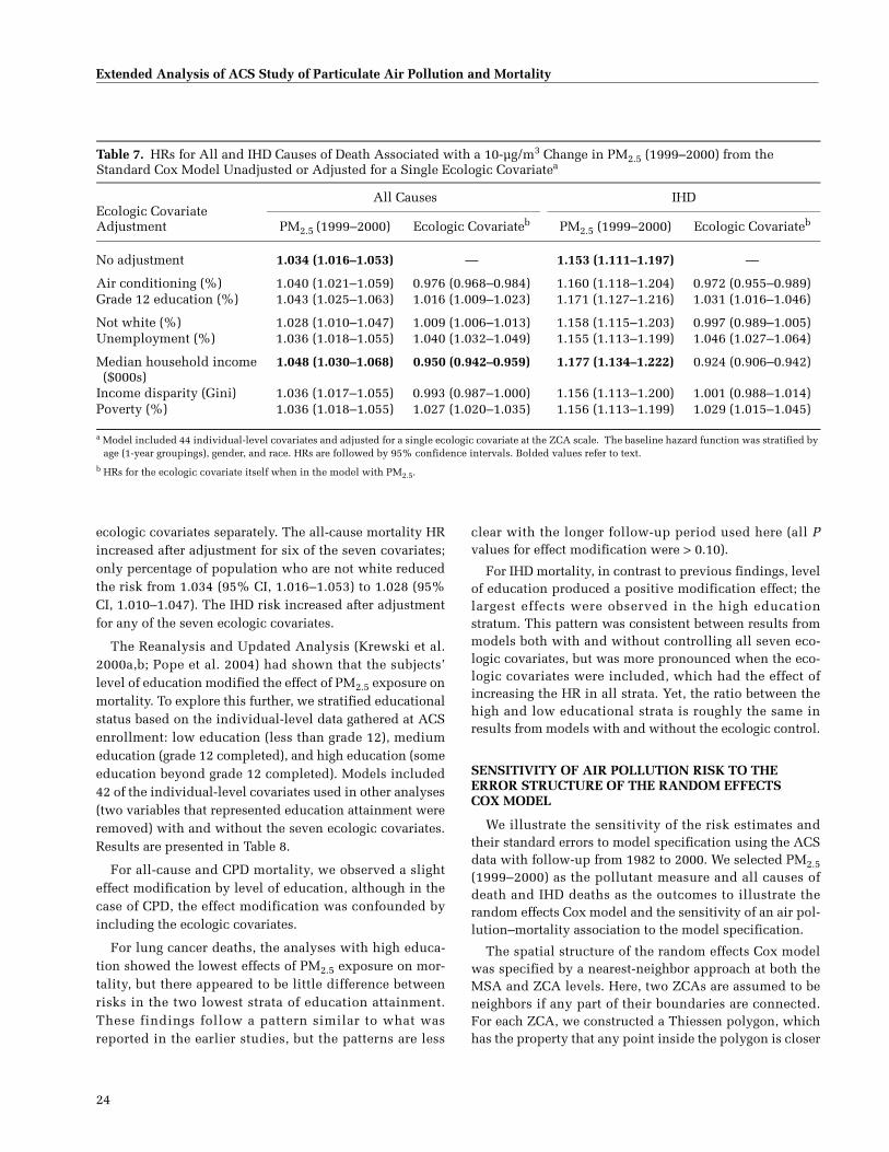
24
Extended Analysis of ACS Study of Particulate Air Pollution and Mortality
ecologic covariates separately. The all-cause mortality HRincreased after adjustment for six of the seven covariates;only percentage of population who are not white reducedthe risk from 1.034 (95% CI, 1.016–1.053) to 1.028 (95%CI, 1.010–1.047). The IHD risk increased after adjustmentfor any of the seven ecologic covariates.
The Reanalysis and Updated Analysis (Krewski et al.2000a,b; Pope et al. 2004) had shown that the subjects’level of education modified the effect of PM2.5 exposure onmortality. To explore this further, we stratified educationalstatus based on the individual-level data gathered at ACSenrollment: low education (less than grade 12), mediumeducation (grade 12 completed), and high education (someeducation beyond grade 12 completed). Models included42 of the individual-level covariates used in other analyses(two variables that represented education attainment wereremoved) with and without the seven ecologic covariates.Results are presented in Table 8.
For all-cause and CPD mortality, we observed a slighteffect modification by level of education, although in thecase of CPD, the effect modification was confounded byincluding the ecologic covariates.
For lung cancer deaths, the analyses with high educa-tion showed the lowest effects of PM2.5 exposure on mor-tality, but there appeared to be little difference betweenrisks in the two lowest strata of education attainment.These findings follow a pattern similar to what wasreported in the earlier studies, but the patterns are less
clear with the longer follow-up period used here (all Pvalues for effect modification were > 0.10).
For IHD mortality, in contrast to previous findings, levelof education produced a positive modification effect; thelargest effects were observed in the high educationstratum. This pattern was consistent between results frommodels both with and without controlling all seven eco-logic covariates, but was more pronounced when the eco-logic covariates were included, which had the effect ofincreasing the HR in all strata. Yet, the ratio between thehigh and low educational strata is roughly the same inresults from models with and without the ecologic control.
SENSITIVITY OF AIR POLLUTION RISK TO THE ERROR STRUCTURE OF THE RANDOM EFFECTS COX MODEL
We illustrate the sensitivity of the risk estimates andtheir standard errors to model specification using the ACSdata with follow-up from 1982 to 2000. We selected PM2.5(1999–2000) as the pollutant measure and all causes ofdeath and IHD deaths as the outcomes to illustrate therandom effects Cox model and the sensitivity of an air pol-lution–mortality association to the model specification.
The spatial structure of the random effects Cox modelwas specified by a nearest-neighbor approach at both theMSA and ZCA levels. Here, two ZCAs are assumed to beneighbors if any part of their boundaries are connected.For each ZCA, we constructed a Thiessen polygon, whichhas the property that any point inside the polygon is closer
Table 7. HRs for All and IHD Causes of Death Associated with a 10-µg/m3 Change in PM2.5 (1999–2000) from the Standard Cox Model Unadjusted or Adjusted for a Single Ecologic Covariatea
Ecologic Covariate Adjustment
All Causes IHD
PM2.5 (1999–2000) Ecologic Covariateb PM2.5 (1999–2000) Ecologic Covariateb
No adjustment 1.034 (1.016–1.053) — 1.153 (1.111–1.197) —
Air conditioning (%) 1.040 (1.021–1.059) 0.976 (0.968–0.984) 1.160 (1.118–1.204) 0.972 (0.955–0.989)Grade 12 education (%) 1.043 (1.025–1.063) 1.016 (1.009–1.023) 1.171 (1.127–1.216) 1.031 (1.016–1.046)
Not white (%) 1.028 (1.010–1.047) 1.009 (1.006–1.013) 1.158 (1.115–1.203) 0.997 (0.989–1.005)Unemployment (%) 1.036 (1.018–1.055) 1.040 (1.032–1.049) 1.155 (1.113–1.199) 1.046 (1.027–1.064)
Median household income ($000s)
1.048 (1.030–1.068) 0.950 (0.942–0.959) 1.177 (1.134–1.222) 0.924 (0.906–0.942)
Income disparity (Gini) 1.036 (1.017–1.055) 0.993 (0.987–1.000) 1.156 (1.113–1.200) 1.001 (0.988–1.014)Poverty (%) 1.036 (1.018–1.055) 1.027 (1.020–1.035) 1.156 (1.113–1.199) 1.029 (1.015–1.045)
a Model included 44 individual-level covariates and adjusted for a single ecologic covariate at the ZCA scale. The baseline hazard function was stratified by age (1-year groupings), gender, and race. HRs are followed by 95% confidence intervals. Bolded values refer to text.
b HRs for the ecologic covariate itself when in the model with PM2.5.

D. Krewski et al.
25
to the geographic center (centroid) of the ZCA than to thecentroid of any other ZCA. ZCA polygons were joined tocreate each MSA polygon; following this pattern, the 48contiguous United States were covered by polygons. Therandom effects associated with two MSAs (or ZCAs) areassumed to have a common correlation if they are neigh-bors and to be uncorrelated if they are not neighbors. TwoZCAs in different MSAs are assumed to be uncorrelated.
The HRs for a 10-µg/m3 change in PM2.5 (1999–2000) aregiven in Table 9 under selected error specifications for therandom effects Cox model with: (a) no adjustment for theseven ecologic covariates, (b) adjustment for the ecologiccovariates defined at only the ZCA level, and (c) adjust-ment for the covariates defined at both the MSA & DIFFlevels. All and IHD causes of death were examined.
Inclusion of clustering at both the MSA & DIFF levelsand at the ZCA level increased the estimate of the PM2.5(1999–2000) HR, with or without adjustment for the eco-logic covariates. This is likely due to the manner in whichthe random effects Cox model weights the importance ofthe observations. The standard Cox model gives equalweight to all subjects’ information whereas the randomeffects Cox model used here weights the information dif-ferently for each cluster. The variation in weight amongclusters is positively associated with the cluster variance.Thus the larger MSAs are given less weight in the randomeffects model than in the standard Cox model in whichresponses are assumed to be statistically independent. Anincrease in the HR using the random effects model impliesthat the larger MSAs did not clearly follow our model spec-ification, particularly the assumptions about there being a
log-linear relationship between mortality and the associ-ated exposure to PM2.5 (1999–2000). Thus they are givenless weight even though their sample size may be larger.
The inclusion of additional variance due to clustering ofsurvival experience at the MSA level also inflates theuncertainty in the PM2.5 (1999–2000) HR estimate, as evi-denced by wider confidence intervals (CIs) compared withthe case in which the MSA and ZCA variances are set to 0(equivalent to the standard Cox model assumption). Therewas more unexplained variation in survival between ZCAsthan between MSAs for all causes of death, but this patternis not replicated for IHD deaths.
Inclusion of the seven ecologic covariates defined at theZCA level reduced both the MSA and ZCA random effectsvariances. However, a further reduction was observedwhen these covariates were defined by their MSA & DIFFlevels together.
The inclusion of spatial autocorrelation at both the MSAand ZCA levels lowered the PM2.5 (1999–2000) HR and wid-ened the CIs, which suggests that there may be some evi-dence of spatial clustering of residual mortality coincidingwith the spatial pattern of PM2.5 (1999–2000). However, ourestimate of spatial autocorrelation at the MSA level (0.36)was at the boundary of allowable values. This implies thatthe model is ill-specified, likely due to the very largenumber of nearest neighbors for each MSA, particularly inthe Eastern U.S. Although we need to interpret these resultswith caution, we can view them as a situation with the max-imum spatial autocorrelation permissible, and thus weincluded them in our sensitivity analysis as an extreme case.
Table 8. Modification of HRs by Education at Individual Level for a 10-µg/m3 Change in PM2.5 (1999–2000) from the Standard Cox Model by Cause of Deatha
Level of Education / Participants (n)
Ecologic Covariates in Model All Causes CPD IHD Lung Cancer All Other Causes
< Grade 12 education(59,168)
No 1.064 (1.004–1.126) 1.127 (1.044–1.216) 1.111 (0.979–1.260) 1.187 (1.020–1.381) 0.955 (0.883–1.034)Yes 1.082 (1.024–1.144) 1.157 (1.077–1.245) 1.173 (1.022–1.347) 1.217 (1.025–1.446) 0.960 (0.886–1.040)
Grade 12 education (152,024)
No 1.060 (1.013–1.110) 1.086 (1.016–1.160) 1.195 (1.072–1.333) 1.192 (1.057–1.344) 0.999 (0.942–1.061)Yes 1.072 (1.020–1.127) 1.112 (1.040–1.189) 1.248 (1.109–1.404) 1.236 (1.081–1.413) 0.995 (0.931–1.062)
> Grade 12 education (274,941)
No 1.041 (1.001–1.083) 1.083 (1.023–1.146) 1.225 (1.121–1.339) 1.024 (0.912–1.150) 1.005 (0.956–1.058)Yes 1.055 (1.018–1.094) 1.115 (1.060–1.173) 1.331 (1.215–1.458) 1.043 (0.934–1.164) 1.006 (0.956–1.060)
a Model included 42 individual-level covariates (the two covariates for education attainment were omitted for this analysis) and with or without adjustment for the seven ecologic covariates at the MSA & DIFF levels together. The baseline hazard function was stratified by age (1-year groupings), gender, and race. HRs are followed by 95% confidence intervals. Bolded values refer to text. All P values > 0.10 for effect modification.

26
Extended Analysis of ACS Study of Particulate Air Pollution and Mortality
We also considered the sensitivity of our results to thespatial definition of clusters. Here, we used “state” and“MSAs within state” to define the cluster levels. There arefar fewer nearest neighbors for the state specification thanfor the MSA specification. We postulate that state is a nat-ural cluster definition because many health care programsand resources that influence health, and thus longevity, areadministered at the state level.
PM2.5 data for 1999–2000 were available for 44 states and116 MSAs. We included the 44 individual-level covariatesin random effects Cox models with adjustment for theseven ecologic covariates defined at the MSA & DIFFlevels together. Including both state and MSA-within-stateclusters increased the PM2.5 (1999–2000) HRs comparedwith results from the standard Cox model (Table 10, toprow under each cause of death) and also increased the
uncertainty in the estimates, as evidenced by the muchwider CIs. Including spatial autocorrelation at both clusterlevels reduced the HRs compared with a model thatincluded both state and MSA random effects but no spatialautocorrelation. Similar patterns were observed with andwithout adjustment for the ecologic covariates and for bothall causes of death and IHD deaths (results not shown).
ALTERNATIVE FORMULATION OF THE CONCENTRATION–RESPONSE FUNCTION
We investigated the form of the concentration–responsefunction between PM2.5 (1999–2000) and selected causesof death. Our alternative formulation of the function is thenatural logarithm of concentration. We selected this fortwo reasons. First, the logarithm of concentration yields a
Table 9. Sensitivity Analysis of the Deterministic and Stochastic Parameters of the Random Effects Cox Model for All and IHD Causes of Deatha
Ecologic Covariate Adjustment
HR for a 10-µg/m3 Change in PM2.5 (1999–2000)
MSA Variance(�10�3)
MSAAutocorrelation
ZCA Variance(�10�3)
ZCAAutocorrelation
All CausesStandard Cox modelNone 1.034 (1.016–1.053) 0 0 0 0ZCA 1.054 (1.035–1.075) 0 0 0 0MSA & DIFF 1.056 (1.035–1.078) 0 0 0 0
No autocorrelation at MSA or ZCA levelNone 1.057 (1.014–1.101) 1.62 0 4.35 0ZCA 1.080 (1.047–1.114) 1.21 0 3.06 0MSA & DIFF 1.075 (1.041–1.110) 0.95 0 3.01 0
Autocorrelation at MSA and ZCA levelsNone 1.048 (0.989–1.110) 1.66 0.36 5.65 0.29ZCA 1.074 (1.036–1.112) 1.25 0.36 3.61 0.23MSA & DIFF 1.071 (1.032–1.111) 1.06 0.36 3.45 0.22
IHDStandard Cox modelNone 1.153 (1.111–1.197) 0 0 0 0ZCA 1.210 (1.163–1.258) 0 0 0 0MSA & DIFF 1.240 (1.189–1.293) 0 0 0 0
No autocorrelation at MSA or ZCA levelNone 1.181 (1.092–1.278) 10.51 0 10.36 0ZCA 1.243 (1.147–1.346) 10.24 0 8.40 0MSA & DIFF 1.287 (1.179–1.404) 9.47 0 8.05 0
Autocorrelation at MSA and ZCA levelsNone 1.168 (1.065–1.280) 10.49 0.36 15.61 0.30ZCA 1.229 (1.120–1.347) 10.15 0.36 10.64 0.28MSA & DIFF 1.276 (1.156–1.409) 9.79 0.36 10.06 0.27
a Model included 44 individual-level covariates. The baseline hazard function was stratified by age (1-year groupings), gender, and race. A 0 indicates the parameter was not included in the model. HRs are followed by 95% confidence intervals.

D. Krewski et al.
27
flexible mathematical form to relate exposure to survivalwithin the proportional-hazards family of models. Herewe have
where the unknown parameter γ is a scalar. If � < 1, therelationship between PM2.5 and mortality concaves down-ward, which yields larger HRs at lower concentrations;and if � > 1, the association concaves upward, whichyields smaller HRs at lower concentrations. This formula-tion predicts HRs that are a function of concentration andthus a single risk value will not represent the associationbetween exposure and response throughout the concentra-tion range. The second reason is that the Updated Analysis(Pope et al. 2002) suggested that the logarithm of PM maybe a slightly better predictor of risk than the linear form.
The HRs associated with a 10-µg/m3 change in PM2.5
(1999–2000) concentrations based on linear and log-linearfunctions of PM are given in Table 11 for selected causesof death with and without adjustment for the seven eco-logic covariates defined at both the MSA & DIFF levelstogether. Two separate spans of a 10-µg/m3 change inPM2.5 are examined for the logarithmic formulation: from5 to 15 µg/m3 and from 10 to 20 µg/m3 since the HR basedon the logarithmic function varies with concentration. Aconcentration of 5 µg/m3 represents the minimum of thedistribution of PM2.5 (1999–2000) and a concentration of20 µg/m3 represents the 95th percentile of the concentra-tion distribution.
Our random effects Cox model was used to estimate theHRs with only one level of clustering at the MSA scale. ForPM2.5, the logarithmic function was a slightly better pre-dictor of the variation in survival among MSAs than thelinear function because the MSA random effect variance issomewhat smaller (than that for the linear function) foreach cause-of-death category except all other causes. As
� � � e r e e
t t U X( ) ( ) exp{log( ) }( ).
= +0 2 5PM
� � �e r e et t U X( ) ( ) exp( ) ( )( )
.= ∗0 2 5
PM
Table 10. Sensitivity Analysis of the Deterministic and Stochastic Parameters of the Random Effects Cox Model Due to Geographic Cluster Definition for All and IHD Causes of Deatha
Without or With Spatial Autocorrelation
HR for a 10-µg/m3 Change in PM2.5
(1999–2000)State Variance
(�10�3)State
AutocorrelationMSA Variance
(�10�3)MSA
Autocorrelation
All CausesStandard Cox model 1.056 (1.035–1.078) 0 0 0 0
Clustering by state onlyWithout 1.055 (1.019–1.092) 1.61 0 0 0With 1.045 (1.009–1.083) 1.90 0.23 0 0
Clustering by state and MSAWithout 1.072 (1.031–1.116) 1.22 0 0.32 0With 1.066 (1.021–1.112) 1.26 0.20 0.43 0.29
IHDStandard Cox model 1.240 (1.189–1.293) 0 0 0 0
Clustering by state onlyWithout 1.284 (1.189–1.387) 13.14 0 0 0With 1.232 (1.141–1.330) 14.04 0.39b 0 0
Clustering by state and MSAWithout 1.320 (1.192–1.460) 9.74 0 3.05 0With 1.241 (1.112–1.382) 8.83 0.39b 4.07 0.15
a Analysis based on 44 states and 116 MSAs. The model included 44 individual-level covariates and adjusted for seven ecologic covariates simultaneously. defined at the MSA and DIFF levels. The baseline hazard function was stratified by age (1-year groupings), gender, and race. A 0 indicates the parameter was not included in the model. HRs are followed by 95% confidence intervals.
b The estimation algorithm yielded a value of autocorrelation at the boundary of acceptable values, which indicates that the model was not properly specified and the results should be interpreted with caution.

28
Extended Analysis of ACS Study of Particulate Air Pollution and Mortality
expected, the HR based on the logarithm formulationyielded higher values for the difference between 5 and15 µg/m3 compared with the linear formulation; and lowervalues were observed for the difference between 10 and20 µg/m3 except for other causes of death in which the log-arithmic formulation yielded larger HRs compared withthe linear formulation.
The choice of functional relationship between PM expo-sure and mortality can make a considerable difference inthe predicted risk at lower concentrations. For example,the HR for lung cancer adjusted for the ecologic covariatesbased on the linear formulation is 1.142 (95% CI, 1.057–1.234), whereas the HR based on the logarithmic formula-tion is 1.236 (95% CI, 1.114–1.372), a 66% increase in risk.
DISCUSSION AND CONCLUSIONS
Our overall objective was to further analyze the associa-tion between particulate air pollution and all-cause andcause-specific mortality in large U.S. cities using alternative
spatial models and extended follow-up data from the ACSCPS-II cohort. Specifically, we examined whether social,economic, and demographic ecologic covariates confoundthe relationship between particulate air pollution andmortality, and we explored complex spatial patterns in theCPS-II data with an extended random effects Cox model.
Results of the Reanalysis Project showed that ecologiccovariates estimated on the MSA level were unlikely toexert a significant confounding influence on the associa-tion between particulate air pollution and mortality(Krewski et al. 2000a,b). Nevertheless, unresolved ques-tions remained about the scale and the construct validityof the variables used. Therefore, in the current study weexamined the influence of ecologic covariates at severalscales: the ZCA scale (data obtained from the 1980 U.S.Census), the MSA scale (by averaging information on allZCAs within an MSA), and by the value of the differenceobtained between the ZCA-specific value and the MSAvalue (DIFF).
Table 11. Comparison of HRs for Selected Causes of Death Associated with a 10-µg/m3 Change in PM2.5 (1999–2000) Concentrations Based on Inclusion of Linear PM2.5 or log(PM2.5) in the Random Effects Cox Model with Clustering at the MSA Levela
Ecologic Covariate Adjustment
Linear PM2.5 (1999–2000) Log (PM2.5 [1999–2000])
HR for10-µg/m3 Change
MSAVariance(�10�3)
HR forChange from 5 to 15 µg/m3
HR forChange from
10 to 20 µg/m3
MSAVariance(�10�3)
All CausesNone 1.060 (1.024–1.097) 1.86 1.095 (1.044–1.148) 1.059 (1.028–1.091) 1.81MSA & DIFF 1.078 (1.043–1.115) 1.07 1.128 (1.077–1.183) 1.079 (1.048–1.112) 1.00
CPDNone 1.094 (1.040–1.150) 3.96 1.145 (1.068–1.228) 1.089 (1.042–1.138) 3.87MSA & DIFF 1.128 (1.077–1.182) 1.86 1.208 (1.132–1.290) 1.127 (1.081–1.174) 1.66
IHDNone 1.196 (1.103–1.298) 12.13 1.315 (1.175–1.470) 1.188 (1.107–1.275) 11.73MSA & DIFF 1.287 (1.177–1.407) 10.56 1.484 (1.311–1.680) 1.283 (1.186–1.387) 9.80
Lung CancerNone 1.122 (1.040–1.210) 2.03 1.193 (1.071–1.330) 1.118 (1.044–1.197) 1.90MSA & DIFF 1.142 (1.057–1.234) 0.56 1.236 (1.114–1.372) 1.143 (1.071–1.221) 0.45
All Other CausesNone 1.008 (0.968–1.051) 1.95 1.023 (0.965–1.083) 1.014 (0.978–1.052) 1.97MSA & DIFF 1.010 (0.968–1.055) 1.37 1.026 (0.970–1.085) 1.016 (0.981–1.053) 1.39
a Model included 44 individual-level covariates with and without adjustment for seven ecologic covariates simultaneously. MSA & DIFF indicates both levels of data were included in the model together. The baseline hazard function was stratified by age (1-year groupings), gender, and race. HRs are followed by 95% confidence intervals. Bolded values refer to text.

D. Krewski et al.
29
Results from the CPS-II cohort with an additional elevenyears of follow-up in this Extended Analysis revealed pos-itive and significant associations between a 10-µg/m3
change in PM2.5 mass or a 5-µg/m3 in SO42� mass (with the
exception of SO42� [1990]) and all-cause, CPD, IHD, and
lung cancer deaths. Particles of larger size (PM15 and TSP)were associated with positive, although smaller, increasesin risk of all-cause, IHD, and CPD deaths. Mortality fromIHD compared with other causes of death was consistentlyassociated with the largest HR estimates. Indeed, otherrecent investigations have supported an associationbetween particles and adverse cardiovascular effects(Krewski et al. 2000a,b; Pope et al. 2004; Künzli et al.2005). Further investigations to examine the cardiovas-cular health effects of particulate air pollution are criticalto understanding the nature of the association.
Fewer significant associations were observed with thegaseous pollutants. SO2, which is likely to be an indicatorof other pollutants related to mortality, was significantlyassociated with higher mortality from all causes, CPD, andIHD, although the strength of the associations tended to beweaker than the associations observed with particles.Summertime O3 was related with all-cause and CPD mor-tality in this study; this relationship was statistically sig-nificant in the Reanalysis (relative risk = 1.08, 95% CI,1.01–1.16; Krewski et al. 2000a,b).
Due to differences in modeling methods and use ofmulti-level variables, HR estimates presented here are notdirectly comparable with the Updated Analysis usingalternate modeling strategies (Pope et al. 2002) or with theReanalysis (Krewski et al. 2000a,b), in which differentscales or levels of pollutant increases were used to calcu-late relative risks. This Expanded Analysis evaluated thelevel of risk associated with a 10-µg/m3 increase in PM2.5and a 5-µg/m3 increase in SO4
2�. The Reanalysis evaluateda 24.5-µg/m3 increase in PM2.5 and a 19.9-µg/m3 increasein SO4
2� (those values were equal to the difference inmean concentrations between the most- and least-pollutedcities from the Harvard Six Cities Study [Krewski et al.2000a]).
We wanted to directly compare the HRs between thethree follow-up periods that have been examined: 1982–1989 (the Reanalysis, Krewski et al. 2000a,b); 1982–1998(the Updated Analysis, Pope et al. 2002); and 1982–2000(the current Extended Analysis) (see also the sectionImplications of the Findings / Comparison of Data Sets andAnalytic Methods for the Three Follow-Up Time Periods).To do so, we estimated the HR for a 10-µg/m3 increase inthe average PM2.5 concentration for 1979–1983 in 58MSAs, and for 1999–2000 in 116 MSAs, and controlled forthe 44 individual-level covariates using the standard Cox
model (both with and without control for the ecologiccovariates) for mortality from all causes, CPD, IHD, lungcancer, and all other causes. Over the three follow-up timeperiods, deaths from all causes increased to 90,783 in the58 MSAs and 128,954 in the 116 MSAs; and deaths fromIHD increased to 20,651 in the 58 MSAs and 29,989 in the116 MSAs (see Table 32). For the PM2.5 (1979–1983) sam-pling period (58 MSAs), we observed a small decrease inthe HR estimate for deaths from all causes between the ini-tial follow-up period (1.048, 95% CI, 1.022–1.076) and thelater two periods (1.031, 95% CI, 1.015–1.047; and 1.028,95% CI, 1.014–1.043) (see Table 33). We found no temporalpattern in risk for IHD deaths (1.122, 95% CI, 1.066–1.181;1.130, 95% CI, 1.094–1.166; and 1.133, 95% CI, 1.100–1.167). Declining risk could be due to exposure misclassi-fication increasing over time. We assigned exposure basedon residence location in 1982; and the percentage of cohortmembers who have moved has to have increased overtime. Also, PM2.5 concentrations have clearly declinedover the follow-up period, so assigning a single exposuremeasure would not have fully captured this temporal pat-tern. Finally, as the cohort ages, air pollution effects maydecline due to the healthy survivor effect.
The ecologic covariates evaluated were associated withoverall and cause-specific mortality and correlated withspecific air pollutants, which is consistent with the defini-tion of a possibly confounding variable. Poverty andunemployment were positively associated and householdincome was negatively associated with all cause-of-deathcategories. Historically, indicators of community-levelsocioeconomic status such as these have been associatedwith overall and cause-specific mortality (Kaplan et al.1996; Boyd et al. 1999; Winkleby and Cubbin 2003). Theylikely reflect a complex interaction of environmental,social, and behavioral factors and of available health ser-vices that all influence health status and longevity. How-ever, income disparity (a related measure of economicstatus) was not associated with mortality in the ACS CPS-II cohort. This is surprising; we would have expectedincome disparity to be positively associated with mor-tality, as in some previous studies (Cooper et al. 2001; Ram2005; Singh and Siahpush 2006), although in the Reanal-ysis (Krewski et al. 2000a,b), income disparity was also notstrongly related with mortality. It may be that controllingthe 44 individual-level covariates (including such factorsas marital status, smoking, and diet) removed any poten-tial effect of income disparity on mortality in that study; orit may be that an inadequate variable was used.
All ecologic covariates were based on data from the1980 U.S. Census. Spatial patterns of mortality and ecolog-ically defined sociodemographic factors could change

30
Extended Analysis of ACS Study of Particulate Air Pollution and Mortality
independently of each other over follow-up time and thuslead to misclassification of their values and relationships.Discussion of the impact of population mobility in theACS cohort is presented elsewhere (Jerrett et al. 2007).Both the positive and negative influences of different eco-logic covariates on mortality require careful interpretationas to their potential confounding effects on the air pollu-tion–mortality association.
Spatial patterns of ecologically defined sociodemo-graphic factors and air pollution for the CPS-II cohort arecomplex. Ecologic covariates were both positively andnegatively correlated with concentrations of certain spe-cific air pollutants (see Table 4). Having less than a grade12 education was most frequently strongly correlated withair pollutant indices — negatively correlated with concen-trations of PM2.5 and SO4
2�, but positively correlated withparticles of larger size. Conversely, percentage of the pop-ulation that is not white and median household incomewas positively correlated with PM2.5 mass.
Correlations between ecologic covariates varied accord-ing to the unit of aggregation (ZCA or MSA), which indi-cates that spatial patterns in the data differ according toscale. Interestingly, the largest correlations were not neces-sarily found in the smallest unit of observation (ZCA) asmight be expected; this could indicate that complex spa-tial patterns of sociodemographic factors are also involved.Strong correlations were observed between some of theecologic covariates; therefore, caution is required in inter-preting models that include all of the ecologic covariatessimultaneously due to the possible resulting statisticalinstability.
Since variation in survival between subjects can beexplained, in part, by ecologic covariates that vary bothbetween and within MSAs, we conducted analyses thatadjusted for the ecologic covariates at both the MSA & DIFFlevels together. We hoped to account for sociodemographicrisks more completely and thus yield less biased risk esti-mates of exposure to air pollution. In nearly all models thatadjusted for the seven ecologic covariates simultaneously,the HR tended to increase in comparison to models with noadjustment, although many of the differences were small.The largest increases were observed for mortality from IHDassociated with PM2.5 (1999–2000) and SO4
2� (1990); themagnitude of the inflation of HR was 7.5% and 12.8%,respectively; this model included ecologic covariates atboth the MSA & DIFF levels simultaneously.
When we evaluated the independent effect of each eco-logic covariate at the ZCA scale on the HR for the associationbetween PM2.5 and mortality from all causes and from IHD,we found that each covariate independently increased thestrength of the association (except for percentage who are
not white with all-cause mortality). We found the largestincreases when household income was the only ecologiccovariate included — from 1.034 (1.016–1.053) to 1.048(1.030–1.068) for all causes of death, and from 1.153(1.111–1.197) to 1.177 (1.134–1.222) for deaths from IHD(Table 7). Household income was positively associatedwith exposure to PM2.5 (1999–2000) and negatively associ-ated with all-cause mortality. (No individual-level infor-mation on income was available for CPS-II participants;therefore, we relied on the ecologic-level indicator ofincome status.)
Percentage of the population with a grade 12 educationexerted the next largest influence on HR estimates. Therandom effects Cox model was adjusted for educationattainment at the individual level. This analysis, therefore,suggests that neighborhood education attainment mea-sured at the ZCA level exerts additional influence on theair pollution–mortality association beyond that of indi-vidual-level education attainment.
ZCA-level median household income and grade 12 edu-cation, therefore, represent the most important sociodemo-graphic ecologic factors that may confound the PM2.5–mortality association, although their effects individuallyare slight.
One of the more remarkable findings in this set of anal-yses was that when ecologic covariates were included, theHRs increased. This finding likely represents a case of vari-ance suppression (Tabachnick and Fidell 2001), which isdocumented as one way in which confounding variablesmay increase the size of their effects on the primary riskvariable in the model. Ecologic confounders and the pollut-ants share some of the model variance, and their commonvariability also partially overlaps with the variability of themortality outcome. The part of the variance shared by theecologic and pollutant variables is the component of vari-ance with mortality that has a relatively less-defined asso-ciation with pollution. When the ecologic covariates areincluded in the model, the component of the varianceoverlap between pollution and mortality is removed, andthe remaining relationship becomes more pronounced.These results imply that simultaneous consideration ofecologic covariates and air pollution may be important inmodels of chronic health effects.
Results from the Reanalysis (Krewski et al. 2000a,b) sug-gested that SO2 may exert a more robust effect on mortalitythan SO4
2�. In the current Extended Analysis, includingecologic covariates at multiple scales exerted little influ-ence on HR estimates for the association between SO2 andall-cause and cause-specific mortality. An exception wasfor IHD mortality, in which including ecologic covariates

D. Krewski et al.
31
at the MSA & DIFF levels together increased the HR valueslightly (by 2.1%).
The ecologic covariates exerted their greatest effect onmortality from IHD, which was also the outcome moststrongly related with PM2.5 (1979–1983 and 1999–2000),SO4
2� (1980–1981 and 1990), and SO2 exposure, and wasthe only outcome significantly associated with NO2 expo-sure. IHD, a significant contributor to mortality in theUnited States, is associated with a multitude of behavioralrisk factors such as smoking, lack of exercise, obesity, anddiet, which are likely related to spatial patterns in sociode-mographics such as income, education level, and unem-ployment. Spatial patterns in health services available todiagnose and treat IHD are possibly another importantfactor not explicitly evaluated here. The HR of IHD mor-tality associated with air pollution exposure remained ele-vated even after adjustment for a variety of individual-level and ecologic covariates. The fact that IHD mortalitywas the outcome most influenced by the ecologic covari-ates suggests the importance of controlling for these influ-ences in future studies.
Another interesting finding was the fact that, in general,the geographic unit of analysis (ZCA or MSA) of ecologiccovariates tended to not make an appreciable difference intheir influence on HR estimates. In many cases, though,HR estimates tended to be highest from models with theecologic covariate considered at the MSA & DIFF levelssimultaneously. The sociodemographic ecologic covariatesat simply the ZCA or MSA levels, compared with the MSA& DIFF levels, did not substantially alter results of the airpollution–mortality association found in the current study.
The association between air pollution and lung-cancermortality was found to vary somewhat by level of educa-tion attainment recorded at the inception of the cohort.The risk of lung-cancer mortality associated with each 10-µg/m3 change in PM2.5 (as measured in 1999–2000) wasapproximately 20% higher for participants who completedonly grade 12 education compared with no associationobserved among those who completed more than highschool. Including ecologic covariates increased the pointestimates and width of CIs slightly. Similar results werereported in the Reanalysis (Krewski et al. 2000a,b): relativerisks of 1.41 (95% CI, 0.87–2.29) and 1.39 (95% CI, 0.90–2.15) were reported for lung-cancer mortality associatedwith each 24.5-µg/m3 change in PM2.5 among those whocompleted less than high school and those who completedhigh school, respectively, whereas a relative risk of 0.66(95% CI, 0.46–0.95) was found among those who com-pleted more than high school. Indeed, this finding ofincreasing mortality from PM2.5 exposure associated withdeclining education attainment represented a key finding
of the Reanalysis. In the Updated Analysis, Pope andcoworkers (2002) also reported a similar trend. Althoughthe reasons for this finding are unknown, it was suggestedthat level of education attainment may likely indicate theeffects of complex and multifactorial socioeconomic pro-cesses on mortality or may reflect disproportionate pollu-tion exposures.
Although the direction of the trend for all-cause andCPD mortality in the current study was similar to that oflung-cancer mortality, a significantly elevated HR wasfound for these outcomes in each educational stratum andthe magnitude of the difference was small. This suggeststhat education attainment may exert less of a modifyingforce on these mortality categories. A surprising finding inthe current study was increasing IHD mortality associatedwith PM2.5 (1999–2000) and increasing education attain-ment (Table 8). HR estimates for IHD mortality alsoincreased up to 11% among those with more than highschool education with the inclusion of ecologic covariatesin the model. Large socioeconomic differences in coronarymortality have been observed in the United States, whereindividuals of lower socioeconomic status exhibit greatercoronary mortality compared with individuals of highersocioeconomic status (Kunst et al. 1999; Mackenbach et al.2001; Armstrong et al. 2003). The finding of a greater effectof PM2.5 exposure on IHD mortality among those withgreater education attainment in the current study may sug-gest that there are a number of individual- or community-level influences on mortality among those with lower edu-cation that are more powerful than that of PM2.5.
We also explored complex spatial patterns in the CPS-IIdata. The 2000 Reanalysis, using a random effects Coxmodel that could handle up to two levels of clustering,showed that spatial risk models attenuate the air pollutioneffect, both in terms of size and certainty. The presence ofspatial autocorrelation has important implications withrespect to bias and precision of model-based estimates ofrisk. In this project we extended the random effects Coxmodel used in the Reanalysis to be capable of handlingmore than two levels of clustering in order to evaluate howrobust the results from the Reanalysis would be to moresophisticated spatial models.
The spatial random effects Cox model captures addi-tional variation beyond that explained by the standard Coxmodel. We included random effects at both the MSA andZCA levels in order to capture variation in survival due tounexplained variation between MSAs and between ZCAswithin MSAs. We note that including these random effectstends to increase the estimated HR of death associated withair pollution exposure and to inflate uncertainty in theseestimates, as evidenced by wider confidence intervals.

32
Extended Analysis of ACS Study of Particulate Air Pollution and Mortality
We further note that including the ecologic covariatesdecreases the variance of the random effects at both theMSA and ZCA level; the largest decrease in residual varia-tion is based on models with the MSA & DIFF specification,which suggests that partitioning the ecologic covariates intobetween-MSA and within-MSA values more completelycaptures these sources of variation.
INTRA-URBAN ANALYSIS FOR THE NEW YORK CITY REGION
A LAND-USE REGRESSION MODEL FOR PREDICTING PM2.5 CONCENTRATIONS
Background
Exposure to PM2.5 has been linked to a wide array ofhealth outcomes such as aggravation of existing heart andlung disease and premature death (Pope et al. 2002). Suchhealth studies, though, often rely on pollutant exposureestimates that are based on a city’s central monitors; thatsame level of exposure is then assigned to the entire popu-lation in a metropolitan area and exposure estimates arecompared between cities. Recent studies of PM2.5 haveshown, however, that intra-urban exposure gradients canalso be associated with atherosclerosis (Künzli et al. 2005)and with high risk of premature death (Jerrett et al. 2005a).These studies have used geostatistical interpolation modelsthat capture regional patterns of pollution well, but oftenfail to account for the near-source impact from local trafficand industry. Given the high risks of health effects reportedin these studies and others conducted in Europe (Hoek etal. 2002; Nafstad et al. 2003), we need to refine the esti-mates of pollutant exposures and reduce uncertainties thatcould be associated with measurement error.
Several recent studies have demonstrated the potentialof LUR to supply accurate, small-area estimates of air pol-lutant concentrations without the financial expense of dis-persion or exposure modeling (Brauer et al. 2003; Briggs etal. 2000a). The goal of LUR is to explain, to the extent pos-sible, the variation in existing air quality data for a givenpollutant using data on nearby traffic, land use, emissionsfrom local sources, and population variables. In most cases,multiple linear regression is used to develop and validate amodel using data from existing monitors and land-use datathat can then be applied to unmonitored locations pro-vided the appropriate geographic data are available.
Ross and associates (2006) developed LUR models usingtraffic data, distance to the coast, and road length measure-ments to predict NO2 levels in San Diego, California, that
explained nearly 80%of the variation in measured expo-sure levels. When the predicted levels were comparedwith measured levels at validation locations — locationsthat were not included in developing the model — theywere accurate to within, on average, 2.1 ppb. LUR modelsto predict NO2 levels using traffic and other variables inMontréal and several European cities also produced accu-rate predictions (Jerrett et al. 2005b).
In contrast to a more localized pollutant such as NO2,however, PM mass has a significant regional componentthat includes smaller contributions from local sources(Bari et al. 2003). This complicates estimating intra-urbanexposure with LUR. Models of PM2.5 in three Europeancities produced mixed results. One of the only studies toattempt prediction of fine particle concentrations with theLUR methods to date was undertaken in Europe as part ofthe TRAPCA (Brauer et al. 2003). Researchers measuredPM2.5 for representative temporal periods over one year inthe Netherlands; Munich, Germany; and StockholmCounty, Sweden. They found significant differences in theability of the model to predict monitoring data from regionto region: values from LUR models could predict from73% of the variation of monitored values (the Netherlands)down to 56% and 50% (Munich and Stockholm, respec-tively). The limited variability of the monitoring sites inStockholm County was suggested as an explanation for thedifference in the Stockholm data (Brauer et al. 2003).When combined with health data, an LUR model was ableto predict some childhood respiratory outcomes (Brauer etal. 2002). More recently, in Germany, Hochadel andcoworkers (2006) found that LUR predicted PM2.5 absor-bance (R2 = 65%–82%), but failed to predict PM2.5 massvery well (R2 = 9%–17%).
North American cities have vastly different transporta-tion and land-use patterns than those in Europe, and theapplicability of LUR to predict PM2.5 is unknown (Gilbertet al. 2005). To our knowledge this study was the firstattempt to apply LUR to analyze PM2.5 in North America.
Materials and Methods
LUR uses concentrations of ambient pollutants at moni-toring locations as the dependent variable. Surroundingland-use, transportation, emissions from local sources,and population data were obtained using GIS andincluded in a regression equation as predictor variables. Inthis study we assembled a database of information on landuse and transportation around the PM2.5 monitors in theNew York City region.
We constructed three models: one covering a 9-countyurban area using 3-year averages; another covering all28 counties using 3-year averages; and a third covering the

D. Krewski et al.
33
28 counties using data for only the winter months of 2000.After describing the data we collected, we present our sta-tistical modeling strategy.
Dependent Variable: Ambient PM2.5 Data For the 28-county models, counties were chosen to match thoseincluded in the Best Practice Model (BPM; a tool for fore-casting regional travel demand) used by the New York Met-ropolitan Transportation Council (NYMTC), the regionalcouncil of governments established to help make transpor-tation-related decisions in the region. Of those, 9 countieswere selected to represent the more urbanized area of NewYork City’s five boroughs and adjacent New Jersey andConnecticut counties.
In general, the 28 counties ranged from very urban torelatively rural; 12 counties had fewer than 500,000 people(with a minimum population of 96,000 in Putnam County)and 6 counties had more than 1,000,000 people (maximumpopulation of 2,470,000 in Kings County). Most countieshad heavily urban populations (based on population persquare mile) — the populations were greater than 90%urban in 22 counties and greater than 99% in 12 of those.The 6 least-urban counties (Hunterdon, Warren, Sussex,Orange, Dutchess, and Putnam), all of which are more than50 km west or north of downtown Manhattan, range from40%–76% urban. For comparison, the average county pop-ulation for the three states is 340,000 and the averageurban percentage is 64%.
We calculated 3-year averages (from data in 1999–2001)of PM2.5 for monitors in the 28-county region around NewYork City (Figure 1) using data from the U.S. EPA AirQuality Subsystem (AQS; a repository for ambient airquality data made available for analysis). For each monitorthat had at least eight observations in a quarter (i.e., at leasthalf of the scheduled monitoring days), we first computedquarterly means. When we could calculate a complete setof four quarterly means for three years running, we com-puted 3-year averages from the 12 quarterly means. (We lostonly about 5% of the monitors due to incomplete data.)
We were also interested in assessing seasonal variationsin exposure, especially for SO4
2�. New York City experi-ences long-range transport of secondary aerosols with ahigh proportion of SO4
2� in the warmer months. BecauseSO4
2� is also formed regionally, the exposure gradientwithin cities is more spatially homogenous during thewarmer months when secondary aerosols are transported.By contrast, in the winter months, SO4
2� concentrations arestrongly influenced by local emissions from automobile andtruck traffic, shipping, heating, and industry. The exposuregradient within the city is therefore generally steeperduring the winter months when the dominant regional
exposure is absent. The steeper gradients increase the sta-tistical power of our health effects models to detect associ-ations between air pollution and mortality.
Thus, for winter of 2000 in 28 counties, we computedpollutant averages using data from January, February, andMarch. We limited the winter-2000 analysis to those sitesthat could provide both 3-year and winter-2000 averages.Data from 62 monitors in the 28-county region wereincluded in the 3-year analysis of the 28-county area (1999–2001), data from 36 in the 3-year analysis of the 9-countyarea (1999–2001), and data from 45 for the 28-county area inwinter (2000).
At nine monitoring locations, two types of monitorswere used concurrently: the Federal Reference Method(FRM) and the tapered-element oscillating microbalance(TEOM) continuous monitoring method. When both TEOMand FRM data were collected at the same site, we used theFRM data.
For most monitors, the AQS included latitudes and lon-gitudes for the monitors, but some were inaccurate. Wetherefore used locations provided directly by the appro-priate state agencies (the Department of EnvironmentalConservation in New York and the Departments of Envi-ronmental Protection in New Jersey and Connecticut). Inmost instances, the locations were identified by the agen-cies with either a global positioning system (GPS) or ortho-photos in a GIS. For a limited number of older sites, themore accurate methods had not been used by the agencies,so we manually verified their locations in a GIS using acombination of road layers, orthophotos, New York StateDepartment of Transportation Raster Quadrangles, andUSGS Digital Raster Graphics.
Independent Variables: Traffic, Land-Use, Population, and Local Emissions Data For each air monitoring loca-tion in the AQS for which we had adequate data on PM2.5,using our GIS software we generated circular buffersaround the monitor location with different radii (50 m, 100m, 300 m, 500 m, and 1000 m). All of the mapped data inour GIS layers (as described below) were then linked withthe circular buffers, and the traffic and land-use data for allbuffers around each air monitoring location were calcu-lated. Calculations were performed with a vector datastructure using ArcGIS 9.1 (ESRI 2004).
Traffic and Road Data The NYMTC provided trafficestimates for 2002 for New York City and surroundingcounties that covered approximately 40,000 road links in28 counties using the BPM, a tool used for forecastingregional travel demand in the metropolitan area. TheBPM makes use of traffic data from more than a dozen

34
Extended Analysis of ACS Study of Particulate Air Pollution and Mortality
municipal and other sources. The road network used inthe BPM was developed to include all minor arterial roadsor larger from five separate network databases. The fivehad been conflated to match the LION street centerline filefor New York’s five boroughs (from the City of New YorkDepartment of City Planning 2009) and the USCB Topolog-ically Integrated Geographic Encoding and ReferencingDatabase. A complete description of the BPM model anddevelopment of mapped roadways can be found in ParsonsBrinckerhoff Quade & Douglas, Inc. (2005). The traffic esti-mates, divided by vehicle type (heavy- and light-dutytrucks, buses, vans, cars), are available for the four timeperiods of morning, midday, afternoon, and night. We usedestimates for afternoon rush-hour traffic flow because acomplete set of estimates (for all 40,000 links) for theother time periods was not yet available. We calculatedtotals for truck traffic and total traffic for each buffer zonearound each monitor. Traffic data were scaled to 1000s ofvehicle-kilometers per hour. We also used this data source
to calculate road density (total length of roadway in kilo-meters) in each buffer area.
Land-Use Data Layers of land-use data were assembledfrom several sources: extremely detailed (1 inch = ~250feet) tax-lot data from the New York City Department ofCity Planning for all tax lots in the five boroughs (2003);medium-scaled (1 inch = ~40,000 feet) land-use data forNew Jersey from the New Jersey Department of Environ-mental Conservation (1995/1997); and coarse scale (1 inch= ~100,000 feet) land-use data from the USGS NationalLand Cover Data 1997 (based on Landsat satellite imagesfrom 1992 and confirmed using aerial photos). For eachland-use layer we calculated the total area of an individualland-use category (e.g., industrial, forest, residence) ineach buffer. Although the tax-lot and New Jersey land-usedata layers were more detailed, only the data from theUSGS covered the entire area of interest.
Figure 1. Locations of PM2.5 monitors in the New York City region.

D. Krewski et al.
35
Similar uses within each land-use layer were grouped tocreate aggregate variables. The land-use categories withinthe three layers were not identical but comparable group-ings were tabulated. We generated industrial and residen-tial categories from all three land-use layers. In addition,for the New Jersey Department of Environmental Conser-vation data and the National Land Cover Data, we createdwater, vegetation, and barren land-use variables.
The “Industrial” category, discussed throughout most ofthis section, comprises the “Industrial / Commercial /Transportation” category from USGS data and the NewJersey land-use data. We created a comparable groupingusing the New York City tax-lot data by combining the cate-gories denoted “Industrial and Manufacturing”, “Transpor-tation and Utility” and “Commercial and Office Buildings.”The New York City tax-lot data and the New Jersey land-usedata were used only for sensitivity analysis because theydid not cover the entire region. Land-use areas were con-verted to acres (1 acre = 4047 m2).
Population Data Census data for the New York Citystudy area were acquired at the block-group level fromthe USCB 2000 Summary File 1 (for population andhousing data) and Summary File 3 (for income data). Allpopulation and housing data are in 1000s or percentages;income data were not scaled (U.S. Census Bureau 2000).These data were used as possible predictor variables inthe LUR model.
Local Emissions Data We calculated primary emissionsof PM2.5 (area, point, off-road mobile, and on-road mobile)for each county and assigned to each monitor the valueassociated with its county as a possible predictor variable.In addition, for each buffer area, we calculated the numberof point sources and the amount of PM2.5 emissions using
data for 1999 from the U.S. EPA National Emissions Inven-tory (1999).
Statistical Data Analysis We developed three separatemodels: two that included data from all 28 counties, one ofwhich used the 3-year-average PM2.5 data and one thatused the winter-2000 PM2.5 data; and a third that used 3-year-average PM2.5 but was geographically limited to thenine more urbanized counties.
We started with 62 monitors in the 28 counties. First,based on each monitor’s land-use code in the AQS, wedivided them into agricultural/forest, commercial, indus-trial/mobile, and residential categories. Next, to validateour predictions later, we randomly removed 20% of themonitors to use for validating the predictions that wouldbe generated. Samples (monitors) were removed from eachof the 28-county and 9-county models separately using thesame criteria. The remaining monitors were used todevelop the models.
The 28-county 3-year model included 49 monitors fordeveloping the model (plus 13 removed for validation; 62total), the 28-county winter-2000 model included 36 moni-tors for modeling (plus 9 removed for validation; 45 total),and the 3-year 9-county model included 29 monitors formodeling (plus 7 removed for validation; 36 total) (Table 12).
We then considered more than 25 separate variableswithin five different buffer distances around each monitorfor possible inclusion in the final three models. Theseincluded total traffic, total truck traffic, industrial landuse, residential land use, total county-wide emissions,point emissions, total number of point sources of PM2.5,total population, number of housing units, median incomeof population, and the percentage of the population whoare not white.
Table 12. Modeling and Validation Monitors by Land-Use Category
Land-Use Categorya
3-Year Models
Winter-2000 Average
28-CountyTotal
28-CountyValidation
9-CountyTotal
9-CountyValidation
28-CountyTotal
28-CountyValidation
Industrial / mobile 8 2 6 1 5 1Residential 32 6 19 4 24 5Commercial 18 4 11 2 12 2Agricultural / forest 4 1 0 0 4 1
Total 62 13 36 7 45 9
a Based on codes in the U.S. EPA’s AQS.
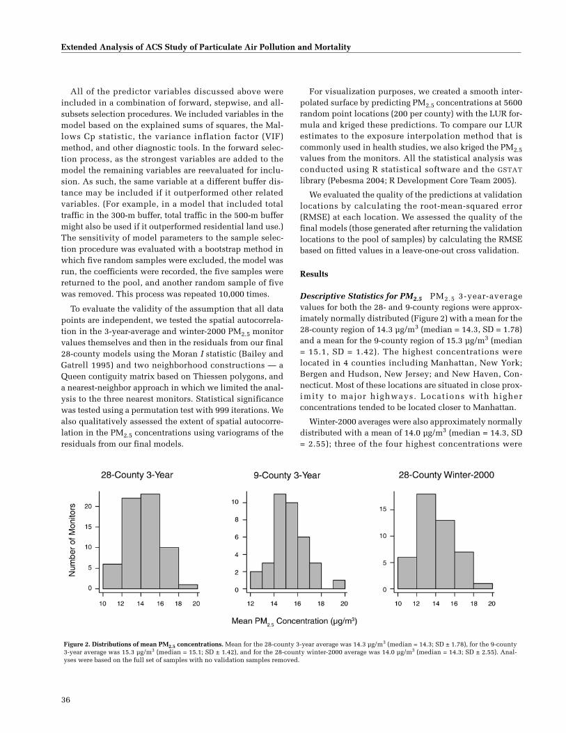
36
Extended Analysis of ACS Study of Particulate Air Pollution and Mortality
All of the predictor variables discussed above wereincluded in a combination of forward, stepwise, and all-subsets selection procedures. We included variables in themodel based on the explained sums of squares, the Mal-lows Cp statistic, the variance inflation factor (VIF)method, and other diagnostic tools. In the forward selec-tion process, as the strongest variables are added to themodel the remaining variables are reevaluated for inclu-sion. As such, the same variable at a different buffer dis-tance may be included if it outperformed other relatedvariables. (For example, in a model that included totaltraffic in the 300-m buffer, total traffic in the 500-m buffermight also be used if it outperformed residential land use.)The sensitivity of model parameters to the sample selec-tion procedure was evaluated with a bootstrap method inwhich five random samples were excluded, the model wasrun, the coefficients were recorded, the five samples werereturned to the pool, and another random sample of fivewas removed. This process was repeated 10,000 times.
To evaluate the validity of the assumption that all datapoints are independent, we tested the spatial autocorrela-tion in the 3-year-average and winter-2000 PM2.5 monitorvalues themselves and then in the residuals from our final28-county models using the Moran I statistic (Bailey andGatrell 1995) and two neighborhood constructions — aQueen contiguity matrix based on Thiessen polygons, anda nearest-neighbor approach in which we limited the anal-ysis to the three nearest monitors. Statistical significancewas tested using a permutation test with 999 iterations. Wealso qualitatively assessed the extent of spatial autocorre-lation in the PM2.5 concentrations using variograms of theresiduals from our final models.
For visualization purposes, we created a smooth inter-polated surface by predicting PM2.5 concentrations at 5600random point locations (200 per county) with the LUR for-mula and kriged these predictions. To compare our LURestimates to the exposure interpolation method that iscommonly used in health studies, we also kriged the PM2.5values from the monitors. All the statistical analysis wasconducted using R statistical software and the GSTAT
library (Pebesma 2004; R Development Core Team 2005).
We evaluated the quality of the predictions at validationlocations by calculating the root-mean-squared error(RMSE) at each location. We assessed the quality of thefinal models (those generated after returning the validationlocations to the pool of samples) by calculating the RMSEbased on fitted values in a leave-one-out cross validation.
Results
Descriptive Statistics for PM2.5 PM2.5 3-year-averagevalues for both the 28- and 9-county regions were approx-imately normally distributed (Figure 2) with a mean for the28-county region of 14.3 µg/m3 (median = 14.3, SD = 1.78)and a mean for the 9-county region of 15.3 µg/m3 (median= 15.1, SD = 1.42). The highest concentrations werelocated in 4 counties including Manhattan, New York;Bergen and Hudson, New Jersey; and New Haven, Con-necticut. Most of these locations are situated in close prox-imity to major highways. Locations with higherconcentrations tended to be located closer to Manhattan.
Winter-2000 averages were also approximately normallydistributed with a mean of 14.0 µg/m3 (median = 14.3, SD= 2.55); three of the four highest concentrations were
Figure 2. Distributions of mean PM2.5 concentrations. Mean for the 28-county 3-year average was 14.3 µg/m3 (median = 14.3; SD ± 1.78), for the 9-county3-year average was 15.3 µg/m3 (median = 15.1; SD ± 1.42), and for the 28-county winter-2000 average was 14.0 µg/m3 (median = 14.3; SD ± 2.55). Anal-yses were based on the full set of samples with no validation samples removed.

D. Krewski et al.
37
located in Manhattan and one in New Haven. These statis-tics are based on the full set of samples with no validationsamples removed.
LUR Model Building and Results
28-County and 9-County Models Based on 3-Year-AverageConcentrations For both regions, the total traffic variablewas the strongest predictor of PM2.5 concentrations (seeTable 13 for distributional statistics on final predictors).Total traffic in the 500-m buffer and total traffic in the 300-m buffer, in particular, led all other variables in explana-tory power. Urbanization-related variables, primarily inthe 500- and 1000-m buffers, were also strong predictors ofPM2.5 concentrations both with and without total traffic inthe 500-m buffer included in the model. These includedtotal population in both the 500- and 1000-m buffers andnumbers of both households and housing units in the1000-m buffer.
With total traffic in the 500-m buffer and total popula-tion in the 500-m and 1000-m buffers in the model, thenext strongest predictor was industrial land use in the 300-m buffer for both the 28-county and 9-county regions.
The final models for both of these regions thereforeincluded total traffic in the 500-meter buffer, total popula-tion in the 1000-meter buffer, and industrial land use inthe 300-meter buffer (Table 14).
The 28-county 3-year model predicted PM2.5 at valida-tion locations to within, on average, 0.93 µg/m3 (6.5%) ofactual concentrations with a RMSE of 1.10. The 9-countymodel predicted PM2.5 at validation locations to within,on average, 0.77 µg/m3 (5.0%) of actual concentrationswith a RMSE of 0.87. The predictions for validation sitesshowed some bias, particularly in the 28-county 3-yearmodel, which was likely to over-predict PM2.5 values,
though no bias was apparent in the models after includingthe validation samples (Figure 3).
Within the 28-county 3-year model, the predictionswere better for those validation sites located in the moreurbanized 9-county area. The nine validation sites locatedwithin the 9 counties had a RMSE of 0.90, whereas the foursites located in the other 19 counties had a RMSE of 1.45.This distinction, however, is due primarily to a single largeresidual in Waterbury, Connecticut, at a site with thesecond highest industrial land use among all the 62 loca-tions in the 28-county area and relatively high traffic.
When the validation samples were returned to the poolof modeling samples and the models were run again, theregression parameters remained similar; the parameter forthe industrial land-use variable changed most betweenruns. The average absolute value residuals based on thefitted values (for observations included in the modelingrather than the prediction of validation locations) from thefull models (no excluded samples) were 0.85 µg/m3 or6.0% of actual concentrations for the 28-county 3-yearmodel (with an RMSE based on a leave-one-out cross vali-dation of 1.15), and 0.69 µg/m3 or 4.5% of actual concen-trations for the 9-county 3-year model (RMSE of 1.00). Thefinal 28-county 3-year model explained 64% of the varia-tion in the PM2.5 measured values from the validationlocations, and the 9-county 3-year model explained 62%of the variation. Plots of the fitted and observed values arepictured in Figure 4.
Models included data from a mix of FRM and TEOMmonitors: for the 28-county 3-year model, 50 FRM and 12TEOM; for the winter-2000 model, 42 FRM and 3 TEOM;for the 9-county 3-year model, 25 FRM and 11 TEOM.Although plots of the nine sampling locations with bothFRM and TEOM monitors showed little or no bias (four
Table 13. Distribution Statistics for Final Predictor Variablesa
28-County 3 Years 9-County 3 Years 28-County Winter-2000
TotalTraffic (500 m)
TotalPopulation (1000 m)
Industrial Land Use (300 m)
TotalTraffic (500 m)
TotalPopulation (1000 m)
Industrial Land Use (300 m)
TotalTraffic (300 m)
TotalPopulation (1000 m)
Vegetation Land Use (1000 m)
Minimum 0.00 0.21 0.00 0.00 0.21 0.00 0.00 0.21 4.921st quartile 1.46 6.31 1.17 2.41 16.75 3.40 0.33 6.09 31.36Median 4.55 14.53 9.23 5.38 36.47 7.87 1.07 11.19 96.66
Mean 6.41 27.52 14.26 8.03 42.60 12.85 2.21 22.97 125.903rd quartile 9.80 42.28 20.34 13.48 55.01 16.59 3.83 27.22 122.10Maximum 24.06 119.40 52.70 24.06 119.40 45.77 8.35 119.40 697.10
a Traffic units: 1000s of vehicle-km/hour; total population units: 1000s of people; land-use units: acres.
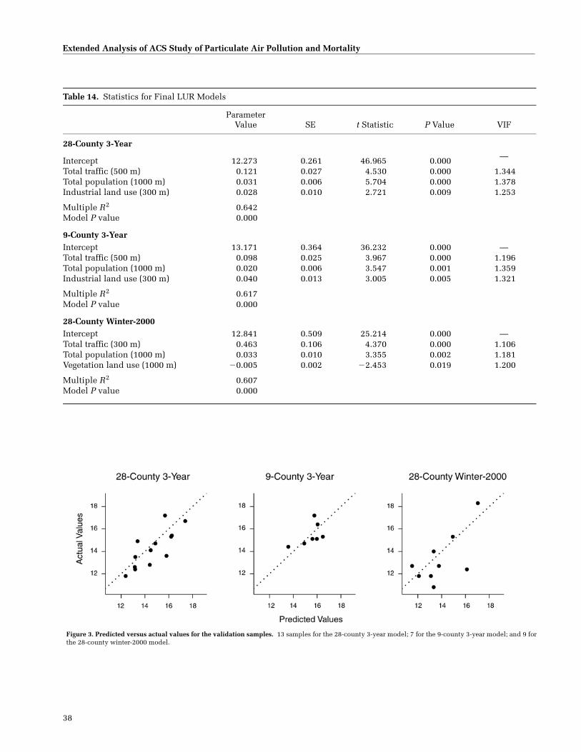
38
Extended Analysis of ACS Study of Particulate Air Pollution and Mortality
Table 14. Statistics for Final LUR Models
ParameterValue SE t Statistic P Value VIF
28-County 3-Year
Intercept 12.273 0.261 46.965 0.000 —
Total traffic (500 m) 0.121 0.027 4.530 0.000 1.344Total population (1000 m) 0.031 0.006 5.704 0.000 1.378Industrial land use (300 m) 0.028 0.010 2.721 0.009 1.253
Multiple R2 0.642Model P value 0.000
9-County 3-YearIntercept 13.171 0.364 36.232 0.000 —Total traffic (500 m) 0.098 0.025 3.967 0.000 1.196Total population (1000 m) 0.020 0.006 3.547 0.001 1.359Industrial land use (300 m) 0.040 0.013 3.005 0.005 1.321
Multiple R2 0.617Model P value 0.000
28-County Winter-2000Intercept 12.841 0.509 25.214 0.000 —Total traffic (300 m) 0.463 0.106 4.370 0.000 1.106Total population (1000 m) 0.033 0.010 3.355 0.002 1.181Vegetation land use (1000 m) �0.005 0.002 �2.453 0.019 1.200
Multiple R2 0.607Model P value 0.000
Figure 3. Predicted versus actual values for the validation samples. 13 samples for the 28-county 3-year model; 7 for the 9-county 3-year model; and 9 forthe 28-county winter-2000 model.

D. Krewski et al.
39
locations had higher TEOM values and five had higher FRMvalues), we tested the inclusion of an indicator variable inthe models discussed above to control for a possible effect.This indicator was not significant in any of the models andwas excluded.
The 9-county 3-year model was not used for the spatialanalysis of mortality and pollution. It was a means oftesting whether less detailed land-use data would affectmodel predictions and whether the same variables wouldbe strong in a more urbanized context (if the more ruralcounties were eliminated).
28-County Model Based on Winter-2000 ConcentrationsDeveloping the model of winter-2000 concentrations led toa very similar model as those based on 3-year-averagePM2.5 concentrations. Length of road in the 1000-m buffer,total area of high-density residential land use in the 1000-m buffer, and total traffic within the 1000- and 500-mbuffers were, singly, the top predictors of winter PM2.5concentrations after validation samples were removed.Although these variables appeared to individually predictwell, their collinearity with other strong candidate predic-tors and highly influential observations pointed us to morerobust variables with slightly less predictive power.
The final 28-county winter-2000 model included totaltraffic in the 300-m buffer, total population in the 1000-mbuffer, and vegetative land use in the 1000-m buffer (Table14). The inclusion of the vegetative land-use variable wasstrongly influenced by two rural monitors in New Jersey.Removing these two points reduced the level of statisticalsignificance of the variable to P < 0.15. The value of theparameter for vegetative land use remained very similar
(�0.00457 vs. �0.00460) with and without these pointsand we opted to retain the vegetative land use variablebecause it helped to account for rural–urban differences.The average absolute value residual from the predictionsat validation locations was 1.37 µg/m3 (within an averageof 11% of actual concentrations) with a RMSE of 1.72.These numbers were inflated by one large residual at aBrooklyn location with an unusually high population den-sity. Without this one location, the average absolute valueresidual is 1.08 µg/m3 (9% of actual) with a RMSE of 1.27.
For the 28-county winter-2000 model, the predictionswere, on average, better at the five sites outside of the 9urbanized counties than at the four validation sites inside(RMSE of 1.30 outside vs. 2.14 inside). The distinctionbetween highly urbanized and less urbanized areas, again,is primarily a product of the single large residual at theBrooklyn location. Among the 36 modeling samples usedfor the winter-2000 model in the 28-county area, 19 wereinside the 9 more-urbanized counties and 17 outside.
When the validation samples were returned to the poolof modeling samples and the models were run again, theparameters remained similar in that the greatest change(approximately 15%) occurred in the parameter for vegeta-tive land use. The average absolute value of the residualsbased on the fitted data from the full models (no excludedsamples) was 1.19 µg/m3, which represents an average of9% of actual concentrations with a RMSE of 1.69 µg/m3
based on a leave-one-out cross validation. This final 28-county winter-2000 model explained 61% of the variationin PM2.5 concentrations. Interpolated surfaces of LUR pre-dictions are shown in Figure 5.
Figure 4. Fitted versus actual values for final models.

40
Extended Analysis of ACS Study of Particulate Air Pollution and Mortality
Figure 5. Interpolated LUR predictions for the 28-county and 9-county 3-year models and the 28-county winter-2000 model. (Figure continues nextpage.)

D. Krewski et al.
41
Figure 5 (Continued).

42
Extended Analysis of ACS Study of Particulate Air Pollution and Mortality
Figure 5 (Continued).

D. Krewski et al.
43
Bootstrap Analysis The bootstrap results for all threemodels showed that they were relatively stable to thechoice of samples (Figure 6). We observed a slight bimodalshape in the industrial variable in the 9-county model. Inall cases, alterations from normality were caused by asingle sample (monitor) (AIRS ID 340030004) located near
Fort Lee, New Jersey, just 1.5 miles from Manhattan andextremely close to Interstate 95 and the George Wash-ington Bridge. This one point had the highest PM2.5 con-centration of all samples. We had no reason to believe thatthe underlying data for this station were inaccurate andthe monitor was not excluded.
Figure 6. Results of bootstrap analyses for final parameters in the 28-county and 9-county 3-year models and the 28-county winter-2000 model. Example:For total traffic in the 500-m buffer (upper right panel), 0.121 was the parameter from the 28-county 3-year model; the histogram shows how that parameterchanged when sites were randomly removed. (Figure continues next page.)

44
Extended Analysis of ACS Study of Particulate Air Pollution and Mortality
Figure 6 (Continued).

D. Krewski et al.
45
Figure 6 (Continued).

46
Extended Analysis of ACS Study of Particulate Air Pollution and Mortality
Spatial Autocorrelation As expected, we found that thePM2.5 values were highly autocorrelated as shown by theMoran I values of 0.52 (P = 0.001), 0.27 (P = 0.003), and0.43 (P = 0.001) for the 28-county 3-year, 9-county 3-year,and 28-county winter-2000 models, respectively, when weused the Queen’s contiguity matrix, and 0.49 (P = 0.001),0.38 (P = 0.002), and 0.37 (P = 0.002) for the same modelswhen we used a three-nearest-neighbor approach. The spa-tial autocorrelation in our residuals from the full modelswas considerably diminished and generally nonsignifi-cant, which suggests that the models did not violate theindependence assumption and that the included covari-ates accounted for the autocorrelation. The residuals pro-duced Moran I values of 0.21 (P = 0.003), 0.09 (P = 0.108),and 0.08 (P = 0.105) for the 28-county 3-year, 9-county 3-year, and 28-county winter-2000 models, respectively,when we used the Queen’s contiguity matrix, and 0.10 (P =0.101), 0.01 (P = 0.324), and �0.03 (P = 0.496) when weused the three-nearest-neighbor approach. Variograms ofthe raw PM2.5 values showed considerable spatial autocor-relation but the pattern was significantly diminished andbarely visible in variograms of the residuals from the fullmodels (variograms not shown).
Kriging PM2.5 Values from Monitors Despite the limitednumber of samples (49, 29, and 36 for the 28-county 3-year, 9-county 3-year, and 28-county winter-2000 models,respectively), kriging based on exponential models per-formed surprisingly well, and even outperformed LUR atmany locations. For the 28-county 3-year model we calcu-lated an average absolute value residual of 0.68 and aRMSE on these predictions of 0.90 (compared with 1.10 forLUR). For the 9-county model, the average absolute valueresidual was 0.48, with a RMSE of 0.61 (compared with0.87 for LUR). For the 28-county winter-2000 model, wecalculated an average absolute value residual of 1.39 and aRMSE of 1.55 (compared with 1.72 for LUR).
Although kriging performed well when predicting mea-sured PM2.5 concentrations at validation locations usingonly the modeling samples, the LUR model outperformedkriging based on the results of cross validation analysesusing the full set of samples. The RMSEs of cross valida-tion predictions, for example, are 1.15, 1.00, and 1.69 forthe LUR compared with 1.30, 1.47, and 2.04 for the kriging(28-county 3-year, 9-county 3-year, and 28-county winter-2000 models, respectively).
Discussion
We developed three LUR models for predicting PM2.5concentrations in New York City and surrounding countiesusing a combination of traffic, land-use, population, and
local emissions variables. These models explained morethan 60% of the variability in measured PM2.5 concentra-tions and they predicted concentrations at validation loca-tions that were generally within 10% of actual values.
All models included total traffic in the 500-m or 300-mbuffer and total population in the 1000-m buffer. The 28-county and 9-county 3-year models also included theindustrial land-use in the 300-m buffer variable, whereasthe 28-county winter-2000 model included a variable rep-resenting vegetative land use in the 1000-m buffer. Therewas little difference between the 28-county models basedon winter-2000 concentrations and on the 3-year averages.The relative strength of a smaller (300-m vs. 500-m) bufferfor total traffic in the 28-county winter-2000 model doessuggest a stronger local influence; but otherwise, the dif-ference in regional and local contributions did not appearto strongly influence the model.
Given the presumed impact of local traffic, we wouldhave expected variables in smaller buffers to be the stron-gest predictors of PM2.5 concentrations. Although theywere indeed good predictors (traffic in the 100-m buffer,for example, explained approximately 25% of variation inthe 28-county 3-year concentrations), they did not per-form as well as variables in larger buffers. This is attribut-able to a number of factors. Since PM2.5 is a pollutant withboth regional and local contributors, it is possible thatstrong predictor variables are able to explain some varia-tion for both sources. Predictors based on relatively smallbuffers may also perform better when modeling highlyconcentrated samples (which was not the case in thisanalysis). Finally, as demonstrated through Europeanstudies (Hochadel et al. 2006), PM2.5 varies more gradu-ally over space than elemental carbon and therefore thestrength of the larger buffers may reflect this large-areavariation in the pollutant.
In general, these variables (total traffic 500 m and 300 m,total population 1000 m, industrial 1000 m, and vegetation1000 m) were robust regardless of which specific mon-itoring locations were omitted from the model to use forvalidation, although we found that the industrial land-usevariable was affected by the inclusion or exclusion of aNew Jersey site that had the highest PM2.5 concentration.Nevertheless, the fact that the variable for industrial landuse in the 300-m buffer in the five New York City boroughswas also significant when modeled without the influenceof the New Jersey sample lends support to the importantrole played by industrial land use. Furthermore, we foundthat an industrial land-use variable derived from New YorkCity's tax-lot data — which are limited to the five boroughs,have a very different resolution, and have slightly differ-ent land-use characterizations — was also a statistically

D. Krewski et al.
47
significant predictor of PM2.5 levels. This supports theassertion that industrial land use is indeed explainingvariation in PM2.5 and that the result we found was not dueto the idiosyncratic nature of the data we included.
The 28-county 3-year model without validation samplesexhibited some bias in that it over-predicted ten valuesand under-predicted three. The bias was less evident, butstill existed, in the full model that included the validationsamples (34 were over-predicted and 28 were under-pre-dicted). The under-prediction appears to have occurred inthe more urbanized New Jersey counties and over-predic-tion appears to have occurred in areas distant from NewYork City and, to a lesser extent, in eastern New York Cityand Long Island. The bias did not exist in the 9-countymodel. Although slight bias was present, the models per-formed well overall on cross-validation.
Although the RMSEs for the 28-county 3-year andwinter-2000 models suggest that predictions at validationlocations were more precise for the 3-year values than forthe winter values, they also disguise differences in vari-ance and spread. The winter-2000 PM2.5 values hadapproximately twice the variance and a 24% greater inter-quartile range than the 3-year values. The mean absolutepercentage error (MAPE) may allow more appropriatecomparison; it reveals that the predictions are more sim-ilar in percentage terms: The MAPE for the predictions atvalidation locations was 6.5% for the 28-county 3-yearmodel and 6.2% for the 28-county winter-2000 model (and5.0% for the 3-year 9-county 3-year model).
We found that when the validation samples (about 20%of the total) were omitted, kriging models more accuratelypredicted the monitored values at the validation sitesthan the LUR models; but when the validation sampleswere returned to the pool of modeling samples, LUR per-formed better. Since ordinary kriging employs only dataon the variable of interest, it is not vulnerable to unusualvalues in potential predictor variables. The extremevalues for traffic in some areas of New York City, forexample, could inflate (or deflate) LUR parameters, par-ticularly in models based on a limited number of observa-tions. At the same time, kriging the raw monitoring datalimits the potential for kriging to capture small-area vari-ation such as an intersection of major highways. Kriging,as a result, may “over-smooth” and is likely to miss areaswith unusually high PM2.5 concentrations. It is also pos-sible that kriging in this context violates the fundamentalassumption of stationarity — that relationships betweenexposure levels and pollutant sources are constant overtime and space. Points close to high-traffic freeways, forexample, may exhibit a different relationship between
PM2.5 and distance than would points in rural areas farfrom any major source of PM2.5.
PM2.5 exhibits strong seasonal and diurnal patterns inNew York City; concentrations are higher in the summermonths and during the morning (6 AM to 9 AM) and lateevening (5 PM to 10 PM) hours (DeGaetano and Doherty2004). Although this set of analyses makes use of PM2.5concentrations averaged over time, future analyses maywish to consider these patterns and develop, for instance,daily or seasonal maps that could highlight short-termvariability (Christakos and Serre 2003).
As mentioned in the Materials and Methods section,incomplete data provided by the NYMTC precluded ouruse of traffic data for all time periods. For example, it islikely that models based on average daily traffic, ratherthan average daily afternoon rush-hour traffic, would leadto different parameters. It is also possible that an analysisthat relies on rush-hour traffic alone (such as this one)could lead to a wider spread of PM2.5 predictions becauseareas of high traffic in off-peak times may also have a sig-nificantly larger increase in traffic during rush hour. Nev-ertheless, we would expect relative rates of traffic fordifferent areas to remain similar. We found, for example,the Spearman rank correlation coefficient for evening(4 PM to 8 PM) rush-hour traffic compared with night-time(8 PM to 6 AM) traffic for the same road segments is 0.93;this suggests that the results would likely have been sim-ilar had we used total average daily traffic.
These models demonstrate that PM2.5 can be predictedusing LUR in North America. Using a combination oftraffic, population, land-use, and local point-source emis-sions variables we were able to predict PM2.5 concentra-tions well at validation locations and predict more than60% of the variation in PM2.5 measurements over a widearea. Although the three models are not identical in vari-ables or parameters, their similarity reinforces the relation-ship between PM2.5 concentrations and land use nearmonitors. Given the strong predictive power of both LURand kriging, we also applied kriging with external drift (atechnique that combines aspects of LUR with kriging) tothe data. The limited residual autocorrelation from theLUR, however, precluded adequately fitting variogramsand predictions were not improved using this technique.
These models, and LUR models in general, hold partic-ular promise in epidemiologic settings in which small-areavariations can be associated with significant health effects.Whereas these models seem to predict well, data limita-tions hampered our ability to investigate all potentiallyuseful predictors. In particular, further research is neededon the possible effects of street canyons and of seasonalvariations in PM2.5.

48
Extended Analysis of ACS Study of Particulate Air Pollution and Mortality
SPATIAL ANALYSIS OF AIR POLLUTION AND MORTALITY IN NEW YORK
Materials and Methods
Study Population Mortality data were extracted from theACS CPS-II database for subjects in 746 ZCAs in the NewYork City region (28 counties) (Figure 7). In total, 43,930subjects lived in these ZCAs and 10,525 deaths wererecorded during the follow-up from 1982 to 2000.
Assessment of Exposure to PM2.5 Regression equationswere developed to predict PM2.5 concentrations around air
monitoring locations in the New York City region usingproximate traffic, population, and land-use data (see thesection A Land-Use Regression Model for Predicting PM2.5Concentrations for details). The dependent variable in ourLUR was PM2.5; 3-year averages for 1999 through 2001were calculated using daily data from the EPA AQS.
In total we assembled complete data for 62 sites in 28counties. Models were fitted for the 3-year averages andthe winter-2000 averages (January through March). Thewinter average was used to reduce the impact of regionaltransport of secondary SO4
2� aerosols; this allowed us toassess particles that may be more toxic and are likely toresult from local traffic and industry.
Figure 7. New York City study region.

D. Krewski et al.
49
Land-use data were assembled from several sources atseveral resolutions. These included detailed (1 inch =~250 feet) tax-lot data from the New York City Departmentof City Planning (2003), medium scale (1 inch = ~40,000feet) land-use data for New Jersey from the New JerseyDepartment of Environmental Conservation (1995/1997),and coarse scale (1 inch = ~100,000 feet) land-use data(National Land Cover Data) from the USGS (1997, based onLandsat images from 1992 and confirmed using aerialphotos). Data on traffic and road conditions were suppliedby the NYMTC. (We also conducted sensitivity analyses tocompare the results of the LUR models of exposure withresults from ordinary kriging models. See details of themodel derivation and validation in the section A Land-UseRegression Model for Predicting PM2.5 Concentrations;also published in Ross et al. 2007).
Ecologic Covariates Contextual conditions for the ZCAswhere subjects lived at enrollment were controlled withthe ecologic covariates (from USCB 1980; see sidebar),which included poverty, income disparity, unemploy-ment, median household income, education attainment,and three descriptors of ethnic origin: percentage who arewhite, Hispanic-American, and African-American (weused only “percentage white” in the statistical models dueto its high inverse correlations with the other ethnic cate-gories). Finally, percentage of homes with air conditioningwas used to assess possible infiltration of particles; agreater proportion of air conditioning use could lead tolower indoor exposure levels.
Statistical Methods and Data Analysis
Detailed methods are reported in an earlier kriging-based exposure study (Jerrett et al. 2005a) and in theNationwide Analysis section of this report. Briefly, weused the random effects Cox model with random effectsdefined at the ZCA scale and assuming positive correlationbetween random effects in neighboring areas. Sensitivityanalyses were also conducted using two levels of clus-tering (e.g., ZCA and MSA) as well as with controls for thelikely correlation of observed values for the cohort (non-independence) in the random effects model, similar to theapproach used for the Nationwide Analysis.
Exactly the same 44 individual-level covariates identifiedin earlier ACS studies of the health effects of air pollutionwere included. These variables (see sidebar) measure life-style, diet, demographics, occupational, and educational
factors that may confound the air pollution–mortalityassociation (Pope et al. 2002). There were 12 differentsmoking variables included in every model. Controls forvarious ecologic covariates were also included.
Results
LUR Exposure Models The final 28-county 3-year LURmodel included the three predictors of total traffic within500 m, total population within 1000 m, and industrial landuse within 300 m of the monitors. This model predicted66% of the variation in PM2.5 and estimated PM2.5 concen-trations at the 13 validation locations to within 0.93 µg/m3
(6.5%) of actual concentrations. Concentrations were gen-erally highest in the central parts of New York City, espe-cially in Manhattan. The 28-county winter-2000 modelused similar independent variables, but explained slightlyless of the variation, with a correlation coefficient of ~ 0.60.
Mortality Models Table 15 summarizes the health effectsestimates for all-cause and cause-specific deaths in the 28-county 3-year model. Only IHD had a significant positiveassociation with PM2.5. The IHD results were insensitive tocontrol for the 44 individual-level variables and for mostof the ecologic covariates. HR estimates were lower, butpositive (with confidence intervals including unity) formodels that contained percentage of unemployment,median household income, or all seven ecologic covariatestogether in the model with the 3-year average PM2.5 con-centration For the 28-county winter-2000 model, effectswere significant and relatively stable for IHD with all vari-able specifications, including those that controlled for allseven ecologic covariates and for copollutant exposure toO3 (see Table 16).
We compared the 28-county 3-year average PM2.5 con-centration at the 90% decile and at the 10% decile in theexposure distribution and found a difference of 1.5 µg/m3.For this exposure contrast with the fully adjusted model,the HR for PM2.5 and IHD was 1.06 (95% CI, 1.00–1.12). Forthe 28-county winter-2000 average PM2.5 exposure, the dif-ference between the 10% and 90% deciles was 3.9 µg/m3
PM2.5, and the HR for IHD was 1.21 (95% CI, 1.07–1.34;Table 16). Diabetes and endocrine deaths also had large HRestimates (in the range of 1.2 to 1.4; Table 16), althoughthese were confounded by the ecologic covariates.
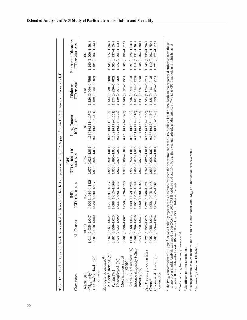
50
Extended Analysis of ACS Study of Particulate Air Pollution and Mortality
Tabl
e 15
.H
Rs
by C
ause
of
Dea
th A
ssoc
iate
d w
ith
an
In
terd
ecil
e C
omp
aris
on V
alu
e of
1.5
µg/
m3 f
rom
th
e 28
-Cou
nty
3-Y
ear
Mod
ela
Cov
aria
tes
All
Cau
ses
IHD
ICD
-9: 4
10–4
14
CP
DIC
D-9
: 400
–440
, 46
0–51
9L
un
g C
ance
rIC
D-9
: 162
Dia
bete
s
ICD
-9: 2
50E
nd
ocri
ne
Dis
ord
ers
ICD
-9: 2
40–2
79
Dea
ths
(n)
10,5
592,
735
4,62
585
311
820
6P
M2.
5 on
lyb
1.01
1 (0
.935
–1.0
47)
1.10
9 (1
.039
–1.1
82)c
0.97
7 (0
.926
–1.0
31)
1.03
6 (0
.911
–1.1
79)
1.32
6 (0
.999
–1.7
59)
1.24
9 (1
.000
–1.5
61)
+ 4
4 In
div
idu
al-l
evel
co
vari
ates
0.98
4 (0
.948
–1.0
20)
1.07
2 (1
.003
–1.1
47)
0.95
3 (0
.902
–1.0
07)
0.95
5 (0
.836
–1.0
91)
1.32
9 (0
.983
–1.7
97)
1.22
4 (0
.965
–1.5
52)
Eco
logi
c co
vari
ates
d
Air
con
dit
ion
ing
(%)
0.98
7 (0
.951
–1.0
24)
1.07
1 (1
.001
–1.1
47)
0.95
6 (0
.904
–1.0
11)
0.96
2 (0
.841
–1.1
02)
1.33
2 (0
.980
–1.8
09)
1.23
5 (0
.973
–1.5
67)
Wh
ite
(%)
0.98
7 (0
.950
–1.0
26)
1.08
8 (1
.013
–1.1
69)
0.95
0 (0
.895
–1.0
08)
1.00
2 (0
.872
–1.1
51)
1.27
3 (0
.920
–1.7
62)
1.20
6 (0
.937
–1.5
54)
Un
emp
loye
d (
%)
0.97
0 (0
.933
–1.0
09)
1.06
6 (0
.992
–1.1
46)
0.92
7 (0
.874
–0.9
84)
0.96
2 (0
.835
–1.1
08)
1.23
9 (0
.891
–1.7
23)
1.17
2 (0
.905
–1.5
18)
Med
ian
hou
seh
old
in
com
e ($
000’
s)0.
968
(0.9
30–1
.007
)1.
050
(0.9
76–1
.130
)0.
922
(0.8
68–0
.979
)0.
950
(0.8
24–1
.095
)1.
249
(0.8
92–1
.751
)1.
165
(0.8
95–1
.517
)
Gra
de
12 e
du
cati
on (
%)
1.00
6 (0
.968
–1.0
45)
1.13
9 (1
.059
–1.2
24)
0.98
3 (0
.927
–1.0
42)
0.98
6 (0
.858
–1.1
35)
1.23
6 (0
.892
–1.7
14)
1.19
1 (0
.923
–1.5
37)
Inco
me
dis
par
ity
(Gin
i)0.
998
(0.9
59–1
.039
)1.
102
(1.0
23–1
.188
)0.
969
(0.9
12–1
.029
)0.
961
(0.8
32–1
.110
)1.
293
(0.9
18–1
.823
)1.
218
(0.9
33–1
.591
)P
over
ty (
%)
0.97
9 (0
.940
–1.0
21)
1.08
0 (1
.000
–1.1
65)
0.92
9 (0
.873
–0.9
90)
1.00
4 (0
.866
–1.1
63)
1.24
7 (0
.875
–1.7
78)
1.18
8 (0
.902
–1.5
65)
All
7 e
colo
gic
cova
riat
es0.
977
(0.9
32–1
.025
)1.
072
(0.9
80–1
.172
)0.
940
(0.8
75–1
.011
)0.
985
(0.8
32–1
.166
)1.
083
(0.7
23–1
.621
)1.
143
(0.8
35–1
.564
)O
zon
ee0.
997
(0.9
55–1
.042
)1.
058
(0.9
75–1
.148
)0.
963
(0.9
02–1
.029
)0.
967
(0.8
28–1
.129
)1.
325
(0.9
18–1
.912
)1.
319
(0.9
92–1
.754
)O
zon
e +
all
7 e
colo
gic
cova
riat
es0.
982
(0.9
34–1
.034
)1.
054
(0.9
57–1
.161
)0.
938
(0.8
68–1
.014
)1.
000
(0.8
36–1
.196
)1.
099
(0.7
05–1
.711
)1.
221
(0.8
71–1
.712
)
a T
he
PM
2.5
con
cen
trat
ion
of
1.5
µg/
m3
for
New
Yor
k C
ity
rep
rese
nts
th
e d
iffe
ren
ce b
etw
een
th
e co
nce
ntr
atio
ns
at t
he
90%
dec
ile
and
at
the
10%
dec
ile
in t
he
exp
osu
re d
istr
ibu
tion
fro
m t
he
28-
cou
nty
3-y
ear
mod
el. A
nal
ysis
was
bas
ed o
n 7
46 Z
CA
s w
ith
AC
S C
PS
-II
resi
den
ts a
nd
str
atif
ied
by
age
(in
1-y
ear
grou
pin
gs),
gen
der
, an
d r
ace.
N =
44,
056
CP
S-I
I p
arti
cip
ants
liv
ing
in t
he
28
cou
nti
es. B
old
ed d
ata
refe
r to
tex
t. H
Rs
are
foll
owed
by
95%
con
fid
ence
in
terv
als.
b Pre
dic
ted
usi
ng
the
28-c
oun
ty 3
-yea
r m
odel
.c S
ign
ific
ant
pos
itiv
e as
soci
atio
n.
d E
colo
gic
cova
riat
es w
ere
incl
ud
ed o
ne
at a
tim
e to
a b
ase
mod
el w
ith
PM
2.5
+ 4
4 in
div
idu
al-l
evel
cov
aria
tes.
e S
um
mer
O3
valu
es f
or 1
999–
2001
.
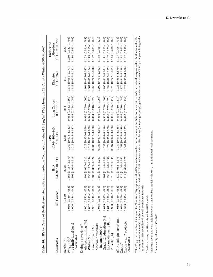
D. Krewski et al.
51
Tabl
e 1
6.H
Rs
by C
ause
of
Dea
th A
ssoc
iate
d w
ith
an
In
terd
ecil
e C
omp
aris
on V
alu
e of
3.9
µg/
m3 P
M2.
5 fr
om t
he
28-C
oun
ty W
inte
r-20
00 M
odel
a
Cov
aria
tes
All
Cau
ses
IHD
ICD
-9: 4
10–4
14
CP
DIC
D-9
: 400
–440
, 46
0–51
9L
un
g C
ance
rIC
D-9
: 162
Dia
bete
s
ICD
-9: 2
50
En
doc
rin
e D
isor
der
sIC
D-9
: 240
–279
Dea
ths
(n)
10,5
592,
735
4,62
585
311
820
6P
M2.
5 on
lyb
1.03
6 (0
.989
–1.0
85)
1.26
3 (1
.157
–1.3
79)
1.04
7 (0
.978
–1.1
22)
0.98
4 (0
.832
–1.1
64)
1.47
6 (0
.959
–2.2
71)
1.28
9 (0
.927
–1.7
93)
+ 4
4 In
div
idu
al-l
evel
co
vari
ates
1.00
0 (0
.954
–1.0
48)
1.20
3 (1
.099
–1.3
16)
1.01
3 (0
.945
–1.0
87)
0.89
3 (0
.754
–1.0
58)
1.42
3 (0
.907
–2.2
32)
1.21
4 (0
.863
–1.7
08)
Eco
logi
c co
vari
ates
c
Air
con
dit
ion
ing
(%)
1.00
1 (0
.953
–1.0
52)
1.19
4 (1
.087
–1.3
12)
1.02
2 (0
.950
–1.0
99)
0.88
6 (0
.739
–1.0
63)
1.40
4 (0
.878
–2.2
47)
1.25
3 (0
.881
–1.7
81)
Wh
ite
(%)
1.00
2 (0
.953
–1.0
53)
1.23
0 (1
.117
–1.3
54)
1.01
1 (0
.938
–1.0
89)
0.94
1 (0
.786
–1.1
26)
1.30
7 (0
.805
–2.1
24)
1.17
3 (0
.815
–1.6
88)
Un
emp
loye
d (
%)
0.98
1 (0
.933
–1.0
32)
1.20
0 (1
.089
–1.3
22)
0.98
3 (0
.912
–1.0
60)
0.89
4 (0
.746
–1.0
72)
1.25
8 (0
.772
–2.0
50)
1.12
7 (0
.781
–1.6
28)
Med
ian
hou
seh
old
in
com
e ($
000’
s)0.
985
(0.9
38–1
.035
)1.
180
(1.0
73–1
.297
)0.
986
(0.9
17–1
.061
)0.
891
(0.7
47–1
.063
)1.
290
(0.7
99–2
.082
)1.
138
(0.7
96–1
.629
)
Gra
de
12 e
du
cati
on (
%)
1.01
5 (0
.967
–1.0
66)
1.26
1 (1
.148
–1.3
86)
1.03
7 (0
.964
–1.1
16)
0.91
7 (0
.769
–1.0
92)
1.29
5 (0
.810
–2.0
71)
1.17
1 (0
.822
–1.6
68)
Inco
me
dis
par
ity
(Gin
i)1.
011
(0.9
62–1
.062
)1.
233
(1.1
20–1
.358
)1.
029
(0.9
55–1
.109
)0.
898
(0.7
52–1
.073
)1.
332
(0.8
22–2
.157
)1.
182
(0.8
23–1
.697
)P
over
ty (
%)
0.99
6 (0
.946
–1.0
47)
1.21
6 (1
.102
–1.3
41)
0.99
7 (0
.924
–1.0
76)
0.93
0 (0
.775
–1.1
17)
1.27
0 (0
.772
–2.0
91)
1.14
4 (0
.788
–1.6
60)
All
7 e
colo
gic
cova
riat
es0.
989
(0.9
29–1
.054
)1.
220
(1.0
82–1
.375
)1.
034
(0.9
41–1
.135
)0.
891
(0.7
10–1
.117
)1.
026
(0.5
63–1
.870
)1.
107
(0.7
06–1
.736
)O
zon
ed1.
024
(0.9
70–1
.082
)1.
224
(1.1
00–1
.362
)1.
058
(0.9
74–1
.148
)0.
892
(0.7
36–1
.082
)1.
376
(0.8
16–2
.318
)1.
282
(0.8
63–1
.905
)O
zon
e +
all
7 e
colo
gic
cova
riat
es0.
999
(0.9
35–1
.068
)1.
212
(1.0
66–1
.377
)1.
047
(0.9
48–1
.157
)0.
897
(0.7
07–1
.139
)1.
028
(0.5
39–1
.960
)1.
182
(0.7
32–1
.909
)
a Th
e P
M2.
5 co
nce
ntr
atio
n o
f 3.
9 µ
g/m
3 for
New
Yor
k C
ity
rep
rese
nts
th
e d
iffe
ren
ce b
etw
een
th
e co
nce
ntr
atio
ns
at t
he
90%
dec
ile
and
at
the
10%
dec
ile
in t
he
exp
osu
re d
istr
ibu
tion
fro
m t
he
28-
cou
nty
win
ter-
2000
mod
el. A
nal
ysis
was
bas
ed o
n 7
46 Z
CA
s w
ith
AC
S C
PS
-II
resi
den
ts a
nd
str
atif
ied
by
age
(in
1-y
ear
grou
pin
gs),
gen
der
, an
d r
ace.
N =
44,
056
CP
S-I
I p
arti
cip
ants
liv
ing
in t
he
28 c
oun
ties
. HR
s ar
e fo
llow
ed b
y 95
% c
onfi
den
ce i
nte
rval
s.b P
red
icte
d u
sin
g th
e 28
-cou
nty
win
ter-
2000
mod
el.
c E
colo
gic
cova
riat
es w
ere
incl
ud
ed o
ne
at a
tim
e to
a b
ase
mod
el w
ith
PM
2.5
+ 4
4 in
div
idu
al-l
evel
cov
aria
tes.
d S
um
mer
O3
valu
es f
or 1
999–
2001
.
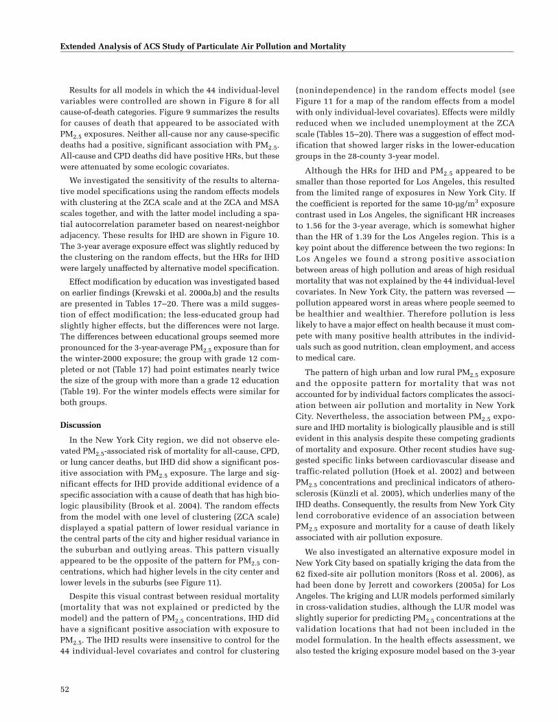
52
Extended Analysis of ACS Study of Particulate Air Pollution and Mortality
Results for all models in which the 44 individual-levelvariables were controlled are shown in Figure 8 for allcause-of-death categories. Figure 9 summarizes the resultsfor causes of death that appeared to be associated withPM2.5 exposures. Neither all-cause nor any cause-specificdeaths had a positive, significant association with PM2.5.All-cause and CPD deaths did have positive HRs, but thesewere attenuated by some ecologic covariates.
We investigated the sensitivity of the results to alterna-tive model specifications using the random effects modelswith clustering at the ZCA scale and at the ZCA and MSAscales together, and with the latter model including a spa-tial autocorrelation parameter based on nearest-neighboradjacency. These results for IHD are shown in Figure 10.The 3-year average exposure effect was slightly reduced bythe clustering on the random effects, but the HRs for IHDwere largely unaffected by alternative model specification.
Effect modification by education was investigated basedon earlier findings (Krewski et al. 2000a,b) and the resultsare presented in Tables 17–20. There was a mild sugges-tion of effect modification; the less-educated group hadslightly higher effects, but the differences were not large.The differences between educational groups seemed morepronounced for the 3-year-average PM2.5 exposure than forthe winter-2000 exposure; the group with grade 12 com-pleted or not (Table 17) had point estimates nearly twicethe size of the group with more than a grade 12 education(Table 19). For the winter models effects were similar forboth groups.
Discussion
In the New York City region, we did not observe ele-vated PM2.5-associated risk of mortality for all-cause, CPD,or lung cancer deaths, but IHD did show a significant pos-itive association with PM2.5 exposure. The large and sig-nificant effects for IHD provide additional evidence of aspecific association with a cause of death that has high bio-logic plausibility (Brook et al. 2004). The random effectsfrom the model with one level of clustering (ZCA scale)displayed a spatial pattern of lower residual variance inthe central parts of the city and higher residual variance inthe suburban and outlying areas. This pattern visuallyappeared to be the opposite of the pattern for PM2.5 con-centrations, which had higher levels in the city center andlower levels in the suburbs (see Figure 11).
Despite this visual contrast between residual mortality(mortality that was not explained or predicted by themodel) and the pattern of PM2.5 concentrations, IHD didhave a significant positive association with exposure toPM2.5. The IHD results were insensitive to control for the44 individual-level covariates and control for clustering
(nonindependence) in the random effects model (seeFigure 11 for a map of the random effects from a modelwith only individual-level covariates). Effects were mildlyreduced when we included unemployment at the ZCAscale (Tables 15–20). There was a suggestion of effect mod-ification that showed larger risks in the lower-educationgroups in the 28-county 3-year model.
Although the HRs for IHD and PM2.5 appeared to besmaller than those reported for Los Angeles, this resultedfrom the limited range of exposures in New York City. Ifthe coefficient is reported for the same 10-µg/m3 exposurecontrast used in Los Angeles, the significant HR increasesto 1.56 for the 3-year average, which is somewhat higherthan the HR of 1.39 for the Los Angeles region. This is akey point about the difference between the two regions: InLos Angeles we found a strong positive associationbetween areas of high pollution and areas of high residualmortality that was not explained by the 44 individual-levelcovariates. In New York City, the pattern was reversed —pollution appeared worst in areas where people seemed tobe healthier and wealthier. Therefore pollution is lesslikely to have a major effect on health because it must com-pete with many positive health attributes in the individ-uals such as good nutrition, clean employment, and accessto medical care.
The pattern of high urban and low rural PM2.5 exposureand the opposite pattern for mortality that was notaccounted for by individual factors complicates the associ-ation between air pollution and mortality in New YorkCity. Nevertheless, the association between PM2.5 expo-sure and IHD mortality is biologically plausible and is stillevident in this analysis despite these competing gradientsof mortality and exposure. Other recent studies have sug-gested specific links between cardiovascular disease andtraffic-related pollution (Hoek et al. 2002) and betweenPM2.5 concentrations and preclinical indicators of athero-sclerosis (Künzli et al. 2005), which underlies many of theIHD deaths. Consequently, the results from New York Citylend corroborative evidence of an association betweenPM2.5 exposure and mortality for a cause of death likelyassociated with air pollution exposure.
We also investigated an alternative exposure model inNew York City based on spatially kriging the data from the62 fixed-site air pollution monitors (Ross et al. 2006), ashad been done by Jerrett and coworkers (2005a) for LosAngeles. The kriging and LUR models performed similarlyin cross-validation studies, although the LUR model wasslightly superior for predicting PM2.5 concentrations at thevalidation locations that had not been included in themodel formulation. In the health effects assessment, wealso tested the kriging exposure model based on the 3-year

D. Krewski et al.
53
Figure 8. HRs by cause of death associated with an interdecile comparison value of 1.5 µg/m3 PM2.5 from the 28-county 3-year model and 3.9 µg/m3 PM2.5from the winter-2000 model. Analysis was based on 746 ZCAs with ACS CPS-II residents and stratified by age (in 1-year groupings), gender, and race. N =44,056 participants living in the 28 counties; number of deaths for each cause is given beneath the ICD-9 codes. (See also Tables 15 and 16.)
Figure 9. HRs by selected causes of death associated with an interdecilecomparison value of 1.5 µg/m3 PM2.5 from the 28-county 3-year modeland 3.9 µg/m3 PM2.5 from the winter-2000 model. Analysis was based on746 ZCAs with ACS CPS-II residents and stratified by age (in 1-yeargroupings), gender, and race. N = 44,056 participants living in the 28counties; number of deaths for each cause is given beneath the ICD-9codes. (See also Tables 15 and 16.)
Figure 10. HR results for IHD deaths from analyses with one (ZCA) or two(ZCA and MSA) levels of clustering and with or without � (a statisticalestimate of the homogeneity of PM2.5 exposure within a cluster). Deathswere associated with an interdecile comparison value of 1.5 µg/m3 PM2.5from the 28-county 3-year model and 3.9 µg/m3 PM2.5 from the winter-2000model. Analysis was based on 746 ZCAs with ACS CPS-II residents andwas stratified by age (in 1-year groupings), gender, and race.
average PM2.5 concentrations. Risk estimates were similar tobut slightly smaller than those obtained with the LUR model.Because of concerns about attenuation of risk estimates dueto exposure measurement error with spatial kriging, we
based our risk estimates on LUR. This suggests that differ-ences in results between the New York City and Los AngelesAnalyses (see the next section) are likely not due to differentmethods used to ascertain levels of exposures.
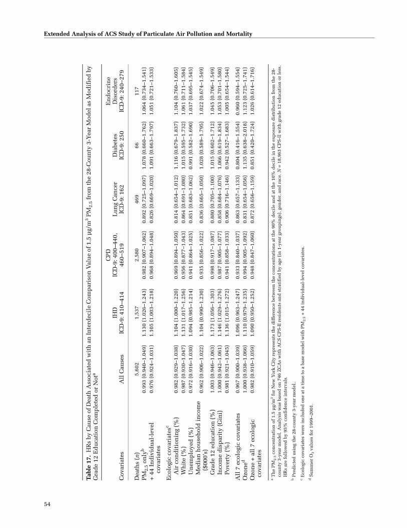
54
Extended Analysis of ACS Study of Particulate Air Pollution and Mortality
Tabl
e 17
.H
Rs
by C
ause
of D
eath
Ass
ocia
ted
wit
h a
n In
terd
ecil
e C
omp
aris
on V
alu
e of
1.5
µg/
m3 P
M2.
5 fr
om t
he
28-C
oun
ty 3
-Yea
r M
odel
as
Mod
ifie
d b
y G
rad
e 12
Ed
uca
tion
Com
ple
ted
or
Not
a
Cov
aria
tes
All
Cau
ses
IHD
ICD
-9: 4
10–4
14
CP
DIC
D-9
: 400
–440
, 46
0–51
9L
un
g C
ance
rIC
D-9
: 162
Dia
bete
sIC
D-9
: 250
En
doc
rin
e D
isor
der
sIC
D-9
: 240
–279
Dea
ths
(n)
5,60
21,
537
2,58
046
966
117
PM
2.5
only
b0.
993
(0.9
40–1
.049
)1.
130
(1.0
26–1
.243
)0.
982
(0.9
07–1
.062
)0.
892
(0.7
25–1
.097
)1.
078
(0.6
60–1
.762
)1.
064
(0.7
34–1
.541
)+
44
Ind
ivid
ual
-lev
el
cova
riat
es0.
976
(0.9
24–1
.031
)1.
105
(1.0
03–1
.218
)0.
968
(0.8
94–1
.048
)0.
826
(0.6
69–1
.020
)1.
091
(0.6
63–1
.797
)1.
051
(0.7
21–1
.533
)
Eco
logi
c co
vari
ates
c
Air
con
dit
ion
ing
(%)
0.98
2 (0
.929
–1.0
38)
1.10
4 (1
.000
–1.2
20)
0.96
9 (0
.894
–1.0
50)
0.81
4 (0
.654
–1.0
12)
1.11
6 (0
.679
–1.8
37)
1.10
4 (0
.760
–1.6
05)
Wh
ite
(%)
0.98
7 (0
.930
–1.0
47)
1.13
1 (1
.017
–1.2
56)
0.95
6 (0
.877
–1.0
43)
0.86
4 (0
.691
–1.0
80)
1.01
5 (0
.595
–1.7
32)
1.06
1 (0
.711
–1.5
84)
Un
emp
loye
d (
%)
0.97
2 (0
.916
–1.0
30)
1.09
4 (0
.985
–1.2
14)
0.94
1 (0
.864
–1.0
25)
0.85
1 (0
.683
–1.0
62)
0.99
1 (0
.582
–1.6
90)
1.03
7 (0
.695
–1.5
45)
Med
ian
hou
seh
old
in
com
e ($
000’
s)0.
962
(0.9
06–1
.022
)1.
104
(0.9
90–1
.230
)0.
935
(0.8
56–1
.022
)0.
836
(0.6
65–1
.050
)1.
028
(0.5
89–1
.795
)1.
022
(0.6
74–1
.549
)
Gra
de
12 e
du
cati
on (
%)
1.00
3 (0
.946
–1.0
63)
1.17
3 (1
.056
–1.3
03)
0.99
8 (0
.917
–1.0
87)
0.88
0 (0
.705
–1.1
00)
1.01
5 (0
.602
–1.7
12)
1.04
5 (0
.706
–1.5
49)
Inco
me
dis
par
ity
(Gin
i)1.
000
(0.9
42–1
.061
)1.
146
(1.0
29–1
.276
)0.
987
(0.9
05–1
.077
)0.
858
(0.6
84–1
.076
)1.
066
(0.6
19–1
.834
)1.
053
(0.7
01–1
.580
)P
over
ty (
%)
0.98
1 (0
.921
–1.0
45)
1.13
6 (1
.015
–1.2
72)
0.94
1 (0
.858
–1.0
33)
0.90
6 (0
.716
–1.1
46)
0.94
2 (0
.527
–1.6
83)
1.00
5 (0
.654
–1.5
44)
All
7 e
colo
gic
cova
riat
es0.
967
(0.9
00–1
.039
)1.
096
(0.9
63–1
.247
)0.
933
(0.8
40–1
.037
)0.
863
(0.6
57–1
.133
)0.
804
(0.4
16–1
.554
)0.
960
(0.5
94–1
.554
)O
zon
ed1.
000
(0.9
38–1
.066
)1.
110
(0.9
79–1
.235
)0.
994
(0.9
05–1
.092
)0.
831
(0.6
54–1
.056
)1.
135
(0.6
38–2
.018
)1.
123
(0.7
25–1
.741
)O
zon
e +
all
7 e
colo
gic
cova
riat
es0.
982
(0.9
10–1
.059
)1.
090
(0.9
50–1
.252
)0.
948
(0.8
47–1
.060
)0.
872
(0.6
56–1
.159
)0.
851
(0.4
20–1
.724
)1.
026
(0.6
14–1
.716
)
a Th
e P
M2.
5 co
nce
ntr
atio
n o
f 1.
5 µ
g/m
3 for
New
Yor
k C
ity
rep
rese
nts
th
e d
iffe
ren
ce b
etw
een
th
e co
nce
ntr
atio
ns
at t
he
90%
dec
ile
and
at
the
10%
dec
ile
in t
he
exp
osu
re d
istr
ibu
tion
fro
m t
he
28-
cou
nty
3-y
ear
mod
el. A
nal
ysis
was
bas
ed o
n 7
46 Z
CA
s w
ith
AC
S C
PS
-II
resi
den
ts a
nd
str
atif
ied
by
age
(in
1-y
ear
grou
pin
gs),
gen
der
, an
d r
ace.
N =
18,
963
CP
S-I
I w
ith
gra
de
12 e
du
cati
on o
r le
ss.
HR
s ar
e fo
llow
ed b
y 95
% c
onfi
den
ce i
nte
rval
s.b P
red
icte
d u
sin
g th
e 28
-cou
nty
3-y
ear
mod
el.
c E
colo
gic
cova
riat
es w
ere
incl
ud
ed o
ne
at a
tim
e to
a b
ase
mod
el w
ith
PM
2.5
+ 4
4 in
div
idu
al-l
evel
cov
aria
tes.
d S
um
mer
O3
valu
es f
or 1
999–
2001
.
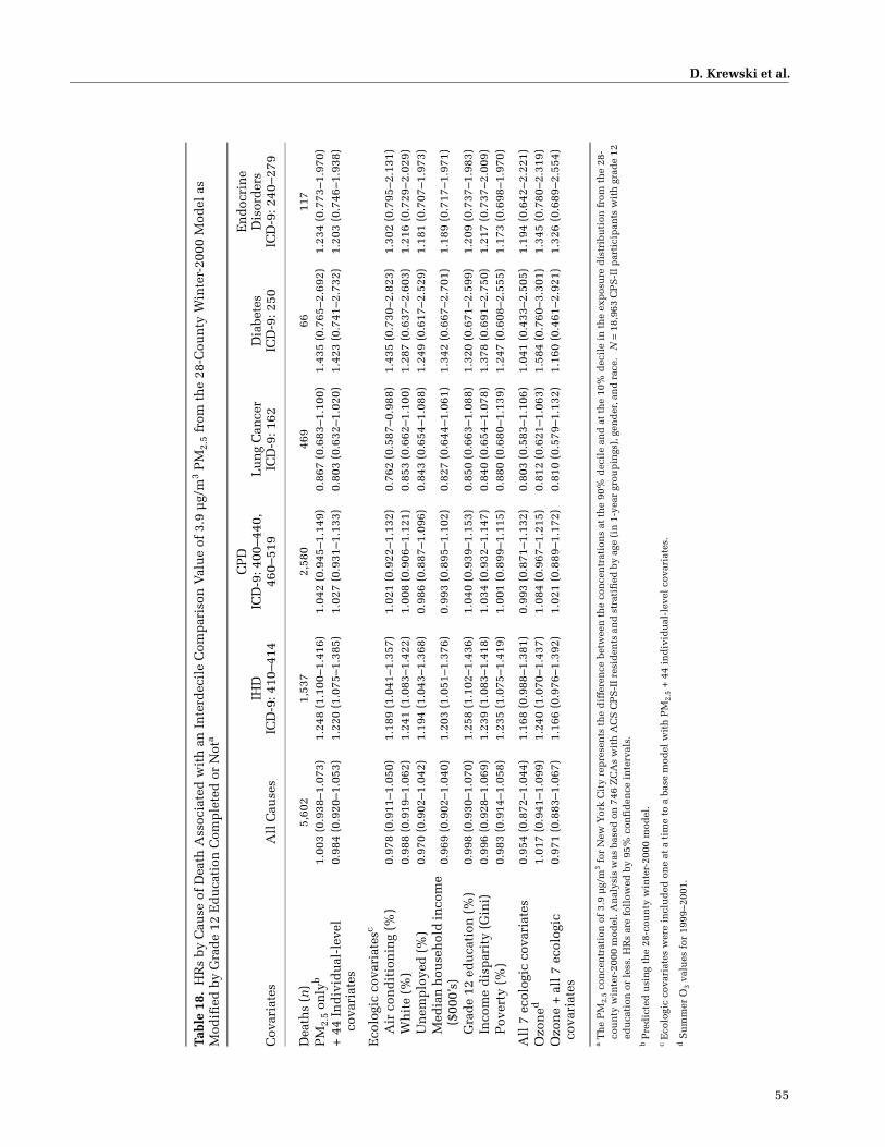
D. Krewski et al.
55
Tabl
e 18
.H
Rs
by C
ause
of
Dea
th A
ssoc
iate
d w
ith
an
In
terd
ecil
e C
omp
aris
on V
alu
e of
3.9
µg/
m3 P
M2.
5 fr
om t
he
28-C
oun
ty W
inte
r-20
00 M
odel
as
Mod
ifie
d b
y G
rad
e 12
Ed
uca
tion
Com
ple
ted
or
Not
a
Cov
aria
tes
All
Cau
ses
IHD
ICD
-9: 4
10–4
14
CP
DIC
D-9
: 400
–440
, 46
0–51
9L
un
g C
ance
rIC
D-9
: 162
Dia
bete
sIC
D-9
: 250
En
doc
rin
eD
isor
der
sIC
D-9
: 240
–279
Dea
ths
(n)
5,60
21,
537
2,58
046
966
117
PM
2.5
only
b1.
003
(0.9
38–1
.073
)1.
248
(1.1
00–1
.416
)1.
042
(0.9
45–1
.149
)0.
867
(0.6
83–1
.100
)1.
435
(0.7
65–2
.692
)1.
234
(0.7
73–1
.970
)+
44
Ind
ivid
ual
-lev
el
cova
riat
es0.
984
(0.9
20–1
.053
)1.
220
(1.0
75–1
.385
)1.
027
(0.9
31–1
.133
)0.
803
(0.6
32–1
.020
)1.
423
(0.7
41–2
.732
)1.
203
(0.7
46–1
.938
)
Eco
logi
c co
vari
ates
c
Air
con
dit
ion
ing
(%)
0.97
8 (0
.911
–1.0
50)
1.18
9 (1
.041
–1.3
57)
1.02
1 (0
.922
–1.1
32)
0.76
2 (0
.587
–0.9
88)
1.43
5 (0
.730
–2.8
23)
1.30
2 (0
.795
–2.1
31)
Wh
ite
(%)
0.98
8 (0
.919
–1.0
62)
1.24
1 (1
.083
–1.4
22)
1.00
8 (0
.906
–1.1
21)
0.85
3 (0
.662
–1.1
00)
1.28
7 (0
.637
–2.6
03)
1.21
6 (0
.729
–2.0
29)
Un
emp
loye
d (
%)
0.97
0 (0
.902
–1.0
42)
1.19
4 (1
.043
–1.3
68)
0.98
6 (0
.887
–1.0
96)
0.84
3 (0
.654
–1.0
88)
1.24
9 (0
.617
–2.5
29)
1.18
1 (0
.707
–1.9
73)
Med
ian
hou
seh
old
inco
me
($00
0’s)
0.96
9 (0
.902
–1.0
40)
1.20
3 (1
.051
–1.3
76)
0.99
3 (0
.895
–1.1
02)
0.82
7 (0
.644
–1.0
61)
1.34
2 (0
.667
–2.7
01)
1.18
9 (0
.717
–1.9
71)
Gra
de
12 e
du
cati
on (
%)
0.99
8 (0
.930
–1.0
70)
1.25
8 (1
.102
–1.4
36)
1.04
0 (0
.939
–1.1
53)
0.85
0 (0
.663
–1.0
88)
1.32
0 (0
.671
–2.5
99)
1.20
9 (0
.737
–1.9
83)
Inco
me
dis
par
ity
(Gin
i)0.
996
(0.9
28–1
.069
)1.
239
(1.0
83–1
.418
)1.
034
(0.9
32–1
.147
)0.
840
(0.6
54–1
.078
)1.
378
(0.6
91–2
.750
)1.
217
(0.7
37–2
.009
)P
over
ty (
%)
0.98
3 (0
.914
–1.0
58)
1.23
5 (1
.075
–1.4
19)
1.00
1 (0
.899
–1.1
15)
0.88
0 (0
.680
–1.1
39)
1.24
7 (0
.608
–2.5
55)
1.17
3 (0
.698
–1.9
70)
All
7 e
colo
gic
cova
riat
es0.
954
(0.8
72–1
.044
)1.
168
(0.9
88–1
.381
)0.
993
(0.8
71–1
.132
)0.
803
(0.5
83–1
.106
)1.
041
(0.4
33–2
.505
)1.
194
(0.6
42–2
.221
)O
zon
ed1.
017
(0.9
41–1
.099
)1.
240
(1.0
70–1
.437
)1.
084
(0.9
67–1
.215
)0.
812
(0.6
21–1
.063
)1.
584
(0.7
60–3
.301
)1.
345
(0.7
80–2
.319
)O
zon
e +
all
7 e
colo
gic
cova
riat
es0.
971
(0.8
83–1
.067
)1.
166
(0.9
76–1
.392
)1.
021
(0.8
89–1
.172
)0.
810
(0.5
79–1
.132
)1.
160
(0.4
61–2
.921
)1.
326
(0.6
89–2
.554
)
a Th
e P
M2.
5 co
nce
ntr
atio
n o
f 3.
9 µ
g/m
3 for
New
Yor
k C
ity
rep
rese
nts
th
e d
iffe
ren
ce b
etw
een
th
e co
nce
ntr
atio
ns
at t
he
90%
dec
ile
and
at
the
10%
dec
ile
in t
he
exp
osu
re d
istr
ibu
tion
fro
m t
he
28-
cou
nty
win
ter-
2000
mod
el. A
nal
ysis
was
bas
ed o
n 7
46 Z
CA
s w
ith
AC
S C
PS
-II r
esid
ents
an
d s
trat
ifie
d b
y ag
e (i
n 1
-yea
r gr
oup
ings
), g
end
er, a
nd
rac
e.
N =
18,
963
CP
S-I
I par
tici
pan
ts w
ith
gra
de
12
edu
cati
on o
r le
ss. H
Rs
are
foll
owed
by
95%
con
fid
ence
in
terv
als.
b Pre
dic
ted
usi
ng
the
28-c
oun
ty w
inte
r-20
00 m
odel
.c
Eco
logi
c co
vari
ates
wer
e in
clu
ded
on
e at
a t
ime
to a
bas
e m
odel
wit
h P
M2.
5 +
44
ind
ivid
ual
-lev
el c
ovar
iate
s.
d S
um
mer
O3
valu
es f
or 1
999–
2001
.

56
Extended Analysis of ACS Study of Particulate Air Pollution and Mortality
Tabl
e 19
.H
Rs
by C
ause
of
Dea
th A
ssoc
iate
d w
ith
an
In
terd
ecil
e C
omp
aris
on V
alu
e of
1.5
µg/
m3 P
M2.
5 fr
om t
he
28-C
oun
ty 3
-Yea
r M
odel
as
Mod
ifie
d b
y M
ore
Th
an G
rad
e 12
Ed
uca
tion
a
Cov
aria
tes
All
Cau
ses
IHD
ICD
-9: 4
10–4
14
CP
DIC
D-9
: 400
–440
, 46
0–51
9L
un
g C
ance
rIC
D-9
: 162
Dia
bete
sIC
D-9
: 250
En
doc
rin
eD
isor
der
sIC
D-9
: 240
–279
Dea
ths
(n)
4,95
71,
198
2,04
538
452
89P
M2.
5 on
lyb
1.02
2 (0
.974
–1.0
72)
1.08
9 (0
.993
–1.1
95)
0.96
4 (0
.892
–1.0
41)
1.12
1 (0
.949
–1.3
24)
1.60
8 (1
.134
–2.2
82)
1.49
0 (1
.121
–1.9
79)
+ 4
4 In
div
idu
al-l
evel
co
vari
ates
0.98
6 (0
.938
–1.0
36)
1.03
2 (0
.937
–1.1
36)
0.92
4 (0
.854
–1.0
00)
1.05
5 (0
.891
–1.2
50)
1.41
1 (0
.959
–2.0
77)
1.39
3 (1
.026
–1.8
93)
Eco
logi
c co
vari
ates
c
Air
con
dit
ion
ing
(%)
0.98
8 (0
.940
–1.0
39)
1.03
8 (0
.943
–1.1
44)
0.93
0 (0
.859
–1.0
08)
1.08
0 (0
.910
–1.2
82)
1.32
6 (0
.884
–1.9
89)
1.36
3 (0
.997
–1.8
63)
Wh
ite
(%)
0.98
5 (0
.935
–1.0
38)
1.04
4 (0
.943
–1.1
55)
0.93
1 (0
.857
–1.0
13)
1.09
5 (0
.917
–1.3
06)
1.22
5 (0
.791
–1.8
98)
1.27
1 (0
.905
–1.7
85)
Un
emp
loye
d (
%)
0.96
4 (0
.913
–1.0
17)
1.03
4 (0
.932
–1.1
47)
0.90
1 (0
.827
–0.9
81)
1.03
7 (0
.862
–1.2
47)
1.18
3 (0
.746
–1.8
73)
1.27
5 (0
.898
–1.8
10)
Med
ian
hou
seh
old
inco
me
($00
0’s)
0.96
8 (0
.919
–1.0
21)
1.00
4 (0
.906
–1.1
12)
0.89
8 (0
.825
–0.9
77)
1.04
4 (0
.871
–1.2
51)
1.22
7 (0
.791
–1.9
04)
1.25
5 (0
.888
–1.7
74)
Gra
de
12 e
du
cati
on (
%)
1.00
0 (0
.950
–1.0
54)
1.09
4 (0
.987
–1.2
12)
0.94
9 (0
.873
–1.0
31)
1.05
4 (0
.883
–1.2
59)
1.22
9 (0
.791
–1.9
10)
1.30
2 (0
.929
–1.8
24)
Inco
me
dis
par
ity
(Gin
i)0.
989
(0.9
37–1
.045
)1.
052
(0.9
45–1
.171
)0.
935
(0.8
56–1
.020
)1.
014
(0.8
41–1
.223
)1.
288
(0.8
03–2
.067
)1.
307
(0.9
08–1
.882
)P
over
ty (
%)
0.96
6 (0
.913
–1.0
21)
1.01
3 (0
.909
–1.1
28)
0.90
0 (0
.823
–0.9
84)
1.05
5 (0
.873
–1.2
75)
1.20
0 (0
.748
–1.9
27)
1.23
3 (0
.852
–1.7
84)
All
7 e
colo
gic
cova
riat
es0.
968
(0.9
07–1
.034
)1.
036
(0.9
09–1
.181
)0.
923
(0.8
31–1
.024
)0.
998
(0.7
99–1
.247
)1.
040
(0.5
77–1
.875
)1.
243
(0.8
04–1
.921
)O
zon
ed0.
982
(0.9
25–1
.043
)1.
001
(0.8
89–1
.127
)0.
910
(0.8
27–1
.002
)1.
060
(0.8
62–1
.304
)1.
268
(0.7
63–2
.108
)1.
414
(0.9
58–2
.087
)O
zon
e +
all
7 e
colo
gic
cova
riat
es0.
959
(0.8
93–1
.029
)0.
998
(0.8
66–1
.151
)0.
895
(0.7
99–1
.003
)1.
020
(0.8
02–1
.298
)0.
940
(0.4
84–1
.827
)1.
257
(0.7
80–2
.024
)
a Th
e P
M2.
5 co
nce
ntr
atio
n o
f 1.
5 µ
g/m
3 for
New
Yor
k C
ity
rep
rese
nts
th
e d
iffe
ren
ce b
etw
een
th
e co
nce
ntr
atio
ns
at t
he
90%
dec
ile
and
at
the
10%
dec
ile
in t
he
exp
osu
re d
istr
ibu
tion
fro
m t
he
28-
cou
nty
3-y
ear
mod
el. A
nal
ysis
was
bas
ed o
n 7
46 Z
CA
s w
ith
AC
S C
PS
-II
resi
den
ts a
nd
str
atif
ied
by
age
(in
1-y
ear
grou
pin
gs),
gen
der
, an
d r
ace.
N =
25,
093
CP
S-I
I p
arti
cip
ants
wit
h m
ore
than
gr
ade
12 e
du
cati
on. H
Rs
are
foll
owed
by
95%
con
fid
ence
in
terv
als.
b Pre
dic
ted
usi
ng
the
28-c
oun
ty 3
-yea
r m
odel
.c
Eco
logi
c co
vari
ates
wer
e in
clu
ded
on
e at
a t
ime
to a
bas
e m
odel
wit
h P
M2.
5 +
44
ind
ivid
ual
-lev
el c
ovar
iate
s.
d S
um
mer
O3
valu
es f
or 1
999–
2001
.
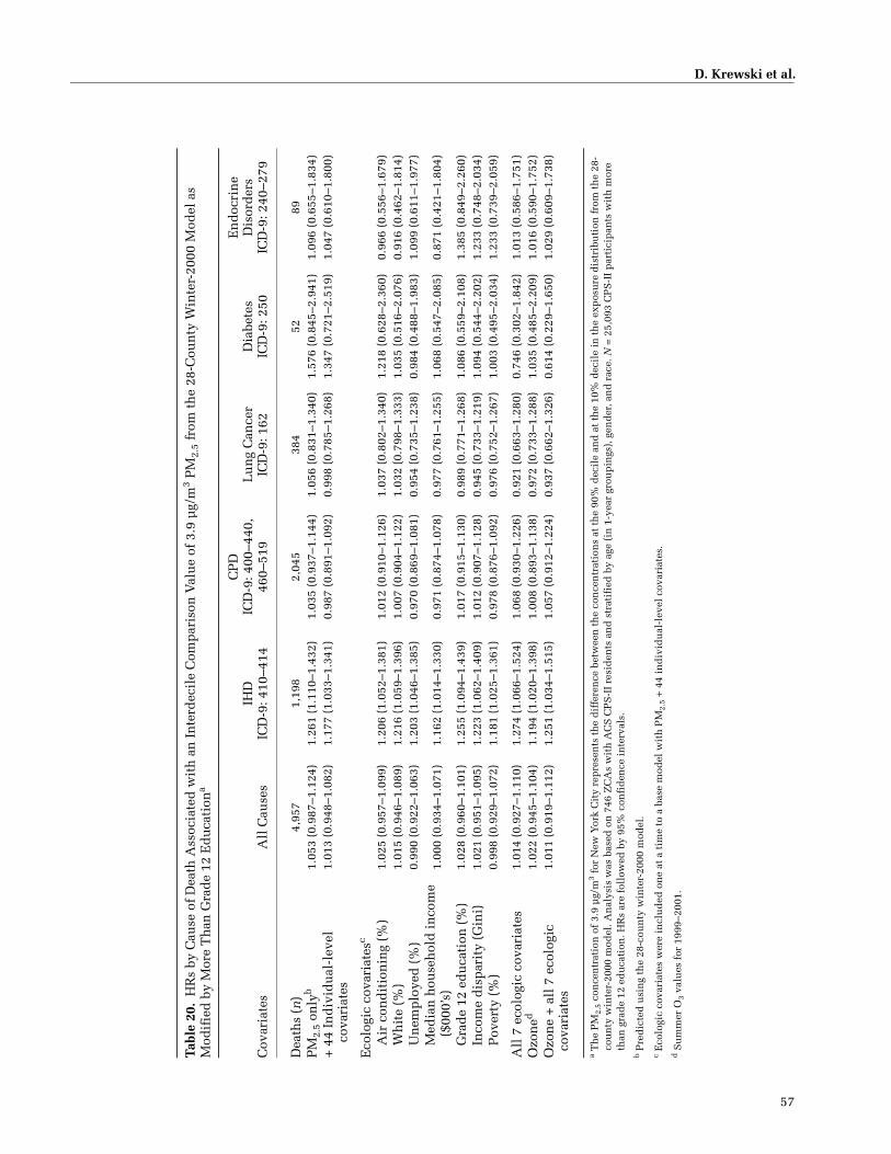
D. Krewski et al.
57
Tabl
e 20
.H
Rs
by C
ause
of
Dea
th A
ssoc
iate
d w
ith
an
In
terd
ecil
e C
omp
aris
on V
alu
e of
3.9
µg/
m3 P
M2.
5 fr
om t
he
28-C
oun
ty W
inte
r-20
00 M
odel
as
Mod
ifie
d b
y M
ore
Th
an G
rad
e 12
Ed
uca
tion
a
Cov
aria
tes
All
Cau
ses
IHD
ICD
-9: 4
10–4
14
CP
DIC
D-9
: 400
–440
, 46
0–51
9L
un
g C
ance
rIC
D-9
: 162
Dia
bete
sIC
D-9
: 250
En
doc
rin
eD
isor
der
sIC
D-9
: 240
–279
Dea
ths
(n)
4,95
71,
198
2,04
538
452
89P
M2.
5 on
lyb
1.05
3 (0
.987
–1.1
24)
1.26
1 (1
.110
–1.4
32)
1.03
5 (0
.937
–1.1
44)
1.05
6 (0
.831
–1.3
40)
1.57
6 (0
.845
–2.9
41)
1.09
6 (0
.655
–1.8
34)
+ 4
4 In
div
idu
al-l
evel
co
vari
ates
1.01
3 (0
.948
–1.0
82)
1.17
7 (1
.033
–1.3
41)
0.98
7 (0
.891
–1.0
92)
0.99
8 (0
.785
–1.2
68)
1.34
7 (0
.721
–2.5
19)
1.04
7 (0
.610
–1.8
00)
Eco
logi
c co
vari
ates
c
Air
con
dit
ion
ing
(%)
1.02
5 (0
.957
–1.0
99)
1.20
6 (1
.052
–1.3
81)
1.01
2 (0
.910
–1.1
26)
1.03
7 (0
.802
–1.3
40)
1.21
8 (0
.628
–2.3
60)
0.96
6 (0
.556
–1.6
79)
Wh
ite
(%)
1.01
5 (0
.946
–1.0
89)
1.21
6 (1
.059
–1.3
96)
1.00
7 (0
.904
–1.1
22)
1.03
2 (0
.798
–1.3
33)
1.03
5 (0
.516
–2.0
76)
0.91
6 (0
.462
–1.8
14)
Un
emp
loye
d (
%)
0.99
0 (0
.922
–1.0
63)
1.20
3 (1
.046
–1.3
85)
0.97
0 (0
.869
–1.0
81)
0.95
4 (0
.735
–1.2
38)
0.98
4 (0
.488
–1.9
83)
1.09
9 (0
.611
–1.9
77)
Med
ian
hou
seh
old
in
com
e ($
000’
s)1.
000
(0.9
34–1
.071
)1.
162
(1.0
14–1
.330
)0.
971
(0.8
74–1
.078
)0.
977
(0.7
61–1
.255
)1.
068
(0.5
47–2
.085
)0.
871
(0.4
21–1
.804
)
Gra
de
12 e
du
cati
on (
%)
1.02
8 (0
.960
–1.1
01)
1.25
5 (1
.094
–1.4
39)
1.01
7 (0
.915
–1.1
30)
0.98
9 (0
.771
–1.2
68)
1.08
6 (0
.559
–2.1
08)
1.38
5 (0
.849
–2.2
60)
Inco
me
dis
par
ity
(Gin
i)1.
021
(0.9
51–1
.095
)1.
223
(1.0
62–1
.409
)1.
012
(0.9
07–1
.128
)0.
945
(0.7
33–1
.219
)1.
094
(0.5
44–2
.202
)1.
233
(0.7
48–2
.034
)P
over
ty (
%)
0.99
8 (0
.929
–1.0
72)
1.18
1 (1
.025
–1.3
61)
0.97
8 (0
.876
–1.0
92)
0.97
6 (0
.752
–1.2
67)
1.00
3 (0
.495
–2.0
34)
1.23
3 (0
.739
–2.0
59)
All
7 e
colo
gic
cova
riat
es1.
014
(0.9
27–1
.110
)1.
274
(1.0
66–1
.524
)1.
068
(0.9
30–1
.226
)0.
921
(0.6
63–1
.280
)0.
746
(0.3
02–1
.842
)1.
013
(0.5
86–1
.751
)O
zon
ed1.
022
(0.9
45–1
.104
)1.
194
(1.0
20–1
.398
)1.
008
(0.8
93–1
.138
)0.
972
(0.7
33–1
.288
)1.
035
(0.4
85–2
.209
)1.
016
(0.5
90–1
.752
)O
zon
e +
all
7 e
colo
gic
cova
riat
es1.
011
(0.9
19–1
.112
)1.
251
(1.0
34–1
.515
)1.
057
(0.9
12–1
.224
)0.
937
(0.6
62–1
.326
)0.
614
(0.2
29–1
.650
)1.
029
(0.6
09–1
.738
)
a T
he
PM
2.5
con
cen
trat
ion
of
3.9
µg/
m3
for
New
Yor
k C
ity
rep
rese
nts
th
e d
iffe
ren
ce b
etw
een
th
e co
nce
ntr
atio
ns
at t
he
90%
dec
ile
and
at
the
10%
dec
ile
in t
he
exp
osu
re d
istr
ibu
tion
fro
m t
he
28-
cou
nty
win
ter-
2000
mod
el. A
nal
ysis
was
bas
ed o
n 7
46 Z
CA
s w
ith
AC
S C
PS
-II
resi
den
ts a
nd
str
atif
ied
by
age
(in
1-y
ear
grou
pin
gs),
gen
der
, an
d r
ace.
N =
25,
093
CP
S-I
I p
arti
cip
ants
wit
h m
ore
than
gra
de
12 e
du
cati
on. H
Rs
are
foll
owed
by
95%
con
fid
ence
in
terv
als.
b Pre
dic
ted
usi
ng
the
28-c
oun
ty w
inte
r-20
00 m
odel
.c E
colo
gic
cova
riat
es w
ere
incl
ud
ed o
ne
at a
tim
e to
a b
ase
mod
el w
ith
PM
2.5
+ 4
4 in
div
idu
al-l
evel
cov
aria
tes.
d S
um
mer
O3
valu
es f
or 1
999–
2001
.

58
Extended Analysis of ACS Study of Particulate Air Pollution and Mortality
INTRA-URBAN ANALYSIS FOR THE LOS ANGELES REGION
A LAND-USE REGRESSION MODEL FOR PREDICTING PM2.5 CONCENTRATIONS
Background
Developing exposure models that would predict the spa-tial variation of air pollution within cities has been identi-fied as a research priority (Brunekreef and Holgate 2002).The LUR method is a promising approach that uses moni-tored pollutant concentrations as the dependent variableand a comprehensive set of land-use, traffic, population,
and physical geography variables as predictors of PM2.5
concentrations (Briggs et al. 2000a). Most LUR modelshave been calibrated with NO2 as a marker for traffic expo-sure (Briggs et al. 2000a; Gilbert et al. 2005; Sahsuvarogluet al. 2006). Two European studies that have estimatedambient particles with an LUR model used a reflectancemethod to measure the presence of ambient particles. Thismethod is more likely to show local variation due to trafficthan would PM2.5 mass measurements (Brauer et al. 2003;Hochadel et al. 2006). To date, no North American studieshave attempted to use the LUR method for deriving PM2.5
estimates. In this project, we developed an LUR model forpredicting PM2.5 mass over the 5-county MSA of LosAngeles (see also Moore et al. 2007).
Figure 11. Residual variance in mortality from IHD for 28 counties in the NYC region (shown by ZCA). Mortality levels were predicted by the randomeffects model with PM2.5 exposure and the 44 individual-level covariates. The predicted values are compared with actual measured mortality. Values > 1indicate higher-than-expected and < 1 indicate lower-than-expected residual mortality.
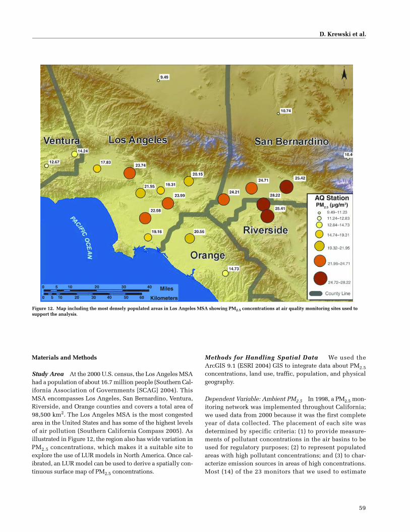
D. Krewski et al.
59
Materials and Methods
Study Area At the 2000 U.S. census, the Los Angeles MSAhad a population of about 16.7 million people (Southern Cal-ifornia Association of Governments [SCAG] 2004). ThisMSA encompasses Los Angeles, San Bernardino, Ventura,Riverside, and Orange counties and covers a total area of98,500 km2. The Los Angeles MSA is the most congestedarea in the United States and has some of the highest levelsof air pollution (Southern California Compass 2005). Asillustrated in Figure 12, the region also has wide variation inPM2.5 concentrations, which makes it a suitable site toexplore the use of LUR models in North America. Once cal-ibrated, an LUR model can be used to derive a spatially con-tinuous surface map of PM2.5 concentrations.
Methods for Handling Spatial Data We used theArcGIS 9.1 (ESRI 2004) GIS to integrate data about PM2.5concentrations, land use, traffic, population, and physicalgeography.
Dependent Variable: Ambient PM2.5 In 1998, a PM2.5 mon-itoring network was implemented throughout California;we used data from 2000 because it was the first completeyear of data collected. The placement of each site wasdetermined by specific criteria: (1) to provide measure-ments of pollutant concentrations in the air basins to beused for regulatory purposes; (2) to represent populatedareas with high pollutant concentrations; and (3) to char-acterize emission sources in areas of high concentrations.Most (14) of the 23 monitors that we used to estimate
Figure 12. Map including the most densely populated areas in Los Angeles MSA showing PM2.5 concentrations at air quality monitoring sites used to support the analysis.
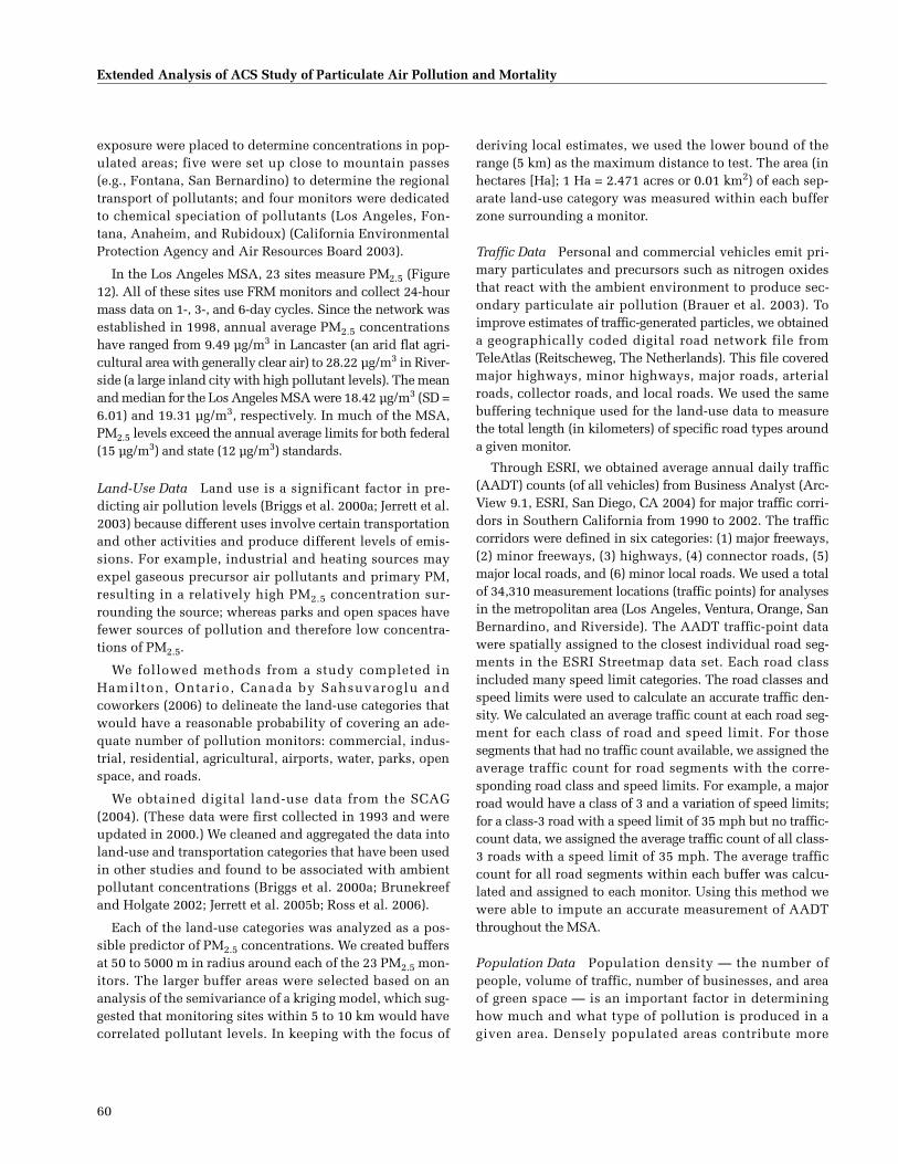
60
Extended Analysis of ACS Study of Particulate Air Pollution and Mortality
exposure were placed to determine concentrations in pop-ulated areas; five were set up close to mountain passes(e.g., Fontana, San Bernardino) to determine the regionaltransport of pollutants; and four monitors were dedicatedto chemical speciation of pollutants (Los Angeles, Fon-tana, Anaheim, and Rubidoux) (California EnvironmentalProtection Agency and Air Resources Board 2003).
In the Los Angeles MSA, 23 sites measure PM2.5 (Figure12). All of these sites use FRM monitors and collect 24-hourmass data on 1-, 3-, and 6-day cycles. Since the network wasestablished in 1998, annual average PM2.5 concentrationshave ranged from 9.49 µg/m3 in Lancaster (an arid flat agri-cultural area with generally clear air) to 28.22 µg/m3 in River-side (a large inland city with high pollutant levels). The meanand median for the Los Angeles MSA were 18.42 µg/m3 (SD =6.01) and 19.31 µg/m3, respectively. In much of the MSA,PM2.5 levels exceed the annual average limits for both federal(15 µg/m3) and state (12 µg/m3) standards.
Land-Use Data Land use is a significant factor in pre-dicting air pollution levels (Briggs et al. 2000a; Jerrett et al.2003) because different uses involve certain transportationand other activities and produce different levels of emis-sions. For example, industrial and heating sources mayexpel gaseous precursor air pollutants and primary PM,resulting in a relatively high PM2.5 concentration sur-rounding the source; whereas parks and open spaces havefewer sources of pollution and therefore low concentra-tions of PM2.5.
We followed methods from a study completed inHamilton, Ontario, Canada by Sahsuvaroglu andcoworkers (2006) to delineate the land-use categories thatwould have a reasonable probability of covering an ade-quate number of pollution monitors: commercial, indus-trial, residential, agricultural, airports, water, parks, openspace, and roads.
We obtained digital land-use data from the SCAG(2004). (These data were first collected in 1993 and wereupdated in 2000.) We cleaned and aggregated the data intoland-use and transportation categories that have been usedin other studies and found to be associated with ambientpollutant concentrations (Briggs et al. 2000a; Brunekreefand Holgate 2002; Jerrett et al. 2005b; Ross et al. 2006).
Each of the land-use categories was analyzed as a pos-sible predictor of PM2.5 concentrations. We created buffersat 50 to 5000 m in radius around each of the 23 PM2.5 mon-itors. The larger buffer areas were selected based on ananalysis of the semivariance of a kriging model, which sug-gested that monitoring sites within 5 to 10 km would havecorrelated pollutant levels. In keeping with the focus of
deriving local estimates, we used the lower bound of therange (5 km) as the maximum distance to test. The area (inhectares [Ha]; 1 Ha = 2.471 acres or 0.01 km2) of each sep-arate land-use category was measured within each bufferzone surrounding a monitor.
Traffic Data Personal and commercial vehicles emit pri-mary particulates and precursors such as nitrogen oxidesthat react with the ambient environment to produce sec-ondary particulate air pollution (Brauer et al. 2003). Toimprove estimates of traffic-generated particles, we obtaineda geographically coded digital road network file fromTeleAtlas (Reitscheweg, The Netherlands). This file coveredmajor highways, minor highways, major roads, arterialroads, collector roads, and local roads. We used the samebuffering technique used for the land-use data to measurethe total length (in kilometers) of specific road types arounda given monitor.
Through ESRI, we obtained average annual daily traffic(AADT) counts (of all vehicles) from Business Analyst (Arc-View 9.1, ESRI, San Diego, CA 2004) for major traffic corri-dors in Southern California from 1990 to 2002. The trafficcorridors were defined in six categories: (1) major freeways,(2) minor freeways, (3) highways, (4) connector roads, (5)major local roads, and (6) minor local roads. We used a totalof 34,310 measurement locations (traffic points) for analysesin the metropolitan area (Los Angeles, Ventura, Orange, SanBernardino, and Riverside). The AADT traffic-point datawere spatially assigned to the closest individual road seg-ments in the ESRI Streetmap data set. Each road classincluded many speed limit categories. The road classes andspeed limits were used to calculate an accurate traffic den-sity. We calculated an average traffic count at each road seg-ment for each class of road and speed limit. For thosesegments that had no traffic count available, we assigned theaverage traffic count for road segments with the corre-sponding road class and speed limits. For example, a majorroad would have a class of 3 and a variation of speed limits;for a class-3 road with a speed limit of 35 mph but no traffic-count data, we assigned the average traffic count of all class-3 roads with a speed limit of 35 mph. The average trafficcount for all road segments within each buffer was calcu-lated and assigned to each monitor. Using this method wewere able to impute an accurate measurement of AADTthroughout the MSA.
Population Data Population density — the number ofpeople, volume of traffic, number of businesses, and areaof green space — is an important factor in determininghow much and what type of pollution is produced in agiven area. Densely populated areas contribute more

D. Krewski et al.
61
traffic-related pollution than sparsely populated areas, andwithin a city density may also influence the content ofemissions (Ross et al. 2006). Higher population densitygenerates more pollution from heating buildings by com-bustion and from traffic for commuting and traveling tocommercial areas.
To determine the population density across the SCAGarea (the Los Angeles MSA plus Imperial County), we cal-culated a kernel estimate by assigning the U.S. Censuspopulation data for 2000 for each census tract to thecensus tract centroid. The radius of the kernel was deter-mined through analyses with a semivariogram. This pro-cess revealed that analyzing spatial autocorrelation in therange of 5 to 10 km would be optimal.
Physical Geography Proximity to a large body of water,such as an ocean, reduces the concentrations of pollutants,and the onshore marine breeze helps maintain pollution atlower levels near the coast (Bay Area Air Quality Manage-ment District [BAAQMD] 2005). The distance to thePacific ocean was calculated for each monitor location andwas analyzed for its possible relationship to measured pol-lutant levels in the LUR model. Elevation data wereacquired from the USGS at 30-m resolution and each mon-itoring area was assigned an elevation for analysis in theLUR model.
Modeling Methods Regression and spatial analysis wereused to create an interpolated PM2.5 pollutant surface. Arc-View v3.3, ArcMap v9.0, ArcInfo v9.0 (Redlands, CA), S-PLUS 2000 (Boston, MA) and Stata v8 (College Station, TX)were used for these analyses. We used an inverse distanceweighting (IDW) method to create an accurate surface.
Linear regression was conducted using the natural loga-rithm transformation of the PM2.5 measurements. Bivariatelinear regressions were first used to determine which vari-ables were most strongly related to PM2.5. This first steptested over 140 independent variables because land-useand road variables covered a large number of categoriesand several sizes of buffers around 23 monitors. A mul-tiple linear regression model was developed using the sig-nificant parameters from the bivariate linear regressionswith a manual forward selection process based on thehighest t test score for each variable. The VIF was thenexamined to identify variables that were collinear andcould be eliminated. Variables with the highest VIF andvariables with the lowest t scores were removed until aparsimonious model with the highest R2 value andacceptable levels of collinearity between included vari-ables was derived.
Using the bootstrap method, we completed a sensitivityanalysis to test the stability of the estimates from the mul-tiple regression model (Burrough and McDonnell 1998).From the 23 monitor data points, a random sample of 15data points was selected with replacement, for 1000 repe-titions. This enabled us to determine bias in the estimatesand how accurately the model would predict PM2.5 con-centrations when multiple locations (or monitors) wereexcluded from the regression analysis. Additional modeldiagnostics included the Cook-Weisberg test for heteroske-dasticity and the degrees of freedom Betas and Cook dis-tance to examine outliers.
Visualizing the Surface Visualization is an importantdiagnostic tool for assessing the face validity of a predictedLUR model. We used GIS software to identify approxi-mately 18,000 lattice points for the SCAG area with 2.3 kmbetween lattice points. We created lattice points that wererelatively close together in distance to more finely estimatethe PM2.5 surface, but we were partly constrained by com-putational capacity. Buffers for the land-use variables inthe final LUR model were created around each latticepoint, where the areas of each variable were once againcalculated in hectares. Using the fitted regression equa-tion, we calculated a predicted PM2.5 value for each of the18,000 lattice points. This method allowed us to visualizethe PM surface; for subsequent health analysis, geo-graphic points corresponding to study subjects couldserve as the lattice assignment points to minimize expo-sure assignment error.
We then used the IDW method to interpolate the pol-lutant surface. The IDW interpolator assumes that at eachPM2.5 sample point the local influence lessens with dis-tance (ESRI 2004). A specified number of predicted PM2.5points, or all points within a specified radius, can be usedto determine the output value for each location, creating asurface. The power in the IDW interpolation determineshow influential surrounding points are to the point beinginterpolated (Burrough and McDonnell 1998). A higherpower results in less influence from distant points (Bur-rough and McDonnell 1998). For this analysis we used thedefault power of 2, which is a common power used ininverse distance squared weighting.
Results
The land-use variables most correlated with PM2.5 con-centrations from monitors were used to develop the mul-tivariate model; correlation coefficients are shown inTable 21. The final LUR model included three indepen-dent variables (Table 22): (1) traffic count within 300 m(as a direct proxy for particulate emissions and gaseous

62
Extended Analysis of ACS Study of Particulate Air Pollution and Mortality
precursors), (2) industrial areas within 5000 m (to representprimary and precursor emissions), and (3) government areaswithin 5000 m (as a proxy for traffic intensity around majordestinations such as schools, government service offices,and hospitals). The R2 value for the LUR was 0.69 (F =14.07, P < 0.00001), with a few geographic areas near the
intersections of freeways displaying over-prediction (seeFigure 13).
Regression diagnostics were used to assess the validityof the LUR model. Table 22 shows little collinearityamong the independent variables; the average VIF was1.06. The visualization surface in Figure 14 shows a 63%R2 between the measured and predicted values of PM2.5from the LUR model. Although the residuals showed aslightly greater variance with higher PM2.5 concentrations(Figure 15), the Cook-Weisberg test for heteroskedasticityindicated a nonsignificant difference in the variancearound the residuals (P = 0.81), and the degrees-of-freedom Betas-and-Cook distance indicated few outliers inthe data. An additional sensitivity analysis used the boot-strap method, in which we resampled 15 locations with1000 repetitions and jackknife residual statistics. For thebootstrap, the bias values and standard errors wereextremely close to 0, and the statistics for the jackkniferesiduals were less than 0.01, indicating that no singlePM2.5 monitor’s data drove the values predicted.
Discussion
Accuracy of Predictions Using the LUR Model We deriveda multiple linear regression model that explained 69% ofthe variance in PM2.5 concentrations, with the main pre-dictors being traffic count within 300 m, industrial areaswithin 5000 m, and government areas within 5000 m(Table 22). In some areas, the LUR predicted PM2.5 concen-trations slightly higher than those measured — within theLos Angeles Basin near the intersection of high-traffic free-ways (605 and 210, 110 and 405, and 405 and 55) and inLong Beach near the two ports (Los Angeles and LongBeach) and the 710 freeway (Figures 13 and 14).
All of the observed over-predictions were located nearintersections of major freeways (Figure 13) and some wereupward of 126 µg/m3. Due to unregulated fuel combustion,ships are one of the leading sources of particulate air pol-lution in the Los Angeles Basin (Hricko 2004). Sur-rounding the ports is a network of freeways and railroad
Table 21. Land Use Variables with R � 0.4 That Were Significantly Associated with PM2.5 Concentrationsa
DescriptionBuffer Size
(m) R Value
Commercial areas 5000 0.67Industrial areas* 5000 0.58Parks and recreation 5000 0.55Population density 20 km 0.54
Collector roads 5000 0.53Arterial roads 3000 0.52Government areas* 5000 0.51Population density 10 km 0.48
Arterial roads 2000 0.48Traffic* 300 0.48Arterial roads 5000 0.47
Collector roads 2000 0.46Arterial roads 1000 0.45Collector roads 3000 0.45
Industrial areas 3000 0.42Arterial roads 750 0.4Minor roads 750 0.39
Commercial areas 750 0.35Industrial areas 50 0.32Open areas 2000 �0.43
Open areas 3000 �0.48Secondary roads 2000 �0.51Secondary roads 1000 �0.54Open areas 5000 �0.55
a Arranged from highest to lowest correlation. An * indicates the three variables used in the final model.
Table 22. Land-Use Regression Model Statistics Along with Collinearity Diagnostics
VariablesBuffer
(m) t Value SE P Value VIF
Constant 2.28621 22.81 0.1002109 0.000Traffic 300 0.00001 2.99 0.0000034 0.007 1.09Industrial area 5000 0.00032 3.33 0.0000958 0.004 1.05Government area 5000 0.00072 3.35 0.0002139 0.003 1.04
D. Krewski et al.
63
tracks used to disperse cargo to distribution and storagecenters in inland areas. More transport trucks, which com-bust diesel fuel, travel the 710 freeway than any otherfreeway in Los Angeles (Meyer 2003). Westerdahl and col-leagues (2005) found that measured freeway concentra-tions of PM2.5 had a range of 60 to 820 µg/m3 on the 10 Eastfreeway and that concentrations along major roadwayswith high-traffic density were up to 20 times higher thanresidential concentrations. Those measurements weretaken over a 5-day period in April of 2003, whereas ourLUR model estimates were based on data from 2000. More-over, in the Westerdahl study, increased concentrations ofPM2.5 were associated with high diesel traffic along free-ways. Thus, the over-predicted values in our analysis areat plausible levels, although further field validation workis needed to assess whether annual average levels on ornear freeway intersections are indeed this high.
Brauer and associates (2003) and Hochadel and col-leagues (2006) have also used LUR to predict PM2.5 con-centrations in Europe. Brauer’s team modeled air pollution
in communities throughout the Netherlands, in Munich,Germany, and in Stockholm, Sweden. Although they usedonly traffic indicators and did not use land-use classifica-tions in their multivariate regression model, they wereable to derive significant prediction models for each of thethree locations, for both PM2.5 mass and PM2.5 filter absor-bance, which is used as a marker for diesel exhaust (Braueret al. 2003). For the Netherlands, Munich, and Stockholm,the R2 values for the PM2.5 mass prediction model were0.78, 0.76, and 0.63, respectively; and 0.9, 0.83, and 0.76,respectively, for the PM2.5 absorbance prediction model.Since absorbance models are typically used to assesstraffic-related pollutants, the absorbance model results area better predictor of measured PM2.5 than the PM2.5 massmodel because the variables used in the absorbance modelwere chosen specifically to measure traffic. Hochadel andcoworkers (2006) conducted a study in Wesel, Germany,using primarily traffic-based indicators as the geographicfactors. The regression models predicted strongly for PM2.5
absorbance (R2 = 0.65), but not for PM2.5 mass (R2 = 0.094).
Figure 13. Map of over-predicted values from the LUR model, shown as > 50, 75, or 100 µg/m3 higher than the measured value. Most over-predictionsoccurred at freeway intersections. PM2.5 monitor positions are marked with a +.

64
Extended Analysis of ACS Study of Particulate Air Pollution and Mortality
Effects of Buffer Size Selection The buffers we used tomeasure areas of land-use categories were quite large com-pared with other studies (generally 100 to 300 meters;Brauer et al. 2003; Hochadel et al. 2006; Ross et al. 2006;Sahsuvaroglu et al. 2006). The Los Angeles MSA is a mas-sive and sprawling urban area and has one of the highestlevels of employment and population dispersion in theUnited States (Gordon and Richardson 1996). This dis-persed urban structure, transected by major highways andcommercial areas, leads to a broader regional scale ofinfluence for processes that generate PM pollution, and the2000- to 5000-m buffers surrounding the PM2.5 monitorsprobably reflect this dispersed form of urban development.
The study that is most closely related geographically tothis Los Angeles Analysis was done by Ross and associates(2006) in San Diego County, California, in which they pre-dicted ambient NO2 concentrations. The study area in San
Figure 14. PM2.5 surface created by IDW using predicted PM2.5 concentrations from an LUR model with the variables of traffic within a 300-m radius,industrial areas within a 5000-m radius, and government areas within a 5000-m radius. PM2.5 monitor positions are marked with a +. Notice the highPM2.5 concentrations near intersections of major highways.
Figure 15. Graph showing predicted PM2.5 versus measured PM2.5 con-centrations from the LUR model. The measured and predicted values foreach monitor are plotted on the x and y axes.

D. Krewski et al.
65
Diego County was much smaller than the Los AngelesMSA — 11,721 km2 versus 98,500 km2 for the SCAGregion. The traffic-count variable and the industrial land-use variable were common to both models, but the Rossstudy found that smaller-radius buffers were more effec-tive predictors than those we used in Los Angeles. Thismakes sense because NO2 arises from local sources and isknown to vary over smaller areas in proximity to traffic(Gilliland et al. 2005), whereas PM2.5 is a mixture gener-ated by primary and secondary sources that we wouldexpect to be more regionally dispersed. Data from the largerbuffer sizes in this study may reflect either an inherent spa-tial scale of variation in the pollutants or the more dispersedurban structure of Los Angeles.
Modeling Spatial Variability in Exposure A krigingmodel was previously developed for the Los Angeles Basinbased on PM2.5 values from the same 23 monitors (Jerrett etal. 2005). That model did not show as much of the local-areavariations in exposure as did the LUR model developed forthis study (see Figures 14 and 16). The success of this LURmodel demonstrates that traffic and land uses are strongpredictors of PM2.5 concentrations. Although the scale ofvariation of PM2.5 values around an emissions sourceappears to be larger than what we might expect from purelylocal processes, the covariance of PM2.5 concentrations
with land-use predictors suggests that local land uses andtraffic have a significant role in distributions of PM2.5
across this large urban area. The kriging model may not begeneralizable, because the monitors were established bygovernment agencies in certain locations for the purposeof regulatory compliance and therefore may not reflect thetrue variability in PM2.5 levels represented by the mixtureof land uses in the LUR model.
If the monitoring network is not representative of thespatial variability in actual pollutant exposures, we wouldexpect to see bias in the pollutant levels predicted frommodels based on those monitoring locations. Our use ofthe bootstrap method demonstrated that it is unlikely thatsingle influential points drove the results of the LURmodel. For example, none of the monitors were specifi-cally located to measure traffic impact, and the closestproxy we have is monitors located in densely populatedurban areas. Although there is some overlap betweendense population and areas of heavy traffic, we would beable to create kriging models to reflect greater local varia-tion if we could include data from monitors located nearheavy-traffic sites.
Although the spatially modeled exposures dependintrinsically on land use and local emissions sources suchas traffic, the fact that some covariates are related to factors
Figure 16. Universal kriging map of PM2.5 in the Los Angeles area. PM2.5 monitor positions are marked with a circled dot (�). (Adapted from Kuenzli etal. [2005].)

66
Extended Analysis of ACS Study of Particulate Air Pollution and Mortality
that affect health and mortality (such as socio-economicposition) means that the LUR model may include somehidden confounders. Consequently, to use LUR for pollu-tion and health analyses, researchers must adjust for othercontextual confounders that may be related to the land-useand traffic input to ensure unbiased estimates of the healtheffects of air pollution.
We found that LUR predicted 69% of the variance inPM2.5 mass in the Los Angeles MSA. With sensitivity anal-ysis, we observed that few monitors influenced the results.Traffic, industrial, and government areas were of most sig-nificance because of their associated particulate emissionsfrom increased traffic and industrial point sources. Furtherinvestigation is needed into the extraordinarily high levelsof PM2.5 predicted around the intersections of freeways;these levels may constitute a significant threat to publichealth if they are validated by monitoring.
SPATIAL ANALYSIS OF AIR POLLUTION AND MORTALITY IN LOS ANGELES
Materials and Methods
Study Population Mortality data were extracted from theACS CPS-II cohort database for metropolitan Los Angeles atthe ZCA scale (average population per ZCA in Los Angelesis approximately 35,000; average area is approximately22.5 km2). ZCA centroids were weighted by populationdistribution using spatial boundary files based on 1980and 1990 USBC data. The centroids were used to assignPM2.5 and O3 exposure levels to the 22,905 ACS subjectsliving in the 267 ZCAs (this cohort included 5,856 deathsbased on follow-up from 1982 through 2000). Some sub-jects reported only PO Box addresses and were thereforeexcluded. As in earlier ACS analyses (Pope et al. 2000; Jer-rett et al. 2005), availability of air pollution data and otherrelevant information (e.g., ZCA-level data about ecologiccovariates) led to the subset of study subjects to be used inthe health effects assessment. Although the ACS cohort isnot representative of the general population, the cohortallows for internally valid comparisons within large sam-ples of the American population.
Assessment of PM2.5 Exposure An LUR prediction modelwas developed to predict PM2.5 from 23 monitoring loca-tions in the Los Angeles MSA using GIS to integrate datafrom land use, transportation, and physical geography (seeA Land-Use Regression Model for Predicting PM2.5 in theLos Angeles Region). The LUR method explained 69% ofthe variance in PM2.5 with three predictors around eachmonitoring site: (1) traffic count within 300 m, (2) indus-trial land area within 5000 m, and (3) government land
area within 5000 m. Model validation suggested that onlya few areas were over-predicted in the downtown sectionand near freeway interchanges. (See above for details ofthe LUR model’s derivation and validation [also describedin Moore et al. 2007]).
Assessment of O3 Exposure In earlier ACS studies thatused between-city comparisons, few associations havebeen found between O3 exposure and mortality (Pope et al.1995, 2002; Krewski et al. 2000a,b). Nevertheless, expo-sure to this pollutant is considered a health threat in theLos Angeles region, which has some of the highest levelsin the United States (Künzli et al. 2003). For O3, weobtained data at 42 sites in and around the Los AngelesBasin from the California Air Resources Board (ARB) data-base. We interpolated two surfaces using a universalkriging algorithm: one surface based on the average of thefour highest 8-hour concentrations during 2000 at eachmonitoring site, and another based on the expected peakdaily concentrations (EPDC). Expected daily peaks havebeen used as a statistical measure to assess the likelihoodof exceeding the 8-hour average California standard ateach site; expected peaks are based on data recorded ateach site on a specific date in the previous 3 years (1999–2001). Both 8-hour concentrations and daily peaks areused for federal and state designations of nonattainmentareas. They both capture extreme events, but the expecteddaily peak concentration provides more stability for esti-mating spatial patterns than the one-year measures basedon the four highest days. Few studies of long-term healtheffects have found significant association with O3 expo-sure, although acute effects of a small magnitude havebeen observed (Bell et al. 2004). Thus, it seems plausiblethat an O3 effect would be manifest in those areas mostlikely to experience exceedances.
Traffic Data To assess the impact of traffic, we definedbuffers at both 500 and 1000 meters of a freeway. EachZCA centroid within those buffers was assigned a value of1 and others were assigned 0. The resulting variables wereused as indictors of proximity to freeways in the healtheffects models. For each ZCA centroid within those bufferswe collected land-use and PM2.5 data from monitors. TheU.S. Census Feature Class Codes define freeways as havinglimited access, a numbered assignment (e.g., a major stateor U.S. route), and a speed limit higher than 50 miles perhour (USCB 2004). The distance from the ZCA centroid tothe freeway was used as a proxy for exposure to traffic-related pollution, which may exert effects independent ofand in addition to specific pollutants such as PM2.5 and O3
that vary over larger areas (Hoek et al. 2002).
D. Krewski et al.
67
Ecologic Covariates We assembled data from the 1980USCB for seven ecologic covariates for the ZCAs to controlfor contextual neighborhood covariates (see sidebar). Con-textual effects occur when individual differences in ahealth outcome are associated with the group of variablesthat represent the social, economic, and environmentalsettings where the individuals live, work, or spend time(e.g., poverty or unemployment in a neighborhood) (Curtisand Taket 1996; Macintyre and Ellaway 2000; Pickett andPearl 2001; Diez Roux 2002). These contextual effectsoften operate independently from (or interactively with)the individual-level covariates, such as smoking and diet,from the ACS enrollment questionnaire. We used the eco-logic covariates that have been identified as important inthe population health literature and have been previouslytested as potential confounders with the ACS dataset at themetropolitan scale (Evans and Kantrowitz 2002; Willis etal. 2003). These included income, income disparity, grade12 education, total population, racial composition (black,white, Hispanic in percentages), and unemployment (Jer-rett et al. 2003).
We used the proportion of homes that have air condi-tioning to measure possible exposure misclassification onthe premise that air-conditioned houses are more tightlysealed and have lower penetration of particles from out-doors. Similar housing variables have been used in a meta-analysis of acute effects (Levy et al. 2000); and a recentstudy of personal exposures in Los Angeles reported thatparticle penetration is largely reduced in air-conditionedhomes (Meng et al. 2005). This variable added partial con-trol for the impact of air conditioning, which may relateboth to health outcomes (through prevention of heat stress)and to air pollutant concentrations (because high concen-trations and low proportions of air conditioning are relatedin our study area). We thus expected the proportion of airconditioning in the ZCA to correlate with lower PM expo-sures and effects.
We also computed principal components from the sevenecologic covariates (excluding AC) to provide maximalcontrol for confounding while avoiding multicollinearityamong the ecologic covariates (Luginaah et al. 2001;Krieger et al. 2002).
Statistical Methods and Data Analysis
The statistical methods are similar to those employed byJerrett and colleagues (2005a) in a previous intra-urbananalysis of data from Los Angeles using spatial kriging toestimate air pollutant concentrations at the ZCA scale.(The underlying statistical model is the random effectsCox model described in the section Nationwide Analysis /
Statistical Methods and Data Analysis / The RandomEffects Cox Model.)
In brief, we used the 44 individual-level covariates (seesidebar) identified as possible confounders of the air pol-lution–mortality association in the Updated Analysis(Pope et al. 2002). These variables included lifestyle, diet,demographics, occupational, and educational factorsalong with 12 variables that measure aspects of smoking.Sensitivity analyses revealed that removing individualvariables had little influence on the estimated risk of pol-lution exposure; therefore, to promote comparability withresults from earlier studies, we report the results for ouranalyses that included this standard set of 44 individual-level variables. Eight ecologic covariates (discussed above)were also included.
We used the standard Cox model for our main analysesof association between air pollution and mortality(Hosmer and Lemeshow 1999). Because the units of anal-yses were small ZCAs and previous analyses had indi-cated spatial autocorrelation in the residual variation ofsome health effects analyses, we also used the spatialrandom effects Cox model as a cross-validation of the stan-dard Cox model. We have previously shown that survivalexperience is clustered by community and the clusters arespatially autocorrelated between communities (Krewski etal. 2000a,b; Jerrett et al. 2003). Lack of statistical controlfor these factors can bias the estimates of the effects of airpollution and underestimate associated standard errors(Jerrett et al. 2003; Ma et al. 2003). We specified a model inwhich the random effects were assumed to be positivelycorrelated for neighboring ZCAs. Thiessen polygons,which ensure that all points within the polygon are closerto the centroid of that polygon than to any other centroid,were used to assign first-order nearest-neighbor contiguitybetween the ZCAs. The polygons were derived using Arc-View 3.2 (ESRI Corp., Redlands, CA).
Results
Using the new LUR model documented in the last sec-tion, we assigned exposure concentrations based on thetraffic, government, and industrial land use for the 267ZCAs (see also Jerrett et al. 2005a). These exposure assign-ments were then compared with the earlier analysis, withexactly the same causes of death, individual and ecologiccovariates, and copollutants. The results are shown inTable 23 (six causes of death are shown in each section ofthe table).
The results show the effects of LUR-predicted PM2.5exposure with different levels of control for confoundingvariables. HRs are expressed for a 10-µg/m3 change in

68
Extended Analysis of ACS Study of Particulate Air Pollution and Mortality
Tabl
e 23
.H
Rs
by C
ause
of D
eath
Ass
ocia
ted
wit
h E
ach
10-
µg/
m3 C
han
ge in
PM
2.5
2000
Con
cen
trat
ion
s (f
rom
LU
R M
odel
) Bas
ed o
n 2
67 L
os A
nge
les
ZC
Asa
Cov
aria
tes
All
Cau
ses
(n =
585
6)
IHD
ICD
-9: 4
10–4
14(n
= 1
462)
CP
DIC
D-9
: 400
–440
, 46
0–51
9(n
= 3
136)
Lu
ng
Can
cer
ICD
-9: 1
62(n
= 4
34)
Dig
esti
veC
ance
r(n
= 4
29)
Oth
erC
ance
rs(n
= 9
92)
PM
2.5
only
1.19
7 (1
.082
–1.3
25)
1.41
5 (1
.154
–1.7
35)
1.17
9 (1
.025
–1.3
56)
1.46
0 (1
.013
–2.1
05)
1.27
7 (0
.880
–1.8
54)
1.03
6 (0
.814
–1.3
19)
+ 4
4 In
div
idu
al-l
evel
cov
aria
tes
1.14
3 (1
.033
–1.2
66)
1.33
1 (1
.084
–1.6
34)
1.11
4 (0
.968
–1.2
82)
1.39
2 (0
.964
–2.0
10)
1.19
1 (0
.816
–1.7
38)
1.01
0 (0
.791
–1.2
89)
Eco
logi
c co
vari
ates
b
Air
con
dit
ion
ing
(%)
1.14
2 (1
.031
–1.2
65)
1.33
3 (1
.085
–1.6
38)
1.12
1 (0
.974
–1.2
90)
1.37
6 (0
.952
–1.9
89)
1.16
5 (0
.797
–1.7
02)
1.00
2 (0
.784
–1.2
81)
Bla
ck (
%)
1.14
5 (1
.033
–1.2
69)
1.34
7 (1
.096
–1.6
56)
1.12
0 (0
.972
–1.2
89)
1.41
1 (0
.976
–2.0
41)
1.18
8 (0
.812
–1.7
38)
1.00
9 (0
.789
–1.2
90)
Wh
ite
(%)
1.15
1 (1
.036
–1.2
78)
1.36
2 (1
.103
–1.6
82)
1.12
7 (0
.976
–1.3
02)
1.47
1 (1
.008
–2.1
47)
1.16
2 (0
.787
–1.7
17)
1.02
7 (0
.798
–1.3
21)
His
pan
ic (
%)
1.13
2 (1
.016
–1.2
61)
1.32
2 (1
.065
–1.6
41)
1.11
3 (0
.960
–1.2
90)
1.41
5 (0
.956
–2.0
96)
1.11
7 (0
.749
–1.6
67)
1.02
1 (0
.788
–1.3
23)
Un
emp
loym
ent
(%)
1.12
7 (1
.015
–1.2
52)
1.32
8 (1
.075
–1.6
41)
1.12
9 (0
.977
–1.3
05)
1.27
9 (0
.879
–1.8
62)
1.18
7 (0
.803
–1.7
55)
0.96
6 (0
.751
–1.2
43)
Med
ian
hou
seh
old
in
com
e ($
000s
)1.
146
(1.0
35–1
.268
)1.
332
(1.0
86–1
.635
)1.
115
(0.9
70–1
.283
)1.
388
(0.9
63–2
.001
)1.
195
(0.8
23–1
.735
)1.
014
(0.7
96–1
.293
)
Tota
l p
opu
lati
on1.
141
(1.0
30–1
.264
)1.
322
(1.0
76–1
.624
)1.
108
(0.9
63–1
.275
)1.
396
(0.9
67–2
.016
)1.
202
(0.8
23–1
.755
)1.
012
(0.7
92–1
.292
)
Inco
me
dis
par
ity
(Gin
i)1.
110
(0.9
99–1
.234
)1.
254
(1.0
14–1
.552
)1.
056
(0.9
13–1
.222
)1.
306
(0.8
93–1
.910
)1.
213
(0.8
23–1
.786
)1.
015
(0.7
90–1
.304
)
Gra
de
12 e
du
cati
on (
%)
1.14
4 (1
.033
–1.2
66)
1.33
4 (1
.087
–1.6
37)
1.11
8 (0
.972
–1.2
86)
1.38
6 (0
.961
–2.0
00)
1.18
3 (0
.811
–1.7
25)
1.00
6 (0
.788
–1.2
84)
Cov
aria
te g
rou
pin
gsA
ll s
ocia
l fa
ctor
s 1.
142
(1.0
26–1
.272
)1.
322
(1.0
64–1
.642
)1.
107
(0.9
54–1
.285
)1.
399
(0.9
49–2
.061
)1.
185
(0.8
00–1
.755
)1.
037
(0.8
03–1
.340
)
Air
con
dit
ion
ing,
med
ian
hou
seh
old
in
com
e, >
gra
de
12 e
du
cati
on, s
ocia
l fa
ctor
1.11
5 (1
.003
–1.2
39)
1.26
3 (1
.020
–1.5
63)
1.07
2 (0
.926
–1.2
41)
1.29
0 (0
.881
–1.8
90)
1.18
9 (0
.809
–1.7
48)
1.01
1 (0
.786
–1.2
99)
Par
sim
onio
us
ecol
ogic
cov
aria
tesc
1.12
6 (1
.014
–1.2
51)
1.26
4 (1
.022
–1.5
63)
1.08
6 (0
.939
–1.2
56)
1.31
1 (0
.897
–1.9
15)
1.19
9 (0
.817
–1.7
58)
1.01
2 (0
.788
–1.2
99)
Cop
ollu
tan
t co
ntr
old
44 I
nd
ivid
ual
-lev
el c
ovar
iate
s +
ozo
ne
(EP
DC
e )1.
191
(1.0
69–1
.327
)1.
455
(1.1
71–1
.810
)1.
187
(1.0
23–1
.378
)1.
446
(0.9
82–2
.128
)1.
163
(0.7
77–1
.742
)1.
059
(0.8
18–1
.371
)
44 I
nd
ivid
ual
-lev
el c
ovar
iate
s +
ozo
ne
(ave
rage
f )1.
176
(1.0
57–1
.307
)1.
431
(1.1
55–1
.772
)1.
152
(0.9
96–1
.334
)1.
489
(1.0
18–2
.178
)1.
166
(0.7
84–1
.734
)1.
053
(0.8
16–1
.358
)
44 I
nd
ivid
ual
-lev
el c
ovar
iate
s +
fre
eway
s w
ith
in 5
00 m
g1.
170
(1.0
54–1
.299
)1.
393
(1.1
27–1
.721
)1.
134
(0.9
82–1
.310
)1.
439
(0.9
89–2
.095
)1.
208
(0.8
19–1
.783
)1.
057
(0.8
24–1
.356
)
Cop
ollu
tan
t ri
sk e
stim
ates
Ozo
ne
(EP
DC
e )0.
985
(0.9
64–1
.006
)0.
973
(0.9
32–1
.015
)0.
966
(0.9
38–0
.994
)0.
989
(0.9
17–1
.068
)1.
008
(0.9
33–1
.089
)0.
989
(0.9
41–1
.040
)
Ozo
ne
(ave
rage
f )0.
993
(0.9
77–1
.010
)0.
984
(0.9
52–1
.017
)0.
985
(0.9
63–1
.008
)0.
970
(0.9
12–1
.032
)1.
007
(0.9
47–1
.070
)0.
993
(0.9
54–1
.033
)
Fre
eway
wit
hin
500
mg
0.98
7 (0
.875
–1.1
13)
0.89
8 (0
.706
–1.1
43)
0.91
5 (0
.775
–1.0
81)
1.44
0 (0
.939
–2.2
08)
0.84
1 (0
.526
–1.3
46)
1.18
4 (0
.883
–1.5
88)
Fre
eway
wit
hin
100
0 m
g0.
974
(0.8
94–1
.062
)1.
048
(0.8
85–1
.241
)0.
982
(0.8
74–1
.104
)0.
942
(0.6
85–1
.295
)0.
879
(0.6
34–1
.220
)0.
897
(0.7
21–1
.117
)
Tabl
e co
nti
nu
es n
ext
pag
e
a Bas
elin
e H
Rs
wer
e st
rati
fied
by
age
(in
1-y
ear
grou
pin
gs),
gen
der
, an
d r
ace.
Tot
al n
um
ber
of p
arti
cip
ants
was
22,
905.
HR
s ar
e fo
llow
ed b
y 95
% c
onfi
den
ce i
nte
rval
s. B
old
ed d
ata
refe
r to
tex
t.
b Eco
logi
c co
vari
ates
wer
e in
clu
ded
on
e at
a t
ime
in t
he
mod
el w
ith
PM
2.5
and
th
e 44
in
div
idu
al-l
evel
cov
aria
tes.
c
Par
sim
onio
us
ind
ivid
ual
-lev
el (2
3) a
nd
eco
logi
c (4
) cov
aria
tes
wer
e co
nsi
der
ed. T
he
ecol
ogic
cov
aria
tes
wer
e ai
r co
nd
itio
nin
g, h
ouse
hol
d in
com
e, g
rad
e 12
ed
uca
tion
, an
d th
e p
red
icte
d v
alu
es o
f th
e th
ird
pri
nci
pal
com
pon
ent
anal
ysis
bas
ed o
n a
ll s
ocia
l va
riab
les
(exc
ept
air
con
dit
ion
ing)
.d A
ll m
odel
s in
clu
ded
PM
2.5.
e B
ased
on
exp
ecte
d p
eak
dai
ly c
once
ntr
atio
ns.
f Ave
rage
of
fou
r h
igh
est
8-h
our
max
imu
m r
ead
ings
. g I
nte
rsec
tion
wit
h a
fre
eway
wit
hin
500
or
1000
m o
f a
ZC
A c
entr
oid
.
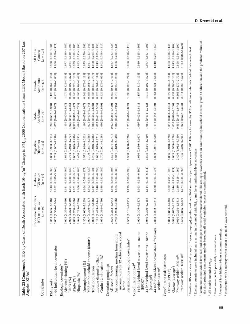
D. Krewski et al.
69
Tabl
e 23
(Con
tin
ued
).H
Rs
by C
ause
of D
eath
Ass
ocia
ted
wit
h E
ach
10-
µg/
m3 C
han
ge in
PM
2.5
2000
Con
cen
trat
ion
s (f
rom
LU
R M
odel
) Bas
ed o
n 2
67 L
os
An
gele
s Z
CA
sa
Cov
aria
tes
En
doc
rin
e D
isor
der
sIC
D-9
: 240
–279
(n =
95)
Dia
bete
sIC
D-9
: 250
(n =
57)
Dig
esti
veD
isor
der
s(n
= 1
51)
Mal
eA
ccid
ents
(n =
75)
Fem
ale
Acc
iden
ts(n
= 4
7)
All
Oth
erC
ause
s(n
= 4
97)
PM
2.5
only
3.34
4 (1
.565
–7.1
48)
2.31
3 (0
.803
–6.6
60)
1.86
8 (0
.993
–3.5
14)
1.22
6 (0
.512
–2.9
38)
1.12
6 (0
.367
–3.4
56)
0.97
8 (0
.692
–1.3
81)
+ 4
4 In
div
idu
al-l
evel
cov
aria
tes
3.03
7 (1
.384
–6.6
64)
2.02
2 (0
.687
–5.9
48)
1.70
9 (0
.902
–3.2
38)
1.07
8 (0
.443
–2.6
27)
0.92
8 (0
.284
–3.0
35)
1.00
6 (0
.709
–1.4
27)
Eco
logi
c co
vari
ates
b
Air
con
dit
ion
ing
(%)
3.02
5 (1
.374
–6.6
60)
2.02
1 (0
.685
–5.9
69)
1.68
3 (0
.885
–3.1
99)
1.15
6 (0
.470
–2.8
47)
1.07
0 (0
.322
–3.5
63)
0.97
7 (0
.688
–1.3
87)
Bla
ck (
%)
2.91
9 (1
.328
–6.4
19)
1.99
1 (0
.680
–5.8
30)
1.73
4 (0
.918
–3.2
77)
1.02
9 (0
.417
–2.5
35)
0.98
7 (0
.302
–3.2
22)
0.98
1 (0
.689
–1.3
96)
Wh
ite
(%)
2.81
5 (1
.256
–6.3
06)
1.97
1 (0
.657
–5.9
15)
1.68
2 (0
.875
–3.2
36)
0.97
3 (0
.387
–2.4
47)
0.94
3 (0
.279
–3.1
92)
0.97
9 (0
.682
–1.4
05)
His
pan
ic (
%)
2.94
9 (1
.283
–6.7
80)
2.00
6 (0
.640
–6.2
86)
1.45
6 (0
.744
–2.8
53)
1.08
8 (0
.424
–2.7
93)
0.69
3 (0
.198
–2.4
25)
1.03
3 (0
.713
–1.4
96)
Un
emp
loym
ent
(%)
2.35
9 (1
.065
–5.2
25)
1.66
4 (0
.568
–4.8
77)
1.57
2 (0
.818
–3.0
22)
1.19
0 (0
.474
–2.9
87)
0.94
4 (0
.279
–3.1
93)
0.97
5 (0
.679
–1.3
99)
Med
ian
hou
seh
old
in
com
e ($
000s
)2.
907
(1.3
29–6
.357
)1.
992
(0.6
81–5
.829
)1.
709
(0.8
97–3
.256
)1.
075
(0.4
39–2
.734
)0.
885
(0.2
61–2
.999
)1.
021
(0.7
23–1
.441
)
Tota
l p
opu
lati
on3.
090
(1.4
01–6
.816
)2.
017
(0.6
86–5
.924
)1.
735
(0.9
16–3
.286
)1.
083
(0.4
45–2
.638
)0.
835
(0.2
49–2
.797
)1.
000
(0.7
04–1
.421
)
Inco
me
dis
par
ity
(Gin
i)3.
121
(1.4
23–6
.844
)2.
048
(0.6
92–6
.059
)1.
691
(0.8
75–3
.271
)1.
027
(0.4
11–2
.563
)0.
920
(0.2
67–3
.178
)1.
013
(0.7
05–1
.453
)
Gra
de
12 e
du
cati
on (
%)
3.05
8 (1
.384
–6.7
59)
2.03
8 (0
.682
–6.0
89)
1.70
5 (0
.901
–3.2
28)
1.09
6 (0
.449
–2.6
80)
0.92
3 (0
.279
–3.0
59)
1.00
2 (0
.708
–1.4
17)
Cov
aria
te g
rou
pin
gsA
ll s
ocia
l fa
ctor
s 2.
676
(1.2
13–5
.904
)1.
985
(0.6
69–5
.895
)1.
571
(0.8
04–3
.071
)0.
927
(0.3
55–2
.420
)0.
650
(0.1
75–2
.414
)1.
057
(0.7
33–1
.525
)
Air
con
dit
ion
ing,
med
ian
hou
seh
old
in
com
e, >
gra
de
12 e
du
cati
on, s
ocia
l fa
ctor
2.79
6 (1
.203
–6.4
96)
1.88
5 (0
.584
–6.0
80)
1.31
1 (0
.649
–2.6
49)
1.08
8 (0
.432
–2.7
45)
0.91
0 (0
.256
–3.2
30)
1.00
6 (0
.702
–1.4
41)
Par
sim
onio
us
ecol
ogic
cov
aria
tesc
2.55
9 (1
.131
–5.7
91)
1.73
5 (0
.569
–5.2
90)
1.33
0 (0
.660
–2.6
79)
1.21
0 (0
.488
–3.0
02)
1.09
6 (0
.320
–3.7
46)
0.98
8 (0
.690
–1.4
13)
Cop
ollu
tan
t co
ntr
old
44 I
nd
ivid
ual
-lev
el c
ovar
iate
s +
ozo
ne
(EP
DC
e )2.
926
(1.3
05–6
.557
)2.
063
(0.6
86–6
.200
)1.
630
(0.8
39–3
.167
)1.
097
(0.4
24–2
.841
)1.
157
(0.3
19–4
.195
)0.
939
(0.6
45–1
.368
)
44 I
nd
ivid
ual
-lev
el c
ovar
iate
s +
ozo
ne
(ave
rage
f )3.
040
(1.3
76–6
.715
)2.
154
(0.7
35–6
.311
)1.
575
(0.8
14–3
.049
)1.
060
(0.4
14–2
.712
)1.
014
(0.2
92–3
.525
)0.
967
(0.6
67–1
.401
)
44 In
div
idu
al-l
evel
cov
aria
tes
+ fr
eew
ays
wit
hin
500
mg
2.81
3 (1
.252
–6.3
21)
1.82
0 (0
.595
–5.5
74)
1.86
9 (0
.981
–3.5
60)
1.11
4 (0
.448
–2.7
69)
0.76
1 (0
.221
–2.6
18)
1.01
0 (0
.704
–1.4
50)
Cop
ollu
tan
t ri
sk e
stim
ates
Ozo
ne
(EP
DC
e )1.
044
(0.8
84–1
.232
)0.
982
(0.7
91–1
.220
)1.
036
(0.9
10–1
.179
)1.
015
(0.8
43–1
.224
)0.
872
(0.6
82–1
.114
)1.
063
(0.9
88–1
.144
)
Ozo
ne
(ave
rage
f )0.
999
(0.8
77–1
.137
)0.
944
(0.7
95–1
.121
)1.
063
(0.9
59–1
.178
)1.
037
(0.8
92–1
.206
)0.
931
(0.7
66–1
.132
)1.
043
(0.9
86–1
.104
)
Fre
eway
wit
hin
500
mg
0.66
0 (0
.264
–1.6
51)
0.43
9 (0
.116
–1.6
65)
2.49
0 (1
.082
–5.7
30)
0.55
9 (0
.167
–1.8
74)
0.86
8 (0
.279
–2.7
04)
0.86
8 (0
.584
–1.2
90)
Fre
eway
wit
hin
100
0 m
g1.
515
(0.8
55–2
.687
)1.
774
(0.8
35–3
.766
)0.
495
(0.2
46–0
.995
)1.
077
(0.5
27–2
.202
)2.
011
(0.8
83–4
.579
)1.
152
(0.8
68,1
.529
)
a B
asel
ine
HR
s w
ere
stra
tifi
ed b
y ag
e (i
n 1
-yea
r gr
oup
ings
), g
end
er, a
nd
rac
e. T
otal
nu
mbe
r of
par
tici
pan
ts w
as 2
2,90
5. H
Rs
are
foll
owed
by
95%
con
fid
ence
in
terv
als.
Bol
ded
dat
a re
fer
to t
ext.
b E
colo
gic
cova
riat
es w
ere
incl
ud
ed o
ne
at a
tim
e in
th
e m
odel
wit
h P
M2.
5 an
d t
he
44 i
nd
ivid
ual
-lev
el c
ovar
iate
s.
c P
arsi
mon
iou
s in
div
idu
al-l
evel
(23)
an
d e
colo
gic
(4)
cova
riat
es w
ere
con
sid
ered
. Th
e ec
olog
ic c
ovar
iate
s w
ere
air
con
dit
ion
ing,
hou
seh
old
in
com
e, g
rad
e 12
ed
uca
tion
, an
d th
e p
red
icte
d v
alu
es o
f th
e th
ird
pri
nci
pal
com
pon
ent
anal
ysis
bas
ed o
n a
ll s
ocia
l va
riab
les
(exc
ept
air
con
dit
ion
ing)
.d A
ll m
odel
s in
clu
ded
PM
2.5.
e B
ased
on
exp
ecte
d p
eak
dai
ly c
once
ntr
atio
ns.
f Ave
rage
of
fou
r h
igh
est
8-h
our
max
imu
m r
ead
ings
. g
Inte
rsec
tion
wit
h a
fre
eway
wit
hin
500
or
1000
m o
f a
ZC
A c
entr
oid
.

70
Extended Analysis of ACS Study of Particulate Air Pollution and Mortality
PM2.5 exposure (followed by the 95% CI). For example, wefollow the successive analyses for all-cause mortality:
• with PM2.5 alone (stratified for age, sex, and race), the HR was 1.197 (95% CI, 1.082–1.325);
• whereas with the 44 individual-level covariates the HR was 1.143 (95% CI, 1.033–1.266).
• All subsequent results include the 44 individual-level covariates and one or more ecologic covariates.
• With the 44 individual-level covariates and the eco-logic covariate of unemployment, the HR of PM2.5 was 1.127 (95% CI, 1.015–1.252).
• When we added four social factors extracted from the principal component analysis (which account for 81% of the total variance in the social variables), the HR was 1.142 (95% CI, 1.026–1.272).
• Including all ecologic covariates that were individu-ally associated with mortality in bivariate models with PM2.5 exposure (air conditioning, median income, and education attainment) reduced the HR to 1.115 (95% CI, 1.003–1.239).
• For the parsimonious model that included ecologic confounder variables that both reduced the pollution coefficient and had associations with mortality, the HR was 1.126 (95% CI, 1.014–1.251).
• When controlled for the expected peak daily O3 levels the HR was 1.191 (95% CI, 1.069–1.327). (Thus, simi-lar to earlier results [Jerrett et al. 2005], O3 had no pri-mary effect in these models for all-cause mortality.)
Discussion and Conclusions
In general, the associations for PM2.5 and mortality inthis set of analyses are similar in magnitude with thosereported earlier from geostatistical kriging estimates (Jer-rett et al. 2005a) with three minor differences. First, the HRfor PM2.5 alone is somewhat smaller than the risks fromthe kriging model. Second, although the risk estimateswere smaller in this study, the CIs were tighter. Third, theresults from this study appear to be less sensitive to eco-logic confounding. For example, in the earlier study, theparsimonious model for all-cause mortality that includedall the individual-level variables and the significant eco-logic confounders resulted in the lower confidence boundbelow 1. In this analysis, the same model had a lower confi-dence bound higher than 1 (1.126, 95% CI, 1.014–1.251;only the income disparity variable confounded the estimateto below 1, but that estimate was still extremely close to 1;see Table 23). We consider the model containing the socialfactors from the principal components analysis to be themost reasonable on the grounds that it maximally controlsfor confounding without inducing as much collinearity.
The estimates from the model that contains only the 44individual-level covariates (1.143, 95% CI, 1.033–1.266)and the model with all social factors (1.142, 95% CI,1.026–1.272) produce nearly identical point estimates.The CIs are only slightly wider for the model with socialfactors from the principal component analysis incorpo-rated in the model in the same manner as the ecologic fac-tors. Thus, results from this LUR exposure model appear tobe more robust to adjustment for confounders than the ear-lier results using the kriging surface.
The Los Angeles Analysis was extended using therandom effects Cox model with and without allowance forspatial autocorrelation. The earlier study (Jerrett et al.2005a) using the kriging estimates demonstrated signifi-cant autocorrelation in the risks, which was diminished toacceptable levels when the ecologic covariates wereincluded in the model. That analysis did not explicitlyincorporate a spatial autocorrelation parameter in themodel, but in the current analysis we used the full randomeffects formulation.
Table 24 displays results from the random effectsmodels, organized to compare results between modelswith and without allowance for spatial autocorrelation. Italso compares models with various levels of control forconfounding, beginning with a model that contains onlythe 44 individual-level covariates and no pollutant vari-able (all models were stratified for age, sex, and race). Theinitial model (with only the 44 individual-level covariates)thus demonstrates the residual random effects varianceattributable to variability in mortality patterns betweenZCAs. For all-cause mortality, when PM2.5 was included inthe model, random effects variance declined about 37%for the model with no autocorrelation (7.008 vs. 4.386) andabout 24% for the model including autocorrelation (10.02vs. 7.591). This large decline suggests that approximatelyone-third to one-quarter of the residual variation isaccounted for by the PM2.5 variable. The drop in therandom effects variance for models including ecologiccovariates was much larger, which indicates that thesevariables account for much of the residual variation inmortality across Los Angeles. Including the freeway inter-section variable (distance from a ZCA centroid to afreeway) yielded only a minimal change in the randomeffects variance. Substantial autocorrelation was stillfound in the data after inclusion of all the variables, as evi-denced by the fact that our estimate of ZCA autocorrela-tion reached the maximum value allowable in the modelformulation.
This high level of residual autocorrelation, even with avery small random effects variance, may have resultedfrom a number of phenomena. First, the nearest-neighbor

D. Krewski et al.
71
formulation of the random effects Cox model may not cap-ture what is likely to be a more complex residual spatialstructure. Second, the autocorrelation may not be sta-tionary over the entire study area, and more flexiblemodels based on spatial moving averages may be neededto capture this nonstationarity. Third, the presence of spa-tial autocorrelation may also suggest that one or moreimportant covariates have been excluded from the model.We have visually examined the residuals, and there seemsto be a clustering of autocorrelation in residual mortalityon the downwind side of roadways with high volumes oftruck traffic. The assignment of residence locations to theZCA centroid prevented us from precisely assigning expo-sures, but this autocorrelation suggests that possible effectsfrom truck traffic merit attention in future studies. Althoughthese theoretical possibilities are present, the point esti-mates and CIs are insensitive to model specification.
In analyses of IHD mortality, including PM2.5 had amarked effect on the residual random effects variance,with a drop of more than 86% (4.357 vs. 0.582). The subse-quent decline in the random effects variance due to inclu-sion of the ecologic covariates was also large, but muchless pronounced than with all-cause mortality. For IHD,
the residual autocorrelation was negligible. We expectedthis in a model in which the individual, ecologic, and airpollution variables predicted the mortality data more com-pletely than they did for the analysis of all-cause mortality.With IHD we did observe some confounding effect of thepoint estimates when we included the ecologic andfreeway variables. Models with and without the autocorre-lation parameter produced nearly identical results, aswould be expected with such a small amount of residualautocorrelation.
Results from the more refined exposure surface from theLUR model largely confirm the earlier findings from thekriging models. This is somewhat surprising given the dif-ferent visual appearance of each surface, with the LURdetecting smaller variations in areas around highways andindustry. The effect sizes were slightly diminished com-pared with the earlier study, but the effects shown in thisstudy tended to be less sensitive to control for con-founding and to alternative model specification. The largerdecline in the random effects variance for IHD mortalitysupports a growing body of research on the mechanisms ofsystemic pulmonary inflammation and atherogenesis(Brook et al. 2004; Künzli et al. 2005).
Table 24. Sensitivity Analysis Using the Random Effects Cox Model for a 10-µg/m3 Change in PM2.5 Exposure with Allowance for Spatial Autocorrelationa
Covariatesb
No Spatial Autocorrelation
Spatial Autocorrelation
HR
ZCAVariance (� 10�3) HR
ZCA Variance (� 10�3)
ZCAAuto-
correlation
All Causes44 Individual-level covariates — 7.008 — 10.02 0.3307c
+ PM2.5 1.158 (1.035–1.295) 4.386 1.160 (1.021–1.317) 7.591 0.3307c
+ Parsimonious ecologic covariatesd 1.152 (1.034–1.283) 0.229 1.152 (1.032–1.286) 0.623 0.3307c
+ Freeway intersectione 1.156 (1.036–1.289) 0.233 1.156 (1.034–1.293) 0.847 0.3307c
IHD44 Individual-level covariates — 4.357 — 4.357 0.000f
+ PM2.5 1.402 (1.137–1.728) 0.582 1.402 (1.137–1.728) 0.582 0.000f
+ Parsimonious ecologic covariatesd 1.347 (1.083–1.675) 0.189 1.347 (1.083–1.675) 0.189 0.000f
+ Freeway intersectione 1.339 (1.074–1.669) 0.189 1.339 (1.074–1.669) 0.189 0.000f
a Bolded data refer to text.b Covariates accumulate in the model with each addition.c Estimate of ZCA autocorrelation reached its maximum value.d Parsimonious individual-level (23) and ecologic (4) covariates were considered. The ecologic covariates were air conditioning, household income, grade
12 education, and the predicted values of the third principal component analysis based on all social variables (except air conditioning). e Intersection with a freeway within 500 or 1000 m of a ZCA centroid.f Estimate of ZCA autocorrelation was < 0.
72
Extended Analysis of ACS Study of Particulate Air Pollution and Mortality
CRITICAL EXPOSURE TIME WINDOWS
We constructed individual time-dependent exposureprofiles for particulate and gaseous air pollution for a sub-cohort of the ACS CPS-II in order to examine if there is acritical exposure time window that is primarily respon-sible for the increased mortality associated with ambientair pollution. We examined air pollution exposures inthree separate time windows: 1 to 5, 6 to 10, and 11 to 15years in the past.
MATERIALS AND METHODS
Study Population
The ACS CPS-II cohort consists of nearly 1.2 millionAmericans enrolled in 1982. In 1992 and 1993, the Nutri-tion Cohort was established within the larger ACS CPS-IIcohort (Calle et al. 2002). The purposes of selecting theNutrition Cohort were to update a variety of behavioral,medical, and demographic information that had first beencollected in 1982, and to collect more detailed dataregarding diet, physical activity, and other lifestyle factorsthat had not been obtained at the time of enrollment. TheACS cohorts and survey questionnaires are detailed else-where (Pope et al. 1995; Calle et al. 2002). Briefly, CPS-IIparticipants who were alive and between the ages of 50and 74 years and who resided in one of the following 21states that have population-based cancer registries wereincluded in the Nutrition Cohort: California, Connecticut,Florida, Georgia, Illinois, Iowa, Louisiana, Maryland, Mas-sachusetts, Michigan, Minnesota, Missouri, New Jersey,New Mexico, New York, North Carolina, Pennsylvania,Utah, Virginia, Washington, and Wisconsin. A total of184,194 participants from the CPS-II cohort who lived inthese states completed the self-administered questionnairemailed in 1992–1993, and were contacted again in 1997–1998, 1999–2000, and every 2 years thereafter for follow-up information. Mortality of the study participants wasascertained by volunteers in 1984, 1986, and 1988, andsubsequently by ACS staff using the National Death Index(Calle and Terrell 1993). The Emory University School ofMedicine Human Investigations Committee approved allaspects of the CPS II study.
Individual Exposure Profiles
Previous analyses of the ACS cohort have assumed thateach individual’s exposure was determined by the averagelevel of ambient air pollution in that person’s city of resi-dence at one point in time, either the beginning or the endof the study (Pope et al. 1995, 2002; Jerrett et al. 2005a;Krewski et al. 2000a,b). In this project, we sought to estab-
lish time-dependent exposure profiles for each individualin the study and to investigate the association betweenmortality and ambient air pollutant concentrations in spe-cific time windows that could reflect past exposures. Wehypothesized that a critical exposure time window may beprimarily responsible for the increased mortality associ-ated with ambient air pollution.
Individual time-dependent exposure profiles for PM2.5and SO2 were constructed for each participant bymatching the reported addresses at different times with theair pollutant exposure for the MSA where they lived. Indi-vidual exposures were determined using mean annualPM2.5 and SO2 levels that may have been experienced bythe individual during specific time windows. Forexample, to test the possibility that current excess mor-tality is primarily due to pollution exposure 5 to 10 yearsago, a person’s exposure would be modeled as the averageof his or her annual exposures during the intervalextending from 5 to 10 years before the current time.
Residential Histories Residential histories for the Nutri-tion Cohort participants were constructed based on theplace of residence when enrolled in the CPS-II study(1982), again when enrolled in the Nutrition Cohort (1992–1993), and at subsequent follow-up times in 1997–1998and 1999–2000. Zip Code information was used to assignparticipants to an MSA. Since no information was col-lected on the number of moves between follow-up stages,we assumed that if a new Zip Code was reported at thetime of follow-up, the participant had moved only oncedirectly from the previous Zip Code to the new one(Hansen 1998). Since no information on the time of a movewas collected between questionnaires, we randomlyassigned a year of move to each participant (Schachter2000) and assumed they had moved mid-calendar year(Hansen 1998). We constructed residential histories beforeenrollment in 1982 under the assumption that participantshad lived in the same residence they reported in 1982.
PM2.5 A total of 60,941 Nutrition Cohort participantsresided in one of 83 MSAs for which average annual PM2.5exposure data had been estimated based on measuredvalues of TSP and PM10 for the period of 1972–2000 (cal-culated by Lall and colleagues [2004]). For each MSA,either annual TSP or PM10 data were used in addition tothe specific PM2.5/TSP or PM2.5/PM10 ratio. This subco-hort was designated as the PM2.5-A group and PM2.5 expo-sure levels were assigned to each participant (Figure 17). Atotal of 8181 (13.4%) participants in the PM2.5-A groupmoved at least once during the study period. A small pro-portion of these participants (8.1%) did not reside in oneof the 83 MSAs for some portion of the follow-up period.

D. Krewski et al.
73
Figure 17. Profile of time trends (1972–2000) in average annual PM2.5 concentrations based on measured values of TSP and PM10 in 83 MSAs and onlinear interpolation of measured PM2.5 data for the years 1979–1983 and 1999–2000 for an additional 23 MSAs. (Figure continues next page.)
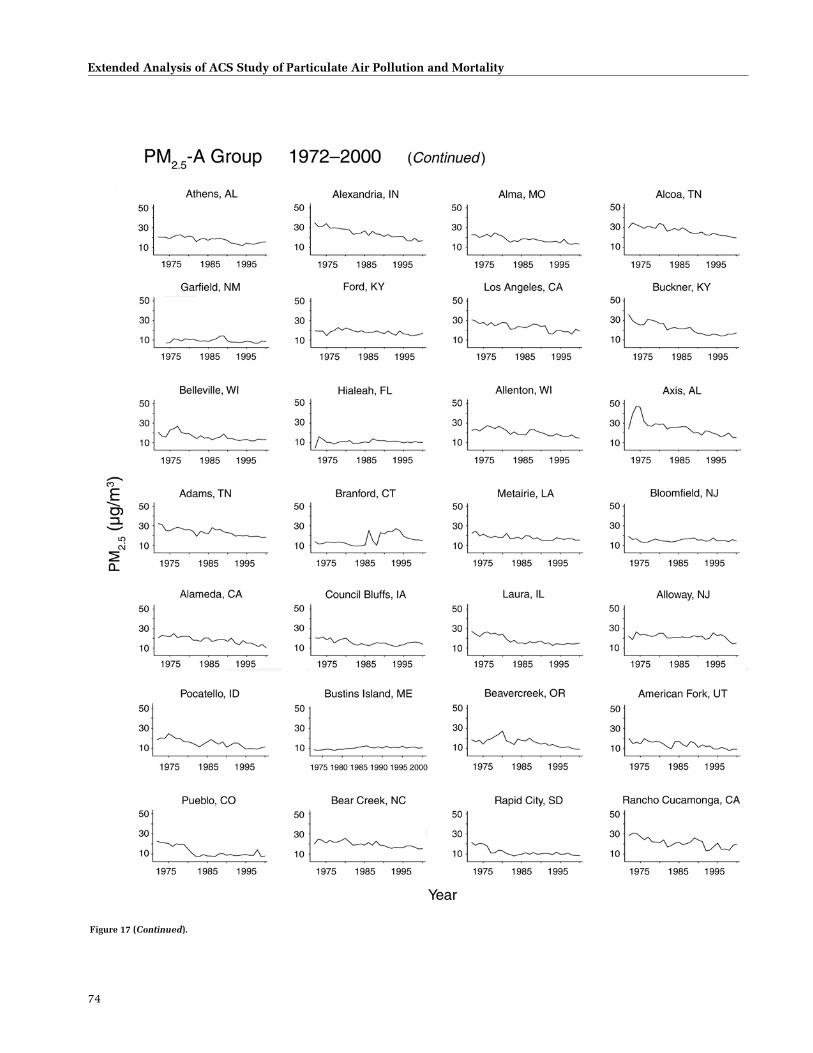
74
Extended Analysis of ACS Study of Particulate Air Pollution and Mortality
Figure 17 (Continued).
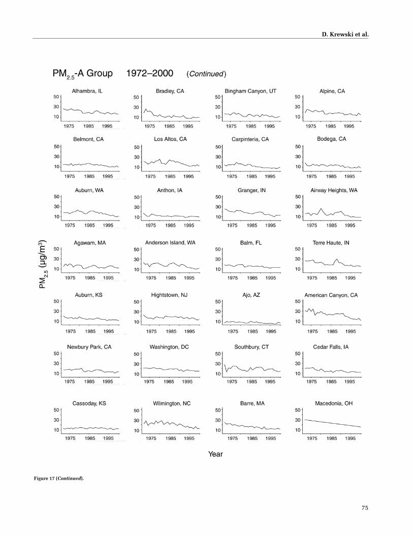
D. Krewski et al.
75
Figure 17 (Continued).

76
Extended Analysis of ACS Study of Particulate Air Pollution and Mortality
Figure 17 (Continued).

D. Krewski et al.
77
For those individuals, average annual PM2.5 concentra-tions were estimated using linear interpolation of datafrom an additional 23 MSAs for which measured PM2.5data were available for the periods 1979–1983 and 1999–2000 (Pope et al. 2002). The first participant in this groupdied in 1992; therefore, the entire exposure period weexamined for this group started in 1977 (15 years beforethe first death) and ended in 2000 (the end of follow-up).
A second analytic cohort was formed to include 81,466deceased participants from the full CPS-II cohort who (1)were not in the PM2.5-A group, and (2) died in the sameMSA where they had resided at enrollment in 1982. Theywere designated as the PM2.5-B group. We assumed thatthese participants had not moved between enrollment anddeath. PM2.5 values were assigned using average annualdata from Lall and colleagues (2004) for 50,915 participantsin 30 MSAs, and by linear interpolation of data for 23MSAs from Pope and colleagues (2002) for the remaining30,551 participants (Figure 18). The first participant in thisgroup died in 1982; therefore the exposure period rangedfrom 1967 (15 years before the first death) to 2000 (end offollow-up). The 1972 PM2.5 concentrations were used torepresent exposures before 1972. Participants in the PM2.5-A and PM2.5-B groups were mutually exclusive.
SO2 A third analytic group was formed with 80,711Nutrition Cohort participants who resided in one of 120MSAs for which at least 20 years of annual average SO2measurements were available. For most of the period from1972 to 2000, measured average annual SO2 data wereavailable from the EPA AIRS (Pope et al. 2002). Linearinterpolation between adjacent time points was used foryears in which average annual measurements weremissing (Figures 19 and 20). As with the PM2.5-A group,the entire exposure period examined was 1977 to 2000. Atotal of 5762 (7.1%) participants moved at least onceduring the exposure period.
STATISTICAL METHODS AND DATA ANALYSIS
Standard Cox models with time-dependent PM2.5 andSO2 exposure data were used to obtain adjusted HRs and95% CIs (SAS version 9.1; SAS Institute, Cary, NC) forall-cause, lung-cancer (ICD9: 162), and CPD (ICD9: 400–440, 460–519) mortality. For the PM2.5-A group and theSO2 group, HRs were calculated from enrollment in theNutrition Cohort in 1992–1993 through 2000. For thePM2.5-B group, the HRs covered the period from enroll-ment in the CPS-II full cohort in 1982 through end offollow-up in 2000.
The baseline hazard function was stratified by age (in 1-year groupings), sex, and race (white/other; from CPS-II
enrollment questionnaire). Models were adjusted for thestandard suite of 44 lifestyle and demographic variablescollected at enrollment in 1982 (see sidebar) including:smoking, education, marital status, body mass index,alcohol consumption, occupational exposure, and diet(Jerrett et al. 2005a; Pope et al. 2002).
When fitting the standard Cox model, the partial likeli-hood is updated each time a death occurred in a group. Foreach of the three groups (PM2.5-A, PM2.5-B, and SO2), therisk set for the partial likelihood consisted of all subjects inthe group who were alive at the time a member died. Theexposure for each subject in the risk set was based on theirtime-dependent exposure profile up to the death of acohort member and was updated at each subsequent deathtime. Estimates of the parameters of the standard Coxmodel with time-dependent covariates were then obtainedby maximizing the product of the partial likelihoods thatcorresponded to each death time.
Differences in HRs and AIC values between separate 5-year time-window models allowed us to investigate whichtime window would be most relevant to the associationbetween air pollution and mortality. AIC values provide ameasure of goodness of fit, or show how well the modelthat relates exposure to outcome fits the available data,taking into account the complexity of the model. Modelswith lower AIC values imply that the model has a better fit(Burnham and Anderson 2002). In this investigation, thenumber of parameters did not change between the separatetime-window models. Models were fitted for an overall 15-year time window, and separately for 1- to 5-year, 6- to 10-year, and 11- to 15-year time windows. Since educationattainment had been found to be a powerful modifier of theair pollution–mortality association in the Reanalysis(Krewski et al. 2000a,b), results were also examined bylevel of education recorded at enrollment in 1982 (lessthan high school compared with high school or more).
A multiple exposure-time-window model was alsotested as a type of weighted model to consider the three 5-year time windows simultaneously. In this model, the log-HR was modeled as a linear combination of average annualexposures that had occurred during each of the three timewindows. If each of the three fitted effects (the three 5-yearperiods) were positive, we could interpret them as a singleoverall pollutant effect calculated as a weighted average ofthe exposures in the three time windows. The weights, rep-resented by the coefficients in the linear combination,would represent the “relative effectiveness” of exposureduring that time window (Goddard et al. 1995). To be inter-pretable, this model would require the additional constraintthat all of the weights be nonnegative, or, equivalently, that

78
Extended Analysis of ACS Study of Particulate Air Pollution and Mortality
Figure 18. Profile of time trends (1972–2000) in average annual PM2.5 concentrations for 53 MSAs in which PM2.5-B participants (from the full CPS-IIcohort) lived. PM2.5 exposure concentrations assigned to the participants were based on (1) average annual data for 50,915 participants in 30 MSAs and(2) linear interpolation of data for the remaining 30,551 participants in 23 MSAs. The 1972 PM2.5 concentrations were used to represent exposures before1972. (Figure continues next page.)

D. Krewski et al.
79
Figure 18 (Continued).

80
Extended Analysis of ACS Study of Particulate Air Pollution and Mortality
Figure 19. Profile of time trends (1972–2000) in SO2 concentrations for 120 MSAs. Measured average annual SO2 data for most of the period were available.Linear interpolation between adjacent time points was used for years in which average annual measurements were missing. (Figure continues next page.)
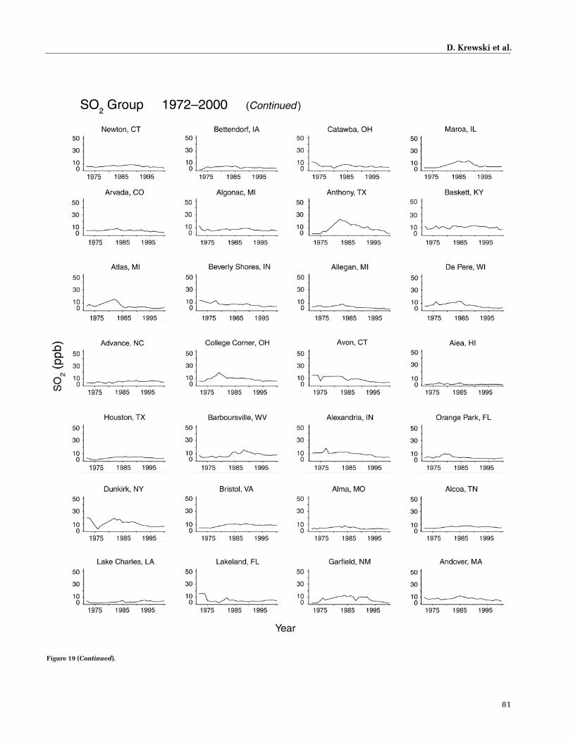
D. Krewski et al.
81
Figure 19 (Continued).

82
Extended Analysis of ACS Study of Particulate Air Pollution and Mortality
Figure 19 (Continued).

D. Krewski et al.
83
Figure 19 (Continued).
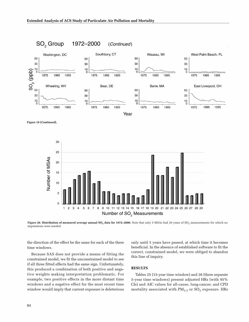
84
Extended Analysis of ACS Study of Particulate Air Pollution and Mortality
Figure 19 (Continued).
Figure 20. Distribution of measured average annual SO2 data for 1972–2000. Note that only 5 MSAs had 29 years of SO2 measurements for which noimputations were needed.
the direction of the effect be the same for each of the threetime windows.
Because SAS does not provide a means of fitting theconstrained model, we fit the unconstrained model to seeif all three fitted effects had the same sign. Unfortunately,this produced a combination of both positive and nega-tive weights making interpretation problematic. Forexample, two positive effects in the more distant timewindows and a negative effect for the most recent timewindow would imply that current exposure is deleterious
only until 5 years have passed, at which time it becomesbeneficial. In the absence of established software to fit thecorrect, constrained model, we were obliged to abandonthis line of inquiry.
RESULTS
Tables 25 (15-year time window) and 26 (three separate5-year time windows) present adjusted HRs (with 95%CIs) and AIC values for all-cause, lung-cancer, and CPDmortality associated with PM2.5 or SO2 exposure. HRs

D. Krewski et al.
85
associated with PM2.5 exposure in several of the 15-yearwindows were elevated, and significantly so for the PM2.5-B cohort group for lung-cancer and CPD mortality. Resultsfor analyses stratified by level of education attainment arepresented in Tables 27–29.
An examination of HRs revealed no clear pattern. ForPM2.5, no one exposure time window stood out as demon-strating the greatest HR; nor was there any clear pattern ofa trend in HRs going from most recent to most distant win-dows or vice versa. For SO2, the HRs were highest in themost recent time window (1 to 5 years), although none ofthe HRs was significantly elevated.
Differences in AIC values among the three 5-year expo-sure time windows were small. For both PM2.5 groups theAIC value tended to be lowest (the model with the best fitto the data) in either the most recent time window (1 to 5years) or the middle time window (6 to 10 years). This wasapparent for all three cause-of-death categories in analyseswith all subjects (Table 26) and in analyses stratified byeducation attainment (Tables 28 and 29). The exceptionwas lung cancer in the PM2.5-A group (Table 26). For theSO2 group, AIC values were lowest in the most recent timewindow for nearly all cause-of-death categories, althoughdifferences in AIC values were again small. The exceptionswere all-cause and lung-cancer mortality among thosewith a lower level of education attainment (Table 28).
DISCUSSION AND CONCLUSIONS
Overall, no clear pattern emerged as to which of the timewindows of exposure may be most responsible for thePM2.5–mortality association. Although for SO2 exposure,models that used exposure data from the most recent 5
years provided a slightly better fit to available data on mor-tality from all causes, lung cancer, and CPD, as evidenced bylower AIC values; these differences were small. The HRs formortality associated with exposure to SO2 were highest inthe most recent time window; however, none of them weresignificantly elevated.
To be able to identify which exposure time windows areassociated with mortality attributable to air pollution, thepatterns of exposure among individuals in the cohort needto be sufficiently varied. Variation can be spatial (differentexposure profiles experienced by individuals living in dif-ferent MSAs) and temporal (exposure profiles for a givenMSA changing over time). In this data set, both spatial andtemporal variations in exposure patterns were limited bythe ecologic nature of the exposure measure used. Greatervariability in temporal exposure patterns may be expectedfor individuals who move from one MSA to another duringthe study period; however, relatively few participantsmoved during the time span of this analysis.
On average, the spatial (between MSAs) and temporal(within MSAs) variations in exposure patterns were sim-ilar for the PM2.5-A group (some of whom moved duringthe study period) and the PM2.5-B group (who wereassumed to not have moved between enrollment anddeath). For spatial variation in both groups, the SD aroundthe annual average PM2.5 concentrations was 5.0; and fortemporal variation it was 3.5 for group A and 3.4 for groupB. Spatial variation of within-MSA temporal variation,however, was somewhat higher in the PM2.5-B group thanin the PM2.5-A group as shown by SDs of 1.9 for group Band 1.7 for group A. For the SO2 group, SDs were 3.7 forspatial variation, 2.6 for temporal variation, and 1.9 forspatial–temporal variation.
Table 25. HRs by Cause of Death Associated with a 10-µg/m3 Change in PM2.5 Concentrations or a 5-ppb Change in SO2 Concentrations Over the 15-Year Time Windowa
Cause of DeathPM2.5-A Group
(n = 60,941)PM2.5-B Group
(n = 81,466)SO2 Group(n = 80,711)
All causesDeaths (n) 6,117 81,466 7,702HR 0.98 (0.92–1.06) 1.01 (0.99–1.02) 0.99 (0.96–1.01)
Lung cancerDeaths (n) 599 6,038 763HR 1.08 (0.87–1.35) 1.07 (1.02–1.13) 0.96 (0.88–1.05)
CPDDeaths (n) 2,478 40,496 3,145HR 1.00 (0.90–1.11) 1.05 (1.03–1.07) 1.01 (0.97–1.05)
a Model included the 44 individual-level covariates. Baseline hazard function was stratified by age (1-year groupings), sex, and race and was adjusted for smoking, marital status, body mass index, alcohol, occupational exposures, and diet. Bolded values refer to text. HRs are followed by 95% confidence intervals.
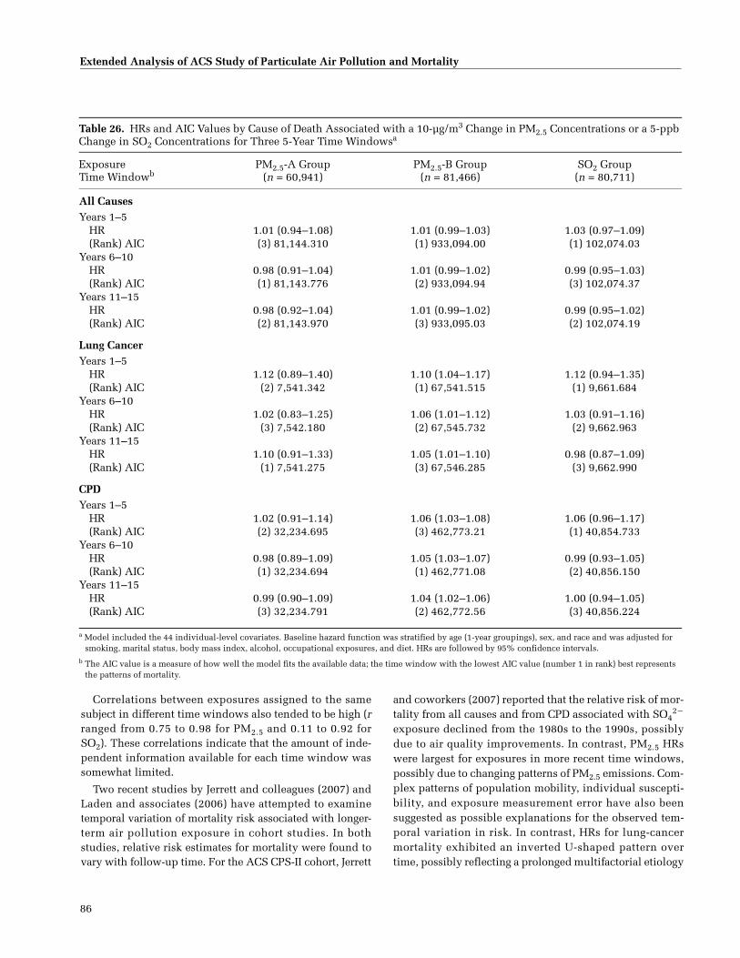
86
Extended Analysis of ACS Study of Particulate Air Pollution and Mortality
Correlations between exposures assigned to the samesubject in different time windows also tended to be high (rranged from 0.75 to 0.98 for PM2.5 and 0.11 to 0.92 forSO2). These correlations indicate that the amount of inde-pendent information available for each time window wassomewhat limited.
Two recent studies by Jerrett and colleagues (2007) andLaden and associates (2006) have attempted to examinetemporal variation of mortality risk associated with longer-term air pollution exposure in cohort studies. In bothstudies, relative risk estimates for mortality were found tovary with follow-up time. For the ACS CPS-II cohort, Jerrett
and coworkers (2007) reported that the relative risk of mor-tality from all causes and from CPD associated with SO4
2�
exposure declined from the 1980s to the 1990s, possiblydue to air quality improvements. In contrast, PM2.5 HRswere largest for exposures in more recent time windows,possibly due to changing patterns of PM2.5 emissions. Com-plex patterns of population mobility, individual suscepti-bility, and exposure measurement error have also beensuggested as possible explanations for the observed tem-poral variation in risk. In contrast, HRs for lung-cancermortality exhibited an inverted U-shaped pattern overtime, possibly reflecting a prolonged multifactorial etiology
Table 26. HRs and AIC Values by Cause of Death Associated with a 10-µg/m3 Change in PM2.5 Concentrations or a 5-ppb Change in SO2 Concentrations for Three 5-Year Time Windowsa
Exposure Time Windowb
PM2.5-A Group(n = 60,941)
PM2.5-B Group(n = 81,466)
SO2 Group(n = 80,711)
All CausesYears 1–5
HR 1.01 (0.94–1.08) 1.01 (0.99–1.03) 1.03 (0.97–1.09)(Rank) AIC (3) 81,144.310 (1) 933,094.00 (1) 102,074.03
Years 6–10HR 0.98 (0.91–1.04) 1.01 (0.99–1.02) 0.99 (0.95–1.03)(Rank) AIC (1) 81,143.776 (2) 933,094.94 (3) 102,074.37
Years 11–15HR 0.98 (0.92–1.04) 1.01 (0.99–1.02) 0.99 (0.95–1.02)(Rank) AIC (2) 81,143.970 (3) 933,095.03 (2) 102,074.19
Lung CancerYears 1–5
HR 1.12 (0.89–1.40) 1.10 (1.04–1.17) 1.12 (0.94–1.35)(Rank) AIC (2) 7,541.342 (1) 67,541.515 (1) 9,661.684
Years 6–10HR 1.02 (0.83–1.25) 1.06 (1.01–1.12) 1.03 (0.91–1.16)(Rank) AIC (3) 7,542.180 (2) 67,545.732 (2) 9,662.963
Years 11–15HR 1.10 (0.91–1.33) 1.05 (1.01–1.10) 0.98 (0.87–1.09)(Rank) AIC (1) 7,541.275 (3) 67,546.285 (3) 9,662.990
CPDYears 1–5
HR 1.02 (0.91–1.14) 1.06 (1.03–1.08) 1.06 (0.96–1.17)(Rank) AIC (2) 32,234.695 (3) 462,773.21 (1) 40,854.733
Years 6–10HR 0.98 (0.89–1.09) 1.05 (1.03–1.07) 0.99 (0.93–1.05)(Rank) AIC (1) 32,234.694 (1) 462,771.08 (2) 40,856.150
Years 11–15HR 0.99 (0.90–1.09) 1.04 (1.02–1.06) 1.00 (0.94–1.05)(Rank) AIC (3) 32,234.791 (2) 462,772.56 (3) 40,856.224
a Model included the 44 individual-level covariates. Baseline hazard function was stratified by age (1-year groupings), sex, and race and was adjusted for smoking, marital status, body mass index, alcohol, occupational exposures, and diet. HRs are followed by 95% confidence intervals.
b The AIC value is a measure of how well the model fits the available data; the time window with the lowest AIC value (number 1 in rank) best represents the patterns of mortality.
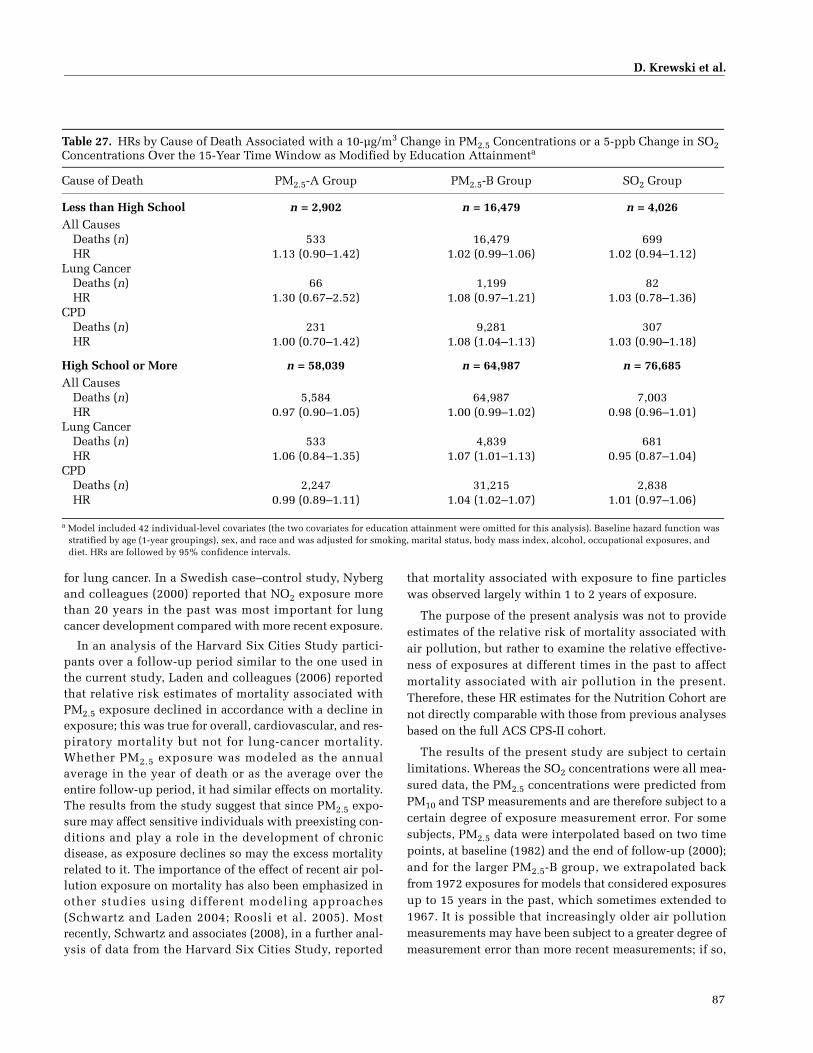
D. Krewski et al.
87
for lung cancer. In a Swedish case–control study, Nybergand colleagues (2000) reported that NO2 exposure morethan 20 years in the past was most important for lungcancer development compared with more recent exposure.
In an analysis of the Harvard Six Cities Study partici-pants over a follow-up period similar to the one used inthe current study, Laden and colleagues (2006) reportedthat relative risk estimates of mortality associated withPM2.5 exposure declined in accordance with a decline inexposure; this was true for overall, cardiovascular, and res-piratory mortality but not for lung-cancer mortality.Whether PM2.5 exposure was modeled as the annualaverage in the year of death or as the average over theentire follow-up period, it had similar effects on mortality.The results from the study suggest that since PM2.5 expo-sure may affect sensitive individuals with preexisting con-ditions and play a role in the development of chronicdisease, as exposure declines so may the excess mortalityrelated to it. The importance of the effect of recent air pol-lution exposure on mortality has also been emphasized inother studies using different modeling approaches(Schwartz and Laden 2004; Roosli et al. 2005). Mostrecently, Schwartz and associates (2008), in a further anal-ysis of data from the Harvard Six Cities Study, reported
that mortality associated with exposure to fine particleswas observed largely within 1 to 2 years of exposure.
The purpose of the present analysis was not to provideestimates of the relative risk of mortality associated withair pollution, but rather to examine the relative effective-ness of exposures at different times in the past to affectmortality associated with air pollution in the present.Therefore, these HR estimates for the Nutrition Cohort arenot directly comparable with those from previous analysesbased on the full ACS CPS-II cohort.
The results of the present study are subject to certainlimitations. Whereas the SO2 concentrations were all mea-sured data, the PM2.5 concentrations were predicted fromPM10 and TSP measurements and are therefore subject to acertain degree of exposure measurement error. For somesubjects, PM2.5 data were interpolated based on two timepoints, at baseline (1982) and the end of follow-up (2000);and for the larger PM2.5-B group, we extrapolated backfrom 1972 exposures for models that considered exposuresup to 15 years in the past, which sometimes extended to1967. It is possible that increasingly older air pollutionmeasurements may have been subject to a greater degree ofmeasurement error than more recent measurements; if so,
Table 27. HRs by Cause of Death Associated with a 10-µg/m3 Change in PM2.5 Concentrations or a 5-ppb Change in SO2 Concentrations Over the 15-Year Time Window as Modified by Education Attainmenta
Cause of Death PM2.5-A Group PM2.5-B Group SO2 Group
Less than High School n = 2,902 n = 16,479 n = 4,026All Causes
Deaths (n) 533 16,479 699HR 1.13 (0.90–1.42) 1.02 (0.99–1.06) 1.02 (0.94–1.12)
Lung CancerDeaths (n) 66 1,199 82HR 1.30 (0.67–2.52) 1.08 (0.97–1.21) 1.03 (0.78–1.36)
CPDDeaths (n) 231 9,281 307HR 1.00 (0.70–1.42) 1.08 (1.04–1.13) 1.03 (0.90–1.18)
High School or More n = 58,039 n = 64,987 n = 76,685All Causes
Deaths (n) 5,584 64,987 7,003HR 0.97 (0.90–1.05) 1.00 (0.99–1.02) 0.98 (0.96–1.01)
Lung CancerDeaths (n) 533 4,839 681HR 1.06 (0.84–1.35) 1.07 (1.01–1.13) 0.95 (0.87–1.04)
CPDDeaths (n) 2,247 31,215 2,838HR 0.99 (0.89–1.11) 1.04 (1.02–1.07) 1.01 (0.97–1.06)
a Model included 42 individual-level covariates (the two covariates for education attainment were omitted for this analysis). Baseline hazard function was stratified by age (1-year groupings), sex, and race and was adjusted for smoking, marital status, body mass index, alcohol, occupational exposures, and diet. HRs are followed by 95% confidence intervals.

88
Extended Analysis of ACS Study of Particulate Air Pollution and Mortality
Table 28. HRs and AIC Values by Cause of Death Associated with a 10-µg/m3 change in PM2.5 Concentrations or a 5-ppb Change in SO2 Concentrations for Three 5-Year Time Windows for Those with an Education of Less than High Schoola
Exposure Time Windowb
PM2.5-A Group(n = 2,902)
PM2.5-B Group(n = 16,479)
SO2 Group(n = 4,026)
All CausesYears 1–5
HR 1.11 (0.87–1.41) 1.03 (0.99–1.07) 1.00 (0.80–1.24)(Rank) AIC (3) 3,930.551 (3) 134,703.47 (3) 5,319.918
Years 6–10HR 1.15 (0.93–1.42) 1.03 (0.996–1.06) 1.04 (0.90–1.19)(Rank) AIC (1) 3,929.531 (1) 134,702.42 (2) 5,319.643
Years 11–15HR 1.10 (0.90–1.33) 1.02 (0.99–1.05) 1.04 (0.92–1.17)(Rank) AIC (2) 3,930.464 (2) 134,703.30 (1) 5,319.545
Lung CancerYears 1–5
HR 1.15 (0.56–2.34) 1.10 (0.97–1.26) 1.12 (0.61–2.04)(Rank) AIC (3) 486.585 (1) 9,346.718 (3) 601.746
Years 6–10HR 1.33 (0.72–2.46) 1.07 (0.96–1.20) 1.12 (0.74–1.69)(Rank) AIC (1) 485.900 (3) 9,347.238 (2) 601.602
Years 11–15HR 1.29 (0.72–2.31) 1.07 (0.98–1.17) 1.18 (0.82–1.71)(Rank) AIC (2) 486.021 (2) 9,346.887 (1) 601.098
CPDYears 1–5
HR 1.10 (0.76–1.60) 1.09 (1.04–1.14) 1.08 (0.77–1.50)(Rank) AIC (1) 1,689.729 (3) 76,074.461 (1) 2,354.605
Years 6–10HR 0.99 (0.71–1.38) 1.08 (1.04–1.13) 1.01 (0.82–1.25)(Rank) AIC (3) 1,690.004 (1) 76,071.375 (3) 2,354.778
Years 11–15HR 0.94 (0.69–1.28) 1.07 (1.03–1.10) 0.97 (0.80–1.17)(Rank) AIC (2) 1,689.836 (2) 76,072.491 (2) 2,354.686
a Model included 42 individual-level covariates (the two covariates for education attainment were omitted for this analysis). Baseline hazard function was stratified by age (1-year groupings), sex, and race and was adjusted for smoking, marital status, body mass index, alcohol, occupational exposures, and diet. HRs are followed by 95% confidence intervals.
b The AIC value is a measure of how well the model fits the available data; the time window with the lowest AIC value (number 1 in rank) best represents the patterns of mortality.
that could result in higher AIC values and a bias of HRstoward the null in more distant exposure time windows.
We may have also misclassified exposure with certainassumptions about individuals’ residential histories, suchas that the place of residence remained unchanged before1982. The PM2.5-B group was composed entirely of partic-ipants who had died and were assumed to have nevermoved, whereas the PM2.5-A and SO2 groups were com-posed of self-selected CPS-II participants who had sur-
vived until 1992. Although this may introduce some typeof a selection bias, we think it does not influence the iden-tification of critical exposure time windows, which aredetermined by the pathophysiological disease processes.
Updated information for certain demographic and life-style covariates have been collected in follow-up surveysfor Nutrition Cohort participants. Although data on thesecovariates were not available for all study participantsincluded in this analysis, most of the covariates do not

D. Krewski et al.
89
Table 29. HRs and AIC Values by Cause of Death Associated with a 10-µg/m3 Change in PM2.5 Concentrations or a 5-ppb Change in SO2 Concentrations for Three 5-Year Time Windows for Those with an Education of High School or Morea
Exposure Time Windowb
PM2.5-A Group(n = 58,039)
PM2.5-B Group(n = 64,987)
SO2 Group(n = 76,685)
All CausesYears 1–5
HR 1.00 (0.93–1.08) 1.01 (0.99–1.03) 1.03 (0.96–1.10)(Rank) AIC (3) 73,721.769 (1) 722,351.83 (1) 92,415.750
Years 6–10HR 0.96 (0.90–1.03) 1.00 (0.98–1.02) 0.99 (0.95–1.03)(Rank) AIC (1) 73,720.383 (3) 722,352.50 (3) 92,416.128
Years 11–15HR 0.97 (0.91–1.03) 1.00 (0.99–1.02) 0.99 (0.95–1.02)(Rank) AIC (2) 73,720.888 (2) 722,352.49 (2) 92,416.016
Lung CancerYears 1–5
HR 1.12 (0.87–1.42) 1.10 (1.03–1.18) 1.13 (0.93–1.37)(Rank) AIC (1) 6,702.496 (1) 52,588.969 (1) 8,620.221
Years 6–10HR 0.99 (0.79–1.23) 1.06 (1.00–1.12) 1.04 (0.91–1.18)(Rank) AIC (3) 6,703.257 (2) 52,592.574 (3) 8,621.479
Years 11–15HR 1.08 (0.88–1.33) 1.05 (0.998–1.10) 0.96 (0.86–1.08)(Rank) AIC (2) 6,702.698 (3) 52,593.565 (2) 8,621.350
CPDYears 1–5
HR 1.01 (0.90–1.14) 1.05 (1.02–1.08) 1.06 (0.96–1.18)(Rank) AIC (2) 29,075.089 (1) 346,041.73 (1) 36,658.773
Years 6–10HR 0.98 (0.88–1.09) 1.04 (1.02–1.07) 0.99 (0.93–1.06)(Rank) AIC (1) 29,074.988 (2) 346,042.27 (2) 36,660.093
Years 11–15HR 0.99 (0.90–1.10) 1.04 (1.01–1.06) 1.00 (0.95–1.06)(Rank) AIC (3) 29,075.102 (3) 346,043.24 (3) 36,660.141
a Model included 42 individual-level covariates (the two covariates for education attainment were omitted for this analysis). Baseline hazard function was stratified by age (1-year groupings), sex, and race and was adjusted for smoking, marital status, body mass index, alcohol, occupational exposures, and diet. HRs are followed by 95% confidence intervals.
b The AIC value is a measure of how well the model fits the available data; the time window with the lowest AIC value (number 1 in rank) best represents the patterns of mortality.
appreciably affect the air pollution–mortality relationship(education attainment is the major exception) and werenot expected to complicate the identification of criticaltime windows of exposure (Krewski et al. 2000a,b). In thepresent study, stratification of the analysis by level of edu-cation attainment (less than high school versus highschool or greater) did not shed light on the question ofwhich time windows might be most important. However,consistent with previous studies that did not account forresidential mobility information, we also observed larger
mortality HRs among those with a lower level of educationattainment. Levels of smoking cessation may have also dif-fered between analytic groups.
Overall, identification of critical exposure time win-dows, even among large national cohorts, remains a chal-lenge and further research to identify them with otherrelevant data sets is needed. Such work would improveour understanding of the time frame surrounding thehuman health benefits from reduced exposure to long-termair pollution.

90
Extended Analysis of ACS Study of Particulate Air Pollution and Mortality
IMPLICATIONS OF THE FINDINGS
PHASE I
This report provides the results of Phase III of the Par-ticle Epidemiology Reanalysis Project, which began in1998. Phases I and II together are referred to as the Reanal-ysis. In Phase I, we validated the data used in the HarvardSix Cities Study (follow-up 1974–1991; Dockery et al.1993) and the American Cancer Society Study (follow-up1982–1989; Pope et al. 1995) of long-term exposure to par-ticulate air pollution and mortality and, using the sameanalytic methods, replicated the numerical resultsreported by the original investigators. Our findings inPhase I established the integrity of the original data andconfirmed, with trivial discrepancies, the original risk esti-mates (Krewski et al. 2000a; 2003b; 2004; 2005a).
PHASE II
In Phase II, we conducted a detailed sensitivity analysisto assess the robustness of the original findings to alterna-tive analytic approaches (Krewski et al. 2000b). Specificsensitivity analyses focused on the impact on risk estimates
of including additional individual-level covariates in therisk models that relate particulate air pollution with mor-tality; including new ecologic covariates related to demo-graphic factors, socioeconomic indicators, availability ofhealth services, climate variables, characteristics of thephysical environment, and gaseous copollutants (Krewskiet al. 2000b; 2003a,b); possible confounding due to occu-pational exposures (Siemiatycki et al. 2003); and popula-tion mobility.
These sensitivity analyses produced four main results:(1) Adjusting for most ecologic covariates did not substan-tially alter mortality risk estimates related to exposure toparticulate and gaseous air pollutants. An exception waspopulation change (movement of people from one area ofthe country to another), which notably reduced the risk esti-mates for all-cause mortality related to SO4
2� exposure,although the effects of population change were completelyattenuated by control for residual autocorrelation. (2) Therisk estimates did not vary with adjustment for most indi-vidual-level covariates. However, education attainment wasfound to modify the effect — risk estimates for all causes ofdeath studied decreased with increasing education attain-ment for both PM2.5 and SO4
2� exposures. (3) Adjustmentfor ambient SO2 concentrations at the MSA scale markedly
Figure 21. Spatial distribution (kriged) of PM2.5 concentrations based on data from 1982–1986. Analysis done in Phase II (Krewski et al. 2000b).
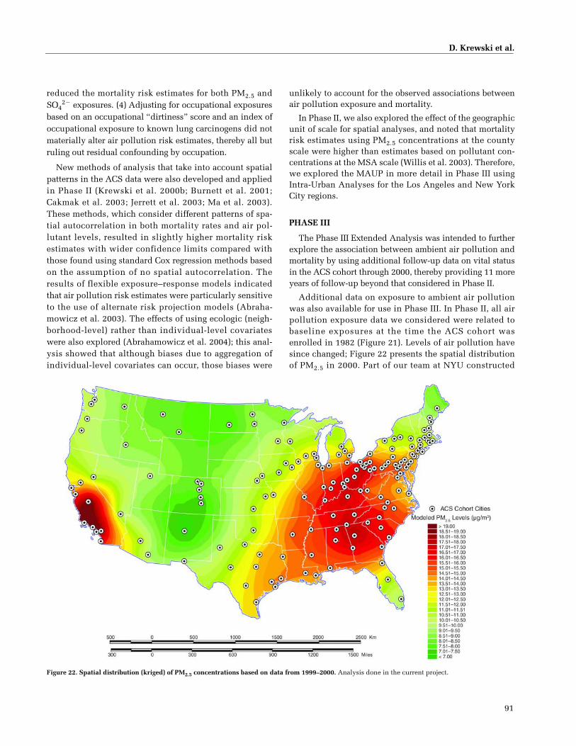
D. Krewski et al.
91
Figure 22. Spatial distribution (kriged) of PM2.5 concentrations based on data from 1999–2000. Analysis done in the current project.
reduced the mortality risk estimates for both PM2.5 andSO4
2� exposures. (4) Adjusting for occupational exposuresbased on an occupational “dirtiness” score and an index ofoccupational exposure to known lung carcinogens did notmaterially alter air pollution risk estimates, thereby all butruling out residual confounding by occupation.
New methods of analysis that take into account spatialpatterns in the ACS data were also developed and appliedin Phase II (Krewski et al. 2000b; Burnett et al. 2001;Cakmak et al. 2003; Jerrett et al. 2003; Ma et al. 2003).These methods, which consider different patterns of spa-tial autocorrelation in both mortality rates and air pol-lutant levels, resulted in slightly higher mortality riskestimates with wider confidence limits compared withthose found using standard Cox regression methods basedon the assumption of no spatial autocorrelation. Theresults of flexible exposure–response models indicatedthat air pollution risk estimates were particularly sensitiveto the use of alternate risk projection models (Abraha-mowicz et al. 2003). The effects of using ecologic (neigh-borhood-level) rather than individual-level covariateswere also explored (Abrahamowicz et al. 2004); this anal-ysis showed that although biases due to aggregation ofindividual-level covariates can occur, those biases were
unlikely to account for the observed associations betweenair pollution exposure and mortality.
In Phase II, we also explored the effect of the geographicunit of scale for spatial analyses, and noted that mortalityrisk estimates using PM2.5 concentrations at the countyscale were higher than estimates based on pollutant con-centrations at the MSA scale (Willis et al. 2003). Therefore,we explored the MAUP in more detail in Phase III usingIntra-Urban Analyses for the Los Angeles and New YorkCity regions.
PHASE III
The Phase III Extended Analysis was intended to furtherexplore the association between ambient air pollution andmortality by using additional follow-up data on vital statusin the ACS cohort through 2000, thereby providing 11 moreyears of follow-up beyond that considered in Phase II.
Additional data on exposure to ambient air pollutionwas also available for use in Phase III. In Phase II, all airpollution exposure data we considered were related tobaseline exposures at the time the ACS cohort wasenrolled in 1982 (Figure 21). Levels of air pollution havesince changed; Figure 22 presents the spatial distributionof PM2.5 in 2000. Part of our team at NYU constructed

92
Extended Analysis of ACS Study of Particulate Air Pollution and Mortality
annual average estimates of PM2.5 concentrations for1972–2000, and we used them in the analysis of possiblecritical exposure time windows. Measured annual averageSO2 concentrations were also available from the EPA AIRSdatabase for the same period.
The specific objectives of Phase III were threefold: (1)Do social, economic, and demographic ecologic variablesconfound or modify the relationship between particulateair pollution and mortality? (2) How can spatial autocorre-lation and multiple geographic levels be taken intoaccount within the random effects Cox models? (3) Whatcritical exposure time windows affect the associationbetween air pollution and mortality?
During the course of Phase III, a fourth objective offocusing on Intra-Urban Analyses in the Los Angeles andNew York City regions was added. These Intra-Urban Anal-yses were intended to explore the MAUP by using moregeographically refined indicators of air pollution exposure.Specifically, the relatively dense grid of air pollution mon-itors in both of these large cities permitted an assessment ofexposure to ambient air pollution at the ZCA scale.
The extensive series of analyses conducted during thecourse of Phase III provided a number of important find-ings concerning the association between exposure toambient air pollutants and mortality.
SUMMARY OF RESULTS FROM PHASE III
Nationwide Analysis
The first set of analyses focused on further character-izing the relationship between air pollution and mortalityusing the most recent follow-up data for the ACS cohort.
Nationwide Analysis of the full ACS cohort confirmedthat mortality increases with exposure to PM2.5; the HR fordeath from all causes was 1.033 (95% CI, 1.015–1.052), fordeath from CPD was 1.091 (95% CI, 1.063–1.120), fordeath from IHD was 1.152 (95% CI, 1.111–1.196), and fordeath from lung cancer was 1.110 (95% CI, 1.040–1.185)(see Table 3). These risk estimates were based on annualaverage air pollutant concentrations in 1999–2000 and werecalculated based on a 10-µg/m3 change in PM2.5. (Similaralthough slightly lower risk estimates were obtained usingair pollutant concentrations for 1979–1983.)
The Reanalysis showed stronger and more robustassociations between SO2 exposure and all causes of mor-tality compared with those observed for PM2.5 exposure(Krewski et al. 2000b). A plausible mechanism by whichSO2 could increase mortality risk, however, has not yet beenidentified. One possibility is that SO2 may serve as a markerfor particulate air pollution formed by the atmospheric
transformation of SO2 into SO42� particles. In contrast, the
present analysis showed stronger mortality associationsfor PM2.5 than for SO2 exposure. We did not investigatesources of particles or particle transformation; however,source apportionment is an important avenue for futureresearch.
In analyses conducted at the national level, the largestmortality risk estimates were consistently associated withIHD; a similar result was noted in the Reanalysis Project.Whereas lung-cancer mortality in Phase II was found notto be significantly elevated in relation to PM2.5 exposure,the additional number of lung-cancer deaths during thefurther 11 years of follow-up used for Phase III resulted ina significant association between PM2.5 exposure and lungcancer. A significant increase in lung-cancer mortality wasalso noted in the Updated Analysis of the ACS cohort withfollow-up through 1998 (Pope et al. 2002).
We adjusted models for ecologic covariates to accountfor sociodemographic risks, which would yield less biasedmortality risk estimates of air pollution exposure. In nearlyall models that adjusted for the seven ecologic covariatessimultaneously, the HR tended to increase in comparisonto models with no adjustment, although many of the differ-ences were small. The geographic unit of analysis of eco-logic covariates (ZCA, MSA, or MSA & DIFF) tended not tomake an appreciable difference in influence on HR esti-mates; however, in many cases HR estimates tended to behighest in models with the ecologic covariates consideredat the MSA & DIFF levels simultaneously.
The air pollution–lung-cancer mortality associationwas also found to vary somewhat by the level of educationattainment recorded when subjects were enrolled. Specif-ically, participants who completed high school or less hada significant increase in risk of lung-cancer mortality ofapproximately 20% associated with each 10-µg/m3 changein PM2.5 (as measured in 2000) compared with no associ-ation observed for those who completed more than highschool.
Intra-Urban Analyses
The Intra-Urban Analyses for the Los Angeles regionusing the LUR-based exposure assignments resulted innotably larger mortality risk estimates than those found inthe Nationwide Analysis. Such differences were suggestedby an earlier simulation study of the effects of exposuremeasurement error in studies of this type conducted byMallick and associates (2002). Mortality risk estimatesusing the LUR-based exposure estimates were somewhatsmaller than those based on the exposure estimates fromthe kriging model, but were generally comparable. The HRof mortality due to exposure to PM2.5 in Los Angeles from
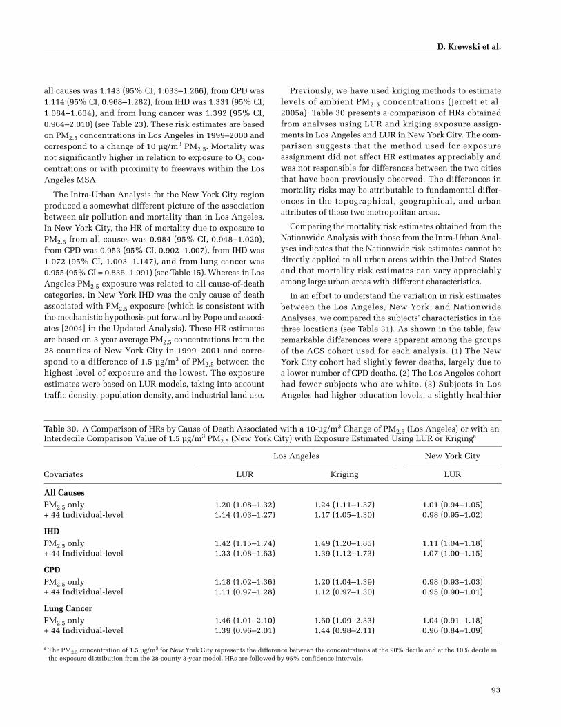
D. Krewski et al.
93
all causes was 1.143 (95% CI, 1.033–1.266), from CPD was1.114 (95% CI, 0.968–1.282), from IHD was 1.331 (95% CI,1.084–1.634), and from lung cancer was 1.392 (95% CI,0.964–2.010) (see Table 23). These risk estimates are basedon PM2.5 concentrations in Los Angeles in 1999–2000 andcorrespond to a change of 10 µg/m3 PM2.5. Mortality wasnot significantly higher in relation to exposure to O3 con-centrations or with proximity to freeways within the LosAngeles MSA.
The Intra-Urban Analysis for the New York City regionproduced a somewhat different picture of the associationbetween air pollution and mortality than in Los Angeles.In New York City, the HR of mortality due to exposure toPM2.5 from all causes was 0.984 (95% CI, 0.948–1.020),from CPD was 0.953 (95% CI, 0.902–1.007), from IHD was1.072 (95% CI, 1.003–1.147), and from lung cancer was0.955 (95% CI = 0.836–1.091) (see Table 15). Whereas in LosAngeles PM2.5 exposure was related to all cause-of-deathcategories, in New York IHD was the only cause of deathassociated with PM2.5 exposure (which is consistent withthe mechanistic hypothesis put forward by Pope and associ-ates [2004] in the Updated Analysis). These HR estimatesare based on 3-year average PM2.5 concentrations from the28 counties of New York City in 1999–2001 and corre-spond to a difference of 1.5 µg/m3 of PM2.5 between thehighest level of exposure and the lowest. The exposureestimates were based on LUR models, taking into accounttraffic density, population density, and industrial land use.
Previously, we have used kriging methods to estimatelevels of ambient PM2.5 concentrations (Jerrett et al.2005a). Table 30 presents a comparison of HRs obtainedfrom analyses using LUR and kriging exposure assign-ments in Los Angeles and LUR in New York City. The com-parison suggests that the method used for exposureassignment did not affect HR estimates appreciably andwas not responsible for differences between the two citiesthat have been previously observed. The differences inmortality risks may be attributable to fundamental differ-ences in the topographical, geographical, and urbanattributes of these two metropolitan areas.
Comparing the mortality risk estimates obtained from theNationwide Analysis with those from the Intra-Urban Anal-yses indicates that the Nationwide risk estimates cannot bedirectly applied to all urban areas within the United Statesand that mortality risk estimates can vary appreciablyamong large urban areas with different characteristics.
In an effort to understand the variation in risk estimatesbetween the Los Angeles, New York, and NationwideAnalyses, we compared the subjects' characteristics in thethree locations (see Table 31). As shown in the table, fewremarkable differences were apparent among the groupsof the ACS cohort used for each analysis. (1) The NewYork City cohort had slightly fewer deaths, largely due toa lower number of CPD deaths. (2) The Los Angeles cohorthad fewer subjects who are white. (3) Subjects in LosAngeles had higher education levels, a slightly healthier
Table 30. A Comparison of HRs by Cause of Death Associated with a 10-µg/m3 Change of PM2.5 (Los Angeles) or with an Interdecile Comparison Value of 1.5 µg/m3 PM2.5 (New York City) with Exposure Estimated Using LUR or Kriginga
Covariates
Los Angeles New York City
LUR Kriging LUR
All CausesPM2.5 only 1.20 (1.08–1.32) 1.24 (1.11–1.37) 1.01 (0.94–1.05)+ 44 Individual-level 1.14 (1.03–1.27) 1.17 (1.05–1.30) 0.98 (0.95–1.02)
IHDPM2.5 only 1.42 (1.15–1.74) 1.49 (1.20–1.85) 1.11 (1.04–1.18)+ 44 Individual-level 1.33 (1.08–1.63) 1.39 (1.12–1.73) 1.07 (1.00–1.15)
CPDPM2.5 only 1.18 (1.02–1.36) 1.20 (1.04–1.39) 0.98 (0.93–1.03)+ 44 Individual-level 1.11 (0.97–1.28) 1.12 (0.97–1.30) 0.95 (0.90–1.01)
Lung CancerPM2.5 only 1.46 (1.01–2.10) 1.60 (1.09–2.33) 1.04 (0.91–1.18)+ 44 Individual-level 1.39 (0.96–2.01) 1.44 (0.98–2.11) 0.96 (0.84–1.09)
a The PM2.5 concentration of 1.5 µg/m3 for New York City represents the difference between the concentrations at the 90% decile and at the 10% decile in the exposure distribution from the 28-county 3-year model. HRs are followed by 95% confidence intervals.

94
Extended Analysis of ACS Study of Particulate Air Pollution and Mortality
diet, and higher levels of alcohol consumption. (4) Occu-pational exposures were slightly lower in Los Angelesand New York than in the national cohort. (5) With theexception of a lower proportion of white subjects, theslight differences of the characteristics in the Los Angelescohort compared with the New York cohort were likely toincrease survival, which would likely decrease suscepti-bility to air pollution; yet the health effects observed in LosAngeles were generally higher than those observed ineither of the other two groups. Based on these compari-sons, it appears unlikely that the differences in resultsobserved between the Nationwide Analysis and the twoIntra-Urban Analyses are attributable to differences in the
underlying characteristics in each cohort group. The possi-bility of confounding by non-PM effects of mobile sources,such as noise, remains.
Critical Exposure Time Windows
A unique aspect of Phase III was the use of the ACSNutrition Cohort to examine the time window of exposurethat may be primarily responsible for the associationbetween air pollution and mortality. We constructed anindividual time-dependent exposure profile for each par-ticipant in this large cohort for which population mobilityinformation was available. We evaluated air pollutantexposure concentrations experienced by individuals
Table 31. Descriptive Statistics of Risk Factors for the Nationwide, New York City, and Los Angeles Data Sets
Variable Nationwidea New York City Los Angeles
Participants (n) 488,370 44,056 22,905Participants died from (%)
All causes 26.4 24.0 25.6CPD 13.1 10.5 13.7Lung cancer 2.0 1.9 1.9All other causes 11.3 11.1 10.0
Ageb 56.6 (10.5) 55.3 (10.7) 57.0 (10.6)Male (%) 56.5 56.3 57.0White (%) 94.0 95.0 89.1
Education (%)< High School 12.1 11.8 8.2High School 31.2 31.2 22.9> High School 56.7 57.0 68.9
Current Smoker (%) 21.9 23.5 19.3Cigarettes per day 22.0 (12.4) 21.8 (12.6) 21.3 (12.6)Years of smoking 33.6 (11.0) 32.8 (11.0) 34.0 (11.1)
Former smoker (%) 30.3 33.5 33.0Cigarettes per day 21.6 (14.6) 22.1 (15.1) 20.9 (14.8)Years of smoking 22.2 (4.1) 25.2 (4.0) 24.7 (4.0)
Age when started smoking (%)< 18 yrs (current smoker) 9.3 11.5 8.4� 18 yrs (current smoker) 13.0 12.4 11.3< 18 yrs (former smoker) 11.8 15.3 12.0� 18 yrs (former smoker) 18.4 18.3 20.8
Hours per day exposed to smokingb 3.2 (4.4) 3.6 (4.5) 2.8 (4.2)
Table continues next page
a Based on the 116 MSAs for which PM2.5 (1999–2000) data were available in the national dataset and follow-up of participants through 2000.b Mean (SD).c Occupational exposure to PM increases with increasing index number.d Dietary fat consumption increases with increasing index number.e Dietary fiber consumption increases with increasing index number.

D. Krewski et al.
95
dynamically, during three separate exposure time win-dows reflecting individual exposure 1–5, 6–10, and 11–15years in the past. Overall, no clear findings emerged foreither PM2.5 or SO2. Identification of critical exposure timewindows, even among large national cohorts, remains achallenge and further work on identifying them with otherrelevant datasets — including other cohorts with differentexposure circumstances — is needed.
REVISIONS TO THE COX MODELS
An important methodologic contribution from Phase IIIis the extension of the random effects Cox regression
models to handle multiple levels of clustering. The soft-ware developed for this purpose in Phase II has been sig-nificantly enhanced and allows for a broader class ofspatial autocorrelation models. We expect the extendedrandom effects Cox regression model software to findapplication in a wide variety of research directions outsideof the ACS cohort.
Application of the random effects Cox model to theupdated ACS cohort data in Phase III tended to modestlyincrease the air pollution risk estimates over those fromthe standard Cox model, and to inflate the uncertainty inthe estimates, as is reflected in the associated broader con-fidence limits.
Table 31 (Continued). Descriptive Statistics of Risk Factors for the Nationwide, New York City, and Los Angeles Data Sets
Variable Nationwidea New York City Los Angeles
Marital status (%)Married 83.9 83.0 80.9Separated 3.5 4.5 3.6Divorced 12.6 12.5 15.5
Body mass indexb 25.2 (4.1) 25.2 (4.0) 24.7 (4.0)
Occupational exposure to PM indexc (%)Level 1 13.1 13.9 13.1Level 2 11.3 10.2 12.4Level 3 4.7 4.5 4.6Level 4 6.4 4.9 3.8Level 5 4.2 3.7 4.1Level 6 1.1 0.6 0.8Not able to access 8.7 10.1 9.2
Self-reported exposure to dust or fumes (%) 19.9 19.2 19.5
Dietary fat consumption indexd (%)Level 1 15.9 18.2 17.8Level 2 17.5 18.6 18.3Level 3 21.4 21.5 21.3Level 4 30.9 25.2 24.5
Dietary fiber consumption indexe (%)Level 1 19.8 20.0 18.1Level 2 18.8 19.3 17.4Level 3 22.8 23.3 22.9Level 4 22.0 21.2 26.4
Alcohol consumption (%)Drink beer 22.9 23.2 22.4Drink liquor 27.6 30.4 31.3Drink wine 23.2 29.9 34.2
a Based on the 116 MSAs for which PM2.5 (1999–2000) data were available in the national dataset and follow-up of participants through 2000.b Mean (SD).c Occupational exposure to PM increases with increasing index number.d Dietary fat consumption increases with increasing index number.e Dietary fiber consumption increases with increasing index number.

96
Extended Analysis of ACS Study of Particulate Air Pollution and Mortality
COMPARISON OF DATA SETS AND ANALYTIC METHODS FOR THE THREE FOLLOW-UP TIME PERIODS
We further examined how a variety of analytic factorsmay influence the estimation of the long-term air pollu-tion–mortality association in the ACS cohort over time.Table 32 provides some descriptive statistics about threemajor analyses conducted with the ACS cohort data at dif-ferent points in time.
In the Reanalysis Project (Krewski et al. 2000b), PM2.5exposure data were available for the time period 1979–1983 for 50 MSAs containing 298,825 study participants.Follow-up of participants had been performed through1989 and had documented a total of 23,180 deaths from allcauses, 11,262 from CPD, 2,001 from lung cancer, and5,968 from IHD.
In the Updated Analysis by Pope and colleagues (2002),the follow-up period had been extended by 9 years until1998. Additional PM2.5 data had been obtained and expo-sure could be estimated for two time periods (1979–1983and 1999–2000); these corresponded to a total of 61 and 116MSAs, respectively. Due in large part to the longer follow-up period, more deaths had occurred; over 80,000 deathsfrom all causes were recorded among those subjects forwhom PM2.5 exposure data for 1979–1983 were available.
Finally, for the current Extended Analysis, the ACSfollow-up period had been extended by 2 more years,until 2000. Because we examined several additional eco-logic covariates at different levels of analysis, the total
number of MSAs and participants available for theNationwide Analysis was slightly lower than the numberavailable for the Updated Analysis by Pope and col-leagues (2002). The two additional years of follow-up,however, included more deaths: over 90,000 from allcauses among the same group for whom PM2.5 exposuredata were available for 1979–1983.
Table 33 compares HR estimates for the five main cause-of-death categories using different cohort follow-upperiods (until 1989, 1998, and 2000) that correspond withthe analytic time periods used for the Reanalysis Project(Krewski et al. 2000a,b), the Updated Analysis (Pope et al.2002), and the current Extended Analysis. By holding thenumber of MSAs and study subjects constant, we werebetter able to examine the independent influence ofchanging the length of the follow-up period on study find-ings. The PM2.5 (1979–1983) results were obtained usingavailable data for 342,521 subjects residing in 58 MSAs,and the PM2.5 (1999–2000) results were obtained usingavailable data for 488,370 subjects residing in 116 MSAs.Results are presented with adjustment for the standardsuite of 44 individual-level covariates and with andwithout adjustment for the seven ecologic covariatesexamined in the current study.
With models adjusted for individual-level covariatesonly, estimated HRs associated with exposure to PM2.5(1979–1983) ranged from 1.03–1.05 for all causes, 1.07–1.10for CPD, 1.12–1.13 for IHD, and 1.05–1.09 for lung cancer.HR estimates were slightly higher for IHD and lung cancer
Table 32. Characteristics of the Analytic Cohorts in the Previous and Current Analysesa
Characteristic
Cohort Data Set Used in
Reanalysis (2000)
Cohort Data Sets Used in
Updated Analysis(2002, 2004)
Cohort Data SetsUsed in
Current Nationwide Analysis (2009)
Years of PM2.5 exposure data 1979–1983 1979–1983 1999–2000 1979–1983 1999–2000Years of cohort follow-up 1982–1989 1982–1998 1982–1998 1982–2000 1982–2000MSAs (n) 50 61 116 58 116Study participants (n) 298,825 360,682 499,779b 342,521 488,370b
Person-years 2,109,750 5,302,337 7,350,011 5,542,998 7,908,283Deaths (n)
All causes 23,180 80,819 111,677 90,783 128,954CPD 11,262 35,782 49,539 44,866 63,917Lung cancer 2,001 6,335 8,754 6,827 9,788IHD 5,968 14,691 20,791 20,651 29,989
a Bolded data refer to text.b For the PM2.5 1999–2000 exposure data, the 116 MSAs used for the Updated Analysis and in the current Nationwide Analysis are the same. The number
of study participants differs because several additional ecologic covariates were analyzed in the current study and those data were not available for the full cohort.

D. Krewski et al.
97
associated with the PM2.5 (1999–2000) exposure data. Withmodels including ecologic covariates, HR estimatesincreased to 1.04–1.06 for all causes, 1.09–1.13 for CPD,1.18 for IHD, and 1.07–1.10 for lung-cancer mortality asso-ciated with exposure to PM2.5 (1979–1983) over the dif-ferent follow-up time periods. Overall, there was littlechange in risk estimates over different periods of follow-up time; those for PM2.5 (1979–1983) tended to eitherremain fairly similar or decrease slightly with increasingfollow-up time. An exception was lung-cancer mortalityfor which HRs increased and were significant whenfollow-up was extended beyond 1989.
It is possible that there may be increasing exposuremisclassification due to population mobility during the11 years of follow-up from 1989 to 2000. A recent anal-ysis by Jerrett and colleagues (2007) showed that popula-tion mobility in the ACS cohort demonstrates that areas
of relatively low improvements in air pollution havehigher population gains.
Table 34 shows the influence of (1) the number of MSAsand participants included in the analysis and (2) thechoice of statistical method (either the standard Cox modelor the random effects Cox model). For these analyses, weeither held the number of MSAs and participants constantacross the different follow-up periods (using the samenumber of MSAs and participants as those in the currentstudy) or we allowed the number of MSAs and partici-pants to vary across the different follow-up periods (usingthe number of MSAs and participants that correspondedwith those used in the earlier analyses [Krewski et al.2000a,b; Pope et al. 2002; see Table 32]). For PM2.5 (1979–1983) both the number of MSAs and participants couldvary; but for PM2.5 (1999–2000), the number of MSAs was
Table 33. HRs by Cause of Death for a 10-µg/m3 Change in PM2.5 Covering Three Follow-Up Time Periods, Using the Same Number of MSAs and Study Participants Within PM2.5 Exposure Categories, and With and Without Adjustment for the Seven Ecologic Covariatesa
Covariatesin Modelb
Follow-Up Through 1989
Follow-Up Through 1998
Follow-Up Through 2000
PM2.5 1979–1983 1979–1983 1999–2000 1979–1983 1999–2000MSAs (n) 58 58 116 58 116Participants (n) 342,521 342,521 488,370 342,521 488,370
All Causes44 Individual 1.048 (1.022–1.076) 1.031 (1.015–1.047) 1.032 (1.012–1.053) 1.028 (1.014–1.043) 1.036 (1.017–1.054)+ 7 Ecologic 1.061 (1.031–1.091) 1.047 (1.029–1.064) 1.057 (1.033–1.080) 1.044 (1.028–1.060) 1.057 (1.036–1.079)
CPD44 Individual 1.101 (1.061–1.143) 1.071 (1.048–1.095) 1.092 (1.063–1.123) 1.070 (1.049–1.092) 1.100 (1.073–1.129)+ 7 Ecologic 1.129 (1.084–1.175) 1.098 (1.073–1.125) 1.134 (1.099–1.170) 1.094 (1.070–1.118) 1.138 (1.106–1.172)
IHD44 Individual 1.122 (1.066–1.181) 1.130 (1.094–1.166) 1.143 (1.099–1.190) 1.133 (1.100–1.167) 1.155 (1.113–1.199)+ 7 Ecologic 1.183 (1.119–1.250) 1.183 (1.143–1.225) 1.234 (1.179–1.291) 1.184 (1.146–1.222) 1.242 (1.191–1.295)
Lung Cancer44 Individual 1.053 (0.963–1.150) 1.089 (1.031–1.151) 1.116 (1.041–1.197) 1.075 (1.021–1.132) 1.109 (1.039–1.185)+ 7 Ecologic 1.070 (0.973–1.177) 1.104 (1.040–1.171) 1.152 (1.065–1.247) 1.092 (1.033–1.154) 1.138 (1.057–1.225)
All Other Causes44 Individual 0.998 (0.958–1.040) 0.981 (0.957–1.005) 0.953 (0.924–0.982) 0.979 (0.957–1.000) 0.953 (0.927–0.980)+ 7 Ecologic 0.992 (0.949–1.037) 0.984 (0.958–1.010) 0.953 (0.920–0.988) 0.983 (0.960–1.007) 0.953 (0.923–0.984)
a Based on a standard Cox model with the 44 individual-level covariates with and without adjustment for the seven ecologic covariates at MSA & DIFF levels. The baseline hazard function was stratified by age (1-year groupings), gender, and race. All analyses were conducted using the same 58 MSAs (342,521 participants) or 116 MSAs (488,370 participants) that were used in the current analysis. HRs are followed by 95% confidence intervals. Bolded data refer to text.
b Data for the 44 individual-level covariates are from the ACS enrollment questionnaire. Data for the seven ecologic covariates were extracted from the 1980 U.S. Census Bureau database for the Nationwide Analysis of the current study.

98
Extended Analysis of ACS Study of Particulate Air Pollution and Mortality
Table 34. HRs by Cause of Death for a 10-µg/m3 Change in PM2.5 Based on Either a Standard Cox or a Random Effects Cox Model Covering Three Follow-Up Time Periods and Using the Same or Different Numbers of MSAs and Participantsa
Model and Number of MSAs
Follow-UpThrough 1989b
Follow-UpThrough 1998c
Follow-UpThrough 2000d
PM2.5 data 1979–1983 1979–1983 1999–2000 1979–1983 1999–2000Samee
MSAs (n) 58 58 116 58 116Participants (n) 342,521 342,521 488,370 342,521 488,370
Differente
MSAs (n) 50 61 116 58 116Participants (n) 298,825 360,682 499,779 342,521 488,370
All Causes Standard Cox
Same 1.048 (1.022–1.076) 1.031 (1.015–1.047) 1.032 (1.012–1.053) 1.028 (1.014–1.043) 1.036 (1.017–1.054)Different 1.067 (1.037–1.099) 1.027 (1.012–1.043) 1.028 (1.009–1.048)
Random Effects CoxSame 1.074 (1.028–1.122) 1.046 (1.014–1.080) 1.061 (1.023–1.101) 1.042 (1.012–1.073) 1.063 (1.026–1.102)Different 1.101 (1.046–1.157) 1.044 (1.011–1.078) 1.058 (1.020–1.098)
CPD Standard Cox
Same 1.101 (1.061–1.143) 1.071 (1.048–1.095) 1.092 (1.063–1.123) 1.070 (1.049–1.092) 1.100 (1.073–1.129)Different 1.109 (1.063–1.157) 1.060 (1.036–1.084) 1.079 (1.049–1.111)
Random Effects CoxSame 1.116 (1.055–1.180) 1.075 (1.032–1.120) 1.100 (1.044–1.159) 1.073 (1.031–1.116) 1.105 (1.050–1.162)Different 1.130 (1.063–1.201) 1.061 (1.018–1.105) 1.081 (1.025–1.141)
IHD Standard Cox
Same 1.122 (1.066–1.181) 1.130 (1.094–1.166) 1.143 (1.099–1.190) 1.133 (1.100–1.167) 1.155 (1.113–1.199)Different 1.122 (1.059–1.189) 1.119 (1.081–1.159) 1.141 (1.091–1.193)
Random Effects CoxSame 1.167 (1.062–1.282) 1.160 (1.074–1.252) 1.198 (1.099–1.305) 1.155 (1.074–1.124) 1.200 (1.106–1.301)Different 1.174 (1.064–1.295) 1.140 (1.053–1.235) 1.192 (1.085–1.310)
Lung Cancer Standard Cox
Same 1.053 (0.963–1.150) 1.089 (1.031–1.151) 1.116 (1.041–1.197) 1.075 (1.021–1.132) 1.109 (1.039–1.185)Different 1.001 (0.907–1.104) 1.072 (1.017–1.130) 1.117 (1.042–1.197)
Random Effects CoxSame 1.117 (0.979–1.274) 1.102 (1.032–1.177) 1.129 (1.045–1.220) 1.085 (1.019–1.156) 1.124 (1.041–1.213)Different 1.062 (0.913–1.235) 1.083 (1.014–1.157) 1.126 (1.044–1.214)
All Other Causes Standard Cox
Same 0.998 (0.958–1.040) 0.981 (0.957–1.005) 0.953 (0.924–0.982) 0.979 (0.957–1.000) 0.953 (0.927–0.980)Different 1.040 (0.993–1.089) 0.992 (0.971–1.013) 0.971 (0.944–0.998)
Random Effects CoxSame 1.017 (0.960–1.077) 1.001 (0.961–1.043) 0.991 (0.946–1.039) 0.999 (0.962–1.037) 0.963 (0.879–1.055) Different 1.063 (0.995–1.135) 1.014 (0.975–1.054) 1.010 (0.967–1.055)
a Models included the 44 individual-level covariates. The baseline hazard function was stratified by age (1-year groupings), gender, and race. HRs are followed by 95% confidence intervals. Bolded values refer to text.
b Follow-up period used for the Reanalysis Project (Krewski et al. 2000).c Follow-up period used for the Updated Analysis (Pope et al. 2002, 2004).d Follow-up period used for this Extended Analysis. e Rows marked “Same” use the MSAs and participants from the current Nationwide Analysis. Rows marked “Different” use the MSAs and participants
included in the earlier analyses (as outlined in Table 32).
D. Krewski et al.
99
the same in both follow-up periods, and only the numberof participants varied.
As noted previously, risk estimates obtained with therandom effects Cox model were slightly higher than thoseobtained with the standard Cox model; the comparisons inTable 34 show this pattern fairly consistently.
In results obtained with the standard Cox model, therewas only slight variation in the mortality HR estimates com-paring calculations with the same number or differentnumber of MSAs and participants. One of the largestchanges in the HRs was found for mortality from lung-cancer associated with PM2.5 (1979–1983) with follow-upthrough 1989 with a HR of 1.00 (95% CI, 0.91–1.10) whenusing data from 50 MSAs (“different” row), which increasedto 1.05 (95% CI, 0.96–1.15) when we included the 8 addi-tional MSAs for which PM2.5 data had later been obtained(“same” row), although it remained nonsignificant.
A similar pattern was observed with the random effectsCox model. Again, the difference in risk estimates wasslight whether using the same number or a differentnumber of MSAs and participants. The largest differencewas also observed for mortality from lung cancer associ-ated with PM2.5 (1979–1983) with follow-up through 1989with a HR of 1.062 (95% CI, 0.913–1.235) found whenusing data from 50 MSAs (“different” row), whichincreased, although again remained nonsignificant, to1.117 (95% CI, 0.979–1.274) reported when we included 8additional MSAs (“same” row).
Table 35 presents a comparison of the modifying effectof education attainment on the association between PM2.5(1979–1983) and mortality over the three follow-up timeperiods with and without the ecologic covariates exam-ined as part of the Nationwide Analysis. (Note that this setof analyses uses the same 58 MSAs and 342,521 subjects asthe current Extended Analysis.) In the two most recentperiods (through 1998 and 2000), risk of mortalitydecreased with increasing level of education attainmentfor all-cause and cause-specific mortality and, with theexception of IHD, was no longer significant in those withthe highest level of education attainment. When thefollow-up time period was truncated at 1989, although thedecreasing trend was less clear, the lowest risk estimateswere also consistently reported in the highest educationgroup. A similar pattern of results was obtained with orwithout adjustment for the seven ecologic covariates eval-uated in the current study.
POLICY IMPLICATIONS
The results of Phase III of the Particle EpidemiologyReanalysis Project have important implications for air
quality risk management policy. The extended follow-upof the ACS cohort through 2000 supports earlier findingsof a positive association between long-term exposure toPM2.5 in ambient air and increased mortality rates in urbancenters in the United States. The earlier results have fig-ured prominently in establishing the current NationalAmbient Air Quality Standard for PM2.5 in the UnitedStates (U.S. EPA 2004). Although short-term exposures toPM2.5 are also associated with higher mortality, one of theeffects of long-term exposure (Cohen et al. 2003) is to pre-dispose some people to the effects attributed to short-termexposures (Network for Environmental Risk Assessmentand Management [NERAM] 2002; Krewski et al. 2005b).
Particulate air pollution represents a major health issueat the international level as well (Cohen et al. 2005). TheWorld Health Organization (WHO 2002) has estimated thatparticulate air pollution is responsible for approximately2% of all deaths worldwide. WHO has assumed a leader-ship role in global air quality management and hasrecently updated its air quality guidelines for both PM2.5and O3 (WHO 2006).
Although the precise magnitude of the risk associatedwith long-term exposure to air pollution remains subject tosome uncertainty, these and earlier results from the ACScohort have generally demonstrated elevated mortalityfrom CPD, IHD, and lung cancer. Mortality from all causesis also clearly associated with long-term exposure toambient PM2.5 in U.S. urban centers. Phases II and III ofthe Particle Epidemiology Reanalysis Project have bothshown these estimates to be robust to alternative analyticmethods and to adjustment for other variables that mayimpact the association between air pollution and mortality.
In an attempt to address the uncertainty about the actualmagnitude of the increase in mortality due to long-termexposure to fine particles, the U.S. EPA has recently con-ducted an expert elicitation involving leading researchersin the health effects of air pollution, especially those withexperience evaluating data from large cohorts includingthe ACS, the Harvard Six Cities Study (Laden et al. 2006),and the Adventist Health Study of Smog (Abbey et al.1999). This expert elicitation process demonstrated a clearconsensus among the participating scientists that long-term exposure to particulate air pollution is associatedwith increased mortality (Industrial Economics, Incorpo-rated 2006).
The policy implications of the current body of scientificevidence linking air pollution to morbidity and mortalitywere recently discussed at the fifth and final NERAMCollo-quium on Air Quality and Health (NERAM 2006).Whereas NERAM I (Cohen et al. 2003), II (Krewski et al.2005a), and III (Craig et al. 2007) focused more on the

100
Extended Analysis of ACS Study of Particulate Air Pollution and Mortality
Tabl
e 35
.M
odif
icat
ion
by
Ed
uca
tion
Att
ain
men
t: H
Rs
by C
ause
of
Dea
th f
or a
10-
µg/
m3 C
han
ge i
n P
M2.
5 (1
979–
1983
) C
over
ing
Th
ree
Fol
low
-Up
Tim
e P
erio
ds,
Wit
h a
nd
Wit
hou
t S
even
Eco
logi
cal
Cov
aria
tes,
an
d U
sin
g th
e S
ame
Nu
mbe
r of
MS
As
and
Stu
dy
Par
tici
pan
tsa
Lev
el o
fE
du
cati
onF
ollo
w-U
pT
hro
ugh
198
9F
ollo
w-U
pT
hro
ugh
199
8F
ollo
w-U
pT
hro
ugh
200
0
Cov
aria
tesb
42 I
nd
ivid
ual
+ 7
Eco
logi
c42
In
div
idu
al+
7 E
colo
gic
42 I
nd
ivid
ual
+ 7
Eco
logi
c
All
Cau
ses
< H
igh
sch
ool
1.08
1 (1
.024
–1.1
40)
1.10
4 (1
.042
–1.1
70)
1.07
4 (1
.038
–1.1
12)
1.09
9 (1
.059
–1.1
41)
1.07
2 (1
.038
–1.1
07)
1.09
5 (1
.058
–1.1
34)
Hig
h s
choo
l1.
092
(1.0
42–1
.145
)1.
090
(1.0
36–1
.147
)1.
050
(1.0
21–1
.079
)1.
065
(1.0
33–1
.097
)1.
045
(1.0
18–1
.071
)1.
057
(1.0
29–1
.087
)>
Hig
h s
choo
l1.
007
(0.9
69–1
.046
)1.
016
(0.9
74–1
.060
)1.
001
(0.9
79–1
.023
)1.
011
(0.9
87–1
.036
)1.
000
(0.9
80–1
.021
)1.
011
(0.9
89–1
.034
)
CP
D<
Hig
h s
choo
l1.
103
(1.0
27–1
.185
)1.
122
(1.0
38–1
.213
)1.
125
(1.0
74–1
.178
)1.
154
(1.0
98–1
.213
)1.
129
(1.0
81–1
.178
)1.
157
(1.1
04–1
.212
)H
igh
sch
ool
1.15
3 (1
.075
–1.2
36)
1.18
4 (1
.099
–1.2
75)
1.10
3 (1
.060
–1.1
48)
1.13
2 (1
.084
–1.1
82)
1.08
7 (1
.048
–1.1
28)
1.11
2 (1
.069
–1.1
57)
>H
igh
sch
ool
1.06
6 (1
.007
–1.1
27)
1.08
9 (1
.023
–1.1
58)
1.02
4 (0
.992
–1.0
57)
1.04
2 (1
.006
–1.0
80)
1.02
9 (1
.000
–1.0
60)
1.04
4 (1
.011
–1.0
79)
IHD
<H
igh
sch
ool
1.14
8 (1
.040
–1.2
68)
1.18
9 (1
.068
–1.3
24)
1.18
3 (1
.106
–1.2
64)
1.22
9 (1
.144
–1.3
21)
1.18
2 (1
.110
–1.2
60)
1.22
4 (1
.143
–1.3
11)
Hig
h s
choo
l1.
170
(1.0
64–1
.286
)1.
232
(1.1
14–1
.362
)1.
173
(1.1
07–1
.242
)1.
219
(1.1
46–1
.296
)1.
153
(1.0
93–1
.216
)1.
195
(1.1
29–1
.266
)>
Hig
h s
choo
l1.
070
(0.9
91–1
.156
)1.
133
(1.0
41–1
.232
)1.
073
(1.0
24–1
.125
)1.
129
(1.0
72–1
.188
)1.
093
(1.0
47–1
.142
)1.
149
(1.0
95–1
.205
)
Lu
ng
Can
cer
<H
igh
sch
ool
1.09
5 (0
.911
–1.3
17)
1.11
5 (0
.912
–1.3
63)
1.17
5 (1
.034
–1.3
35)
1.18
6 (1
.034
–1.3
60)
1.15
5 (1
.024
–1.3
02)
1.14
2 (1
.004
–1.2
98)
Hig
h s
choo
l1.
196
(1.0
22–1
.400
)1.
189
(1.0
03–1
.409
)1.
151
(1.0
47–1
.267
)1.
163
(1.0
49–1
.288
)1.
152
(1.0
54–1
.259
)1.
168
(1.0
61–1
.286
)>
Hig
h s
choo
l0.
931
(0.8
15–1
.064
)0.
992
(0.8
60–1
.144
)1.
012
(0.9
35–1
.096
)1.
040
(0.9
54–1
.135
)0.
993
(0.9
21–1
.070
)1.
028
(0.9
48–1
.116
)
All
Oth
er C
ause
s<
Hig
h s
choo
l1.
046
(0.9
54–1
.148
)1.
085
(0.9
83–1
.198
)0.
995
(0.9
39–1
.055
)1.
015
(0.9
52–1
.081
)0.
987
(0.9
35–1
.042
)1.
008
(0.9
50–1
.070
)H
igh
sch
ool
1.02
1 (0
.949
–1.0
98)
0.98
9 (0
.914
–1.0
70)
0.98
1 (0
.940
–1.0
25)
0.98
1 (0
.936
–1.0
28)
0.98
6 (0
.948
–1.0
26)
0.98
4 (0
.943
–1.0
27)
>H
igh
sch
ool
0.97
2 (0
.917
–1.0
30)
0.95
6 (0
.896
–1.0
19)
0.97
8 (0
.945
–1.0
11)
0.97
7 (0
.941
–1.0
15)
0.97
3 (0
.943
–1.0
03)
0.97
5 (0
.942
–1.0
09)
a B
ased
on
a s
tan
dar
d C
ox m
odel
wit
h 4
2 in
div
idu
al-l
evel
cov
aria
tes.
Th
e ba
seli
ne
haz
ard
fu
nct
ion
was
str
atif
ied
by
age
(1-y
ear
grou
pin
gs),
gen
der
, an
d r
ace.
HR
s ar
e fo
llow
ed b
y 95
% c
onfi
den
ce
inte
rval
s. A
ll a
nal
yses
wer
e co
nd
uct
ed u
sin
g th
e sa
me
58 M
SA
s an
d 3
42,5
21 p
arti
cip
ants
use
d i
n t
he
curr
ent
Ext
end
ed A
nal
ysis
.b D
ata
for
the
42 i
nd
ivid
ual
-lev
el c
ovar
iate
s ar
e fr
om t
he
AC
S e
nro
llm
ent
ques
tion
nai
re. D
ata
for
the
seve
n e
colo
gic
cova
riat
es (
at M
SA
& D
IFF
lev
els)
wer
e ex
trac
ted
fro
m t
he
1980
U.S
. Cen
sus
Bu
reau
dat
abas
e fo
r th
e N
atio
nw
ide
Aan
alys
is i
n t
he
curr
ent
stu
dy.

D. Krewski et al.
101
scientific evidence of the adverse health effects of ambientair pollution, NERAM IV (2005) and V (2006) focused on airquality management. The conference statement for NERAMV includes the following policy guidelines:
1. Current scientific evidence on adverse health impactsis sufficient to support air quality management action.
2. Air quality management actions have been shown tobe cost-beneficial in a number of circumstances.
3. Although additional scientific evidence will be usefulin targeted areas, such as characterizing the effects oftraffic-related pollution, air quality managementactions are needed now.
4. Successful air quality management requires local,regional, national, international, and global actions.
The results of the present analysis support the call forgreater efforts to reduce exposure to air pollution embod-ied in the NERAM V conference statement. In developingair quality management policy, the following additionalelements of the NERAM V conference statement are alsorelevant.
1. Harmonization of air quality measurement methodsand health assessments is desirable.
2. Different air quality management strategies may beneeded for developed and developing countries.
3. Air quality and climate change are closely linked.
4. Cross-sectoral strategies (air, climate, transportation,energy, agriculture) based on integrated assessmentsare needed.
5. Air quality management strategies should supportsustainable development.
6. The impact of air quality management interventionsneeds to be evaluated.
The accountability framework proposed by the HEIAccountability Working Group (2003) provides an excel-lent basis for addressing the last item.
In conclusion, Phase III of the Particle EpidemiologyReanalysis Project has provided additional support for thedevelopment of effective air quality management policiesand strategies. The epidemiologic results reported here areconsistent with those from other population-based studies,which collectively support the hypothesis that long-termexposure to PM2.5 increases mortality in the general popu-lation. We also now know mechanisms by which particlescan increase mortality from CPD (Pope et al. 2004;National Research Council 2004), which provides a bio-logic basis for the associations observed.
ACKNOWLEDGMENTS
The authors would like to thank the following individ-uals for their contributions to the study: Huixia Jiang forproviding programming support, Lorraine Craig for edito-rial assistance, and Dan Crouse, Karen King, and RichardHamilton for assistance with statistical analyses, cartog-raphy, and graphic design. The following individuals con-tributed to the New York City Intra-Urban Analysis: Dr.John Mbwana, Cornell University, assisted with traffic dataanalysis; Michael Chiume, Sangeeta Bhowmick, and AlanGershowitz, NYMTC, prepared traffic data.
Finally, the authors would like to acknowledge projectfunding support from the following sponsors: HealthEffects Institute, the National Institute of EnvironmentalHealth Sciences (Grants 5 R01 ES 09560, 5 P30 ES07048,5P01ES011627, 5P01 ES11627, 5P01 ES09581), the Cali-fornia Air Resources Board (Grant 55245A), and the U.S.EPA (RD-83184501-0, RD-8318610-1). Additional supportwas provided through the Verna Richter Chair in CancerResearch (Duncan Thomas).
REFERENCES
Abbey DE, Nishino N, McDonnell WF, Burchette RJ,Knutsen SF, Beeson WL, Yang JX. 1999. Long-term inhal-able particles and other air pollutants related to mortalityin nonsmokers. Am J Respir Crit Care Med 159:373–382.
Abrahamowicz M, Du Berger R, Krewski K, Burnett R,Bartlett G, Tamblyn RM, Leffondre K. 2004. Bias due toaggregation of individual covariates in the Cox regressionmodel. Am J Epidemiol 160:696–706.
Abrahamowicz M, Schopflocher T, Leffondre K, du BergerR, Krewski D. 2003. Flexible modeling of exposure-response relationship between long-term average levels ofparticulate air pollution and mortality in the AmericanCancer Society study. J Toxicol Environ Health A 66:1625–1654.
Amrhein C, Reynolds H. 1997. Using the Getis statistic toexplore aggregation effects in metropolitan Toronto censusdata. The Canadian Geographer 41:137–149.
Armstrong DL, Strogatz D, Barnett E, Wang R. 2003. Jointeffects of social class and community occupational struc-ture on coronary mortality among black men and whitemen, upstate New York, 1988-92. J Epidemiol CommunityHealth 57:373–378.
102
Extended Analysis of ACS Study of Particulate Air Pollution and Mortality
Bailey TC, Gatrell AC. 1995. Interactive Spatial Data Anal-ysis. John Wiley and Sons, New York, NY.
Bari A, Ferraro V, Wilson L, Luttinger D, Husain L. 2003.Measurement of gaseous HONO, HNO3, SO2, HCL, NH3,particulate sulfate and PM2.5 in New York, NY. AtmosEnviron 37:2825–2835.
Bay Area Air Quality Management District [BAAQMD].2005. Climate, physiography and air pollution potential:Bay area and its subregions. Bay Area Air Quality Manage-ment District, San Francisco, CA.
Bell ML, McDermott A, Zeger SL, Samet JM, Dominici F.2004. Ozone and short-term mortality in 95 U.S. urbancommunities, 1987–2000. JAMA 292:2372–2378.
BoundarySeer User Guide. 2001. Biomedware, Ann Arbor,MI.
Boyd C, Zhang-Salomons JY, Groome PA, Mackillop WJ.1999. Associations between community income andcancer survival in Ontario, Canada, and the United States.J Clin Oncol 17:2244–2255.
Brauer M, Hoek G, van Vliet P, Meliefste K, Fischer P,Brunekreef B. 2002. Air pollution from traffic and thedevelopment of respiratory infections and asthmatic andallergic symptoms in children. Am J Respir Crit Care Med166:1092–1098.
Brauer M, Hoek G, van Vliet P, Meliefste K, Fischer P,Gehring U, Heinrich J, Cyrys J, Bellander T, Lewne M,Brunekreef B. 2003. Estimating long-term average particu-late air pollution concentrations: Application of trafficindicators and geographic information systems. Epidemi-ology 14:228–239.
Briggs D, de Hoogh C, Gulliver J, Wills J, Elliott P, KinghamS, Smallbone K. 2000a. A regression-based method formapping traffic-related air pollution: Application andtesting in four contrasting urban environments. Sci TotalEnviron 253:151–167.
Briggs D, Paul E, Shaddick G, Fraser A. 2000b. Changinggeographic relationships between air pollution and cardio-respiratory mortality in Great Britain, 1962-1996. Epidemi-ology 11:S103–S103.
Brook RD, Franklin B, Cascio W, Hong Y, Howard G,Lipsett M, Luepker R, Mittleman M, Samet J, Smith SC Jr,Tager I, Expert Panel on Population and Prevention Sci-ence of the American Heart Association. 2004. Air pollu-tion and cardiovascular disease. A statement forhealthcare professionals from the expert panel on Popula-
tion and Prevention Science of the American Heart Associ-ation. Circulation 109:2655–2671.
Brunekreef B. 1997. Air pollution and life expectancy: Isthere a relation? Occup Environ Med 54:781–784.
Brunekreef B, Holgate S. 2002. Air pollution and health.Lancet 360:1233–1242.
Burnett R, Ma R, Jerrett M, Goldberg MS, Cakmak S, PopeCA III, Krewski D. 2001. The spatial association betweencommunity air pollution and mortality: A new method ofanalyzing correlated geographic cohort data. EnvironHealth Perspect 109:375–380.
Burnham KP, Anderson DR. 2002. Model Selection andMultimodel Inference: A Practical-Theoretic Approach,2nd ed. Springer-Verlag, New York, NY.
Burrough PA, McDonnell RA. 1998. Principals of Geo-graphical Information Systems. Oxford University Press,Oxford.
Cakmak SR, Burnett T, Jerrett M, Goldberg MS, Pope C III,Ma R, Gultekin T, Thun MJ, Krewski D. 2003. Spatialregression models for large-cohort studies linking commu-nity air pollution and health. J Toxicol Environ Part HealthA 66:1811–1823.
Calle EE, Rodriguez C, Jacobs EJ, Almon ML, Chao A,McCullough ML, Feigelson HS, Thun MJ. 2002. The Amer-ican Cancer Society Cancer Prevention Study II NutritionCohort: Rationale, study design, and baseline characteris-tics. Cancer 94:2490–2501.
Calle EE, Terrell DD. 1993. Utility of the National DeathIndex for ascertainment of mortality among Cancer Pre-vention Study II participants. Am J Epidemiol 137:235–241.
California Environmental Protection Agency and AirResources Board. 2003. 2002 California PM2.5 monitorynetwork description. R. Rothacker, California Environ-ment Protection Agency: 76.
Chen LHY, Shao Q. 2004. Normal approximation underlocal dependence. Ann Probab 32:1985–2028.
Christakos G, Serre ML. 2003. Efficient mapping of Cali-fornia mortality fields at different spatial scales. J ExposAnal Environ Epidemiol 13:120–133.
City of New York Department of City Planning. 2009.DCPLION. Available from http://home2.nyc.gov/html/dcp/html/bytes/meta_lion.shtml. Last updated Sep-tember 2008.
D. Krewski et al.
103
Cohen AJ, Krewski D, Samet J, Willes R (eds.). 2003. Healthand air quality: Interpreting science for decision makers. JToxicol Environ Health Part A 66:1489–1903.
Cohen AJ, Ross Anderson H, Ostro B, Pandey KD, Krzyza-nowski M, Künzli N, Gutschmidt, K, Pope A, Romieu I,Samet JM, Smith K. 2005. The global burden of disease dueto outdoor air pollution. J Toxicol Environ Health A68:1301–1307.
Cooper RS, Kennelly JF, Durazo-Arvizu R, Oh HJ, KaplanG, Lynch J. 2001. Relationship between premature mor-tality and socioeconomic factors in black and white popu-lations of U.S. metropolitan areas. Public Health Rep116:464–473.
Cox DR. 1972. Regression models and life tables (with Dis-cussion). J R Stat Soc Ser B 55:187–220.
Cox DR, Oakes D. 1984. Analysis of Survival Data, p. 103.Chapman and Hall, New York.
Craig L, Krewski D, Samet J, Shortreed J, van Bree L. 2007.Strategies for clean air and health. J Toxicol EnvironHealth A 70:183–364.
Crowder MJ. 1986. On consistency and inconsistency ofestimating equations. Econometrics Theory 3:305–330.
Crowder MJ. 1987. On linear and quadratic estimatingfunction. Biometrika 74:591–597.
Curtis S, Taket A. 1996. Health and Societies: ChangingPerspectives. Edward Arnold, London.
Cutter SL, Holm D, Clark L. 1996. The role of geographicscale in monitoring environmental justice. Risk Anal16:517–526.
DeGaetano A, Doherty O. 2004. Temporal, spatial andmeteorological variations in hourly PM2.5 concentrationextremes in New York City. Atmos Environ 38:1547–1558.
Diez Roux AV. 2002. A glossary for multilevel analysis. JEpidemiol Community Health 56:588–594.
Dockery DW, Pope CA III, Xu X, Spengler JD, Ware JH, FayME, Ferris BG, Speizer FE. 1993. An association betweenair pollution and mortality in six U.S. cities. N Engl J Med329:1753–1759.
Duncan C, Jones K, Moon G. 1996. Health-related behav-iour in context: A multi-level modeling approach. Soc SciMed 42: 817–830.
ESRI. 2004. Deterministic Methods for Spatial Interpola-tion. Environmental Systems Research Institute, Redlands,California, USA.
Evans GW, Kantrowitz E. 2002. Socioeconomic status andhealth: The potential role of environmental risk exposure.Annu Rev Public Health 23:303–331.
Eyles J. 1999. Health, environmental assessment and pop-ulation health: Tools for a complex process. Can J PublicHealth 90:S31–S34.
Fotheringham AS, Brunsdon C, Charlton M. 2000. Quanti-tative Geography: Perspectives on Spatial Data Analysis.Thousand Oaks: Sage Publications, London.
Gamble JF. 1998. PM2.5 and mortality in long-term pro-spective cohort studies: Cause-effect or statistical associa-tions? Environ Health Perspect 106:535–549.
Gauderman WJ, Avol E, Gilliland F, Vora H, Thomas D,Berhane K, McConnell R, Künzli N, Lurmann F, RappaportE, Margolis H, Bates D, Peters J. 2004. The effect of air pol-lution on lung development from 10 to 18 years of age. NEngl J Med 351:1057–1067.
Gilbert NL, Goldberg MS, Beckerman B, Brook JR, JerrettM. 2005. Assessing spatial variability of ambient nitrogendioxide in Montreal, Canada, with a land-use regressionmodel. J Air Waste Manage Assoc 55:1059–1063.
Gilliland F, Avol E, Kinney P, Jerrett M, Dvonch T,Lurmann F, Buckley T, Breysse P, Keeler G, de Villiers T,McConnell R. 2005. Air pollution exposure assessment forepidemiologic studies of pregnant women and children:Lessons learned from the Centers for Children's Environ-mental Health and Disease Prevention Research. EnvironHealth Perspect 113:1447–1454.
Goddard MJ, Murdoch DJ, Krewski D. 1995. Temporalaspects of risk characterization. Inhal Toxicol 7:1005–1018.
Goldberg MS, Bailar JC III, Burnett R, Brook J, Tamblyn R,Bonvalot Y, Ernst P, Flegel KM, Singh R, Valois MF. 2000.Identifying subgroups of the general population that maybe susceptible to short-term increases in particulate airpollution: A time series study in Montreal, Quebec.Research Report 97. Health Effects Institute, Cambridge,MA.
Goldberg MS, Burnett R, Bailar JC III, Brook J, Bonvalot Y,Tamblyn R, Singh R, Valois MF. 2001a. The associationbetween daily mortality and short-term effects of ambientair particulate pollution in Montreal, Quebec: 1. Nonacci-dental mortality. Environ Res 86:12–25.
Goldberg MS, Burnett R, Bailar JC III, Brook J, Bonvalot Y,Tamblyn R, Singh R, Valois MF, Vincent R. 2001b. Theassociation between daily mortality and short-term effects
104
Extended Analysis of ACS Study of Particulate Air Pollution and Mortality
of ambient air particle pollution in Montreal, Quebec: 2.Cause-specific mortality. Environ Res 86:26–36.
Gordon P, Richardson H. 1996. Beyond polycentricity thedispersed metropolis, Los Angeles, 1970-1990. J Am PlannAssoc 62:289–295.
Greenberg M. 1993. Proving environmental inequity insiting locally unwanted land uses. Risk Issues Health Saf4:235–252.
Hansen KA. 1998. Seasonality of moves and duration ofresidence. U.S. Census Bureau Report. Curr Popul Rep p.70–66.
He X, Shao Q. 2000. On parameters of increasing dimen-sion. J Multivar Anal 73:120–135.
HEI Accountability Working Group. 2003. AssessingHealth Impact of Air Quality Regulations: Concepts andMethods for Accountability Research. Communication 11.Health Effects Institute, Boston, MA.
HEI Health Review Committee. 2000. Commentary. In:Reanalysis of the Harvard Six Cities Study and the Amer-ican Cancer Society Study of Particulate Air Pollution andMortality (Krewski D, Burnett R, Goldberg M, Hoover K,Siemiatycki J, Jerrett M, Abrahamowicz M, White W).Health Effects Institute, Cambridge, MA.
Hochadel M, Heinrich J, Gehring U, Morgenstern V,Kuhlbusch T, Link E, Wichmann HE, Krämer U. 2006. Pre-dicting long-term average concentrations of traffic relatedair pollutants using GIS-based information. AtmosEnviron 40:542–553.
Hoek G, Brunekreef B, Goldbohm S, Fischer P, van denBrandt PA. 2002. Association between mortality and indi-cators of traffic-related air pollution in The Netherlands: Acohort study. Lancet 360:1203–1209.
Hosmer W, Lemeshow S. 1999. Applied Survival Analysis.Wiley and Sons, New York, NY.
Hricko, A. 2004. Road to an unhealthy future for SouthernCalifornia's children. University of Southern CaliforniaUrban Initiative, p. 1–11.
Industrial Economics, Incorporated. 2006. Expandedexpert judgment assessment of the concentration-responserelationship between PM2.5 exposure and mortality. FinalReport. Available from: www.epa.gov/ttn/ecas/regdata/Uncertainty/pm_ee_report.pdf (Accessed January 3, 2008).
Janssen N, van Vliet P, Aarts F, Harssema H, Brunekreef B.2001. Assessment of exposure to traffic related air pollu-tion of children attending schools near motorways. AtmosEnviron 35:3875–3884.
Jerrett M, Arain A, Kanaroglou P, Beckerman B, PotoglouD, Sahsuvaroglu T, Korrison J, Giovis C. 2005a. A reviewand evaluation of intraurban air pollution exposuremodels. J Expo Anal Environ Epidemiol 15:185–204.
Jerrett M, Burnett RT, Kanaroglou P, Eyles J, Finkelstein N,Giovis C, Brook J. 2001. A GIS-environmental justice anal-ysis of particulate air pollution in Hamilton, Canada.Environ Plan A 33:955–973.
Jerrett M, Burnett RT, Ma RJ, Pope CA 3rd, Krewski D,Newbold KB, Thurston G, Shi YL, Finkelstein N, Calle EE,Thun MJ. 2005b. Spatial analysis of air pollution and mor-tality in Los Angeles. Epidemiology 16:727–736.
Jerrett M, Burnett R, Willis A, Krewski D, Goldberg MS,DeLuca PF, Finkelstein N. 2003. Spatial analysis of the airpollution mortality relationship in the context of ecologicconfounders. J Toxicol Environ Health 66:1735–1777.
Jerrett M, Eyles J, Cole D, Reader S. 1997. Environmentalequity in Canada: An empirical investigation into theincome distribution of pollution in Ontario. Environ PlanA 29:1777–1800.
Jerrett M, Newbold KB, Burnett RT, Thurston G, Lall R,Pope CA III, Ma R, DeLuca P, Thun M, Calle EE, Krewski D.2007. Geographies of uncertainty in the health benefits ofair quality improvements. Stoch Environ Res Risk Assess21:511–522.
Jørgensen B, Knudsen SJ. 2004. Parameter orthogonalityand bias adjustment for estimating functions. Scand J Stat31:93–114.
Jørgensen B, Lundbye-Christensen S, Song X-K, Sun L.1996. A longitudinal study of emergency room visits andair pollution for Prince George, British Columbia. Stat Med15 23–836.
Kaplan GA, Pamuk ER, Lynch JW, Cohen RD, Balfour JL.1996. Inequality in income and mortality in the UnitedStates: Analysis of mortality and potential pathways. BMJ312:999–1003.
Krewski D, Burnett RT, Goldberg MS, Abrahamowicz M,Siemiatycki J, Jerrett M, Hoover K. 2003a. Rejoinder:Reanalysis of the Harvard six cites study and AmericanCancer Society study of particulate air pollution and mor-tality. J Toxicol Environ Health Part A 66:1715–1722.

D. Krewski et al.
105
Krewski D, Burnett RT, Goldberg MS, Hoover K, Siemi-atycki J, Abrahamowicz M, White WH. 2000a. Part I: Rep-lication and Validation. In: Reanalysis of the Harvard SixCities Study and the American Cancer Society Study ofParticulate Air Pollution and Mortality. A Special Reportof the Institute's Particle Epidemiology Reanalysis Project.Health Effects Institute, Cambridge, MA.
Krewski D, Burnett RT, Goldberg MS, Hoover BK, Siemi-atycki J, Abrahamowicz M, White WH. 2004. Validation ofthe Harvard six cities study of air pollution and mortality.N Engl J Med 350:198–199.
Krewski D, Burnett RT, Goldberg MS, Hoover K, Siemi-atycki J, Jerrett M, Abrahamowicz M, White WH. 2000b.Part II. Sensitivity Analysis. In: Reanalysis of the HarvardSix Cities Study and the American Cancer Society Study ofParticulate Air Pollution and Mortality. A Special Reportof the Institute's Particle Epidemiology Reanalysis Project.Health Effects Institute, Cambridge, MA.
Krewski D, Burnett RT, Goldberg MS, Hoover K, Siemi-atycki J, Jerrett M, Abrahamowicz M, White WH. 2003b.Overview of the reanalysis of the Harvard Six Cities studyand American Cancer Society study of particulate air pol-lution and mortality. J Toxicol Environ Health A 66:1507–1552.
Krewski D, Burnett R, Jerrett M, Pope CA III, Rainham D,Calle E, Thurston G, Thun G. 2005a. Mortality and long-term exposure to ambient air pollution: Ongoing analysesbased on the American Cancer Society Cohort. J ToxicolEnviron Health A 68:1093–1109.
Krewski D, Samet JM, Craig L (eds.). 2005b. Interpretingepidemiologic studies of acute and long-term exposure toparticulate matter for policy development. J ToxicolEnviron Health A 68:1049–1307.
Krieger N, Chen JT, Waterman PD, Soobader MJ, Subrama-nian SV, Carson R. 2002. Geocoding and monitoring ofU.S. socioeconomic inequalities in mortality and cancerincidence: Does the choice of area-based measure and geo-graphic level matter? The public health disparities geoc-oding project. Am J Epidemiol 156:471–482.
Kunst AE, Groenhof F, Andersen O, Borgan JK, Costa G,Desplanques G, Filakti H, Giraldes Mdo R, Faggiano F, Har-ding S, Junker C, Martikainen P, Minder C, Nolan B, Pag-nanelli F, Regidor E, Vagero D, Valdonen T, Machenbach JP.1999. Occupational class and ischemic heart disease mor-tality in the United States and 11 European countries. AmJ Public Health 89:47–53.
Künzli N, Jerrett M, Mack WJ, Beckerman B, LaBree L, Gil-liland F, Thomas D, Peters J, Hodis HN. 2005. Ambient airpollution and atherosclerosis in Los Angeles. EnvironHealth Perspect 113:201–206.
Künzli N, McConnell R, Bates D, Bastain T, Hricko A, Lur-mann F, Avol E, Gilliland F, Peters J. 2003. Breathless inLos Angeles: The exhausting search for clean air. Am JPublic Health 93:1494–1499.
Künzli N, Medina S, Kaiser R, Quenel P, Horak F Jr, Stud-nicka M. 2001. Assessment of deaths attributable to airpollution: Should we use risk estimates based on timeseries or on cohort studies? Am J Epidemiol 153:1050–1055.
Laden F, Schwartz J, Speizer FE, Dockery DW. 2006.Reduction in fine particulate air pollution and mortality:Extended follow-up of the Harvard Six Cities study. Am JRespir Crit Care Med 173:667–672.
Lall R, Kendall M, Ito K, Thurston GD. 2004. Estimation ofhistorical annual PM2.5 exposures for health effects assess-ment. Atmos Environ 38:5217–5226.
Levy JI, Hammitt JK, Spengler JD. 2000. Estimating themortality impacts of particulate matter: What can belearned from between-study variability? Environ HealthPerspect 108(2):109–117.
Lipfert FW, Wyzga RE. 1995. Air pollution and mortality:Issues and uncertainties. J Air Waste Manage Assoc45:949–966.
Luginaah I, Jerrett M, Elliott S, Eyles J, Parizeau K, Birch S,Abernathy T, Veenstra G, Hutchinson B, Giovis C. 2001.Health profiles of Hamilton: Characterizing neighbour-hoods for health investigations. GeoJournal 53:135–147.
Ma R, Krewski D, Burnett RT. 2003. Random effects Coxmodels: A Poisson modelling approach. Biometrika90:157–169.
Macintyre S, Ellaway A. 1998. Social and local variationsin the use of urban neighbourhoods: A case study inGlasgow. Health Place 4:91–94.
Macintyre S, Ellaway A. 2000. Ecological approaches:Rediscovering the role of the physical and social environ-ments. In: Social Epidemiology (Berkman L, Kawachi I,eds). Oxford University Press, Oxford.
Macintyre S, Maciver S, Sooman A. 1993. Area, class andhealth: Should we be focusing on places or people? J SocPolicy 22:213–234.
106
Extended Analysis of ACS Study of Particulate Air Pollution and Mortality
Mackenbach JP, Cavelaars AE, Kunst AE, Groenhof F. 2001.Socioeconomic inequalities in cardiovascular disease mor-tality; an international study. Eur Heart J 21: 1141–1151.
Mallick R, Fung K, Krewski D. 2002. Adjusting for mea-surement error in the Cox proportional hazards regressionmodel. J Cancer Epidemiol Prev 7;155–164.
McMaster R, Leitner H, Sheppard E. 1997. GIS-based envi-ronmental equity and risk assessment: Methodologicalproblems and prospects. Cartography and Geographic InfoSystems 24:172–189.
Meng Q, Turpin B, Korn L, Weisel CP, Morandi M, ColomeS, Zhang JJ, Stock T, Spektor D, Winer A, Zhang L, Lee JH,Giovanetti R, Cui W, Kwon J, Alimokhtari S, Shendell D,Jones J, Farrar C, Maberti S. 2005. Influence of ambient(outdoor) sources on residential indoor and personal PM2.5concentrations: Analyses of RIOPA data. J Expo Anal EnvEpid 15:17–28.
Meyer M. 2003. Transportation Study. Meyer MohaddesAssociates, Inc., Los Angeles, California, USA.
Moore DK, Jerrett M, Mack MJ, Künzli N. 2007. A land useregression model for predicting ambient fine particulatematter across Los Angeles, CA. J Environ Monit 9:246–252.
Nafstad P, Håheim LL, Oftedal B, Gram F, Holme I, Hjer-mann I, Leren P. 2003. Lung cancer and air pollution: A 27year follow up of 16,209 Norwegian men. Thorax 58:1071–1076.
Nafstad P, Håheim LL, Wisløff T, Gram F, Oftedal B, HolmeI, Hjermann I, Leren P. 2004. Urban air pollution and mor-tality in a cohort of Norwegian men. Environ Health Per-spect 112:610–615.
National Research Council. 2004. Research Priorities forAirborne Particulate Matter: IV. Continuing ResearchProgress. National Academy Press, Washington, DC.
Network for Environmental Risk Assessment and Manage-ment. 2002. NERAM II. Interpreting EpidemiologicalStudies of Acute & Long Term Exposure to ParticulateMatter for Policy Development. November 21-22, 2002,Baltimore, Maryland. www.irr-neram.ca/CQ2Baltimore/CQ2.html. Last accessed 2/19/08.
Network for Environmental Risk Assessment and Manage-ment. 2005. NERAM IV Colloquium Statement. Interna-tional Perspectives on Air Quality: Risk ManagementPrinciples for Policy Development. www.irr-neram.ca/pdf_files/Mexico_Statement.pdf. Last accessed 1/3/08.
Network for Environmental Risk Assessment and Manage-ment. 2006. Program and Guidance Document. NERAM VColloquium Strategic Policy Directions for Air QualityRisk Management October 16-18, 2006. www.irr-neram.ca/Vancouver/NERAM-V_%20handout.pdf (Accessed1/3/08).
Nyberg F, Gustavsson P, Järup L, Bellander T, Berglind N,Jakobsson R, Pershagen G. 2000. Urban air pollution andlung cancer in Stockholm. Epidemiology 11:487–495.
O’Neill M, Jerrett M, Kawachi I, Levy JI, Cohen AJ, GouveiaN, Wilkinson P, Fletcher T, Cifuentes L, Schwartz J. 2003.Health, wealth, and air pollution. Environ Health Perspect111:1861–1870.
Parsons Brinckerhoff Quade & Douglas, Inc. 2005. Trans-portation Models and Data Initiative: General Final Report,New York Best Practice Model. January 30, New York.
Pebesma EJ. 2004. Multivariable geostatistics in S: Thegstat package. Comput Geosci 30:683–691.
Pickett KE, Pearl M. 2001. Multilevel analyses of neighbour-hood socioeconomic context and health outcomes: A crit-ical review. J Epidemiol Community Health 55:111–122.
Pope CA III, Burnett RT, Thun MJ, Calle EE, Krewski D, ItoK, Thurston GD. 2002. Lung cancer, cardiopulmonary mor-tality, and long-term exposure to fine particulate air pollu-tion. JAMA 287:1132–1141.
Pope CA III, Burnett RT, Thurston GD, Thun M, Calle E,Krewski D, Godleski J. 2004. Cardiovascular mortality andlong-term exposure to particulate air pollution: Epidemio-logical evidence of general pathophysiological pathwaysof disease. Circulation 109:71–77.
Pope CA III, Thun MJ, Namboodiri MM, Dockery DW,Evans JS, Speizer FE, Heath CW. 1995. Particulate air pol-lution as a predictor of mortality in a prospective study ofU.S. adults. Am J Respir Crit Care Med 151:669–674.
R Development Core Team. 2005. R: A Language and Envi-ronment for Statistical Computing. R Foundation for Sta-tistical Computing, Vienna, Austria. Available fromhttp://www.R-project.org.
Ram R. 2005. Income inequality, poverty, and populationhealth: Evidence from recent data for the United States.Soc Sci Med 61:2568–2579.
Roosli M, Künzli N, Braun-Fahrlander C, Egger M. 2005.Years of life lost attributable to air pollution in Switzer-

D. Krewski et al.
107
land: Dynamic exposure-response model. Int J Epidemiol34:1029–1035.
Ross Z, English P, Jerrett M, Scalf R, Gunier RB, Smorod-insky S, Wall S. 2006. Nitrogen dioxide prediction insouthern California using land use regression modeling:Potential for environmental health analyses. J Expo AnalEnv Epid 16:106–114.
Ross Z, Jerrett M, Ito K, Tempalski B, Thurston G. 2007. Aland use regression model for predicting fine particulatematter concentrations in the New York City region. AtmosEnviron 41:2255–2269.
Sahsuvaroglu T, Arain A, Kanaroglou P, Finkelstein N,Newbold B, Jerrett M, Beckerman B, Brook J, FinkelsteinM, Gilbert NL. 2006. A land use regression model for pre-dicting ambient concentrations of nitrogen dioxide inHamilton, Ontario, Canada. J Air Waste Manage Assoc56:1059–1069.
Southern California Association of Governments. 2004.2001 SCAG County Population Forecasts. Los Angeles,CA. http://www.scag.ca.gov. Last updated February 19,2008. Last accessed March 13, 2009.
Southern California Compass. 2005. 2004 Growth VisionReport. Southern California Association of Governments,Los Angeles, CA. www.smartgrowth.org/news/article.asp?art=4169&state=5&res=800. Last accessed 3/12/2009.
Schachter JP. 2000. Geographical mobility, 1990–1995:Special studies. Current Popul Rep: 23–200. U.S. Bureauof the Census, Washington, DC.
Schwartz J. 2000. Harvesting and long term exposureeffects in the relation between air pollution and mortality.Am J Epidemiol 151:440–448.
Schwartz, J, Laden F. 2004. Dose, time and death: A Baye-sian model averaging approach to estimating the associa-tion between particles and survival. Epidemiology15:S152–S153.
Siemiatycki J, Krewski D, Shi Y, Goldberg MS, Nadon L,Lakhani R. 2003. Controlling for potential confounding byoccupational exposures. J Toxicol Environ Health66:1591–1604.
Singh GK, and Siahpush M. 2006. Widening socioeco-nomic inequalities in U.S. life expectancy, 1980-2000. Int JEpidemiol 35:969–979.
Steel GG, Holt D. 1996. Rules for random aggregation.Environ Plan A 28:957–978.
Tabachnick BG, Fidell LS. 2001. Using Multivariate Statis-tics, 4th edition. Allyn and Bacon, Needham Heights,MA.U.S. Census Bureau. 2000. Census 2000, SummaryFile 1 (SF 1) and Summary File 3 (SF 3). Available fromhttp://factfinder.census.gov/home/saff/main.html?_lang=en.
U.S. Census Bureau. 2004. First Edition TIGER/Line Tech-nical Documentation: U.S. Bureau of the Census FeatureClass Codes (CFCC). Available from http://www.census.gov/geo/www/tiger/.
U.S. Environmental Protection Agency. 1999. National Emis-sion Inventory Documentation and Data—Final Version 3.0.Technology Transfer Network Clearinghouse for Inventories& Emissions Factors web site. Available from: www.epa.gov/ttn/chief/net/1999inventory.html. Last accessed2/1/05.
U.S. Environmental Protection Agency. 2004. Air QualityCriteria for Particulate Matter (October 2004). EPA 600/P-99/002aF-bF. U.S. Environmental Protection Agency,Washington, DC.
Villeneuve PJ, Krewski D, Burnett RT, Goldberg MS, ChenC, Siemiatycki J. 2002. Fine particulate air pollution andall-cause mortality with the Harvard Six-cities Study: Vari-ations in risk by period of exposure. Ann Epidemiol12:568–576.
Westerdahl D, Fruin S, Sax T, Fine PM, Sioutas C. 2005.Mobile platform measurements of ultrafine particles andassociated pollutant concentrations on freeways and resi-dential streets in Los Angeles. Atmos Environ 39:3597–3610.
World Health Organization. 2002. World Health Report.World Health Organization, Geneva, Switzerland.
World Health Organization. 2006. WHO Air QualityGuidelines for Particulate Matter, Ozone, Nitrogen Dioxideand Sulfur Dioxide. Global Update 2005. Summary of RiskAssessment. World Health Organization, Geneva, Switzer-land.
Willis A, Krewski D, Jerrett M, Goldberg MS. 2003. Selec-tion of ecologic covariates in the American Cancer Societystudy. J Toxicol Environ Health 66:1591–1604.
Winkleby MA, Cubbin C. 2003. Influence of individualand neighbourhood socioeconomic status on mortalityamong black, Mexican-American, and white women andmen in the United States. J Epidemiol Community Health57:444–452.

108
Extended Analysis of ACS Study of Particulate Air Pollution and Mortality
Zeger SL, Dominici F, Samet J. 1999. Harvesting-resistantestimates of air pollution effects on mortality. Epidemi-ology 10:171–175.
Zhu Y, Hinds W, Kim S, Shen S, Sioutas C. 2002. Study onultrafine particles and other vehicular pollutants near amajor highway with heavy-duty diesel traffic. AtmosEnviron 36:4323–4335.
APPENDIX A. HEI Quality Assurance Statement
The conduct of this study was subject to independentQA oversight by Drs. W. Cary Eaton, Richard Kwok, andJames Flanagan of RTI International (RTI), Research Tri-angle Park, NC. Dr. Eaton, who led the project, is a chemistwith over 35 years of relevant experience in air monitoringand quality assurance and is the supervisor of the QualitySystems Programs at RTI. Dr. Flanagan is also a chemistwith a specialization in air quality monitoring, data anal-ysis, and quality assurance. Dr. Kwok is a research epide-miologist with applications to air and water pollution;cardiovascular, cancer, and respiratory outcomes; andquality assurance auditing. Other participants on the RTIQA oversight team included Dr. William Wheaton, a Geo-graphic Information Systems specialist, who participatedin a conference call with ACS participants, and Drs. AbhikDas and Breda Munoz, statisticians who reviewed themodel code and the final report, respectively.
The QA oversight program that RTI conducted of thisproject consisted of a single on-site audit at theMcLaughlin Centre for Population Health Risk Assess-ment, Ottawa, ON, Canada, conducted by Dr. Flanagan andDr. Kwok. The audit included interviews with key projectstaff, and review of study activities for conformance to thestudy protocol and operating procedures. The investiga-tors provided written responses to the findings of the auditreport, which are included as an appendix in the investiga-tors’ final report.
In addition to the on-site audit, QA oversight activitiesincluded conference calls to coinvestigators and review ofthe final report.
DATE AND PHASE OF STUDY AUDITED
June 30–October 1, 2004
The auditors conducted an on-site audit at the Univer-sity of Ottawa. Staffing and internal quality assurance pro-cedures were reviewed. Audit observations consistedprimarily of recommendations for improving study docu-mentation and some data processing and security issues. A
copy of code was taken for review with an audit teammember, Dr. Abhik Das, who did not participate in the on-site portion.
October 14, 2004
Conference call with NYU collaborators
November 22, 2004
Conference call with collaborators at ACS Atlanta
February 3, 2005
Audit report delivered to HEI with findings based on theabove activities.
January–March, 2009
Review of Final Report. At HEI's request, the same RTIpersonnel who conducted the QA 2004 oversight activities(Kwok, Eaton, and Flanagan) reviewed the investigators’final report for the project. In addition, mathematicaldetails in the report were reviewed by Dr. Breda Munoz ofRTI’s Genomics, Statistical Genetics, and EnvironmentalResearch Group. No serious issues were raised during thereview, but a list of minor comments and editorial sugges-tions was submitted to HEI.
Written reports of each activity were provided to the HEIProject Manager, who transmitted the findings to the Prin-cipal Investigator. Responses received from the project teamdemonstrated that the study was conducted by a highlyexperienced team of scientists with a high regard for thequality and credibility of their work. The final reportappears to be an accurate representation of the study.
James B. Flanagan, Ph.D.
Chemist and Quality Assurance Specialist
Richard Kwok, Ph.D.
Epidemiologist
Auditors
D. Krewski et al.
109
APPENDICES AVAILABLE ON THE WEB
Appendices B and C contain supplemental material notincluded in the printed report. They are available on theHEI Web site http://pubs.healtheffects.org. They may alsobe requested by contacting the Health Effects Institute at 101Federal Street, Suite 500, Boston, MA 02110, phone +1-617-488-2300, fax +1-488-2335, or e-mail ([email protected]). Please give (1) the first author, full title, andnumber of the Research Report and (2) the title of theappendix requested.
APPENDIX B. Algorithmic Description of the Cox–Poisson Program
APPENDIX C. Computer Program for Random EffectsCox Model Using the Cox–Poisson Program
ABOUT THE AUTHORS
Daniel Krewski is professor and director of the R. SamuelMcLaughlin Centre for Population Health Risk Assessmentand holds the Natural Sciences and Engineering ResearchCouncil/McLaughlin Chair in Risk Science at the Univer-sity of Ottawa. Dr. Krewski has also served as adjunctresearch professor of statistics in the Department of Math-ematics and Statistics at Carleton University since 1984.Before joining the Faculty of Medicine at the University ofOttawa in 1998, Dr. Krewski was director of risk manage-ment in the Health Protection Branch of Health Canada.While with Health Canada, he also served as actingdirector of the Bureau of Chemical Hazards and as chief ofthe Biostatistics Division in the Environmental HealthDirectorate. Dr. Krewski obtained his Ph.D. in statisticsfrom Carleton University and subsequently completed anM.H.A. at the University of Ottawa. His professional inter-ests include epidemiology, biostatistics, risk assessment,and risk management.
Michael Jerrett, Ph.D., is an associate professor in the Divi-sion of Environmental Health Sciences, School of PublicHealth, University of California–Berkeley. Building onexpertise in medical geography, Geographic InformationSystems, and spatial analysis, Dr. Jerrett currentlyassesses air pollution–health associations in the UnitedStates, Canada, and Mexico with special reference tosocial–spatial confounders and intra-urban exposure gra-dients. He is also engaged in determining the role of thebuilt environment as a contributor to childhood obesityformation. He was awarded the 2004 DangermondEndowed Speaker in Geographic Information Science
honor at the Environmental Research Systems Instituteand the University of California–Santa Barbara.
Richard Thomas Burnett received his Ph.D. in 1982 fromQueen’s University in mathematical statistics. He is asenior research scientist with the Healthy Environmentsand Consumer Safety Branch of Health Canada, where hehas been working since 1983 on issues relating to thehealth effects of outdoor air pollution. He is an adjunctprofessor in the Department of Epidemiology and Commu-nity Medicine, an affiliate scientist in the Institute of Pop-ulation Health, and a scientist with the McLaughlin Centrefor Population Health Risk Assessment, Institute of Popu-lation Health, all at the University of Ottawa. Dr. Burnett’swork has focused on the use of administrative health andenvironmental information to determine the public healthimpacts of combustion-related pollution using nonlinearrandom effects models and time-series and spatial analytictechniques.
Renjun Ma is an associate professor of statistics in theDepartment of Mathematics and Statistics and a researchfellow in the Canadian Research Institute for Social Policyat the University of New Brunswick. He received his Ph.D.in statistics from the University of British Columbia. Hisprimary research interests lie in the area of latent variablesmultivariate statistical models for spatial and longitudinaldata. He collaborates with epidemiologists on spatial anal-ysis of adverse effects of air pollution and works withsocial scientists on spatio-temporal analysis of healthydevelopment of children and adolescents.
Edward Hughes received his Ph.D. in mathematics fromthe University of Wisconsin, and served a term as postdoc-toral fellow in the University of British Columbia mathe-matics department. After several years on the CarletonUniversity faculty, he left academic life and worked for twoconsulting firms and for the research division of OntarioHydro. Since 1988, he has operated Edward Hughes Con-sulting, specializing in statistics and applied mathematics.He has worked with clients in the fields of engineering,economics, accounting, finance, and health research. Cur-rent research interests focus on developing efficient algo-rithms for large-scale epidemiologic computations.
Yuanli Shi is a research associate at the McLaughlinCentre for Population Health Risk Assessment, Institute ofPopulation Health, University of Ottawa. She received herM.D. in China and has been trained in applied statisticsfrom the University of Reading and the University of Sal-ford, England. Her research interests are in environmental,cancer, and reproductive health epidemiology and riskassessment.

110
Extended Analysis of ACS Study of Particulate Air Pollution and Mortality
Michelle C. Turner is a Ph.D. candidate in PopulationHealth at the University of Ottawa. She received her M.Sc.in epidemiology from the University of Ottawa. Herresearch focus is on environmental epidemiology, cancerepidemiology, and risk perception. She is supported with aCanada Graduate Scholarship from the Canadian Institutesof Health Research.
C. Arden Pope III is the Mary Lou Fulton professor of eco-nomics at Brigham Young University. He has a Ph.D. fromIowa State University (1981) where he studied economicsand statistics. He has had appointments at Iowa State andTexas A&M Universities and has been an InterdisciplinaryPrograms in Health fellow and visiting scientist in Envi-ronmental Health and Public Policy at the Harvard Schoolof Public Health. He has conducted research dealing with awide range of natural resource and environmental issues,but over the last 15 years has focused on evaluating healtheffects of air pollution. He has conducted or collaboratedon many of the key, pioneering studies of short-term andlong-term effects of air pollution.
George Douglas Thurston is a tenured professor at theNew York University School of Medicine's Department ofEnvironmental Medicine. He conducts epidemiologicresearch into the human health effects of air pollution. Dr.Thurston received his undergraduate degrees in environ-mental engineering and environmental studies fromBrown University, and received his master’s and doctoratedegrees in environmental health sciences from the Har-vard School of Public Health. Dr. Thurston was a contrib-uting author to the most recent U.S. Criteria Document forParticulate Matter (2004) and has testified before the U.S.Congress regarding the human health effects of air pollu-tion in the United States.
Eugenia E. Calle received her Ph.D. (1982) in epidemi-ology from the Ohio State University. She worked as anepidemiologist at the Oak Ridge National Laboratory inthe area of cancer risk assessment (1979–1984) and at theCenters for Disease Control on the Agent Orange projects(1984–1989) before joining the American Cancer Societyin 1989. Since 1994, she was the managing director of ana-lytic epidemiology; in that capacity, she oversaw all pro-gram activities including data collection, management,and analyses for the Cancer Prevention Study cohorts. Herresearch was primarily in the areas of breast cancer riskfactors, hormone-replacement therapy and cancers inwomen, and adiposity and cancer incidence and mor-tality. Dr. Calle retired from the American Cancer Societyon January 30, 2009, and died unexpectedly on February17, 2009.
Michael J. Thun received a B.A. degree from Harvard Col-lege, an M.D. from the University of Pennsylvania Schoolof Medicine, and a Master of Science in epidemiology fromthe Harvard School of Public Health. He has worked for 28years in epidemiology and disease prevention, first as amedical officer investigating toxic exposures at the NewJersey State Health Department, and then as an epidemicintelligence service officer and staff scientist for the Cen-ters for Disease Control and Prevention at the NationalInstitute for Occupational Safety and Health (1980–1988).In 1989, Dr. Thun became director of analytic epidemi-ology for the ACS in Atlanta. Since 1998 he has served asvice president of epidemiology and surveillance research,overseeing both cancer surveillance and studies on thecauses and prevention of cancer. He is an adjunct professorin the Divisions of Epidemiology and of Environmentaland Occupational Health at Emory University, RollinsSchool of Public Health, and at the Winship Cancer Center.
OTHER PUBLICATIONS RESULTING FROM THIS RESEARCH
Jerrett M, Burnett RT, Pope CA III, Ito K, Thurston G,Krewski D, Shi Y, Calle E, Thun M. 2009. Long-term ozoneexposure and mortality. N Engl J Med 360:1085–1095.
Jerrett M, Newbold KB, Burnett RT, Thurston G, Lall R,Pope CA III, Ma R, DeLuca P, Thun M, Calle EE, Krewski D.2007. Geographies of uncertainty in the health benefits ofair quality improvements. Stoch Environ Res Risk Assess21:511–522.
Moore DK, Jerrett M, Mack MJ, Künzli N. 2007. A land useregression model for predicting ambient fine particulatematter across Los Angeles, CA. J Environ Monit 9:246–252.
Ross Z, Jerrett M, Ito K, Tempalski B, Thurston G. 2007. Aland use regression model for predicting fine particulatematter concentrations in the New York City region. AtmosEnviron 41:2255–2269.
Jerrett M, Burnett RT, Ma R, Pope CA III, Krewski D, NewboldKB, Thurston G, Shi Y, Finkelstein N, Calle EE, Thun MJ.2005. Spatial analysis of air pollution and mortality in LosAngeles. Epidemiology 16:727–736.
Künzli N, Jerrett M, Mack WJ, Beckerman B, LaBree L, Gil-liland F, Thomas D, Peters J, Hodis HN. 2005. Ambient airpollution and atherosclerosis in Los Angeles. EnvironHealth Perspect 113:201–206.
Krewski D, Burnett R, Jerrett M, Pope CA, Rainham D, CalleE, Thurston G, Thun M. 2005. Mortality and long-term

D. Krewski et al.
111
exposure to ambient air pollution: Ongoing analyses basedon the American Cancer Society cohort. J Toxicol EnvironHealth 68:1093–1109.
Pope CA III, Burnett R, Thurston G, Thun M, Calle E,Krewski D, Godleski JJ. 2004. Cardiovascular mortality andlong-term exposure to particulate air pollution: Epidemio-logical evidence of general pathophysiological pathwaysof disease. Circulation 109:71–77.
Ma R, Krewski D, Burnett RT. 2003. Random effects Coxmodels: A Poisson modelling approach. Biometrika90:157–169.
O’Neill M, Jerrett M, Kawichi I, Levy JI, Cohen AJ, GouveiaN, Wilkinson P, Fletcher T, Cifuentes L, Schwartz J. 2003.Health, wealth, and air pollution. Environ Health Perspect111:1861–1870.
Ramsay T, Burnett R, Krewski D. 2003. Exploring bias in ageneralized additive model for spatial air pollution data.Environ Health Perspect 111:1283–1288.
ABBREVIATIONS AND OTHER TERMS
AADT average annual daily traffic
ACS American Cancer Society
AIC Akaike information criteria
AIRS Aerometric Information Retrieval System
AQS Air Quality Subsystem
ARB Air Resources Board
BPM Best Practice Model
CI confidence interval
CPD cardiopulmonary disease
CPS-II cancer prevention study
DIFF difference between the ZCA value and the MSA value for an ecologic covariate
EPDC expected peak daily concentrations
ESRI Environmental Systems Research Institute
FRM Federal Reference Method
GIS Geographic Information System
GPS global positioning system
Ha hectare
HR hazard ratio
ICD-9 International Classification of Diseases, 9th edition
IDW inverse distance weighting
IHD ischemic heart disease
IPMN Inhalable Particle Monitoring Network
LUR land-use regression
MAPE mean absolute percentage error
MAUP modifiable areal unit problem
MCD minor civil division
MSA metropolitan statistical area
MSA & DIFF two levels of data for ecologic covariates analyzed simultaneously
NAAQS National Ambient Air Quality Standard
NAD National Aerometric Database
NERAM Network for Environmental Risk Assessment and Management
NYMTC New York Metropolitan Transportation Council
NYU New York University
O3 ozone
PM2.5 particles of 2.5 µm or less in aerodynamic diameter
R2 coefficient of determination for multi-variate analyses
RMSE root mean squared error
SCAG Southern California Area Governments
SO2 sulfur dioxide
SO42� sulfate
TEOM tapered-element oscillating microbalance
TRAPCA Traffic Related Air Pollution and Child-hood Asthma [study]
TSP total suspended particulates
USCB U.S. Census Bureau
U.S. EPA U.S. Environmental Protection Agency
USGS United States Geological Survey
USPS U.S. Postal Service
VIF variance inflation factor
WHO World Health Organization
ZCA Zip Code area
GLOSSARY OF STATISTICAL TERMS
Absolute value The absolute value of a number is itsnumerical value without regard to its sign. For example, 3is the absolute value of both 3 and �3.

112
Extended Analysis of ACS Study of Particulate Air Pollution and Mortality
Bootstrapping A method for estimating the sampling dis-tribution of an estimator by repeatedly sampling withreplacement from the original set of data or observations.Bootstrapping is most often done with the purpose ofderiving robust estimates of standard errors and confi-dence intervals for the “true” population parameters suchas the mean, median, and proportion and when collectingadditional data is not feasible. It may also be used for con-structing hypothesis tests. See also jackknifing and samplewith replacement.
Census block The smallest geographic unit used by theUnited States Census Bureau for tabulating data collectedfrom all homes (rather than a sample of homes). Severalblocks make up block groups, which make up census tracts.
Centroid The intersection of all straight lines that divide atwo-dimensional figure (such as a polygon) into two parts.
Confounder An extraneous or “unmeasured” factor thatmay be partly or wholly responsible for the observed rela-tionship between the variable and outcome that have actu-ally been measured. A confounder is statistically associated(positively or negatively) with both the exposure of inter-est and the observed outcome (both the independent anddependent variables). For example, regular coffee drinkersare more likely to smoke than people who do not drinkcoffee. Therefore, any study to link coffee drinking withcancer would need to take participants’ smoking habitsinto account as a possible confounder. A confounder mustbe accounted for in an analysis so you know if theobserved association is not entirely attributable to the con-founder.
Construct validity The agreement between the theoret-ical properties of the object being studied and the proper-ties of the specific measure of that object used.
Dependent and independent variables In an experiment,the dependent variable is the “event” being studied that isexpected to change when the independent variable ischanged. An independent variable is one whose value iscontrolled or selected by the experimenter to determine itsrelationship to the dependent variable. In the current study,the dependent variable is mortality data, and the indepen-dent variables are PM2.5 exposure data, individual-levelcovariates, and information about communities.
Explanatory power The ability of a model or theory toaccount for the observed phenomenon.
Geostatistics Originally applied to problems in geology;it involves statistical procedures to describe and analyzepatterns and associations in spatially defined (geographic)
data (that is, data whose values are associated with loca-tions in space).
Gini coefficient A measure of statistical dispersion mostprominently used as a measure of inequality of income orwealth distribution within a defined area (such as a city,state, or country). It is presented as a ratio with valuesbetween 0 and 1: A low value indicates relatively uniformincome or wealth distribution and a high value indicatesunequal distribution.
Heteroskedasticity In statistics, a sequence of randomvariables displays heteroskedasticity if the variables havedifferent variances.
Inverse distance weighting (IDW) A process of assigningvalues to location points for which measured values areunavailable using existing values, usually from a scatteredset of known location points. The contribution of existingvalues to the estimated value are weighted by the inverseof their distance from the estimated location point (that is,closer values receive greater weight); used for multivariateinterpolation.
Jackknifing An analytical method that estimates the pre-cision of sample statistics (means, medians, variances, per-centiles) using subsets of an available data set with eachdata point systematically removed and replaced. Jack-knifing assesses the sensitivity of calculated statistics tothe presence or absence of a single data point. See alsobootstrapping.
Kernel A mathematical method used to identify theunderlying structure of complex data. Nonlinear clus-tering methods based on kernels provide a common meansof resolving patterns in spatially correlated data.
Kriging A family of geostatistical techniques that use thedistance between data points and the degree of variation tointerpolate or estimate values across a surface (e.g., geo-graphic area) or for unsampled locations.
Manual forward selection process A process of manuallyadding variables one by one to a regression model, insteadof allowing the statistics program to automatically selectwhich variables to add.
Multiple linear regression model A model used to ana-lyze the relationship between a set of independent variablesand a dependent variable.
Nested analysis An analysis that statistically accountsfor the effects of the structure of the data, and in which thevalues for a variable are dependent on the values of theclass of variables to which they belong. For example,

D. Krewski et al.
113
health status may be associated with one’s neighborhoodof residence or city or state; but it may also be related towhich neighborhood within the city, and which citywithin the state, and even to the neighborhood within thatcity and state together. A nested analysis accounts forthese joint effects at different geographic levels.
Orthogonality The quality of being completely indepen-dent. When performing statistical analysis, variables thataffect a particular result are said to be orthogonal if they areuncorrelated; that is, their statistical relationship is zero.
Orthophoto An aerial photograph that has been geomet-rically corrected so the scale is uniform; like a map, it lacksdistortion. Unlike an uncorrected aerial photograph, anorthophoto can be used to measure true distances, becauseit is an accurate representation of the earth’s surface,having been adjusted for topographic relief, lens distor-tion, and camera tilt.
Principal component analysis A statistical procedure forreducing the number of variables in an analysis. It com-bines variables that appear to be correlated into a smallernumber of artificial, but uncorrelated, variables calledprincipal components. The resulting principal compo-nents may then be included as independent variables instatistical analyses with the expectation that they willaccount for most of the variance in the dependent orobserved variables.
Queen contiguity matrix A matrix in which each elementis considered to be the neighbor of another element if itshares a border or vertices with the observation of interest.It is used to characterize spatial contiguity between spatialunits (such as a Thiessen polygon or a Zip Code area) inwhich both border and vertices are used to define contiguity.
Random effects Cox model In statistics, many modelsproceed from the assumption that observed values areindependent of one another — that information for anygiven participant is completely unrelated to informationon another. A random effects model does not assume thatobservations are independent. For example, it does notassume that people living in the same neighborhood orhousehold have completely unrelated dietary or smokinghabits, pollution exposures, or health status. See also stan-dard Cox model.
Residual (or fitting error) An observable estimate of theunobservable statistical error. For example, if you have arandom sample of n men whose heights are measured, andthe mean of the sample is used as an estimate of the (unob-servable) population mean, then:
• the difference between the height of each man in the sample and the unobservable population mean is a statistical error; and
• the difference between the height of each man in the sample and the observable sample mean (predicted height) is a residual.
See also statistical error.
Root mean squared error A frequently used measure ofthe mean of the differences between values predicted by amodel or by an estimator and the values actually observed.A measure of fit. See also residual.
Sample with replacement A sampling method thatinvolves randomly selecting a specified number of datapoints for analysis, and returning them to the populationbefore randomly selecting another set of data points.Because these data points are not permanently removed,the population remains intact. If the randomly sampled setof data points had been deleted, the probability forselecting an equivalent set of points in the next samplewould be changed.
Semivariogram / variogram A mathematical functionused in geostatistics to visualize the spatial or the temporalcorrelation of data.
Spatial analysis Any of the formal techniques forstudying entities using their topological, geometric, or geo-graphic properties.
Spearman rank correlation coefficient A measure of cor-relation (relationship) between two variables that does notmake any assumptions about the shape of the distributionof the observed values. It measures the correspondencebetween the rankings of observations for each variable inthe data and assesses its significance.
Standard Cox proportional-hazards regression model ofsurvival A proportional-hazards model is a subclass ofstatistical survival models. Survival analysis deals withtime until event, death, or failure. Survival models consistof two parts: the underlying hazard function, whichdescribes how hazard (or risk) changes over time; and theeffect parameters, which describe how hazard may beaffected by other factors, such as the choice of treatmentfor an illness. The proportional-hazards assumption is thateffect parameters multiply hazard in a constant mannerover the study follow-up time: For example, if taking drugX reduces your hazard by half at time 0, it also does so attime 1, or time 0.5, or at any time t. The effect parameter(s)estimated by any proportional-hazards model can bereported as hazard ratios.

114
Extended Analysis of ACS Study of Particulate Air Pollution and Mortality
Sir David Cox observed that if the proportional-hazardsassumption holds (or is assumed to hold), then it is possibleto estimate the effect parameter(s) without any consider-ation of the hazard function. This approach to survival datais referred to as applying the Cox proportional-hazardsmodel (referred to as standard Cox model in this report).
Stationarity / nonstationarity Qualities of a random pro-cess: the statistical properties (such as mean and standarddeviation) of a process that exhibit stationarity do notchange over time or across space. If the process exhibitsnonstationarity, the statistical properties do change.
Statistical error The amount by which an observationdiffers from its expected value, which is based on thewhole population from which the statistical unit was ran-domly chosen. The expected value — for example, themean of the entire population — is typically unobservable.See also residual.
Thiessen polygons A type of Voronoi diagram used toanalyze spatially distributed data (such as air pollutionmeasurements). A Thiessen polygon defines the area of
influence around one of a set of points (e.g., an air pollu-tion monitor). The boundaries of the polygon define thearea that is closest to each point relative to all other points.The center of the polygon is called the centroid.
Variance The amount of variation among the data mea-sured for one variable. It is a measure of the distribution ofvalues.
Variance inflation factor (VIF) An index that measureshow much the variance of a coefficient (square of the stan-dard deviation) is increased because of multicollinearity.Multicollinearity is a statistical phenomenon in which twoor more predictor variables in a multiple regression modelare highly correlated.
(Glossary prepared by Health Effects Institute)

Health Effects Institute Research Report 140 © 2009 115
COMMENTARYHealth Review Committee
Research Report 140, Extended Follow-Up and Spatial Analysis of the American Cancer Society Study Linking Particulate Air Pollution and Mortality, D. Krewski et al.
INTRODUCTION
In their report to HEI, Dr. Daniel Krewski and colleaguesprovide details of Phase III of the Particle EpidemiologyEvaluation Project, which summarizes their research withthe cohort from the American Cancer Society (ACS*)Cancer Prevention Study II (CPS-II), an ongoing prospec-tive study of mortality among adults residing across theUnited States and in Puerto Rico. In Phases I and II of theirresearch (referred to here as the Reanalysis Project; Krewskiet al. 2000), Krewski and colleagues validated and repli-cated earlier results from other investigators of associationsbetween exposure to particulate air pollution and mortalityand then used their data to try new methods of analysis thatincorporated individual-level and ecologic covariates.
Dr. Krewski submitted a preliminary application to HEIin February 2001, requesting funds to conduct a thirdphase of his analysis of the ACS cohort. Later that year, hesubmitted a full application, and in February 2002, HEIapproved the project.
The HEI Research Committee chose to fund Phase III(referred to here as the Extended Analysis) because theybelieved it would yield further important informationabout the effects of long-term exposure to air pollution onmortality. During the Reanalysis Project, Krewski and col-leagues had developed new statistical models to incorpo-rate city-level ecologic covariates and control for spatialautocorrelation in the data. For this Extended Analysis,they planned to apply updated statistical methods to newfollow-up data (through 2000) for the ACS cohort. Thiscohort remains a key source of information on the effectsof long-term exposure to air pollution on mortality from
chronic disease. Among the many uses of the ACS resultsin U.S., European, and global risk analyses is the use ofhealth risk estimates that resulted from the ReanalysisProject by the U.S. Environmental Protection Agency (U.S.EPA) in the development of the cost–benefit analyses forregulations of emissions from heavy-duty diesel engines.Past results from studies of this cohort along with the PhaseIII results are also being considered in the current U.S. EPAprocess for reviewing the National Ambient Air QualityStandard (NAAQS) for fine particles (particulate matter2.5 µm or smaller in aerodynamic diameter [PM2.5]).
BACKGROUND
Epidemiologic studies conducted over several decadeshave suggested that long-term exposure to elevated ambientlevels of particulate air pollution is associated withincreased premature mortality. Commentary Table 1 sum-marizes the details of some key cohort studies that havefound and continue to corroborate and further define therelationship between exposure to PM2.5 and mortality.
Two U.S. cohort studies became central to the 1997 debateon the NAAQS for PM2.5 pollution in the United States: theHarvard Six Cities Study (Dockery et al. 1993), a 20-year pro-spective cohort study begun in the 1970s, and the ACS study(Pope et al. 1995), a larger retrospective cohort study initi-ated in 1982 and involving data from 151 cities. Both ofthese studies estimated exposure to PM2.5 based on ambientair monitoring data, and both reported that the risk of deathfrom all causes increased in association with exposure tohigher annual average concentrations of PM2.5.
Several analyses of these two cohorts were also consid-ered in the EPA review of the NAAQS for PM2.5 in 2006.Other important cohort studies that were considered in thatreview included the Seventh-Day Adventist Health Study ofSmog (AHSMOG; Abbey et al. 1999) and the Veterans study(Lipfert et al. 2006; U.S. EPA 2006). Results from theAHSMOG cohort provided some suggestive but less conclu-sive evidence, and evidence from the Veterans cohort wasinconsistent. Nevertheless, looking at all the available evi-dence, the U.S. EPA concluded that overall the epidemio-logic evidence of an association between long-termexposure to PM2.5 and mortality was strong (U.S. EPA 2004).
Dr. Krewski’s 4-year study, “Extended Follow-Up and Spatial Analysis ofthe American Cancer Society Study Linking Particulate Air Pollution andMortality,” began in May 2002. Total expenditures were $425,000. The draftInvestigators’ Report from Krewski and colleagues was received for reviewin January 2007. A revised report, received in January 2008, was acceptedfor publication in June 2008. During the review process, the HEI HealthReview Committee and the investigators had the opportunity to exchangecomments and to clarify issues in both the Investigators’ Report and in theReview Committee’s Commentary.
This document has not been reviewed by public or private party institu-tions, including those that support the Health Effects Institute; therefore, itmay not reflect the views of these parties, and no endorsements by themshould be inferred.
* A list of abbreviations and other terms appears at the end of the Investiga-tors’ Report.

116
Commentary on Investigators’ Report by Krewski et al.
Com
men
tary
Tab
le 1
.K
ey P
rosp
ecti
ve L
ong-
Term
Coh
ort
Stu
die
s of
Air
Pol
luti
on a
nd
Mor
tali
ty
Stu
dy
Coh
ort
Exp
osu
re D
ata
An
alys
isR
esu
lts
Stu
die
s T
hat
Use
d D
ata
from
Coh
ort
Stu
die
s O
ther
Th
an A
CS
Har
vard
Six
C
itie
s(D
ocke
ry e
t al
. 199
3)
8111
ad
ult
s in
th
e st
ud
y of
hea
lth
ef
fect
s of
air
p
ollu
tion
; coh
ort
foll
owed
p
rosp
ecti
vely
for
14–1
6 ye
ars
star
tin
g in
197
4
Am
bien
t co
nce
ntr
atio
ns
mea
sure
d i
n e
ach
co
mm
un
ity
at a
cen
tral
ly l
ocat
ed a
ir m
onit
orin
g st
atio
n: T
SP,
SO
2, O
3, s
usp
end
ed S
O42�
for
1977
–198
5; i
nh
alab
le a
nd
fin
e p
arti
cles
197
9–19
85; S
O42�
par
ticl
es 1
979–
1984
; aer
osol
aci
dit
y 19
85–1
988
Ad
just
ed m
orta
lity
rat
e ra
tios
for
ai
r p
ollu
tion
est
imat
ed b
y si
mu
ltan
eou
sly
adju
stin
g fo
r ot
her
ri
sk f
acto
rs i
n s
tan
dar
d C
ox
mod
el; s
ubj
ects
str
atif
ied
ac
cord
ing
to s
ex a
nd
5-y
ear
age
grou
p
Ad
just
ed m
orta
lity
rat
e ra
tio
for
the
mos
t-p
ollu
ted
cit
y co
mp
ared
wit
h t
he
leas
t-p
ollu
ted
cit
y w
as 1
.26
(95%
CI
1.08
–1.4
7); a
ir p
ollu
tion
wea
kly
asso
ciat
ed w
ith
dea
th fr
om lu
ng
can
cer
an
d c
ard
iop
ulm
onar
y d
isea
se; P
M2.
5 an
d S
O42�
str
ongl
y as
soci
ated
wit
h
mor
tali
ty
Sev
enth
-Day
A
dve
nti
st
Hea
lth
Stu
dy
of S
mog
(A
HS
MO
G;
Abb
ey e
t al
. 19
99)
6338
non
smok
ers,
w
hit
e, a
ges
25–9
7 ye
ars,
res
iden
ts o
f C
alif
orn
ia, e
nro
lled
be
fore
197
7
Day
s p
er y
ear
wh
en P
M10
exc
eed
ed 1
00 µ
g/m
3 as
mea
sure
d b
y C
alif
orn
ia A
ir R
esou
rces
Boa
rd
mon
itor
s
Rel
ativ
e ri
sks
calc
ula
ted
usi
ng
stan
dar
d C
ox m
odel
, con
trol
led
for
ag
e, s
mok
ing,
pas
sive
sm
oke
exp
osu
re, o
ccu
pat
ion
, die
t, b
ody
mas
s in
dex
, an
d f
amil
y h
isto
ry o
f ch
ron
ic d
isea
se
Rel
ativ
e ri
sk fo
r an
incr
ease
of 4
3 d
ays
per
ye
ar a
bove
100
µg/
m3 P
M10
an
d
mor
tali
ty f
rom
all
nat
ura
l ca
use
s w
as
1.12
(95
% C
I 1.
01–1
.24)
for
mal
es; f
or
mor
tali
ty f
rom
non
mal
ign
ant
resp
irat
ory
dis
ease
RR
was
1.2
8 (9
5% C
I 1.
03–1
.57)
fo
r m
ales
; no
sign
ific
ant
asso
ciat
ion
s fo
un
d f
or w
omen
or
for
PM
10 e
xpos
ure
Vet
eran
s’
Coh
ort
Mor
tali
ty
Stu
dy
(Lip
fert
et
al.
2000
)
50,0
00 m
ale
U.S
. m
ilit
ary
vete
ran
s d
iagn
osed
wit
h
hyp
erte
nsi
on i
n t
he
mid
-197
0s; a
vera
ge
age
at r
ecru
itm
ent
51
± 1
2 ye
ars;
coh
ort
foll
owed
for
~21
ye
ars
Pol
luta
nt
leve
ls a
vera
ged
by
year
an
d c
oun
ty f
or
PM
2.5,
coa
rse
par
ticl
es, a
nd
PM
15 d
ata
from
the
U.S
. E
PA I
PM
N 1
979–
1984
Sta
nd
ard
Cox
mod
el c
ontr
olle
d f
or
race
, sm
okin
g, a
ge, b
lood
pre
ssu
re,
bod
y m
ass
ind
ex, a
nd
“se
lect
ed
ecol
ogic
var
iabl
es”
at t
he
Zip
Cod
e an
d c
oun
ty l
evel
s
PM
2.5
was
not
ass
ocia
ted
wit
h a
ny
sign
ific
ant
(pos
itiv
e) e
xces
s in
mor
tali
ty
risk
for
an
y of
th
e m
odel
s ev
alu
ated
Wom
en’s
H
ealt
h
Init
iati
ve
(Mil
ler
et a
l.
2007
)
65,8
93 p
ost-
men
opau
sal
wom
en
wit
hou
t p
reex
isti
ng
card
iova
scu
lar
dis
ease
in
36
U.S
. m
etro
pol
itan
are
as;
coh
ort
foll
owed
19
94–1
998
Exp
osu
re t
o P
M2.
5 as
sess
ed a
t m
onit
or n
eare
st t
o re
sid
ence
Haz
ard
rat
ios
esti
mat
ed f
or t
he
firs
t ca
rdio
vasc
ula
r ev
ent
or f
or d
eath
fr
om c
ard
iova
scu
lar
dis
ease
; ad
just
ed f
or a
ge, r
ace,
dia
bete
s,
hyp
erte
nsi
on, a
nd
h
yper
chol
este
role
mia
Dif
fere
nce
of
10µ
g/m
3 P
M2.
5 as
soci
ated
w
ith
24%
in
crea
se i
n r
isk
of a
ca
rdio
vasc
ula
r ev
ent
(rel
ativ
e ri
sk 1
.24;
95
% C
I 1.
09–1
.41)
an
d 7
6% i
ncr
ease
in
ri
sk o
f ca
rdio
vasc
ula
r m
orta
lity
(R
R
1.76
; 95%
CI
1.25
–2.4
7)
*NL
CS
-AIR
(B
eele
n e
tal
. 200
8;
Bru
nek
reef
et a
l. 2
009)
120,
740
resi
den
ts o
f th
e N
eth
erla
nd
s,
ages
55–
69, e
nro
lled
in
198
6; c
ohor
t fo
llow
ed 1
987–
1996
Com
bin
atio
n o
f re
gion
al, u
rban
, an
d l
ocal
exp
osu
re
(197
6–19
96 a
vera
ges)
det
erm
ined
from
mon
itor
ing
stat
ion
dat
a an
d l
and
-use
reg
ress
ion
an
d a
ssig
ned
to
par
tici
pan
ts’ r
esid
ence
loc
atio
ns;
sep
arat
e ba
ckgr
oun
d (
urb
an p
lus
regi
onal
) le
vel
use
d w
ith
va
riou
s m
easu
res
of e
xpos
ure
to
traf
fic
Rel
ativ
e ri
sks
calc
ula
ted
usi
ng
stan
dar
d C
ox m
odel
; an
alys
es
con
trol
led
for
per
son
al r
isk
fact
ors,
an
d f
or c
omm
un
ity
inco
me
leve
ls a
t th
e lo
cal
and
re
gion
al s
cale
s
Rel
ativ
e ri
sks
for
a 10
-µg/
m3
chan
ge i
n
blac
k-sm
oke
exp
osu
re; a
ssoc
iate
d w
ith
lu
ng
can
cer
inci
den
ce i
n n
onsm
oker
s (R
R 1
.47;
95%
CI
1.01
–2.6
1), m
orta
lity
fr
om n
atu
ral
cau
ses
(RR
1.0
5; 9
5% C
I 1.
00–1
.11)
, an
d r
esp
irat
ory
cau
ses
(RR
1.
22; 9
5% C
I 0.
99–1
.50)
Tabl
e co
nti
nu
es n
ext
pag
e
* S
tud
y fu
nd
ed b
y H
EI.

117
Health Review Committee
Com
men
tary
Tab
le 1
(C
onti
nu
ed).
Key
Pro
spec
tive
Lon
g-Te
rm C
ohor
t S
tud
ies
of A
ir P
ollu
tion
an
d M
orta
lity
Stu
dy
Coh
ort
Exp
osu
re D
ata
An
alys
isR
esu
lts
Stu
die
s T
hat
Use
d D
ata
from
th
e A
CS
CP
S-I
I C
ohor
t
Ori
gin
al A
CS
C
PS
-II
stu
dy
(Pop
e et
al.
19
95)
552,
138
adu
lts
enro
lled
in
198
2;
incl
ud
ed d
ata
for
ind
ivid
ual
ris
k fa
ctor
s; d
eath
s as
cert
ain
ed t
hro
ugh
19
89
Am
bien
t d
ata
for
151
U.S
. met
rop
olit
an a
reas
in
19
80; S
O42�
an
d P
M2.
5 es
tim
ated
fro
m n
atio
nal
d
ata
base
s an
d u
sed
as
ind
ices
of
exp
osu
re t
o co
mbu
stio
n-s
ourc
e am
bien
t P
M
Mu
ltiv
aria
te a
nal
ysis
use
d t
o ex
amin
e re
lati
onsh
ips
of a
ir
pol
luti
on w
ith
mor
tali
ty f
rom
all
ca
use
s, l
un
g ca
nce
r, a
nd
ca
rdio
pu
lmon
ary
dis
ease
; an
alys
is
con
trol
led
for
smok
ing,
ed
uca
tion
, an
d o
ther
ris
k fa
ctor
s
Incr
ease
d m
orta
lity
ass
ocia
ted
wit
h
SO
42� a
nd
PM
2.5
air
pol
luti
on a
t le
vels
co
mm
only
fou
nd
in
U.S
. cit
ies
*Rea
nal
ysis
P
roje
ct
(Kre
wsk
i et
al
. 200
0)
Sam
e co
hor
t d
ata
as
in th
e or
igin
al s
tud
y bu
t su
bjec
ted
to
add
itio
nal
qu
alit
y co
ntr
ol p
roce
du
res
Sam
e ex
pos
ure
dat
a an
d a
ssig
nm
ent
to p
arti
cip
ants
as
in th
e or
igin
al s
tud
y bu
t wit
h a
dd
itio
nal
qu
alit
y co
ntr
ol p
roce
du
res
and
dat
a va
lid
atio
n b
y au
dit
Ph
ase
I —
Rep
lica
tion
an
d
vali
dat
ion
of
Har
vard
Six
Cit
ies
(Doc
kery
et
al. 1
993)
an
d A
CS
C
PS
-II
resu
lts
Ph
ase
II —
Sen
siti
vity
an
alys
is t
o co
mp
are
resu
lts
from
alt
ern
ativ
e ri
sk m
odel
s u
sin
g d
iffe
ren
t haz
ard
fu
nct
ion
s an
d s
pat
ial
fact
ors
Ph
ase
I —
Mor
tali
ty a
ssoc
iati
on w
ith
S
O42–
an
d P
M2.
5 co
mp
ared
clo
sely
wit
h
fin
din
gs f
rom
ori
gin
al s
tud
yP
has
e II
— P
osit
ive
asso
ciat
ion
s be
twee
n
mor
tali
ty a
nd
pol
luta
nts
rob
ust
to
con
trol
for
con
fou
nd
ing,
an
alyt
ic
met
hod
s u
sed
, an
d a
dju
stm
ent
for
spat
ial
auto
corr
elat
ion
Up
dat
ed
An
alys
is
(Pop
e et
al.
20
02)
500,
000
adu
lts
in
AC
S C
PS
-II e
nro
lled
in
198
2; i
ncl
ud
ed
dat
a fo
r in
div
idu
al
risk
fac
tors
; dea
ths
asce
rtai
ned
th
rou
gh
1998
Mea
n c
once
ntr
atio
ns
of a
ir p
ollu
tion
for
m
etro
pol
itan
are
as c
omp
iled
from
var
iou
s p
rim
ary
dat
a so
urc
es i
ncl
ud
ing
EPA
AIR
S, I
PM
N, a
nd
N
AD
; ext
ract
ed f
rom
IP
MN
for
197
9–19
83 a
nd
A
IRS
for
199
9–20
00
Ad
just
ed r
elat
ive
risk
rat
ios
for
mor
tali
ty e
stim
ated
usi
ng
stan
dar
d C
ox m
odel
in
clu
din
g m
etro
pol
itan
-bas
ed r
and
om
effe
cts
com
pon
ent;
est
imat
ed f
or
mor
tali
ty f
rom
all
cau
ses,
ca
rdio
pu
lmon
ary
dis
ease
, lu
ng
can
cer,
an
d a
ll r
emai
nin
g ca
use
s
PM
2.5,
SO
42�, a
nd
SO
2 p
ollu
tion
as
soci
ated
wit
h m
orta
lity
fro
m a
ll
cau
ses,
car
dio
pu
lmon
ary
dis
ease
, an
d
lun
g ca
nce
r; P
M2.
5 fo
un
d t
o be
an
im
por
tan
t en
viro
nm
enta
l ri
sk f
acto
r fo
r d
eath
fro
m c
ard
iop
ulm
onar
y d
isea
se
and
lu
ng
can
cer
Up
dat
ed
An
alys
is
(Pop
e et
al.
20
04)
319,
000
adu
lts
in
area
s w
ith
PM
2.5
mon
itor
ing
dat
a fo
r 19
79–1
983
and
19
99–2
000;
500
,000
ad
ult
s in
are
as w
ith
P
M2.
5 m
onit
orin
g d
ata
for
1999
–200
0
PM
2.5
mon
itor
ing
dat
a fr
om I
PM
N f
or 1
979–
1983
an
d f
rom
AIR
S f
or 1
999–
2000
an
d a
nn
ual
ave
rage
P
M2.
5 ex
pos
ure
ass
ign
ed t
o p
arti
cip
ants
Sta
nd
ard
Cox
mod
el u
sed
to
calc
ula
te r
elat
ive
risk
rat
ios
per
10
-µg/
m3
chan
ge i
n P
M2.
5 fo
r su
b-ca
tego
ries
of
card
iop
ulm
onar
y d
isea
se; c
ontr
olle
d f
or a
vail
able
in
div
idu
al r
isk
fact
ors
Lon
g-te
rm P
M2.
5 ex
pos
ure
s m
ost s
tron
gly
asso
ciat
ed w
ith
mor
tali
ty a
ttri
bute
d t
o is
chem
ic h
eart
dis
ease
, dys
rhyt
hm
ias,
h
eart
fai
lure
, an
d c
ard
iac
arre
st; w
eak
asso
ciat
ion
s w
ith
res
pir
ator
y m
orta
lity
* S
tud
y fu
nd
ed b
y H
EI.

118
Commentary on Investigators’ Report by Krewski et al.
THE HARVARD SIX CITIES STUDY
As part of the Harvard Six Cities Study, Dockery and col-leagues (1993) had prospectively followed a cohort of 8111adult subjects in the Northeast and Midwest regions of theUnited States for 14 to 16 years, beginning in the mid-1970s. For these analyses, data from the most-polluted citywere compared with those from the least-polluted city andthe results were described as being associated with the dif-ference in concentrations between the two cities. A differ-ence of 18.6 µg/m3 PM2.5 was associated with a 26%increase in mortality from all causes. The same differencein PM2.5 was associated with a 37% increase in deaths fromcardiopulmonary disease. A follow-up study of this cohortconducted in a period of lower air pollution and including8 additional years of mortality data showed that associa-tions between pollutant exposure and risk of mortalitywere also lower (Laden et al. 2006).
THE ACS STUDY
In the past 15 years, the ACS cohort has been the subjectof numerous analyses and a primary source of informationon air pollution exposure and associated mortality for riskestimates and policy making throughout the world. Thevarious ACS cohort analyses, including those from thestudy reported here, are listed in Commentary Table 2. (Amore detailed description of each study, except the currentone, is found in Commentary Table 1.)
In the original ACS study, Pope and colleagues (1995)followed 552,138 adult subjects in 151 U.S. cities from1982 through 1989. Again, higher ambient levels of PM2.5
were associated with increased mortality from all causesand from cardiopulmonary disease in the 50 cities forwhich PM2.5 data were available (data from monitors for1979 to 1983). Higher ambient SO4
2� levels were associated
with increased mortality from all causes, cardiopulmonarydisease, and lung cancer in the 151 cities for which SO4
2�
data were available (data from monitors for 1980 to 1982).The difference in all-cause mortality between the most-polluted city and the least-polluted city was 17% for PM2.5
and 15% for SO42� (the difference in the pollutant levels
was 24.5 µg/m3 for PM2.5 and 19.9 µg/m3 for SO42�).
Although these two cohort studies produced similarresults, they differed in design and limitations. Importantstrengths of the Six Cities Study included the randomselection of study subjects; the high response rate of partic-ipants enrolling (> 70%); the personal interviews con-ducted with respondents at the time of enrollment andsubsequent follow-up interviews at intervals of 3, 6, and12 years; lung-function measurements at baseline; and thegathering of residential histories. The air pollution mea-surements were collected by the research team, who haddesigned the Six Cities Study to monitor a range of air pol-lutants that was nearly as large as that used for the ACSstudy. A limitation was that exposure for each pollutant wasrepresented in each city by one average level for the span ofyears, so only 6 air pollutant data points were used to esti-mate the exposure–response function.
Important strengths of the ACS study were the number ofcities studied (151); the very large cohort of subjectsenrolled; and the extensive information collected for theenrollment questionnaire on health status, demographiccharacteristics, smoking history, alcohol use, and occupa-tional exposure. One limitation was that these subjects wereenrolled by ACS volunteers from among their friends andrelatives so the subjects may not be representative of the gen-eral population. Another was that the air quality measure-ments were not designed for this study; they were obtainedfrom monitors set up and maintained by the U.S. EPA.
In 1997, the two studies came under intense scrutinywhen the U.S. EPA used the results to support new NAAQSstandards for PM2.5 and to maintain the standards for parti-cles of 10 µm or smaller in aerodynamic diameter (PM10)that were already in effect. Members of Congress andindustry, the scientific community, and others interested inthe regulation of air quality scrutinized the studies’methods and their results. Some insisted that any data usedin studies that were conducted with federal funding shouldbe made public. Others argued that the individual healthand mortality data had been gathered with assurances ofconfidentiality for the individuals who had agreed to partic-ipate. Still others claimed that the concept of public accessto federally funded data did not take into account the intel-lectual property rights of the investigators and their sup-porting institutions. To address the public controversy,Harvard University, the ACS, Congress, the U.S. EPA, andrepresentatives of the motor vehicle industry requested that
Commentary Table 2. Studies of Air Pollution and Public Health That Used the ACS CPS-II Cohort
Principal InvestigatorPublication
Year
End of Follow Upa
(n Years)
Pope (Original) 1995 1989 (7)Krewskib (Reanalysis) 2000 1989 (7)Pope (Updated) 2002 1998 (16)Pope (Updated) 2004 1998 (16)Krewski (Current Extended) 2009 2000 (18)
a Cohort was enrolled 1982.b Part of the HEI-funded Reanalysis of both the original ACS study (Pope et
al. 1995) and the Harvard Six Cities Study (Dockery et al. 1993).

119
Health Review Committee
the Health Effects Institute organize an independentreanalysis of the data from these studies. The investigatorsagreed to provide access to their data to a team of analyststo be selected by HEI through a competitive process. HEI’sBoard of Directors approved the request. HEI then assem-bled an Expert Panel to provide scientific oversight of theReanalysis Project on HEI’s behalf and to ensure that theReanalysis would be conducted by independent andimpartial investigators. The Panel recommended that Dr.Daniel Krewski of the University of Ottawa and his teamconduct the Reanalysis. The HEI Board of Directorsapproved the Panel’s recommendation of Dr. Krewski inNovember 1997.
THE REANALYSIS PROJECT
The overall objective of the Particle EpidemiologyReanalysis Project (Krewski et al. 2000) was to conduct arigorous and independent assessment of the findings of theSix Cities and ACS studies of air pollution and mortality(Dockery et al. 1993; Pope et al. 1995). This objective wasmet in two phases. In Phase I: Replication and Validation,the Reanalysis Team sought to replicate the initial studiesthrough a quality assurance audit of a sample of the orig-inal data and to validate the original numerical results. InPhase II: Sensitivity Analyses, they tested the robustness ofthe original analyses to alternative risk models and analyticapproaches, including models that used different hazardfunctions and models that incorporated spatial factors(Krewski et al. 2000). Overall, the Reanalysis confirmed thequality of the original data, replicated the original results,and validated those results using alternative risk modelsand analytic approaches; none of them substantivelyaltered the original finding of an association between indi-cators of particulate air pollution and mortality.
THE UPDATED ANALYSIS
After the Reanalysis Project, Pope and colleagues under-took a subsequent set of analyses of the ACS cohort datausing an additional 10 years of data (covering 1982through 1998), thus doubling the follow-up time to morethan 16 years and tripling the number of deaths. Exposuredata were expanded to include data on gaseous copollut-ants and new PM2.5 data that had been collected since theenactment of the new air quality standards. Recentadvances in statistical modeling were incorporated in theanalyses, including the introduction of random effects andnonparametric spatial smoothing components into thestandard Cox proportional-hazards regression model ofsurvival (referred to as the standard Cox model; see Glos-sary of Statistical Terms in the Investigators’ Report). This
Updated Analysis provided the strongest evidence that thelong-term exposure to fine particulate air pollution that iscommon to many metropolitan areas is an important riskfactor for death from lung cancer and cardiopulmonarydisease (Pope et al. 2002). Each 10-µg/m3 increase in long-term average ambient PM2.5 concentrations was associatedwith approximately a 4%, 6%, or 8% increase in risk ofdeath from all causes, cardiopulmonary disease, and lungcancer, respectively. There was no evidence of a thresholdexposure level within the range of observed PM2.5 concen-trations. There was also no statistically significant evidencethat the survival data were spatially autocorrelated aftercontrolling for fine particulate air pollution and the variousindividual-level risk factors. Graphic examination of theresidual mortality also revealed no significant spatial auto-correlation with distance between metropolitan areas.
In the Updated Analysis of the ACS cohort data pub-lished in 2004, Pope and colleagues refined their classifica-tion of causes of death within the cardiopulmonary categoryby separately analyzing ischemic heart disease, dysrhyth-mias, hypertensive disease, atherosclerosis, chronicobstructive pulmonary disease, pneumonia, and other sub-categories of cardiovascular and respiratory causes of death.They found significantly increased risks of death (rangingfrom 8% to 18% per 10-µg/m3 increase in PM2.5) for the var-ious subcategories of cardiovascular causes of death(ischemic heart disease, dysrhythmias, heart failure, andcardiac arrest) and only nonsignificant associations for allrespiratory subcategories. This study demonstrated that thestrongest association between PM2.5 exposure and mortalitywithin the broadly defined cardiopulmonary category is fordeath from ischemic heart disease.
THE EXTENDED ANALYSIS
The current study, conducted by Daniel Krewski andcolleagues, extends the follow-up period for the ACScohort through 2000 (18 years). The investigators havecontinued to produce nationwide estimates of the risk ofdeath from various causes using additional years of data.In addition, this project extended the range of analyses toinclude the following:
• A Nationwide Analysis integrating control for spatial autocorrelation and socioeconomic covariates at the neighborhood (Zip Code area [ZCA]) and city (metro-politan statistical area [MSA]) scales in a single statis-tical model;
• Intra-Urban Analyses for the New York City and Los Angeles regions featuring land-use regression (LUR) techniques to refine estimates of exposure from local sources (e.g., traffic and industry); and

120
Commentary on Investigators’ Report by Krewski et al.
• An exploration of Critical Exposure Time Windows through analyzing estimated average exposures for up to 5 years, 6 to 10 years, and 11 to 15 years before death to test whether longer-term or more recent exposures might have a stronger effect on premature mortality.
These refinements of methods and additional analyseswere intended to further explore the relationships betweenair pollution exposure and mortality by incorporatingsophisticated controls for known sources of bias and con-founding in the statistical models.
STUDY SUMMARY
SPECIFIC AIMS
Phase III of the Particle Epidemiology ReanalysisProject, presented in this report, was designed to furtheranalyze associations between air pollution and mortalityin U.S. cities using alternative spatial models and toextend the follow-up of the ACS CPS-II cohort to 18 years.Dr. Krewski and his team proposed to address four keyresearch questions in this study:
1. Do social, economic, and demographic (ecologic) vari-ables confound or modify the relationship betweenparticulate air pollution and mortality?
2. How can spatial autocorrelation and multiple levelsof spatial analysis be taken into account within therandom effects Cox model?
3. What critical time periods of exposure affect the asso-ciation between air pollution and mortality?
4. How does refining the exposure gradient to the intra-urban level affect the size and significance of healtheffects estimates?
To achieve Specific Aims 1 and 2, the investigators per-formed a Nationwide Analysis of air pollution exposureand mortality using an innovative extension to the standardCox model. It relaxed the assumption that cohort observa-tions are independent, thus enabling the researchers toinclude multiple levels of nested variables and control forspatial autocorrelation within a single model (referred to asthe random effects Cox model). This method contrasts withearlier two-stage analyses of this cohort that used the stan-dard Cox model to produce city-specific estimates of mor-tality risk and then calculated a nationwide risk estimatefrom a regression of these city estimates and ecologic cova-riates (variables that represent local social, economic, andenvironmental conditions that are known or suspected toinfluence mortality).
The researchers addressed Specific Aim 3 (Critical Expo-sure Time Windows) by calculating average exposure con-centrations in 5-year time windows and analyzing theirrelationship with patterns of mortality in the cohort. TheSpecific Aim 4 (Intra-Urban Analyses), added in year 2 ofthe study, was carried out in collaboration with a team ofresearchers led by Dr. Michael Jerrett. This team built sepa-rate LUR models to estimate exposure for the New York Cityand Los Angeles regions using local land-use and trafficdata to supplement ambient monitoring data for PM2.5. ACScohort mortality data for these cities were analyzed with thelocally refined exposure assessments using the samemethods used in the Nationwide Analysis. Each of theseresearch efforts is described in greater detail below.
SOURCES OF DATA
Study Population
In late 1982, volunteers from the ACS recruited partici-pants in the 50 U.S. states, Puerto Rico, and the District ofColumbia for a large prospective cancer prevention study(ACS CPS-II) of 1.2 million adults. The ACS allowed airpollution researchers access to the cohort data for the orig-inal study of air pollution and mortality (Pope et al. 1995),the HEI-sponsored Reanalysis Project (Krewski et al.2000), the Updated Analysis (Pope et al. 2002, 2004), andthe current Extended Analysis reported here. For the pur-poses of air pollution research, the cohort has beenrestricted to participants who reside in metropolitan areasof the contiguous 48 states and District of Columbia thathave adequate air pollution monitoring data for the studyperiod. This yielded approximately 575,000 total partici-pants for the air pollution study, including about 360,000and 500,000 who resided in areas with adequate PM2.5monitoring information in 1980 and in 2000, respectively.
At enrollment in 1982, participants were at least 30years of age and were members of households with at leastone person 45 years of age or older. Participants filled outan extensive questionnaire that included personal demo-graphic characteristics, personal habits, occupational his-tory and exposures, tobacco and alcohol use, and otherfactors possibly related to mortality from cancer. Thesequestionnaires provided data for the 44 individual-levelcovariates (see details in the 44 Individual-Level Covari-ates sidebar in the Investigators’ Report) used in these andother analyses of the cohort. Covariate data are summa-rized in Table 31 of the Investigators’ Report.
The ACS has followed this cohort using volunteers tocontact participants in 1984, 1986, and 1988, and to gatherdata through the National Death Index thereafter. Theyobtained death certificates for participants who were

121
Health Review Committee
known to have died and compiled cause-of-death informa-tion. Causes of death analyzed in this study fall into thesecategories: all causes, cardiopulmonary disease, ischemicheart disease, lung cancer, and all other causes. The orig-inal study and the Reanalysis of this cohort containedfollow-up information through 1989, the Updated Anal-ysis through 1998, and this Extended Analysis through2000 — 11 additional years of follow-up that were unavail-able for the initial studies.
In addition to the individual-level covariate informationfrom the ACS enrollment questionnaires, Dr. Krewski’sresearch team gathered data for seven ecologic covariatesto use in their analyses. Ecologic covariates are intended torepresent local neighborhood-level conditions or factorsknown to or suspected of influencing mortality. Forexample, poverty, level of education attainment, andunemployment in a person’s neighborhood are known toinfluence an individual’s health beyond that predicted bya person’s own attributes and situation (e.g., diet and expo-sure to tobacco smoke). Ecologic covariates are included inhealth research analyses because of a growing awarenessthat the possible influences of local neighborhood or urbanconditions need to be directly accounted for in a healthassessment in order to eliminate them as the primary causeof a health outcome (referred to as control of confounding).
For this study, the researchers enumerated ecologiccovariates for both the ZCA and city of residence for eachparticipant based on demographic data from the 1980 U.S.Census. These neighborhood factors included prevalenceof air conditioning use, percentage of residents who com-pleted high school, percentage of residents who were notwhite, unemployment, median household income, relativeincome disparity (income distributed within neighbor-hoods and cities), and percentage of persons who live inpoverty (see details in the Ecologic Covariates sidebar andTable 2 of the Investigators’ Report).
Air Pollutants
Air pollutant exposure was estimated from data gath-ered by several air pollution monitoring systems through-out the continental United States. These networks are runeither by the U.S. EPA or by state and local organizationsin conjunction with the U.S. EPA. Pollutants and the dis-tributions of exposure to them appear in Table 1 of theInvestigators’ Report.
PM2.5 data were obtained for cities in the Inhalable Par-ticle Monitoring Network (IPMN) and the AerometricInformation Retrieval System (AIRS). Long-term exposurevariables were constructed to study how exposure earlyand late in the follow-up years might have affected theassociation between particulate exposure and mortalityand to compare results from the Nationwide and Intra-
Urban Analyses: PM2.5 and PM15 levels for 1979–1983were averaged from IPMN data, and PM2.5 levels for 1999–2000, which were averaged from AIRS data. Dr. Krewski’steam constructed similar variables for long-term exposureto other pollutants of interest from single-year (1980) aver-ages: total suspended particles (TSP) from National Aero-metric Database (NAD) data, and ozone (O3), nitrogendioxide (NO2), and sulfur dioxide (SO2) from AIRS data.Additional O3 data for April through September of 1980represented the peak seasonal average exposure, whichwas calculated from third-quarter 1980 AIRS data. SO4
2�
levels for 1980–1981 were averaged from IPMN and NADdata and SO4
2� levels for 1990 were supplied by the NewYork University investigators.
METHODS FOR EACH ANALYSIS
NATIONWIDE ANALYSIS (SPECIFIC AIMS 1 AND 2)
In order to address Specific Aim 1 (Do social, economic,and demographic [ecologic] variables confound or modifythe relationship between particulate air pollution and mor-tality?), Dr. Krewski’s team used pollutant data for MSAsand ecologic covariate data at both the ZCA and MSAscales.
As shown in Table 1 of the Investigators’ Report, thenumber of MSAs with sufficient monitoring data for expo-sure assessment and the resulting total number of CPS-IIparticipants varied for the different pollutants. For eachmonitor site, averages of measurements for each pollutantfor each of the years of interest were computed and aver-aged to obtain a summary concentration for the monitor. Ifa metropolitan area included more than one monitor, themean concentration of each pollutant from all availablemonitoring sites was calculated in order to obtain theexposure level to assign to each participant who lived inthe MSA (see also Pope et al. 2004).
For ecologic covariates, the research team encountereddifficulties extracting information from the 1980 U.S.Census database at the ZCA scale. Zip Codes are used by theU.S. Postal Service to simplify the delivery of mail and arenot necessarily areas with well-defined boundaries. The U.S. Census Bureau has therefore defined ZCAs to approxi-mate the land areas covered by Zip Codes. Some Zip Codeswere for post office boxes and commercial areas, not for res-idences, and others could not be matched to Census ZCAs,paper maps, or private data sources. Despite these difficul-ties, approximately 10,000 of the nearly 12,000 Zip Codeslisted for CPS-II participants in 1982 were successfully con-nected with ZCAs listed for the 1980 Census.
For each ecologic covariate, ZCA-scale data from theU.S. Census Bureau files were averaged to obtain a value

122
Commentary on Investigators’ Report by Krewski et al.
for each MSA. The difference between the ZCA value andthe MSA value for each ecologic covariate is referred to asDIFF. The DIFF values represent the variability of the eco-logic covariates at the ZCA level within their MSA.Because the MSA value and ZCA values are highly corre-lated by definition (the MSA value is the mean of ZCAvalues), statistical instability might arise from using theMSA and the ZCA values together if the ZCA values werenot adjusted for the MSA value.
Survival analyses are frequently used in long-termcohort studies of air pollution exposure and mortality. Inthis survival analysis, a fixed number of participants arefollowed over time; mortality data are collected as mem-bers die, and no new members are recruited. Groups ofparticipants are classified according to exposure level, andsubgroups are compared with each other to understandhow levels of exposure may affect the number of cohortmembers who die and the causes of death over the life ofthe cohort. Risk analyses are typically adjusted for age,smoking status, sex, and other variables known to affectlongevity that could confound the relationship betweenpollutant exposure and death. The resulting comparisonsyield a hazard ratio (HR) or a relative risk of mortalitybased on exposure to the pollutant of interest.
Dr. Krewski’s team chose the standard Cox model to cal-culate hazard ratios for the various causes of death associ-ated with the levels of air pollution exposure experiencedby the cohort. They used two variations of this model fortheir statistical analysis: the standard Cox model and therandom effects Cox model.
The standard Cox model assumes that the mortality expe-rience of individuals in the study is independent (afteradjusting for covariates), even for participants living in thesame household or neighborhood. However, it is possiblethat mortality experience for people in the same communitywill be more similar than that for people in different com-munities, even after controlling for all available risk factors.Lack of statistical control for these factors can bias the esti-mate of air pollution’s effect on health. Despite these limita-tions, the researchers used the standard Cox model to testeach of the pollutant and cause-of-death combinations ofinterest in the Nationwide Analysis to find those with thestrongest associations. They then explored the selected pol-lutant–cause of death combinations with the far more com-putationally powerful random effects Cox model, whichallowed them to account for spatial autocorrelation andinclude multiple levels of spatially defined covariates (Spe-cific Aim 2).
The random effects Cox model relaxes the assumptionthat every participant’s mortality experience is indepen-dent of that of his or her neighbors. It permits the
researcher to account for (1) the statistical similarity in therisk of mortality often found in persons living near eachother (also known as spatial autocorrelation), and (2) thejoint effects of neighborhood-level and city-level variables.Dr. Krewski and colleagues developed the random effectsCox model as an extension to the standard Cox model spe-cifically to analyze the complex spatial patterns of risk inthe CPS-II data.
INTRA-URBAN ANALYSES (SPECIFIC AIM 4)
In order to address Specific Aim 4 (How does refiningthe exposure gradient to the intra-urban level affect thesize and significance of health effects estimates?), theresearch team collaborated with investigators in New YorkCity and Los Angeles, two very large metropolitan areas thathave extensive pollution monitoring networks. Their goalwas to estimate mortality risks associated with exposure toPM2.5 in urban areas and compare them with those obtainedfrom the Nationwide Analysis. In the Intra-Urban Analyses,however, they would use land-use data to estimate exposurelocally and comprehensively, whereas in the NationwideAnalysis, they had assigned exposure according to metro-politan area averages. These analyses differed from theNationwide Analysis in the following ways:
• Exposure was restricted to PM2.5 in a single large met-ropolitan area.
• Additional monitoring data were available at local levels.
• A variety of markers of emissions (most notably nearby vehicle emissions) and local exposures were used to estimate participants’ exposures.
• Kriging and LUR statistical methods were used to esti-mate and assign local exposures to participants rather than assigning the same MSA average value to everyone.
New York City Analysis
The investigators used New York City data on pollutantsand the CPS-II cohort mortality data that were used for theNationwide Analysis. A total of 43,930 CPS-II participantslived in the New York City region at enrollment in 1982,and a total of 10,525 deaths had been recorded for thisgroup during the 18 years of follow-up (1982 through2000). The team chose to analyze mortality from all causes,ischemic heart disease, cardiopulmonary disease, lungcancer, endocrine disorders, diabetes, digestive cancersand disorders, and accidents.
To estimate pollutant levels, the research team calcu-lated 3-year averages for each monitor from daily moni-toring data collected for the U.S. EPA’s Air Quality Sub-system (AQS) for 1999 through 2001. In addition, they
123
Health Review Committee
used LUR, a relatively new statistical process that esti-mates pollutant exposures at specific locations by incorpo-rating air pollution monitoring data, road and traffic data,land-use information (e.g., population density, industry,vegetation), and data on emissions from local sources. Theultimate goal was to be able to explain the variations inlocal exposures over a broad area. In New York City, landuse was assessed using traffic counting systems, roadwaynetwork maps, satellite photos, and local governmentplanning and tax-assessment maps.
Developing a LUR model requires evaluating land usearound pollution monitors using different types of land-use variables to find which ones best predict monitoredpollutant levels. Data for a selected set of monitors wereused to develop the model, and then the model was used topredict pollutant concentrations at the remaining monitorsthat had not been used. When the predicted value was com-pared with the actual measured value at a validation site,the team could assess how accurately the model predictedpollutant exposure at locations without monitors but withsimilar land-use characteristics. The final LUR model forNew York City predicted 66% of the variation in monitoredPM2.5 concentrations across the study area (R2 = 0.66).
Three LUR models were created for the New York Cityregion: two covering 28 counties (one using a 3-year expo-sure average and one using only winter exposure averagedover 1 season) and one covering 9 counties using a 3-yearexposure average. Only the 28-county models were used inthe mortality analysis; the 9-county model was used onlyfor testing methods.
The LUR model results were compared with the resultsof a spatial interpolation of measured values known askriging. Using kriging, the investigators produced esti-mates of exposure for the entire study area by interpolatingdata from the 62 pollution monitoring sites in the 28-county area. The LUR and kriging models produced sim-ilar estimates of pollution levels in cross-validationstudies in which data from one monitor were removedfrom the data set and data from the other monitors wereused to estimate exposure at the “missing” monitor’s loca-tion (the procedure was repeated for each monitor in turn).The authors still chose to use their LUR model to assignexposure to participants (for analyzing mortality) becausethe LUR was more likely to account for highly local varia-tions in exposure due to traffic patterns and land use in theareas where participants actually resided, whereas krigingrelied only on data from nearby pollution monitors.
As with the Nationwide Analysis, the investigators usedboth the standard Cox and random effects Cox models foranalyzing pollutant exposure and mortality. They incorpo-rated the 44 individual-level covariates from the ACS
enrollment questionnaire as well as data for the seven eco-logic covariates at the ZCA and MSA scales. Even in the28-county winter-2000 model, the team chose to includethe percentage of homes with air conditioning as an eco-logic covariate because (1) the availability of air condi-tioning is a good proxy for the type of home construction;and (2) buildings with air conditioning typically have arelatively low level of infiltration of outdoor air into thestructure (and therefore less exposure to outdoor ambientair pollution) in the winter as well as in the summer.
Los Angeles Analysis
The Intra-Urban Analysis in the Los Angeles regionincluded 22,905 ACS CPS-II participants in 267 ZCAs cov-ering five counties; 5,856 deaths had been recorded at theend of 2000. As with the New York City Analysis, associa-tions between exposure and mortality were analyzed formortality from all causes, ischemic heart disease, cardiop-ulmonary disease, lung cancer, endocrine disorders, dia-betes, digestive cancers and disorders, and accidents. Inaddition, the Los Angeles Analysis included other cancersand all remaining causes. The investigators used both LURand kriging methods to estimate exposure concentrations atthe center of each ZCA. The standard Cox and randomeffects Cox models were used to calculate exposure–mor-tality associations; they included the 44 individual-levelcovariates (from the ACS enrollment questionnaire) andseven ecologic covariates. Unlike the New York City Anal-ysis, the Los Angeles researchers did not include a seasonal(winter-only) model and they did not construct a test modelfor a smaller portion of the study area; they did, however,control for O3 concentrations.
In their attempt to model fine geographic variations inpollutant exposure, the team led by Dr. Jerrett assembleddata from a wide variety of sources. For the LUR andkriging models, they started with air monitoring data fromseveral sources including the California EPA database for23 PM2.5 monitors and the California Air Resources Board42 sites that monitor O3. Although PM2.5 was of primaryinterest, the Los Angeles Analysis included O3 concentra-tions as a copollutant in the health analyses.
To develop the LUR models, the team used data for dig-ital land use, mapped road networks, road classes andspeed limits, traffic counts, population, and topography(elevation). The investigators constructed a LUR model forthe Los Angeles area that predicted 69% of the variation inlocal PM2.5 concentrations when evaluated using regres-sion diagnostics (as described in the Investigators’ Report).Primary predictors of exposure in the LUR model weretraffic volume, industrial areas, and government areas (as aproxy for traffic intensity around major destinations such

124
Commentary on Investigators’ Report by Krewski et al.
as schools, government service offices, and hospitals).They do note, however, that this model tended to predictexcessively high values in certain high-pollution areas,including several freeway intersections with heavy trafficand the Long Beach area near the port facilities for LosAngeles and Long Beach.
As with the New York City Analysis, the team led by Dr.Jerrett built a kriging model based on data from the 23 PM2.5monitors in the Los Angeles metropolitan area. The resultslacked much of the local-area variation in concentrationsfound with the LUR model. The investigators expected thisdifference because the monitors had been placed for pur-poses of federal and state regulatory compliance and did notspecifically monitor sources of pollution, such as nearbyindustry and traffic, or pollutant concentrations in residen-tial areas. A brief comparison of the associations (hazardratios) for death from various causes and PM2.5 exposuresmodeled using both kriging and LUR for Los Angeles andLUR for New York City is presented in Table 30 of the Inves-tigators’ Report and in Commentary Table 3.
The investigators also built two kriging models for expo-sure to O3 using data from the 42 monitors. One modelmapped the interpolated exposure values based on anaverage of the four highest 8-hour concentrations for eachmonitor in 2000. The second one mapped the interpolatedvalues for the expected peak daily concentrations (basedon the average daily concentration for each monitor for1999 through 2001).
The team led by Dr. Jerrett applied the same standardCox and random effects Cox models used for the Nation-
wide and New York City Analyses of mortality and expo-sure concentrations to the Los Angeles region. Unlike theother analyses, Dr. Jerrett’s team also included covariatesfor O3 exposure because it is sufficiently high in the LosAngeles Basin to be a potential confounder of the relation-ship between PM2.5 exposure and mortality.
CRITICAL EXPOSURE TIME WINDOWS ANALYSIS (SPECIFIC AIM 3)
To address Specific Aim 3 (What critical time periods ofexposure affect the association between air pollution andmortality?), Dr. Krewski’s team performed an analysis ofhow exposure to pollutant concentrations in different timeintervals might be associated with mortality patterns. Thisanalysis was designed to address hypotheses about long-term exposures — that some time periods of exposure maybe more critical than others to possible health outcomes —and whether more recent exposures to air pollution aremore or less associated with mortality than exposures muchfurther in the past. The researchers selected three timeperiods to investigate: 1 to 5 years, 6 to 10 years, and 11 to15 years before a participant died.
The investigators used the same CPS-II data set used forthe Nationwide Analysis to analyze critical time windowsof exposure, but with some important distinctions. For oneexposure group, they selected participants in the NutritionCohort, a subcohort of the CPS-II, to analyze the effect ofrelocation on exposure and mortality. The Nutrition Cohortwas formed in 1992–1993 and composed of 189,194 CPS-II
Commentary Table 3. Selected Hazard Ratios from the Nationwide and Intra-Urban Analysesa
NationwidebIntra-Urban
New York CitycIntra-Urban
Los Angelesb
Exposure estimation method MSA Average LUR LUR Kriging
28-County3-Year Model
28-CountyWinter-2000
Modeld
Cause of deathAll causes 1.04 (1.03–1.06) 0.87 (0.67–1.13) 0.97 (0.82–1.13) 1.14 (1.03–1.27) 1.17 (1.05–1.30)Ischemic heart disease 1.18 (1.15–1.22) 1.47 (1.00–2.00) 1.56 (1.21–1.97) 1.33 (1.08–1.63) 1.39 (1.12–1.73)Cardiopulmonary disease 1.09 (1.06–1.11) 0.67 (0.33–1.07) 1.08 (0.85–1.36) 1.11 (0.97–1.28) 1.12 (0.97–1.30)Lung cancer 1.09 (1.03–1.15) 0.73 (0.00–1.60) 0.72 (0.26–1.31) 1.39 (0.96–2.01) 1.44 (0.98–2.11)
a Results are from random effects Cox models, stratified by age (1-year groupings), sex, and race; adjusted for the 44 individual-level covariates; and adjusted for seven ecologic covariates at the MSA & DIFF levels. HRs are followed by 95% confidence intervals.
b HRs for the Nationwide and Los Angeles analyses were calculated for a 10-µg/m3 change in PM2.5.c For easier comparison with Nationwide and Los Angeles results, HRs for the New York City analyses were calculated for a 10-µg/m3 change in PM2.5
converted from data reported for a 1.5-µg/m3 change in PM2.5 for the 28-county 3-year model and from data reported for a 3.9-µg/m3 change in PM2.5 for the 28-county winter-2000 model.
d Based on data for January, February, and March 2000.

125
Health Review Committee
participants who were between the ages of 50 and 74 yearsand resided in one of 21 states with population-basedcancer registries. These subcohort members completedfollow-up questionnaires with detailed questions on diet,physical activity, and other individual-level factors notcovered in the initial 1982 enrollment questionnaire andprovided updated information in 1997–1998, 1999–2000,and every 2 years thereafter.
From the Nutrition Cohort, the investigators identifiedapproximately 61,000 participants who resided in 106MSAs with enough available average PM2.5 monitoringdata; of those, 8181 were known to have moved to anotherMSA during follow-up. This group is referred to as thePM2.5-A group.
A second analysis group (81,466 members in 53 MSAs)was formed from members of the full CPS-II cohort whowere not in the Nutrition Cohort and who died whileresiding in the same MSA in which they were enrolled in1982; they were assumed to have lived continuously inthat MSA from enrollment until death. This group isreferred to as the PM2.5-B group; the PM2.5-B group and thePM2.5-A group are mutually exclusive.
A 15-year exposure profile for each member of thePM2.5-A and PM2.5-B groups was constructed from PM2.5concentrations for the MSA of residence for the three timeperiods (1 to 5 years, 6 to 10 years, and 11 to 15 years)before his or her death. For participants who were knownto have moved, exposures in the new MSAs of residencewere also used to create the exposure profiles. For this pur-pose, PM2.5 levels were derived by Lall and colleagues(2004) from average annual measured TSP and PM10 con-centrations for 1972 through 2000.
A third group included 80,711 Nutrition Cohort partici-pants in 120 MSAs for which at least 20 years of annualaverage SO2 measurements were available; 5762 (7.1%)participants moved at least once during the exposureperiod. Similar exposure profiles for SO2 were constructedfor each participant based on the MSA of residence for1972 through 2000.
As with all other analyses, the investigators used thestandard Cox model to analyze the data, with stratificationand adjustment for the 44 individual-level variables fromthe ACS 1982 enrollment questionnaire. In this set of anal-yses, however, they used the three 5-year time-periodexposure variables instead of the exposure averages for1980 or 2000. Only one exposure window (1 to 5 years, 6 to10 years, or 11 to 15 years) was analyzed at a time becausethe model was designed to avoid statistical complicationsthat would arise if two or more were included together.The PM2.5-A and PM2.5-B groups were also analyzed sepa-rately because they were distinct risk groups.
Dr. Krewski’s research team considered the timewindow with the best-fitting model to be the period duringwhich pollution could have had the strongest influence onmortality. The best-fitting model was judged by the HRsand CIs and by the Akaike information criterion [AIC], astatistical measure of how well a model fits the availabledata; the lowest AIC value indicates the time window moststrongly connected with the pattern of mortality. Forexample, in Table 26 of the Investigators’ Report, the com-bination of the PM2.5-B group, all causes of death, andaverage exposure 1 to 5 years before death shows an AIC of933,094.00; for exposure 6 to 10 years in the past, the AICis 933,094.94; and for exposure 11 to 15 years in the past,the AIC is 933,095.03. The investigators thus ranked theexposure window 1 to 5 years before death as potentiallymore important than earlier exposure periods, althoughboth the AIC values and HRs were sufficiently close as tobe inconclusive.
KEY FINDINGS
NATIONWIDE ANALYSIS
The researchers investigated a suite of U.S. EPA criteriapollutants using the standard Cox model. The primary focusof this project, however, was to extensively evaluate theanalytic results for exposure to PM2.5 and mortalityobtained from the random effects Cox models that wereadjusted for ecologic covariates and spatial autocorrelation.
Generally speaking, use of the random effects Coxmodel leads to somewhat different results than the stan-dard Cox model, most notably small increases in thehazard ratios and slightly wider confidence intervals (CIs).Results of standard Cox and random effects Cox models forthe associations of PM2.5 with various causes of death arepresented in Commentary Table 4.
For the standard Cox models that included the 44 indi-vidual-level covariates, the associations between averagePM2.5 concentrations for both 1979–1983 and 1999–2000and all listed causes of death (except “all other causes”) werestatistically significant. When random effects Cox modelswere used with controls for ecologic covariates (in additionto the 44 individual-level covariates included in the stan-dard Cox models), the effect estimates increased andremained significant; the largest hazard ratio (1.24; 95% CI,1.19–1.29) was noted for ischemic heart disease. Additionalcontrols for these ecologic covariates at the MSA and ZCAscales appeared to remove some confounding effects, even asthe switch to the random effects model, with its relaxed

126
Commentary on Investigators’ Report by Krewski et al.
assumptions, resulted in decreased certainty for some esti-mates.
Although conventional statistical models, including thestandard Cox model, assume that all data points are inde-pendent of one another, it is unlikely that individuals wholive in the same household or neighborhood are indepen-dent with respect to measured and unmeasured factorsthat affect health and mortality. A number of sensitivityanalyses were conducted to allow for nonindependence ofobservations for CPS-II participants living close together.The results demonstrate relatively unchanged estimates ofrisk with widened confidence intervals (see Table 9 in theInvestigators’ Report). This pattern suggests that someclustering of mortality is not explained by the ecologiccovariates for MSAs and ZCAs.
Results for some pollutants other than PM2.5 are worthnoting. In the Reanalysis Project (Krewski et al. 2000), theresearch team had investigated whether the relationshipbetween PM2.5 exposure and mortality changed when O3was included in the model and had found little effect.Therefore, the investigators did not repeat those combina-tions and analyzed O3 in single-pollutant models. SummerO3 levels (calculated from concentrations measured fromApril to September in 1980) were significantly associatedwith mortality from all causes (HR = 1.02; 95% CI, 1.01–1.03) and from cardiopulmonary disease (HR = 1.03; 95%CI, 1.02–1.04). O3 exposure has recently been linked withmortality from pulmonary causes (Jerrett et al. 2009),whereas PM2.5-related mortality has been shown to bedominated by cardiovascular causes (Pope et al. 2002).
This implies that exposure to O3 does not confound theassociation between PM2.5 and mortality. Dr. Krewski’steam did not construct a random effects Cox model for O3with ecologic covariates, nor did they compare mortalityfrom respiratory causes with mortality from other causesof death. They have recently published the results of fur-ther analyses of O3 exposure and death from pulmonarycauses in this cohort (Jerrett et al. 2009).
Hazard ratios for exposure to SO42� and SO2 were sig-
nificantly elevated for all analyzed causes of death in thestandard Cox models (Table 3 of the Investigators’ Report);the research team did not analyze them with randomeffects Cox models because of the project’s limited com-puting resources and their focus on PM2.5 analyses.Because SO2 concentrations have been reduced across theUnited States during the follow-up years, however, SO2was evaluated separately for possible critical periods ofexposure, described below.
Level of education attainment has been identified as apossible surrogate indicator of socioeconomic status andoccupational exposure. In the Reanalysis Project (Krewskiet al. 2000) and some parts of the Updated Analysis (Popeet al. 2002, 2004), the education level of the cohort mem-bers appeared to modify the effect of exposure on mor-tality: Participants with less than a high school educationhad substantially higher estimates of risk, and those withmore than a high school education had no apparentincrease in risk. In the current analysis, with substantialadditional follow-up data, there is a moderate suggestionof this same trend (most notably for mortality from lung
Commentary Table 4. Associations Between Various Causes of Death and Long-Term Exposure to PM2.5 in Two Time Periods from the Nationwide Analysisa
Cause of Death Standard Cox Model Random Effects Cox Modelb
HR per 10-µg/m3 Change in PM2.5 Exposure Level (Average for 1979–1983)All causes 1.03 (1.01–1.04) 1.04 (1.03–1.06)Ischemic heart disease 1.12 (1.09–1.16) 1.18 (1.15–1.22)Cardiopulmonary disease 1.06 (1.04–1.08) 1.09 (1.06–1.11)Lung cancer 1.08 (1.03–1.14) 1.09 (1.03–1.15)
HR per 10-µg/m3 Change in PM2.5 Exposure Level (Average for 1999–2000)All causes 1.03 (1.01–1.05) 1.06 (1.04–1.08)Ischemic heart disease 1.15 (1.11–1.20) 1.24 (1.19–1.29)Cardiopulmonary disease 1.09 (1.06–1.12) 1.13 (1.10–1.16)Lung cancer 1.11 (1.04–1.18) 1.14 (1.06–1.23)
a Analyses with the standard Cox model were stratified by age (1-year groupings), sex, and race and were adjusted for the 44 individual-level covariates. Analyses with the random effects Cox model were also adjusted for the 7 ecologic covariates at the MSA & DIFF levels. HRs are followed by 95% confidence intervals. Values are from Tables 3 and 6 in the Investigators’ Report.
b Results are for the MSA & DIFF combination of ecologic covariates. The DIFF value for each ZCA is the ZCA-specific value minus the MSA mean. This model allowed nested ecologic information to be analyzed.

127
Health Review Committee
cancer), but the hazard ratios for participants with morethan a high school education were positive for all evalu-ated causes of death. For ischemic heart disease, the trendseemed to be reversed — those with higher education hadthe highest risk. Full results for the analyses of effect mod-ification by education attainment are presented in Table 8of the Investigators’ Report.
INTRA-URBAN ANALYSES
The Intra-Urban Analyses produced very differenthazard ratios and confidence intervals for New York Cityand Los Angeles. Commentary Table 3 presents hazardratios by cause-of-death category for different methods ofestimating and assigning exposure levels to participants:the New York City 28-county LUR-based models for the 3-year (1999–2001) and winter-2000 pollutant levels, andthe Los Angeles models with exposure estimated bykriging and LUR. For easier comparison with the hazardratios for the Los Angeles and Nationwide Analyses, hazardratios for the New York City Analysis have been convertedto a 10-µg/m3 change in exposure from a 1.5-µg/m3 changefor the 3-year model and from a 3.9-µg/m3 change for thewinter-2000 model. The results for the fully adjustedNationwide Analysis are included for comparison.
Even though the New York City and Los Angeles Anal-yses share common theoretical and methodologicapproaches, the results of LUR models for assigning expo-sure and the estimates of attributable health effects arestrikingly dissimilar. The hazard ratios are much higher forLos Angeles than for New York City, except for ischemicheart disease. Possible reasons for this difference may bethe range of PM2.5 exposures derived for the Los Angelesarea and the relative uniformity of exposures in the NewYork City region. Annual averages of measured PM2.5 con-centrations from air monitors in the Los Angeles regionranged from 9.5 to 28 µg/m3, and annual average exposurevalues predicted by the LUR at high-exposure locationssuch as freeway interchanges were in excess of 125 µg/m3.In contrast, the interdecile (10th to 90th percentile) rangeof exposure for the New York City region was 1.9 µg/m3 forthe 3-year model and 3.9 µg/m3 for the winter-2000 model.These differences may stem, in part, from the differentLUR models constructed for the two cities because LURmodels are inherently driven by land-use factors that pre-dict exposure and are specific to each urban environment.
CRITICAL EXPOSURE TIME WINDOWS ANALYSIS
This analysis was an innovative start at understandinghow the timing of exposure may influence health out-comes. Unfortunately, it did not yield conclusive results.
Some interesting contrasts were noted between the PM2.5-A group, composed of Nutrition Cohort participants, andthe PM2.5-B group, made up of CPS-II cohort members whowere assumed to have died without moving from their1982 MSAs of residence. Table 26 in the Investigators’Report details the results for PM2.5 and SO2 exposure in 5-year segments.
Overall, differences in model-fit statistics and in thehazard ratios and confidence intervals for combinations oftwo exposures, two cohorts, and three 5-year time periodsof exposure are modest and demonstrate no definitive pat-terns. However, some possible trends can be discerned.Deaths from cardiopulmonary disease were most stronglyassociated with SO2 exposure 1 to 5 years before death andwith PM2.5 exposure 6 to 10 years before death. Associa-tions between exposure to PM2.5 and mortality from lungcancer showed some interesting patterns for all time win-dows for both PM2.5-A and PM2.5-B groups, and some asso-ciations for the PM2.5-B group were significant. Lungcancer is known to be a disease of long latency (typically15 to 30 years) and yet the strongest statistical associationwith PM exposure was reported for the time window 5 to10 years before death.
DISCUSSION
The Extended Analysis was a complex and importantproject that addressed several research questions includ-ing (1) statistical issues related to confounding and modifi-cation of effects by community-level covariates,(2) improved models to accommodate spatial autocorrela-tion in the data, and (3) within a subcohort with detailedresidential data, methods of investigating critical timeperiods of exposure. Because this project included moreyears of follow-up and more deaths than previous anal-yses, it further consolidates existing knowledge about mor-tality risks in this cohort. Although the intra-urbanassociations obtained using kriged exposure data for LosAngeles have been published previously (Jerrett et al.2005), this report describes more refined methods of expo-sure assessment. The results for the New York City regionare entirely new.
NATIONWIDE ANALYSIS
Study Design
The broad study design for this Extended Analysis of thenationwide database was the same as that used in the pre-vious Updated Analysis of this cohort (Pope et al. 2002) andfully appropriate for the task. We have no reason to believe
128
Commentary on Investigators’ Report by Krewski et al.
that limitations in the ascertainment of outcomes wouldhave had any important impact on the study results. Theadditional years of follow-up added substantially to thedata available at the time of the original study (Pope et al.1995) and the Reanalysis (Krewski et al. 2000), and mod-estly to the Updated Analysis (Pope et al. 2002, 2004).
Statistical Methods
The model that underlay all mortality analyses was thestandard Cox model, which was appropriate for address-ing the study’s specific aims. The influence of risk factorson which information had been collected through the ACSenrollment questionnaire (including age, sex, diet, educa-tion attainment, and occupational exposures) could becontrolled at the individual level by including the factorsin the model. When an air pollutant variable was consid-ered, the investigators could assume that including these44 individual-level covariates would substantially controlconfounding that could arise if one of these risk factorswere associated with the pollution variable (for example, ifdiets are generally poorer where exposures are higher).
The standard Cox model has two major limitations thatthe investigators addressed in innovative ways: ecologicconfounding and spatial autocorrelation. Ecologic covari-ates are risk factors for mortality that are measured at theneighborhood level rather than at the individual level. Typ-ically, in spatial studies of health, such variables are foundto predict mortality even when — as here — adjustment ismade for individual-level risk factors. Ecologic con-founding arises when such variables are associated with airpollution levels — a matter of particular concern here,because air pollution was estimated at the larger MSAscale. In this study, the ecologic covariates included wereaggregate measures derived from the 1980 U.S. Census;they included measures of income, unemployment, avail-ability of air conditioning, and race. This information wascollected at the smaller ZCA scale rather than the MSAscale, although MSA-scale values were calculated fromZCA-scale values and included in the analysis.
The inclusion of ZCA-level covariates made the evalua-tion of ecologic confounding more refined in thisExtended Analysis than for the Reanalysis (for which onlyMSA-scale ecologic covariates were considered). However,not all previously considered ecologic covariates wereincluded in this analysis. In particular, population migra-tion and ambient temperature had both been shown to bedeterminants of mortality with some evidence of con-founding in the Reanalysis and were not further evaluatedin this project.
Spatial autocorrelation is the tendency for variables tohave similar values for people or areas that are geographically
(spatially) close. Experience with spatial analysis of healthdata generally has led us to expect this pattern, even whenindividual and ecologic covariates are controlled. Spatialautocorrelation is of particular concern with respect to themortality data used in this study because the Reanalysisdocumented that air pollution levels are spatially auto-correlated. Spatial autocorrelation has two types of effectsthat might be relevant here: Its presence suggests theexistence of determinants of mortality otherwise unac-counted for in the model, which might (though need not)confound the association between air pollution andmortality; and its presence distorts (and usually exag-gerates) the precision of the estimates.
In this and previous analyses of the ACS study data, theinvestigators incorporated spatial components into the sta-tistical model in order to reduce such adverse impacts ofspatial autocorrelation. The spatial models in this analysisdiffered from those used in the Reanalysis and in theUpdated Analysis by Pope and coworkers (2002). Both ofthose studies used a variety of approaches; in particular,they included a regional fixed effect; and they fitted a spa-tially smooth surface to mortality that was unexplained bycovariates in the models (Pope et al. 2002). The modelused in the current Extended Analysis includes (1)random effects at the ZCA, MSA, and state scales, and (2)correlation between adjacent ZCAs, MSAs, and states(although only two levels could be incorporated in themodel simultaneously). (In the Nationwide Analysis sec-tion Statistical Methods and Data Analysis, the investiga-tors note that the degree of correlation can, alternatively,be assumed to depend on distance; but results for distance-based models are not presented.)
Technical problems in fitting such spatial models havepreviously prevented their use in complex formulationssuch as those used here. The investigators are to be con-gratulated on overcoming these technical complexities toproduce what in many ways is a more comprehensive rep-resentation of spatial structure in these data. It remainsvery difficult, however, to be sure that the range of modelsconsidered is broad enough that all of the adverse impactsdescribed above are controlled by the incorporation of spa-tial patterns of mortality due to unmeasured risk factors. Inparticular, though the models used seem well formulated tocapture local spatial patterns, it is less obvious that theycaptured larger-scale patterns. For example, the Reanalysisfound important residual variation in mortality acrossregions and incorporated regional terms (as fixed andrandom effects) in the model. There does not appear to havebeen any analogous direct representation of larger-scale pat-terns in this Extended Analysis, although allowing for cor-relation between adjacent states may have done this to some

129
Health Review Committee
extent. One also wonders what the impact would be ofallowing for the effects of latitude or longitude, which werenot considered.
In summary the approach used to allow for spatial auto-correlation in these analyses was technically innovativeand provided quite comprehensively for patterns at thelocal scale. However, the absence of any investigation oflarger-scale spatial patterns due to factors other than airpollution makes it impossible to rule out an impact of suchfactors on results.
Results
We agree with the investigators that including ecologiccovariates (social and economic factors) — measured at theZCA scale for the first time in this study — changed therisk estimates relatively little (Commentary Figure 1). Thislack of strong effect adds to the reassurance provided inprevious reports on this cohort that the effects on health ofthese variables did not bias the risk estimates. However, asnoted above, not all ecologic covariates considered in pre-vious analyses were assessed in this study. Some variablesnot considered in this study — population change and cli-mate (temperature) — did have an impact on pollution riskestimates in some previous analyses (CommentaryFigure 2). Although we do not know that including themwould have had a similar influence in the current analyses,omitting them amplifies the uncertainty due to possibleresidual confounding by ecologic covariates that were notincluded in the models.
We also agree with the investigators that key results wererobust when spatial autocorrelation in mortality was incor-porated in the statistical models (Commentary Figure 3).This is reassuring, particularly because the spatial autocor-relation models developed in the course of this work repre-sent a refinement of those used previously. However, suchreassurance cannot be absolute. It remains possible thatspatial patterns in mortality due to unmeasured risk factorscould bias estimates of risk. In particular it is unclear towhat extent the models used allowed for large-scale geo-graphic patterns, such as those presented in the Reanalysisby fitting regional effects (Krewski et al. 2000). However, ananalysis of semivariance presented in a follow-on study ofO3 (Jerrett et al. 2009) using the same individual and eco-logic covariates showed no indication of important residualspatial autocorrelation of the O3 and mortality relationshipin this same data set when individual and ecologic covari-ates were included.
In this Extended Analysis the research team adhered tothe practice in early reports of combining deaths from car-diovascular and respiratory causes. This is important forreasons of continuity, but it can be questioned from a bio-medical point of view. Although there may well be overlap
Commentary Figure 1. Adjustments to control confounding by ecologiccovariates for mortality from all causes related to PM2.5 exposure.
Commentary Figure 2. Ecologic variables found to influence the relation-ship between PM2.5 exposure and mortality from all causes in theReanalysis (data are Independent Observations from Table 46 in Krewskiet al. 2000).
Commentary Figure 3. Adjustment for spatial autocorrelation with dif-ferent statistical methods. Random effects Cox models were used withcovariates clustered at ZCA, MSA, and state levels with and without spa-tial autocorrelation. HRs are shown for PM2.5 exposure and mortality fromall causes.
130
Commentary on Investigators’ Report by Krewski et al.
of International Classification of Disease codes between thetwo categories, it would be more prudent to present themseparately, as well as in combined categories, until more isknown about the biologic mechanisms involved in theeffects. The recent report from a Dutch cohort study(Brunekreef et al. 2009) stated that, depending on the expo-sure metric used, risks tended to be higher for respiratorythan for cardiovascular mortality.
The current study, although focused on particles, reportsthe emergence of a relationship between O3 and cardiopul-monary mortality that recently has been further analyzed byexamining causes of cardiovascular and respiratory mor-tality separately. The more recent analysis (Jerrett et al. 2009)found an association between O3 exposure and respiratorybut not cardiovascular mortality, which further supports thedesirability of presenting results for the two categories sepa-rately. Similarly, the Health Review Committee would haveliked to see the results for other categories of cardiovasculardisease, such as stroke and heart failure, presented along-side those for ischemic heart disease. As more cohort studiesare conducted, separate presentation (of these categories)would facilitate meta-analysis.
The Investigators’ Report singled out the associationsbetween PM2.5 and ischemic heart disease; although othercardiovascular causes of death were not presented, mor-tality from ischemic heart disease appears to be the categoryof cardiovascular disease where much of the associationbetween cardiovascular mortality and air pollution expo-sure is concentrated, as reflected in previous investigationswith this cohort (Pope et al. 2004). The investigatorsreferred to this association as having “high biologic plausi-bility,” but the Review Committee thought that the existinglimited epidemiologic and mechanistic evidence, thoughsuggestive, does not justify such a strong assertion.
Given that the Reanalysis (Krewski et al. 2000) had exten-sively tested the potential for the gaseous pollutants to con-found the relationship between exposure to PM2.5 andmortality and had not found any significant confounding(other than by SO2), it is understandable that the currentinvestigators chose to focus their limited resources on theextensive exploration of spatial autocorrelation in a seriesof one-pollutant models. In this case, including gassessuch as NO2 and SO2 as copollutants would have pre-sented some challenges in a model with PM2.5 because(1) levels of NO2 recorded at central monitoring stations donot reflect the fine scale on which these gases vary; (2) NO2and SO2 are generated by some of the same sources that gen-erate PM2.5 (NO2 from traffic; SO2 from power plants) andtheir levels will be correlated with those of PM2.5; and (3)the gases are important precursors to components of finenitrate and SO4
2� particles. Still, it is always reassuring iftwo-pollutant analyses can be conducted. Further analyses
of O3 and respiratory mortality that were completedrecently by members of Dr. Krewski’s team included a two-pollutant analysis for PM2.5 and O3 (Jerrett et al. 2009).
INTRA-URBAN ANALYSES
Study Design
Epidemiologically, the design for the two Intra-UrbanAnalyses (in the New York City and Los Angeles regions)was essentially the same as that for the Nationwide Anal-ysis, from which the data for these two analyses wereselected. The differences and methodologic innovationslie in the methods of exposure assessment.
The Nationwide Analysis compared MSAs across a widerange of air shed regions; and because some cities have acommon regional background (e.g., New England cities),this study compared effects of air pollution between citiesand between air sheds. By contrast, the Intra-Urban Anal-yses primarily investigated variations in local exposuresadded to common regional and urban background expo-sures. Spatial variations within urban areas are driven moreby local near-source emissions such as traffic, industry, andresidential space heating; the resulting analyses can tell uslittle about the health effects of chronic exposure to thebackground pollutant levels.
Statistical Methods
The statistical analysis for these studies had two compo-nents. The LUR analysis, used to estimate exposures, willbe discussed below. The epidemiologic analysis, designedto estimate the effects of air pollution after controlling forthe influence of ecologic covariates, followed essentiallythe same methods as those used in the Nationwide Anal-ysis, with some differences due to the local scale (e.g.,state-level components of the Nationwide Analysis werenot relevant to assessing the impact of spatial autocorrela-tion). For this set of analyses, as for the Nationwide Anal-ysis, the Review Committee considered these methodsvery appropriate and probably adequate to control mostpotential confounding. Climate is more homogeneous inthese Intra-Urban Analyses, and possible unmeasureddeterminants of large-scale spatial confounding are not anissue, so residual confounding from these sources is muchless of a concern than in the Nationwide Analysis.
Exposure Assessment
Both Intra-Urban Analyses used LUR and kriging tech-niques to predict exposure at each ZCA centroid (the cen-tral point in a ZCA); this is clearly described for the LosAngeles model in the Investigators’ Report, but less clearly

131
Health Review Committee
stated for the New York City model. These studies areamong the first to use LUR to predict PM2.5 concentrationsat the local level. Unlike NO2 and elemental carbon, whichremain localized near their sources, PM2.5 has a largeregional component and a smaller local-source component(e.g., traffic emissions), which make it challenging to esti-mate the contribution of local sources to air pollutionexposure. Including specific land uses in the assessmentmay help make local estimates more precise.
The LUR models differed substantially between the twocities in several important ways, including the number ofambient monitoring sites used (23 in Los Angeles, 62 inNew York City); the size of the buffers surrounding eachmonitoring site (50 m to 5000 m) for determining whichland-use variables were significant predictors of moni-tored levels; and the sources of information available forconstructing the independent variables of traffic, land use,and population for each location. In addition, the NewYork City model used county-wide emissions inventorydata to estimate PM2.5 emissions for certain types of indus-trial point sources. In developing the New York Citymodels, the investigators considered about 30 variables,whereas for the Los Angeles model they considered over140. The three final models for New York City (Table 14 ofthe Investigators’ Report) included single indicators fortraffic (within 500 m of each monitor for the 3-year 28- and9-county models and within 300 m for the 28-countywinter-2000 model), total population (within 1000 m forall three models), industrial land use (within 300 m for the3-year 28- and 9-county models), and vegetation land use(within 1000 m for the 28-county winter-2000 model). TheNew York City models were able to explain 60% to 64% ofthe variation in local PM2.5 measurements. The final LosAngeles model also included three variables: traffic within300 m, industrial area within 5000 m, and governmentarea within 5000 m of each monitor; it explained 63% ofthe variation.
Despite the substantial differences in how the LURmodels were constructed and the probable quality of avail-able data, the New York City and the Los Angeles Analyseswere both successful in explaining about two-thirds of thevariability in PM2.5 concentrations at the ZCA scale. Eachmodel is unique to the area where it was developed and isnot likely to be transferable to other metropolitan areas.
In addition to the number and spatial distribution of theair-quality monitoring sites, the type of independent vari-ables selected, and the quality of the available data, anumber of additional factors need to be considered whenassessing the applicability of LUR for providing better spa-tial estimates of PM2.5 concentrations. The ranges ofaverage annual monitored PM2.5 concentrations were
moderately different between Los Angeles (9.5–28 µg/m3)and New York City (10–20 µg/m3) and suggest that thePM2.5 levels in New York City were more strongly influ-enced by regional transport than by local emissions. Themodels reflected this difference. The intercepts in the NewYork City models varied between 12.3 and 13.2 µg/m3,whereas the intercept in the Los Angeles model was2.3 µg/m3. It is difficult to compare coefficients for theindependent variables between cities, particularly fortraffic, since the variables were constructed from differentforms of land-use and traffic data.
LUR has the potential to provide a better estimate ofPM2.5 levels on a finer spatial scale than simple spatialaveraging using central-site air pollution monitors; thus itis somewhat disappointing that the LUR models in valida-tion studies have only slightly outperformed krigingmodels. For a regional pollutant such as PM2.5, it is not clearthat there are substantial benefits in using LUR models,compared with spatial averaging models, in extending theanalysis of data from regional air pollutant monitors to afiner spatial scale.
Two additional issues arise in using LUR models. As theauthors report, the LUR method may include hidden orunmeasured factors that relate to health care, socioeco-nomic status, or mortality risks and can confound the esti-mated exposure. This means that although LUR may begood at predicting exposure, confounding may occur if theLUR-derived exposure estimate is then used in a health-assessment model that contains the same or similar factorsas variables. (For example, population density may beindependently associated with both mortality and air pol-lution.) This issue deserves further attention.
It is reassuring that the results from the random effectsCox model for Los Angeles obtained using LUR-basedexposure assignments were similar to those obtained usingkriging. Residential location data for the ACS cohort wereavailable only at the ZCA scale, thus LUR-modeled expo-sures were appropriate for the central point of the ZCA,but not necessarily for where residences were likely to belocated throughout a ZCA. If data for the independent vari-ables were to be applied at the residential addresses of theparticipants, the modeled exposures might be very dif-ferent from exposures assigned to the ZCA of residence.
Results
The Intra-Urban results for the two cities were very dif-ferent. Whereas for Los Angeles there was a strong positiveand statistically significant association between PM2.5 expo-sure and mortality from cardiopulmonary disease, the resultof the corresponding analysis for New York City was nega-tive and not significant. The confidence intervals were,

132
Commentary on Investigators’ Report by Krewski et al.
however, quite wide for both Intra-Urban Analyses(although more so for New York City), and when theresults are compared for the same exposure range, they areboth consistent with the Nationwide Analysis result andwith one another (Commentary Figure 4). One explanationfor the differences could be the play of chance. Other expla-nations are offered by the authors. In the case of LosAngeles, they suggest that the higher estimate is due to lesserror in estimating exposure, although this assertion can bequestioned. In the case of New York City, the investigatorssuggest that there was too little heterogeneity in the PM2.5estimates to detect differences in the mortality patterns athigh and low ends of the range of exposures; this statementis consistent with our comments on the width of confidenceintervals. The authors further suggest that differencesbetween the Los Angeles and New York City Analyses lie inthe underlying geographic distribution of social and eco-nomic factors in the population relative to exposure levels.For example, in New York City, pollution appears to beworst in areas where people are wealthier and are likely tobe in better overall health, whereas pollution in Los Angelestends to be worst in areas of low socioeconomic status.
Both the Los Angeles and New York City results showedsignificant associations between PM2.5 exposure and mor-tality from ischemic heart disease, in line with the results ofthe Nationwide Analysis. The Review Committee noted,however, that the ranges of results for cause-specific mor-tality that are presented differ among the three analyses,making comparisons more difficult. The Committee alsonoted that there was a strong and robust association betweenPM2.5 exposure and deaths from endocrine disorders (butnot diabetes) in Los Angeles, but not New York City. Thiscomparison is intriguing; it would be helpful to see the cor-responding results from the Nationwide Analysis.
In the section Implications of the Findings / Summary ofResults from Phase III / Intra-Urban Analyses, the investi-gators advance the hypothesis that the impact of exposuremeasurement error on the results of PM–mortality regres-sion coefficients will be less in small-scale spatial studiesthan in large-scale studies. This suggests that the hazardratios calculated for the Intra-Urban Analyses would beless subject to the statistical effects of measurement errorthan the hazard ratios from the Nationwide Analysiswould be. There is an intuitive plausibility to this sugges-tion; but it is not persuasive for reasons elaborated below.
Two types of statistical error are important to this anal-ysis: classical measurement error, which biases coefficientstoward the null; and Berkson error, which does not biascoefficients appreciably, though it increases standard errors,widening confidence intervals. It is thus important to iden-tify which type of measurement error was operating to whatextent in the Intra-Urban and the Nationwide Analyses.
In this context, Berkson error is that due to differencesin individual true exposures and in the true means for theareas used in analysis. Zeger and colleagues (2000)explored this concept for time-series studies; the principleis the same for geographic studies. Thus, though usinglarger spatial units will increase Berkson error, Berksonerror does not cause bias in coefficients; therefore thissource of error would lead us to expect coefficients to beless biased in small-scale studies.
In this context, classical error, which does bias coeffi-cients downwards, is that due to differences between thetrue mean exposures for the areas and the values actuallyused in the regression. Zeger argued that for ecologic time-series studies, classical error will have less variance thanBerkson error, and similar arguments seem likely to lead tothe same conclusion for geographic studies. That theseobserved means will be less precisely measured as areas getbigger has some plausibility, though the presumption ismuch weaker than for the increase in Berkson error inlarger-scale studies. Furthermore, if bias due to measure-ment error in the coefficients based on MSAs in the Nation-wide Analysis is compared with that in an analysis based onZCAs in one region (Los Angeles or New York City), onealso has to allow for the greater variation in (true) exposuresacross the nation, as compared with the variation in oneregion. The bias due to classical error is (to a reasonableapproximation) a function of the ratio of the standard devia-tion of the error to the standard deviation of the true expo-sure (Armstrong 1998). It is not at all clear that this ratio isbigger for MSAs nationally than for ZCAs in Los Angeles orNew York City. Thus, we should not expect that measure-ment error bias due to classical error will be greater insmall-scale studies than in large-scale studies.
In summary, we saw no persuasive argument that biasdue to random measurement error would be expected to beless in the Los Angeles or New York City Analysis than inthe Nationwide Analysis. The extent of bias in each remains
Commentary Figure 4. Comparison of results from Nationwide and Intra-Urban Analyses. The New York City data were adjusted from a 1.5-µg/m3
change in PM2.5 to a 10-µg/m3 change to match the scale of the other anal-yses. HRs are shown for PM2.5 exposure and mortality from all causes.

133
Health Review Committee
an open question, as does the reason for the differencesbetween New York City and Los Angeles observations.Overall, the divergent results argue for caution in applyingor extrapolating the results from any such analysis of onlyone city to any other city.
CRITICAL EXPOSURE TIME WINDOWS ANALYSIS
Study Design
The epidemiologic design (specifically, the selection ofstudy subjects) for the analyses of critical time periods ofexposure was more complex than the selection for theNationwide Analysis, which considered only single esti-mates of exposure. For this set of analyses to explore expo-sure over time, the investigators needed to have participantswith residential histories, and those were available for onlythe Nutrition Cohort, a subset of the full ACS study. There-fore, the PM2.5-A group comprised some of the participantsfor whom information was available on changes in resi-dence since enrollment in 1982. Dates of moving wereapproximate, and no information was available for before1982, so these sources of approximation are likely to haveresulted in misclassification of exposures in specific timewindows.
The PM2.5-B group is the most unusual epidemiologi-cally. This group comprised subjects who were not in theNutrition Cohort (and for whom ongoing residential infor-mation was therefore not available) but who had died andwere assumed to have lived continuously in the same MSAin which they had been living at enrollment in 1982. Theinvestigators reasonably inferred that it was most likely thatthese subjects did not move in the intervening time, andtheir time-specific exposures could therefore be assumed tobe those determined for the MSA in which they resided in1982 and in which they died. However, a usual epidemio-logic principle for cohort studies is that a subject’s presencein the cohort (his or her person-time at risk) should notdepend on subsequent death. Because persons who did notdie were not included, this group did not adhere to thisprinciple. Though it is not obvious that the nonstandardnature of the group would have caused bias in this context,the validity of the analysis cannot be deduced from theusual “guarantees” of standard cohort analyses.
Statistical Methods
Although fitting a standard Cox model with time-depen-dent exposures is not as typical as is fitting the model withtime-fixed exposures, it is well established (notably foroccupational epidemiology), and the approach used by theinvestigators seemed to fall within the established methods.It is understandable that the compounded complexity of
handling both time-dependent exposures and randomeffects (to reflect spatial autocorrelation) proved to be toomuch of a technical challenge, and we concur with theinvestigators that this is a minor limitation here.
The investigators’ use of AIC values to compare modelsfor different time windows of exposure is broadly reason-able, though it is curious that more was not made of compar-isons of deviance statistics, for which the magnitude as wellas the direction of difference between models can be inter-preted. Happily, however, because the number of parame-ters in the models compared is the same, differences in AICvalues are the same as differences in deviance and may beinterpreted as such.
The Review Committee was somewhat disappointedthat the investigators did not present results for “multi-window” models, which would be analogous to multi-pol-lutant models. The investigators discuss using suchmodels, but they decided that the resulting estimation ofnegative coefficients for some time windows precludedtheir useful interpretation. It seemed to the Review Com-mittee that the use of such multi-window models (wellestablished in occupational epidemiology) in conjunctionwith single-window models would provide the best basisfor assessing the evidence for the independent effects ofeach window (for example, using likelihood ratio tests innested models). The investigators favored “constrained”multi-window models, in which all coefficients are con-strained to be non-negative. Such models are of interest,but, particularly because the technical difficulty in fittingthem was apparently insurmountable, unconstrainedmulti-window models would also be of interest.
For the purposes of formulating and evaluating air pol-lution policy, it is very important to know whether morerecent exposure has a greater effect on risk than earlierexposure. However, the Review Committee thought thatthe evidence presented was not substantial enough for anyconclusions to be drawn from these analyses. This view ismainly based on the extremely small differences in AICvalues between the time windows for each pollutant andgroup. For example, for PM2.5 exposure, the three AICvalues for the models with exposure in windows 1 to 5, 6to 10, or 11 to 15 years before death differed by little morethan 1 for the PM2.5-A group and for the PM2.5-B group(Table 26 in the Investigators’ Report). As noted above, dif-ferences in AIC values for these models will closelyapproximate differences in deviance, and differences ofless than 3.84 (the 5% point of the chi-squared distributionwith 1 degree of freedom) can easily be explained bychance.
In only one of the comparisons were differences in AIClarge enough to show any more than very weak, suggestiveevidence for the greater importance of one time window

134
Commentary on Investigators’ Report by Krewski et al.
over another. The exception was for lung cancer and PM2.5exposure for the PM2.5-B group; the AIC value (9346.729)for the time window of 1 to 5 years was 0.515 lower thanthat for the window of 6 to 10 years (9347.244). However,the direction of the difference (showing that recent expo-sure is the better predictor) does not correspond withexpectations for lung cancer (a disease with a latency of20 years or longer); therefore, as one “significant” patternamong many results, it cannot be considered as strongevidence.
When the group was restricted to participants who diedin the same city where they lived in 1982 (PM2.5-B group),no attempt was made to adjust for the effects of exposureearlier or later than the time period of interest. Given thepotentially high correlations among exposures 1 to 5, 6 to10, and 11 to 15 years before death within each city, differ-ences among the effect estimates reported for each separatetime window cannot be accepted as meaningfully differentfrom the others.
Patterns of risk estimates across time windows alsoshowed only very weak evidence for the superior predictivevalue of one window over another, though the width of theconfidence intervals indicated that the precision of the study— despite its size — was not sufficient to conclusively deter-mine if there were statistically significant differences.
Exposure Assessment
Average exposures were calculated for each of thedeceased participants in 5-year windows of exposure pro-ceeding back from the date of death and are based on previ-ously published work (Lall et al. 2004). Because there wereno comprehensive exposure monitoring data availablebefore 1973, cohort members who died before 1987 had datafor 1973 substituted for 1967 through 1972 in the calcula-tions of the earliest exposure time window. This practicehas the potential to introduce uncertainty in exposure esti-mations for the most distant time window for the earliestdecedents because those estimates may or may not reflectactual exposure concentrations for 1967 through 1972.
CONCLUSIONS
The current Extended Analysis, described in the Investi-gators’ Report, represents a broadly sound and thoroughanalysis of extended follow-up of an already importantcohort study, with several innovative features. The results ofthe Nationwide Analysis presented in this report will be ofgreat importance worldwide. This is the case because coeffi-cients from earlier analyses (Pope et al. 2002) have been cen-tral to the calculation of burden-of-disease estimates, policy
evaluation, and comparison of policy options not only inthe United States, but in countries and regions throughoutthe world (e.g., for organizations such as Global Burden ofDisease; Clean Air for Europe; U.K. Department for Envi-ronment, Food, and Rural Affairs; U.S. EPA). The ACSstudy remains paramount owing to its size and the rich-ness of the data.
The results presented in this report consolidate earlierfindings by showing that the application of state-of-the-artstatistical approaches to controlling confounders and spa-tial autocorrelation does not materially change risk esti-mates; important residual confounding (by climate andpossibly other unmeasured determinants of large-scale spa-tial variation) cannot be excluded, however, particularly inthe Nationwide Analysis. In analyzing the extended follow-up data for mortality, the report also provides new risk esti-mates, including — for the first time — an estimate for O3and premature mortality.
Previous analyses of this ACS cohort have identifiedsubjects with lower education attainment (and probablylower socioeconomic status) as having a higher risk ofmortality associated with exposure to PM2.5, although thistrend was not as consistent in the ACS study as it was inthe Harvard Six Cities Study (Krewski et al. 2000). In thisExtended Analysis, effect modification by level of educa-tion attainment was considerably less marked than it wasin the Reanalysis (Krewski et al. 2000); for ischemic heartdisease, however, increasing levels of education had thereverse effect (i.e., the association of mortality with air pol-lution exposure increased as education attainmentincreased). The Review Committee thought that this recentevidence suggests that effect modification by education isprobably not as important as was previously thought andthat some of the associations may have been at least partlydue to chance. Nonetheless, it is interesting that the recentreport on the Netherlands Cohort Study of diet and cancerfound some indication that lower education attainmentwas associated with higher risk (Brunekreef et al. 2009).
The Review Committee’s Commentary for the Reanal-ysis Report mentioned that no single study can be the basisfor accepting the existence of a causal relationshipbetween air pollution and mortality. With this in mind, theCommittee thought that — with the emergence of newcohort evidence from the United States and Europe — thesimilarities and differences among the results of the var-ious studies need to be examined closely. Nevertheless, thesize and character of the ACS cohort makes it likely that itwill remain preeminent.
The number of intra-urban studies is growing along withincreased interest in the potential effects of exposure topollutants from local sources. It is important to recognize,

135
Health Review Committee
however, that such studies address the effects of a differentpattern of exposure from that addressed in intercitystudies, such as those conducted with the national ACScohort, and that they employ different exposure-assess-ment techniques. Although the results of the Los Angelesand New York City Intra-Urban Analyses contribute to thisbody of evidence, their precision is limited.
Information on the time period of exposure that mightbe critically associated with illness and mortality from var-ious causes, if any, remains elusive in the absence ofcohort data with better residential histories. Since veryfew cohorts are as large as the ACS cohort to begin with,future attempts to find and track a sufficiently large sub-population to document critical periods of exposure whileaccounting for the separate effects of earlier or later expo-sure periods will require careful statistical design andpower calculations at the inception. Although many ques-tions remain about the timing of exposures in terms of thedevelopment of diseases associated with air pollutants(e.g., the relationship between actions to improve airquality and subsequent improvement in health), thisExtended Analysis serves to underscore the difficulty ofassessing the relative importance of the timing of exposurein a cohort study, even with a large base population.
The results from this Extended Analysis will likely bevery influential in the coming years, despite the limita-tions discussed in this Commentary. Dr. Krewski and hiscolleagues have successfully designed, constructed, andimplemented advanced statistical methods that includenested random effects variables and control for autocorre-lation in a single model of survival. Furthermore, theyhave confirmed our understanding that exposure to PM2.5is associated with increased mortality and have again vali-dated earlier findings. These results also bolster earlierreports of increased risk of lung cancer associated withlong-term exposure to PM2.5. For the first time, the associ-ation between long-term O3 exposure and mortality hasbeen identified with a standard Cox model; in further,more recent analyses, the same association was evidentwith a random effects Cox model (Jerrett et al. 2009).
The Intra-Urban Analysis for Los Angeles suggests thatmortality risks associated with PM2.5 exposure may be ele-vated when there is a strong local component of exposure.When the New York City and Los Angeles Analyses aretaken together, however, they underscore the importantpoint that cities differ markedly in their local exposureconditions and emphasize the variable importance of thecontributions of local sources to the overall risk of mor-tality associated with PM2.5 exposure. These divergentresults argue for caution in extrapolating from such studiesin any one metropolitan area to other areas.
In summary, the additional follow-up years and method-ologic developments used in the Nationwide Analysishave confirmed with remarkable consistency the associa-tion of mortality and exposure to PM2.5 reported in pre-vious studies of the ACS data starting 15 years ago. Inaddition to consolidating evidence for a causal associa-tion, the new analyses have added precision, especially forthe evidence that ischemic heart disease is a cause of deathparticularly affected by exposure. The lack of support forprevious findings of greater risks of mortality for under-privileged population groups adds importantly to evi-dence on this topic, though no doubt the debate willcontinue. The Intra-Urban Analyses in Los Angeles andNew York City advance methods for such studies; the dif-ferences between results from the two cities could beexplained by chance, but we must be careful about over-generalizations, given the very local nature of each study.The search for greater precision on critical periods of expo-sure was well conducted, but power limitations precludeclear conclusions. The richness of these latest findingsfrom the ACS cohort confirms the vital role of such large,ongoing epidemiologic studies in assessing and protectinghuman health in relation to air pollution.
ACKNOWLEDGMENTS
The Health Review Committee thanks the ad hocreviewers for their help in evaluating the scientific merit ofthe Investigators’ Report. The Committee is also grateful toKate Adams for her assistance in preparing its Commentary,to Virgi Hepner for science editing of this Report and Com-mentary, and to Ruth Shaw, Flannery McDermott, MelissaNorcross, Bernard Jacobsen, and Fred Howe for their rolesin preparing this Research Report for publication.
REFERENCES
Abbey DE, Nishino N, McDonnell WF, Burchette RJ,Knutsen SF, Beeson WL, Yang JX. 1999. Long-term inhal-able particles and other air pollutants related to mortalityto non-smokers. Am J Respir Crit Care Med 159:373–382.
Armstrong BG. 1998. Effect of measurement error on epi-demiological studies of environmental and occupationalexposures. Occup Environ Med 55:651–656.
Brunekreef B, Beelen R, Hoek J, Schouten L, Bausch-Goldbohm S, Fischer P, Armstrong B, Hughes E, Lerrett M,van den Brandt P. 2009. Effects of Long-Term Exposure toTraffic-Related Air Pollution on Respiratory and Cardio-vascular Mortality in the Netherlands: The NLCS-AIR

136
Commentary on Investigators’ Report by Krewski et al.
Study. Research Report 139. Health Effects Institute,Boston, MA.
Dockery DW, Pope CA III, Xu X, Spengler JD, Ware JH, FayME, Ferris BG Jr, Speizer FE. 1993. An association betweenair pollution and mortality in six U.S. cities. N Engl J Med329:1753–1759.
Jerrett M, Burnett RT, Ma R, Pope CA III, Krewski D, New-bold KB, Thurston G, Shi Y, Finkelstein N, Calle EE, ThunMJ. 2005. Spatial analysis of air pollution and mortality inLos Angeles. Epidemiology 16:727–736.
Jerrett M, Burnett RT, Pope CA III, Ito K, Thurston G,Krewski D, Shi Y, Calle E, Thun M. 2009. Long-term ozoneexposure and mortality. N Engl J Med 360:1085–1095.
Krewski D, Burnett RT, Goldberg MS, Hoover K, Siemi-atycki J, Jerrett M, Abrahamowicz M, White WH. 2000.Reanalysis of the Harvard Six Cities Study and the Amer-ican Cancer Society Study of Particulate Air Pollution andMortality. A Special Report of the Institute's Particle Epi-demiology Reanalysis Project. Health Effects Institute,Cambridge, MA.
Laden F, Schwartz J, Speizer FE, Dockery DW. 2006.Reduction in fine particulate air pollution and mortality:Extended follow-up of the Harvard Six Cities study. Am JRespir Crit Care Med 173:667–672.
Lall R, Kendall M, Ito K, Thurston GD. 2004. Estimation ofhistorical annual PM2.5 exposures for health effects assess-ment. Atmos Environ 38:5217–5226.
Lipfert FW, Perry HM Jr., Miller JP, Baty JD, Wyzga RE,Carmody SE. 2000. The Washington University-EPRI Vet-erans’ Cohort Mortality Study: Preliminary Results. InhalToxicol 12 Suppl 4:41–73.
Lipfert FW, Wyzga RE, Baty JD, Miller JP. 2006. Traffic den-sity as a surrogate measure of environmental exposures in
studies of air pollution health effects: Long-term mortalityin a cohort of US Veterans. Atmos Environ 40:154–169.
Miller KA, Siscovick DS, Sheppard L, Shepherd K, SullivanJH, Anderson GL, Kaufman JD. 2007. Long-term exposureto air pollution and incidence of cardiovascular events inwomen. N Engl J Med 356:447–458.
Pope CA III, Burnett RT, Thun MJ, Calle EE, Krewski D, ItoK, Thurston GD. 2002. Lung cancer, cardiopulmonary mor-tality, and long-term exposure to fine particulate air pollu-tion. JAMA 287:1132–1141.
Pope CA III, Burnett RT, Thurston GD, Thun MJ, Calle EE,Krewski D, Godleski JJ. 2004. Cardiovascular mortality andlong-term exposure to particulate air pollution: Epidemio-logical evidence of general pathophysiological pathwaysof disease. Circulation 109:71–77.
Pope CA III, Thun MJ, Namboodiri MM, Dockery DW,Evans JS, Speizer FE, Heath CW Jr. 1995. Particulate airpollution as a predictor of mortality in a prospective studyof U.S. adults. Am J Respir Crit Care Med 151:669–674.
U.S. Environmental Protection Agency. 2004. Air QualityCriteria for Particulate Matter. EPA/600/P–99/002aF andEPA/600/P–99/002bF. National Center for EnvironmentalAssessment, Office of Research and Development, U.S. Envi-ronmental Protection Agency, Research Triangle Park, NC.
U.S. Environmental Protection Agency. 2006. ProvisionalAssessment of Recent Studies on Health Effects of Particu-late Matter Exposure. EPA/600/R-06/063. National Centerfor Environmental Assessment, Office of Research andDevelopment, U.S. Environmental Protection Agency,Research Triangle Park, NC.
Zeger SL, Thomas D, Dominici F, Samet JM, Schwartz J,Dockery D, Cohen A. 2000. Exposure measurement error intime-series studies of air pollution: Concepts and conse-quences. Environ Health Perspect 108(5):419–426.

* Reports published since 1998. Copies of these reports can be obtained from the Health Effects Institute and many are available at www.healtheffects.org.
PrincipalNumber Title Investigator Date*
RELATED HEI PUBLICATIONS: PARTICULATE MATTER AND TRAFFIC
137
Research Reports
139 Effects of Long-Term Exposure to Traffic-Related Air Pollution on Respiratory B. Brunekreef 2009and Cardiovascular Mortality in the Netherlands: the NLCS-AIR Study
138 Health Effects of Real-World Exposure to Diesel Exhaust in Persons with Asthma J. Zhang 2009
137 The Influence of Improved Air Quality on Mortality Risks in Erfurt, Germany A. Peters 2009
133 Characterization of Metals Emitted from Motor Vehicles J.J. Schauer 2006
131 Characterization of Particulate and Gas Exposures of Sensitive Subpopulations P. Koutrakis 2005Living in Baltimore and Boston
127 Personal, Indoor, and Outdoor Exposures to PM2.5 and Its Components B. Brunekreef 2005for Groups of Cardiovascular Patients in Amsterdam and Helsinki
124 Particulate Air Pollution and Nonfatal Cardiac Events 2005
Part I. Air Pollution, Personal Activities, and Onset of Myocardial Infarction A. Peters in a Case–Crossover Study
Part II. Association of Air Pollution with Confirmed Arrhythmias D. Dockery Recorded by Implanted Defibrillators
118 Controlled Exposures of Healthy and Asthmatic Volunteers to Concentrated H. Gong Jr. 2003Ambient Particles in Metropolitan Los Angeles
104 Inhalation Toxicology of Urban Ambient Particulate Matter: R. Vincent 2001Acute Cardiovascular Effects in Rats
97 Identifying Subgroups of the General Population That May Be Susceptible M.S. Goldberg 2000to Short-Term Increases in Particulate Air Pollution: A Time-Series Study in Montreal, Quebec
95 Association of Particulate Matter Components with Daily Mortality M. Lippmann 2000 and Morbidity in Urban Populations
91 Mechanisms of Morbidity and Mortality from Exposure to Ambient J.J. Godleski 2000Air Particles
Continued
RELATED HEI PUBLICATIONS: PARTICULATE MATTER AND TRAFFIC
PrincipalNumber Title Investigator Date*
* Reports published since 1998. Copies of these reports can be obtained from the Health Effects Institute and many are available at www.healtheffects.org.
138
Special Reports
17 Traffic-Related Air Pollution: A Critical Review of the Literature on Emissions, In PressExposure, and Health Effects
16 Mobile-Source Air Toxics: A Critical Review of the Literature on Exposure and Health Effects 2007
Reanalysis of the Harvard Six Cities Study and the American Cancer Society Study of Particulate 2000Air Pollution and Mortality: A Special Report of the Institute’s Particle Epidemiology Reanalysis Project
Diesel Emissions and Lung Cancer: Epidemiology and Quantitative 1999Risk Assessment
HEI Communications
8 The Health Effects of Fine Particles: Key Questions and the 2003 Review 1999 (Report of the Joint Meeting of the EC and HEI)
10 Improving Estimates of Diesel and Other Emissions for Epidemiologic Studies 2003
HEI Research Program Summaries
Research on Diesel Exhaust and Other Particles 2003
Research on Particulate Matter 1999
HEI Perspectives
Understanding the Health Effects of Components of the Particulate Matter Mix: 2002Progress and Next Steps

H E I B OA R D, C O M M I T T E E S , a n d S TA F F
139
Board of Directors
Richard F. Celeste, Chair President, Colorado College
Enriqueta Bond President Emeritus, Burroughs Wellcome Fund
Michael T. Clegg Professor of Biological Sciences, University of California–Irvine
Purnell W. Choppin President Emeritus, Howard Hughes Medical Institute
Jared L. Cohon President, Carnegie Mellon University
Stephen Corman President, Corman Enterprises
Gowher Rizvi Vice Provost of International Programs, University of Virginia
Linda Rosenstock Dean, School of Public Health, University of California–Los Angeles
Warren M. Washington Head, Climate Change Research, National Center for Atmospheric Research
Archibald Cox, Founding Chair 1980–2001
Donald Kennedy, Vice Chair Emeritus Editor-in-Chief Emeritus, Science; President Emeritus and Bing Professor of Biological Sciences, Stanford University
Health Research Committee
Mark J. Utell, Chair Professor of Medicine and Environmental Medicine, University of Rochester Medical Center
Kenneth L. Demerjian Ray Falconer Endowed Chair, Director and Professor, Atmospheric Sciences Research Center and Department of Atmospheric and Environmental Sciences, University at Albany, State University of New York
Joe G.N. Garcia Lowell T. Coggeshall Professor of Medicine, University of Chicago
Uwe Heinrich Professor, Medical School Hannover; Executive Director, Fraunhofer Institute for Toxicology and Experimental Medicine, Hanover, Germany
Grace LeMasters Professor of Epidemiology and Environmental Health, University of Cincinnati College of Medicine
Sylvia Richardson Professor of Biostatistics, Department of Epidemiology and Public Health, Imperial College School of Medicine, London, United Kingdom
Howard E. Rockette Professor, Department of Biostatistics, Graduate School of Public Health, University of Pittsburgh
James A. Swenberg Kenan Distinguished Professor of Environmental Sciences, Department of Environmental Sciences and Engineering, University of North Carolina–Chapel Hill
Ira B. Tager Professor of Epidemiology, School of Public Health, University of California–Berkeley

H E I B OA R D, C O M M I T T E E S , a n d S TA F F
140
Health Review Committee
Homer A. Boushey, Chair Professor of Medicine, Department of Medicine, University of California–San Francisco
Ben Armstrong Reader in Epidemiological Statistics, Public and Environmental Health Research Unit, Depart-ment of Public Health and Policy, London School of Hygiene and Tropical Medicine, United Kingdom
Michael Brauer Professor, School of Environmental Health, University of British Columbia, Canada
Bert Brunekreef Professor of Environmental Epidemiology, Institute of Risk Assessment Sciences, University of Utrecht, the Netherlands
Alan Buckpitt Professor of Toxicology, Department of Molecular Biosciences, School of Veterinary Medicine, University of California–Davis
John R. Hoidal Professor of Medicine, Clarence M. and Ruth N. Birrer Presidential Endowed Chair, Department of Medicine, University of Utah Health Sciences
Stephanie London Senior Investigator, Epidemiology Branch, National Institute of Environmental Health Sciences
William N. Rom Sol and Judith Bergstein Professor of Medicine and Environmental Medicine and Director of Pulmonary and Critical Care Medicine, New York University Medical Center
Armistead Russell Georgia Power Distinguished Professor of Environmental Engineering, School of Civil and Environmental Engineering, Georgia Institute of Technology
Officers and Staff
Daniel S. Greenbaum President Robert M. O’Keefe Vice PresidentRashid Shaikh Director of ScienceBarbara Gale Director of PublicationsJacqueline C. Rutledge Director of Finance and AdministrationHelen I. Dooley Corporate Secretary
Kate Adams Staff ScientistMarian Berkowitz Research AssociateAaron J. Cohen Principal ScientistMaria G. Costantini Principal ScientistPhilip J. DeMarco Compliance ManagerTerésa Fasulo Science Administration ManagerHope Green Editorial Assistant (part time)L. Virgi Hepner Senior Science EditorFrancine Marmenout Senior Executive AssistantFlannery Carey McDermott Editorial AssistantTeresina McGuire Accounting AssistantSumi Mehta Senior ScientistNicholas Moustakas Policy AssociateKelly Pitts Research AssistantHilary Selby Polk Science EditorRobert A. Shavers Operations ManagerGeoffrey H. Sunshine Senior ScientistAnnemoon M.M. van Erp Senior ScientistKatherine Walker Senior Scientist


R e s e a R c h R e p o R t
H E A L T HE F F E CTSINSTITUTE
Includes a Commentary by the Institute’s Health Review Committee
101 Federal Street, Suite 500
Boston, MA 02110, USA
+1-617-488-2300
www.healtheffects.org
R e s e a R c hR e p o R t
H E A L T HE F F E CTSINSTITUTE
Number 140
May 2009
Extended Follow-Up and Spatial Analysis of the American Cancer Society Study Linking Particulate Air Pollution and Mortality
Daniel Krewski, Michael Jerrett, Richard T. Burnett, Renjun Ma, Edward Hughes, Yuanli Shi, Michelle C. Turner, C. Arden Pope III, George Thurston, Eugenia E. Calle, and Michael J. Thun
with Bernie Beckerman, Pat DeLuca, Norm Finkelstein, Kaz Ito, D.K. Moore, K. Bruce Newbold, Tim Ramsay, Zev Ross, Hwashin Shin, and Barbara Tempalski
May 2009
Exten
ded
An
alysis of A
CS Stu
dy o
f Particu
late Air P
ollu
tion
and
Mo
rtalityR
epoRt
140
Number 140May 2009
PRESS VERSION