guillaume gastineau laurent li herve le treut´ - upmcggalod/papers/gastineauetal... · laurent li...
TRANSCRIPT

Generated using version 3.0 of the official AMS LATEX template
Some atmospheric processes governing the large-scale tropical
circulation in idealized aqua-planet simulations
Guillaume Gastineau ∗
Laboratoire d’Oceanographie et du Climat: Experimentation et Approches Numeriques (LOCEAN),
IPSL/CNRS, Universite Pierre et Marie Curie-Paris 6, Paris, France
Laurent Li
Laboratoire de Meteorologie Dynamique, Universite Pierre et Marie Curie-Paris6 / CNRS, Paris, France
Herve Le Treut
Institut Pierre Simon Laplace / CNRS, Paris, France
∗Corresponding author address: Guillaume Gastineau, LOCEAN/IPSL, Paris, France
E-mail: [email protected]
1

ABSTRACT
The large-scale tropical atmospheric circulation is analyzed in idealized aqua-planet simula-
tions using an atmospheric general circulation model. Idealized Sea Surface Temperatures
(SSTs) are used as lower-boundary conditions to provoke modifications of the atmospheric
general circulation. Results show that (1) an increase in the meridional SST gradients of the
tropical region drastically strengthens the Hadley circulation intensity; (2) the presence of
equatorial zonal SST anomalies weakens the Hadley cells and reinforces the Walker circula-
tion, (3) a uniform SST warming causes small and non-systematic changes of the Hadley and
Walker circulations. In all simulations, the jet streams strengthen and move equatorward as
the Hadley cells strengthen and become narrower.
Some relevant mechanisms are then proposed to interpret the large range of behaviors
obtained from the simulations. Firstly, the zonal momentum transport by transient and
stationary eddies is shown to modulate the eddy-driven jets, which causes the poleward
displacements of the jet streams. Secondly, it is found that the Hadley circulation adjusts
to the changes of the poleward moist static energy flux and gross moist static stability,
associated with the geographical distribution of convection and midlatitude eddies. The
Walker circulation intensity corresponds to the zonal moist static energy transport induced
by the zonal anomalies of the turbulent fluxes and radiative cooling.
These experiments provide some hints to understand a few robust changes of the at-
mospheric circulation simulated by ocean-atmosphere coupled models for future and past
climates.
1

1. Introduction
The tropical atmospheric circulation is characterized by mean ascending and subsiding
motions in the troposphere. The mean ascents are located over areas of convective insta-
bility, in the Inter-Tropical Convergence Zone (ITCZ). Mean subsiding motion occurs over
the subtropics, with strato-cumulus decks over oceans and deserts on land. The subsiding
motions are partly governed by the emission of longwave radiations, evacuating partly the
excess of Moist Static Energy (MSE) coming from the ascending regions (Pierrehumbert
1995). The subsidence in the subtropics is also governed by transient and stationary eddies
(Trenberth and Stepaniak 2003). In the low troposphere, surface winds transport moisture
from the subtropics, where oceanic evaporation is strong, to the ITCZ. Water vapor then
condensates in convective clouds and the associated latent heat release provides the energy
for the ascent and acts to maintain the dry static stability of the tropical free troposphere
(Emanuel et al. 1994).
The tropical large scale circulation is commonly decomposed into zonal-mean and meridional-
mean components, i.e. the Hadley and Walker circulations, both governed by different dy-
namics.
The Hadley cells act to transport angular momentum poleward, as shown in nearly
inviscid axisymmetric models (Held and Hou 1980; Lindzen and Hou 1988). The presence
of zonal asymmetries in the atmosphere creates eddies of different scales, especially in the
midlatitudes. A large part of the Hadley circulation is also forced by these eddies (Schneider
2006). In the absence of eddies, idealized axisymmetric model simulations revealed that the
Hadley cells are 75% weaker (Kim and Lee 2001). In fact, the eddies strengthen the Hadley
2
cells through the explicit eddy fluxes and also through their interaction with other processes
such as the diabatic heating or surface friction. The Hadley circulation is fundamental for the
atmospheric general circulation, as it transports MSE polewards, in addition to the transport
realized by the transient and stationary eddies (Frierson et al. 2007; Frierson 2008). In the
tropics, the MSE flux results from the compensation between the latent heat and Dry Static
Energy (DSE) fluxes (Manabe et al. 1975). The atmospheric circulation, together with the
radiation and surface turbulent fluxes, adjust so that the poleward MSE flux is in equilibrium
with the incoming and outgoing energy into the atmosphere (Stone 1978).
The Walker circulation is mostly governed by the zonal SST-gradient across the equatorial
Pacific Ocean (Yano et al. 2002). The zonal SST-gradient is the result of complex ocean-
atmosphere interactions and of the tropical ocean dynamics controlling upwellings in the
eastern sides of the oceanic basins. The Walker circulation is involved in the Bjerknes
feedback that determines the characteristics of the El Nino Southern Oscillation (ENSO).
Note also that both the Hadley and Walker circulations are strongly modulated by monsoon
dynamics (Tanaka et al. 2004).
It has been demonstrated in a number of studies that the Hadley circulation was am-
plified in model simulations of the last glacial maximum (Broccoli et al. 2006), due to an
amplified meridional SST gradient. On the other hand, paleo-proxies also revealed periods
when the meridional SST gradients were extremely low, such as early Paleogene or Creta-
ceous. Modeling studies suggested furthermore that there was an atmospheric circulation
very different from that of present-day climate (Huber 2009; Kump and Pollard 2008).
In most of the state-of-the-art ocean-atmosphere coupled models, the atmospheric large-
scale tropical circulation weakens in response to increasing greenhouse gases concentration
3
in the atmosphere (Vecchi and Soden 2007). Within the free troposphere, the dry static
stability increases more than the radiative cooling does, which causes a weakening of the
subsidence in a warmer climate (Knutson and Manabe 1995). Over the ascending regions,
Held and Soden (2006) showed that the large scale circulation weakens as a result of the
changes in precipitation and water vapor in the atmosphere. The increase in precipitation is
the result of relatively small changes in the radiation and surface energy budgets, while the
atmospheric humidity increases at a larger rate following the Clausius-Clapeyron equation.
The large scale circulation weakens so that the precipitation and moisture convergence within
the boundary layer increase at a smaller pace than the water vapor increase.
The atmospheric circulation changes are not uniform, and the Hadley and Walker circula-
tions experience different changes under global warming conditions. The Walker circulation
weakens strongly in climate change projections (Vecchi and Soden 2007). Ocean-atmosphere
coupled models also reveal a gentle decrease of the Hadley circulation strength (Gastineau
et al. 2008), but the Hadley circulation weakening is found to be smaller than the associ-
ated weakening of the Walker circulation (Held and Soden 2006; Vecchi and Soden 2007).
Previous studies, using Sea-Level-Pressure (SLP) observations, also suggest that the Walker
circulation experienced a strong weakening in the recent period (Zhang and Song 2006; Vec-
chi et al. 2006), while reanalysis data show a strengthening of the boreal winter Hadley cell
(Mitas and Clement 2005). Obviously, the Hadley and Walker circulations are driven by
different mechanisms.
This paper studies the mechanisms governing the Hadley and Walker circulations and
investigates the behaviors expected from different idealized changes in SST. The atmospheric
circulation is studied in aqua-planet simulations using a full-physics GCM. The aqua-planet
4

configuration leads to simplified circulations. For instance, the absence of continents or
mountains suppresses the monsoons. Also, the role of the sea-ice and ice caps is not taken
into account. In the present study, aqua-planet simulations are set to reproduce both the
Hadley and Walker circulations characteristics of present, past and future climates. Section
2 presents the methodology and the experimental design. Section 3 shows the main results
concerning the large-scale circulation in the aqua-planet simulations. Section 4 is dedicated
to a study of the zonal momentum. Section 5 focuses on the MSE budget. Section 6 provides
a discussion and draws conclusions.
2. Model and simulations
The atmospheric GCM LMDZ4 is run without land and sea-ice. The GCM uses all its
physical parametrizations, except for the parametrization of subgrid orography that was
deactivated. LMDZ4 uses the convection scheme of Emanuel (1993), with a closure based
on the convective available potential energy. The boundary layer is parametrized using K
fluxes. LMDZ4 uses a finite-difference dynamical core, with an Arakawa C-grid and a rather
low resolution of about 3.75◦×2.5◦, with 19 levels in the vertical. The reader is referred
to Hourdin et al. (2006) for an extensive presentation of the physical parameterizations of
LMDZ4. The insolation conditions are set to a perpetual spring equinox, with the diurnal
cycle being activated.
The initial conditions are obtained from a real state of the GCM. The removed orography
is replaced by air masses having the same temperature as the surface. We perform a stabilized
60-month integration using the aqua-planet setting to deduce a stable initial state for all the
5

aqua-planet simulations. The duration of each simulation is 72 months, except for three
simulations, that we extend up to 168 months. Note that we did not see any significant
changes in the results by increasing the simulation length of these three simulations. The
first 12 months of the simulations are discarded for the analysis.
The prescribed SSTs are partly derived from the APE protocol described in Neale and
Hoskins (2001a,b). Table 1 presents the analytic functions used to express the prescribed
SST, and Fig. 1 gives the zonal-mean SST profiles. The REF (reference) experiment uses
an axisymmetric SST that is a mean between a sin2 and sin4 meridional profile: this simu-
lation approximates the conditions observed on earth in present-day climate. A first set of
experiments is built with the same SST equatorial maximum, and polar minimum, but with
different meridional SST gradients. The simulations use a weaker (stronger) SST gradient
in the tropical latitudes, a stronger (weaker) SST gradient in the midlatitudes, and are re-
ferred to as GRAD-2 and GRAD-1 (GRAD+1 and GRAD+2) as the tropical SST gradients
are strongly and moderately weakened (strengthened). These SST patterns are irrelevant
for present-day or near-future climate evolutions. However, in past climate conditions, the
meridional SST gradient between tropics and extra-tropics decreased during warm episodes
such as early Paleogene or the Cretaceous (Kump and Pollard 2008) and increased during
the last glaciations.
In order to get a more realistic Walker circulation in the aqua-planet simulations, some
zonal asymmetries of the SST are introduced in a second set of simulations. A wave-shaped
SST anomaly, centered above the equator, is added to the reference axisymmetric SST. The
SST anomaly is expressed as :
6

Tasin(nλ)cos
(
π
2
φ
φc
)
,
where λ and φ are the longitude and latitude, n is the zonal wavenumber, φc is the meridional
extent of the SST anomaly and Ta is the amplitude of the SST anomaly (see Fig. 1). The
SST anomalies are shaped as stationary equatorial Kelvin waves, with 1, 2 and 3 as zonal
wavenumbers. These experiments are referred to as WAVE1, WAVE2 and WAVE3. An
amplitude of Ta = 3K and a 20◦ extent in latitude are chosen. As an illustration, the
structure of the SST anomaly is given for WAVE3 in Fig. 1.
In future scenario simulations, most model projections show a reduction of the zonal SST
gradient in the Pacific Ocean (Di Nezio et al. 2009). So an experiment with the amplitude of
SST anomalies reduced by 50% is added, using 3 as a zonal wavenumber and an amplitude
Ta of 1.5K. This simulation is referred to as 0.5WAVE3.
Lastly, in order to assess the consequences of the anthropogenic greenhouse gases in-
crease, a third set of experiments is performed with a uniform +2K SST increase from the
experiments REF, WAVE1, WAVE2 and WAVE3. These uniform warming simulations can
be described as reasonable analogs of future climate changes, and are able to reproduce some
of the robust effects of climate change, such as the water vapor increase (Cess and Potter
1988), or the weakening of the large-scale tropical circulation (Gastineau et al. 2009). These
simulations are referred to as REF+2K, WAVE1+2K, WAVE2+2K and WAVE3+2K.
7
3. Description of main results
a. Effect of the meridional SST gradients
The zonal-mean precipitation rates in the aqua-planet simulations are shown in Fig. 1.
In Fig. 1, as in the following figures, an average of the results corresponding to the Northern
and Southern Hemispheres is displayed, as there are only few differences between the two
hemispheres.
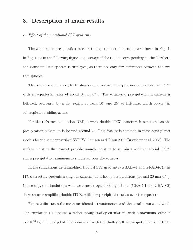
The reference simulation, REF, shows rather realistic precipitation values over the ITCZ,
with an equatorial value of about 8 mm d−1. The equatorial precipitation maximum is
followed, poleward, by a dry region between 10◦ and 25◦ of latitudes, which covers the
subtropical subsiding zones.
For the reference simulation REF, a weak double ITCZ structure is simulated as the
precipitation maximum is located around 4◦. This feature is common in most aqua-planet
models for the same prescribed SST (Williamson and Olson 2003; Brayshaw et al. 2008). The
surface moisture flux cannot provide enough moisture to sustain a wide equatorial ITCZ,
and a precipitation minimum is simulated over the equator.
In the simulations with amplified tropical SST gradients (GRAD+1 and GRAD+2), the
ITCZ structure presents a single maximum, with heavy precipitations (14 and 20 mm d−1).
Conversely, the simulations with weakened tropical SST gradients (GRAD-1 and GRAD-2)
show an over-amplified double ITCZ, with low precipitation rates over the equator.
Figure 2 illustrates the mean meridional streamfunction and the zonal-mean zonal wind.
The simulation REF shows a rather strong Hadley circulation, with a maximum value of
17×1010 kg s−1. The jet stream associated with the Hadley cell is also quite intense in REF,
8

with a jet core of about 60 m s−1.
The simulations with strong meridional SST gradients (GRAD+1 and GRAD+2) all
show a stronger Hadley circulation, with an intense jet stream. On the other hand, the
simulations with weak meridional SST gradients (GRAD-1 and GRAD-2) have a weaker
meridional streamfunction, whose maximum is far from the equator, at 25◦ for GRAD-2. In
GRAD-2, the jet stream is located at 50◦, far away from the Hadley cell. Furthermore, a
zone without any significant zonal-mean circulation is observed at the center of the double
ITCZ. In the following sections, we demonstrate that in the center of the double ITCZ, the
radiative-convective equilibrium prevails, and no large-scale organization of the flow occurs.
The Hadley cell and jet stream are characterized by their strength and their latitudinal
extent. The latitudinal extent of the Hadley cell is calculated as the latitude of the zero-value
streamfunction, linearly interpolated, and averaged between 700-hPa and 300-hPa. The
position of the jets is calculated as the latitude of the maximum zonal-mean zonal wind.
The Hadley cell strength is given by the maximum absolute value of the streamfunction,
averaged between the 700-hPa and 300-hPa heights, while the jet stream intensity is given
by the maximum zonal-mean zonal wind. The results are illustrated in Fig. 3.
The Hadley cell is clearly stronger when the tropical SST gradient is increased, although
the intensification with increased tropical gradient is much smaller than the weakening with
decreased tropical gradient. The expansion of the Hadley cell is closely correlated to its
strength. Indeed, the stronger the cell is, the narrower it is. A similar relation between
strength and extent of the Hadley cell was observed in ocean-atmosphere coupled models by
Lu et al. (2008). The jet stream intensity and position roughly correspond to those of the
Hadley cell. Nevertheless, we illustrate in the next section that the strong SST gradients
9
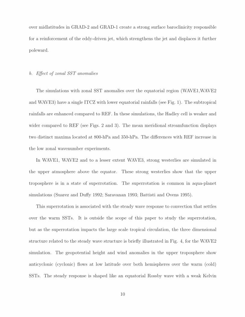
over midlatitudes in GRAD-2 and GRAD-1 create a strong surface baroclinicity responsible
for a reinforcement of the eddy-driven jet, which strengthens the jet and displaces it further
poleward.
b. Effect of zonal SST anomalies
The simulations with zonal SST anomalies over the equatorial region (WAVE1,WAVE2
and WAVE3) have a single ITCZ with lower equatorial rainfalls (see Fig. 1). The subtropical
rainfalls are enhanced compared to REF. In these simulations, the Hadley cell is weaker and
wider compared to REF (see Figs. 2 and 3). The mean meridional streamfunction displays
two distinct maxima located at 800-hPa and 350-hPa. The differences with REF increase in
the low zonal wavenumber experiments.
In WAVE1, WAVE2 and to a lesser extent WAVE3, strong westerlies are simulated in
the upper atmosphere above the equator. These strong westerlies show that the upper
troposphere is in a state of superrotation. The superrotation is common in aqua-planet
simulations (Suarez and Duffy 1992; Saravanan 1993; Battisti and Ovens 1995).
This superrotation is associated with the steady wave response to convection that settles
over the warm SSTs. It is outside the scope of this paper to study the superrotation,
but as the superrotation impacts the large scale tropical circulation, the three dimensional
structure related to the steady wave structure is briefly illustrated in Fig. 4, for the WAVE2
simulation. The geopotential height and wind anomalies in the upper troposphere show
anticyclonic (cyclonic) flows at low latitude over both hemispheres over the warm (cold)
SSTs. The steady response is shaped like an equatorial Rossby wave with a weak Kelvin
10
wave component. The momentum flux by stationary eddies is oriented equatorward, thus
transporting momentum from the midlatitudes to the equator, which contributes to the
superrotation. The Hadley cell intensifies in the upper levels to compensate for the strong
momentum flux by stationary eddies, which causes the upper-level maximum of the mean
meridional streamfunction, between 400-hPa and 300-hPa, in Fig. 2.
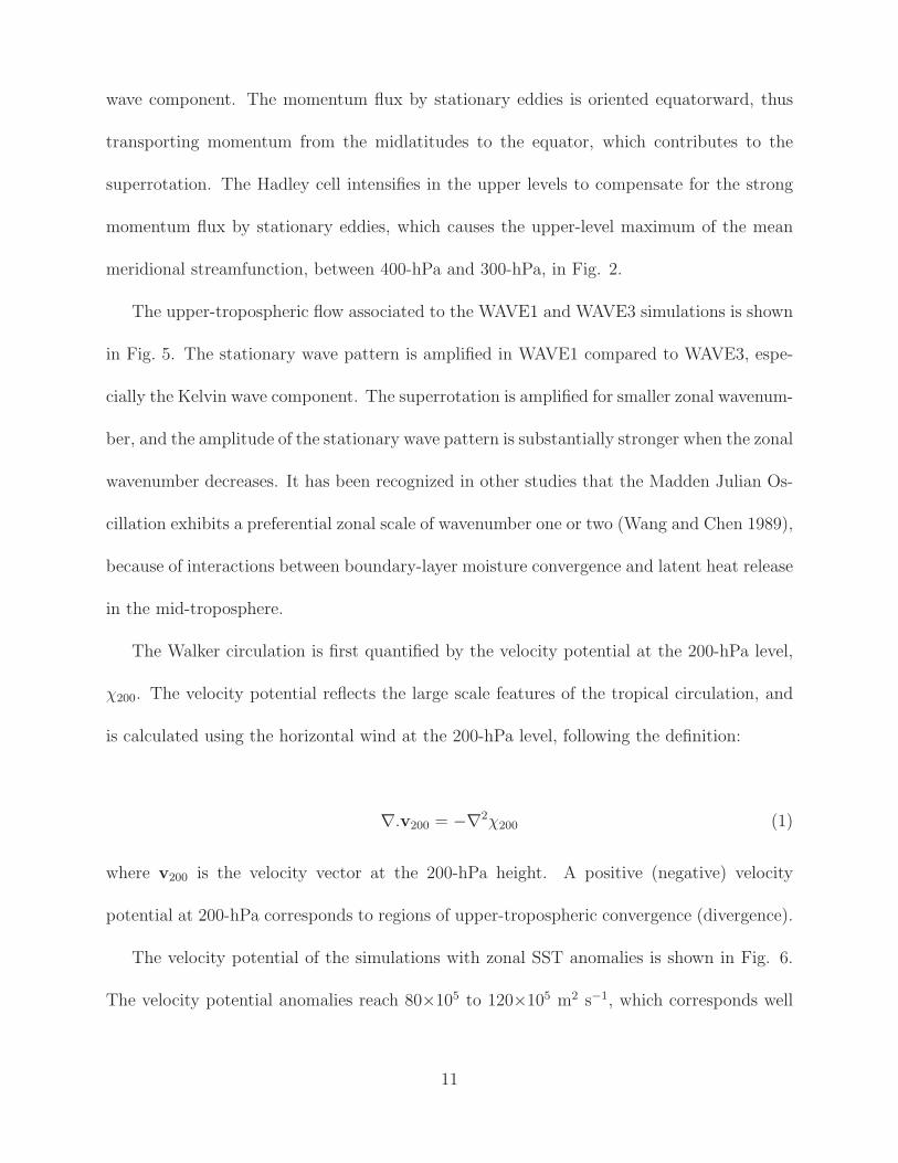
The upper-tropospheric flow associated to the WAVE1 and WAVE3 simulations is shown
in Fig. 5. The stationary wave pattern is amplified in WAVE1 compared to WAVE3, espe-
cially the Kelvin wave component. The superrotation is amplified for smaller zonal wavenum-
ber, and the amplitude of the stationary wave pattern is substantially stronger when the zonal
wavenumber decreases. It has been recognized in other studies that the Madden Julian Os-
cillation exhibits a preferential zonal scale of wavenumber one or two (Wang and Chen 1989),
because of interactions between boundary-layer moisture convergence and latent heat release
in the mid-troposphere.
The Walker circulation is first quantified by the velocity potential at the 200-hPa level,
χ200. The velocity potential reflects the large scale features of the tropical circulation, and
is calculated using the horizontal wind at the 200-hPa level, following the definition:
∇.v200 = −∇2χ200 (1)
where v200 is the velocity vector at the 200-hPa height. A positive (negative) velocity
potential at 200-hPa corresponds to regions of upper-tropospheric convergence (divergence).
The velocity potential of the simulations with zonal SST anomalies is shown in Fig. 6.
The velocity potential anomalies reach 80×105 to 120×105 m2 s−1, which corresponds well
11

to the values found in reanalysis (Tanaka et al. 2004). In the WAVE simulations, the regions
of upper-tropospheric divergence are located in the deep tropics, between 15◦N and 15◦S,
over the warm SST regions. Regions of convergence develop in both hemispheres, between
20◦ and 40◦, to the west of the main equatorial updrafts, as expected from the Gill model
response to a prescribed heating (Gill 1980). The upper-tropospheric circulation above the
equator, between 25◦N and 25◦S, is stronger when the zonal wavenumber increases.
The Walker circulation mass-flux is also calculated, to allow comparison with the merid-
ional streamfunction that conventionally measures the Hadley cell strength. A mass-flux can
be calculated within the domain of the Hadley circulation, since the zonal-mean mass flux is
zero at the meridional boundaries of the Hadley cell. In this paper, the extent of the Hadley
cells is computed on a monthly basis, in both the Northern and Southern Hemispheres, as
the latitude of the zero-value mean meridional streamfunction, averaged between 700-hPa
and 300-hPa. Then, a monthly zonal streamfunction is retrieved. The zonal streamfunction
is strongly sensitive to the vertical shear of the mean zonal wind, characterized by easter-
lies at lower levels and westerlies at upper levels in the tropics. The zonal streamfunction
circulation is also sensitive to the superrotation. Instead, we use the zonal anomalies of the
zonal mean streamfunction, ψ∗
x, which provide a better diagnostic of the Walker circulation
(see Appendix A).
Figure 7 shows the zonal streamfunction anomalies, ψ∗
x, in the domain of the Hadley
cells. The Walker circulation is the strongest for WAVE1, where the maximum streamfunc-
tion, averaged between the 700-hPa and 300-hPa heights, is 9.8×10¹⁰ kg s−1. If the zonal
wavenumber increases, the Walker circulation intensity decreases, while the Hadley circula-
tion intensity increases (see Fig. 3). The situation on Earth is similar to WAVE1, as only
12
two main cells are observed, even if the intensity is more similar to that of WAVE2 (see
Appendix A).
c. Effect of uniform SST warming
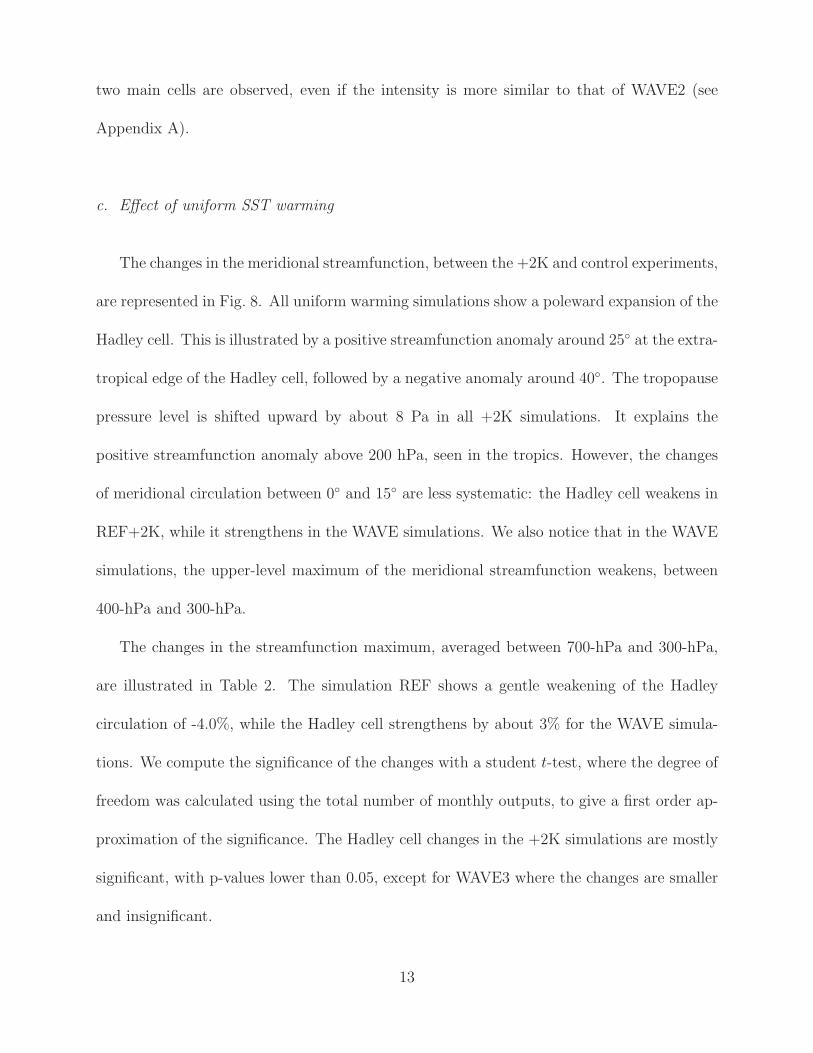
The changes in the meridional streamfunction, between the +2K and control experiments,
are represented in Fig. 8. All uniform warming simulations show a poleward expansion of the
Hadley cell. This is illustrated by a positive streamfunction anomaly around 25◦ at the extra-
tropical edge of the Hadley cell, followed by a negative anomaly around 40◦. The tropopause
pressure level is shifted upward by about 8 Pa in all +2K simulations. It explains the
positive streamfunction anomaly above 200 hPa, seen in the tropics. However, the changes
of meridional circulation between 0◦ and 15◦ are less systematic: the Hadley cell weakens in
REF+2K, while it strengthens in the WAVE simulations. We also notice that in the WAVE
simulations, the upper-level maximum of the meridional streamfunction weakens, between
400-hPa and 300-hPa.
The changes in the streamfunction maximum, averaged between 700-hPa and 300-hPa,
are illustrated in Table 2. The simulation REF shows a gentle weakening of the Hadley
circulation of -4.0%, while the Hadley cell strengthens by about 3% for the WAVE simula-
tions. We compute the significance of the changes with a student t-test, where the degree of
freedom was calculated using the total number of monthly outputs, to give a first order ap-
proximation of the significance. The Hadley cell changes in the +2K simulations are mostly
significant, with p-values lower than 0.05, except for WAVE3 where the changes are smaller
and insignificant.
13
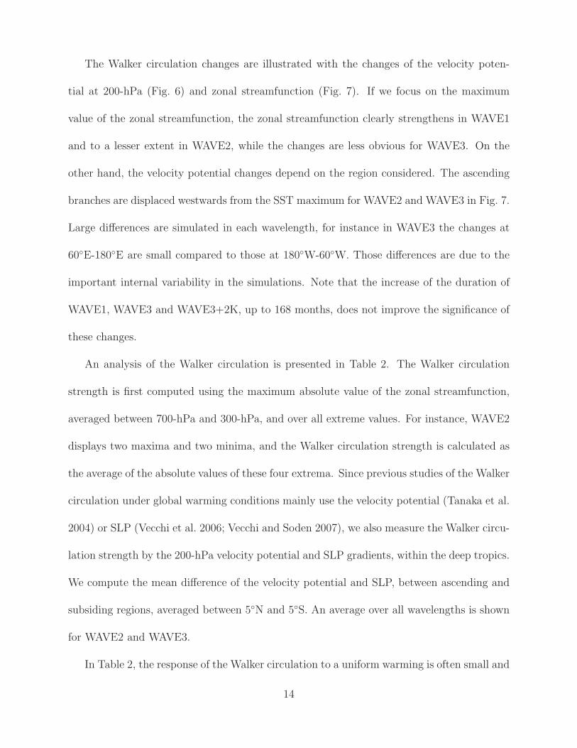
The Walker circulation changes are illustrated with the changes of the velocity poten-
tial at 200-hPa (Fig. 6) and zonal streamfunction (Fig. 7). If we focus on the maximum
value of the zonal streamfunction, the zonal streamfunction clearly strengthens in WAVE1
and to a lesser extent in WAVE2, while the changes are less obvious for WAVE3. On the
other hand, the velocity potential changes depend on the region considered. The ascending
branches are displaced westwards from the SST maximum for WAVE2 and WAVE3 in Fig. 7.
Large differences are simulated in each wavelength, for instance in WAVE3 the changes at
60◦E-180◦E are small compared to those at 180◦W-60◦W. Those differences are due to the
important internal variability in the simulations. Note that the increase of the duration of
WAVE1, WAVE3 and WAVE3+2K, up to 168 months, does not improve the significance of
these changes.
An analysis of the Walker circulation is presented in Table 2. The Walker circulation
strength is first computed using the maximum absolute value of the zonal streamfunction,
averaged between 700-hPa and 300-hPa, and over all extreme values. For instance, WAVE2
displays two maxima and two minima, and the Walker circulation strength is calculated as
the average of the absolute values of these four extrema. Since previous studies of the Walker
circulation under global warming conditions mainly use the velocity potential (Tanaka et al.
2004) or SLP (Vecchi et al. 2006; Vecchi and Soden 2007), we also measure the Walker circu-
lation strength by the 200-hPa velocity potential and SLP gradients, within the deep tropics.
We compute the mean difference of the velocity potential and SLP, between ascending and
subsiding regions, averaged between 5◦N and 5◦S. An average over all wavelengths is shown
for WAVE2 and WAVE3.
In Table 2, the response of the Walker circulation to a uniform warming is often small and
14
weakly significant. The zonal streamfunction increases in WAVE1, without any significant
changes of velocity potentials or SLP gradients. WAVE2+2K shows a weakly significant in-
tensification of the zonal streamfunction and a decrease in the equatorial velocity potentials,
while in WAVE3+2K only the equatorial SLP gradient decreases. The zonal streamfunction
represents the zonal circulation over the whole tropics, while the velocity potential and the
SLP gradients, averaged between 5◦N and 5◦S, represent the circulation in the deep tropics.
As the circulation changes in response to a uniform SST warming depend on the region
considered, these diagnostics give different results. The response also varies depending on
the zonal-wavenumber. For example, the Walker cells strengthen in WAVE1, while WAVE3
shows a weakening. In our simulations, the Walker circulation changes induced by a uni-
form SST warming are clearly small compared to the important weakening seen in models
or observations, where both the velocity potential and SLP gradient decrease (Tanaka et al.
2004; Vecchi et al. 2006; Vecchi and Soden 2007).
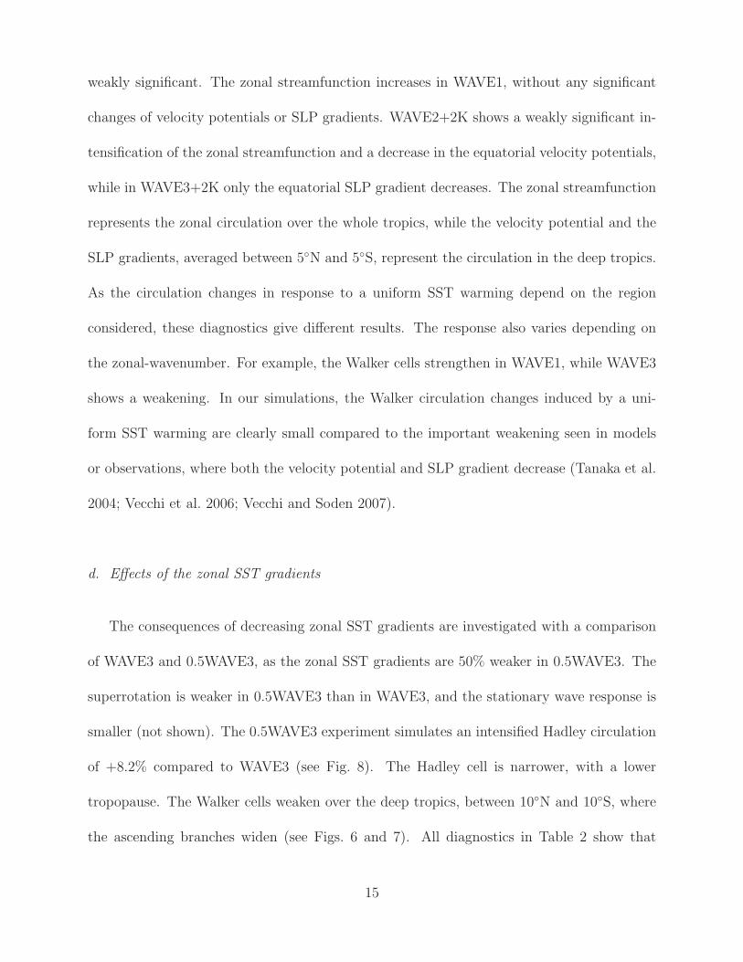
d. Effects of the zonal SST gradients
The consequences of decreasing zonal SST gradients are investigated with a comparison
of WAVE3 and 0.5WAVE3, as the zonal SST gradients are 50% weaker in 0.5WAVE3. The
superrotation is weaker in 0.5WAVE3 than in WAVE3, and the stationary wave response is
smaller (not shown). The 0.5WAVE3 experiment simulates an intensified Hadley circulation
of +8.2% compared to WAVE3 (see Fig. 8). The Hadley cell is narrower, with a lower
tropopause. The Walker cells weaken over the deep tropics, between 10◦N and 10◦S, where
the ascending branches widen (see Figs. 6 and 7). All diagnostics in Table 2 show that
15

the Walker cells weaken compared to WAVE3, the zonal streamfunction decreases by -8.8%,
and the velocity potential gradient decreases by -15.0%. The zonal SLP gradients are 50%
smaller, as expected from the 50% reduction of the SST anomalies (Lindzen and Nigam
1987).
These changes correspond well to the changes of the Hadley and Walker circulation
induced by ENSO. During El Nino (La Nina) events, warm (cold) SST anomalies in the
Central and Eastern Pacific Ocean decrease (increase) the zonal SST gradients, which results
in a weakening (strengthening) of the Walker cells and a strengthening (weakening) of the
Hadley cell (Oort and Yienger 1996). Surprisingly, the changes induced by a modification
of the zonal SST gradient are stronger and more significant than those simulated by a
uniform SST warming (see Table 2). Therefore, the modifications of the zonal SST gradient
in simulations with complete ocean-atmosphere coupled models could play a major role in
explaining the changes of the Hadley and Walker cells.
e. Thermodynamical state of the tropical atmosphere
Our simulations give a large variety of dynamic and thermodynamic states in the tropical
troposphere. Figure 9 depicts the mean tropical thermodynamic state of the tropical tropo-
sphere in our experiments, with the dry static stability at 500-hPa, Sp500, the precipitation,
P, the column integrated water vapor, W, and the 500-hPa mean ascending velocities, M+
500.
The dry static stability Sp500 is equivalent to the Brunt Vaisala frequency, and is defined as:
Sp = −T
θ
∂θ
∂p
16
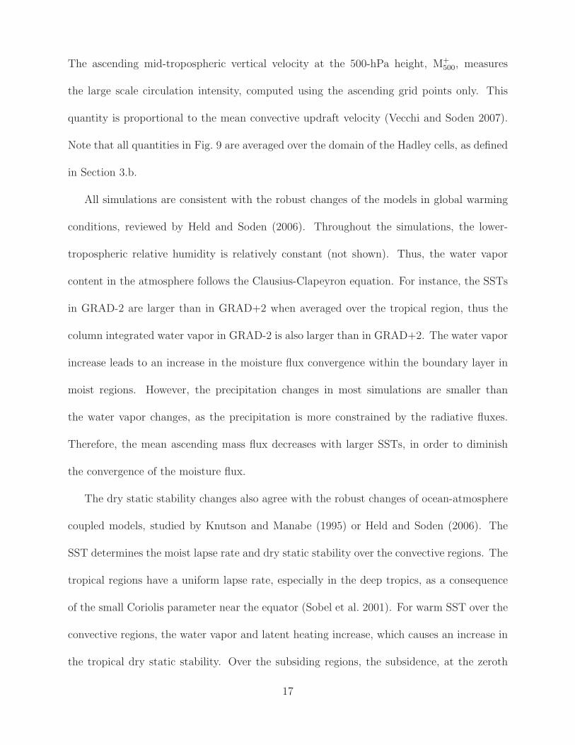
The ascending mid-tropospheric vertical velocity at the 500-hPa height, M+
500, measures
the large scale circulation intensity, computed using the ascending grid points only. This
quantity is proportional to the mean convective updraft velocity (Vecchi and Soden 2007).
Note that all quantities in Fig. 9 are averaged over the domain of the Hadley cells, as defined
in Section 3.b.
All simulations are consistent with the robust changes of the models in global warming
conditions, reviewed by Held and Soden (2006). Throughout the simulations, the lower-
tropospheric relative humidity is relatively constant (not shown). Thus, the water vapor
content in the atmosphere follows the Clausius-Clapeyron equation. For instance, the SSTs
in GRAD-2 are larger than in GRAD+2 when averaged over the tropical region, thus the
column integrated water vapor in GRAD-2 is also larger than in GRAD+2. The water vapor
increase leads to an increase in the moisture flux convergence within the boundary layer in
moist regions. However, the precipitation changes in most simulations are smaller than
the water vapor changes, as the precipitation is more constrained by the radiative fluxes.
Therefore, the mean ascending mass flux decreases with larger SSTs, in order to diminish
the convergence of the moisture flux.
The dry static stability changes also agree with the robust changes of ocean-atmosphere
coupled models, studied by Knutson and Manabe (1995) or Held and Soden (2006). The
SST determines the moist lapse rate and dry static stability over the convective regions. The
tropical regions have a uniform lapse rate, especially in the deep tropics, as a consequence
of the small Coriolis parameter near the equator (Sobel et al. 2001). For warm SST over the
convective regions, the water vapor and latent heating increase, which causes an increase in
the tropical dry static stability. Over the subsiding regions, the subsidence, at the zeroth
17

order, is given by the ratio between the atmospheric radiative cooling and the dry static
stability. The increase in dry static stability is accompanied by a smaller increase in radiative
cooling (not shown), which leads to a weakening the tropical circulation.
However, these mechanisms do not apply for all simulations. For instance, WAVE3
shows a stronger dry static stability compared to REF, but the mean ascending velocities
are stronger than REF. The changes of the mean ascending velocity are unable to quantify
the large scale organization of the flow. It has been recognized that a widening of the
area covered by ascending motions could induce a stronger circulation without modifications
of the mean ascending velocity (Pierrehumbert 1995). Furthermore, the Hadley cells are
expected to be governed by the SST meridional gradients (Held and Hou 1980; Gastineau
et al. 2009). To further understand the changes of the large scale circulation, one needs to
analyze the momentum and MSE budgets.
4. Mean zonal wind balance
The zonal-mean zonal wind shows a large variety of behaviors in our experiments. For
instance, the simulations using a zonal SST anomaly present a superrotation in the upper
tropical atmosphere. Another interesting phenomenon is observed in the simulations with a
weak tropical meridional SST gradient, where the maximum zonal wind is shifted poleward
with respect to the position of the Hadley cells. These singular behaviors can be explained
by the zonal momentum balance.
The terms of the zonal-mean zonal momentum equation are calculated following the
methodology used in Seager et al. (2003):
18
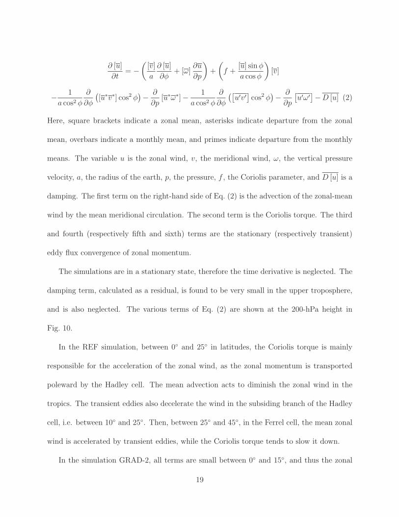
∂ [u]
∂t= −
(
[v]
a
∂ [u]
∂φ+ [ω]
∂u
∂p
)
+
(
f +[u] sin φ
a cos φ
)
[v]
−1
a cos2 φ
∂
∂φ
(
[u∗v∗] cos2 φ)
−∂
∂p[u∗ω∗]−
1
a cos2 φ
∂
∂φ
([
u′v′
]
cos2 φ)
−∂
∂p
[
u′ω′
]
−D [u] (2)
Here, square brackets indicate a zonal mean, asterisks indicate departure from the zonal
mean, overbars indicate a monthly mean, and primes indicate departure from the monthly
means. The variable u is the zonal wind, v, the meridional wind, ω, the vertical pressure
velocity, a, the radius of the earth, p, the pressure, f , the Coriolis parameter, and D [u] is a
damping. The first term on the right-hand side of Eq. (2) is the advection of the zonal-mean
wind by the mean meridional circulation. The second term is the Coriolis torque. The third
and fourth (respectively fifth and sixth) terms are the stationary (respectively transient)
eddy flux convergence of zonal momentum.
The simulations are in a stationary state, therefore the time derivative is neglected. The
damping term, calculated as a residual, is found to be very small in the upper troposphere,
and is also neglected. The various terms of Eq. (2) are shown at the 200-hPa height in
Fig. 10.
In the REF simulation, between 0◦ and 25◦ in latitudes, the Coriolis torque is mainly
responsible for the acceleration of the zonal wind, as the zonal momentum is transported
poleward by the Hadley cell. The mean advection acts to diminish the zonal wind in the
tropics. The transient eddies also decelerate the wind in the subsiding branch of the Hadley
cell, i.e. between 10◦ and 25◦. Then, between 25◦ and 45◦, in the Ferrel cell, the mean zonal
wind is accelerated by transient eddies, while the Coriolis torque tends to slow it down.
In the simulation GRAD-2, all terms are small between 0◦ and 15◦, and thus the zonal
19
wind is weak in the equatorial region. Between 15◦ and 30◦, the Coriolis and mean advection
terms are smaller compared to REF as the mean meridional circulation is weaker. The tran-
sient eddy momentum divergence is of a similar magnitude, but shifted polewards, between
10◦ and 30◦. This term becomes much stronger in the midlatitudes, between 30◦ and 70◦.
This is related to the very strong midlatitude SST gradients, which increases the baroclinicity
and the transport of momentum by transient eddies. These transient eddies give momentum
to the zonal-mean zonal wind, which enhances the eddy-driven jet. A similar effect was
obtained by Brayshaw et al. (2008) when the midlatitude SST gradients were specifically
modified. The subtropical jet, that is more dependent on the momentum divergence by the
mean meridional circulation, is decreased, as the Hadley cell is weak.
In WAVE3, the stationary wave pattern is clearly responsible for a convergence of mo-
mentum in the equatorial region, between 0◦ and 5◦, where it causes the superrotation,
as shown in Section 3.b. Elsewhere, the stationary eddy momentum flux is smaller than
the other terms. The Coriolis and mean advection terms are smaller in WAVE3, as the
Hadley cell is weaker. An analysis of WAVE1 or WAVE2 gives qualitatively similar results.
The modifications of the zonal wind in WAVE3 are small beyond 30◦, and the maximum
zonal-mean zonal-wind is almost unchanged despite a large weakening of the Hadley cell.
The changes affecting the zonal-mean wind in our simulations correspond well to those
of the transient and stationary eddies that displace and amplify the eddy-driven jets. The
intensity of the Hadley cell is associated to the Coriolis torque and mean momentum advec-
tion terms. The locations of the maximum momentum flux convergence by the zonal-mean
circulation and eddies are computed to illustrate the positions of the subtropical, φSTJ ,and
eddy-driven, φEDD, jets.
20

φSTJ where1
a cos φ
∂[u][v] cos φ
∂φis maximum (3)
φEDD where1
a cos φ
∂([u′v′] + [u∗v∗]) cos φ
∂φis maximum (4)
These positions are added in Fig. 3. The eddy-driven jet is clearly responsible for the
poleward displacement of the maximum zonal wind in GRAD-1 and GRAD-2, but also in
the +2K simulations. In the +2K simulations, the Hadley cell expansion is analogous to
that of ocean-atmosphere coupled models in global warming conditions (Lu et al. 2007).
This extension is governed in these models by the increase of the dry static stability which
prevents the penetration of midlatitude eddies into the tropics (Lu et al. 2008).
5. Budgets of moist static energy
In this section, the large-scale tropical circulation is analyzed through the moist static
energy (MSE) variable. The MSE quantifies the energy transported by air parcels and is
defined as m = s + Lvq, where s = CpT + gz is the DSE (Dry Static Energy) and Lvq is the
latent heat.
The column-average MSE budget is :
∇.(vm) = QR + H + LvE, (5)
where v is the wind vector. The overbars designate monthly and vertical averaging. H the
turbulent sensible heat flux, E the turbulent evaporation flux. QR is the net atmospheric
radiative heating rate, diagnosed from the budget of the radiative flux at the surface and
21
top of the atmosphere.
a. Meridional transports of moist static energy
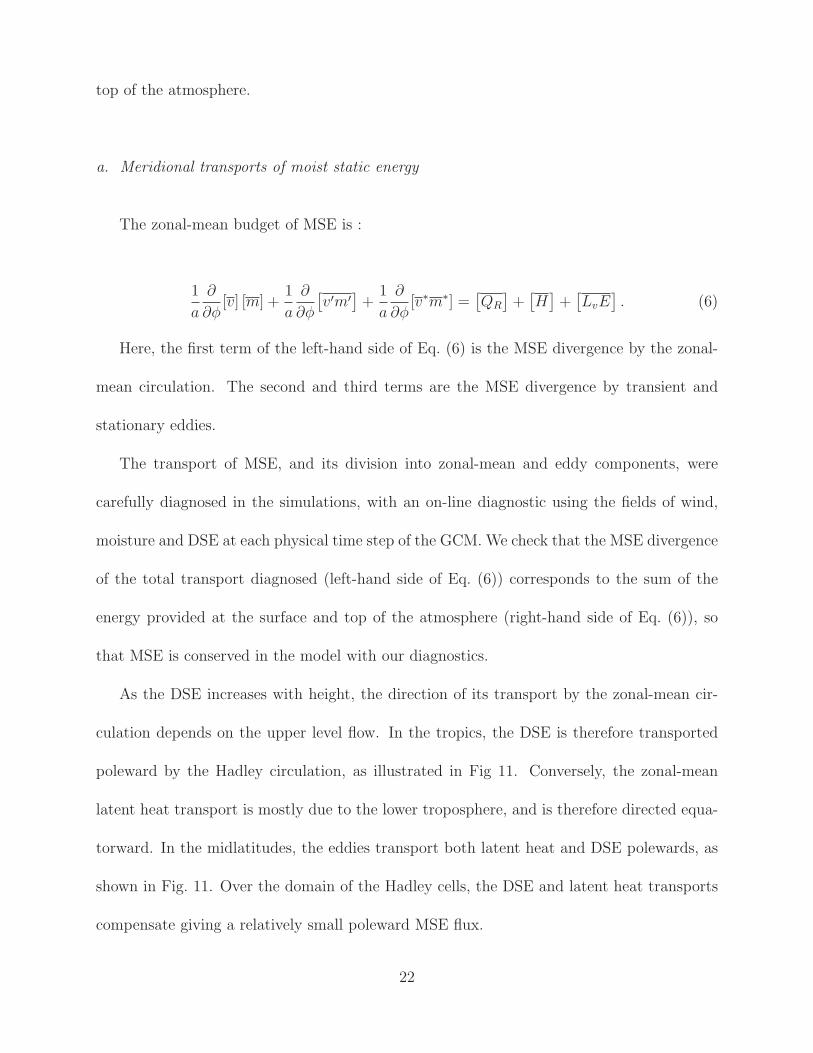
The zonal-mean budget of MSE is :
1
a
∂
∂φ[v] [m] +
1
a
∂
∂φ
[
v′m′
]
+1
a
∂
∂φ[v∗m∗] =
[
QR
]
+[
H]
+[
LvE]
. (6)
Here, the first term of the left-hand side of Eq. (6) is the MSE divergence by the zonal-
mean circulation. The second and third terms are the MSE divergence by transient and
stationary eddies.
The transport of MSE, and its division into zonal-mean and eddy components, were
carefully diagnosed in the simulations, with an on-line diagnostic using the fields of wind,
moisture and DSE at each physical time step of the GCM. We check that the MSE divergence
of the total transport diagnosed (left-hand side of Eq. (6)) corresponds to the sum of the
energy provided at the surface and top of the atmosphere (right-hand side of Eq. (6)), so
that MSE is conserved in the model with our diagnostics.
As the DSE increases with height, the direction of its transport by the zonal-mean cir-
culation depends on the upper level flow. In the tropics, the DSE is therefore transported
poleward by the Hadley circulation, as illustrated in Fig 11. Conversely, the zonal-mean
latent heat transport is mostly due to the lower troposphere, and is therefore directed equa-
torward. In the midlatitudes, the eddies transport both latent heat and DSE polewards, as
shown in Fig. 11. Over the domain of the Hadley cells, the DSE and latent heat transports
compensate giving a relatively small poleward MSE flux.
22
The MSE fluxes, and their decomposition into mean, stationary and transient components
are given in Fig. 12. All simulations have a maximum energy flux located between 35◦ and
40◦, with a similar intensity. GRAD+2 (GRAD-2) shows an amplified (reduced) poleward
energy flux in the tropics. The differences among the total MSE flux of the simulations REF,
REF+2 and WAVE are smaller.
The MSE budget is further illustrated in Fig. 13, by the different terms at the right-hand
side of Eq. (6). In REF, between the equator and 35◦, the evaporation and, to a lesser
extent, sensible heating, provide MSE to the atmosphere, while the radiative cooling emits
a smaller part of that energy towards space. The MSE fluxes are divergent. Beyond 35◦,
the loss of energy due to radiative cooling is the dominant term, and the MSE fluxes are
convergent.
In GRAD+2, between 0◦ and 5◦, the evaporation provides a large amount of energy at the
surface while the radiative cooling is not strong enough to compensate. A vigorous Hadley
circulation transports a large amount of MSE toward the poles. Conversely, between 5◦ and
40◦, the latent heat flux is smaller than in REF and the exported MSE from this region
decreases. In GRAD+2, this evaporation increase could be explained by the Wind-Induced
Surface Heat Exchange (WISHE) that may act as a positive feedback and strengthen the
large-scale circulation (Numaguti 1993, 1995; Boos and Emanuel 2008). However, another
set of simulations with prescribed surface fluxes needs to be performed to properly document
the role of WISHE.
In GRAD-2, between 0◦ and 10◦, the MSE provided by the turbulent fluxes is nearly equal
to the radiative cooling. Therefore, the Hadley circulation is negligible and the radiative-
convective equilibrium prevails. However, between 15◦ and 30◦, the evaporation is strong and
23
the MSE flux strengthens. The transient eddy MSE flux mainly accounts for this stronger
MSE flux.
In the WAVE3 or REF+2K simulations, more energy is provided by the turbulent fluxes
at the surface. For REF+2K the turbulent fluxes are stronger everywhere, while for WAVE3,
the changes are confined to the equatorial region. In both simulations, a stronger radiative
cooling occurs at the same latitudes, and the energy excess is radiated to space. Therefore,
the MSE fluxes are only weakly modified in these simulations.
b. Zonal transport of Moist Static Energy
The MSE budget (Eq. (6)) is averaged over the domain of the Hadley cells :
〈∇.(vm)〉 = 〈QR〉 + 〈H〉 + 〈LvE〉 (7)
where angle brackets indicate the average over the domain of the Hadley cells (see Section
3.b). Here, the term on the left-hand side describes the total MSE divergence, due to the
Walker and Hadley circulations (i.e. 〈∇.(v m)〉) and transient eddies (i.e. 〈∇.(v′m′)〉). The
right-hand side terms describe the energy provided in the Hadley cells domain by radiative
cooling, sensible and latent heat fluxes.
The zonal anomalies of the terms on the right-hand side of Eq. (7) are shown in Fig. 14,
for the simulations WAVE1, WAVE1+2K, WAVE3, WAVE3+2K and 0.5WAVE3. Over
the cold (warm) SST anomalies, the radiative cooling and turbulent fluxes present large
negative (positive) anomalies. As a consequence, the Walker circulation transports MSE
directly from the warm SST regions to the cold ones. The zonal anomalies of the mean
24
meridional circulation and eddies also contribute to this MSE transport.
In WAVE1+2K, the zonal gradient of latent heat flux increases as a response to the SST
warming. The increase of the latent heat flux is mainly due to the exponential dependence of
the saturation water vapor pressure on temperature, following the Clausius-Clapeyron rela-
tionship. The increase of evaporation is stronger over the warm SST regions. The large-scale
atmospheric circulation transports more MSE and the Walker circulation strengthens. On
the other hand, in WAVE3+2K, the increase in turbulent flux anomalies is less systematic,
and the turbulent heat fluxes decrease over the warm SSTs located at 50◦E or 150◦E. These
changes are associated with a gentle weakening of the Walker cells (see Table 2). The evap-
oration anomalies also decrease (increase) over the eastern (western) edge of the warm SST
anomalies, which contributes to a westward shift of the ascending zones in Fig. 6. It can
be concluded that the Walker cells intensity corresponds to the zonal gradient of turbulent
heat flux. For a uniform SST warming, the changes of the turbulent heat flux depends on
the pattern of the control SST.
In 0.5WAVE3, the anomalies between warm and cold regions are strongly reduced when
compared to WAVE3. As the amplitude of the SST anomalies are reduced, the turbulent
fluxes and radiative cooling anomalies are also smaller. The large-scale circulation transports
less MSE from the warm regions to the cold ones. Therefore, the Walker cells weaken when
the zonal SST gradients are reduced.
25

c. Role of moist static stability
The links between the MSE flux and the Hadley cell are complex. The mean meridional
circulation transports an important part of the total MSE flux in the tropics, while eddies
dominate in higher latitudes (see Fig. 12). In the tropics, the MSE transport is determined
by the compensation between the DSE and latent heat fluxes (see Fig. 11). The gross moist
static stability is commonly used to measure the ratio between the DSE and latent heat
fluxes, and quantifies the efficiency of the MSE transport by the mean meridional circulation
(Neelin and Held 1987). The gross moist static stability is associated with the geographical
distribution of convection. It is also linked to the convection scheme used (Frierson 2007).
The gross moist static stability, ∆m, is defined as the ratio between the zonal-mean MSE
flux and the intensity of the meridional circulation :
∆m =
∫
0
Ps[v][m]dp
∫ Pm
Ps[v]dp
(8)
where the overbars denote a time averaging. Ps is the surface pressure. Pm is a mid-
tropospheric level where the vertical velocity is maximum, commonly found around 500-hPa.
The unit of the gross moist static stability is kJ kg−1. It is the amount of MSE transported
per kg of mean meridional mass circulation. The denominator on the right-hand side of
Eq. (8) is the intensity of the meridional circulation. This formulation of the gross moist
static stability is similar to that of Neelin and Held (1987), but follows the definition of
Frierson et al. (2007) by defining it as a ratio of flux rather than flux divergence.
We define C, the ratio of the total MSE flux transported by the mean meridional circu-
lation.
26

C =
∫
0
Ps[v][m]dp
F(9)
where F is the total zonal-mean MSE flux, defined as∫
0
Ps[vm]dp. The ratio C quantifies the
contribution of zonal mean circulation in the total MSE flux. An increase of eddy MSE flux
for the same total MSE flux leads to a reduced ratio C. We find a simple relation, analogous
to Kang et al. (2009) to describe the intensity of the meridional circulation:
∫
0
Ps
[v]dp =CF
∆m(10)
The gross moist static stability, ∆m, of the simulations is shown in Fig. 15. Furthermore,
the gross moist static stability, ∆m, the ratio C, and the total MSE flux, F , are estimated
between 2.5◦ and 15◦, where the mean meridional streamfunction is the strongest. The
results are shown in Fig.16.
In the REF simulation, the poleward MSE flux is 1.1 PW. The Hadley cell is responsible
for 28% of the total MSE flux. The gross moist static stability is quite small, i.e. 3.0 kJ kg−1.
As the deep tropical SSTs are warm, atmospheric convection is frequent, which homogenizes
the MSE profiles (∆m ≈ 0).
In the amplified tropical SST gradient simulations (GRAD+1 and GRAD+2), the total
MSE flux increases, as the evaporation provided in the deep tropics increases (see Fig. 13),
which strengthens the Hadley cell. Nevertheless, the gross tropical moist static stability also
increases, as most of the convection is located over the equator, while the region between 5◦
and 25◦ experiences less convection than REF (see precipitation in Fig. 1). Therefore, the
Hadley cell intensity is only weakly enhanced.
27
In the reduced tropical gradient simulations (GRAD-2 and GRAD-1), the Hadley cells
are displaced into the midlatitudes. The total MSE flux is much lower than REF in the deep
tropics. The Hadley circulation is negligible in the deep tropics as the radiative-convective
equilibrium prevails over such weak SST gradient conditions (Held and Hou 1980). Note
that for the experiment GRAD-1, an inverse weak overturning cell appears in the deep
tropics, causing negative values of the gross moist static stability in Figs. 15 and 16. In
these simulations, the Hadley cells are located in the midlatitudes (around 25◦ for GRAD-
2), where the moist static stability is larger than in the deep tropics, which further weakens
the Hadley cells.
In the simulations with zonal SST anomalies (WAVE1, WAVE2, WAVE3 and 0.5WAVE3),
some subsiding motions occurs in the deep tropics, as convection is inhibited over the cold
SST regions (see Fig. 6). Therefore, the zonal-mean gross moist static stability increases over
the deep tropics compared to REF (see lower panel of Fig. 15). The total MSE flux increases
in these simulations (Fig. 16), but the increase in gross moist static stability is stronger, so
that the mean meridional circulation weakens. In the high zonal wavenumber simulations,
such as WAVE3, the zonal SST gradient is locally stronger than in the low wavenumber
cases (i.e. WAVE1), and the turbulent fluxes are enhanced by strong low-level winds. The
reinforcement of the total MSE flux may explain the strengthening of the Hadley cells when
the zonal wavenumber increases.
In the +2K simulations, the total MSE transport is almost invariant (see Figs. 12 and 15).
All simulations show a decrease of the deep tropical gross moist static stability. This decrease
is associated with the moistening of the lower troposphere, which exceeds the increase of dry
static stability in the upper troposphere. This effect is compensated by a decrease of C, the
28

fraction of the total MSE flux performed by the mean meridional circulation (see Fig. 16),
which corresponds to a reinforcement of the eddy component of the MSE flux. In REF, the
decrease of C prevails, while in the WAVE simulations, the changes of the gross moist static
stability are larger. We conclude that the Hadley circulation changes induced by a uniform
SST increase are highly dependent on the pattern of the control SST, as it determines the
changes resulting from the eddy MSE flux and gross moist static stability.
6. Discussion and conclusion
The parameters that determine the strength of the Hadley and Walker circulation in a
GCM are studied through various idealized aqua-planet simulations, using a GCM with a
comprehensive physical package. Four types of simulations are studied : (1) simulations with
axisymmetric SSTs where the meridional SST gradient is modified; (2) simulations with a
longitudinal equatorial wave-shaped SST anomaly; (3) uniform warming simulations of 2K;
(4) simulations where the equatorial zonal SST gradient is modified.
Drastic changes are seen when the meridional SST gradient is modified. A SST profile
with a maximum peaked at the equator produces a strong Hadley circulation, with a small
extent accompanied by a strong jet. For large tropical SST gradients, a vigorous Hadley cir-
culation is expected from the classical angular momentum framework. As convection settles
in the vicinity of the equator, the tropical gross moist static stability increases, which lessens
the Hadley cells intensification. Nevertheless, as our simulations use fixed SST conditions,
evaporation anomalies can increase without an accompanying SST decrease, and the Hadley
cell intensity may have been overestimated. This case of strong and narrow Hadley cell
29
shares some characteristics with the climate of the last glacial maximum (Williams 2006;
Broccoli et al. 2006).
In the case of a very flat SST distribution at the equator, a double ITCZ is simulated.
The Hadley cells are very weak with a large spatial extent. As the radiative-convective
equilibrium is possible, the classical angular momentum theory predicts that no large scale
organization of the flow occurs in the tropics (Held and Hou 1980). In this case, the Hadley
cells and MSE flux are governed by eddy dynamics. As very strong meridional SST gradients
are located in the midlatitudes, the midlatitude baroclinicity increases and the eddy-driven
jet is enhanced. It is likely that an analogous circulation existed during warm episodes of
past climate, such as the Eocene or the late Cretaceous, even if it is still unclear how such
SST gradients can be sustained by ocean-atmosphere coupling.
A significant weakening of the Hadley cell is induced by the introduction of the SST wave-
shaped anomaly. Such a configuration induces a superrotation in the upper-troposphere
and the formation of stationary eddies in the tropics. In addition, the gross moist static
stability increases, as convection is inhibited over the tropical subsiding zones. The poleward
MSE transport by the Hadley cells is more efficient, without any modifications of the total
MSE fluxes, and therefore the Hadley cells slow down. The superrotation is a caveat in
our simulations, as such a state is not observed in present-day climate. The presence of
superrotation may be due to the absence of cross equatorial SST gradient in perpetual
equinox conditions (Kraucunas and Hartmann 2005) and it would be interesting to repeat
our experiments in the case of the solstices. However, the mechanisms that weaken the
Hadley cells in the presence of longitudinal SST anomalies are still valid for present-day
climate.
30
A uniform warming of +2K induces non-systematic modifications of the Hadley and
Walker circulations, even if the mean updraft velocity diminishes in all simulations. A
uniform warming of +2K leads to a weakening of the Hadley cells in the reference simulation,
due to an enhancement of the MSE flux by transient eddies. With the introduction of a warm
pool and a cold SST region, the Hadley circulation increases in the case of a warming, due to
a decrease of moist static stability. Therefore, the Hadley circulation induced by a uniform
SST warming depends on the control SST pattern, which determines characteristics of the
transient and stationary eddy fluxes. On the other hand, the Walker circulation increases
(decreases) in the simulation with a zonal wavenumber 1 (3) and the reasons for these
different changes are still to be rigorously established. We suggest that the evaporation
anomalies are enhanced in our uniform warming simulations, which enhances the Walker
cells. In the case of a high zonal wavenumber, the Walker cells may also be affected by
changes in the transient and stationary eddy flux divergence of MSE.
The weakening of the zonal equatorial SST anomalies causes a weakening of the Walker
cells and a strengthening of the Hadley cells. The Hadley cells strengthen mainly because
the zonal-mean gross moist static stability diminishes, as the ascending branches are wider
and convection is more uniformly distributed over the tropics. The weakening of the Walker
cells corresponds well to the decrease of MSE provided by the anomalous turbulent fluxes in
the tropics.
Aqua-planet simulations represent simple intermediate-complexity tools suitable for study-
ing the atmospheric dynamics. Such simulations show a lot of deficiencies such as the double
ITCZ or superrotation. But the simplicity of these experiments also allows us to isolate a few
mechanisms that may have modified the tropical large-scale circulation in past- or future-
31
climate SSTs. Such processes are more difficult to detect in realistic situations because of
the complexity introduced by orography, land-ocean contrasts or non-linearities associated
with the seasonal cycle (Lindzen and Hou 1988).
In a global warming scenario, ocean-atmosphere coupled models, or models coupled to
an ocean mixed-layer, show a strong weakening of the Walker circulation (Vecchi and Soden
2007), while the Hadley cells only show a gentle decrease (Vecchi and Soden 2007; Gastineau
et al. 2008). In our simulations, such changes are not obtained with uniform SST warming.
How can we explain these differences? We suggest three explanations:
• Firstly, the fixed SST lower boundary conditions in our simulations could lead to
unrealistic values of the evaporation and cloud changes, as the SST is not allowed to
interact with the atmosphere. The surface turbulent flux and the clouds are expected
to be different in coupled ocean-atmosphere models, which can affect the Hadley and
Walker circulations.
• Secondly, the stationary and transient eddies are obviously unrealistic in our simula-
tions, due to the absence of continents and mountains, and the eddies through their
interactions with the diabatic and friction processes play a crucial role in driving the
Hadley cells (Kim and Lee 2001).
• Lastly, we also argue that the weaker Pacific Ocean zonal SST gradient simulated by
most ocean-atmosphere coupled models in global warming conditions may govern part
of the Walker circulation weakening. It may also explain the different changes of the
Hadley and Walker cells in ocean-atmosphere coupled models. When the zonal SST
gradient decreases, we find a weakening of the Walker cells and a strengthening of the
32
Hadley cells. Such an effect is analogous to that observed during El Nino events in
observations (Oort and Yienger 1996). However, the decrease of the SST gradient in
the Equatorial Pacific Ocean obtained in ocean-atmosphere coupled models (≈ 0.5◦K)
is relatively low compared to the applied 3◦K decrease of the SST gradient in our
simulations.
The tropical large scale circulation response simulated by the ocean-atmosphere cou-
pled models is not fully reproduced by our aqua-planet simulations, although they include
the water vapor and dry static stability changes. This is a clear demonstration that our
understanding of these circulations is not sufficient and requires more study.
Acknowledgments.
This work was supported by a PhD grant from the Universite Pierre et Marie Curie, Paris,
France. We thank Dargan M.W. Frierson, and two anonymous reviewers who contributed
to improve this manuscript.
33
APPENDIX A
The zonal streamfunction anomalies as a diagnostic of
the Walker cells
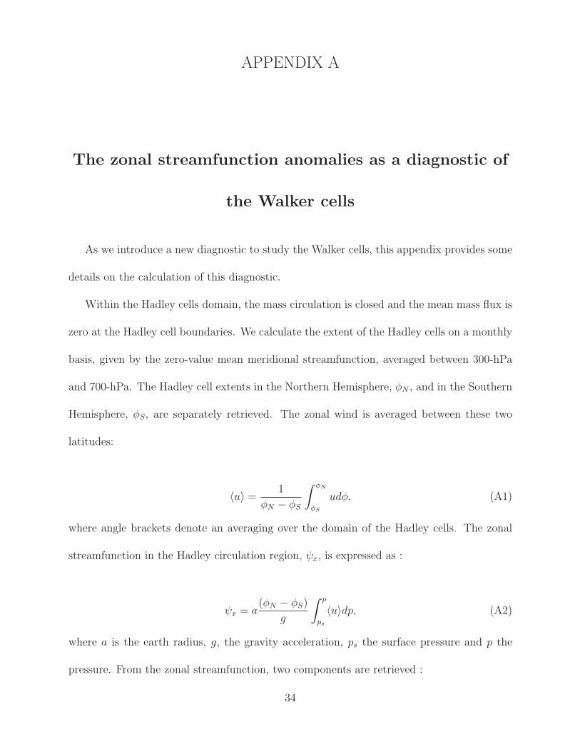
As we introduce a new diagnostic to study the Walker cells, this appendix provides some
details on the calculation of this diagnostic.
Within the Hadley cells domain, the mass circulation is closed and the mean mass flux is
zero at the Hadley cell boundaries. We calculate the extent of the Hadley cells on a monthly
basis, given by the zero-value mean meridional streamfunction, averaged between 300-hPa
and 700-hPa. The Hadley cell extents in the Northern Hemisphere, φN , and in the Southern
Hemisphere, φS, are separately retrieved. The zonal wind is averaged between these two
latitudes:
〈u〉 =1
φN − φS
∫ φN
φS
udφ, (A1)
where angle brackets denote an averaging over the domain of the Hadley cells. The zonal
streamfunction in the Hadley circulation region, ψx, is expressed as :
ψx = a(φN − φS)
g
∫ p
ps
〈u〉dp, (A2)
where a is the earth radius, g, the gravity acceleration, ps the surface pressure and p the
pressure. From the zonal streamfunction, two components are retrieved :
34

ψx = [ψx] + ψ∗
x (A3)
where square brackets indicate zonal averaging, and asterisks designate zonal anomalies.
[ψx] is proportional to the vertical shear of the zonal-mean zonal wind. The residual ψ∗
x
represents the Walker circulation . Figure 17 shows the zonal-mean zonal streamfunction,
[ψx], and the zonal streamfunction anomalies, ψ∗
x, from the ERA40 reanalysis (Uppala et al.
2005), during the 1979-2001 period.
Strong ascending motions are located over the western Pacific Ocean. Weaker and nar-
rower ascents are located over the eastern Pacific, Atlantic and Indian Ocean, therefore the
anomalous zonal circulation shows some subsiding motions over these regions.
Note that the use of an average between 25◦N and 25◦S, instead of an average over the
domain of the Hadley cells, provides similar results. So these results are not sensitive to the
precise definition of the latitudes used to delimit the Walker circulation.
35

REFERENCES
Battisti, D. S. and D. D. Ovens, 1995: The dependence of the low-level equatorial easterly
jet on Hadley and Walker circulations. J. Atmos. Sci., 52, 39113931.
Boos, W. R. and K. A. Emanuel, 2008: Wind-evaporation feedback and abrupt seasonal
transition of axisymmetric Hadley circulation. J. Atmos. Sci., 65, 2194–2214.
Brayshaw, D., B. Hoskins, and M. Blackburn, 2008: The storm-track response to idealized
SST perturbations in an aquaplanet GCM. J. Atmos. Sci., 65 (9), 2842–2860.
Broccoli, A. J., K. A. Dahl, and R. J. Stouffer, 2006: Response of the ITCZ to Northern
Hemisphere cooling. Geophys. Res. Lett., 33, L01 702, doi:10.1029/2005GL024 546.
Cess, R. D. and G. L. Potter, 1988: A methodology for understanding and intercomparing
atmospheric climate feedback processes in general circulation models. J. Geophys. Res.,
93, 8305–8314.
Di Nezio, P. N., A. Clement, G. Vecchi, B. Soden, B. Kirtman, and S.-K. Lee, 2009: Climate
Response of the Equatorial Pacific to Global Warming. J. Climate, 22, 4873–4892.
Emanuel, K. A., 1993: A cumulus representation based on the episodic mixing model: the
importance of mixing and microphysics in predicting humidity. AMS Meterol Monogr,
24 (46), 185–192.
36

Emanuel, K. A., J. D. Neelin, and C. S. Bretherton, 1994: On large-scale circulations in
convecting atmospheres. Q. J. R. Meteorol. Soc., 120 (519), 1111–1143.
Frierson, D. M. W., 2007: The dynamics of idealized convection schemes and their effect on
the zonally averaged tropical circulation. J. Atmos. Sci., 64, 1959–1976.
Frierson, D. M. W., 2008: Midlatitude static stability in simple and comprehensive general
circulation models. J. Atmos. Sci., 65, 1049–1062.
Frierson, D. M. W., I. M. Held, and P. Zurita-Gotor, 2007: A gray-radiation aquaplanet
moist GCM. Part II: energy transports in altered climates. J. Atmos. Sci., 64, 1680–1693.
Gastineau, G., H. L. Treut, and L. Li, 2008: Hadley circulation changes under global warming
conditions indicated by coupled climate models. Tellus A, 60 (5), 863–884.
Gastineau, G., H. L. Treut, and L. Li, 2009: The Hadley and Walker circulations changes
in global warming conditions described by idealized atmospheric simulations. J. Climate,
22, 3993–4013.
Gill, A. E., 1980: Some simple solutions for heat induced tropical circulations. Q. J. R. Me-
teorol. Soc., 106, 447–462.
Held, I. M. and A. Y. Hou, 1980: Nonlinear axially symmetric circulations in a nearly inviscid
atmosphere. J. Atmos. Sci., 37, 515–533.
Held, I. M. and B. J. Soden, 2006: Robust responses of the hydrological cycle to global
warming. J. Climate, 19, 5686–5699.
37
Hourdin, F., et al., 2006: The LMDZ4 general circulation model: climate performance and
sensitivity to parametrized physics with emphasis on tropical convection. Clim. Dyn., 27,
787–813.
Huber, M., 2009: Climate change: Snakes tell a torrid tale. Nature, 457, 669–671,
doi:10.1038/457 669a.
Kang, S. M., D. M. W. Frierson, and I. M. Held, 2009: The tropical response to extratrop-
ical forcing in an idealized GCM: the importance of radiative feedbacks and convective
parametrisation. J. Atmos. Sci., 66, 2812–2827.
Kim, H. K. and S. Y. Lee, 2001: Hadley cell dynamics in a primitive equation model. Part
II: Nonaxisymmertic flow. J. Atmos. Sci., 58, 2859–2871.
Knutson, T. and S. Manabe, 1995: Time mean response over the tropical pacific to increased
CO2 in a coupled ocean-atmosphere model. J. Climate, 8, 2181–2199.
Kraucunas, I. and D. Hartmann, 2005: Equatorial superrotation and the factors controlling
the zonal-mean zonal winds in the tropical upper troposphere. J. Atmos. Sci., 62, 371–389.
Kump, L. R. and D. Pollard, 2008: Amplification of cretaceous warmth by biological cloud
feedbacks. Science, 320 (5873), 195, doi:10.1126/science.1153 883.
Lindzen, R. S. and A. Y. Hou, 1988: Hadley circulations for zonally averaged heating centered
off the equator. J. Atmos. Sci., 45 (17), 2416–2427.
Lindzen, R. S. and S. Nigam, 1987: On the role of sea surface temperature gradients in
forcing low-level winds and convergence in the tropics. J. Atmos. Sci., 44, 2418–2436.
38
Lu, J., G. Chen, and D. M. W. Frierson, 2008: Response of the zonal mean atmospheric
circulation to El Nino versus global warming. J. Climate, 21, 5835–5851.
Lu, J., G. A. Vecchi, and T. Reichler, 2007: Expansion of the Hadley cell under global
warming. Geophys. Res. Lett., 34, L06 805, doi:10.1029/2006GL028 443.
Manabe, S., K. Bryan, and M. J. Spelman, 1975: A global ocean-atmosphere climate model.
Part I: The atmospheric circulation. J. Phys. Oceanogr., 5, 3–29.
Mitas, C. M. and A. Clement, 2005: Has the Hadley cell been strengthening in recent
decades? Geophys. Res. Lett., 32, L01 810, doi:10.1029/2005GL024 406.
Neale, R. B. and B. J. Hoskins, 2001a: A standard test for AGCMs including their physical
parametrizations: I: The proposal. Atmos. Sci. Lett., 1, doi:10.1006/asle.2000.0019.
Neale, R. B. and B. J. Hoskins, 2001b: A standard test for AGCMs including their
physical parametrizations: II: Results for the Met Office model. Atmos. Sci. Lett., 1,
doi:10.1006/asle.2000.0020.
Neelin, J. and I. M. Held, 1987: Modeling tropical convergence based on the moist static
energy budget. Mon. Wea. Rev., 115, 3–12.
Numaguti, A., 1993: Dynamics and energy balance of the hadley circulation and the trop-
ical precipitation zones: Significance of the distribution of evaporation. J. Atmos. Sci.,
50 (13), 1874–1887.
Numaguti, A., 1995: Dynamics and energy balance of the Hadley circulation and the tropical
39

precipitation zones. Part II: Sensitivity to meridional SST distribution. J. Atmos. Sci.,
52 (8), 1128–1141.
Oort, A. and J. Yienger, 1996: Observed interannual variability in the Hadley circulation
and its connection to ENSO. J. Climate, 9, 2751–2767.
Pierrehumbert, R. T., 1995: Thermostats, radiators fins, and the local runaway greenhouse.
J. Atmos. Sci., 52, 1784–1806.
Saravanan, R., 1993: Equatorial superrotation and maintenance of the general circulation
in two-level models. J. Atmos. Sci., 50, 1211–1227.
Schneider, T., 2006: The general circulation of the atmosphere. Ann. Rev. Earth Planet Sci.,
34, 655–688.
Seager, R., N. Harnik, Y. Kushnir, W. Robinson, and J. Miller, 2003: Mechanisms of hemi-
spherically symmetric climate variability. J. Climate, 16, 2960–2978.
Sobel, A. H., J. Nilsson, and L. M. Polvani, 2001: The weak temperature gradient approxi-
mation and balanced tropical moisture waves. J. Atmos. Sci., 58, 3650–3665.
Stone, P. H., 1978: Contrains on dynamical transports of energy on a spherical planet. Dyn.
Atmos. Oceans, 2, 123–139.
Suarez, M. J. and D. G. Duffy, 1992: Terrestrial superrotation: A bifurcation of the general
circulation. J. Atmos. Sci., 49, 1541–1556.
Tanaka, H. L., N. Ishizki, and A. Kitoh, 2004: Trend and interannual variability of Walker,
40

monsoon and Hadley circulation defined by velocity potential in the upper troposphere.
Tellus A, 56, 250–269.
Trenberth, K. E. and D. P. Stepaniak, 2003: Seamless poleward atmospheric energy trans-
ports and implications for the Hadley circulation. J. Climate, 16, 3706–3722.
Uppala, S. M., et al., 2005: The ERA-40 re-analysis. Q. J. R. Meteorol. Soc., 131 (612),
2961–3012.
Vecchi, G. and B. Soden, 2007: Global warming and the weakening of the tropical circulation.
J. Climate, 20, 4316–4340.
Vecchi, G. A., B. J. Soden, A. T. Wittenberg, I. M. Held, A. Leetmaa, and M. J. Harrison,
2006: Weakening of the tropical atmospheric circulation due to anthropogenic forcing.
Nature, 441, 73–76.
Wang, B. and J. Chen, 1989: On the zonal-scale selection and vertical structure of equatorial
intraseasonal waves. Q. J. R. Meteorol. Soc., 115, 1301–1323.
Williams, G. P., 2006: Circulation sensitivity to tropopause height. J. Atmos. Sci., 63 (7),
1954–1961.
Williamson, D. L. and J. G. Olson, 2003: Dependence of aqua-planet simulations on time
step. Q. J. R. Meteorol. Soc., 129, 2049–2064.
Yano, J.-I., W. W. Grabowski, and M. W. Moncrieff, 2002: Mean-state convective circula-
tions over large-scale tropical SST gradients. J. Atmos. Sci., 59, 1578–1592.
41

Zhang, M. and H. Song, 2006: Evidence of deceleration of atmospheric vertical
overturning circulation over the tropical Pacific. Geophys. Res. Lett., 33, L12 701,
doi:10.1029/2006GL025 942.
42
List of Tables
1 Description of the SSTs used as lower boundary conditions in the aqua-planet
simulations. The first set of experiments uses axisymmetric SST patterns to
study the effects of the meridional SST gradients. The second set of simula-
tions studies the effect of the zonal SST anomalies. The third set of simu-
lations focuses on the response to a 2K uniform warming. φ designates the
latitude. 44
2 Hadley and Walker circulations in the aqua-planet simulations. The differ-
ences between the control and +2K simulations, and between 0.5WAVE3 and
WAVE3 are given. σ is the monthly standard deviation. The p-values of the
student t-test test the differences of the means, the degree of freedom being
calculated with the number of monthly outputs. max(ψ) and max(ψ∗
x) are re-
spectively the maximum meridional streamfunction and zonal streamfunction
anomalies, averaged between 700-hPa and 300-hPa. δχ200 and δSLP desig-
nate respectively the Walker circulation intensity described by the velocity
potential at 200-hPa and SLP zonal gradients, averaged between 5◦N and 5◦S. 45
43
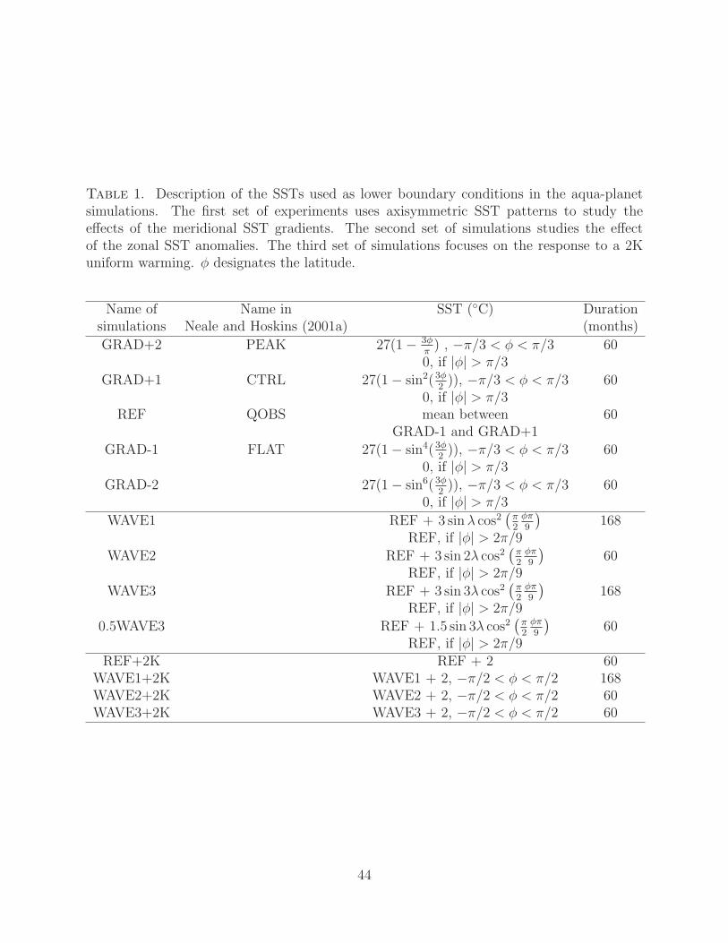
Table 1. Description of the SSTs used as lower boundary conditions in the aqua-planetsimulations. The first set of experiments uses axisymmetric SST patterns to study theeffects of the meridional SST gradients. The second set of simulations studies the effectof the zonal SST anomalies. The third set of simulations focuses on the response to a 2Kuniform warming. φ designates the latitude.
Name of Name in SST (◦C) Durationsimulations Neale and Hoskins (2001a) (months)
GRAD+2 PEAK 27(1 − 3φ
π) , −π/3 < φ < π/3 60
0, if |φ| > π/3
GRAD+1 CTRL 27(1 − sin2(3φ
2)), −π/3 < φ < π/3 60
0, if |φ| > π/3REF QOBS mean between 60
GRAD-1 and GRAD+1
GRAD-1 FLAT 27(1 − sin4(3φ
2)), −π/3 < φ < π/3 60
0, if |φ| > π/3
GRAD-2 27(1 − sin6(3φ
2)), −π/3 < φ < π/3 60
0, if |φ| > π/3
WAVE1 REF + 3 sin λ cos2(
π2
φπ
9
)
168REF, if |φ| > 2π/9
WAVE2 REF + 3 sin 2λ cos2(
π2
φπ
9
)
60REF, if |φ| > 2π/9
WAVE3 REF + 3 sin 3λ cos2(
π2
φπ
9
)
168REF, if |φ| > 2π/9
0.5WAVE3 REF + 1.5 sin 3λ cos2(
π2
φπ
9
)
60REF, if |φ| > 2π/9
REF+2K REF + 2 60WAVE1+2K WAVE1 + 2, −π/2 < φ < π/2 168WAVE2+2K WAVE2 + 2, −π/2 < φ < π/2 60WAVE3+2K WAVE3 + 2, −π/2 < φ < π/2 60
44

Table 2. Hadley and Walker circulations in the aqua-planet simulations. The differencesbetween the control and +2K simulations, and between 0.5WAVE3 and WAVE3 are given.σ is the monthly standard deviation. The p-values of the student t-test test the differencesof the means, the degree of freedom being calculated with the number of monthly outputs.max(ψ) and max(ψ∗
x) are respectively the maximum meridional streamfunction and zonalstreamfunction anomalies, averaged between 700-hPa and 300-hPa. δχ200 and δSLP des-ignate respectively the Walker circulation intensity described by the velocity potential at200-hPa and SLP zonal gradients, averaged between 5◦N and 5◦S.
Simulations REF/ WAVE1/ WAVE2/ WAVE3/ WAVE3/REF+2K WAVE1+2K WAVE2+2K WAVE3+2K 0.5WAVE3
max(ψ) ±σ 15.9 ± 0.8 7.7 ± 0.6 8.6 ± 0.8 10.7 ± 1.1(1010 kg s−1)∆ψ (1010 kg s−1) -0.6 +0.2 +0.1 +0.4 +0.9∆ψ/ψ (%) -4.0% +3.3% +1.7% +3.8% +8.2%p-value student t-test 0.00 0.02 0.23 0.00 0.00max(ψ∗
x) ±σ 3.2 ± 0.8 9.8 ± 1.0 6.8 ± 0.8 4.2 ± 0.7(1010 kg s−1)∆ψ∗
x (1010 kg s−1) +0.3 +0.6 +0.3 -0.1 -0.4∆ψ∗
x/ψ∗
x (%) +10.0% +6.1% +3.9% -2.5% -8.8%p-value student t-test 0.01 0.00 0.05 0.21 0.00δχ200 ±σ 7.6 ± 0.2 13.7 ± 0.1 18.4 ± 0.1 21.2 ± 0.1(106 m2 s−1)∆χ200 (106 m2 s−1) +0.6 -0.2 -0.3 -0.6 -1.5∆χ200/χ200 (%) +6.1% -2.3% -3.5% -0.6% -15.0%p-value student t-test 0.13 0.13 0.02 0.32 0.00δSLP ±σ 98 ± 31 718 ± 57 511 ± 38 439 ± 27(Pa)∆δSLP (Pa) 0 8 2 -8 -220∆δSLP/δSLP (%) -0.0% +1.2% +0.3% -2.0% -50.0%p-value student t-test 0.39 0.25 0.38 0.00 0.00
45

List of Figures
1 Sea Surface Temperature (◦K) and zonal-mean precipitation (mm d−1). (top
left) SST and (top right) zonal-mean precipitation for the simulations where
the meridional SST gradients are modified; (bottom left) SST anomalies in
WAVE3 and (bottom right) zonal-mean precipitation in simulations with
zonal SST anomalies. 51
2 Mean meridional streamfunction, in 1010 kg s−1 (contours), and zonal-mean
zonal wind, in m s−1 (shades). 52
3 Hadley cell and jet stream characteristics. (top) Intensity and (bottom) lati-
tudinal position in degree latitude of the Hadley cell and jet stream, for (left)
simulations with different meridional SST gradients and (right) simulations
with SST zonal anomalies. The latitudinal position of the jet streams is given
by the location of the maximum zonal-mean zonal wind. The position of the
subtropical and eddy-driven jets are given by the location of the maximum
convergence flux of momentum by the zonal mean circulation and eddies (see
Eqs. (3) and (4)). 53
4 Stationary eddy response to the zonal SST anomalies, for the simulation
WAVE2. Left panel shows the geopotential anomalies in m (thin contours),
the anomalous flow at the 200-hPa level, in m s−1 (vectors), and the zonal
SST anomalies, in ◦K (thick contours). Right panel shows the zonal-mean
stationary horizontal momentum transport in m2 s−2. 54
46

5 Geopotential anomalies in m (contours), the anomalous flow at the 200-hPa
level, in m s−1 (vectors), and longitudinal SST anomalies in ◦K (thick con-
tours) for the simulations (left) WAVE1 and (right) WAVE3. 55
6 Velocity potential at the 200-hPa height, χ200, in 105 m2s−1, in thin con-
tours, for the simulation WAVE1 (upper-left panel), WAVE2 (upper-right)
and WAVE3 (lower panels). The differences WAVE1+2K-WAVE1 (upper-
left),WAVE2+2K-WAVE2 (upper-right), WAVE3+2K-WAVE3 (lower-left) and
0.5WAVE3-WAVE3 (lower-right) are shown in colors shades. The zonal SST
anomalies are shown with thick contours. 56
7 Mean zonal streamfunction anomalies over the domain of the Hadley cells,
in contours, for WAVE1 (top-left panel), WAVE2 (top-right) and WAVE3
(bottom left and right) simulations, in 1010 kg s−1. The colors show the
differences WAVE1+2K-WAVE1 (top-left panel), WAVE2+2K-WAVE2 (top-
right), WAVE3+2K-WAVE3 (bottom-left) and 0.5WAVE3-WAVE3 (bottom-
right). 57
8 Mean meridional streamfunction in contours, in 1010 kg s−1 in REF+2K (top-
left panel), WAVE1+2K (top-right), WAVE3+2K (bottom-left) and WAVE3
(bottom-right). The colors show the differences REF+2K-REF(top-left panel),
WAVE1+2K-WAVE1 (top-right), WAVE3+2K-WAVE3 (bottom-left) and 0.5WAVE3-
WAVE3 (bottom-right). 58
47

9 Scatter plots illustrating the mean thermodynamic state of the tropical atmo-
sphere. (upper panel) Column integrated water vapor, W, versus 500-hPa dry
static stability, Sp500. (middle panel) Dry static stability at 500-hPa versus
mean ascending mid-tropospheric velocity, M+
500. (lower panel) Precipitation,
P, versus mean ascending mid-tropospheric velocity, M+
500. All variables are
averaged over the domain of the Hadley cells. 59
10 Zonal-mean zonal wind balance at the 200-hPa height, and contribution to
the wind tendency in m s−1 day−1 from the mean advection, Coriolis torque,
stationary and transient eddies. The continuous lines designate the results
for the simulation REF, while the dashed lines indicate the results of the
simulations GRAD-2 (top panel) and WAVE3 (bottom panel). 60
11 Zonal-mean MSE total flux, for the REF simulation, and decomposition into
latent heat and DSE fluxes. The position of the Hadley cell, for REF, indi-
cated by the latitude of the maximum (zero-value) meridional streamfunction,
averaged between 300-hPa and 700-hPa, is shown with a thin (thick) black
dashed vertical line. 61
12 Zonal-mean MSE flux, and decomposition into mean, transient and station-
ary components. The REF simulation is shown with dashed lines, while the
GRAD+2 (top-left panel), GRAD-2 (top-right panel), WAVE3 (bottom-left
panel) and REF+2K (bottom-right panel) are represented with continuous
lines. The position of the Hadley cell, for REF, indicated by the latitude
of the maximum (zero-value) meridional streamfunction, averaged between
300-hPa and 700-hPa, is shown with a thin (thick) black dashed vertical line. 62
48

13 Different terms of the zonal-mean MSE budget: LvE, the turbulent latent
heat flux, QR, the radiative cooling, H, the turbulent sensible heat flux and
total, QR + H + LvE. The REF simulation is shown with dashed lines, while
the GRAD+2 (top-left panel), GRAD-2 (top-right panel), REF+2K (bottom-
left panel) and WAVE2 (bottom-right panel) are represented with continuous
lines. The position of the Hadley cell, for REF, indicated by the latitude of the
maximum (zero-value) meridional streamfunction, averaged between 300-hPa
and 700-hPa, is shown with a thin (thick) black dashed vertical line. 63
14 Deviation from the zonal-mean for the different terms of the meridional-mean
MSE budget, averaged over the domain of the Hadley cells. LvE is the tur-
bulent latent heat flux, H, the turbulent sensible heat flux, QR, the radiative
heating of the atmospheric column. Total designates the sum QR +H +LvE.
The continuous line illustrates the results for WAVE1+2K (upper panel),
WAVE3+2K (middle panel) and 0.5WAVE3 (lower panel), while the dashed
lines are for WAVE1 (upper panel) and WAVE3 (middle and lower panels). 64
15 Zonal-mean gross moist stability, in kJ kg−1, in simulations using different
meridional SST gradients (upper panel), uniform warming simulations (middle
panel) and simulations with zonal SST anomalies (lower panel). 65
16 Intensity of the mean meridional circulation ψ, total MSE flux F , fraction
of the MSE flux transported by the mean meridional circulation C and gross
moist static stability ∆m. The values are averaged over the deep tropics (be-
tween 2.5◦ and 15◦). The errors bars show the monthly standard deviations. 66
49
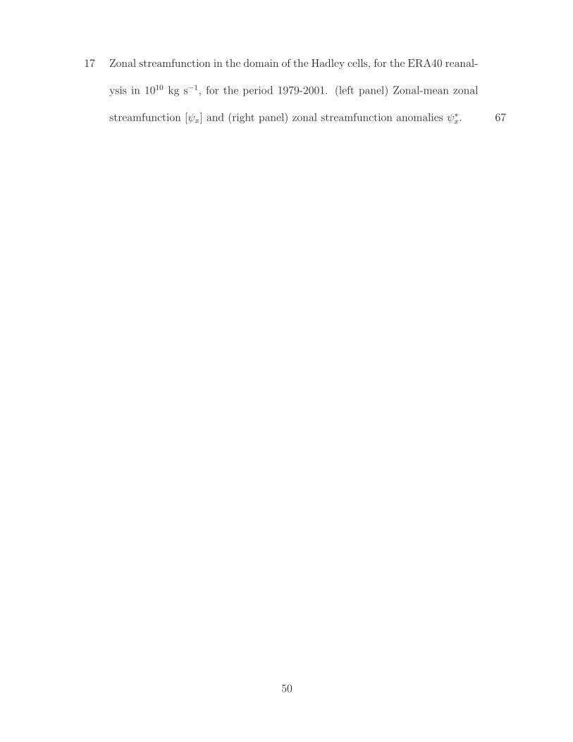
17 Zonal streamfunction in the domain of the Hadley cells, for the ERA40 reanal-
ysis in 1010 kg s−1, for the period 1979-2001. (left panel) Zonal-mean zonal
streamfunction [ψx] and (right panel) zonal streamfunction anomalies ψ∗
x. 67
50
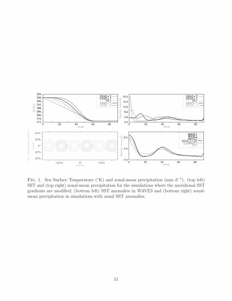
Fig. 1. Sea Surface Temperature (◦K) and zonal-mean precipitation (mm d−1). (top left)SST and (top right) zonal-mean precipitation for the simulations where the meridional SSTgradients are modified; (bottom left) SST anomalies in WAVE3 and (bottom right) zonal-mean precipitation in simulations with zonal SST anomalies.
51
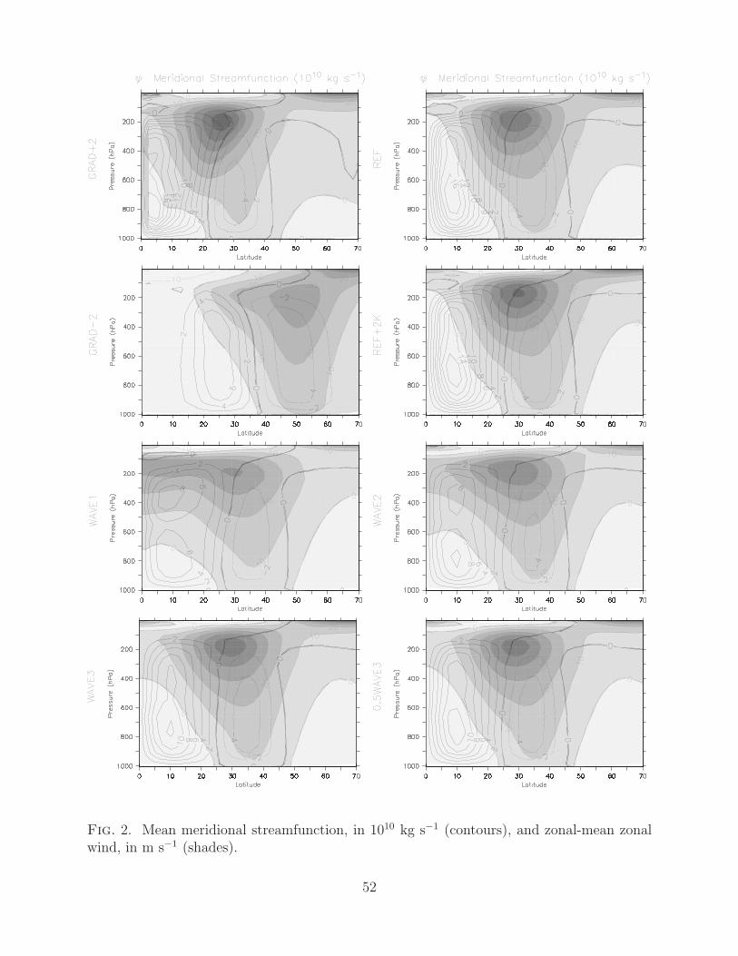
Fig. 2. Mean meridional streamfunction, in 1010 kg s−1 (contours), and zonal-mean zonalwind, in m s−1 (shades).
52
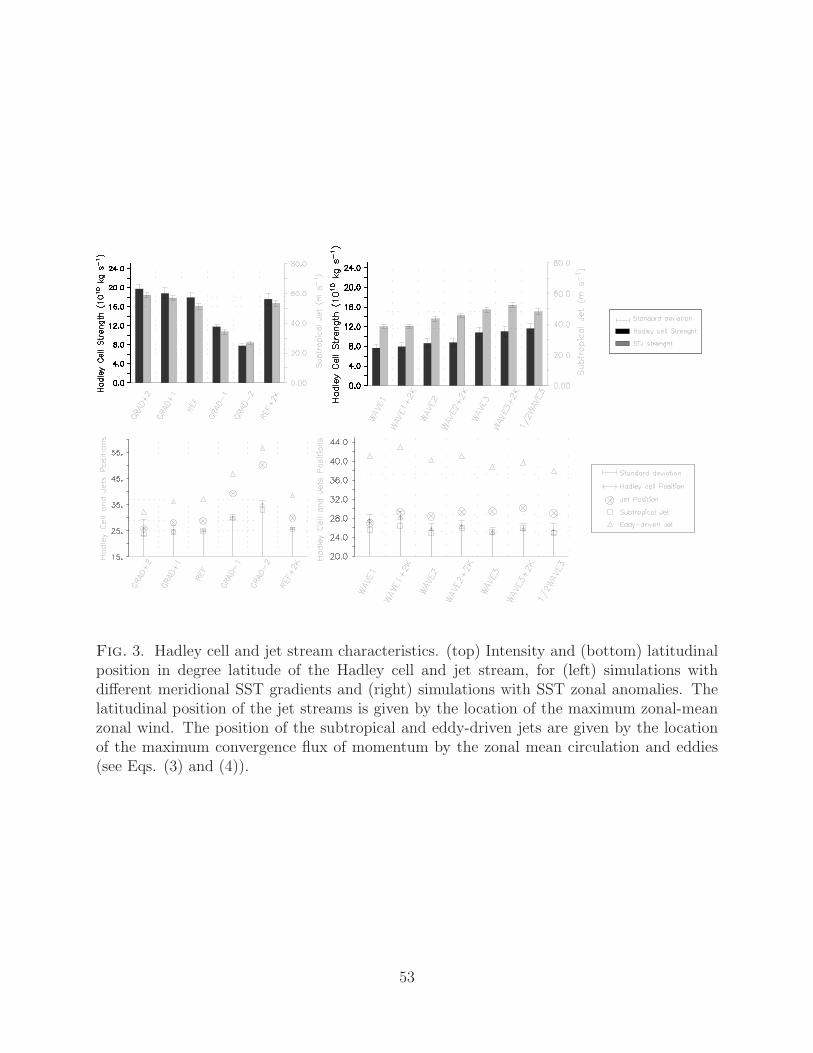
Fig. 3. Hadley cell and jet stream characteristics. (top) Intensity and (bottom) latitudinalposition in degree latitude of the Hadley cell and jet stream, for (left) simulations withdifferent meridional SST gradients and (right) simulations with SST zonal anomalies. Thelatitudinal position of the jet streams is given by the location of the maximum zonal-meanzonal wind. The position of the subtropical and eddy-driven jets are given by the locationof the maximum convergence flux of momentum by the zonal mean circulation and eddies(see Eqs. (3) and (4)).
53

Fig. 4. Stationary eddy response to the zonal SST anomalies, for the simulation WAVE2.Left panel shows the geopotential anomalies in m (thin contours), the anomalous flow atthe 200-hPa level, in m s−1 (vectors), and the zonal SST anomalies, in ◦K (thick contours).Right panel shows the zonal-mean stationary horizontal momentum transport in m2 s−2.
54
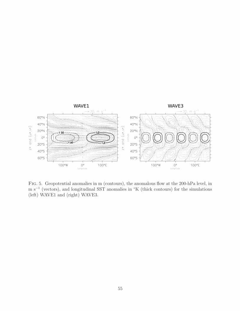
Fig. 5. Geopotential anomalies in m (contours), the anomalous flow at the 200-hPa level, inm s−1 (vectors), and longitudinal SST anomalies in ◦K (thick contours) for the simulations(left) WAVE1 and (right) WAVE3.
55

Fig. 6. Velocity potential at the 200-hPa height, χ200, in 105 m2s−1, in thin contours, forthe simulation WAVE1 (upper-left panel), WAVE2 (upper-right) and WAVE3 (lower pan-els). The differences WAVE1+2K-WAVE1 (upper-left),WAVE2+2K-WAVE2 (upper-right),WAVE3+2K-WAVE3 (lower-left) and 0.5WAVE3-WAVE3 (lower-right) are shown in colorsshades. The zonal SST anomalies are shown with thick contours.
56

Fig. 7. Mean zonal streamfunction anomalies over the domain of the Hadley cells, incontours, for WAVE1 (top-left panel), WAVE2 (top-right) and WAVE3 (bottom left andright) simulations, in 1010 kg s−1. The colors show the differences WAVE1+2K-WAVE1(top-left panel), WAVE2+2K-WAVE2 (top-right), WAVE3+2K-WAVE3 (bottom-left) and0.5WAVE3-WAVE3 (bottom-right).
57

Fig. 8. Mean meridional streamfunction in contours, in 1010 kg s−1 in REF+2K (top-leftpanel), WAVE1+2K (top-right), WAVE3+2K (bottom-left) and WAVE3 (bottom-right).The colors show the differences REF+2K-REF(top-left panel), WAVE1+2K-WAVE1 (top-right), WAVE3+2K-WAVE3 (bottom-left) and 0.5WAVE3-WAVE3 (bottom-right).
58
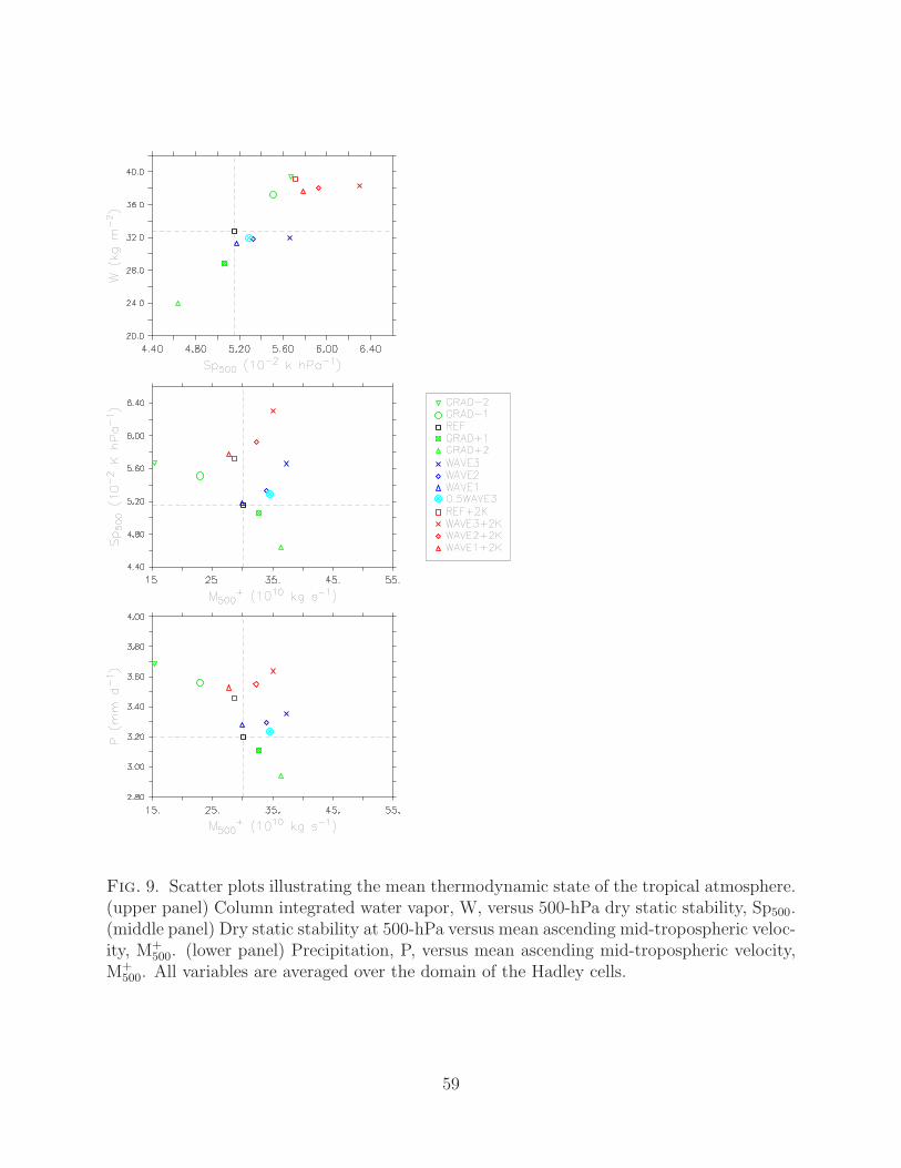
Fig. 9. Scatter plots illustrating the mean thermodynamic state of the tropical atmosphere.(upper panel) Column integrated water vapor, W, versus 500-hPa dry static stability, Sp500.(middle panel) Dry static stability at 500-hPa versus mean ascending mid-tropospheric veloc-ity, M+
500. (lower panel) Precipitation, P, versus mean ascending mid-tropospheric velocity,M+
500. All variables are averaged over the domain of the Hadley cells.
59

Fig. 10. Zonal-mean zonal wind balance at the 200-hPa height, and contribution to thewind tendency in m s−1 day−1 from the mean advection, Coriolis torque, stationary andtransient eddies. The continuous lines designate the results for the simulation REF, whilethe dashed lines indicate the results of the simulations GRAD-2 (top panel) and WAVE3(bottom panel).
60
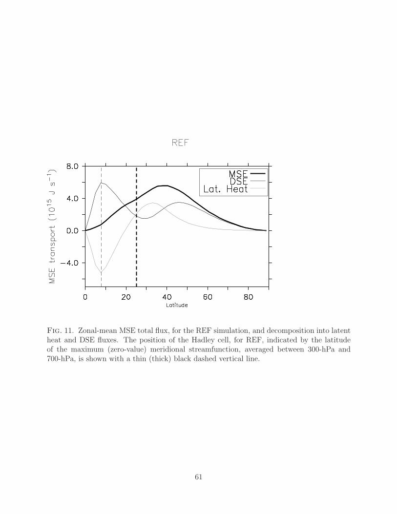
Fig. 11. Zonal-mean MSE total flux, for the REF simulation, and decomposition into latentheat and DSE fluxes. The position of the Hadley cell, for REF, indicated by the latitudeof the maximum (zero-value) meridional streamfunction, averaged between 300-hPa and700-hPa, is shown with a thin (thick) black dashed vertical line.
61

Fig. 12. Zonal-mean MSE flux, and decomposition into mean, transient and stationarycomponents. The REF simulation is shown with dashed lines, while the GRAD+2 (top-leftpanel), GRAD-2 (top-right panel), WAVE3 (bottom-left panel) and REF+2K (bottom-rightpanel) are represented with continuous lines. The position of the Hadley cell, for REF,indicated by the latitude of the maximum (zero-value) meridional streamfunction, averagedbetween 300-hPa and 700-hPa, is shown with a thin (thick) black dashed vertical line.
62
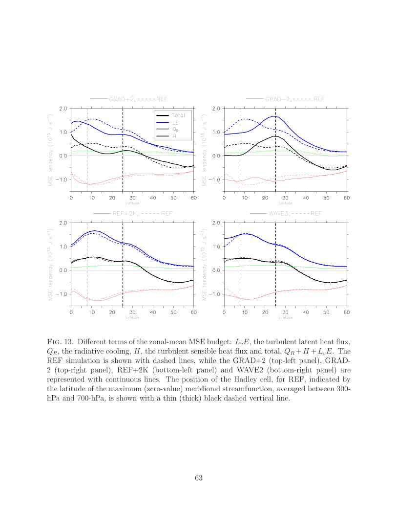
Fig. 13. Different terms of the zonal-mean MSE budget: LvE, the turbulent latent heat flux,QR, the radiative cooling, H, the turbulent sensible heat flux and total, QR +H +LvE. TheREF simulation is shown with dashed lines, while the GRAD+2 (top-left panel), GRAD-2 (top-right panel), REF+2K (bottom-left panel) and WAVE2 (bottom-right panel) arerepresented with continuous lines. The position of the Hadley cell, for REF, indicated bythe latitude of the maximum (zero-value) meridional streamfunction, averaged between 300-hPa and 700-hPa, is shown with a thin (thick) black dashed vertical line.
63
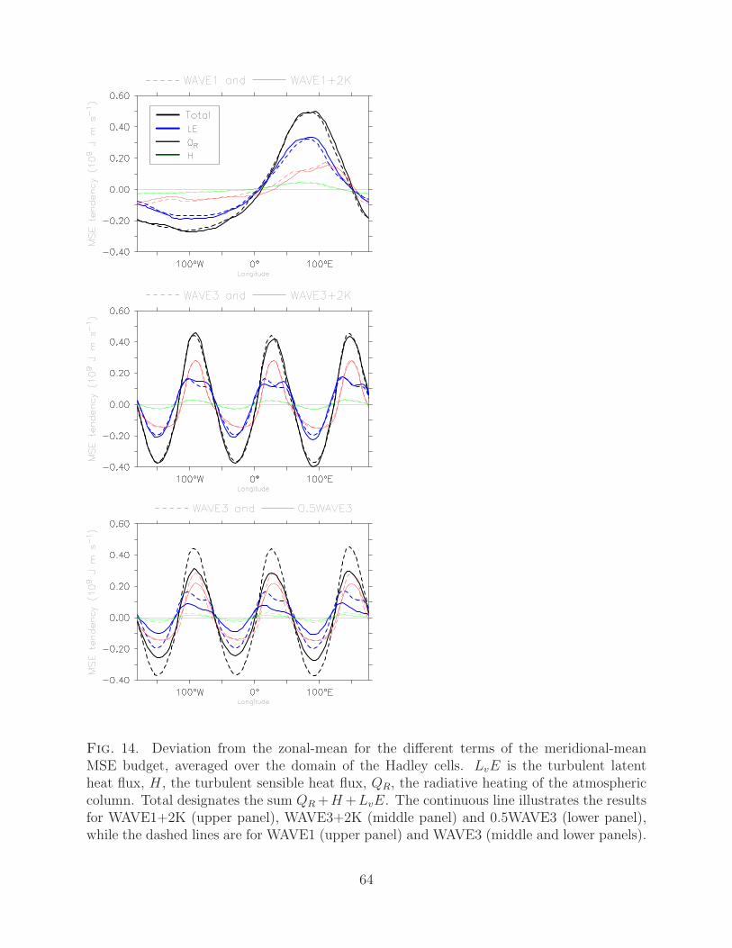
Fig. 14. Deviation from the zonal-mean for the different terms of the meridional-meanMSE budget, averaged over the domain of the Hadley cells. LvE is the turbulent latentheat flux, H, the turbulent sensible heat flux, QR, the radiative heating of the atmosphericcolumn. Total designates the sum QR +H +LvE. The continuous line illustrates the resultsfor WAVE1+2K (upper panel), WAVE3+2K (middle panel) and 0.5WAVE3 (lower panel),while the dashed lines are for WAVE1 (upper panel) and WAVE3 (middle and lower panels).
64
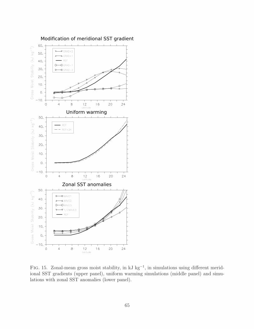
Fig. 15. Zonal-mean gross moist stability, in kJ kg−1, in simulations using different merid-ional SST gradients (upper panel), uniform warming simulations (middle panel) and simu-lations with zonal SST anomalies (lower panel).
65

Fig. 16. Intensity of the mean meridional circulation ψ, total MSE flux F , fraction of theMSE flux transported by the mean meridional circulation C and gross moist static stability∆m. The values are averaged over the deep tropics (between 2.5◦ and 15◦). The errors barsshow the monthly standard deviations.
66

Fig. 17. Zonal streamfunction in the domain of the Hadley cells, for the ERA40 reanalysisin 1010 kg s−1, for the period 1979-2001. (left panel) Zonal-mean zonal streamfunction [ψx]and (right panel) zonal streamfunction anomalies ψ∗
x.
67