guilherme ferreira da costa - repositório da universidade...
TRANSCRIPT

Instituto Superior de Ciencias do Trabalho e da Empresa
Faculdade de Ciencias da Universidade de Lisboa
Departamento de Financas do ISCTE
Departamento de Matematica da FCUL
ALTERNATIVE STRUCTURAL MODELS TO APPROXIMATE
MOODY’S KMV DISTANCE TO DEFAULT
Guilherme Ferreira da Costa
A Dissertation presented in partial fulfillment of the Requirements for the Degree of
Master in Financial Mathematics
October 2011

Instituto Superior de Ciencias do Trabalho e da Empresa
Faculdade de Ciencias da Universidade de Lisboa
Departamento de Financas do ISCTE
Departamento de Matematica da FCUL
ALTERNATIVE STRUCTURAL MODELS TO APPROXIMATE
MOODY’S KMV DISTANCE TO DEFAULT
Guilherme Ferreira da Costa
A Dissertation presented in partial fulfillment of the Requirements for the Degree of
Master in Financial Mathematics
Dissertation supervised by
Professor Doutor Joao Pedro Pereira
October 2011


Resumo
Esta tese compara o uso de diferentes modelos estruturais para estimacaodos activos de uma empresa e da da volatilidade dos mesmos, de modo a cal-cular o correspondente valor da Distance to Default, tal como definido pelaMoody’s KMV. A abordagem utilizada consiste em implementar a estimacaode metodos baseados no modelo de Black-Scholes e no modelo CEV. Estesmetodos sao seguidamente utilizados para determinar os valores da Distance
to Default para uma amostra de empresas, de modo a encontrar o metodoque melhor aproxima os valores da Moody’s KMV. Alguns dos resultadosobtidos foram melhores que os do modelo padrao, o modelo Black-Scholes.O uso de um modelo baseado em interpretar o valor de mercado da empresacomo uma opcao do tipo Down and Out Call sobre os activos da empresa,os quais se determinou seguirem o modelo CEV Square Root, e em postulardirectamente uma relacao funcional entre a volatilidade dos activos da em-presa e a volatilidade do valor da empresa em mercado, mostrou resultadossubstancialmente melhores que os restantes modelos.
Palavras-Chave: Moody’s KMV, Distance to Default, Modelo Black-Sholes, Modelo CEV.


Abstract
This thesis compares the use of different structural models in order to esti-mate a firm’s assets and asset’s volatility values and compute the correspond-ing Distance to Default value as defined by Moody’s KMV. The approachused consists in implementing estimation methods based on the Black-ScholesModel and the Constant Elasticity of Variance Model. These methods arethen applied to determine the Distance to Default values from a sample offirms, in search for the method that better approximates Moody’s KMV val-ues. Some of the results obtained were better than the benchmark model, theBlack-Scholes model. The use of a model based on interpreting equity as one-year Down and Out Call Option on the firm’s assets who were determined tofollow a CEV Square Model and on postulating directly a functional relationbetween the firm’s asset’s volatility and equity volatility, showed substan-tially better results than the remaining models.
Key-words: Moody’s KMV, Distance to Default, Black-Sholes Model,CEV Model.
i

Acknowledgments
I am deeply indebted to my supervisor Joao Pedro Pereira for its constantsupport during the writing of this thesis.
I would like to thank professor Joao Pedro Nunes for the time sparedhelping me with questions regarding the CEV model.
I am also very grateful to my uncle Ricardo Severino and aunt JoanaSoares and to my cousin Emılia Ataıde for their comments and suggestions.
ii
Contents
1 Moody’s KMV Expected Default Frequency and Distance toDefault 31.1 Estimating the firm’s assets value and volatility . . . . . . . . 31.2 Calculating the distance to default . . . . . . . . . . . . . . . 41.3 Mapping the Distance to Default to the probability of default 4
2 Theoretical Models 52.1 General Considerations . . . . . . . . . . . . . . . . . . . . . . 52.2 Black-Scholes Model . . . . . . . . . . . . . . . . . . . . . . . 6
2.2.1 Black-Scholes Model - 1 year - without default . . . . . 62.2.2 Black-Scholes Model - 1 year - with default . . . . . . . 7
2.3 CEV Square Root Model . . . . . . . . . . . . . . . . . . . . . 92.3.1 CEV Model - 1 year - without default . . . . . . . . . . 92.3.2 CEV Model - 1 year - with default . . . . . . . . . . . 102.3.3 CEV Model - 10 years - with default . . . . . . . . . . 11
3 Numerical Results 133.1 Sample and Moody’s KMV results . . . . . . . . . . . . . . . 133.2 Black-Scholes Model . . . . . . . . . . . . . . . . . . . . . . . 15
3.2.1 Black-Scholes Model - 1 year - without default . . . . . 153.2.2 Black-Scholes Model - 1 year - with default . . . . . . . 17
3.3 CEV Model . . . . . . . . . . . . . . . . . . . . . . . . . . . . 193.3.1 CEV Model - 1 year - without default . . . . . . . . . . 193.3.2 CEV Model - 1 year - with default . . . . . . . . . . . 213.3.3 CEV Model - 10 year - with default . . . . . . . . . . . 25
3.4 Comparison of the Models . . . . . . . . . . . . . . . . . . . . 27
4 Conclusion 29
iii

A Auxiliary Results 30A.1 Derivation of Black-Scholes δ . . . . . . . . . . . . . . . . . . 30
B Auxiliary Tables 31B.1 Firms used in the sample . . . . . . . . . . . . . . . . . . . . . 31
C Monte Carlo Methods 33C.1 ECEV (A,X, dp, r, τ) . . . . . . . . . . . . . . . . . . . . . . . . 33C.2 ECEV10(A, std, ltd, dp, r, τ) . . . . . . . . . . . . . . . . . . . . 34
iv

Introduction
Structural models have been in use for years as a basis for credit risk andcredit pricing models 1.
Moody’s KMV (MKVM) implements a modified structural model calledthe Vasicek-Kealhofer model, which allows for the estimation of the assetsand asset’s volatility of a publicly traded firm. These estimates are used byMKVM to compute a “distance to default” (DD) value for which it deter-mines an empirical distribution to generate the Expected Default Frequency(EDF) measure 2.
Due to commercial reasons, MKMV method is not fully disclosed. More-over, for many investors in need of estimating default probabilities or merelycomparing the risk of investing in different firms 3, replicating MKVMmethod-ology would be an impractically complex and time-consuming task and wouldrequire the use of MKVM proprietary defaults database.
This thesis addresses the problem of estimating MKMV DD using struc-tural models that result in methods different from the MKMV methodology.It proposes alternative structural models and analyses them in terms of: (a)their capacity for approximating DD values as computed by MKVM; (b) theircomputation time; (c) their ability to approximate MKVM EDF values.
The thesis is organized as follows. Chapter 1 describes MKMV generalframework for estimating default probabilities. It also contains MKVM DDdefinition, how to compute it and how to calculate its corresponding EDFmeasure.
Chapter 2 exposes the proposed structural models from a theoretical point
1See, for example, the description of the Merton and Vasicek-Kealhofer models presentin Arora et al. [2005].
2This is a commercially available estimate of a firm’s one-year default probability.3Note that it is theoretically possible to compare firms in terms of their default risk
without knowing their respective default probabilities.
1

of view. It describes in detail each of the model’s assumptions and motiva-tions and derives the corresponding formulas that allow us to estimate theassets and asset’s volatility values needed to compute a firm’s DD.
In Chapter 3 we test the models introduced in the previous chapter,using a sample obtained from MKMV of DD and EDF measures for differentfirms. We measure the difference between MKVM DD and EDF values andour models values for each of the firms in the sample. We then compare ourmodels based on these results and on their computation time.
Chapter 4 presents the thesis main conclusions.
2

Chapter 1
Moody’s KMV ExpectedDefault Frequency andDistance to Default
Moody’s KMV EDF (Expected Default Frequency) credit risk measures areforward-looking default probabilities estimates for public (and private) firms.Each EDF measure is determined in three steps:
1. Estimate the firm’s assets value and volatility;
2. Calculate the Distance to Default;
3. Map the Distance to Default to the probability of default.
1.1 Estimating the firm’s assets value and volatil-ity
In this step, for a publicly traded firm, asset value (A) and asset volatility(σA) are estimated from the market value of equity and book value of lia-bilities. In general, this can be achieved by choosing a structural model andusing an options pricing based approach, which recognizes equity as a calloption on the underlying assets of the firm 1. For this purpose, MKVM usesa version of the Vasicek-Kealhofer model, whose original formulation can befound in Vasicek [1984].
1See Merton [1974] for the seminal example.
3

1.2 Calculating the distance to default
Having estimated A and σA, MKVM computes the Distance to Defaulttrough the following formula 2:
DD =A− dp
AσA,
where dp denotes the default point.The default point is an estimate of the value for which if the firm’s assets
value falls bellow, the firm will default.It is important to stress that this is an estimate and that it does not
coincide with the value of the firm’s liabilities. As stated by MVMV [Crosbieand Bohn, 2003, p. 7], “in general firms do not default when their asset valuereaches the book value of their total liabilities. (...) The asset value the firmwill default, generally lies somewhere between total liabilities and current, orshort-term liabilities”.
1.3 Mapping the Distance to Default to theprobability of default
Usually, the estimates described in Section 1.2 would allow us to computea model implied default probability, either analytically or by using MonteCarlo Methods.
However, in the case of Moody’s KMV use of the Vasiceck-Kealhofermodel, default probabilities calculated in this manner “provide little dis-criminatory power” [Crosbie and Bohn, 2003, p. 14-18].
For this reason, EDF measures are computed using the DD empiricaldistribution. MKVM obtains a relationship between DD and default prob-ability from data on historical default: 3 for each DD value, the companyqueries the default history for the proportion of firms with this DD valuethat defaulted over the following year.
2To be precise, MKVM DD values depend on the time horizon we are considering:there is a DD value for each time horizon; the formula presented here is a one year DD.See the example from page 32 in Dwyer and Qu [2007].
3MKMV uses a database including over 250,000 company-years of data and over 4,700incidents of default or bankruptcy; see [Crosbie and Bohn, 2003, p. 14] and [Dwyer andQu, 2007, p. 22].
4

Chapter 2
Theoretical Models
2.1 General Considerations
In each section of this chapter, we will follow the methodology described inSection 1.1:
i. Describe equity as a call option on the underlying assets of the firm;
ii. Choose a structural model that posits a stochastic process for the valueof the firm’s assets and from which it is possible to derive a valuationformula for the option specified in i.;
iii. Write an equation using the option valuation formula from ii. that relatesA and σA with the firm’s equity (E), the firm’s equity volatility (σE) andthe risk-free interest rate (r); apply Ito’s lemma to the process from ii.or specify a functional relation between σA and σE in order to obtain thesecond equation needed to estimate A and σA.
The approach followed was to choose as structural models for step ii. theBlack-Scholes model, for being the simplest of the most widely used modelsin option valuation, and the Constant Elasticity of Variance (CEV) model 1.
The resulting empirical distribution of default probabilities as computedby MKMV has much wider tails than the Normal distribution resulting fromthe use of the Black-Scholes model 2. The CEV Model posits a distribution
1To be precise, we used a particular case of this model called the Constant Elasticityof Variance Square-Root Model.
2[Crosbie and Bohn, 2003, p. 18]
5

for the time t value of the assets that possess wider tails than the correspond-ing Lognormal distribution from the Black-Schols model. For this reason, theCEV model is a natural alternative to the Black-Scholes model. Moreover,the fact that it exhibits the so called leverage effect on volatility (the instan-taneous variance of stock returns being inversely related to the asset price)led us to formulate the hypothesis that this is a more powerful model for theestimation of default probabilities 3.
2.2 Black-Scholes Model
The Black-Scholes model posits that the market value of a firm’s underlyingassets (A) follows the following stochastic process:
dA = µAAdt+ σAAdz, (2.1)
where σA denotes the annualized volatility of the asset and dz is a standardBrownian motion.
2.2.1 Black-Scholes Model - 1 year - without default
In this section we assume that:
i. The firm’s assets follow the process described by Equation (2.1);
ii. All the firm’s debt is short-term debt with maturity equal to one year;
iii. There is no possibility of default occurring during the forthcoming year;
iv. In a year from now, it will be indifferent to an investor holding all thefirm’s equity or receiving the value of the firm’s assets minus the short-term debt that must be paid.
These assumptions imply that holding equity today is equivalent to holding acall option on the assets of the firm with strike price equal to the short-termdebt and maturity equal to one year. Using the Black-Scholes option pricingformula 4, we can therefore write
E = AN(d1)− e−rτstdN(d2), (2.2)
3The existence of this leverage effect on volatility is supported by several empiricalstudies: see, for instance, Beckers [1980] and Christie [1982].
4See Black and Scholes [1973].
6
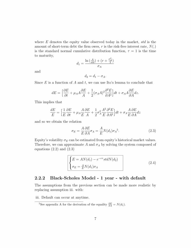
where E denotes the equity value observed today in the market, std is theamount of short-term debt the firm owes, r is the risk-free interest rate, N(.)is the standard normal cumulative distribution function, τ = 1 is the timeto maturity,
d1 =ln ( A
std) + (r +σ2A2 )
σA
andd2 = d1 − σA.
Since E is a function of A and t, we can use Ito’s lemma to conclude that
dE =�∂E∂t
+ µAA∂E
A+
1
2(σAA)
2∂2E
∂A2
�dt+ σAA
∂E
∂Adz.
This implies that
dE
E=
� 1E
∂E
∂t+ µA
A
E
∂E
A+
1
2σ2A
A2
E
∂2E
∂A2
�dt+ σA
A
E
∂E
∂Adz
and so we obtain the relation
σE =A
E
∂E
∂AσA =
A
EN(d1)σA
5. (2.3)
Equity’s volatility σE can be estimated from equity’s historical market values.Therefore, we can approximate A and σA by solving the system composed ofequations (2.2) and (2.3)
E = AN(d1)− e−rτstdN(d2)
σE = AEN(d1)σA
(2.4)
2.2.2 Black-Scholes Model - 1 year - with default
The assumptions from the previous section can be made more realistic byreplacing assumption iii. with:
iii. Default can occur at anytime.
5See appendix A for the derivation of the equality ∂E∂A = N(d1).
7
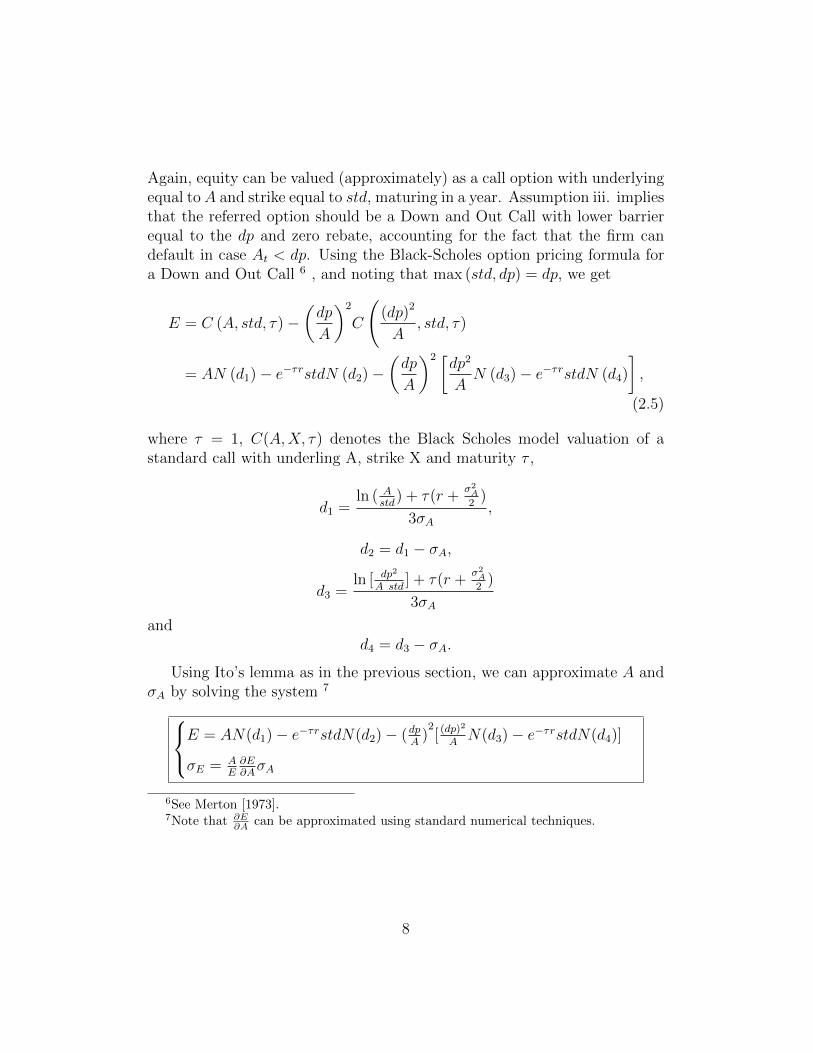
Again, equity can be valued (approximately) as a call option with underlyingequal to A and strike equal to std, maturing in a year. Assumption iii. impliesthat the referred option should be a Down and Out Call with lower barrierequal to the dp and zero rebate, accounting for the fact that the firm candefault in case At < dp. Using the Black-Scholes option pricing formula fora Down and Out Call 6 , and noting that max (std, dp) = dp, we get
E = C (A, std, τ)−�dp
A
�2
C
�(dp)2
A, std, τ)
= AN (d1)− e−τrstdN (d2)−�dp
A
�2 �dp2
AN (d3)− e−τrstdN (d4)
�,
(2.5)
where τ = 1, C(A,X, τ) denotes the Black Scholes model valuation of astandard call with underling A, strike X and maturity τ ,
d1 =ln ( A
std) + τ(r +σ2A2 )
3σA,
d2 = d1 − σA,
d3 =ln [ dp2
A std ] + τ(r +σ2A2 )
3σA
andd4 = d3 − σA.
Using Ito’s lemma as in the previous section, we can approximate A andσA by solving the system 7
E = AN(d1)− e−τrstdN(d2)− (dpA )
2[ (dp)
2
A N(d3)− e−τrstdN(d4)]
σE = AE
∂E∂AσA
6See Merton [1973].7Note that ∂E
∂A can be approximated using standard numerical techniques.
8
2.3 CEV Square Root Model
The Constant Elasticity of Variance (CEV) Square Root model posits thatthe market value of a firm’s underlying assets follows the following stochasticprocess:
dA = µAAdt+ δA√Adz. (2.6)
It follows immediately from the above equation that
σA =δA√A. (2.7)
2.3.1 CEV Model - 1 year - without default
The assumptions made in this section are the same as the ones described inSection 2.2.1, except for statement i., which we now replace with
i. The firm’s assets follow the process described in (2.6).
Again, these assumptions imply that holding equity today is equivalent toholding a call option on the assets of the firm with strike price equal tothe short-term debt and maturity equal to one year. Using the CEV modeloption pricing formula 8, we can therefore write
E = AQχ2(4,2x)(2k std)− std e−rτ [1−Qχ2(2,2kX)(2x)], (2.8)
where Q2χ(a, b) denotes the complementary distribution function of a random
variable that follows a non-central Chi-squared law with a degrees of freedomand no-centrality parameter b, τ = 1 is the time to maturity of the option,
k :=2r
δ2A(erτ − 1)
,
andx := kAerτ .
Applying Ito’s Lemma we can conclude that:
dE =�∂E∂t
+ µAA∂E
A+
1
2(δA
√A)2
∂2E
∂A2
�dt+ δA
√A∂E
∂Adz.
8See Cox [1975].
9
This implies that
dE
E=
� 1E
∂E
∂t+ µA
A
E
∂E
A+
1
2δ2A
A
E
∂2E
∂A2
�dt+ δA
√A
E
∂E
∂Adz
and so we obtain the relation
σE =
√A
E
∂E
∂AδA. (2.9)
As in the previous chapter, we can approximate A and δA by solving thesystem composed of equations (2.8) and (2.9)
E = AQχ2(4,2x)(2k std)− std e−rτ [1−Qχ2(2,2kX)(2x)]
σE =√AE
∂E∂AδA
(2.10)
After approximating A and δA, an estimate of σA can be obtained troughEquation (2.7).
2.3.2 CEV Model - 1 year - with default
In this section it is assumed that:
i. The firm’s assets follow the process described by Equation (2.6);
ii. All the firm’s debt is short-term debt with maturity equal to one year;
iii. Default can occur at anytime.
iv. In a year from now, it will be indifferent to an investor holding all thefirm’s equity or receiving the value of the firm’s assets minus the short-term debt that must be paid.
Henceforth, ECEV (A,X, dp, r, τ) denotes the computed value of a Euro-pean Down and Out Call option with an underlying A following the processdescribed by Equation (2.6), strike X, lower barrier dp, maturity τ = 1, zerorebate and risk-free rate r. This value is computed using a Monte Carlomethod, detailed in appendix C.
The use of Monte Carlo Methods for the valuation of E implies thatthe time required to compute ∂E
∂A numerically makes it unfeasible the useof Equation (2.9). Consequently, the approach followed was to postulatedirectly the functional relation supposed to exist between σA and σE.
In order to do this, it is necessary to add to our list of assumptions:
10
vi. Equity also follows a CEV Square Root Model of the type described byEquation (2.8);
vii. δA ≈ δE.
Since assumption vi. implies that σE = δE√E
and consequently that δE =
σE
√E, we can approximate δA using assumption vii:
δA ≈ δE = σE
√E. (2.11)
Regarding assumption vii., it is worth noting that it is well known thatin general σA < σE
9. What we are assuming, recurring here to Equation(2.9), is that σA < σE due to the fact that we usually have A > E. We seeno reason to believe the way σA changes with A, is in any aspect, differentfrom the way σE varies with E.
Since equity can be seen as a Down and Out Call Option with zero rebate,as was done in Section 2.2.2, and using Equation (2.11), we can write
E = ECEV (A, std, dp, r, τ)
δA = σE
√E
(2.12)
2.3.3 CEV Model - 10 years - with default
In this section we consider a more realistic picture of a firm’s debt structureby defining two classes of debt: short-term debt and long-term debt.
The assumptions made are the following:
i. The firm’s assets follow the process described by Equation (2.6);
ii. The firm’s debt consists of short-term debt (std), maturing in one year,and long-term debt (ltd), which we assume will mature in ten years;
iii. Default can occur at anytime;
iv. In ten years from now, it will be indifferent to an investor holding all thefirm’s equity or receiving the value of the firm’s assets minus ltd;
9See for instance Crosbie and Bohn [2003]
11
v. Equity follows a CEV Square Root Model of the type described by Equa-tion (2.8);
vi. δA ≈ δE.
It is worth noting that the above assumptions imply the following:
a) If somewhere between now and a year from now we have At < dp, ourfirms defaults;
b) In a year from now, our firm will have to pay the short-term debt std,implying that A1 will be replaced by A1 − std and dp by dp− std;
c) After reaching year one and paying std, we can approximate equity’svalue by that of a European Down and Out Call option with underlying(A− dp), strike ltd, lower barrier (dp− std), maturity τ = 9, zero rebateand risk-free rate r.
From statements a), b) and c), it is possible to value equity’s present valueusing Monte Carlo methods, as described in Appendix C .
Representing these valuation by E = ECEV10(A, std, ltd, dp, r, τ) we canthen solve, as in the previous section, the following equations:
E = ECEV10(A, std, ltd, dp, r, τ)
δA = σE
√E
(2.13)
As stated before, after estimating δA, σA can be approximated trough Equa-tion (2.7).
12

Chapter 3
Numerical Results
3.1 Sample and Moody’s KMV results
The models described in Chapter one were applied to a sample of 20 firms,whose relevant financial data, as supplied by Moody’s KMV, is summarizedbelow in Table 3.1. E denotes the firm’s equity, σE, its equity volatility, stdthe short-term debt, dp the firm’s default-point and r its risk-free rate.
Each firm is identified with an abbreviated name. For the firm’s completename, as well as the date to which the presented data refers to, see appendixB.
All default probabilities presented were computed using Monte Carlomethods, generating for each computation n = 1000 sample paths, eachwith 120 equally spaced points.
13

Table 3.1: Sample Data
E σE total debt std dp rNRTLQ 6599.295 47.74% 14170 6481 10325 3.41%FRP 634.72 47.72% 2758.782 308.638 1931.147 3.07%SPCB 245.357 90.39% 3146.126 606.156 2202.288 2.69%LEAR 1990.578 50.92% 6924.567 3921.7 5423.133 3.84%TROXA 335.68 51.40% 1238.3 408.7 866.81 1.93%PGPDQ 1976.713 33.44% 2746.79 948.269 1922.753 4.53%VSUNQ 1057.599 44.03% 755.771 97.428 529.04 2.45%FNM 63780.203 27.01% 802294 335618 568956 4.90%8868 429.522 45.32% 338.687 212.573 275.63 5.01%ANS 109.87 65.04% 1110.947 83.949 777.663 3.08%SIX 584.243 49.22% 2463.2 291.421 1724.24 5.50%PRTL 79.32 124.41% 862.423 253.411 603.696 5.38%VRSO 0.57 2636.93% 35.699 30.466 33.083 2.48%IREP 0.34 8470.44% 135.488 124.998 130.243 2.50%TMBAF 37.67 226.67% 1965 501 1375.5 2.72%TOUS 9.24 1226.35% 2243.4 519 1570.38 2.69%WOLV 3.95 143.93% 7.49 6.422 6.956 5.45%BFTH 26.92 168.19% 1845.17 437.781 1291.619 5.32%NEWC 92.64 190.52% 22995.418 12646.253 17820.836 5.26%TRINQ 1.57 1107.18% 49.856 49.426 18.471 5.37%
14

Moody’s KMV Model results for this given sample are presented bellow.
Table 3.2: Moody’s KMV
A σA DD EDFNRTLQ 19515.295 19.23% 2.45 0.0128FRP 2824.308 17.16% 1.84 0.0445SPCB 2486.701 18.25% 0.63 0.2479LEAR 8383.416 14.95% 2.36 0.0185TROXA 1380.905 17.55% 2.12 0.0269PGPDQ 4711.857 15.41% 3.84 0.0019VSUNQ 1753.849 28.18% 2.48 0.0057FNM 872775.125 4.55% 7.65 0.0058868 735.261 27.56% 2.27 0.0103ANS 998.29 15.43% 1.43 0.0861SIX 3023.065 16.90% 2.54 0.0143PRTL 704.127 23.38% 0.61 0.2563VRSO 33.669 45.93% 0.04 0.35IREP 130.6 23.13% 0.01 0.35TMBAF 1341.097 16.98% 0.00 0.35TOUS 1405.017 20.53% 0.00 0.35WOLV 11.807 55.81% 0.74 0.2BFTH 1300.774 16.10% 0.04 0.2NEWC 18708.627 7.47% 0.64 0.2TRINQ 51.218 34.09% 1.88 0.2
3.2 Black-Scholes Model
3.2.1 Black-Scholes Model - 1 year - without default
Table 3.3 shows the results obtained for this model.
15

Table 3.3: Black-Scholes - 1 year - without default
A σA DD pNRTLQ 20289.3504 0.1560 3.1479 0FRP 3309.0899 0.0924 4.5063 0SPCB 3275.0752 0.0849 3.8569 0LEAR 8649.8835 0.1186 3.1454 0TROXA 1549.4566 0.1129 3.9033 0PGPDQ 4601.8443 0.1436 4.0529 0VSUNQ 1795.0556 0.2595 2.7182 0FNM 827709.1852 0.0208 15.0193 08868 751.6408 0.2591 2.4445 0ANS 1184.8575 0.0646 5.3226 0SIX 2914.4842 0.0998 4.0931 0PRTL 847.6201 0.1899 1.5152 0.0461VRSO 0.5700 26.3693 0.0000 1IREP 0.3400 84.7044 0.0000 1TMBAF 1125.0819 0.4488 0.0000 1TOUS 9.2400 12.2635 0.0000 1WOLV 9.7109 0.7444 0.3811 0.7053BFTH 1650.0290 0.0958 2.2678 0.002NEWC 20806.3050 0.0491 2.9253 0TRINQ 1.5700 11.0718 0.0000 1
16

Figure 3.2.1 compares this section model DD results with Moody’s data.Firms are ordered in descending order of DD (as computed by MKMV).
Figure 3.1: Moody’s vs BS-1Y-without default - distance to default
!"
#"
$"
%"
&"
'!"
'#"
'$"
'%"
()(*+"
,-."
/01-+"
&&%&"
-234+" 056
"4782"
32968" ,2
("8-0"
325-+
"
:94/"
-7:;"<,3="0(;<"(234"/209"527("
3.<8,"
3910"
!"#$%&
'()$*
)+(,%-
.$)
.>>?@AB" <0"C>?DE"F"'"@DGH"F"IJKL>MK"?DNGMEK""
3.2.2 Black-Scholes Model - 1 year - with default
Table 3.4 shows the results obtained for this model.
17
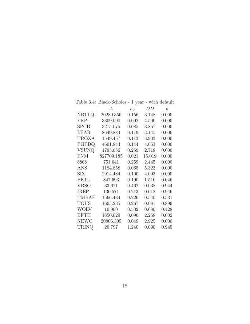
Table 3.4: Black-Scholes - 1 year - with default
A σA DD pNRTLQ 20289.350 0.156 3.148 0.000FRP 3309.090 0.092 4.506 0.000SPCB 3275.075 0.085 3.857 0.000LEAR 8649.884 0.119 3.145 0.000TROXA 1549.457 0.113 3.903 0.000PGPDQ 4601.844 0.144 4.053 0.000VSUNQ 1795.056 0.259 2.718 0.000FNM 827709.185 0.021 15.019 0.0008868 751.641 0.259 2.445 0.000ANS 1184.858 0.065 5.323 0.000SIX 2914.484 0.100 4.093 0.000PRTL 847.693 0.190 1.516 0.046VRSO 33.671 0.462 0.038 0.944IREP 130.571 0.213 0.012 0.946TMBAF 1566.434 0.226 0.540 0.531TOUS 1605.235 0.267 0.081 0.899WOLV 10.900 0.532 0.680 0.428BFTH 1650.029 0.096 2.268 0.002NEWC 20806.305 0.049 2.925 0.000TRINQ 20.797 1.240 0.090 0.945
18

Figure 3.2.2 compares this section model DD results with Moody’s data.Firms are ordered in descending order of DD (as computed by MKMV).
Figure 3.2: Moody’s vs BS-1Y-with default - distance to default
!"
#"
$"
%"
&"
'!"
'#"
'$"
'%"
()(*+"
,-."
/01-+"
&&%&"
-234+" 056
"4782"
32968" ,2
("8-0"
325-+
"
:94/"
-7:;"<,3="0(;<"(234"/209"527("
3.<8,"
3910"
!"#$%&
'()$*
)+(,%-
.$)
.>>?@AB" <0"C>?DE"F"'"@DGH"F"IJKL"?DMGNEK"
3.3 CEV Model
3.3.1 CEV Model - 1 year - without default
The results for this model are presented in Table 3.5.
19
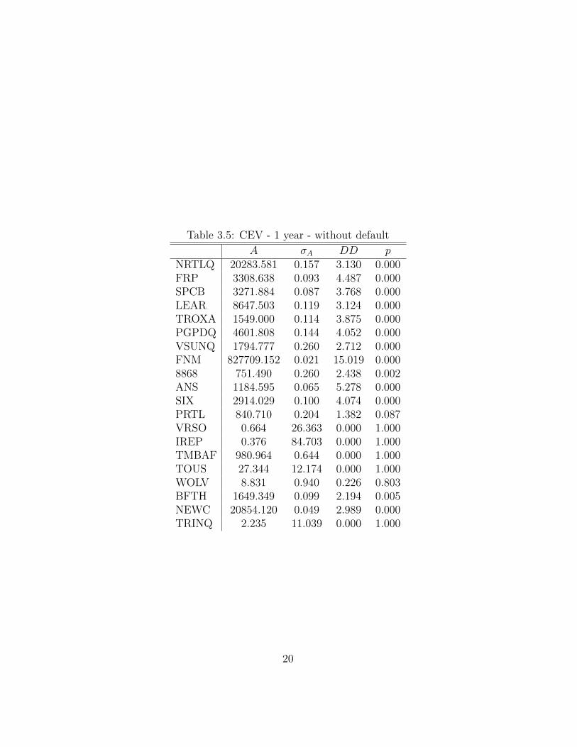
Table 3.5: CEV - 1 year - without default
A σA DD pNRTLQ 20283.581 0.157 3.130 0.000FRP 3308.638 0.093 4.487 0.000SPCB 3271.884 0.087 3.768 0.000LEAR 8647.503 0.119 3.124 0.000TROXA 1549.000 0.114 3.875 0.000PGPDQ 4601.808 0.144 4.052 0.000VSUNQ 1794.777 0.260 2.712 0.000FNM 827709.152 0.021 15.019 0.0008868 751.490 0.260 2.438 0.002ANS 1184.595 0.065 5.278 0.000SIX 2914.029 0.100 4.074 0.000PRTL 840.710 0.204 1.382 0.087VRSO 0.664 26.363 0.000 1.000IREP 0.376 84.703 0.000 1.000TMBAF 980.964 0.644 0.000 1.000TOUS 27.344 12.174 0.000 1.000WOLV 8.831 0.940 0.226 0.803BFTH 1649.349 0.099 2.194 0.005NEWC 20854.120 0.049 2.989 0.000TRINQ 2.235 11.039 0.000 1.000
20
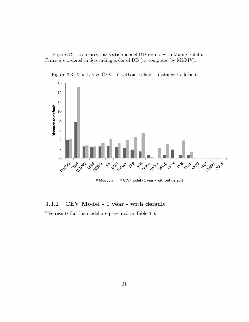
Figure 3.3.1 compares this section model DD results with Moody’s data.Firms are ordered in descending order of DD (as computed by MKMV).
Figure 3.3: Moody’s vs CEV-1Y-without default - distance to default
!"
#"
$"
%"
&"
'!"
'#"
'$"
'%"
()(*+"
,-."
/01-+"
&&%&"
-234+" 056
"4782"
32968" ,2
("8-0"
325-+
"
:94/"
-7:;"<,3="0(;<"(234"/209"527("
3.<8,"
3910"
!"#$%&
'()$*
)+(,%-
.$)
.>>?@AB" ;7/"C>?DE"F"'"@DGH"F"IJKL>MK"?DNGMEK"
3.3.2 CEV Model - 1 year - with default
The results for this model are presented in Table 3.6.
21
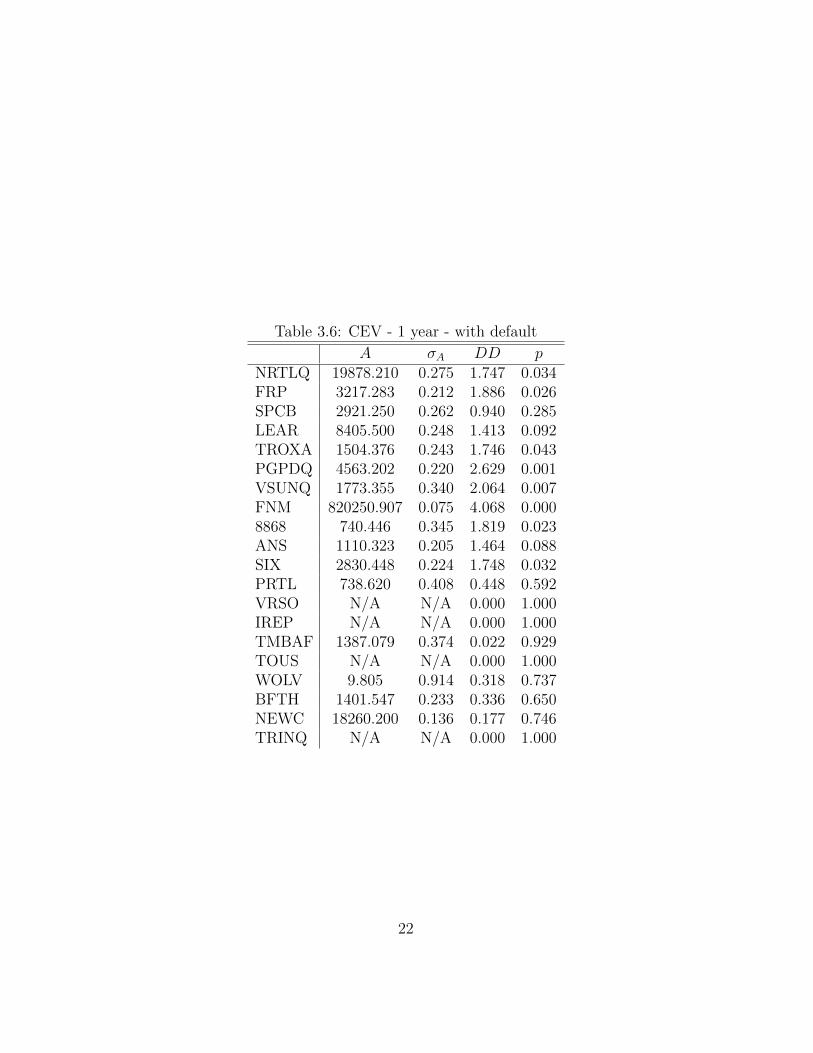
Table 3.6: CEV - 1 year - with default
A σA DD pNRTLQ 19878.210 0.275 1.747 0.034FRP 3217.283 0.212 1.886 0.026SPCB 2921.250 0.262 0.940 0.285LEAR 8405.500 0.248 1.413 0.092TROXA 1504.376 0.243 1.746 0.043PGPDQ 4563.202 0.220 2.629 0.001VSUNQ 1773.355 0.340 2.064 0.007FNM 820250.907 0.075 4.068 0.0008868 740.446 0.345 1.819 0.023ANS 1110.323 0.205 1.464 0.088SIX 2830.448 0.224 1.748 0.032PRTL 738.620 0.408 0.448 0.592VRSO N/A N/A 0.000 1.000IREP N/A N/A 0.000 1.000TMBAF 1387.079 0.374 0.022 0.929TOUS N/A N/A 0.000 1.000WOLV 9.805 0.914 0.318 0.737BFTH 1401.547 0.233 0.336 0.650NEWC 18260.200 0.136 0.177 0.746TRINQ N/A N/A 0.000 1.000
22

The equations used in this model weren’t able to provide estimates forthe values of A and σA of the firms VRSO, IREP, TMBAF and TRINQ. Thisparticularity of the model occurs for some firms with high EDF measures,for which equity is small relatively to total debt dp: when trying to solve thefirst equation of the System (2.12), we are faced with:
1. A positive drift for A;
2. A lower barrier for A, dp; if A is lesser than dp, ECEV (A, std, dp, r, τ)is automatically valued at 0;
3. An upper barrier for σA; since δA is uniquely determined by E and√E
trough the second equation of System (2.12), it is easy to see that σA
cannot be larger than δA√dp.
For some of the these firms, making A minimum (equal to dp) results in avalue for σA for which ECEV (A, std, dp, r, τ) is minimum but larger than E.
This behavior must not be considered a drawback of the model in ques-tion. We can interpret the results obtained by considering that, when nosolution is found, the market values observed imply that the firm is in factalready in default. As such, for these cases, we set DD = 0 and assign thefirm a probability of default equal to one. Figure 3.3.2 compares this sec-tion model DD results with Moody’s data. As before, firms are ordered indescending order of DD (as computed by MKMV).
23

Figure 3.4: Moody’s vs CEV-1Y-with default - distance to default
!"
#"
$"
%"
&"
'"
("
)"
*"
+"
,-,./"
012"
3451/"
**(*"
1678/" 49:
"
8;<6"
76=:<"
06,"
<14"
7691/"
>=83"
1;>?"
@07A"
4,?@"
,678"
364="96;,"
72@<0"
7=54"
!"#$%&
'()$*
)+(,%-
.$)
2BBCDEF" ?;3"GBCHI"J"#"DHKL"J"MNOP"CHQKRIO"
24
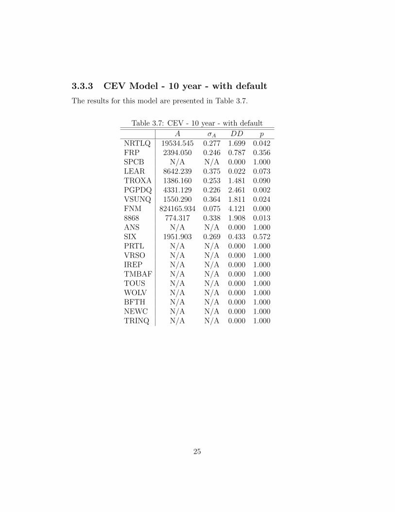
3.3.3 CEV Model - 10 year - with default
The results for this model are presented in Table 3.7.
Table 3.7: CEV - 10 year - with default
A σA DD pNRTLQ 19534.545 0.277 1.699 0.042FRP 2394.050 0.246 0.787 0.356SPCB N/A N/A 0.000 1.000LEAR 8642.239 0.375 0.022 0.073TROXA 1386.160 0.253 1.481 0.090PGPDQ 4331.129 0.226 2.461 0.002VSUNQ 1550.290 0.364 1.811 0.024FNM 824165.934 0.075 4.121 0.0008868 774.317 0.338 1.908 0.013ANS N/A N/A 0.000 1.000SIX 1951.903 0.269 0.433 0.572PRTL N/A N/A 0.000 1.000VRSO N/A N/A 0.000 1.000IREP N/A N/A 0.000 1.000TMBAF N/A N/A 0.000 1.000TOUS N/A N/A 0.000 1.000WOLV N/A N/A 0.000 1.000BFTH N/A N/A 0.000 1.000NEWC N/A N/A 0.000 1.000TRINQ N/A N/A 0.000 1.000
25
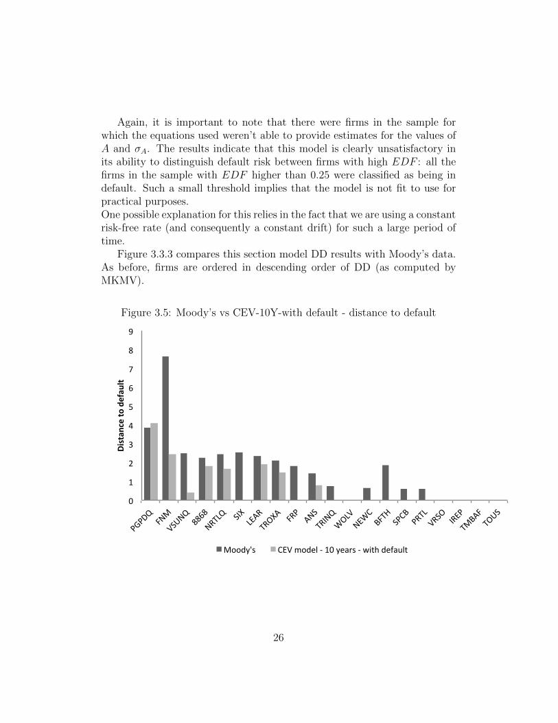
Again, it is important to note that there were firms in the sample forwhich the equations used weren’t able to provide estimates for the values ofA and σA. The results indicate that this model is clearly unsatisfactory inits ability to distinguish default risk between firms with high EDF : all thefirms in the sample with EDF higher than 0.25 were classified as being indefault. Such a small threshold implies that the model is not fit to use forpractical purposes.One possible explanation for this relies in the fact that we are using a constantrisk-free rate (and consequently a constant drift) for such a large period oftime.
Figure 3.3.3 compares this section model DD results with Moody’s data.As before, firms are ordered in descending order of DD (as computed byMKMV).
Figure 3.5: Moody’s vs CEV-10Y-with default - distance to default
!"
#"
$"
%"
&"
'"
("
)"
*"
+"
,-,./"
012"
3451/"
**(*"
1678/" 49:
"
8;<6"
76=:<"
06,"
<14"
7691/"
>=83"
1;>?"
@07A"
4,?@"
,678"
364="96;,"
72@<0"
7=54"
!"#$%&
'()$*
)+(,%-
.$)
2BBCDEF" ?;3"GBCHI"J"#!"DHKLF"J"MNOP"CHQKRIO"
26

3.4 Comparison of the Models
Table 3.8 compares the results obtained in terms of:
1. Sample mean of the difference between MKVM DD values and each ofthe other method’s DD values (DD), computed by the formula:
DD =
�20i=1 |DDMi −DDmi|
20,
where DDMi and DDmi denote, respectively, the DD value suppliedby MKVM for firm i of the sample and the DD value obtained for firmi from the model to which we are applying the formula.
2. Sample mean of the difference between MKVM default probability val-ues and each of the other method’s default probabilities (p), which isobtained trough the use of the expression:
p =
�20i=1 |pMi − pmi|
20,
where pMi denotes the one-year default probability estimated by MKVMfor firm i of the sample and pmi denotes the the same default proba-bility for firm i but obtained from the model to which we are applyingthe formula 1.
Table 3.8: Models Comparisons
DD pBS - 1Y - no default 1.5148 0.0691BS - 1Y - default 1.5239 0.0691CEV - 1Y - no default 1.5027 0.0668CEV - 1Y - default 0.6073 0.0450CEV - 10Y- default 0.4920 0.0939
In general, the models proposed seem to provide poor results.
1MKVM truncates its EDF measures at 35%, so for each default probabilities estimatedby our models that are larger than 0.35, we replace them with 0.35 in these computations.
27

BothDD and p are estimators of, respectively, the absolute difference be-tween our model’s DD values and MKMV values and the absolute differencebetween our model’s default probabilities and MKMV EDF values.
Therefore, a value for DD close to 1.5, as was obtained in three of theproposed models, implies that we should expect, on average, to commit anan absolute error of 1.5. This seems substantially high when compared to theDD values in our sample (note that changing a DD value by 1.5 in any of thefirms would immediately lead us to consider her substantially riskier/saferthan many other firms in the sample). Similarly, an error of approximately600 basis points (or even 450), makes it implausible to use this models for,say, CDS pricing.
Surprisingly, the model described in section 3.3.2 provides much betterresults than the remaining ones and seems to be the best alternative toestimate Moody’s KMV Distance to Default. It’s DD is half of the valueobtained with the models from the first three sections. It possesses the secondsmallest DD and smallest p.
28

Chapter 4
Conclusion
The approach followed in this thesis resulted in models that exhibited a toomuch poor performance for them to be used in practice as methods for theestimation of Moody’s KMV Distance to Default.
Nevertheless, one of the proposed methods showed substantially betterresults than the remaining ones, and in particular showed better results thanthe methods based on the Black-Scholes model. This implies that it shouldbe in no way excluded the possibility of obtaining different structural modelsbetter fit to estimate MKVM DD.
The model who exhibited better results was based on interpreting equityas one-year Down and Out Call Option on the firm’s assets who were deter-mined to follow a CEV Square Model and on postulating directly a functionalrelation between the firm’s asset’s volatility and equity volatility. This in-volved the use of Monte Carlo methods in order to evaluate Down and OutCall Options.
29
Appendix A
Auxiliary Results
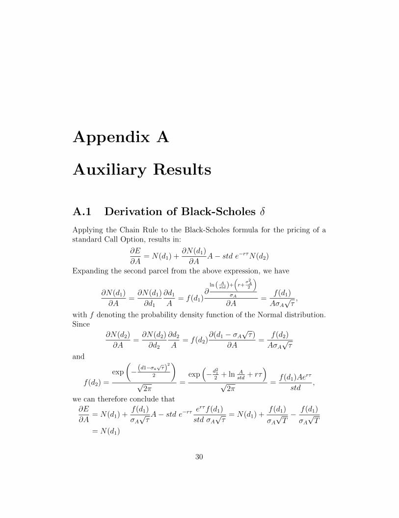
A.1 Derivation of Black-Scholes δ
Applying the Chain Rule to the Black-Scholes formula for the pricing of astandard Call Option, results in:
∂E
∂A= N(d1) +
∂N(d1)
∂AA− std e−rτN(d2)
Expanding the second parcel from the above expression, we have
∂N(d1)
∂A=
∂N(d1)
∂d1
∂d1A
= f(d1)∂
ln ( Astd)+
�r+
σ2A2
�
σA
∂A=
f(d1)
AσA√τ,
with f denoting the probability density function of the Normal distribution.Since
∂N(d2)
∂A=
∂N(d2)
∂d2
∂d2A
= f(d2)∂(d1 − σA
√τ)
∂A=
f(d2)
AσA√τ
and
f(d2) =
exp
�−(d1−σa
√τ)
2
2
�
√2π
=exp
�−d21
2 + ln Astd + rτ
�
√2π
=f(d1)Aerτ
std,
we can therefore conclude that∂E
∂A= N(d1) +
f(d1)
σA√τA− std e−rτ erτf(d1)
std σA√τ= N(d1) +
f(d1)
σA
√T
− f(d1)
σA
√T
= N(d1)
30

Appendix B
Auxiliary Tables
B.1 Firms used in the sample
31
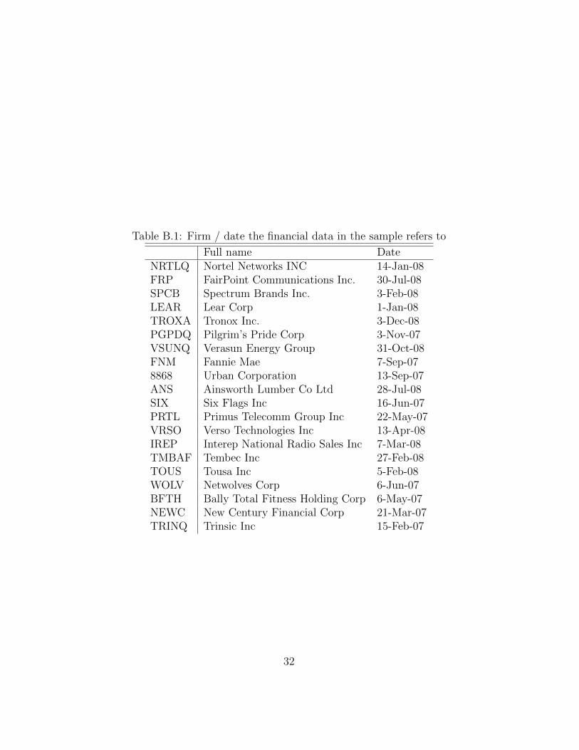
Table B.1: Firm / date the financial data in the sample refers to
Full name DateNRTLQ Nortel Networks INC 14-Jan-08FRP FairPoint Communications Inc. 30-Jul-08SPCB Spectrum Brands Inc. 3-Feb-08LEAR Lear Corp 1-Jan-08TROXA Tronox Inc. 3-Dec-08PGPDQ Pilgrim’s Pride Corp 3-Nov-07VSUNQ Verasun Energy Group 31-Oct-08FNM Fannie Mae 7-Sep-078868 Urban Corporation 13-Sep-07ANS Ainsworth Lumber Co Ltd 28-Jul-08SIX Six Flags Inc 16-Jun-07PRTL Primus Telecomm Group Inc 22-May-07VRSO Verso Technologies Inc 13-Apr-08IREP Interep National Radio Sales Inc 7-Mar-08TMBAF Tembec Inc 27-Feb-08TOUS Tousa Inc 5-Feb-08WOLV Netwolves Corp 6-Jun-07BFTH Bally Total Fitness Holding Corp 6-May-07NEWC New Century Financial Corp 21-Mar-07TRINQ Trinsic Inc 15-Feb-07
32

Appendix C
Monte Carlo Methods
C.1 ECEV (A,X, dp, r, τ )
The steps we follow to compute ECEV (A,X, dp, r, τ) are:
1. Determine a number of sample paths ite and number of points per pathn to be used. In our case, we defined ite = 1000 and n = 10.
2. Generate ite sample paths with n points, using the distribution spec-ified for A. This is possible when, as is the case, the distribution ofAt|A0=A is known, by following the steps:
i. Generate a pseudo-random number (rand) between 0 and 1;
ii. Solve the equation FA 1n|A0=A
= rand to generate the path’s next
point;
iii. Repeat the previous two steps, replacing the initial value for Awith the last step’s result;
iv. Stop when A1 is determined.
3. For each path generated, determine its minimum. If it is less than dp,replace the path’s endpoint by X + 1.
4. Replace each path’s endpoint (ep) with the value max(X − ep, 0).
5. Sum all the endpoints of all paths and divide the result by ite. Thevalue obtained is an estimate for the terminal payoff of our call.
6. Multiply the previous result by e−r to determine its present value.
33

C.2 ECEV10(A, std, ltd, dp, r, τ )
The steps we follow to compute ECEV10(A, std, ltd, dp, r, τ) are:
1. Determine a number of sample paths ite and number of points per pathn to be used. In our case, we defined ite = 1000 and n = 12.
2. Generate ite sample paths with n points, using the distribution spec-ified for A. This is possible when, as is the case, the distribution ofAt|A0=A is known, by following the steps:
i. Generate a pseudo-random number (rand) between 0 and 1;
ii. Solve the equation FA 1n|A0=A
= rand to generate the path’s next
point;
iii. Repeat the previous two steps, replacing the initial value for Awith the last step’s result;
iv. Stop when A1 is determined;
v. If our path’s current minimum point is less than dp, set the currentpath’s endpoint (ep) equal to 0 and start generating a new path.Otherwise, set A = (A− std) and dp = (dp− std) and return to iii;
vi. Stop when A10 is determined.
3. For each path generated, determine its minimum. If it is less than dp,replace the path’s endpoint by X + 1.
4. Replace each path’s endpoint (ep) with the value max(X − ep, 0).
5. Sum all the endpoints of all paths and divide the result by ite. Thevalue obtained is an estimate for the terminal payoff of our call.
6. Multiply the previous result by e−r to determine its present value.
34

Bibliography
Navneet Arora, Jeffrey Bohn, and Fanlin Zhu. Reduced Form Vs. Struc-tural Models of Credit Risk: a Case Study of Three Models. Journal ofInvestment Management, 3(4):43–67, 2005.
Stan Beckers. The Constant Elasticity of Variance Model and Its Implicationsfor Option Pricing. Journal of Finance, 35:661–673, 1980.
Fischer Black and Myron Scholes. The Pricing of Options and CorporateLiabilities. Journal of Political Economy, 81(3):637–654, 1973.
Andrew Christie. The Stochastic Behavior of Common Stock Variances.Journal of Financial Economics, 10:407–432, 1982.
John Cox. Notes on Option Pricing I: Constant Elasticity of Variance Diffu-sions. Standford University, 1975.
Peter Crosbie and Jeff Bohn. Modeling Default Risk. Moody’s KMV Com-pany, 2003.
Douglas Dwyer and Shisheng Qu. EDF 8.0 Model Enhancements. Moody’sKMV Company, 2007.
Robert Merton. Theory of Rational Option Pricing. The Bell Journal ofEconomics and Management Science, 4(1):141–183, 1973.
Robert Merton. On the Pricing of Corporate Debt: The Risk Structure ofInterest Rates. Journal of Finance, 28:449–470, 1974.
Oldrich Alfons Vasicek. Credit Valuation. KMV Company, 1984.
35