guidelines for operating congested traffic signals · guidelines for operating congested traffic...
TRANSCRIPT

Technical Report Documentation Page 1. Report No. FHWA/TX-10/0-5998-1
2. Government Accession No.
3. Recipient's Catalog No.
4. Title and Subtitle GUIDELINES FOR OPERATING CONGESTED TRAFFIC SIGNALS
5. Report Date December 2009 Published: August 2010 6. Performing Organization Code
7. Author(s) Nadeem A. Chaudhary, Chi-Leung Chu, Srinivasa R. Sunkari, and Kevin N. Balke
8. Performing Organization Report No. Report 0-5998-1
9. Performing Organization Name and Address Texas Transportation Institute The Texas A&M University System College Station, Texas 77843-3135
10. Work Unit No. (TRAIS) 11. Contract or Grant No. Project 0-5998
12. Sponsoring Agency Name and Address Texas Department of Transportation Research and Technology Implementation Office P.O. Box 5080 Austin, Texas 78763-5080
13. Type of Report and Period Covered Technical Report: September 2007–August 2009 14. Sponsoring Agency Code
15. Supplementary Notes Project performed in cooperation with the Texas Department of Transportation and the Federal Highway Administration. Project Title: Evaluation of Best Practices for Controlling Signal Systems during Oversaturated Conditions URL: http://tti.tamu.edu/documents/0-5998-1.pdf 16. Abstract The objective of this project was to develop guidelines for mitigating congestion in traffic signal systems. As part of the project, researchers conducted a thorough review of literature and developed preliminary guidelines for combating congestion. Then, the researchers conducted a survey of selected practitioners in Texas to get feedback on their concerns about congestion and opinions about a list of strategies developed after literature review. Researchers also conducted simulation studies to analyze the impact of bay length, traffic distribution, and phasing sequence selection on the throughput capacity of left-turn bay and adjacent through lane under loaded traffic conditions. Researchers also conducted field and simulation studies to show the applications of preliminary guidelines. Finally, they modified guidelines to account for lessons learned through field studies. 17. Key Words Traffic Signals, Traffic Congestion, Guidelines, Queue Management, Traffic Simulation
18. Distribution Statement No restrictions. This document is available to the public through NTIS: National Technical Information Service Springfield, Virginia 22161 http://www.ntis.gov
19. Security Classif.(of this report) Unclassified
20. Security Classif.(of this page) Unclassified
21. No. of Pages 120
22. Price
Form DOT F 1700.7 (8-72) Reproduction of completed page authorized


GUIDELINES FOR OPERATING CONGESTED TRAFFIC SIGNALS
by
Nadeem A. Chaudhary, Ph.D., P.E. Senior Research Engineer
Texas Transportation Institute
Chi-Leung Chu, Ph.D. Associate Transportation Researcher
Texas Transportation Institute
Srinivasa R. Sunkari, P.E. Research Engineer
Texas Transportation Institute
and
Kevin N. Balke, Ph.D., P.E. Center Director, TransLink® Research Center
Texas Transportation Institute
Report 0-5998-1 Project 0-5998
Project Title: Evaluation of Best Practices for Controlling Signal Systems during Oversaturated Conditions
Performed in cooperation with the Texas Department of Transportation
and the Federal Highway Administration
December 2009 Published: August 2010
TEXAS TRANSPORTATION INSTITUTE The Texas A&M University System College Station, Texas 77843-3135


v
DISCLAIMER
This research was performed in cooperation with the Texas Department of Transportation (TxDOT) and the Federal Highway Administration (FHWA). The contents of this report reflect the views of the authors, who are responsible for the facts and the accuracy of the data presented herein. The contents do not necessarily reflect the official view or policies of the FHWA or TxDOT. This report does not constitute a standard, specification, or regulation. This report is not intended for construction, bidding, or permit purposes. The engineer in charge of the project was Nadeem A. Chaudhary, P.E. #66470.
vi
ACKNOWLEDGMENTS
This project was conducted in cooperation with TxDOT and FHWA. Authors would like to acknowledge guidance and support received from the project director Mr. Henry Wickes and members of the Project Monitoring Committee. These individuals included Mr. Adam Chodkiewics, Mr. Don Baker, Mr. David Danz, Mr. Derryl Skinnell and Mr. Gordon Harkey. Authors would also like to acknowledge support provided by RTI staff Ms. Loretta Brown and Mr. Wade Odell. Special thanks go to Mr. Ali Mozdbar, City of Austin, and Mr. Pat Walker, City of College Station, for their support with data collection and implementation of timings. Authors also acknowledge assistance in data collection provided by Dr. Geza Pesti of the Texas Transportation Institute.

vii
TABLE OF CONTENTS
Page List of Figures ............................................................................................................................. viii List of Tables ................................................................................................................................ ix Chapter 1. Introduction................................................................................................................ 1
Background ................................................................................................................................. 1 Literature Review........................................................................................................................ 2
Chapter 2. State of Practice in Texas .......................................................................................... 7 Chapter 3. Preliminary Congestion Management Guidelines .................................................. 9
Characteristics and Causes of Traffic Congestion ...................................................................... 9 Congestion Management Guidelines ........................................................................................ 13
Chapter 4. Impact of Left-Turn Bay on Signal Capacity ....................................................... 17 Single-Lane Left-Turn Bay Case .............................................................................................. 17
Design of Experiment ........................................................................................................... 17 Fixed-Time Control .............................................................................................................. 19 Fully-Actuated Control ......................................................................................................... 23
Simulation Experiments for Dual Left-Turn Bay ..................................................................... 26 Simulation Experiments Using Timings for the Single-Lane Case ...................................... 26 Simulation Experiment with Revised Timings ..................................................................... 27
Throughput Capacity Estimation Example ............................................................................... 29 Conclusions ............................................................................................................................... 30
Chapter 5. Applications to Real Problems ............................................................................... 33 Three-Intersection System in College Station .......................................................................... 33
Application of General Congestion Management Guidelines .............................................. 34 Signalized Intersection in Austin .............................................................................................. 45
Application of General Congestion Management Guidelines .............................................. 45 Challenges ................................................................................................................................. 52
Chapter 6. Revised Congestion Mitigation Guidelines ............................................................ 55 References .................................................................................................................................... 59 Appendix A. Questionnaire ........................................................................................................ 63 Appendix B. Summary of Responses to Questionnaire ........................................................... 73 Appendix C. Simulation Results for the Fixed-Time Control Scenario ................................ 83 Appendix D. Simulation Results for the Fully-Actuated Control Scenario .......................... 89 Appendix E. Simulation Results for Dual Left-Turn Bay with Fixed-Time Control and
Previous Timings .............................................................................................. 95 Appendix F. Percent Demand Served for Selected Cases of Single Left-Turn Lane with
Fixed-Time Traffic Signal ............................................................................. 101 Appendix G. Simulation Results for Dual Left-Turn Bay with Fixed-Time Control and
Retimed Signal ............................................................................................... 105

viii
LIST OF FIGURES
Page Figure 1. Cumulative Flows of a Signalized Intersection. .............................................................. 9 Figure 2. Effect of Cycle Length on Cycle-by-Cycle Queue Length. .......................................... 10 Figure 3. Examples of Best and Worst Signal Coordination. ....................................................... 11 Figure 4. Congestion Caused by Suboptimal Signal Timings. ..................................................... 11 Figure 5. Spillback and Starvation Caused by a Short Left-Turn Bay. ........................................ 12 Figure 6. Wide-Spread Congestion. .............................................................................................. 12 Figure 7. Results Produced by a Reduced Cycle Length and Non-Orthodox Green Splits. ......... 13 Figure 8. General Congestion Management Guidelines. .............................................................. 13 Figure 9. Geometric Layout of the Isolated Intersection Studied. ................................................ 17 Figure 10. Eastbound Productivity for 100-ft Bay and 100-second Cycle Length. ...................... 19 Figure 11. Eastbound Productivity for 300-ft Bay and 100-second Cycle Length. ...................... 20 Figure 12. Eastbound Productivity for 500-ft Bay and 100-second Cycle Length. ...................... 20 Figure 13. Productivity of Restricted Approach versus Cycle Length. ........................................ 21 Figure 14. Approach Productivity for 90-second Cycle Length and Different Bay Lengths. ...... 22 Figure 15. Approach Productivity for 110-second Cycle Length and Different Bay Lengths. .... 22 Figure 16. Approach Productivity for 130-second Cycle Length and Different Bay Lengths. .... 23 Figure 17. Layout of Stopbar Detector for Fully-Actuated Control. ............................................ 24 Figure 18. Productivity of Restricted Approach Volume Scenarios under Fully-Actuated
Control. ................................................................................................................. 24 Figure 19. Phasing Sequence Example for Fully-Actuated Control. ............................................ 25 Figure 20. Geometric Layout for Dual Left-Turn Bay Experiments. ........................................... 27 Figure 21. Geometric Layout with Dual Left-Turn Lanes. ........................................................... 28 Figure 22. Geometric Layout of the Example. ............................................................................. 29 Figure 23. Three-Intersection System at George Bush Drive in College Station, Texas. ............ 33 Figure 24. Video Capture of Olsen Boulevard at George Bush Drive. ........................................ 36 Figure 25. Video Capture of Marion Pugh Drive at George Bush Drive. .................................... 36 Figure 26. Video Capture of Wellborn Road at George Bush Drive. ........................................... 37 Figure 27. Screenshot of VISSIM Model of the College Station Site. ......................................... 38 Figure 28. Phase Numbering at Olsen Boulevard and George Bush Drive Intersection. ............. 39 Figure 29. Performance Analysis for Wellborn Road and George Bush Drive Intersection. ....... 40 Figure 30. Performance Analysis for Olsen Boulevard and George Bush Drive Intersection. .... 41 Figure 31. Signalized Intersection at US 360 in Austin, Texas. ................................................... 46 Figure 32. Camera Location and View Direction at US 360, Austin, Texas. ............................... 47 Figure 33. Screenshot of View A. ................................................................................................. 47 Figure 34. Screenshot of View B. ................................................................................................. 48 Figure 35. Screenshot of View C. ................................................................................................. 48 Figure 36. Cumulative Distribution of Headways for Southbound Traffic. ................................. 50 Figure 37. Cumulative Distribution of Headways for Northbound Traffic. ................................. 50 Figure 38. Routing Decision in VISSIM. ..................................................................................... 54 Figure 39. General Congestion Management Guidelines. ............................................................ 55

ix
LIST OF TABLES
Page Table 1. Responses to Questionnaire. ............................................................................................. 7 Table 2. Simulation Scenario Matrix. ........................................................................................... 18 Table 3. Capacity Data Obtained Using HCM Method. ............................................................... 29 Table 4. Results of the Cycle Length Search Process. .................................................................. 42 Table 5. Maximum and Average Queue Lengths in Feet. ............................................................ 43 Table 6. Maximum and Average Queue Lengths of the Proposed Timing Plan. ......................... 43 Table 7. Proposed Max Time Settings for College Station Site. .................................................. 43 Table 8. Results of the Cycle Length Search Process if Equipment Is Fixed. .............................. 44 Table 9. Estimated Capacities of the Proposed Timing Plan. ....................................................... 51 Table 10. Queue Dissipation Estimation. ..................................................................................... 52


1
CHAPTER 1. INTRODUCTION
BACKGROUND
In recent years, there has been a sharp increase in the number of metropolitan areas facing severe traffic congestion in their signalized systems. Furthermore, the severity of traffic congestion on signalized roadways has continued to increase at a steady pace, resulting in longer periods of congestion. A recent study conducted by National Transportation Operations Coalition to assess the health of nation’s signal system estimated that poor signal timing accounts for 5–10 percent of all traffic delays (1). This study gave a score of D to overall signal operations in the United States. Citing previous findings that the benefits-to-cost ratio of signal retiming is 40:1 or better, this study recommended routine timing updates to improve the current low grade. This simple recommendation is easier said than done when dealing with congested traffic signals.
At the 2006 summer meeting of Transportation Research Board’s (TRB) Signal Systems committee, a panel of experts identified several factors that prevent effective management of congested traffic signals. These factors include:
• a lack of consistent definitions for oversaturation and congestion as they pertain to traffic signals and signal systems,
• absence of procedures and guidelines for correctly assessing traffic demand, • a lack of guidelines for characterization of congestion, identifying its causes, and
assessments of its impacts, • a lack of guidelines for selection of appropriate control objectives, and • a lack of systematic procedures and tools for deriving appropriate signal control plans.
The TRB panel agreed to proactively push a research agenda specifically geared toward
improving tools and technology for operating congested traffic signals. The panel further agreed that the first research step should focus on the identification and documentation of:
1. the state of technology and its deficiencies, 2. the types and causes of common congestion problems in signal systems, and 3. the current state of practice to deal with identified problems.
The next step would be to develop guidelines for improving common types of congestion
problems at traffic signals using existing technology and lessons learned from successes and failures in the field. To facilitate the first step, TRB Signal Systems Committee sponsored a special workshop on the topic of congested signals. This workshop, organized by two members of the Texas Transportation Institute (TTI) team assembled for this project, was held during the January 2007 Annual TRB meeting in Washington, D.C. At the national level, this effort resulted in a Federal Highway Administration project, whose focus was to develop guidelines for individual signalized intersections facing congested conditions. About the same time, TxDOT initiated this project, but with a broader focus, which includes signal systems. The primary objectives of this project were to:
2
1. Assess state of traffic signal control technology and its limitations as it pertains to congested traffic signals.
2. Identify state-of-practice in Texas as it pertains to understanding of the congestion problems, its consequences, and feasible strategies to cope with it.
3. Use information gained from the reviews of available technology and current practices to develop preliminary guidelines for improving traffic flow at congested signals.
4. Use results from computer simulations and field studies to refine the preliminary guidelines.
LITERATURE REVIEW
Signal optimization for congested conditions has been studied since the 1960s. In 1963, Gazis and Potts (2) proposed a “store and forward” strategy for dealing with oversaturated traffic signals. This strategy, refined and presented later (3), uses time varying traffic demands combined with a mathematical programming approach to optimally store and dissipate queues at signals where demand exceeds capacity. This store and forward approach does not account for the effects of queue variation within a cycle and offsets. Rahmann (4) argued that queuing would be a norm during peak periods and presented the idea of designing signals as storage/output devices, even during undersaturated conditions. Pignataro et al. (5) attempted to define congestion and oversaturation in terms of their causes and scope, and proposed guidelines for dealing with such conditions. They proposed three solutions: (1) minimal-response signal policies (i.e., cycle length selection matched to block length), (2) highly responsive signal policies (i.e., queue actuated control [6]), and (3) other non-signal treatments (i.e., enforcement and prohibiting, right-turn-on-red) in a signalized environment. As reported by Lee et al. (6), the primary objective of the queue-control policy was to delay or eliminate intersection blockage. Lieberman and Messer (7) developed mathematical models for optimizing signal timings based on an internal metering policy. Internal metering ensures that no link receives more traffic than it can hold without spilling back traffic, requiring the determination of best green splits and offsets. The objective of such models is to maximize throughput. Other researchers have continued to refine these ideas. For instance, Gal-Tzur et al. (8) developed an iterative signal-timing optimization method, which linked a custom mathematical program with TRANSYT signal-timing optimization program. In this scheme, the mathematical model was used to determine the green splits and the level of metering, whereas TRANSYT was used for simulating the dynamic processes within the cycle and for offset optimization. Other instances include the works of Choi (9) and Lieberman and Chang (10) who refined the internal metering models and demonstrated their real-time application. Kim (11) and Kim and Messer (12) developed mathematical models for controlling congested interchanges and arterials with single critical intersections. These models managed queues at external approaches to a system, while preventing spillback and reducing delay on the interior links.
Research conducted by Chaudhary and Balke (13) found that driver expectancy plays an important role in determining headways and those variations in headways increase for vehicles further back in the queue. The implication of this finding is that capacity may be lost if very long cycles are used. They studied five coordination strategies using computer simulation. The results of this study showed that coordination of actuated signals for progressing traffic flow in the congested direction produces lower delays, fewer stops, and shorter queues. In his work with

3
congested interchanges, Messer (14) found that undersaturated systems might become congested because of poor signal timing and deficient spacing between the signalized intersections. By providing an upper bound on signal control delay for oversaturated arterial operations, he showed that congestion can be characterized and modeled. Messer (15) extended an existing model for analyzing the operational impacts of queue spillback on the capacity and delay of closely spaced signalized intersections. Chaudhary and Chu (16) and Chaudhary et al. (17) developed two models for coordinating diamond interchanges with adjacent signals. Their first model is a simple capacity analysis procedure that uses Webster’s method (18) for calculating green splits for the interchange and adjacent signals. However, Webster’s green split calculation method, which treats each signalized intersection separately, may not be valid when queues from one intersection start to influence an adjacent signal. To accommodate such situations, the second model uses an iterative method for simultaneously calculating green splits and offsets for all signals in the system. The procedure automatically determines if the system is undersaturated or oversaturated. If the system is oversaturated, it pushes all excess demand to the user-defined boundary of the system, while keeping the interior links clear of detrimental queues (19). Although this method needs refinements, it has shown to produce excellent results for small systems.
Other researchers have continued to explore the development of methods and models to deal with congested traffic signal systems. Abu-Lebdeh and Benekohal (20) developed a model for maximizing system throughput by managing queues. Liu and Masao (21) developed a model based on the method of cumulative flows. The objective of this model is to minimize delay by allocating green times to various phases. Ahn and Machemehl (22) developed a traffic simulation model to provide a methodology for traffic signal timing in oversaturated urban arterial networks. They considered two control objectives: maximizing throughput and preventing or minimizing queue spillback. They found that offset was a dominating factor. Other factors found to be important were link length and cross street green time. Abu-Lebdeh and Benekohal (23) developed models for estimating the capacities of oversaturated arterials. Khatib et al. (24) propose that the goal of timing in congested conditions should be to allow higher-volume approaches to discharge more traffic than the lower-volume approaches, so that the intersection can return to a normal condition as quickly as possible. They developed and simulation-tested mathematical models that optimize maximum green intervals for achieving this goal by preventing spillback and overflow on signalized arterials with actuated signals. Girianna and Benekohal (25) developed an algorithm that determines green times and offsets to manage/distribute queues in time and space.
Herrick and Messer (26) developed guidelines and strategies for improving traffic operations at signalized diamond interchanges that become oversaturated for periods of time and recommended enhanced features for third-generation traffic control, including enhanced traffic detector strategies to identify the presence of queue backups onto the freeway during oversaturated conditions.
A recently completed FHWA project (27) has developed guidelines and proposed
strategies to mitigate the effects congestions have at isolated signalized intersections using input from a panel of seven experts, limited computer simulation, and one field study at a three-legged severely-congested intersection in Virginia. Depending on the situation, some of the proposed

4
strategies may or may not be feasible. Furthermore, the FHWA report does not offer practical steps for their implementation.
While researchers continue their quest for improved congestion management strategies and models, practitioners must continue attempt to solve their problems using whatever means available to them. The literature provides a glimpse of such attempts, including:
• a trial and error method, which kept shifting congestion from one location in the system to another (28);
• after failing to mitigate severe congestion on a 2.72-mile arterial stretch via optimization of signal timing parameters, resorting to a flush strategy that ignored cross streets (29);
• successful development of a strategy to improve congestion and safety in a small corridor, but failure in implementation due to inter-jurisdictional barriers (30);
• success by fixing downstream problems, using appropriate cycle length, double-servicing heavy phases, running closely-spaced signals using a single controller, and doing whatever it takes to coordinate all closely-spaced intersections with the problematic signal (31); and
• success by using flexible timing, efficient placement of detectors, queue detection, efficient gap settings to minimize duration of oversaturation, variable walk time, and use of other advanced controller features (32).
Coordinating signals to alleviate the adverse effects of traffic congestion is the fastest and
the least costly approach, but it may not cure severe congestion. When that happens, other more expansive approaches are warranted to increase or add capacity. These approaches include: adding lanes, changing intersection geometry, extending turn bays, restricting on-street parking, converting two-way streets to one-way streets, using reversible lanes (33), and grade separation. Access management is another capacity-improvement strategy. Identifying access management as a response to the problems of congestions, capacity loss, and accidents along roadway, Koepke and Levinson (34) provide access management guidelines for activity centers. Gluck et al. (35) reviewed different access management techniques and discussed corresponding safety and operations. An example of access management is the Michigan left-turn, which replaced an at-intersection left-turn movement with a right- plus U-turn movement. The advantages of this treatment include reduction in delay, increased intersection capacity, better progression for through traffic, fewer stops for through traffic, and fewer conflict points (36) in the intersection. Gluck et al. (35) cited the results of Koepke and Levinson in which the estimated capacity gains of Michigan left-turn over dual left-turn lanes range from 14 percent to 18 percent and the estimated reduction in critical lane volumes ranges from 7 percent to 10 percent.
Another approach to combat congestion is to manage demand. Approaches in this category include encouraging employers to implement staggered and/or flexible working hours, encouraging car pooling by providing toll discounts and/or high occupancy lanes, encouraging the use of transit services by providing conveniently-accessible park-and-ride lots, discouraging trips by increasing parking rates, and tolling (33).
Though congestion is one of the major issues faced by many metropolitan areas, there
exists no standard agreed-upon measure for characterizing its severity. While throughput, extent

5
of queuing, and delay are useful in characterizing congestion and identifying its consequences, they alone do not provide solution strategies. Gazis and Potts (2) classified congestion into four categories. However, this classification lacks an objective measure. Lindley (37) developed the congestion severity index that is based on delay. Levinson and Lomax (38) proposed using a delay rate index as a measure for congestion, where delay rate is the difference between per-minute delays under free-flow and congested conditions. By conducting an opinion survey with a group of traffic experts and users, Vaziri (39) developed a congestion index using fuzzy set theory. By considering average travel speed and the proportion of time traveling at very low speed within the total travel time, Hamad and Kikuchi (40) proposed a traffic congestion index with values is the range of 0 to 1, where 0 indicates the best condition and 1 indicates the worst condition. Even though research efforts on developing a congestion index are continuing, its use is not widely accepted partly because congestion is not a well defined condition. In addition, the effectiveness of the use of such index in congestion mitigation strategies requires further investigation.


7
CHAPTER 2. STATE OF PRACTICE IN TEXAS
To identify the state of practice regarding oversaturated condition in Texas, researchers developed a questionnaire for soliciting information from practitioners in Texas. This questionnaire is reproduced in Appendix A. In consultation with the TxDOT advisory panel, researchers concluded that it would be sufficient to solicit information from a carefully-selected group of experts consisting of TxDOT employees, other public agencies, and consultants.
In May 2008, the questionnaire was sent to 27 selected individuals. Table 1 provides a summary of responses received.
Table 1. Responses to Questionnaire.
Agency Sent Received % Returned TxDOT 12 9 75.0 Other Public Agency 8 6 75.0 Consultant 7 2 28.6 Total 27 17 62.9
As can be seen from this table, the response from TxDOT and other public agency staff was excellent (75 percent returns each). Most individuals in these agencies returned the completed surveys by the end of June. Only two out of seven responses were received from consultants. Appendix B provides a summary of survey results. The following are key findings from the survey of practitioners in Texas:
• Congestion was identified to occur mostly in coordinated systems. Key characteristics of congestion identified were:
o two to three consecutive cycles failures at an approach; o capacity loss due to queue spillback and blocking; o long queues on one or more approaches. These queues may be local or from
adjacent intersections; and o inability to provide acceptable progression.
• Key objectives for tackling congestion at isolated intersections were identified to be:
o minimizing delay, o maximizing throughput, o providing equity to movements at an intersection, and o minimizing cycles required to go through an approach.
• Key objectives for tackling congestion in signal systems were identified to be: o maximizing two-way progression, o avoiding blocking, and o providing equity to movements at an intersection.
In question about changes in objectives when dealing with diamond interchange, seven
respondents said no, one abstained, and nine respondents said yes. These latter respondents also

8
provided detailed comments about why they had that opinion. These opinions are summarized below.
• The impact on adjacent signals must be considered. Diamond interchanges often require
larger cycle lengths than intersections. In addition, high percentage of left turns may be considered if two-way progression is desired.
• Queue management becomes more important, especially if there is danger of long queues on the frontage road with the possibility of spillback onto the freeway exit ramp or main lanes.
In questions regarding potential congestion mitigation strategies, respondents provided
the following insight: • Only a handful of strategies are considered to be totally successful in mitigating
congestion by any significant percent of respondents. o Six respondents (22.2 percent) indicated that increasing the number of lanes in a
turn bay is totally successful. o Five respondents (18.5 percent) stated that adding lanes on approaches is
completely successful. o Four respondents (14.8 percent) state that double-cycling single or multiple
phases in a cycle and changing phasing sequences are completely successful.
• Most of the strategies identified in the survey were considered to be marginally successful in mitigating congestion. Top of this list included the following in descending order:
o increasing cycle length (48.1 percent), o providing less than optimal green split to cross street phases to improve major
street congestion (44.4 percent), o decreasing cycle length (37 percent), and o changing phasing sequence (37 percent).
• Most of the identified strategies are considered to be viable by most respondents, with the
following strategies on the lower spectrum: o eliminating pedestrian phases, o providing long green to main street phases to flush heavy demand, and o using special turn lanes, such as jug handles and mid-block U-turns.
• Three strategies are not considered as viable by many respondents. These are:
o eliminating pedestrian movements or phases (33.3 percent), o eliminating vehicle movements or phases (22.3 percent), and o flushing main-street phases (18.5 percent).
The respondents also identified several potential sites for use in the project. The
researchers visited various sites in Brownwood and Austin on May 21–22 and June 2, 2009, respectively. During these visits, preliminary data were also collected. In addition, the research team collected data at a two-signal system in College Station, Texas, for use in preliminary testing of some strategies.

9
CHAPTER 3. PRELIMINARY CONGESTION MANAGEMENT GUIDELINES
CHARACTERISTICS AND CAUSES OF TRAFFIC CONGESTION
Congestion is the result of desired travel activities and is a sign of economic vitality. In a recent public comment about traffic congestion (41), the mayor of New York City said, “We like traffic, it means economic activity, it means people coming here.” A few years ago, Taylor (42) had made the following similar proposition: “Traffic Congestion is evidence of social and economic vitality; empty streets and road are signs of failure.” Taylor (42) further stated that efforts to manage congestion should accept the fact that automobiles are central to metropolitan life, and that short-lived relief is not proof that adding capacity is a bad idea. These statements point out the fact that congestion will remain an issue for modern cities, and continued efforts will be required to minimize its detrimental effects. Thus, all efforts must be made to minimize its negative impacts.
Traffic signals are installed at roadway intersections to provide safe and equitable right of way to competing traffic movements. To accomplish this objective, a traffic signal cycles through a sequence of green indications for each group of compatible movements, while displaying red to all competing movements. Thus, queuing is a design feature of traffic signals. As illustrated in Figure 1 for an undersaturated signal approach, a queue forms and grows at the arrival rate when the signal is red. When green phase starts at time t0, the queue begins dissipating at the saturation flow rate until the queue is clear at time t1, and thereafter, vehicles are serviced at the arrival rate until the end of the green phase at time t2. This queue growth and dissipation process repeats cycle after cycle.
Figure 1. Cumulative Flows of a Signalized Intersection.
R G R G R GCycle
t0 t1 t2 Time
Cum
ulat
ive
Flow
s
Queues
Arrivals
Departures
0
R G R G R GCycle
t0 t1 t2 Time
Cum
ulat
ive
Flow
s
Queues
Arrivals
Departures
0

10
Theoretically, capacity of a signal phase increases as cycle length increases. However, longer red time also produces a longer queue for the same demand scenario. Figure 2 illustrates this point by comparing the arrival-departure processes for two hypothetical signal cycle cases. Both cases have the same red-to-cycle ratio but Case 1 produces a shorter queue than Case 2. This figure also provides the following additional insights:
• During the first part of green phase, queued vehicles depart at the saturation flow rate. Once the queue has cleared, vehicles depart at the arrival rate. This is the characteristic of an undersaturated approach, whose capacity is larger than demand.
• In Case 1, a larger proportion of green is used at the saturation flow rate than in Case 2. • Case 2 results in larger delay, identified by the area of the triangle created by the queue
formation process, per cycle than Case 1. • In Case 2, more vehicles pass the signal without stopping than in Case 1. However, if
arrival rate (demand) starts to increase, this advantage of Case 2 will start to diminish.
Figure 2. Effect of Cycle Length on Cycle-by-Cycle Queue Length.
If multiple signalized intersections exist in close proximity, traffic flow characteristics become more complicated. Figure 3 illustrates two extreme cases of these traffic flow characteristics by extending the previous example to include a downstream signal. In the first (Best) case, the platoon of vehicles released from the upstream signal arrives at the downstream signal when the queue has just cleared and passes through this signal without stopping. This case produces minimum delay, no stops to through traffic, and maximum progression. In the second (Worst) case, all vehicles arriving from the upstream signal are forced to stop. This case produces the longest queue and no progression. Note that the only difference between the two scenarios is the offset between the two signals. Offset is a signal timing parameter that establishes time relationship between the beginnings of greens at adjacent traffic signals. Together with signal cycle lengths with a common base, offsets are used to synchronize a system of traffic signals.
Queue
Queue
Dis
tanc
e
Time
Case 1
Case 2
Departure at Saturation Flow Rate
Departure at Arrival Rate

11
Figure 3. Examples of Best and Worst Signal Coordination.
In closely-spaced signal systems, non-optimal timings can cause the situation illustrated
in Figure 4. In this case, vehicles having green phase cannot utilize it because there is no space to move forward. The source of congestion in this case is not oversaturation, but lack of optimal coordination between adjacent traffic signals, which is also hurting side street traffic in this case. As illustrated here, there is a clear distinction between congestion and oversaturation, an assertion also made by Urbanik (43). However, experts in the panel of the FHWA project (27) stated that in the practice of their profession, they are not interested in precise definitions of congestion, saturation, and oversaturation. Rather they are more concerned about different strategies that can be used in different conditions.
Figure 4. Congestion Caused by Suboptimal Signal Timings.
OffsetD
ista
nce
Time
Offset
Best Case Worst Case

12
When the length of a green phase is not long enough to clear the queue, a cycle failure is said to have occurred. Multiple back-to-back (generally 2 to 3) cycle failures are one sign of congestion. Another sign of congestion is spillback of traffic past turn bays where either turning or through traffic is blocked (at least partially) from utilizing their green phases. Figure 5 shows two such cases. Under such scenarios, either one or both movements may face cycle failures.
Figure 5. Spillback and Starvation Caused by a Short Left-Turn Bay. Congestion is considered to be local (i.e., Figure 5) if a queue has formed causing multiple back-to-back cycle failures, but it is limited to the vicinity of the intersection. Congestion is considered intermediate if queues begin to impact immediately adjacent signals. It is considered widespread if the impact of queues spreads beyond multiple signals (Figure 6) or when multiple signals face intermediate congestion. It should be noted that the source of the queue shown in Figure 6 is a diamond interchange beyond the next signal. It is possible to mitigate the adverse impacts of such queues by changing signal timings. Options suggested by the above discussion include reducing red times (by re-allocating green time or reducing cycle length) or by improving coordination. In the process, one may have to resort to a non-standard approach as was used by members of this research team to improve the facility shown in Figure 7. Proper training and field experience is required to achieve such a result.
Figure 6. Wide-Spread Congestion.
R G G R RGR G GR G G R RG R RG

13
Figure 7. Results Produced by a Reduced Cycle Length and Non-Orthodox Green Splits.
It should be noted that the result shown above can only be achieved if the system has
spare capacity that can be shifted to the source of congestion, eliminating (or even minimizing) the impacts of primary bottleneck. In this case, the primary source was a capacity bottleneck at the diamond interchange (on the left side) and eliminating that bottleneck also eliminated secondary congestion at the upstream traffic signal. If the congestion is truly a result of excessive demand, such measures including queue management may improve the situation by mitigating secondary congestion but may not be able to completely eliminate congestion from the system.
CONGESTION MANAGEMENT GUIDELINES
Congestion mitigation requires identifying and tackling sources of congestion and applying all available tools at the analysts’ disposal, including judgment. All existing optimization and simulation tools are deficient in their applications to congested systems, but they can be useful if the analyst knows when and how to exploit their beneficial features. Thus, it is essential to have all needed resources, including properly trained and experienced staff. Figure 8 shows a five-step process for mitigating congestion.
Figure 8. General Congestion Management Guidelines.
Step 1: Identify the Highest-Priority Location Needing Congestion Mitigation In your system of concern, identify the highest priority location needing congestion mitigation. The initial identification may be the result of driver complaints. However, for better assessment of the situation, the professional must inspect the situation in person. The inspection should be done from a vantage point that allows scanning as wide an area as possible and/or by driving

14
through the facility. The objective of this inspection is to assess the cause and scope of the problem. Based on this initial assessment, schedule a more detailed data collection/observation plan. Your observation may indicate the desired detail and accuracy of data collection process. It should be noted that it is not sufficient to collect volume counts and use them as a proxy for demand during the congested period. The reason is that vehicle count is a measure of serviced volume, which depends on signal timing. In congested systems, estimation of demand requires assessment of both counts and queue growth rate from cycle to cycle. Step 2: Examine and Fix Any Detection Problems or Inefficiencies Once the problematic area is identified, examine the detection system in this area to ensure that it is working as intended. Many times, failures in the detection system may be the primary cause of inefficiency leading to congestion. Examples of such problems include non-optimal gap settings, problematic hardware inside the cabinet, a defective loop, or one or more of numerous problems that may arise with video-based detection. These latter problems could be caused by a dirty lens, an improper detection zone, or camera-positioning resulting in unnecessary headlight or pavement glare. Ideally, the detection system should provide snappy operation, while providing adequate service to traffic demand. Step 3: Conduct Data Collection
Conduct data collection called for by the data collection plan. The data collection plan may be as simple as field observation by an experienced person or very detailed data collection requiring multiple personnel per intersection in the study area. To understand where congestion starts, how it spreads, and how long it lasts, it is desirable to collect data for the entire congestion period plus at least 30-minute periods before and after, when possible. Using this data, identify the causes and durations of primary and secondary congestion locations, and growth/dissipation rates and durations of queues. Also, collect demand data with as much accuracy as possible. To do that, count the number of vehicles serviced by a green interval during each cycle as well as the growth in the size of any queue. For a given time period, the demand for the subject green will be the total number of serviced vehicles plus the growth in queue during that period. Step 4: Analyze Data, Formulate, and Implement Strategies Analyze the data, determine what needs to be done to fix the problem, and implement changes in signal timings. The fix may be as simple as on-the-spot re-allocation of time between conflicting phases or changes in the offset at a traffic signal. In more complicated cases, data will have to be further processed in the office. Such processing usually involves the use of computer-based optimization and analysis tools. However, since existing tools are not designed to explicitly consider congested conditions, they should be used with caution. During light and moderate conditions, the objective of timing traffic signals is to either minimize delay or maximize progression (27). However, during heavy conditions, these objectives cannot be achieved. Under those circumstances, consider throughput maximization by managing queues to prevent spillback and blocking, especially their impacts on turn bays. Specific tactics may include (27):
• addressing a downstream bottleneck if queues prevent full utilization of upstream green phases,
• serving heavy movements twice per cycle,

15
• optimizing green splits, • finding the most appropriate cycle length, • minimizing effects of pedestrians, • balancing queues on conflicting approaches, • minimizing queue damage, • minimizing adverse effects of transitioning, and/or • using one controller for multiple intersections.
Note that the use of one controller for multiple intersections requires careful
consideration of issues related to detector and timing designs to produce the desired benefit. Improper design and/or controller settings may lead to multiple phases serviced sequentially or recalls on several approaches, leading to an inefficient operation. Step 5: Repeat the Process Implement revised control plan and repeat Step 1. You may encounter one of the following scenarios:
• the problem is solved, • the problem has shifted to another location with more or less severe impact, • congestion is reduced but is still there, or • you cannot tell the difference.
If the problem shifted to a different location, consider a more refined system-based
approach. However, it may or may not be able to completely eliminate congestion, especially if the demand is more than capacity. In that case, you may need to set priorities and tweak control so that congestion is pushed away from critical locations to other less-critical locations. For instance, in dealing with interchanges, make sure that queues are prevented from compromising the safety of freeway exits or main lane traffic. In some cases, all you may be able to do within the existing constraints is to reduce the impacts of congestion. In such cases, you are successful if the above process allowed you to reduce the severity and duration of congestion.

17
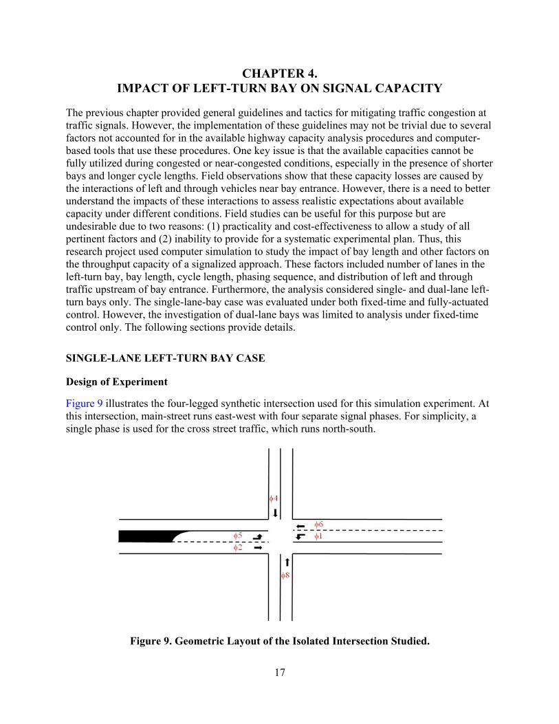
CHAPTER 4. IMPACT OF LEFT-TURN BAY ON SIGNAL CAPACITY
The previous chapter provided general guidelines and tactics for mitigating traffic congestion at traffic signals. However, the implementation of these guidelines may not be trivial due to several factors not accounted for in the available highway capacity analysis procedures and computer-based tools that use these procedures. One key issue is that the available capacities cannot be fully utilized during congested or near-congested conditions, especially in the presence of shorter bays and longer cycle lengths. Field observations show that these capacity losses are caused by the interactions of left and through vehicles near bay entrance. However, there is a need to better understand the impacts of these interactions to assess realistic expectations about available capacity under different conditions. Field studies can be useful for this purpose but are undesirable due to two reasons: (1) practicality and cost-effectiveness to allow a study of all pertinent factors and (2) inability to provide for a systematic experimental plan. Thus, this research project used computer simulation to study the impact of bay length and other factors on the throughput capacity of a signalized approach. These factors included number of lanes in the left-turn bay, bay length, cycle length, phasing sequence, and distribution of left and through traffic upstream of bay entrance. Furthermore, the analysis considered single- and dual-lane left-turn bays only. The single-lane-bay case was evaluated under both fixed-time and fully-actuated control. However, the investigation of dual-lane bays was limited to analysis under fixed-time control only. The following sections provide details.
SINGLE-LANE LEFT-TURN BAY CASE
Design of Experiment
Figure 9 illustrates the four-legged synthetic intersection used for this simulation experiment. At this intersection, main-street runs east-west with four separate signal phases. For simplicity, a single phase is used for the cross street traffic, which runs north-south.
Figure 9. Geometric Layout of the Isolated Intersection Studied.

18
Note that the eastbound approach has a single lane feeding traffic to the left-turn and through phases, whereas the westbound approach provides full lanes for the two movements. In the application of highway capacity analysis methods, users generally treat these cases as the same despite the knowledge that this is not always the case (17, 44). This deficiency is due to an absence of guidelines on how to account for the differences, which depend on multiple factors.
The objective of this simulation experiment is to better understand how various factors affect the capacity of left-turn and through signal phases receiving traffic from a single lane (eastbound approach in Figure 9). Thus, it is logical to compare the operational performance of this case against the ideal scenario represented by the westbound approach, using same demand and control conditions. As a result, the demands for movements on both approaches were kept the same. Furthermore, demands and signal timings were chosen to produce theoretical volume-to-capacity ratio close to one. For all cases, green splits were calculated using Webster’s equal saturation method implemented in PASSER V-09.
For comparison purposes, throughput (the number of vehicles crossing the stop bar) was
used as a proxy for the real capacity of the corresponding phases. Different conditions were produced by varying bay length, cycle length, phasing sequences, and left versus through traffic distribution. For reference purposes, westbound direction is termed as unrestricted approach. As such, the throughputs of westbound movements, taken as surrogate measures of ideal capacities, are termed as unrestricted capacities. The eastbound approach, on the other hand, is referred as the restricted approach. Consequently, the movements on this approach are termed as restricted movements.
VISSIM (45) was used for simulating seven volume settings, five cycle lengths, four
phasing sequences, and seven different bay lengths. These values produce 980 unique scenarios. For each scenario, researchers conducted five replications of simulation using different random seeds. This produced a total of 4,900 simulation runs, which were repeated for fixed-time and fully-actuated control cases. Each run consisted of a 15-minute warm-up period, followed by a one-hour data collection period. Table 2 provides values of factors simulated. Note that the total demand for each main street approach remained fixed at 1400 vehicles per hour (vph), but the distribution of left-turn versus through demand varied for the seven volume scenarios.
Table 2. Simulation Scenario Matrix.
Cycle Length
(sec)
Volume (vph) Phasing Sequence
Bay Length
(ft) Volume Index
Main Minor Left Through Through φ1 φ5
90 1 100 1300 200 Lead Lead 100 100 2 300 1100 200 Lead Lag 200 110 3 500 900 200 Lag Lead 300 120 4 700 700 200 Lag Lag 400 130 5 900 500 200 500
6 1100 300 200 600 7 1300 100 200 700
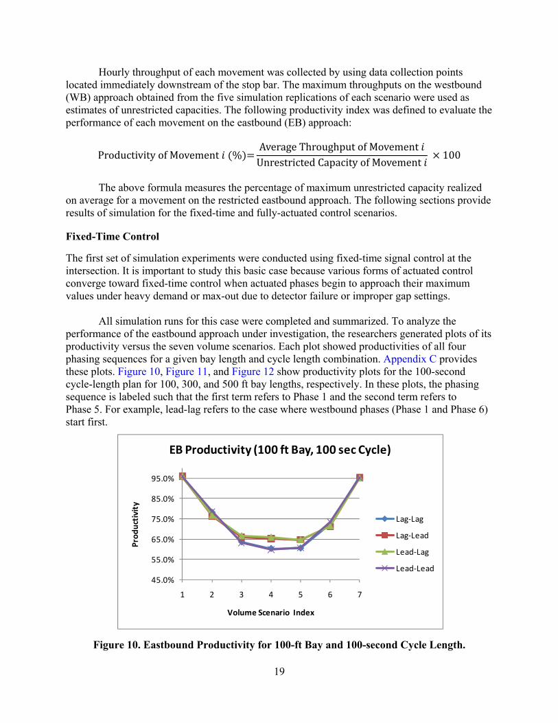
19
Hourly throughput of each movement was collected by using data collection points located immediately downstream of the stop bar. The maximum throughputs on the westbound (WB) approach obtained from the five simulation replications of each scenario were used as estimates of unrestricted capacities. The following productivity index was defined to evaluate the performance of each movement on the eastbound (EB) approach:
Productivity of Movement %Average Throughput of Movement
Unrestricted Capacity of Movement 100
The above formula measures the percentage of maximum unrestricted capacity realized on average for a movement on the restricted eastbound approach. The following sections provide results of simulation for the fixed-time and fully-actuated control scenarios.
Fixed-Time Control
The first set of simulation experiments were conducted using fixed-time signal control at the intersection. It is important to study this basic case because various forms of actuated control converge toward fixed-time control when actuated phases begin to approach their maximum values under heavy demand or max-out due to detector failure or improper gap settings. All simulation runs for this case were completed and summarized. To analyze the performance of the eastbound approach under investigation, the researchers generated plots of its productivity versus the seven volume scenarios. Each plot showed productivities of all four phasing sequences for a given bay length and cycle length combination. Appendix C provides these plots. Figure 10, Figure 11, and Figure 12 show productivity plots for the 100-second cycle-length plan for 100, 300, and 500 ft bay lengths, respectively. In these plots, the phasing sequence is labeled such that the first term refers to Phase 1 and the second term refers to Phase 5. For example, lead-lag refers to the case where westbound phases (Phase 1 and Phase 6) start first.
Figure 10. Eastbound Productivity for 100-ft Bay and 100-second Cycle Length.
45.0%
55.0%
65.0%
75.0%
85.0%
95.0%
1 2 3 4 5 6 7
Prod
uctivity
Volume Scenario Index
EB Productivity (100 ft Bay, 100 sec Cycle)
Lag‐Lag
Lag‐Lead
Lead‐Lag
Lead‐Lead

20
Figure 11. Eastbound Productivity for 300-ft Bay and 100-second Cycle Length.
Figure 12. Eastbound Productivity for 500-ft Bay and 100-second Cycle Length.
The following observations can be made by reviewing simulation results for this scenario provided in Appendix C:
• For a 100-ft left-turn bay, lead-lag and lag-lead phasing sequences produce higher productivity than the other two phasing sequences, especially at higher cycle lengths. For longer bays, however, the performance of these two phasing sequences becomes worst than lead-lead and lag-lag sequences.
75.0%
80.0%
85.0%
90.0%
95.0%
100.0%
1 2 3 4 5 6 7
Prod
uctivity
Volume Scenario Index
EB Productivity (300 ft Bay, 100 sec Cycle)
Lag‐Lag
Lag‐Lead
Lead‐Lag
Lead‐Lead
92.0%
93.0%
94.0%
95.0%
96.0%
97.0%
98.0%
99.0%
100.0%
1 2 3 4 5 6 7
Prod
uctivity
Volume Scenario Index
EB Productivity (500 ft Bay, 100 sec Cycle)
Lag‐Lag
Lag‐Lead
Lead‐Lag
Lead‐Lead

21
• Approach productivity is very high for cases where percent of left-turns is either very low or very high (i.e., volume scenarios 1 and 7). Productivity drops significantly as the distribution of left-turn and through traffic gets closer, with balanced scenario (volume scenario 4) being the worst.
• For all timing plans, there is no significant difference in the performance of the four
phasing sequences for bay lengths of 500 ft or higher. Maximum difference is within 3 percent. It is worth noting that the productivity of the best-case scenario is about 97 percent of the unrestricted cases. The reader should note that length of the left-turn bay controls the maximum number of
left-turn vehicles that can be stored in the bay. It also controls the maximum number of through vehicles that can store in the through lane downstream of entrance to the bay. In cases where either one or both of these storage spaces have filled, additional arriving vehicles (regardless of movement) form a single file (queue) upstream of bay entrance. Thus, separate left-turn and through signal phases work effectively only until their respective storage spaces have cleared (Stage 1). After that, the combined capacity of the two phases is determined by the shared arrivals of vehicles stored upstream of the bay entrance (Stage 2). For very short bays with high demand, the duration of Stage 1 is short (8–10 seconds) relative to Stage 2, producing capacities close to that of a shared lane at the stop bar. Under such conditions, it is beneficial to allow left-turn and through vehicles to move simultaneously. Even then, the approach capacity is only 65 percent of the unrestricted (westbound) approach. Messer and Fambro (44) reported similar observations. Their analytical simulation study found that lead-lag and lag-lead phasing sequences performed better for bay length shorter than 75 ft.
Theoretically, increasing the cycle length also increases phase capacity. In practice, however, this capacity increase can only be realized if no blocking occurs. Figure 13 explains this point by plotting productivity of the four phasing sequences for one sample case (300 ft bay, Volume scenario 3). Note that productivity reduces as cycle length increases.
Figure 13. Productivity of Restricted Approach versus Cycle Length.
75.0%77.0%79.0%81.0%83.0%85.0%87.0%89.0%91.0%93.0%95.0%
90 100 110 120 130
Prod
uctivity
Cycle Length (sec.)
EB Productivity (Volume Scenario 3, 300 ft Bay)
Lag‐Lag
Lag‐Lead
Lead‐Lag
Lead‐Lead

22
For the case represented in Figure 13, reductions in productivity are caused by blocking associated with long queues. For the same volume scenario, a longer bay will result in higher productivity by reducing blocking. On the other hand, larger cycle lengths will reduce productivity. These points can be observed from Figures 14, 15, and 16. Notice that a 400-ft bay is sufficient to attain 95 percent productivity for a 90-second cycle length, while larger bays are needed to achieve the same results for larger cycle lengths.
Figure 14. Approach Productivity for 90-second Cycle Length and Different Bay Lengths.
Figure 15. Approach Productivity for 110-second Cycle Length and Different Bay Lengths.
50.0%55.0%60.0%65.0%70.0%75.0%80.0%85.0%90.0%95.0%100.0%
100 200 300 400 500 600 700
Prod
uctivity
Bay Length (feet)
EB Productivity (Volume Scenario 3, 110 sec Cycle)
Lag‐Lag
Lag‐Lead
Lead‐Lag
Lead‐Lead
50.0%55.0%60.0%65.0%70.0%75.0%80.0%85.0%90.0%95.0%100.0%
100 200 300 400 500 600 700
Prod
uctivity
Bay Length (feet)
EB Productivity (Volume Scenario 3, 90 sec Cycle)
Lag‐Lag
Lag‐Lead
Lead‐Lag
Lead‐Lead
23
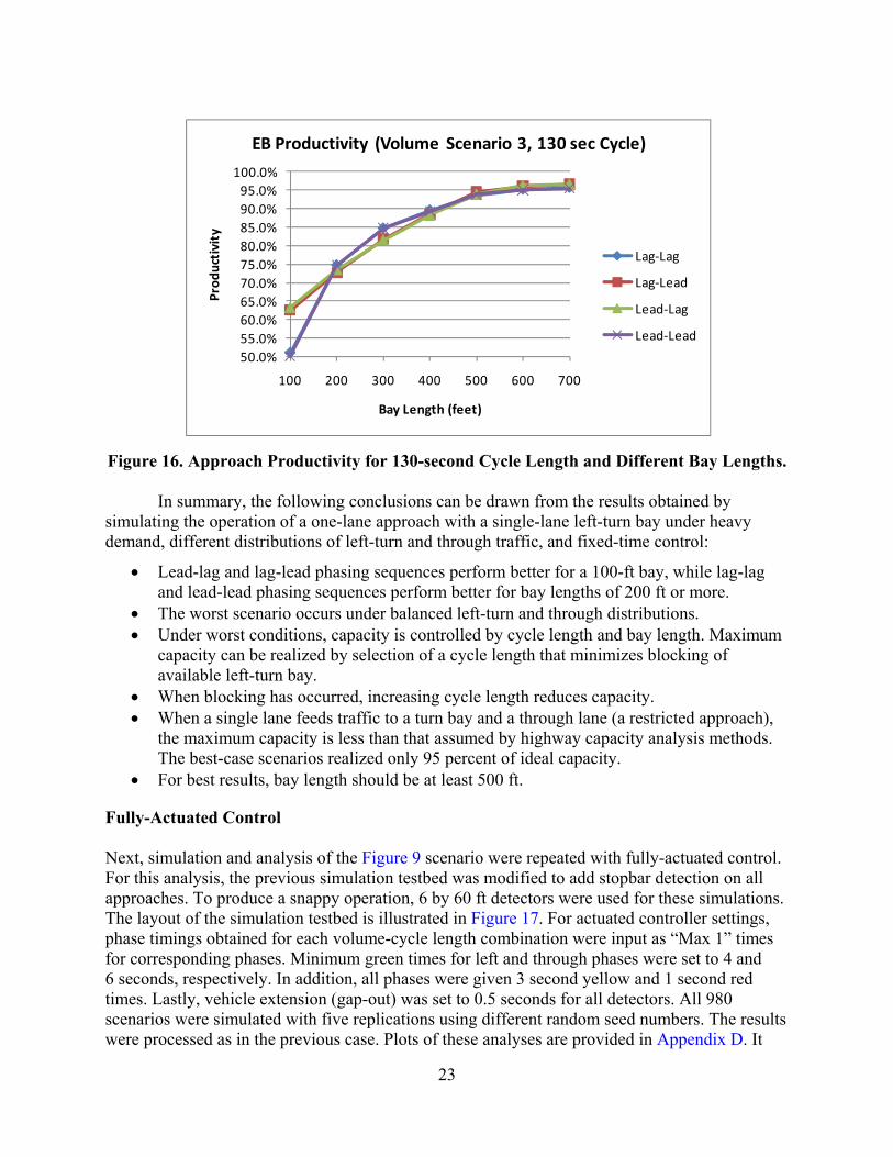
Figure 16. Approach Productivity for 130-second Cycle Length and Different Bay Lengths.
In summary, the following conclusions can be drawn from the results obtained by simulating the operation of a one-lane approach with a single-lane left-turn bay under heavy demand, different distributions of left-turn and through traffic, and fixed-time control:
• Lead-lag and lag-lead phasing sequences perform better for a 100-ft bay, while lag-lag and lead-lead phasing sequences perform better for bay lengths of 200 ft or more.
• The worst scenario occurs under balanced left-turn and through distributions. • Under worst conditions, capacity is controlled by cycle length and bay length. Maximum
capacity can be realized by selection of a cycle length that minimizes blocking of available left-turn bay.
• When blocking has occurred, increasing cycle length reduces capacity. • When a single lane feeds traffic to a turn bay and a through lane (a restricted approach),
the maximum capacity is less than that assumed by highway capacity analysis methods. The best-case scenarios realized only 95 percent of ideal capacity.
• For best results, bay length should be at least 500 ft.
Fully-Actuated Control Next, simulation and analysis of the Figure 9 scenario were repeated with fully-actuated control. For this analysis, the previous simulation testbed was modified to add stopbar detection on all approaches. To produce a snappy operation, 6 by 60 ft detectors were used for these simulations. The layout of the simulation testbed is illustrated in Figure 17. For actuated controller settings, phase timings obtained for each volume-cycle length combination were input as “Max 1” times for corresponding phases. Minimum green times for left and through phases were set to 4 and 6 seconds, respectively. In addition, all phases were given 3 second yellow and 1 second red times. Lastly, vehicle extension (gap-out) was set to 0.5 seconds for all detectors. All 980 scenarios were simulated with five replications using different random seed numbers. The results were processed as in the previous case. Plots of these analyses are provided in Appendix D. It
50.0%55.0%60.0%65.0%70.0%75.0%80.0%85.0%90.0%95.0%100.0%
100 200 300 400 500 600 700
Prod
uctivity
Bay Length (feet)
EB Productivity (Volume Scenario 3, 130 sec Cycle)
Lag‐Lag
Lag‐Lead
Lead‐Lag
Lead‐Lead

24
should be noted that the use of term “cycle length” here is only for reference/comparison purposes. Here, cycle length refers to the sum of max times of all phases in a ring. It should be noted that the actual time it takes to cycle through all phases varies under fully actuated control.
Figure 17. Layout of Stopbar Detector for Fully-Actuated Control. A review of simulation results showed that lagging phases with heavy demand provided higher throughput. Figure 18 illustrates this finding using the 300 ft bay plus 100 second cycle length case for all seven volume scenarios. While reviewing this figure, recall that volume scenarios 1, 2, and 3 have higher through demand, volume scenario 4 is balanced, and volume scenarios 5, 6, and 7 have higher left-turn demand.
Figure 18. Productivity of Restricted Approach Volume Scenarios under Fully-Actuated Control.
70.0%
75.0%
80.0%
85.0%
90.0%
95.0%
100.0%
1 2 3 4 5 6 7
Prod
uctivity
Volume Scenario Index
EB Productivity (300 ft Bay, 100 sec Cycle)
Lag‐Lag
Lag‐Lead
Lead‐Lag
Lead‐Lead

25
In this figure, note that:
• Lead-lead and lead-lag phasing sequences, in which the through phase of the restricted approach (Phase 2) is lagging, produce higher productivity for the first three volume scenarios.
• For volume scenarios 5, 6, and 7, lead-lag and lag-lag phasing sequences, in which left-turn phase on the restricted approach is lagging, produce higher productivity.
• As in the fixed-time control case, balanced scenario has the lowest productivity. • Lead-lag phasing performs consistently well but has slightly less productivity than the
other two sequences for more balanced volume scenarios. • The productivity of lag-lead phasing sequence, in which left-turn phase (Phase 5) on the
restricted approach leads is consistently worse than all other phasing sequences. Using the example of lead-lead phasing, Figure 19 explains why lagging heavier phases produces better results under actuated control. In this example, Phase 1 gaps out and terminates at time t1 and Phase 2 starts early. Under this scenario, Phase 2 reaches its maximum at t4 but does not terminate because it must cross the barrier at the same time as Phase 6. Since Phase 6 extends to its maximum value, Phase 2 gets additional time (capacity) it would not have received if Phase 1 was lagging. If Phase 2 has heavier demand than Phase 1, this scenario will help traffic served by it. On the other hand, lagging the lighter phase hurts the heavier phase. Improper phasing sequence under fully-actuated control may perform worse than the same sequence under fixed-time control. As an example, refer to Figure 11 that shows that the productivity for volume scenarios 6 and 7 (for the same bay length plus cycle length combination) was above 93 percent regardless of phasing sequence. However, that is not the case under actuated control as illustrated in Figure 18. Thus, it is more important to implement an appropriate phasing sequence under fully-actuated control.
Figure 19. Phasing Sequence Example for Fully-Actuated Control.
Simulation results (Appendix D) further show that, similar to using long cycle length in fixed-time control, increasing max times result in loss of capacity for the same reasons as described earlier. However, if phasing sequence is chosen properly, the impacts of longer max times are not as severe as longer cycle length under fixed-time control. This difference is due to the fact that the gapped phase gets serviced earlier next time under actuated control.

26
With regard to bay length, the researchers observed similar patterns as under fixed-time control. The productivity of the restricted approach was good for bay lengths of 500 ft or more. Under optimal phasing sequences, the productivity of restricted approach for all tested scenarios was in the neighborhood of 95 percent. The results of this investigation are summarized below.
• Lagging the phase with heavy demand produces higher throughput. • The maximum throughput of a restricted approach is 95 percent of the ideal case assumed
by Highway Capacity Manual (HCM) analysis procedures for a similar scenario. • Choice of phasing sequence has a bigger impact on capacity than that of fixed-time
control. • As in the case of fixed-time control, capacity (productivity) decreases with longer max
times. However, the impact is not as severe when appropriate phasing sequence is chosen.
• Bay length of 500 ft is sufficient when phasing sequence and cycle length are set properly.
Under actuated-coordinated control, the performance of signal operation will be bounded
by the fixed-time and fully actuated cases. For the gapped phase, the consequences will more likely be closer to the fixed-time control. However, as opposed to fixed-time case, another phase will get added capacity. Lack of time prevented a thorough study of this type of control.
SIMULATION EXPERIMENTS FOR DUAL LEFT-TURN BAY
Chapter 10 of HCM 2000 (46) recommends considering use of a dual left-turn bay when left-turn demand exceeds 300 vph. In the simulation experiment for the single left-turn bay case, left-turn demand for volume scenario 2 is 300 vph. Simulation results for this volume scenario revealed that with proper signal settings, approach productivity of around 90 percent can be achieved even for the 200-ft single-lane bay case. This observation warrants further investigation regarding the HCM recommended threshold.
To study the impact on throughput of dual left-turn bay, researchers repeated the previous fixed-time simulation study by adding a lane in the eastbound left-turn bay. All other variables remained the same. Two simulation experiments were carried out. The first experiment used the same phase times as in the previous case. The second experiment used revised signal timings obtained by explicitly considering two lanes in the bay.
Simulation Experiments Using Timings for the Single-Lane Case
Geometric layout for this case is shown in Figure 20. Notice that there is no additional lane in the westbound direction. This allows use of previous timings to study the benefits of adding a lane to the eastbound bay. As before, all 980 scenarios were simulated with five replications each. As before, plots of productivity were generated. Appendix E provides these plots.

27
Figure 20. Geometric Layout for Dual Left-Turn Bay Experiments.
These simulation experiments reveal that adding a lane in the bay without incorporating
its impact into derivation of phase times does have a positive impact on productivity, but that impact is not significant. Key observations from this set of simulations are listed below.
• Phasing sequence selection matters only in the 100 ft bay case. In this case, performance
of lead-lead and lag-lag phasing sequences worsens significantly for cycle lengths larger than 120 seconds. In all other cases, the performance of different phasing sequences is about the same.
• As expected, there is a rightward shift in productivity. In other words, adding a lane helps cases with heavier left-turn demand. However, the best-case scenario is not better than the single-lane case.
• For the 300 vph left-turn demand case (HCM threshold mentioned above), adding another lane to the bay only helped when the bay length was 100 or 200 ft. For longer bay lengths, there was no improvement in productivity.
Simulation Experiment with Revised Timings
Next, the impact on productivity of a dual-lane left-turn bay with revised signal timings was studied. To make proper conclusions, a full left-turn lane was also added in the westbound direction. Figure 21 shows the layout of the simulated intersection for this case. This simulation experiment used the same data as before (see Table 2), but signal timings were recalculated to account for added left-turn lanes in both directions. Because of an added lane, but unchanged demand loading, throughput of westbound movements could no longer be used as a proxy for ideal capacities. Therefore, researchers used the following alternate method for calculating productivity of each eastbound movement:
Eastbound Demand Served % Measured Eastbound Throughput
Eastbound Demand 100
φ2
φ8
φ4
φ5φ1φ6

28
Figure 21. Geometric Layout with Dual Left-Turn Lanes.
The above estimate of approach productivity is similar to the one used for previous
experiments. To verify this observation, the researchers compared the two measures of productivity for three selected single left-turn lane fixed time cases used as an example previously. Appendix F provides plots for these three cases corresponding to 100-second cycle length and bay lengths of 100, 300, and 500 ft. By reviewing these plots against those provided before, it is clear that the two measures are similar. Minor differences observed are due to the fact that the denominator in the above equation is a deterministic value, while the denominator used in the original equation (Page 19) was calculated using VISSIM output that had random variability.
Appendix G provides productivity (percent of demand served) plots for all these cases. From the simulation results, researchers observed the following:
• For the 100-ft bay case, the results were about the same as having a single lane in the bay. Similarly, lead-lag and lag-lead phasing sequences were better and for the same reasons.
• For the 200-ft bay case, productivity was higher by a few percent as compared to the single-lane case.
• For bay lengths of 200 ft or more, lead-lead and lag-lag phasing sequences were better. • Productivity become stable at around 99 percent as bay length approached 500 ft. A
400-ft bay also produced similar results when the cycle length was 100-second or lower and lead-lead or lag-lag phasing sequences were selected.
Thus, adding a second lane in the left-turn bay improved the productivity for bay lengths
of 200 ft of more. In addition, the best-case productivity was almost the same as ideal productivity, which was not the case with a single-lane case. However, before adding a lane, any impacts on phase times due to pedestrian requirements should be investigated.
φ2
φ8
φ4
φ5φ1φ6
29
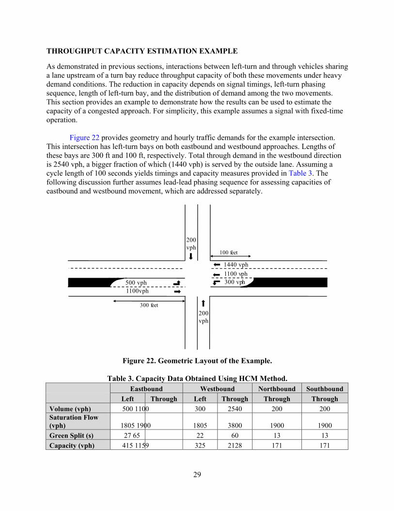
THROUGHPUT CAPACITY ESTIMATION EXAMPLE
As demonstrated in previous sections, interactions between left-turn and through vehicles sharing a lane upstream of a turn bay reduce throughput capacity of both these movements under heavy demand conditions. The reduction in capacity depends on signal timings, left-turn phasing sequence, length of left-turn bay, and the distribution of demand among the two movements. This section provides an example to demonstrate how the results can be used to estimate the capacity of a congested approach. For simplicity, this example assumes a signal with fixed-time operation. Figure 22 provides geometry and hourly traffic demands for the example intersection. This intersection has left-turn bays on both eastbound and westbound approaches. Lengths of these bays are 300 ft and 100 ft, respectively. Total through demand in the westbound direction is 2540 vph, a bigger fraction of which (1440 vph) is served by the outside lane. Assuming a cycle length of 100 seconds yields timings and capacity measures provided in Table 3. The following discussion further assumes lead-lead phasing sequence for assessing capacities of eastbound and westbound movement, which are addressed separately.
Figure 22. Geometric Layout of the Example.
Table 3. Capacity Data Obtained Using HCM Method. Eastbound Westbound Northbound Southbound Left Through Left Through Through Through Volume (vph) 500 1100 300 2540 200 200 Saturation Flow (vph) 1805 1900 1805 3800 1900 1900 Green Split (s) 27 65 22 60 13 13 Capacity (vph) 415 1159 325 2128 171 171
200vph
1100 vph1440 vph
300 vph500 vph1100vph
200vph
300 feet
100 feet

30
Eastbound approach has a 300-ft bay, so we can use Figure 11 to assess its throughput capacity. For this approach, note that left-turn traffic (500 vph) is 31 percent of the total eastbound traffic. Furthermore, note that this percentage is between volume scenarios 2 (21 percent left-turn demand) and 3 (35 percent left-turn demand). Using interpolation, the estimated throughput capacity of eastbound traffic is estimated to be 90 percent of ideal capacity provided in the above table. Therefore, the estimated capacity for the left-turn movement is equal to 374 (415 × 0.9) vph and for the through movement is 1043 (1159 × 0.9) vph. For the westbound approach, throughput capacity estimation procedure requires an additional step because of multiple lanes serving the through traffic. The first step prorates total capacity according to lane distribution of through traffic, which are: 43.3 percent (1100 vph ÷ 2540 vph) and 56.7 percent (1440 vph ÷ 2540 vph), for inside and outside lanes, respectively. Using these percentages, through capacities of these lanes are 921 (2128 × 0.433) vph and 1207 (2128 × 0.567) vph, respectively. The next step is to account for interactions between left and through vehicles in the inside lane. The demand scenario for the inside lane is the same as volume scenario 2. Thus, capacity adjustment factor can be obtained from Figure 10, which provides results for the 100-ft bay case. From this figure, the productivity for volume scenario 2 is approximately 80 percent of ideal capacity. Thus, the capacities of the left-turn and through movements are estimated to be 260 (325 × 0.8) vph and 737 (921 × 0.8) vph, respectively. Finally, the total capacity of the through phase is the sum of through capacities of the two lanes, which is equal to 944 (737 + 1207) vph.
CONCLUSIONS
At a congested intersection approach with a left-turn bay, interactions of through and turning vehicles near the bay entrance often cause loss of valuable capacity. In this research project, the researchers conducted controlled simulation experiments to study the impacts of such interactions on signal capacity. Specifically, these simulation experiments studied the impacts of cycle length, phasing sequences, distribution of left and through vehicles, and length of turn bay on the capacity of left and through vehicles sharing a lane upstream of the bay. For the single-lane case, the impacts of fixed-time and fully actuated control were studied. Due to time limitations, researchers studied the dual-left bay case only for fixed-time control. Analysis of results from these experiments provided useful insights. Key observations from this analysis are:
• The worst scenario occurs when there is equal distribution of left and through vehicles in the lane feeding traffic to the left-turn bay.
• When blocking occurs, increasing cycle length decreases capacity. • When appropriate cycle length and phasing sequence are selected:
o a 500-ft single-lane is sufficient to provide the maximum capacity, which is 95 percent of the ideal capacity, and
o a 400-ft dual-lane bay is sufficient to provide up to 99 percent of ideal capacity. • For fixed-time control:
o lead-lag and lag-lead phasing sequences perform better for 100-ft bays; and o for bay lengths of 200 ft or more, lag-lag and lead-lead phasing sequences
perform better, with their benefits diminishing for bay lengths of 500 ft or longer.

31
• For actuated control (tested for single-lane bays only): o lagging the phase with heavy demand movements improves throughput; o choice of phasing sequence has bigger impact on capacity than that for fixed-time
control; and o larger cycle lengths decrease capacity, but the adverse impact is less with properly
selected phasing sequence setting.


33
CHAPTER 5. APPLICATIONS TO REAL PROBLEMS
As the final task of this project, limited field studies were conducted. The purpose of these studies was twofold: (1) to apply the guidelines developed to real world problems and (2) to refine the guideline based on the actual application. For these field studies, researchers collected data for a small three-intersection system in College Station, Texas, and three intersections in Austin, Texas. Data collection at the first site consisted of in-field manual data collection, extraction of data from videos recorded from the roof of a nearby parking garage next to the site, and videos recorded from a surveillance camera at one of the intersections. For the Austin sites, data came from videos recorded by the City of Austin at sites selected by the researchers after field visits. After reviewing the data, the three-intersection system in College Station and one intersection in Austin were chosen for further study.
THREE-INTERSECTION SYSTEM IN COLLEGE STATION
This system is located to the south of Texas A&M University (TAMU) campus in College Station. It consists of two signalized intersections (Olsen Boulevard at George Bush Drive and Wellborn Road at George Bush Drive) with an unsignalized one-way stop controlled T-intersection (Marion Pugh Drive at George Bush Drive) in the middle. In addition, there is an at-grade railway crossing, with 27–30 trains per day, next to the intersection of Wellborn Road and George Bush Drive. Wellborn Road and Olsen Boulevard are approximately 850 ft apart, while the segment between Marion Pugh Drive and Wellborn Road is about 400 ft in length. Figure 23 shows the layout of this system.
Figure 23. Three-Intersection System at George Bush Drive in College Station, Texas.

34
The two signals at this site operate with fully-actuated control. Previous attempts to provide coordination have failed due to sharp fluctuations between peak-period demands and origin-destination (O-D) patterns resulting from various class schedules. Existing control included partial metering at Olsen Boulevard during the p.m. peak period. The city implemented this strategy by using special functions to put max recalls on westbound left-turn and northbound phases. For vehicle detection, the Olsen Boulevard intersection uses inductive loops, while the Wellborn Road intersection uses video cameras. Furthermore, the Wellborn Road intersection is on several shuttle bus routes operated by TAMU Transportation Services. By law, all buses must stop before crossing the railroad tracks. This policy affected one bus route for which buses travel westbound through the Wellborn Road intersection and turned left on Marion Pugh. Returning buses on this route turn right from Marion Pugh and travel eastbound through Wellborn Road. In addition to the normal peaks, demand at the study site increases abruptly for a brief period between classes, which have different schedules for odd and even days of a normal week. Affected locations during evening demand surges include: southbound approach at Olsen Boulevard, southbound approach at Wellborn Road, and eastbound approach at Wellborn Road and George Bush Drive.
Application of General Congestion Management Guidelines
Step 1: Identify the Highest Priority Location Needing Congestion Mitigation
Researchers selected the p.m. peak period for this task and conducted several scouting trips to the field site during the week of January 19, 2009. The purpose of these trips was to observe traffic conditions to: better understand traffic patterns and problems, determine duration of the p.m. peak period, and identify how detailed data could be collected. During these trips, researchers collected sample data on vehicle departure headways for several approaches, conducted a pilot study to verify the notion of tracking cyclic queue growth to accurately estimate demand, observed effect of buses on signal operation, and identified resources available/needed for detailed data collection.
These observations verified that Wellborn Road at George Bush Drive is the critical intersection in this system. Depending on the day of the week, queuing problems at this intersection began as early as 3:00 p.m. and became worse shortly after 5:00 p.m. In general, congested conditions lasted until around 6:00 p.m. During this period, researchers observed long queues in all four directions at the Wellborn Road intersection. Of these, the westbound queue frequently blocked the left-turn bay and eastbound queue backed up and blocked the upstream intersection at Olsen Boulevard. When the latter condition occurred, it worsened queuing on the southbound approach at Olsen Boulevard. Approximately 30 buses per hour crossed the railway tracks from both eastbound and westbound directions. Each bus stopped before crossing the railway tracks, wasting between 4 to 6 seconds of green capacity of the lane it was in.
Researchers also found that observing cyclic queues for better demand estimation becomes almost impossible in several cases when:
• there is a sudden surge in demand producing rapid queue growth; • view of queue is obstructed by vehicles in the adjacent lane;

35
• a queue grows beyond the point from where downstream signal operation cannot be seen clearly or movement of the back of queue cannot be linked to a signal operation reference point (i.e., end or green); and/or
• entrance to a bay is blocked.
Also, it was not easy to count vehicles in long queues at any given point in time. The researchers were able to accurately estimate lengths of visible queues by comparing them to pre-measured reference points (landmarks) on the roadway and only when queue length were stable.
Step 2: Examine and Fix Any Problems with Field Equipment
During field trips, researchers observed that the westbound through phase at the Wellborn Road at George Bush Drive intersection did not gap out as expected in most signal cycles. Further investigation revealed that the detector was often placing false calls causing the phase to keep extending even when there was no vehicle at the approach. The exact cause of this problem could not be ascertained. This type of problem is common with video-based detection.
Step 3: Conducted Data Collection
The researchers collected detailed data using a combination of in-field manual counts and in-lab processing of videos recorded in the field. After getting permission from the property owner, the researchers placed two video cameras on the roof of a parking garage to record the traffic operations at Olsen Boulevard and Marion Pugh Drive. Figure 24 and Figure 25 illustrate views from these two cameras. For the Wellborn Road intersection, the researchers utilized two surveillance cameras located in the southeast and southwest quadrants at this intersection. A communications link exists between these cameras and the TransLink® laboratory at TTI. Video feeds from these cameras were simultaneously recorded using a digital recorder. To facilitate offline processing, a scan converter was used to feed video screen from a computer showing a clock. Figure 26 illustrates a screen showing all three data feeds. As shown, data for northbound, southbound, and westbound approaches were collected from screen 1, while data for the eastbound approach was collected from screen 3.
In-field data was collected from 3:30 p.m. to 5:30 p.m. on Wednesday, January 28, 2009. Data collection was terminated before end of peak period because it became completely dark around 5:30 p.m., making it difficult to extract data from the videos after that point. During this time, several researchers simultaneously observed operations from different locations. One researcher manually recorded vehicle counts at Marion Pugh. Later, researchers extracted turning-count data for the two intersections from the recorded videos. To facilitate this process, they used a computer program to manually record the passing of each vehicle across a preselected reference point. These data were then processed to obtain 15-minute counts. The data collection process also provides headway data, but these data were not used in the project. Additionally, researchers obtained controller settings from city’s controller database via access provided to them by the city staff. It should be noted that the Wellborn Road intersection uses split phasing on eastbound and westbound approaches, and the Olsen Boulevard intersection uses split phasing on the northbound and southbound approaches.

36
Figure 24. Video Capture of Olsen Boulevard at George Bush Drive.
Figure 25. Video Capture of Marion Pugh Drive at George Bush Drive.

37
Figure 26. Video Capture of Wellborn Road at George Bush Drive.
Step 4: Analyze Data, Formulate, and Implement Strategies
Since there is lack of analytical tools suitable for application to congested systems, researchers decided to use VISSIM-based computer simulation to analyze various options. Even though there are limitations associated with simulation models, they are better than analytical models. Their advantages include the ability to provide full experimental control, emulation of stochastic variability, and detailed data collection abilities. Their disadvantages include a time consuming modeling and calibrating process and their inability to explicitly model several roadway features including two-way left-turn lanes and tapers. In addition, it is impossible to calibrate simulated sensors to match the operation of video-based sensors. Demand inputs to the simulation model were updated every 15 minutes according to the 15-minute counts collected from field data. Simulation models also require accurate input of O-D data. Since such information was not collected in the field, researchers derived that information synthetically using volume counts. For example, volume of southbound left-turns from Olsen Boulevard making a right-turn at Wellborn, Now (SB), was estimated as follows:
1. Let Nom (EB) be the estimate of southbound left-turns from Olsen Boulevard going through at Marion Pugh Drive toward Wellborn Road. Then:

38
Nom (EB) = Southbound Left-Turn Volume at Olsen × Percentage of Through Traffic on Eastbound Marion Pugh
2. Use eastbound through count at Olsen Boulevard, Nom (EB), to estimate Now( SB) as:
Now (SB) = Nom (EB) × Percentage of Right-Turn Traffic on Eastbound Wellborn
The VISSIM model was developed and calibrated after obtaining all necessary information. For Olsen Boulevard, sensors were placed to exactly match the existing loops. For the Wellborn Road at Bush intersection, field measurements of video-based detection zones were used to estimate lengths of sensors. Figure 27 shows a screenshot of the simulated facility. For reference purposes, this simulation model is referred to as the base model. Information on queue at each approach was collected from the model. Also collected were the start and end times of each phase during the simulated period.
Figure 27. Screenshot of VISSIM Model of the College Station Site.
Next, new timing strategies were developed and implemented in the simulations. These strategies were aimed at queue management by shortening maximum phase times at the Wellborn Road intersection and gating/metering at Olsen Boulevard. The rationale of using these strategies was as follows.
• As mentioned earlier, several traffic movements at this site experienced frequent cycle failures resulting in blocking. These cycle failures were due to demand surges associated with the class schedule (including shuttle bus schedule) and p.m. peak demand generated by university staff leaving after work. Queues forming prior to 5:00 p.m. are temporary and dissipate within a few cycles as the sudden surge in demand drops quickly. During this time, it is more important to manage queues than throughputs. Queue management is especially critical for the eastbound traffic on George Bush Drive between Olsen

39
Boulevard and Wellborn Road, as blockage of the link between the two signals further degrades the system operations.
• To minimize the risk of blockage on Olsen Boulevard due to queue overflow from
George Bush Drive, the City of College Station has been using a gating strategy at the Olsen Boulevard intersection. This gating strategy (see Figure 28) is implemented by using a special function in the controller to place max recalls on westbound left-turn phase (Phase 1) and northbound phase (Phase 3). These phases cater to a student dormitory and normally serve only a few cars per cycle in most cases. Forcing these phases to max out effectively meters demand from the other two phases feeding traffic to the eastbound approach at Wellborn Road intersections. This strategy also provides reasonably good operation for to-from movements at the unsignalized intersection in the middle.
Figure 28. Phase Numbering at Olsen Boulevard and George Bush Drive Intersection.
• A review of existing signal timings revealed the city was using maximum green times of relatively long duration, with the sum of critical max times equal to 186 and 154 seconds for the Wellborn Road and Olsen Boulevard intersections, respectively. These long max times and a sluggish operation (due to large gap settings) was a major factor in producing

40
long queues. Shortening max times would produce shorter queues, as long as enough capacity is provided.
At this site, both traffic signals operate in fully-actuated mode. For fully-actuated
controller, actual phase lengths are governed by a combination of real-time demand, detection zone, and gap settings. With improper settings, a phase may gap out prematurely or continue well beyond the presence of demand. Both situations can cause inefficient operation. Thus, selecting a proper setting for each phase is important to ensure proper operation during all conditions. Max time for each phase should be selected to provide sufficient capacity. For congested conditions, where the controller operation mimics fixed-time control, max times can be derived using the same procedure as that used for fixed time control. This procedure starts by determining the minimum delay cycle length followed by allocating effective green to all phases to provide equal degree of saturation. Critical 15-minute demand rate can be used for this purpose.
Researchers used performance analysis feature of PASSER V-09 to get an idea about appropriate ranges of cycle lengths for the two intersections. Figure 29 shows PASSER V performance analysis for the Wellborn Road at George Bush intersection. In this figure, the horizontal line represents demand. Notice that the cycle length must be longer than 105 seconds to provide sufficient capacity to handle demand. In addition, notice that the minimum delay cycle length is 110 seconds. Thus, the proper range of cycle lengths to investigate should be within the range of 110 to 186 (the sum of existing maximum times) seconds.
Figure 29. Performance Analysis for Wellborn Road and George Bush Drive Intersection.

41
The process was repeated for the intersection of Olsen Boulevard and George Bush Drive. At this intersection, the westbound right-turn traffic is serviced by and overlap of Phases 4 and 6 (see Figure 28). Since PASSER V does not explicitly handle this situation, westbound right-turn volume was adjusted as if it were only served by Phase 6. Figure 30 shows the PASSER V performance chart of this intersection. Notice that the minimum cycle length that provides sufficient capacity is for this intersection is 110 seconds and the minimum delay cycle length is 115 seconds. Hence, the proper cycle length ranges from 115 to existing 164 seconds.
Figure 30. Performance Analysis for Olsen Boulevard and George Bush Drive Intersection. Though there is no fixed cycle length during actuated control, a proxy cycle length can be defined as the time between the onsets of consecutive greens for a selected phase. It is conjectured that the proxy cycle length will be close to the sum of effective green times during congested conditions. Thus, simulation can be used to obtain required base cycle length using an iterative process as follows:
1. Select the longest desired cycle lengths for each controller and derive maximum phase times using this cycle length.
2. Program these times into the model and run the simulation. 3. From simulation results, calculate average proxy cycle length during the data collection
period. 4. If average proxy cycle length is close to the base cycle lengths used for the current
simulation model, the current max times are appropriate and could be used for implementation.
5. Otherwise, use the proxy cycle length to derive the phase max times and go to step 2.

42
The researchers repeated several iterations of the above steps by simulating proxy cycle lengths for both intersections. In the process, PASSER V was used to derive timings for Wellborn Road intersection corresponding to all proxy cycle lengths. However, a different procedure had to be used to derive phase timings for Olsen Boulevard intersection. The reason is that PASSER V’s phase time calculations cannot accurately accommodate the special (metering and overlap) situations to be implemented at this intersection. To obtain appropriate timing for the Olsen Boulevard intersection, a custom spreadsheet-based methodology was developed. This methodology explicitly accommodates the overlap phase in that it adjusts volume-to-saturation flow (v/s) ratio of the westbound right-turn movement by subtracting from it the v/s ratio of Phase 4 (overlap phase). Using the adjusted v/s ratios, green time of each phase was calculated. Phase times were also adjusted to accommodate minimum green times. In the cycle length search process, proxy cycle lengths used in simulation iterations 2 and higher were rounded to the nearest number divisible by 10. This was done for convenience in deriving phase times. To emulate the operation of a bad video detector for the westbound approach at the Wellborn Road intersection, researchers set max recall on this phase. Furthermore, the processes of buses stopping before crossing railway tracks in eastbound and westbound directions and causing loss in capacity were modeled by implementing bus stops with 2- and 3-second dwell times, respectively. Different dwell times were used to account for difference in approach grades. Table 4 shows the results these iterations.
Table 4. Results of the Cycle Length Search Process.
Olsen Boulevard
and George Bush Drive Wellborn Road
and George Bush Drive
Iteration Sum of Max
Times Average Proxy Cycle Length
Sum of Max Times
Average Proxy Cycle Length
1 164 130 186 169 2 130 105 170 145 3 120 103 140 125 4 120 103 130 117
In Table 4, notice that the average proxy cycle length for the Olsen Boulevard intersection was 105 seconds at iteration 2. Since the search range of cycle length at this intersection starts from 115 seconds and cycle length are rounded as specified above, a 120-second cycle length was used instead for the next iteration. Corresponding to the final timing with 130 and 120 seconds proxy cycle lengths for Wellborn Road and Olsen Boulevard intersections, respectively, maximum queue lengths and average queue lengths at each approach were collected from the simulation. Table 5 summarizes these results.

43
Table 5. Maximum and Average Queue Lengths in Feet.
In Table 5, notice that the queuing condition improved significantly for the eastbound approach at Wellborn Road intersection when new timings were used. The maximum queue length and average queue length for this approach were shortened from 850 ft to 442 ft and 301 ft to 110 ft, respectively. In other words, these reductions were 48 percent and 64.5 percent, respectively. For other approaches, the maximum and average queue lengths were not very sensitive to the changes in phase times. Observations of simulation indicated the need to make minor adjustments to max times, while keeping the same cycle length at this intersection. Using judgment, researchers reduced max times for northbound and southbound through phases by 4 seconds and increased times for eastbound and westbound (split) phases by 2 seconds. Furthermore, researchers increased the cycle length for Olsen Boulevard intersection from 120 seconds to 130 seconds. This change would require an appropriate offset in case it was decided to provide coordination between the two intersections. Table 6 provides maximum and average queues lengths from simulation after implementing these revisions.
Table 6. Maximum and Average Queue Lengths of the Proposed Timing Plan.
These new timings do not have any significant impact on Wellborn Road intersection but improved the eastbound traffic at Olsen Boulevard intersection. Thus, the researchers proposed these timings to the city staff for implementation. The proposed timing plan is shown in Table 7 and was first implemented in October 2009.
Table 7. Proposed Max Time Settings for College Station Site.
To study the impact of fixed westbound detector at the Wellborn Road intersection, researchers repeated the above mentioned iterations of simulations by removing the max recall from this phase. Table 8 provides the results of this analysis. Notice that the final cycle lengths
Left Through Left Through Left Through Left ThroughMax Queue (ft.) 232 206 91 429 96 372 850 518 393 391 497 499Avg Queue (ft.) 11 34 4 21 10 89 301 110.5 82 86 112 112Max Queue (ft.) 253 189 94 316 107 284 442 674 345 343 455 453Avg Queue (ft.) 13 30 5 21 7 60 110 108 58 62 78 74
North Bound South BoundOlsen Boulevard and George Bush Drive Wellborn Road and George Bush Drive
Original Timing
East Bound
West Bound
New Timing
East Bound West Bound North Bound
South Bound
Olsen Boulevard at George Bush Drive WBL EBT SBT EBL WBT NBT
Phase 1 2 3 4 5 6 7 8 Max Green 20 25 38 22 23 23 Wellborn Road at George Bush Drive
NBL SBT WBT SBL NBT EBT Phase 1 2 3 4 5 6 7 8 Max Green 18 36 23 28 26 29
Left Through Left Through Left Through Left ThroughMax Queue (ft.) 171 163 94 318 118 291 473 676 344 342 437 436Avg Queue (ft.) 9 25 3 21 8 58 101 107 59 64 84 80
Olsen Boulevard and George Bush Drive Wellborn Road and George Bush DriveEast Bound West Bound North
BoundSouth Bound
East Bound
West Bound
North Bound South Bound

44
are the same as the previous runs. This is an indication that the reductions in max times to obtain new values removed any adverse impacts of maxing out due to bad detection.
Table 8. Results of the Cycle Length Search Process if Equipment Is Fixed.
Olsen Boulevard
and George Bush Drive Wellborn Road
and George Bush Drive
Iteration Sum of Max
Time Average Proxy Cycle Length
Sum of Max Time
Average Proxy Cycle Length
1 164 129 186 150 2 130 105 150 129 3 120 104 130 116
Step 5: Repeat for Continual Improvement
Based on previous observations, the new timing plan was proposed for the 3 p.m. to 6 p.m. time window. After implementation of this timing plan in October 2009, field observations were conducted over a course of several days. Researchers quickly noticed the absence of expected improvements predicted by the simulation model. It did not take long to notice that traffic patterns had changed significantly from the original ones for which new timings were developed. One main reason of this change was the closure of a nearby roadway (Route Boulevard) on the TAMU campus. Implemented to facilitate a major building reconstruction project, this closure resulted in additional east-west traffic demand, including an additional westbound bus route through the system. Researchers also observed significantly more traffic on eastbound and southbound approaches at the Olsen Boulevard intersection. The increase in eastbound direction could be due to two new apartment complexes on FM 2818 located about two miles to the west of this system. For these drivers, George Bush Drive provides the shortest route to the center of the town. Despite significant increase in traffic demands and changes in traffic patterns, significant improvement could be seen for both northbound and southbound traffic at the intersection of George Bush Drive and Wellborn Road. The westbound and eastbound approaches at this intersection still faced cycle failures, continuing to cause blocking of the left-turn bay and the upstream signal at Olsen Boulevard. These queues did exhibit diminishing trends as time progressed; however, queues significantly increased when the old off-peak timing plan with larger max times kicked in at 6 p.m. This observation indicated that the new timings were working for these two approaches as well, but increased traffic demand had masked the improvements.
Computer simulation had predicted that running both signals at a 130-second cycle provided beneficial natural coordination when all phases at both signals started to max out. However, this benefit was not achieved in the field on a consistent basis because traffic conditions dictated the quality of natural synchronization on a day-to-day basis. Often, traffic conditions led to the worst possible natural coordination with undesirable results, where either Phase 2 or Phase 4 on Olsen Boulevard consistently suffered until one of these phases started to gap out. To eliminate this problem, researchers changed the operation of this intersection by slightly reducing the max times of Phases 2 and 4. These changes produced the desired effect of distributing adverse impacts between the two movements over the course of a few cycles instead of one phase suffering for the entire congested period. Researchers also increased eastbound
45
through max time at the Wellborn Road intersections by 4 seconds, changing the maximum cycle length to 134 seconds. This change produced minor improvement to the eastbound through phase, but it was not sufficient to completely eliminate the queuing problem. The only other timing alternative to improve eastbound through movement at this intersection was to eliminate split phasing in the east-west directions at this intersection. After observing space used by the two left-turn movements, researchers recommended this option to the city. After careful consideration, the city changed the operation to lead-lead left-turn phases with overlap. Observations by researchers have shown this change to produce significant improvement for the westbound movement at this intersection. Since this improvement was implemented several months after the official termination of this project, researchers did not conduct a detailed evaluation of signal operation afterwards.
SIGNALIZED INTERSECTION IN AUSTIN
In communications with researchers during the early phase of this project, City of Austin staff had indicated that any one of their numerous congested intersections could be used as test cases for this project. Researchers decided to accept this offer. Accompanied by members of the TxDOT advisory panel and City staff, they visited several sites of concern in Austin on June 2, 2009. These sites included a multi-jurisdiction signal system and two intersections. City staff also named another intersection of concern, but researchers did not have time to visit this additional location. Because these site visits occurred during off-peak times, researchers did not observe congestion or other operational problems at any of these sites. After discussing options, it was agreed that the city staff would video-record operations of the three signals of concern during evening peak periods and send these videos to the researchers for further evaluation. Because each intersection had a single surveillance camera, approaches could be recorded one at a time only in a selected sequence. Researchers received these videos and additional information several weeks later.
Application of General Congestion Management Guidelines
Step 1: Identify the Highest Priority Location Needing Congestion Mitigation
All three videotaped signals from Austin are parts of separate coordinated systems. For this reason, any congestion-reduction options were limited. Researchers conducted preliminary evaluation of videos and selected the intersection of Courtyard Drive and US 360 for further analysis. According to preliminary analysis, it was possible to achieve the most improvement at this location, while staying within the constraint of existing coordination with adjacent signals along US 360. Adjacent signals on both sides are approximately one mile away.
The Courtyard Drive intersection experiences heavy demand on the two high-speed US 360 approaches during evening peak period. Because of long cycle length and heavy through demand during the evening peak period, long queues form on both these approaches. However, through phases have sufficient capacity to clear these queues. Traffic on the eastbound approach (Courtyard Drive) is normally light but peaks immediately after 5:00 p.m. due to several office buildings located on the west side of Courtyard Drive. Peak period demand surge is of short duration but results in cycle failures for almost 45 minutes after the hour. Figure 31 shows a satellite view of this intersection obtained from Google maps.

46
Figure 31. Signalized Intersection at US 360 in Austin, Texas.
Step 2: Examine/Fix Field Equipments
On-site observations and preliminary evaluation of video recording showed no equipment failures at this site.
Step 3: Conduct Data Collection
This site has a surveillance camera installed at the northeast corner of the intersection (Figure 32). City of Austin staff videotaped the operation of this facility during evening peak hours. Since there is only one camera available at this location, video for each view had to be recorded one at a time. Video of view A was recorded on June 24, 2009, from 4:38 p.m. to 5:23 p.m. and that of view B was recorded on the same day from 5:24 p.m. to 6:09 p.m. Video for view C was recorded on June 25, 2009, from 5:00 p.m. to 6:00 p.m. Samples of video views A, B, and C are illustrated in Figure 33, Figure 34, and Figure 35, respectively. After initial analysis, the researchers decided to not use data from view C because it provides partial information and only for one major through movement. Data from the other two views were manually collected using an existing computer program. City of Austin staff also provided

47
timing plan information for this site. During the p.m. peak period, the city operates this intersection as part of a coordinated system with a cycle length of 150 seconds. Phase 3 serves eastbound approach and receives 19, 4, and 3 second max green, yellow, and all-red intervals, respectively. Northbound and southbound through movements receive 83 and 76 seconds of minimum greens, respectively, with 6 second yellow intervals and 2 second all-red intervals.
Figure 32. Camera Location and View Direction at US 360, Austin, Texas.
Figure 33. Screenshot of View A.

48
Figure 34. Screenshot of View B.
Figure 35. Screenshot of View C.

49
Step 4: Analyze Data, Formulate, and Implement Strategies
During the study period, eastbound was the only approach at this intersection with operations problems. This approach (Figure 32) has two lanes. The inside lane is exclusive for left-turn traffic. The outside lane allows shared movement of left-turn, through, and right-turn traffic. The flare at the intersection has enough room to store one right-turn vehicle next to vehicles queued in the outside lane. During the 40-minute period, researchers counted 178 left turns from the inside lane and 224 vehicles served by the outside lane. These 224 vehicles included 87 left turns, 137 right turns, and zero through vehicles. Figure 34 provides conditions at this approach at 5:26 p.m., which is approximately two minutes after start of video recording. From the video, it is not possible to determine exactly when the first cycle failure occurred. It is also not possible to determine when and at what rate queue-growth occurred leading to this situation. However, video shows that it took 30 minutes for the queue to completely dissipate. Thus, even a slight increase in the capacity of this phase can significantly improve its operations. Such change can only be made if other phases have slack capacity. Thus, the next step was to determine if other phases, especially main-street through phases, had any slack capacity within the constraint that cycle length could not be changed. Analysis of these phases revealed the following information for the study period:
• the hourly flow rate for northbound left, through from inside lane, through from outside lane, and right turns was 82, 1078, 1163, and 20 vehicles, respectively; and
• the hourly flow rate for southbound left, through from inside lane, and through from outside was 52, 907, and 896 vehicles, respectively.
To obtain a better estimate of any available capacity, researchers analyzed headway data
for the northbound and southbound through movements. These data were collected from view B video by recording the time each vehicle crossed a preselected reference point. In Figure 34, notice that the camera view allowed extraction of northbound headway data for left turn traffic and through vehicles only from the inside lane. For the southbound approach, headway obtained for the two through lanes were combined. For this approach, headway data were not collected for the insignificant number left-turn vehicles per cycle. Figure 36 and Figure 37 provide the cumulative distributions of headways for southbound and northbound approaches, respectively.
In these figures, notice that the median headway for through traffic was about
1.8 seconds, which is equivalent to 2000 vph. Notice in Figure 37 that the median headway for left-turn movement was around 2 seconds. In other words, the saturation flow rate for the left-turn movement was approximately 1800 vph, which is the same as the ideal value. Thus, geometric and operational characteristics of this site produced higher through capacity than traditional arterials. This fact should be considered when developing revised timings.
From the graphs, also notice that there are a significant number of large headways for the
through movements. Further analysis shows that northbound and southbound approaches have 12 percent and 11 percent headways larger than 3 seconds, respectively. For these same movements, 4 percent and 2 percent headways, respectively, were larger than 4 seconds. Visual inspection of the recorded video revealed that most of these gaps occurred after standing queues had cleared.
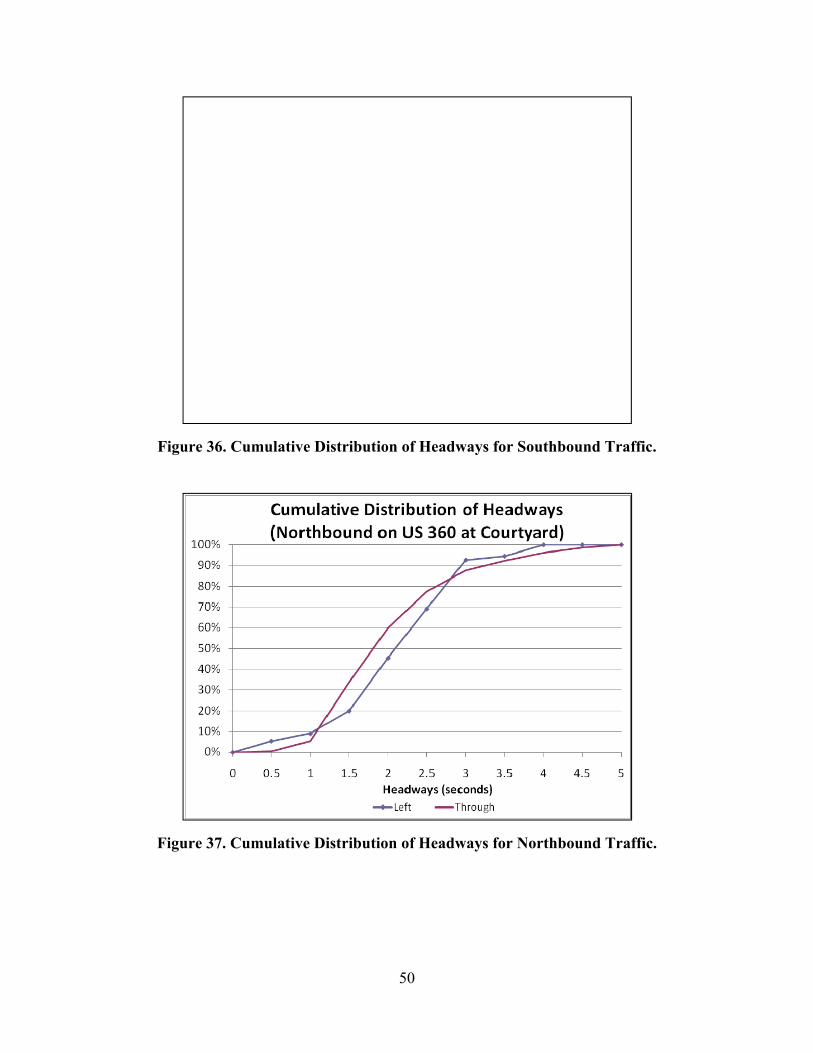
50
Figure 36. Cumulative Distribution of Headways for Southbound Traffic.
Figure 37. Cumulative Distribution of Headways for Northbound Traffic.

51
This analysis shows that the main-street through movements had additional capacity, some of which could be given to the eastbound phase without adversely affecting these phases. Further analysis of flow rates and median headway also supported this conclusion. Based on this analysis, it was concluded that 4 to 6 seconds of green time could be taken away from the two movements and given to the eastbound phase. To be on the conservative side, researchers recommended a 4-second adjustment, followed by a similar analysis to determine the effectiveness of this change. Researchers conducted simple analytical analysis to demonstrate the benefits of proposed changes in timings. This analysis is described below.
Table 9 presents the proposed green splits. The green splits in this table were obtained by taking 4 seconds from main-street through phases and giving this additional time to the eastbound phase. Splits for other phases were not changed. Capacity analysis, using field-observed saturation flow rates for the through main-street through movements, show that all movements have sufficient capacity to handle corresponding demand.
Table 9. Estimated Capacities of the Proposed Timing Plan. Northbound Southbound Eastbound Westbound Left Through Left Through Left+Right Left+Right Phase Time (s) 25 87 18 80 30 15 Lost Time (s) 4 4 4 4 3 3 Effective Green (s) 21 83 14 76 27 12 Saturation Flow (vphpl) 1800 2000 1800 2000 1957 1800 Capacity (vphpl) 252 1107 168 1013 352 144
Extra Capacity due to skip of WB phase 100 100 Total Capacity (vphpl) 252 1207 168 1113 352 144 Critical Lane Demand (vphpl) 82 1163 52 907 287 The next step evaluates the benefit of the proposed timing plan using a simple analytic method. As mentioned previously, eastbound was the only approach at this intersection with operations problems. Thus, the improvement is measured in terms of the effectiveness of queue dissipation at this approach. According to capacity estimate in Table 9, the eastbound approach can serve 29.3 (352/12) vehicles per 5-minute interval. Recall that there was an un-served queue at the beginning of data collection period for this approach (see Figure 34). From the video, the length of this queue was estimated to be 12 vehicles per lane. Assuming that the new timings came into effect at the beginning of the data collection period, Table 10 provides a comparison of the queue dissipation process for existing and proposed timings. This analysis further assumes that:
• the volume of right-turn-on-red (RTOR) is unchanged; and • on average, the flare results in one additional right-turn vehicle serviced during green for
each cycle as compared to the inside lane. This additional service rate is two vehicles per 5-minute analysis provided in Table 10.

52
Table 10. Queue Dissipation Estimation.
5-Minute Service Rate Existing Timing Plan Proposed Timing Plan 25.0 27.0 29.3 31.3
Interval From (min)
To (min)
Demand Remaining Queue Remaining Queue Lane 1 Lane 2 Lane 1 (L) Lane 2 (LR) Lane 1 (L) Lane 2 (LR)
12.0 12.0 12.0 12.0 1 0 5 24 29 11.0 14.0 6.7 9.7 2 5 10 26 30 12.0 17.0 3.3 8.3 3 10 15 25 20 12.0 10.0 0.0 0.0 4 15 20 28 26 15.0 9.0 0.0 0.0 5 20 25 26 27 16.0 9.0 0.0 0.0 6 25 30 16 22 7.0 4.0 0.0 0.0 7 30 35 16 19 0.0 0.0 0.0 0.0 8 35 40 14 19 0.0 0.0 0.0 0.0 9 40 42 3 7 0.0 0.0 0.0 0.0
Note: 1. Observe serviced volume for lane 2 excludes RTOR count. The analysis assumes the same RTOR
counts for the two cases. 2. For both cases, the analysis assumes that one additional right-turn vehicle per cycle uses the green phase
because of the flare at this approach.
Notice that for existing timings, the queue cleared in interval 7, which is very close to the queue dissipation behavior observed from the video. In contrast, proposed timings clear the queue in interval 3, at least 15 minutes earlier than the existing timings. It should be pointed out that this is a very conservative analysis. In reality, maximum queue will be shorter than at present if the new timings were in place at the beginning of evening peak period. As a result, these queues will also dissipate earlier that what the above analysis shows.
CHALLENGES
Preliminary guideline proposed in Chapter 3 made several simplifying assumptions. Application of those guidelines, described in this chapter, revealed that the data collection and analysis task is not simple as assumed. This section summarizes the researchers’ experiences in applying the guideline. The initial recommendation was to collect data for the entire congestion period plus at least 30-minute periods before and after if possible. However, it may not be possible to do so due to resource (trained man power, time, or equipment) constraints or technical difficulties such as weather and lighting conditions. For instance, in one case, the research team used six people to collect data for a three-intersection system. Most agencies do not have such human resources available. Even with this many people, researchers were not able to collect data with desired accuracy (i.e., O-D patterns and demand data). Also, because of lighting issues, researchers could not continue video data collection through the end of peak period.

53
For estimating accurate demand, preliminary guidelines recommended cycle-by-cycle addition of total vehicles serviced and queue growth. However, keeping track of cyclic queue growth was not possible in many cases. With long and rapidly-growing queues, even keeping track of the back of the queue was not possible. The reason was that the dynamic behavior of queue formation made it impossible to define the back of a queue referenced to a point in the signal cycle (i.e., end of green phase). For example, obstructions from an adjacent lane prevented view of a left-turn queue in one case. Another problem is the unavailability of analytical procedures and tools suitable for application to congested signal systems. Most available tools for capacity analysis and signal timing applications were developed for uncongested systems. These can be used in certain cases, as long as the user understands their limitations and takes appropriate measures to account for these limitations. Microscopic simulation programs, which can model congested conditions better, face other types of challenges. For instance, simulation programs cannot model two-way left-turn lanes (TWLTLs) or tapers allowing accurate simulation of lane drops or additions. In addition, they require paths (O-D data) to accurately replicate lane selection and lane changing behavior observe in the field. For example, the researchers faced the following challenges while modeling the closely spaced three-intersection system in College Station.
• Northbound and southbound approaches at the Wellborn Road intersection have TWLTLs in both directions. These TWLTLs served as de facto left-turn bays in the vicinity of the intersections under light demand conditions but serve as full left-turn lanes under heavy left-turn demand. Because there are no other sources or sinks in the vicinity, this traffic behavior does not cause any interference. Thus, the researchers were able to achieve the desired objectives by defining longer left-turn bays. In other cases, use of this technique may not be feasible.
• VISSIM requires definitions of paths. Since O-D information was not collected in the field, researchers initially defined decision points at the upstream ends of all links (as illustrated in Figure 38a). As a result, vehicles were making last-minute path choices, creating significant weaving as illustrated in Figure 38b. Such behavior was not observed in the field. In reality, drivers make lane choice decision dynamically based on traffic conditions. Such dynamic behavior in uncongested and congested conditions cannot be replicated in current simulation models. In the congested situation simulated in this project, drivers were selecting lanes before entering the downstream links. This behavior was replicated by moving the decision points to upstream links and adding estimated O-D information. In most cases, resources do not exist to collect such data, which is a must for closely spaced signals. In such cases, O-D percentages could be estimated using the approach described earlier.

54
a. Before Obtaining Turning Decision.
b. After Obtaining Turning Decision.
Figure 38. Routing Decision in VISSIM.
Routing Decision Point
1
2
Routing Decision Point
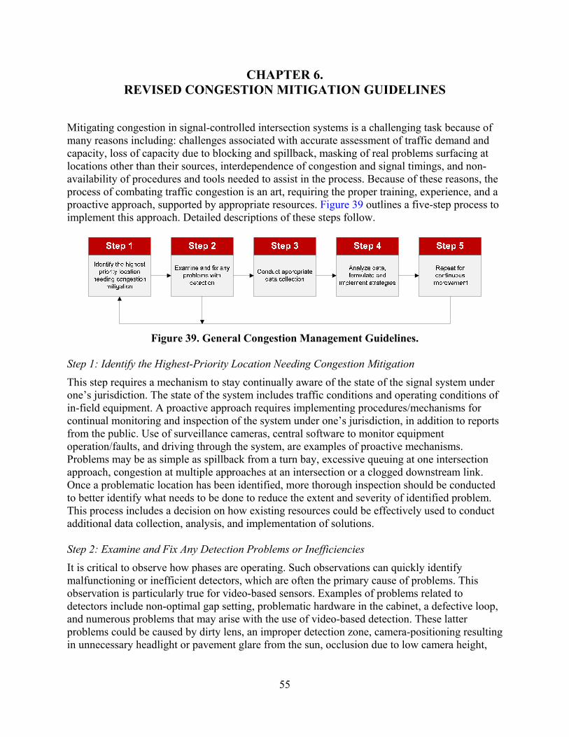
55
CHAPTER 6. REVISED CONGESTION MITIGATION GUIDELINES
Mitigating congestion in signal-controlled intersection systems is a challenging task because of many reasons including: challenges associated with accurate assessment of traffic demand and capacity, loss of capacity due to blocking and spillback, masking of real problems surfacing at locations other than their sources, interdependence of congestion and signal timings, and non-availability of procedures and tools needed to assist in the process. Because of these reasons, the process of combating traffic congestion is an art, requiring the proper training, experience, and a proactive approach, supported by appropriate resources. Figure 39 outlines a five-step process to implement this approach. Detailed descriptions of these steps follow.
Figure 39. General Congestion Management Guidelines.
Step 1: Identify the Highest-Priority Location Needing Congestion Mitigation This step requires a mechanism to stay continually aware of the state of the signal system under one’s jurisdiction. The state of the system includes traffic conditions and operating conditions of in-field equipment. A proactive approach requires implementing procedures/mechanisms for continual monitoring and inspection of the system under one’s jurisdiction, in addition to reports from the public. Use of surveillance cameras, central software to monitor equipment operation/faults, and driving through the system, are examples of proactive mechanisms. Problems may be as simple as spillback from a turn bay, excessive queuing at one intersection approach, congestion at multiple approaches at an intersection or a clogged downstream link. Once a problematic location has been identified, more thorough inspection should be conducted to better identify what needs to be done to reduce the extent and severity of identified problem. This process includes a decision on how existing resources could be effectively used to conduct additional data collection, analysis, and implementation of solutions. Step 2: Examine and Fix Any Detection Problems or Inefficiencies It is critical to observe how phases are operating. Such observations can quickly identify malfunctioning or inefficient detectors, which are often the primary cause of problems. This observation is particularly true for video-based sensors. Examples of problems related to detectors include non-optimal gap setting, problematic hardware in the cabinet, a defective loop, and numerous problems that may arise with the use of video-based detection. These latter problems could be caused by dirty lens, an improper detection zone, camera-positioning resulting in unnecessary headlight or pavement glare from the sun, occlusion due to low camera height,

56
and differences in algorithms for day and nighttime operations. Ideally, the detection system should be snappy, while providing service to all existing demand for a phase. Step 3: Collect Data
Based on assessment from Step 1, develop a data collection plan and conduct actual data collection. The data collection plan may be as simple as field observation by an experienced person or very detailed data collection requiring multiple personnel per intersection in the study area. In case it is not possible to collect all data during the same time period, include measures to properly fusing data collected over multiple days and time periods. To understand where congestion starts, how it spreads, and how long it lasts, it is desirable to collect data for the entire congestion period, plus some time before and after, if possible. In many cases, resource or technical constraints will not permit such detailed data collection. In those cases, do the best you can to understand behavior of queues. Also, collect demand data with as much accuracy as possible. To do that, select an appropriate interval (i.e., 5 to 15 minutes), count the number of vehicles serviced during that interval, and assess how queue changes during this time. Add serviced volume to queue-change to estimate demand. Step 4: Analyze Data, Formulate, and Implement Strategies Analyze the data, determine what needs to be done to fix the problem, and implement changes in signal timings. The fix may be as simple as on-the-spot re-allocation of time between conflicting phases or changes in the offset at a traffic signal. In more complicated cases, data will have to be further processed in the office with the use of available tools. In using the tools, ensure that steps are taken to counter the limitations of tools used. Make sure that appropriate signal timing objectives are appropriate for the conditions at hand. During light to moderate conditions, the objective of timing traffic signals is to minimize delay, minimize stops, or maximize progression. However, during heavy conditions, these objectives cannot be achieved. Under those circumstances, consider throughput maximization and management of queues to prevent spill back and blocking, especially their impact on bays. As demonstrated earlier, a left-turn and through movement being fed traffic from a single upstream lane may not provide full ideal capacities assumed by intersection capacity analysis procedures. Research in this projects shows that the throughput capacities of these movements depends on turn-bay length, number of lanes in the bay, traffic distribution, and signal timings. The researchers recommend that such movements should be treated as a single lane groups. As an example, consider an approach with three full lanes feeding traffic to one left-turn bay and one right-turn bay. In this case, the analyst should consider using the following three lane groups:
a. left-turn bay and adjacent through lane as one lane group, b. through lane in the middle as one group, and c. right-turn bay and adjacent through lane as the third group.
Actual volume counts for movements at an approach such as that identified above can be
used to estimate the capacities of these lane groups as long as there is constant demand. Once assessment has been completed, specific tactics can be used to tackle identified problems. These tactics may include:

57
• addressing downstream bottleneck if queues prevent full utilization (starvation) of upstream green phases,
• serving heavy movements twice per cycle, • optimizing green splits, • finding the most appropriate cycle length, • minimizing effects of pedestrians, • balancing queues on conflicting approaches, • minimizing queue damage, • appropriately selecting phasing sequences, • selecting appropriate max times, and • minimizing adverse effects of transitioning in coordinated systems.
Another approach is the use of a single controller for multiple intersections, especially
those closely-spaced. Such operation allows actuated operation to handle variations in demand, while maintaining coordination between the intersections at all times. However, this option should be considered only after careful consideration of detection design and phasing. Step 5: Repeat the Process Implement revised signal timings and repeat Step 1. You may encounter one of the following scenarios:
• the problem is completely solved, • the problem has shifted to another location with more or less severe impact, • congestion is reduced but is still there, or • you cannot tell the difference.
If the problem shifted to a different location, consider a more refined system-based
approach. However, it may or may not be able to completely eliminate congestion, especially if the demand is truly more than capacity. In that case, you may need to set priorities and tweak control so that congestion is pushed away from critical locations to other locations. For instance, in dealing with interchanges, make sure that queues are prevented from compromising the safety of the freeway exit or main lane traffic. In some cases, all you may be able to do within the existing constraints is to reduce the impacts of congestion. In such cases, you are successful if the above process allowed you to reduce the severity and duration of congestion.


59
REFERENCES
1. National Traffic Signal Report Card: Executive Summary 2007. National Transportation
Operations Coalition. http://www.ite.org/reportcard/NTSRC%20Exec%20Summary%20final.pdf. Accessed February 18, 2008.
2. Gazis D. and R. Potts. The Oversaturated Intersection. In Proceedings of the 2nd International Symposium on Traffic Theory. pp. 221–237. 1963.
3. D’Ans, G. and D. Gazis. Optimal Control of Oversaturated Store-and-Forward Transportation Networks. Transportation Science. Vol. 10. No. 1. pp. 1–19. 1976.
4. Rahmann, W. Storage/Output Design of Traffic Signals. Australian Road Research, Vol.5. No.1. pp. 38–43. 1973.
5. Pignataro, L., W. McShane, K. Crowley, and T. Casey. Traffic Control in Oversaturated Street Networks. NCHRP Report 194, Transportation Research Board. Washington, D.C. 1978.
6. Lee B., K Crowley, and L. Pignataro. Better Use of Signals Under Oversaturated Flows. Transportation Research Board. Special Report 153. Washington, D.C. pp. 60–72. 1975.
7. Lieberman, E., Messer, C.J. Internal Metering Policy for Oversaturated Networks. Report TR-238, KLD Associates, New York, March 1990.
8. Gal-Tzur, A., D. Mahalel, and J. Prashker. Signal Design for Congested Networks Based on Metering. Transportation Research Record 1398. pp. 111–118. 1993.
9. Choi, B-K, Adaptive Signal Control for Oversaturated Arterials. Ph.D., Thesis, Polytechnic University, New York, 1997.
10. Lieberman E. and J. Chang. Optimizing Traffic Signal Timing Through Network Decomposition. Transportation Research Record 1925. pp. 167–175. 2005.
11. Kim Y. Development of Optimization Models for Signalized Intersections During Oversaturated Conditions. Ph.D. Thesis, Texas A&M University, College Station, Texas 1990.
12. Kim Y. and C. Messer. Traffic Signal Timing Models for Oversaturated Signalized Interchanges. Interim Report FHWA/TX-92/1148-2, Texas Transportation Institute. College Station, TX, January 1992.
13. Chaudhary, N. and K. Balke. Real-Time Coordinated-Actuated Traffic Control During Congested Conditions. Report FHWA/TX-99/1288-S. Texas Transportation Institute. December 1997.
14. Messer, C. J. Simulation Studies of Traffic Operations at Oversaturated, Closely Spaced Signalized Intersections. Transportation Research Record 1646. pp. 115–123. 1998.
15. Messer, C.J. Extension and Application of Prosser-Dunne Model to Traffic Operation Analysis of Oversaturated, Closely-Spaced Signalized Intersections. Transportation Research Record 1646. pp. 106–114, 1998.
60
16. Chaudhary N. and C.-L. Chu. Guidelines for Timing and Coordinating Diamond Interchanges with Adjacent Traffic Signals. Report No. TX-00/4913-2, Texas Transportation Institute. College Station, Texas, November 2000.
17. Chaudhary, N., C.-L. Chu, K. Balke, and V. Kovvali. Coordination of Diamond Interchanges with Adjacent Traffic Signals. Report No. TX-00/4913-1, Texas Transportation Institute. College Station, Texas, Oct. 2000.
18. Webster, F.V. and B.M. Cobbe. Traffic Signals, Road Research, Technical Paper No. 56, Her Majesty’s Stationery Office, London, England, 1966.
19. Chu, C.-L. and N. Chaudhary. Coordination of Diamond Interchange with Adjacent Traffic Signals. 2005 Annual Transportation Research Board Meeting CD ROM, January 2005.
20. Abu-Lebdeh, Ghassan and R. Benekohal. Design and Evaluation of Dynamic Traffic Management Strategies for Congested Conditions. Transportation Research – A. Vol. 37. No. 2. pp. 109–127. 2003.
21. Liu, H. and K. Masao. An Approach on Network Traffic Signal Control under the Real-Time and Oversaturated Flow Condition. In 80th Annual Transportation Research Board Meeting CD ROM. Washington, D.C., January 2001.
22. Ahn G-H, and R. Machemehl. Methodology for Traffic Signal Timing in Oversaturated Arterial Networks. Report SWUTC/98/465510-1, University of Texas, Austin, Texas, October 1997.
23. Abu-Lebdeh G. and R. Benekohal. Signal Coordination and Arterial Capacity in Oversaturated Conditions. Transportation Research Record 1727. pp. 68–76. 2000.
24. Khatib Z., A. Abdel-Rahim, G. Judd, and K. Jagarapu. Actuated Coordinated Signal System, Phase I-Oversaturated Conditions, Phase II-Cycle-by-Cycle Analysis. Final Report N01-20, National Institute for Advanced Transportation Technology. University of Idaho. November 2001.
25. Girianna, M. and R. Benekohal. Dynamic Signal Coordination for Networks with Oversaturated Intersections. Transportation Research Record 1811. pp. 122–130. 2002.
26. Herrick, C. and C. Messer. Strategies for Improving Traffic Operations at Oversaturated Diamond Interchanges. Final Report FHWA/TX-92/1148-4F. Texas Transportation Institute. College Station, Texas, March 1992.
27. Denny, R., L. Head, and K. Spencer. Signal Timing under Saturated Conditions. Final Report FHWA-HOP-09-008, Federal Highway Administration. Washington, D.C., November 2008.
28. Click S. Retiming of NC 54 at I-40 and Farrington Road in Durham, NC: A Case Study in Oversaturated Control. Presented at January 2007 Transportation Research Board Workshop on Operating Traffic Signal Systems in Oversaturated Conditions, January 21, 2007.
29. Sabra Z. Strategies to Mitigate Gridlock on High Volume Arterials in Sacramento County, CA. Presented at January 2007 Transportation Research Board Workshop on Operating Traffic Signal Systems in Oversaturated Conditions, January 21, 2007.

61
30. Chamberlin, R. Ongoing Efforts to Coordinate and Oversaturated Corridor in Lebanon, New Hampshire. Presented at January 2007 Transportation Research Board Workshop on Operating Traffic Signal Systems in Oversaturated Conditions, January 21, 2007.
31. De Camp G. A Michigan’s Secret for Operating Traffic Signals during Oversaturation. Presented at January 2007 Transportation Research Board Workshop on Operating Traffic Signal Systems in Oversaturated Conditions, January 21, 2007.
32. Nelson, E. Timing Strategies for Managing Oversaturation in Harris County. Presented at January 2007 Transportation Research Board Workshop on Operating Traffic Signal Systems in Oversaturated Conditions, January 21, 2007.
33. Bathelder, J.H., M. Golenberg, J.A. Howard, and H.S. Levinson. Simplified Procedures for Evaluating Low-Cost TSM Projects. NCHRP Report 263. Transportation Research Board. Washington, D.C. 1983.
34. Koepke, F.J. and H.S. Levinson. Access Management Guidelines for Activity Centers. NCHRP Report 348. Transportation Research Board. Washington, D.C. 1992.
35. Gluck, J., H.S. Levinson, and V. Stover. Impacts of Access Management Techniques. NCHRP Report 420. Transportation Research Board. Washington, D.C. 1999.
36. Zhang, W. Synthesis of the Median U-Turn Intersection Treatment, Safety, and Operational Benefits. FHWA-HRT-07-033. FHWA. Washington, D.C. 2007.
37. Lindley, J.A. Quantification of Urban Freeway Congestion and Analysis of Remedial Measures. Report FHWA/RD-87/052. FHWA, U.S. Department of Transportation, 1986.
38. Levinson, S. and T. Lomax. Developing a Travel Time Congestion Index. Transportation Research Record 1564. pp. 1–10. 1996.
39. Vaziri, M. Development of Highway Congestion Index with Fuzzy Set Models. Transportation Research Record 1802. pp. 16–22. 2002.
40. Hamad, K and S. Kikuchi. Developing a Measure of Traffic Congestion: Fuzzy Inference Approach. Transportation Research Record 1802. pp. 77-85. 2002.
41. Appelbaum, A. Mayor Bloomberg Says NYC Traffic Congestion is Good. http://www.streetsblog.org/2006/08/02/mayor-bloomberg-says-nycs-traffic-congestion-is-good/. Accessed March 2, 2007.
42. Taylor, B. Rethinking Traffic Congestion. Access. Vol. 21. pp. 8–16. 2002.
43. Urbanik, T. Oversaturation: What Do We Really Know? Presented at January 2007 Transportation Research Board Workshop on Operating Traffic Signal Systems in Oversaturated Conditions, January 21, 2007.
44. Messer, C.J. and D. B. Fambro. Effects of Signal Phasing and Length of Left-Turn Bay on Capacity. Transportation Research Record 644. pp. 95-101. 1977.
45. VISSIM 5.10 User Manual. PTV AG. Karlsruhe, Germany. 2008.
46. Highway Capacity Manual 2000. Transportation Research Board, Washington, D.C. 2000.


63
APPENDIX A: QUESTIONNAIRE


65
TxDOT Project No. 0-5998
EVALUATION OF BEST PRACTICES FOR CONTROLLING SIGNAL SYSTEMS DURING OVERSATURATED CONDITIONS.
State of the Practice Assessment
TTI, in cooperation with TxDOT’s Research and Technology Implementation Office, is conducting a research project to evaluate the best practices for controlling signal systems during oversaturated conditions. The objective of the project is to develop guidelines for eliminating or mitigating the effects of oversaturated traffic signals. As part of this project, we are contacting TxDOT Districts and other agencies to determine and document current practices for dealing with oversaturated conditions at signalized intersections. Contact Information
Please provide your name, telephone number, and e-mail address so that we can contact you in the future about your responses. Name: Title: Agency/TxDOT District: Telephone: E-mail:
General
How many signalized intersections does your agency maintain?
Of all the signalized intersections your agency maintains, what percentage are …. Isolated Coordinated
Of all the signalized intersections your agency maintains, what percentage would you
estimate to be …. Traditional four-legged intersection Three-legged intersections Diamond interchanges Other
How many coordinated signal systems does your agency maintain?

66
Characterization of Oversaturation
Which of the following problems do you typically see at intersections that are congested or oversaturated? (Check all that apply)
Traffic queue unable to clear during a single cycle (cycle failure) _____ Traffic queue unable to clear within ___ consecutive cycles Phases not being fully utilized because queues prevent or block traffic from
reaching lane or intersection Extremely long queue(s) on one or more approaches Unable to obtain large progression bands through multiple intersections Low total throughput through the intersection Spillback of long queue from a downstream intersection preventing traffic to
move through the current intersection Other (please describe):
_________________________________________________________________________________________________________________________________________________________________________________________________________
What percentage of intersections routinely experience oversaturated conditions? _____
What percentage of intersection occasionally experience oversaturated conditions? _____
Are more of your oversaturated intersections isolated or part of a coordinated traffic signals
system?
Isolated Coordinated About the same
Management Objectives for Oversaturated Conditions
In trying to develop a “fix” for a congestion problem at an isolated intersection, what are your primary and secondary objectives in setting signal timings?
Minimize total intersection delay Minimize time spent waiting in the queue before clearing the intersection Minimize the total number of stops at the intersection Minimize the number of cycles required to clear a vehicles through the
intersection Maximize productivity/throughput (total volume) through the intersection Avoid spillback from congested approach from blocking upstream intersection Limit queues causing “starvation” to under-utilized phases Minimize duration for which an intersection/approach is oversaturated Provide equitable service to all movements at the intersection

67
Other (please specify):
In trying to develop a “fix” for a congestion problem at an intersection in a coordinated system, what are your primary and secondary objectives in setting signal timings?
Minimize total intersection delay Minimize time spent waiting in the queue before clearing the intersection Minimize the total number of stops at the intersection Minimize the number of cycles required to clear a vehicles through the
intersection Maximize progression through the intersection Maximize progression through the intersection in the peak direction only Maximize progression away from the intersection Maximize productivity/throughput (total volume) through the intersection Avoid spillback from congested approach from blocking upstream intersection Limit queues causing “starvation” to under-utilized phases Minimize duration for which an intersection/approach is oversaturated Maintain travel-time reliability (or consistency) through the intersection Provide equitable service to movements at the intersection by adjusting phase
times _____ Provide equitable service to movements at a upstream signal by adjusting offsets Other (please specify):
Does your management objectives/priority change if the congested approach affects or is
affected by a diamond (or other type of) interchange? Yes No
If YES, how? _____________________________________________________________________________________________________________________________________________________________________________________________________________________________________________________________________________________________________________________________________________________________________________________________________________________________________________________________________________________________________________________________________________________________________________________________________________________________________________________________________________________________________________________

68
5.
Stra
tegi
es fo
r M
anag
ing
Ove
rsat
urat
ed T
raff
ic C
ondi
tions
5.
1. L
iste
d be
low
are
seve
ral c
andi
date
stra
tegi
es fo
r add
ress
ing
over
satu
ratio
n at
sign
aliz
ed in
ters
ectio
ns.
If y
ou h
ave
used
one
or
mor
e of
thes
e st
rate
gies
in y
our a
genc
y, p
leas
e ra
te it
s ove
rall
succ
essf
ulne
ss (t
otal
ly, m
argi
nally
, or u
nsuc
cess
ful)
at
addr
essi
ng th
e ov
ersa
tura
tion
prob
lem
. If
you
hav
e no
t use
d th
e st
rate
gy, p
leas
e ch
eck
“Hav
e N
ot T
ried.
”
St
rate
gy
Tota
lly
Succ
essf
ulM
argi
nally
Su
cces
sful
Uns
ucce
ssfu
lH
ave
Not
Tr
ied
a.
Elim
inat
e or
pro
hibi
t mov
emen
t or p
hase
at a
n in
ters
ectio
n
b.
Sk
ip o
ne o
r mor
e ph
ases
in a
ltern
ate
cycl
es
c.
Act
ivat
e ph
ase
or “
doub
le c
ycle
” so
me
phas
es d
urin
g a
sing
le c
ycle
d.
C
hang
e se
quen
cing
of p
hasin
g
e.
El
imin
ate
or p
rohi
bit p
edes
trian
mov
emen
ts o
r pha
ses
f. U
se d
etec
tor t
o ho
ld p
hase
to c
lear
que
ue (s
imila
r to
“flu
sh o
f ram
p m
eter
”)
g.
Incr
ease
tota
l cyc
le le
ngth
of s
igna
l
h.
Dec
reas
e to
tal c
ycle
leng
th o
f sig
nal
i. U
se a
n up
stre
am tr
affic
sign
al o
r app
roac
h to
stor
e ex
cess
dem
and
and/
or li
mit
flow
to
dow
nstre
am a
ppro
ach
(i.e.
, met
er d
eman
d)
j. R
educ
e th
e du
ratio
n of
cro
ss-s
treet
pha
ses t
o le
ss th
an o
ptim
al to
pro
vide
mor
e gr
een
to
the
mai
n st
reet
k.
Res
trict
upp
er c
ycle
leng
th to
pre
vent
a q
ueue
reac
hing
an
upst
ream
sign
al
l. C
hang
e fr
om tw
o-w
ay to
one
-way
pro
gres
sion
(us
ually
in p
eak
dire
ctio
n) to
pro
vide
pr
efer
entia
l tre
atm
ent t
o di
rect
ion
of c
onge
stio
n
m
. M
axim
ize
prog
ress
ion
away
from
con
gest
ed a
ppro
ach
n.
Hol
d m
ain
stre
et w
ith g
reen
inte
rval
for a
n ex
tend
ed ti
me
(e.g
., 4
to 5
min
utes
) to
“flu
sh”
dem
and
from
syst
em
o.
Dro
p in
ters
ectio
n fr
om c
oord
inat
ion
and
run
in is
olat
ed m
ode

69
St
rate
gy
Tota
lly
Succ
essf
ulM
argi
nally
Su
cces
sful
Uns
ucce
ssfu
lH
ave
Not
Tr
ied
p.
Incr
ease
bay
leng
ths t
o re
duce
und
er-u
tiliz
atio
n of
pha
ses
q.
Incr
ease
the
num
ber o
f lan
es in
a tu
rn-b
ay
r. In
crea
se th
e to
tal n
umbe
r of l
anes
on
an a
ppro
ach
thro
ugh
the
inte
rsec
tion
s. U
se sp
ecia
l tur
n la
nes (
such
as j
ug h
andl
es o
r mid
-blo
ck U
-turn
s) to
rem
ove
dem
and
of
left-
turn
pha
ses
t. O
ther
(Ple
ase
Spec
ify):
u.
Oth
er (P
leas
e Sp
ecify
):
v.
O
ther
(Ple
ase
Spec
ify):

70
5.2.
Lis
ted
belo
w a
re se
vera
l can
dida
te st
rate
gies
that
we
have
iden
tifie
d fo
r add
ress
ing
over
satu
ratio
n at
sign
al in
ters
ectio
ns.
Plea
se in
dica
te w
heth
er, i
n yo
ur o
pini
on, y
ou th
ink
the
stra
tegy
is v
iabl
e, n
ot v
iabl
e, o
r unc
erta
in fo
r use
in y
our d
istri
ct.
A
viab
le o
ptio
n w
ould
be
one
that
you
wou
ld c
onsi
der i
mpl
emen
ting
(whe
ther
or n
ot y
ou h
ave
alre
ady
tried
it).
An
unvi
able
op
tion
is o
ne th
at fo
r wha
teve
r rea
son
(unp
opul
ar, u
nsaf
e, li
abili
ty c
once
rns,
etc.
) you
wou
ld n
ot e
ven
cons
ider
ing
impl
emen
ting
in y
our d
istri
ct.
St
rate
gy V
iabl
e
Not
via
ble
Unc
erta
in
a.
Elim
inat
e or
pro
hibi
t mov
emen
t or p
hase
at a
n in
ters
ectio
n b.
Sk
ip o
ne o
r mor
e ph
ases
in a
ltern
ate
cycl
es
c.
Act
ivat
e ph
ase
or “
doub
le c
ycle
” so
me
phas
es d
urin
g a
sing
le c
ycle
d.
C
hang
e se
quen
cing
of p
hasin
g e.
El
imin
ate
or p
rohi
bit p
edes
trian
mov
emen
ts o
r pha
ses
f. U
se d
etec
tor t
o ho
ld p
hase
to c
lear
que
ue (s
imila
r to
“flu
sh o
f ram
p m
eter
”)
g.
Incr
ease
tota
l cyc
le le
ngth
of s
igna
l h.
D
ecre
ase
tota
l cyc
le le
ngth
of s
igna
l i.
Use
an
upst
ream
traf
fic si
gnal
or a
ppro
ach
to st
ore
exce
ss d
eman
d an
d/or
lim
it flo
w to
do
wns
tream
app
roac
h (i.
e., m
eter
dem
and)
j. R
educ
e th
e du
ratio
n cr
oss-
stre
et p
hase
s to
less
than
opt
imal
to p
rovi
de m
ore
gree
n to
the
mai
n st
reet
k.
Res
trict
upp
er c
ycle
leng
th to
rest
rict c
ritic
al a
ppro
ach
queu
es re
achi
ng u
pstre
am si
gnal
l.
Cha
nge
from
two-
way
to o
ne-w
ay p
rogr
essi
on (u
sual
ly in
pea
k di
rect
ion)
to p
rovi
de
pref
eren
tial t
reat
men
t to
dire
ctio
n of
con
gest
ion
m
. M
axim
ize
prog
ress
ion
away
from
con
gest
ed a
ppro
ach
n.
Hol
d m
ain
stre
et w
ith g
reen
inte
rval
for a
n ex
tend
ed ti
me
(e.g
., 4
to 5
min
utes
) to
“flu
sh”
dem
and
from
syst
em
o.
D
rop
inte
rsec
tion
from
coo
rdin
atio
n an
d ru
n in
isol
ated
mod
e p.
In
crea
se b
ay le
ngth
s to
redu
ce u
nder
-util
izat
ion
of p
hase
s q.
In
crea
se th
e nu
mbe
r of l
anes
in a
turn
-bay
r.
Incr
ease
the
tota
l num
ber o
f lan
es o
n an
app
roac
h th
roug
h th
e in
ters
ectio
n s.
Use
spec
ial t
urn
lane
s (su
ch a
s jug
han
dles
or m
id-b
lock
U-tu
rns)
to re
mov
e de
man
d of
le
ft-tu
rn p
hase
s
t. O
ther
(Ple
ase
Spec
ify):
u.
O
ther
(Ple
ase
Spec
ify):
v.
O
ther
(Ple
ase
Spec
ify):

71
6. Potential Study Locations As part of this research project, we are looking for candidate locations where we can field test some of the strategies listed above. If you have locations in your agency that you think would be suitable study sites and you would be interested in working with us to test some of these strategies, please identify those locations and provide brief descriptions of problems observed at these sites. Location: Number of Signals in the System: Description of Problem: Location: Number of Signals in the System: Description of Problem: Location: Number of Signals in the System: Description of Problem:


73
APPENDIX B: SUMMARY OF RESPONSES TO QUESTIONNAIRE


75
Signal In
form
ation So
rted
from
Smallest to Largest
Num
ber of Signa
ls
# Sigs
% isolated
% Coo
rdinated
4‐leg
3‐Leg
Diamon
dOther
# Co
ordina
ted
System
s Respo
nden
t
2 59
85
15
4
Gordo
n harked
(Brownw
ood)
a 70
30
70
79
.00
3 18
5 Ra
mana Ch
innakotla
d 70
4
96
4 80
16
John
Black, Frisco (M
oved
to Lew
isville since
then
) 8
80
86
14
90
1 9
2
Roy Wright (Abilene
)
1 94
50
50
50
10
40
2 Arm
ando
Sanchez and
Bob
by Rod
riguez
(Lared
o/Del Rio)
7 10
0 56
44
85
5
5 5
6 Herbe
rt Bickley (Lufkin)
4
120
56
44
65
17
10
8 10
Larry Co
lclasure (W
aco)
f 12
3 5
95
85
5 10
1 Dave Carter/Rob
ert S
aylor, City
of
Richardson
3
478
77
23
65
7 28
11
David Smith
(San
Anton
io)
5 48
5 65
35
60
10
30
170
J.D. G
ore (Fort W
orth)
b 80
0 30
70
70
20
5
30
0 tie
d to
central
Eric Nelson, Harris Co
unty 713
‐881
‐331
5, left
since survey
c 85
0 80
10
10
5
95
50
Austin
, Ali Mozdb
ar
y 11
50
38
62
49
38
13
55
John
Frieb
ele, W
ilbur Smith
6
1200
33
67
75
8
17
70
Dou
g Va
nover (Hou
ston
)
e
1292
3
97
84
4 10
2
75
Mark Titus, City
of D
allas
9 62
16
15
85
3730
12
43
622
622
104
(Closed loop
) Hen
ry W
ickes (Signal and
Radio Ope
ratio
ns)
x N/A
Jody
Sho
rt/Kelly Parma, Lee
Engineering
Not
e: T
xDO
T re
spon
ses a
re la
bele
d 1
thro
ugh
9, p
ublic
age
ncy
resp
onse
s are
labe
led
a th
roug
h f,
and
cons
ulta
nt re
spon
ses a
re la
bele
d x
and
y.

76
Oversaturation Ch
aracterized by
a
b c
d e
f g
% In
tersection
s Facing
Con
gestion
Oversaturation Mostly in
Single
Cycle
Failu
re
Consecutive
CFs
Phase
Capa
city
Lost due
to
Blocking
Long
Qs on
on
e or
more
App
roache
s
Cann
ot get
Accep
table
Progression
Band
s
Low
Through‐
put
Spillba
ck
from
Dow
nstream
Intersection
Routinely
Occasiona
l Isolated
Co
ordina
ted
Abo
ut
Same
1 x
3 to 4
x x
x
x 43
13
x
2 x
x
10
5
x
3 x
2
x
x
<10
20
x 4
x
x
x
x 15
25
x
5 x
2 to 3
x
x 10
20
6 x
3 x
x x
x x
65
15
x
7
x x
x x
x 5
10
x
8
x
0
0
9 x
3 x
x x
x
a
x 2
x x
x x
x 15
20
x
b
3 x
x
5 10
x
c x
x
x x
x
5 15
x
d x
2
15
25
x
e
x
50
80
x
f x
2 x
x
15
50
x
x
x
x x
x 10
14
x
y x
x
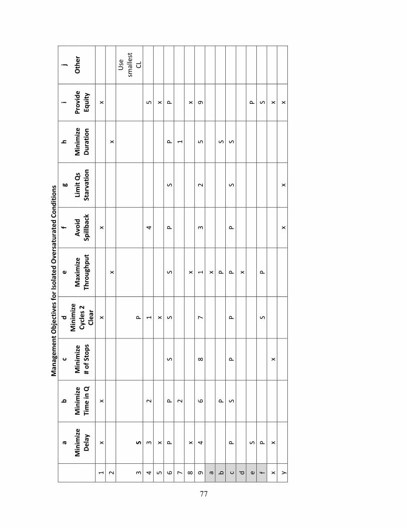
77
Man
agem
ent Objectives for Isolated
Oversaturated
Con
dition
s
a b
c d
e f
g h
i j
Minim
ize
Delay
Minim
ize
Time in Q
Minim
ize
# of Stops
Minim
ize
Cycles 2
Clear
Maxim
ize
Throug
hput
Avoid
Spillba
ck
Limit Qs
Starvation
Minim
ize
Duration
Provide
Equity
Other
1 x
x
x
x
x
2
x
x
3 S
P
Use
smallest
CL
4 3
2
1
4
5
5
x
x
x
6 P
P S
S S
P S
P P
7
2
1
8 x
x
x
9
4 6
8 7
1 3
2 5
9
a
x
b
P
P
S
c P
S P
P P
P S
S
d
x
e S
P
f
P
S
P
S
x x
x
x
y
x
x
x

78
Man
agem
ent Objectives for Co
ordina
ted System
Oversaturated
Con
dition
s
Minimize Delay
Minimize Time in Q
Minimize # of Stops
Minimize Cycles 2 Clear
Maximize Progression Through
Intersection
Maximize Progression In peak
Dir Only
Maximize Progression Away from Intersection
Maximize Throughput
Avoid Congested Approach from
Blocking Upstream Intersection
Limit Qs to Prevent Starvation to
Underutilized Phases
Minimize Duration
Maintain Travel Time Reliability
Provide Equity to Movements at Intersection
Provide Equity at Upstream Intersection
1 x
x x
x x
x
x x
x
2
1
2
3
4
2
1
3
5
x
x x
x
x
6
P S
P S
P P
S S
P S
S S
P P
7
1
2
8
x
x
x x
9 4
6 8
7
1 3
2 5
9 a
x
x
b
P
S
P P
S
c
S S
S
P P
P P
P S
S P
S P
d
S
P
e
S
P
f P
P
S
x
x
x x
x
x
y
x
x

79
Strategies fo
r Man
aging Oversaturated
Traffic Con
dition
s
Stra
tegy
* T
otal
ly
Succ
essf
ul
Mar
gina
lly
Succ
essf
ul
Uns
ucce
ssfu
lH
ave
Not
Tri
ed
Via
ble
Not
V
iabl
e U
ncer
tain
a 3cd
8efxy
124567ab
69acdefxy
12345b
7
b cd
5befxy
3
124678ab
4579abcdefxy
3
126
c 35cd
befx
124678ay
2345679abcdefxy
1
d 35cf
24678abdex
y
1
2345679abcdefxy
1
e
e
ad
12345678bcfxy 26aex
1357bcdfy
49
f
347abcd
12568efxy
234679acdex
15bfy
g 3
1245678cdefxy
a
2345679abcdefxy
1
h 3
2568cdefxy
14a
7
345679abcdefxy
12
i 35d
cefxy
4a
12678b
345679abcdefxy
12
j
23457bcdefxy
a
168
2345679abcdefx
y
1
k d
45cex
123678abfy
345679acdefx
12by
l 3
2678efy
1
5acdx
12345679bcefxy
ad
m
3bd
25e
14678acfxy
235679abcde
4
1fxy
n
34de
1235678abcfxy 467dex
35acf
129bcy
o 3
456dfxy
ac
1278e
345679abcdefxy
1
p 4de
26fy
a
13578bcx
34569abcdefxy
2
17
q 358bdy
246cef
17ax
34569abcdefxy
2
17
r 458bd
126cefy
137ax
134569bcdefxy
2a
7
s d
c
123567abcefxy 469bcdef
2a
1357xy
* Se
e ta
ble
on th
e ne
xt p
age
for d
escr
iptio
ns o
f stra
tegi
es.

80
Strategy Description
s
Stra
tegy
Str
ateg
y D
escr
iptio
n
a El
imin
ate
or p
rohi
bit m
ovem
ent o
r pha
se a
t an
inte
rsec
tion
b Sk
ip o
ne o
r mor
e ph
ases
in a
ltern
ate
cycl
es
c A
ctiv
ate
phas
e or
“do
uble
cyc
le”
som
e ph
ases
dur
ing
a si
ngle
cyc
le
d C
hang
e se
quen
cing
of p
hasin
g
e El
imin
ate
or p
rohi
bit p
edes
trian
mov
emen
ts o
r pha
ses
f U
se d
etec
tor t
o ho
ld p
hase
to c
lear
que
ue (s
imila
r to
“flu
sh o
f ram
p m
eter
”)
g In
crea
se to
tal c
ycle
leng
th o
f sig
nal
h D
ecre
ase
tota
l cyc
le le
ngth
of s
igna
l
i U
se a
n up
stre
am tr
affic
sign
al o
r app
roac
h to
stor
e ex
cess
dem
and
and/
or li
mit
flow
to d
owns
tream
app
roac
h (i.
e., m
eter
dem
and)
j R
educ
e th
e du
ratio
n of
cro
ss-s
treet
pha
ses t
o le
ss th
an o
ptim
al to
pro
vide
mor
e gr
een
to th
e m
ain
stre
et
k R
estri
ct u
pper
cyc
le le
ngth
to p
reve
nt a
que
ue re
achi
ng a
n up
stre
am si
gnal
l C
hang
e fr
om tw
o-w
ay to
one
-way
pro
gres
sion
(usu
ally
in p
eak
dire
ctio
n) to
pro
vide
pre
fere
ntia
l tre
atm
ent t
o di
rect
ion
of c
onge
stio
n
m
Max
imiz
e pr
ogre
ssio
n aw
ay fr
om c
onge
sted
app
roac
h
n H
old
mai
n st
reet
with
gre
en in
terv
al fo
r an
exte
nded
tim
e (e
.g.,
4 to
5 m
inut
es) t
o “f
lush
” de
man
d fr
om sy
stem
o D
rop
inte
rsec
tion
from
coo
rdin
atio
n an
d ru
n in
isol
ated
mod
e
p In
crea
se b
ay le
ngth
s to
redu
ce u
nder
-util
izat
ion
of p
hase
s
q In
crea
se th
e nu
mbe
r of l
anes
in a
turn
-bay
r In
crea
se th
e to
tal n
umbe
r of l
anes
on
an a
ppro
ach
thro
ugh
the
inte
rsec
tion
s U
se sp
ecia
l tur
n la
nes (
such
as j
ug h
andl
es o
r mid
-blo
ck U
-turn
s) to
rem
ove
dem
and
of le
ft-tu
rn p
hase
s

81
Potential Study
Locations
Location
/System
Num
ber
in System
Description
IH35
and
Calton Ro
ad, Lared
o 1
Diamon
d with
intersectio
ns to
west (25
0') and
east (300'), with
heavy truck traffic.
Oversaturated
.
IH 35 and Lafayette, Del Rio
1 Same as abo
ve.
US67, Brownw
ood
4 Co
ntrolling
intersectio
n has flu
ctuatin
g pe
aks/de
mand causing difficulty in
coordinatio
n.
Universal City
, San
Anton
io
16
System
has 2 group
s and variable spe
ed limits from
30 to 45 mph
. Two signals are on
rail preemption. The
re is a 3‐phase diamon
d interchange at LP1
604@
SH21
8 that
need
s to run
4‐phase during pe
aks and on
weekend
s du
e to a giant m
all. System
is
eagle with
VVD
S and spread
spe
ctrum com
.
FM 169
5 in Hew
itt,
Waco, and
Woo
dway
3 and 4
Main street in
Hew
itt. The
3‐signal system is in
fron
t of two scho
ols and also serves a
high
schoo
l. Morning
is extremely bu
sy (A
DT>30
,000
). Similar issue with
the othe
r system
. The
re is an elem
entary schoo
l and
indu
strial area. At o
ne end
is a diamon
d intersectio
n, th
e othe
r is 4‐la
ne roadw
a y with
dual left‐turn lane
s on
side street
SH 171
in W
eatherford
12
Heavily traveled
roadw
ay th
rough town and arou
nd th
e courthou
se.
BU 67 in Clebu
rne
15
William D. Tate & M
ustang, G
rape
vine
1
William D. Tate & 114
, Grape
vine
1
Little York an
d Eldridge, H
arris Co
unty
Dual coo
rdination. O
versaturated
on bo
th arterials during AM & PM.
Clay Rd and N Eldridge, Harris Co
unty
Same as abo
ve.
Capital of T
exas Highw
ay, A
ustin
8
Heavy traffic during rush hou
r, especially PM. W
ould be excellent to
try a nu
mbe
r of
solutio
ns m
entio
ned he
re.
Parm
er/Dessau, Austin
1
Co
ngress/Stassne
y, Austin
1
Eldo
rado
/Teal, Frisco
1 Free
with
split tables used to vary max times. Signal run
s E/W and
SB tw
ice pe
r cycle
in AM peak and E/W with
NB tw
ice pe
r cycle in PM to
help relieve con
gestion.
DeZavalia Rd‐Fred
ericksbu
rg to
Expo,
Frisco
3 Diamon
d (IH
30) with
varying
dem
ands th
rougho
ut peak pe
riod
. System exhibits
oversaturatio
n, spillback on
WB service road, W
B at Frede
ricksburg and WB at IH
10.


83
APPENDIX C: SIMULATION RESULTS FOR THE FIXED-TIME CONTROL SCENARIO


85
Approach Productivity for 100-ft Bay Approach Productivity for 200-ft Bay
45.0%
55.0%
65.0%
75.0%
85.0%
95.0%
1 2 3 4 5 6 7
Prod
uctivity
Volume Scenario Index
EB Productivity (100 ft Bay, 90 sec Cycle)
Lag‐Lag
Lag‐Lead
Lead‐Lag
Lead‐Lead
45.0%
55.0%
65.0%
75.0%
85.0%
95.0%
1 2 3 4 5 6 7
Prod
uctivity
Volume Scenario Index
EB Productivity (100 ft Bay, 100 sec Cycle)
Lag‐Lag
Lag‐Lead
Lead‐Lag
Lead‐Lead
45.0%
55.0%
65.0%
75.0%
85.0%
95.0%
1 2 3 4 5 6 7
Prod
uctivity
Volume Scenario Index
EB Productivity (100 ft Bay, 110 sec Cycle)
Lag‐Lag
Lag‐Lead
Lead‐Lag
Lead‐Lead
45.0%
55.0%
65.0%
75.0%
85.0%
95.0%
1 2 3 4 5 6 7
Prod
uctivity
Volume Scenario Index
EB Productivity (100 ft Bay, 120 sec Cycle)
Lag‐Lag
Lag‐Lead
Lead‐Lag
Lead‐Lead
45.0%
55.0%
65.0%
75.0%
85.0%
95.0%
1 2 3 4 5 6 7
Prod
uctivity
Volume Scenario Index
EB Productivity (100 ft Bay, 130 sec Cycle)
Lag‐Lag
Lag‐Lead
Lead‐Lag
Lead‐Lead
70.0%
75.0%
80.0%
85.0%
90.0%
95.0%
100.0%
1 2 3 4 5 6 7
Prod
uctivity
Volume Scenario Index
EB Productivity (200 ft Bay, 90 sec Cycle)
Lag‐Lag
Lag‐Lead
Lead‐Lag
Lead‐Lead
70.0%
75.0%
80.0%
85.0%
90.0%
95.0%
100.0%
1 2 3 4 5 6 7
Prod
uctivity
Volume Scenario Index
EB Productivity (200 ft Bay, 100 sec Cycle)
Lag‐Lag
Lag‐Lead
Lead‐Lag
Lead‐Lead
70.0%
75.0%
80.0%
85.0%
90.0%
95.0%
100.0%
1 2 3 4 5 6 7
Prod
uctivity
Volume Scenario Index
EB Productivity (200 ft Bay, 110 sec Cycle)
Lag‐Lag
Lag‐Lead
Lead‐Lag
Lead‐Lead
70.0%
75.0%
80.0%
85.0%
90.0%
95.0%
100.0%
1 2 3 4 5 6 7
Prod
uctivity
Volume Scenario Index
EB Productivity (200 ft Bay, 120 sec Cycle)
Lag‐Lag
Lag‐Lead
Lead‐Lag
Lead‐Lead
70.0%
75.0%
80.0%
85.0%
90.0%
95.0%
100.0%
1 2 3 4 5 6 7
Prod
uctivity
Volume Scenario Index
EB Productivity (200 ft Bay, 130 sec Cycle)
Lag‐Lag
Lag‐Lead
Lead‐Lag
Lead‐Lead

86
Approach Productivity for 300-ft Bay Approach Productivity for 400-ft Bay
75.0%
80.0%
85.0%
90.0%
95.0%
100.0%
1 2 3 4 5 6 7
Prod
uctivity
Volume Scenario Index
EB Productivity (300 ft Bay, 90 sec Cycle)
Lag‐Lag
Lag‐Lead
Lead‐Lag
Lead‐Lead
75.0%
80.0%
85.0%
90.0%
95.0%
100.0%
1 2 3 4 5 6 7
Prod
uctivity
Volume Scenario Index
EB Productivity (300 ft Bay, 100 sec Cycle)
Lag‐Lag
Lag‐Lead
Lead‐Lag
Lead‐Lead
75.0%
80.0%
85.0%
90.0%
95.0%
100.0%
1 2 3 4 5 6 7
Prod
uctivity
Volume Scenario Index
EB Productivity (300 ft Bay, 110 sec Cycle)
Lag‐Lag
Lag‐Lead
Lead‐Lag
Lead‐Lead
75.0%
80.0%
85.0%
90.0%
95.0%
100.0%
1 2 3 4 5 6 7
Prod
uctivity
Volume Scenario Index
EB Productivity (300 ft Bay, 120 sec Cycle)
Lag‐Lag
Lag‐Lead
Lead‐Lag
Lead‐Lead
75.0%
80.0%
85.0%
90.0%
95.0%
100.0%
1 2 3 4 5 6 7
Prod
uctivity
Volume Scenario Index
EB Productivity (300 ft Bay, 130 sec Cycle)
Lag‐Lag
Lag‐Lead
Lead‐Lag
Lead‐Lead
84.0%
86.0%
88.0%
90.0%
92.0%
94.0%
96.0%
98.0%
100.0%
1 2 3 4 5 6 7
Prod
uctivity
Volume Scenario Index
EB Productivity (400 ft Bay, 90 sec Cycle)
Lag‐Lag
Lag‐Lead
Lead‐Lag
Lead‐Lead
84.0%
86.0%
88.0%
90.0%
92.0%
94.0%
96.0%
98.0%
100.0%
1 2 3 4 5 6 7
Prod
uctivity
Volume Scenario Index
EB Productivity (400 ft Bay, 100 sec Cycle)
Lag‐Lag
Lag‐Lead
Lead‐Lag
Lead‐Lead
84.0%
86.0%
88.0%
90.0%
92.0%
94.0%
96.0%
98.0%
100.0%
1 2 3 4 5 6 7
Prod
uctivity
Volume Scenario Index
EB Productivity (400 ft Bay, 110 sec Cycle)
Lag‐Lag
Lag‐Lead
Lead‐Lag
Lead‐Lead
84.0%
86.0%
88.0%
90.0%
92.0%
94.0%
96.0%
98.0%
100.0%
1 2 3 4 5 6 7
Prod
uctivity
Volume Scenario Index
EB Productivity (400 ft Bay, 120 sec Cycle)
Lag‐Lag
Lag‐Lead
Lead‐Lag
Lead‐Lead
84.0%
86.0%
88.0%
90.0%
92.0%
94.0%
96.0%
98.0%
100.0%
1 2 3 4 5 6 7
Prod
uctivity
Volume Scenario Index
EB Productivity (400 ft Bay, 130 sec Cycle)
Lag‐Lag
Lag‐Lead
Lead‐Lag
Lead‐Lead
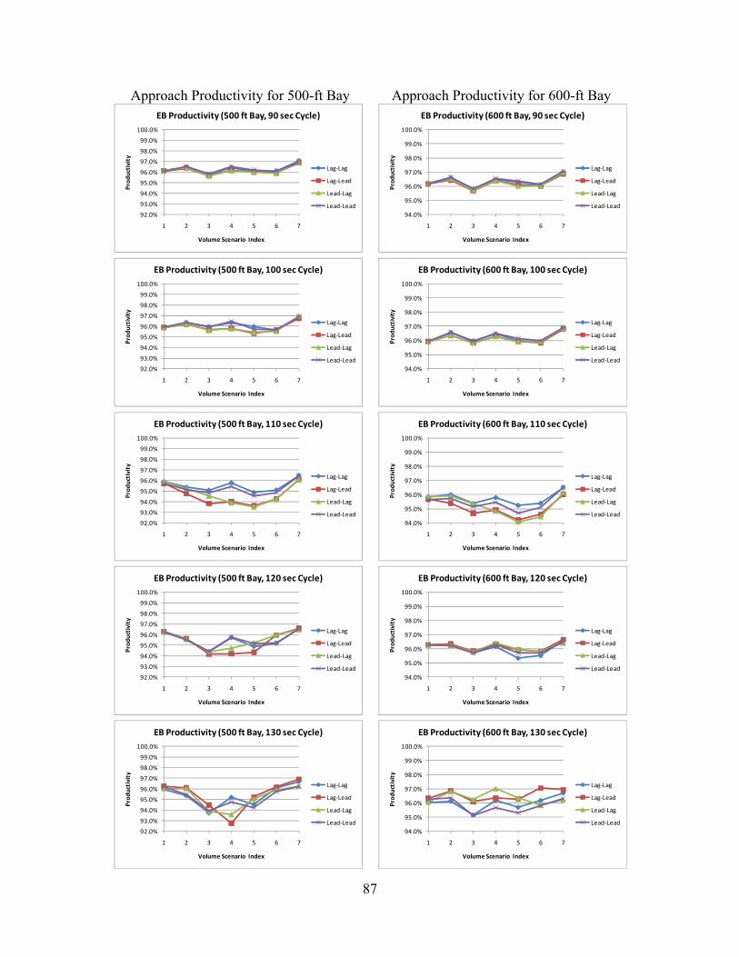
87
Approach Productivity for 500-ft Bay Approach Productivity for 600-ft Bay
92.0%
93.0%
94.0%
95.0%
96.0%
97.0%
98.0%
99.0%
100.0%
1 2 3 4 5 6 7
Prod
uctivity
Volume Scenario Index
EB Productivity (500 ft Bay, 90 sec Cycle)
Lag‐Lag
Lag‐Lead
Lead‐Lag
Lead‐Lead
92.0%
93.0%
94.0%
95.0%
96.0%
97.0%
98.0%
99.0%
100.0%
1 2 3 4 5 6 7
Prod
uctivity
Volume Scenario Index
EB Productivity (500 ft Bay, 100 sec Cycle)
Lag‐Lag
Lag‐Lead
Lead‐Lag
Lead‐Lead
92.0%
93.0%
94.0%
95.0%
96.0%
97.0%
98.0%
99.0%
100.0%
1 2 3 4 5 6 7
Prod
uctivity
Volume Scenario Index
EB Productivity (500 ft Bay, 110 sec Cycle)
Lag‐Lag
Lag‐Lead
Lead‐Lag
Lead‐Lead
92.0%
93.0%
94.0%
95.0%
96.0%
97.0%
98.0%
99.0%
100.0%
1 2 3 4 5 6 7
Prod
uctivity
Volume Scenario Index
EB Productivity (500 ft Bay, 120 sec Cycle)
Lag‐Lag
Lag‐Lead
Lead‐Lag
Lead‐Lead
92.0%
93.0%
94.0%
95.0%
96.0%
97.0%
98.0%
99.0%
100.0%
1 2 3 4 5 6 7
Prod
uctivity
Volume Scenario Index
EB Productivity (500 ft Bay, 130 sec Cycle)
Lag‐Lag
Lag‐Lead
Lead‐Lag
Lead‐Lead
94.0%
95.0%
96.0%
97.0%
98.0%
99.0%
100.0%
1 2 3 4 5 6 7
Prod
uctivity
Volume Scenario Index
EB Productivity (600 ft Bay, 90 sec Cycle)
Lag‐Lag
Lag‐Lead
Lead‐Lag
Lead‐Lead
94.0%
95.0%
96.0%
97.0%
98.0%
99.0%
100.0%
1 2 3 4 5 6 7
Prod
uctivity
Volume Scenario Index
EB Productivity (600 ft Bay, 100 sec Cycle)
Lag‐Lag
Lag‐Lead
Lead‐Lag
Lead‐Lead
94.0%
95.0%
96.0%
97.0%
98.0%
99.0%
100.0%
1 2 3 4 5 6 7
Prod
uctivity
Volume Scenario Index
EB Productivity (600 ft Bay, 110 sec Cycle)
Lag‐Lag
Lag‐Lead
Lead‐Lag
Lead‐Lead
94.0%
95.0%
96.0%
97.0%
98.0%
99.0%
100.0%
1 2 3 4 5 6 7
Prod
uctivity
Volume Scenario Index
EB Productivity (600 ft Bay, 120 sec Cycle)
Lag‐Lag
Lag‐Lead
Lead‐Lag
Lead‐Lead
94.0%
95.0%
96.0%
97.0%
98.0%
99.0%
100.0%
1 2 3 4 5 6 7
Prod
uctivity
Volume Scenario Index
EB Productivity (600 ft Bay, 130 sec Cycle)
Lag‐Lag
Lag‐Lead
Lead‐Lag
Lead‐Lead
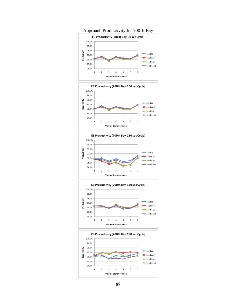
88
Approach Productivity for 700-ft Bay
94.0%
95.0%
96.0%
97.0%
98.0%
99.0%
100.0%
1 2 3 4 5 6 7
Prod
uctivity
Volume Scenario Index
EB Productivity (700 ft Bay, 90 sec Cycle)
Lag‐Lag
Lag‐Lead
Lead‐Lag
Lead‐Lead
94.0%
95.0%
96.0%
97.0%
98.0%
99.0%
100.0%
1 2 3 4 5 6 7
Prod
uctivity
Volume Scenario Index
EB Productivity (700 ft Bay, 100 sec Cycle)
Lag‐Lag
Lag‐Lead
Lead‐Lag
Lead‐Lead
94.0%
95.0%
96.0%
97.0%
98.0%
99.0%
100.0%
1 2 3 4 5 6 7
Prod
uctivity
Volume Scenario Index
EB Productivity (700 ft Bay, 110 sec Cycle)
Lag‐Lag
Lag‐Lead
Lead‐Lag
Lead‐Lead
94.0%
95.0%
96.0%
97.0%
98.0%
99.0%
100.0%
1 2 3 4 5 6 7
Prod
uctivity
Volume Scenario Index
EB Productivity (700 ft Bay, 120 sec Cycle)
Lag‐Lag
Lag‐Lead
Lead‐Lag
Lead‐Lead
94.0%
95.0%
96.0%
97.0%
98.0%
99.0%
100.0%
1 2 3 4 5 6 7
Prod
uctivity
Volume Scenario Index
EB Productivity (700 ft Bay, 130 sec Cycle)
Lag‐Lag
Lag‐Lead
Lead‐Lag
Lead‐Lead

89
APPENDIX D: SIMULATION RESULTS FOR THE FULLY-ACTUATED CONTROL SCENARIO


91
Approach Productivity for 100-ft Bay Approach Productivity for 200-ft Bay
40.0%
50.0%
60.0%
70.0%
80.0%
90.0%
100.0%
1 2 3 4 5 6 7
Prod
uctivity
Volume Scenario Index
EB Productivity (100 ft Bay, 90 sec Cycle)
Lag‐Lag
Lag‐Lead
Lead‐Lag
Lead‐Lead
40.0%
50.0%
60.0%
70.0%
80.0%
90.0%
100.0%
1 2 3 4 5 6 7
Prod
uctivity
Volume Scenario Index
EB Productivity (100 ft Bay, 100 sec Cycle)
Lag‐Lag
Lag‐Lead
Lead‐Lag
Lead‐Lead
40.0%
50.0%
60.0%
70.0%
80.0%
90.0%
100.0%
1 2 3 4 5 6 7
Prod
uctivity
Volume Scenario Index
EB Productivity (100 ft Bay, 110 sec Cycle)
Lag‐Lag
Lag‐Lead
Lead‐Lag
Lead‐Lead
40.0%
50.0%
60.0%
70.0%
80.0%
90.0%
100.0%
1 2 3 4 5 6 7
Prod
uctivity
Volume Scenario Index
EB Productivity (100 ft Bay, 120 sec Cycle)
Lag‐Lag
Lag‐Lead
Lead‐Lag
Lead‐Lead
40.0%
50.0%
60.0%
70.0%
80.0%
90.0%
100.0%
1 2 3 4 5 6 7
Prod
uctivity
Volume Scenario Index
EB Productivity (100 ft Bay, 130 sec Cycle)
Lag‐Lag
Lag‐Lead
Lead‐Lag
Lead‐Lead
60.0%
65.0%
70.0%
75.0%
80.0%
85.0%
90.0%
95.0%
100.0%
1 2 3 4 5 6 7
Prod
uctivity
Volume Scenario Index
EB Productivity (200 ft Bay, 90 sec Cycle)
Lag‐Lag
Lag‐Lead
Lead‐Lag
Lead‐Lead
60.0%
65.0%
70.0%
75.0%
80.0%
85.0%
90.0%
95.0%
100.0%
1 2 3 4 5 6 7
Prod
uctivity
Volume Scenario Index
EB Productivity (200 ft Bay, 100 sec Cycle)
Lag‐Lag
Lag‐Lead
Lead‐Lag
Lead‐Lead
60.0%
65.0%
70.0%
75.0%
80.0%
85.0%
90.0%
95.0%
100.0%
1 2 3 4 5 6 7
Prod
uctivity
Volume Scenario Index
EB Productivity (200 ft Bay, 110 sec Cycle)
Lag‐Lag
Lag‐Lead
Lead‐Lag
Lead‐Lead
60.0%
65.0%
70.0%
75.0%
80.0%
85.0%
90.0%
95.0%
100.0%
1 2 3 4 5 6 7
Prod
uctivity
Volume Scenario Index
EB Productivity (200 ft Bay, 120 sec Cycle)
Lag‐Lag
Lag‐Lead
Lead‐Lag
Lead‐Lead
60.0%
65.0%
70.0%
75.0%
80.0%
85.0%
90.0%
95.0%
100.0%
1 2 3 4 5 6 7
Prod
uctivity
Volume Scenario Index
EB Productivity (200 ft Bay, 130 sec Cycle)
Lag‐Lag
Lag‐Lead
Lead‐Lag
Lead‐Lead

92
Approach Productivity for 300-ft Bay Approach Productivity for 400-ft Bay
70.0%
75.0%
80.0%
85.0%
90.0%
95.0%
100.0%
1 2 3 4 5 6 7
Prod
uctivity
Volume Scenario Index
EB Productivity (300 ft Bay, 90 sec Cycle)
Lag‐Lag
Lag‐Lead
Lead‐Lag
Lead‐Lead
70.0%
75.0%
80.0%
85.0%
90.0%
95.0%
100.0%
1 2 3 4 5 6 7
Prod
uctivity
Volume Scenario Index
EB Productivity (300 ft Bay, 100 sec Cycle)
Lag‐Lag
Lag‐Lead
Lead‐Lag
Lead‐Lead
70.0%
75.0%
80.0%
85.0%
90.0%
95.0%
100.0%
1 2 3 4 5 6 7
Prod
uctivity
Volume Scenario Index
EB Productivity (300 ft Bay, 110 sec Cycle)
Lag‐Lag
Lag‐Lead
Lead‐Lag
Lead‐Lead
70.0%
75.0%
80.0%
85.0%
90.0%
95.0%
100.0%
1 2 3 4 5 6 7
Prod
uctivity
Volume Scenario Index
EB Productivity (300 ft Bay, 120 sec Cycle)
Lag‐Lag
Lag‐Lead
Lead‐Lag
Lead‐Lead
70.0%
75.0%
80.0%
85.0%
90.0%
95.0%
100.0%
1 2 3 4 5 6 7
Prod
uctivity
Volume Scenario Index
EB Productivity (300 ft Bay, 130 sec Cycle)
Lag‐Lag
Lag‐Lead
Lead‐Lag
Lead‐Lead
75.0%
80.0%
85.0%
90.0%
95.0%
100.0%
1 2 3 4 5 6 7
Prod
uctivity
Volume Scenario Index
EB Productivity (400 ft Bay, 90 sec Cycle)
Lag‐Lag
Lag‐Lead
Lead‐Lag
Lead‐Lead
75.0%
80.0%
85.0%
90.0%
95.0%
100.0%
1 2 3 4 5 6 7
Prod
uctivity
Volume Scenario Index
EB Productivity (400 ft Bay, 100 sec Cycle)
Lag‐Lag
Lag‐Lead
Lead‐Lag
Lead‐Lead
75.0%
80.0%
85.0%
90.0%
95.0%
100.0%
1 2 3 4 5 6 7
Prod
uctivity
Volume Scenario Index
EB Productivity (400 ft Bay, 110 sec Cycle)
Lag‐Lag
Lag‐Lead
Lead‐Lag
Lead‐Lead
75.0%
80.0%
85.0%
90.0%
95.0%
100.0%
1 2 3 4 5 6 7
Prod
uctivity
Volume Scenario Index
EB Productivity (400 ft Bay, 120 sec Cycle)
Lag‐Lag
Lag‐Lead
Lead‐Lag
Lead‐Lead
75.0%
80.0%
85.0%
90.0%
95.0%
100.0%
1 2 3 4 5 6 7
Prod
uctivity
Volume Scenario Index
EB Productivity (400 ft Bay, 130 sec Cycle)
Lag‐Lag
Lag‐Lead
Lead‐Lag
Lead‐Lead

93
Approach Productivity for 500-ft Bay Approach Productivity for 600-ft Bay
85.0%
87.0%
89.0%
91.0%
93.0%
95.0%
97.0%
99.0%
1 2 3 4 5 6 7
Prod
uctivity
Volume Scenario Index
EB Productivity (500 ft Bay, 90 sec Cycle)
Lag‐Lag
Lag‐Lead
Lead‐Lag
Lead‐Lead
85.0%
87.0%
89.0%
91.0%
93.0%
95.0%
97.0%
99.0%
1 2 3 4 5 6 7
Prod
uctivity
Volume Scenario Index
EB Productivity (500 ft Bay, 100 sec Cycle)
Lag‐Lag
Lag‐Lead
Lead‐Lag
Lead‐Lead
85.0%
87.0%
89.0%
91.0%
93.0%
95.0%
97.0%
99.0%
1 2 3 4 5 6 7
Prod
uctivity
Volume Scenario Index
EB Productivity (500 ft Bay, 110 sec Cycle)
Lag‐Lag
Lag‐Lead
Lead‐Lag
Lead‐Lead
85.0%
87.0%
89.0%
91.0%
93.0%
95.0%
97.0%
99.0%
1 2 3 4 5 6 7
Prod
uctivity
Volume Scenario Index
EB Productivity (500 ft Bay, 120 sec Cycle)
Lag‐Lag
Lag‐Lead
Lead‐Lag
Lead‐Lead
85.0%
87.0%
89.0%
91.0%
93.0%
95.0%
97.0%
99.0%
1 2 3 4 5 6 7
Prod
uctivity
Volume Scenario Index
EB Productivity (500 ft Bay, 130 sec Cycle)
Lag‐Lag
Lag‐Lead
Lead‐Lag
Lead‐Lead
85.0%
87.0%
89.0%
91.0%
93.0%
95.0%
97.0%
99.0%
1 2 3 4 5 6 7
Prod
uctivity
Volume Scenario Index
EB Productivity (600 ft Bay, 90 sec Cycle)
Lag‐Lag
Lag‐Lead
Lead‐Lag
Lead‐Lead
85.0%
87.0%
89.0%
91.0%
93.0%
95.0%
97.0%
99.0%
1 2 3 4 5 6 7
Prod
uctivity
Volume Scenario Index
EB Productivity (600 ft Bay, 100 sec Cycle)
Lag‐Lag
Lag‐Lead
Lead‐Lag
Lead‐Lead
85.0%
87.0%
89.0%
91.0%
93.0%
95.0%
97.0%
99.0%
1 2 3 4 5 6 7
Prod
uctivity
Volume Scenario Index
EB Productivity (600 ft Bay, 110 sec Cycle)
Lag‐Lag
Lag‐Lead
Lead‐Lag
Lead‐Lead
85.0%
87.0%
89.0%
91.0%
93.0%
95.0%
97.0%
99.0%
1 2 3 4 5 6 7
Prod
uctivity
Volume Scenario Index
EB Productivity (600 ft Bay, 120 sec Cycle)
Lag‐Lag
Lag‐Lead
Lead‐Lag
Lead‐Lead
85.0%
87.0%
89.0%
91.0%
93.0%
95.0%
97.0%
99.0%
1 2 3 4 5 6 7
Prod
uctivity
Volume Scenario Index
EB Productivity (600 ft Bay, 130 sec Cycle)
Lag‐Lag
Lag‐Lead
Lead‐Lag
Lead‐Lead

94
Approach Productivity for 700-ft Bay
90.0%91.0%92.0%93.0%94.0%95.0%96.0%97.0%98.0%99.0%
100.0%
1 2 3 4 5 6 7
Prod
uctivity
Volume Scenario Index
EB Productivity (700 ft Bay, 90 sec Cycle)
Lag‐Lag
Lag‐Lead
Lead‐Lag
Lead‐Lead
90.0%91.0%92.0%93.0%94.0%95.0%96.0%97.0%98.0%99.0%
100.0%
1 2 3 4 5 6 7
Prod
uctivity
Volume Scenario Index
EB Productivity (700 ft Bay, 100 sec Cycle)
Lag‐Lag
Lag‐Lead
Lead‐Lag
Lead‐Lead
90.0%91.0%92.0%93.0%94.0%95.0%96.0%97.0%98.0%99.0%
100.0%
1 2 3 4 5 6 7
Prod
uctivity
Volume Scenario Index
EB Productivity (700 ft Bay, 110 sec Cycle)
Lag‐Lag
Lag‐Lead
Lead‐Lag
Lead‐Lead
90.0%91.0%92.0%93.0%94.0%95.0%96.0%97.0%98.0%99.0%
100.0%
1 2 3 4 5 6 7
Prod
uctivity
Volume Scenario Index
EB Productivity (700 ft Bay, 120 sec Cycle)
Lag‐Lag
Lag‐Lead
Lead‐Lag
Lead‐Lead
90.0%91.0%92.0%93.0%94.0%95.0%96.0%97.0%98.0%99.0%
100.0%
1 2 3 4 5 6 7
Prod
uctivity
Volume Scenario Index
EB Productivity (700 ft Bay, 130 sec Cycle)
Lag‐Lag
Lag‐Lead
Lead‐Lag
Lead‐Lead

95
APPENDIX E: SIMULATION RESULTS FOR DUAL LEFT-TURN BAY WITH FIXED-TIME CONTROL AND PREVIOUS TIMINGS

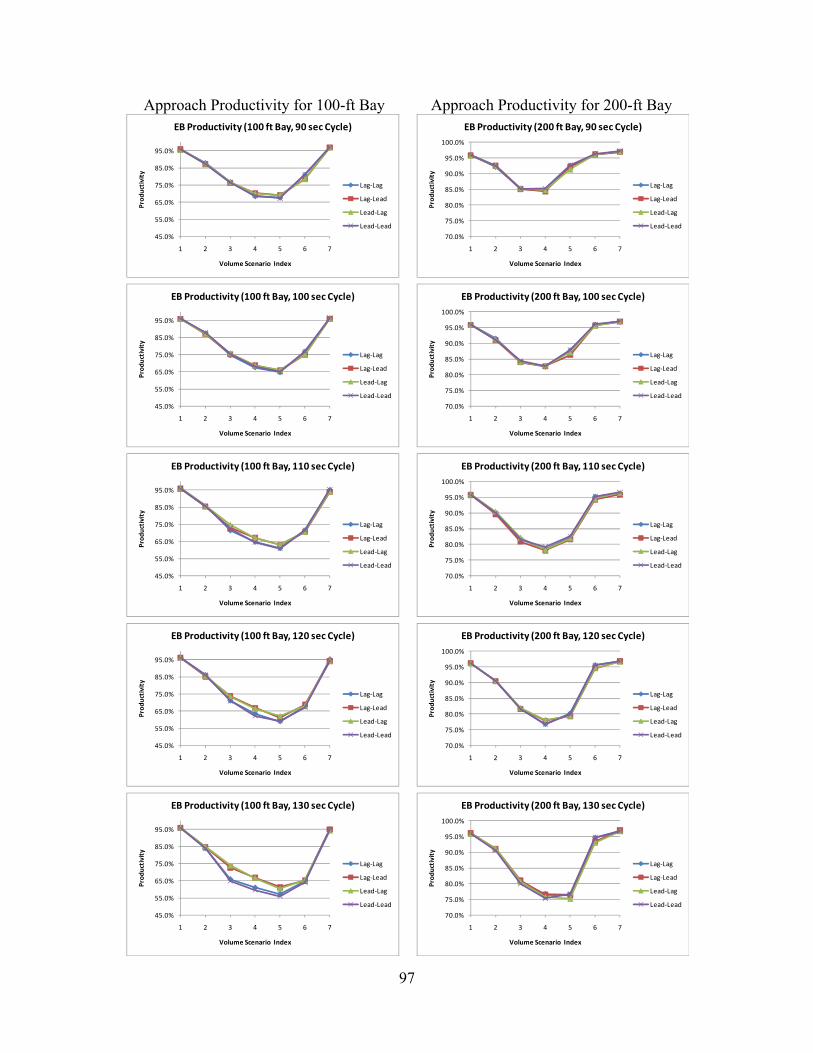
97
Approach Productivity for 100-ft Bay Approach Productivity for 200-ft Bay
45.0%
55.0%
65.0%
75.0%
85.0%
95.0%
1 2 3 4 5 6 7
Prod
uctivity
Volume Scenario Index
EB Productivity (100 ft Bay, 90 sec Cycle)
Lag‐Lag
Lag‐Lead
Lead‐Lag
Lead‐Lead
45.0%
55.0%
65.0%
75.0%
85.0%
95.0%
1 2 3 4 5 6 7
Prod
uctivity
Volume Scenario Index
EB Productivity (100 ft Bay, 100 sec Cycle)
Lag‐Lag
Lag‐Lead
Lead‐Lag
Lead‐Lead
45.0%
55.0%
65.0%
75.0%
85.0%
95.0%
1 2 3 4 5 6 7
Prod
uctivity
Volume Scenario Index
EB Productivity (100 ft Bay, 110 sec Cycle)
Lag‐Lag
Lag‐Lead
Lead‐Lag
Lead‐Lead
45.0%
55.0%
65.0%
75.0%
85.0%
95.0%
1 2 3 4 5 6 7
Prod
uctivity
Volume Scenario Index
EB Productivity (100 ft Bay, 120 sec Cycle)
Lag‐Lag
Lag‐Lead
Lead‐Lag
Lead‐Lead
45.0%
55.0%
65.0%
75.0%
85.0%
95.0%
1 2 3 4 5 6 7
Prod
uctivity
Volume Scenario Index
EB Productivity (100 ft Bay, 130 sec Cycle)
Lag‐Lag
Lag‐Lead
Lead‐Lag
Lead‐Lead
70.0%
75.0%
80.0%
85.0%
90.0%
95.0%
100.0%
1 2 3 4 5 6 7
Prod
uctivity
Volume Scenario Index
EB Productivity (200 ft Bay, 90 sec Cycle)
Lag‐Lag
Lag‐Lead
Lead‐Lag
Lead‐Lead
70.0%
75.0%
80.0%
85.0%
90.0%
95.0%
100.0%
1 2 3 4 5 6 7
Prod
uctivity
Volume Scenario Index
EB Productivity (200 ft Bay, 100 sec Cycle)
Lag‐Lag
Lag‐Lead
Lead‐Lag
Lead‐Lead
70.0%
75.0%
80.0%
85.0%
90.0%
95.0%
100.0%
1 2 3 4 5 6 7
Prod
uctivity
Volume Scenario Index
EB Productivity (200 ft Bay, 110 sec Cycle)
Lag‐Lag
Lag‐Lead
Lead‐Lag
Lead‐Lead
70.0%
75.0%
80.0%
85.0%
90.0%
95.0%
100.0%
1 2 3 4 5 6 7
Prod
uctivity
Volume Scenario Index
EB Productivity (200 ft Bay, 120 sec Cycle)
Lag‐Lag
Lag‐Lead
Lead‐Lag
Lead‐Lead
70.0%
75.0%
80.0%
85.0%
90.0%
95.0%
100.0%
1 2 3 4 5 6 7
Prod
uctivity
Volume Scenario Index
EB Productivity (200 ft Bay, 130 sec Cycle)
Lag‐Lag
Lag‐Lead
Lead‐Lag
Lead‐Lead

98
Approach Productivity for 300-ft Bay Approach Productivity for 400-ft Bay
75.0%
80.0%
85.0%
90.0%
95.0%
100.0%
1 2 3 4 5 6 7
Prod
uctivity
Volume Scenario Index
EB Productivity (300 ft Bay, 90 sec Cycle)
Lag‐Lag
Lag‐Lead
Lead‐Lag
Lead‐Lead
75.0%
80.0%
85.0%
90.0%
95.0%
100.0%
1 2 3 4 5 6 7
Prod
uctivity
Volume Scenario Index
EB Productivity (300 ft Bay, 100 sec Cycle)
Lag‐Lag
Lag‐Lead
Lead‐Lag
Lead‐Lead
75.0%
80.0%
85.0%
90.0%
95.0%
100.0%
1 2 3 4 5 6 7
Prod
uctivity
Volume Scenario Index
EB Productivity (300 ft Bay, 110 sec Cycle)
Lag‐Lag
Lag‐Lead
Lead‐Lag
Lead‐Lead
75.0%
80.0%
85.0%
90.0%
95.0%
100.0%
1 2 3 4 5 6 7
Prod
uctivity
Volume Scenario Index
EB Productivity (300 ft Bay, 120 sec Cycle)
Lag‐Lag
Lag‐Lead
Lead‐Lag
Lead‐Lead
75.0%
80.0%
85.0%
90.0%
95.0%
100.0%
1 2 3 4 5 6 7
Prod
uctivity
Volume Scenario Index
EB Productivity (300 ft Bay, 130 sec Cycle)
Lag‐Lag
Lag‐Lead
Lead‐Lag
Lead‐Lead
88.0%
90.0%
92.0%
94.0%
96.0%
98.0%
100.0%
1 2 3 4 5 6 7
Prod
uctivity
Volume Scenario Index
EB Productivity (400 ft Bay, 90 sec Cycle)
Lag‐Lag
Lag‐Lead
Lead‐Lag
Lead‐Lead
88.0%
90.0%
92.0%
94.0%
96.0%
98.0%
100.0%
1 2 3 4 5 6 7
Prod
uctivity
Volume Scenario Index
EB Productivity (400 ft Bay, 100 sec Cycle)
Lag‐Lag
Lag‐Lead
Lead‐Lag
Lead‐Lead
88.0%
90.0%
92.0%
94.0%
96.0%
98.0%
100.0%
1 2 3 4 5 6 7
Prod
uctivity
Volume Scenario Index
EB Productivity (400 ft Bay, 110 sec Cycle)
Lag‐Lag
Lag‐Lead
Lead‐Lag
Lead‐Lead
88.0%
90.0%
92.0%
94.0%
96.0%
98.0%
100.0%
1 2 3 4 5 6 7
Prod
uctivity
Volume Scenario Index
EB Productivity (400 ft Bay, 120 sec Cycle)
Lag‐Lag
Lag‐Lead
Lead‐Lag
Lead‐Lead
88.0%
90.0%
92.0%
94.0%
96.0%
98.0%
100.0%
1 2 3 4 5 6 7
Prod
uctivity
Volume Scenario Index
EB Productivity (400 ft Bay, 130 sec Cycle)
Lag‐Lag
Lag‐Lead
Lead‐Lag
Lead‐Lead

99
Approach Productivity for 500-ft Bay Approach Productivity for 600-ft Bay
93.0%
94.0%
95.0%
96.0%
97.0%
98.0%
99.0%
100.0%
1 2 3 4 5 6 7
Prod
uctivity
Volume Scenario Index
EB Productivity (500 ft Bay, 90 sec Cycle)
Lag‐Lag
Lag‐Lead
Lead‐Lag
Lead‐Lead
93.0%
94.0%
95.0%
96.0%
97.0%
98.0%
99.0%
100.0%
1 2 3 4 5 6 7
Prod
uctivity
Volume Scenario Index
EB Productivity (500 ft Bay, 100 sec Cycle)
Lag‐Lag
Lag‐Lead
Lead‐Lag
Lead‐Lead
93.0%
94.0%
95.0%
96.0%
97.0%
98.0%
99.0%
100.0%
1 2 3 4 5 6 7
Prod
uctivity
Volume Scenario Index
EB Productivity (500 ft Bay, 110 sec Cycle)
Lag‐Lag
Lag‐Lead
Lead‐Lag
Lead‐Lead
93.0%
94.0%
95.0%
96.0%
97.0%
98.0%
99.0%
100.0%
1 2 3 4 5 6 7
Prod
uctivity
Volume Scenario Index
EB Productivity (500 ft Bay, 120 sec Cycle)
Lag‐Lag
Lag‐Lead
Lead‐Lag
Lead‐Lead
93.0%
94.0%
95.0%
96.0%
97.0%
98.0%
99.0%
100.0%
1 2 3 4 5 6 7
Prod
uctivity
Volume Scenario Index
EB Productivity (500 ft Bay, 130 sec Cycle)
Lag‐Lag
Lag‐Lead
Lead‐Lag
Lead‐Lead
93.0%
94.0%
95.0%
96.0%
97.0%
98.0%
99.0%
100.0%
1 2 3 4 5 6 7
Prod
uctivity
Volume Scenario Index
EB Productivity (600 ft Bay, 90 sec Cycle)
Lag‐Lag
Lag‐Lead
Lead‐Lag
Lead‐Lead
93.0%
94.0%
95.0%
96.0%
97.0%
98.0%
99.0%
100.0%
1 2 3 4 5 6 7
Prod
uctivity
Volume Scenario Index
EB Productivity (600 ft Bay, 100 sec Cycle)
Lag‐Lag
Lag‐Lead
Lead‐Lag
Lead‐Lead
93.0%
94.0%
95.0%
96.0%
97.0%
98.0%
99.0%
100.0%
1 2 3 4 5 6 7
Prod
uctivity
Volume Scenario Index
EB Productivity (600 ft Bay, 110 sec Cycle)
Lag‐Lag
Lag‐Lead
Lead‐Lag
Lead‐Lead
93.0%
94.0%
95.0%
96.0%
97.0%
98.0%
99.0%
100.0%
1 2 3 4 5 6 7
Prod
uctivity
Volume Scenario Index
EB Productivity (600 ft Bay, 120 sec Cycle)
Lag‐Lag
Lag‐Lead
Lead‐Lag
Lead‐Lead
93.0%
94.0%
95.0%
96.0%
97.0%
98.0%
99.0%
100.0%
1 2 3 4 5 6 7
Prod
uctivity
Volume Scenario Index
EB Productivity (600 ft Bay, 130 sec Cycle)
Lag‐Lag
Lag‐Lead
Lead‐Lag
Lead‐Lead
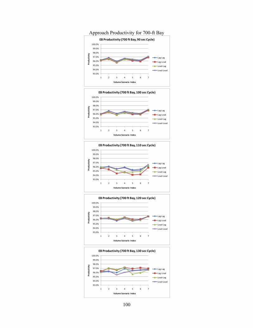
100
Approach Productivity for 700-ft Bay
93.0%
94.0%
95.0%
96.0%
97.0%
98.0%
99.0%
100.0%
1 2 3 4 5 6 7
Prod
uctivity
Volume Scenario Index
EB Productivity (700 ft Bay, 90 sec Cycle)
Lag‐Lag
Lag‐Lead
Lead‐Lag
Lead‐Lead
93.0%
94.0%
95.0%
96.0%
97.0%
98.0%
99.0%
100.0%
1 2 3 4 5 6 7
Prod
uctivity
Volume Scenario Index
EB Productivity (700 ft Bay, 100 sec Cycle)
Lag‐Lag
Lag‐Lead
Lead‐Lag
Lead‐Lead
93.0%
94.0%
95.0%
96.0%
97.0%
98.0%
99.0%
100.0%
1 2 3 4 5 6 7
Prod
uctivity
Volume Scenario Index
EB Productivity (700 ft Bay, 110 sec Cycle)
Lag‐Lag
Lag‐Lead
Lead‐Lag
Lead‐Lead
93.0%
94.0%
95.0%
96.0%
97.0%
98.0%
99.0%
100.0%
1 2 3 4 5 6 7
Prod
uctivity
Volume Scenario Index
EB Productivity (700 ft Bay, 120 sec Cycle)
Lag‐Lag
Lag‐Lead
Lead‐Lag
Lead‐Lead
93.0%
94.0%
95.0%
96.0%
97.0%
98.0%
99.0%
100.0%
1 2 3 4 5 6 7
Prod
uctivity
Volume Scenario Index
EB Productivity (700 ft Bay, 130 sec Cycle)
Lag‐Lag
Lag‐Lead
Lead‐Lag
Lead‐Lead

101
APPENDIX F: PERCENT DEMAND SERVED FOR SELECTED CASES OF SINGLE LEFT-TURN LANE WITH FIXED-TIME TRAFFIC SIGNAL


103
Approach Productivity for 100-ft Bay and 100-second Cycle
Approach Productivity for 300-ft Bay and 100-second Cycle
Approach Productivity for 500-ft Bay and 100-second Cycle
45.0%
55.0%
65.0%
75.0%
85.0%
95.0%
1 2 3 4 5 6 7
Prod
uctivity
Volume Scenario Index
EB Percent Demand Served (100 ft Bay, 100 sec Cycle)
Lag‐Lag
Lag‐Lead
Lead‐Lag
Lead‐Lead
75.0%
80.0%
85.0%
90.0%
95.0%
100.0%
1 2 3 4 5 6 7
Prod
uctivity
Volume Scenario Index
EB Percent Demand Served (300 ft Bay, 100 sec Cycle)
Lag‐Lag
Lag‐Lead
Lead‐Lag
Lead‐Lead
92.0%
93.0%
94.0%
95.0%
96.0%
97.0%
98.0%
99.0%
100.0%
1 2 3 4 5 6 7
Prod
uctivity
Volume Scenario Index
EB Percent Demand Served (500 ft Bay, 100 sec Cycle)
Lag‐Lag
Lag‐Lead
Lead‐Lag
Lead‐Lead


105
APPENDIX G: SIMULATION RESULTS FOR DUAL LEFT-TURN BAY WITH FIXED-TIME CONTROL AND RETIMED SIGNAL


107
Approach Productivity for 100-ft Bay Approach Productivity for 200-ft Bay
45.0%
55.0%
65.0%
75.0%
85.0%
95.0%
1 2 3 4 5 6 7
Prod
uctivity
Volume Scenario Index
EB Percent Demand Served (100 ft Bay, 90 sec Cycle)
Lag‐Lag
Lag‐Lead
Lead‐Lag
Lead‐Lead
45.0%
55.0%
65.0%
75.0%
85.0%
95.0%
1 2 3 4 5 6 7
Prod
uctivity
Volume Scenario Index
EB Percent Demand Served (100 ft Bay, 100 sec Cycle)
Lag‐Lag
Lag‐Lead
Lead‐Lag
Lead‐Lead
45.0%
55.0%
65.0%
75.0%
85.0%
95.0%
1 2 3 4 5 6 7
Prod
uctivity
Volume Scenario Index
EB Percent Demand Served (100 ft Bay, 110 sec Cycle)
Lag‐Lag
Lag‐Lead
Lead‐Lag
Lead‐Lead
45.0%
55.0%
65.0%
75.0%
85.0%
95.0%
1 2 3 4 5 6 7
Prod
uctivity
Volume Scenario Index
EB Percent Demand Served (100 ft Bay, 120 sec Cycle)
Lag‐Lag
Lag‐Lead
Lead‐Lag
Lead‐Lead
45.0%
55.0%
65.0%
75.0%
85.0%
95.0%
1 2 3 4 5 6 7
Prod
uctivity
Volume Scenario Index
EB Percent Demand Served (100 ft Bay, 130 sec Cycle)
Lag‐Lag
Lag‐Lead
Lead‐Lag
Lead‐Lead
70.0%
75.0%
80.0%
85.0%
90.0%
95.0%
100.0%
1 2 3 4 5 6 7
Prod
uctivity
Volume Scenario Index
EB Percent Demand Served (200 ft Bay, 90 sec Cycle)
Lag‐Lag
Lag‐Lead
Lead‐Lag
Lead‐Lead
70.0%
75.0%
80.0%
85.0%
90.0%
95.0%
100.0%
1 2 3 4 5 6 7
Prod
uctivity
Volume Scenario Index
EB Percent Demand Served (200 ft Bay, 100 sec Cycle)
Lag‐Lag
Lag‐Lead
Lead‐Lag
Lead‐Lead
70.0%
75.0%
80.0%
85.0%
90.0%
95.0%
100.0%
1 2 3 4 5 6 7
Prod
uctivity
Volume Scenario Index
EB Percent Demand Served (200 ft Bay, 110 sec Cycle)
Lag‐Lag
Lag‐Lead
Lead‐Lag
Lead‐Lead
70.0%
75.0%
80.0%
85.0%
90.0%
95.0%
100.0%
1 2 3 4 5 6 7
Prod
uctivity
Volume Scenario Index
EB Percent Demand Served (200 ft Bay, 120 sec Cycle)
Lag‐Lag
Lag‐Lead
Lead‐Lag
Lead‐Lead
70.0%
75.0%
80.0%
85.0%
90.0%
95.0%
100.0%
1 2 3 4 5 6 7
Prod
uctivity
Volume Scenario Index
EB Percent Demand Served (200 ft Bay, 130 sec Cycle)
Lag‐Lag
Lag‐Lead
Lead‐Lag
Lead‐Lead

108
Approach Productivity for 300-ft Bay Approach Productivity for 400-ft Bay
75.0%
80.0%
85.0%
90.0%
95.0%
100.0%
1 2 3 4 5 6 7
Prod
uctivity
Volume Scenario Index
EB Percent Demand Served (300 ft Bay, 90 sec Cycle)
Lag‐Lag
Lag‐Lead
Lead‐Lag
Lead‐Lead
75.0%
80.0%
85.0%
90.0%
95.0%
100.0%
1 2 3 4 5 6 7
Prod
uctivity
Volume Scenario Index
EB Percent Demand Served (300 ft Bay, 100 sec Cycle)
Lag‐Lag
Lag‐Lead
Lead‐Lag
Lead‐Lead
75.0%
80.0%
85.0%
90.0%
95.0%
100.0%
1 2 3 4 5 6 7
Prod
uctivity
Volume Scenario Index
EB Percent Demand Served (300 ft Bay, 110 sec Cycle)
Lag‐Lag
Lag‐Lead
Lead‐Lag
Lead‐Lead
75.0%
80.0%
85.0%
90.0%
95.0%
100.0%
1 2 3 4 5 6 7
Prod
uctivity
Volume Scenario Index
EB Percent Demand Served (300 ft Bay, 120 sec Cycle)
Lag‐Lag
Lag‐Lead
Lead‐Lag
Lead‐Lead
75.0%
80.0%
85.0%
90.0%
95.0%
100.0%
1 2 3 4 5 6 7
Prod
uctivity
Volume Scenario Index
EB Percent Demand Served (300 ft Bay, 130 sec Cycle)
Lag‐Lag
Lag‐Lead
Lead‐Lag
Lead‐Lead
84.0%
86.0%
88.0%
90.0%
92.0%
94.0%
96.0%
98.0%
100.0%
1 2 3 4 5 6 7
Prod
uctivity
Volume Scenario Index
EB Percent Demand Served (400 ft Bay, 90 sec Cycle)
Lag‐Lag
Lag‐Lead
Lead‐Lag
Lead‐Lead
84.0%
86.0%
88.0%
90.0%
92.0%
94.0%
96.0%
98.0%
100.0%
1 2 3 4 5 6 7
Prod
uctivity
Volume Scenario Index
EB Percent Demand Served (400 ft Bay, 100 sec Cycle)
Lag‐Lag
Lag‐Lead
Lead‐Lag
Lead‐Lead
84.0%
86.0%
88.0%
90.0%
92.0%
94.0%
96.0%
98.0%
100.0%
1 2 3 4 5 6 7
Prod
uctivity
Volume Scenario Index
EB Percent Demand Served (400 ft Bay, 110 sec Cycle)
Lag‐Lag
Lag‐Lead
Lead‐Lag
Lead‐Lead
84.0%
86.0%
88.0%
90.0%
92.0%
94.0%
96.0%
98.0%
100.0%
1 2 3 4 5 6 7
Prod
uctivity
Volume Scenario Index
EB Percent Demand Served (400 ft Bay, 120 sec Cycle)
Lag‐Lag
Lag‐Lead
Lead‐Lag
Lead‐Lead
84.0%
86.0%
88.0%
90.0%
92.0%
94.0%
96.0%
98.0%
100.0%
1 2 3 4 5 6 7
Prod
uctivity
Volume Scenario Index
EB Percent Demand Served (400 ft Bay, 130 sec Cycle)
Lag‐Lag
Lag‐Lead
Lead‐Lag
Lead‐Lead
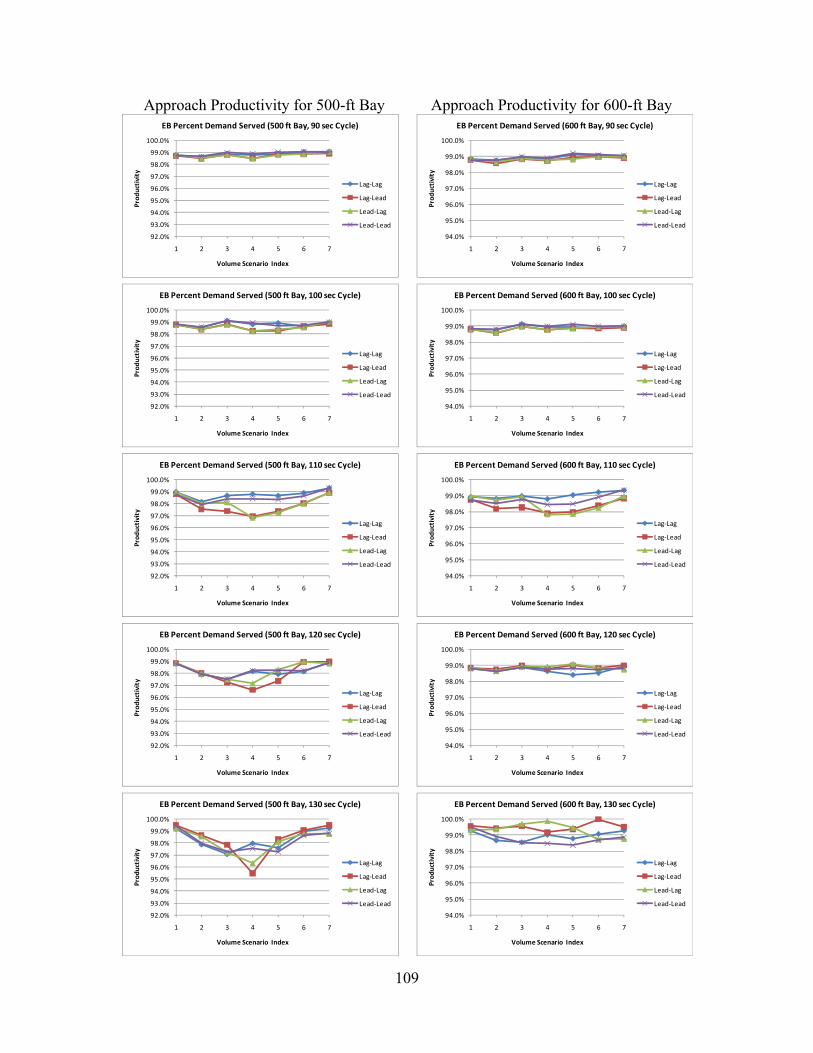
109
Approach Productivity for 500-ft Bay Approach Productivity for 600-ft Bay
92.0%
93.0%
94.0%
95.0%
96.0%
97.0%
98.0%
99.0%
100.0%
1 2 3 4 5 6 7
Prod
uctivity
Volume Scenario Index
EB Percent Demand Served (500 ft Bay, 90 sec Cycle)
Lag‐Lag
Lag‐Lead
Lead‐Lag
Lead‐Lead
92.0%
93.0%
94.0%
95.0%
96.0%
97.0%
98.0%
99.0%
100.0%
1 2 3 4 5 6 7
Prod
uctivity
Volume Scenario Index
EB Percent Demand Served (500 ft Bay, 100 sec Cycle)
Lag‐Lag
Lag‐Lead
Lead‐Lag
Lead‐Lead
92.0%
93.0%
94.0%
95.0%
96.0%
97.0%
98.0%
99.0%
100.0%
1 2 3 4 5 6 7
Prod
uctivity
Volume Scenario Index
EB Percent Demand Served (500 ft Bay, 110 sec Cycle)
Lag‐Lag
Lag‐Lead
Lead‐Lag
Lead‐Lead
92.0%
93.0%
94.0%
95.0%
96.0%
97.0%
98.0%
99.0%
100.0%
1 2 3 4 5 6 7
Prod
uctivity
Volume Scenario Index
EB Percent Demand Served (500 ft Bay, 120 sec Cycle)
Lag‐Lag
Lag‐Lead
Lead‐Lag
Lead‐Lead
92.0%
93.0%
94.0%
95.0%
96.0%
97.0%
98.0%
99.0%
100.0%
1 2 3 4 5 6 7
Prod
uctivity
Volume Scenario Index
EB Percent Demand Served (500 ft Bay, 130 sec Cycle)
Lag‐Lag
Lag‐Lead
Lead‐Lag
Lead‐Lead
94.0%
95.0%
96.0%
97.0%
98.0%
99.0%
100.0%
1 2 3 4 5 6 7
Prod
uctivity
Volume Scenario Index
EB Percent Demand Served (600 ft Bay, 90 sec Cycle)
Lag‐Lag
Lag‐Lead
Lead‐Lag
Lead‐Lead
94.0%
95.0%
96.0%
97.0%
98.0%
99.0%
100.0%
1 2 3 4 5 6 7
Prod
uctivity
Volume Scenario Index
EB Percent Demand Served (600 ft Bay, 100 sec Cycle)
Lag‐Lag
Lag‐Lead
Lead‐Lag
Lead‐Lead
94.0%
95.0%
96.0%
97.0%
98.0%
99.0%
100.0%
1 2 3 4 5 6 7
Prod
uctivity
Volume Scenario Index
EB Percent Demand Served (600 ft Bay, 110 sec Cycle)
Lag‐Lag
Lag‐Lead
Lead‐Lag
Lead‐Lead
94.0%
95.0%
96.0%
97.0%
98.0%
99.0%
100.0%
1 2 3 4 5 6 7
Prod
uctivity
Volume Scenario Index
EB Percent Demand Served (600 ft Bay, 120 sec Cycle)
Lag‐Lag
Lag‐Lead
Lead‐Lag
Lead‐Lead
94.0%
95.0%
96.0%
97.0%
98.0%
99.0%
100.0%
1 2 3 4 5 6 7
Prod
uctivity
Volume Scenario Index
EB Percent Demand Served (600 ft Bay, 130 sec Cycle)
Lag‐Lag
Lag‐Lead
Lead‐Lag
Lead‐Lead

110
Approach Productivity for 700-ft Bay
94.0%
95.0%
96.0%
97.0%
98.0%
99.0%
100.0%
1 2 3 4 5 6 7
Prod
uctivity
Volume Scenario Index
EB Percent Demand Served (700 ft Bay, 90 sec Cycle)
Lag‐Lag
Lag‐Lead
Lead‐Lag
Lead‐Lead
94.0%
95.0%
96.0%
97.0%
98.0%
99.0%
100.0%
1 2 3 4 5 6 7
Prod
uctivity
Volume Scenario Index
EB Percent Demand Served (700 ft Bay, 100 sec Cycle)
Lag‐Lag
Lag‐Lead
Lead‐Lag
Lead‐Lead
94.0%
95.0%
96.0%
97.0%
98.0%
99.0%
100.0%
1 2 3 4 5 6 7
Prod
uctivity
Volume Scenario Index
EB Percent Demand Served (700 ft Bay, 110 sec Cycle)
Lag‐Lag
Lag‐Lead
Lead‐Lag
Lead‐Lead
94.0%
95.0%
96.0%
97.0%
98.0%
99.0%
100.0%
1 2 3 4 5 6 7
Prod
uctivity
Volume Scenario Index
EB Percent Demand Served (700 ft Bay, 120 sec Cycle)
Lag‐Lag
Lag‐Lead
Lead‐Lag
Lead‐Lead
94.0%
95.0%
96.0%
97.0%
98.0%
99.0%
100.0%
1 2 3 4 5 6 7
Prod
uctivity
Volume Scenario Index
EB Percent Demand Served (700 ft Bay, 130 sec Cycle)
Lag‐Lag
Lag‐Lead
Lead‐Lag
Lead‐Lead