guideline for environmental characterization of semiconductor process equipment

Guideline for Environmental Characterization of Semiconductor Process Equipment

International SEMATECH Manufacturing Initiative Technology Transfer #06124825A-ENG

© 2006 International SEMATECH Manufacturing Initiative, Inc.

Advanced Materials Research Center, AMRC, International SEMATECH Manufacturing Initiative, and ISMI are servicemarks of SEMATECH, Inc. SEMATECH, the SEMATECH logo, Advanced Technology

Development Facility, ATDF, and the ATDF logo are registered servicemarks of SEMATECH, Inc. All other servicemarks and trademarks are the property of their respective owners.

Guideline for Environmental Characterization of Semiconductor Process Equipment

Technology Transfer #06124825A-ENG International SEMATECH Manufacturing Initiative

December 22, 2006

Abstract: This document from the ESHI004M project provides a guideline for suppliers of semiconductor process equipment and point-of-use (POU) abatement devices for environmental characterization of their equipment. The characterization consists of quantifying air emissions, liquid effluents, and solid waste emissions. The guideline includes a data collection template for presenting and summarizing the test data as well as recommended protocols for air emissions testing. The document is a revised version of SEMATECH Technology Transfer #01104197A-XFR. For this edition of the guideline, the data collection template has been completely revised by breaking it into six Excel-based worksheets, and the data requirements in the liquid effluent area were expanded. A protocol was added for fluorine gas measurements using chemiluminescence, and POU abatement device removal efficiency testing was expanded. The Excel data collection template is available for use on the International SEMATECH Manufacturing Initiative (ISMI) website.

Keywords: Procedures, Emissions Control, Design of Experiments, Flow Rates, Fourier Transform Infrared Spectroscopy, Quadrupole Mass Spectroscopy, Point of Use Abatement, Environmental Characterization

Authors: Curtis Laush (URS), Mike Sherer (Sherer Consulting Services, Inc.), and Walter Worth (ISMI)

Approvals: Walter Worth, Project Manager Ron Remke, Program Manager Scott Kramer, Director Laurie Modrey, Technology Transfer Team Leader

iii

ISMI Technology Transfer #06124825A-ENG

Table of Contents

1 INTRODUCTION...................................................................................................................1 1.1 Guideline Objective ........................................................................................................1 1.2 Background .....................................................................................................................1

2 EMISSIONS DATA EXPECTATIONS...................................................................................1 2.1 Chemical/Water Mass Balance .......................................................................................2 2.2 Air Emission Measurements ...........................................................................................3 2.3 Liquid Effluent Measurements........................................................................................3 2.4 Solid Waste Measurements .............................................................................................3

3 SELECTION OF THIRD-PARTY FOR EMISSIONS MEASUREMENTS..........................3 4 TARGET GASEOUS EMISSIONS ........................................................................................4 5 EMISSIONS CHARACTERIZATION...................................................................................6 6 TEST FOR AIR EMISSIONS .................................................................................................6

6.1 Process Recipe ................................................................................................................6 6.2 Pump Purge Estimation...................................................................................................7 6.3 Calibration Curves ..........................................................................................................7 6.4 Emission Values..............................................................................................................7 6.5 Volume Closure ..............................................................................................................8 6.6 Chemical Utilization Efficiency......................................................................................9 6.7 Process Tools Using Open/Covered Tanks/Baths ..........................................................9 6.8 Spray Processes.............................................................................................................10 6.9 POU Abatement Device DRE Testing..........................................................................10

7 TEST FOR LIQUID EFFLUENTS.......................................................................................10 7.1 Block Diagram Showing Connections to Tool .............................................................11 7.2 Chemical/Water Inputs and Effluents ...........................................................................11

8 SOLID WASTE GENERATED DURING WAFER PROCESSING ....................................11 9 EMISSIONS ASSOCIATED WITH PREVENTIVE MAINTENANCE (PM)....................12 10 DATA COLLECTION TEMPLATE......................................................................................12

Worksheet #1 – General Information ....................................................................................13 Worksheet #2 – Template for Reporting Process Air Emissions ..........................................14 Worksheet #3 – Template for Reporting Liquid Effluents....................................................18 Worksheet #4 – Template for Reporting Solid Waste...........................................................20 Worksheet #5 – Template for Reporting Preventive Maintenance (PM) Emissions ............21 Worksheet #6 – Template for Data Summary.......................................................................24

APPENDIX A – TECHNICAL PROTOCOLS FOR AIR EMISSIONS CHARACTERIZATION .......................................................................................................25 A.1 Mass Spectrometry Protocol .........................................................................................25

A.1.1 Introduction.......................................................................................................25 A.1.2 Sampling Conditions.........................................................................................27 A.1.3 Operating Procedures ........................................................................................33 A.1.4 Calculations.......................................................................................................33

A.2 Fourier Transform Infrared (FTIR) Spectroscopy Protocol..........................................35 A.2.1 Introduction.......................................................................................................35

iv

Technology Transfer #06124825A-ENG ISMI

A.2.2 Method Development........................................................................................35 A.2.3 Laboratory Studies ............................................................................................35 A.2.4 Field Studies......................................................................................................37 A.2.5 Method Application ..........................................................................................39 A.2.6 Description of Extractive FTIR Spectrometry ..................................................39 A.2.7 Mathematical Description of Beer’s Law .........................................................43 A.2.8 Mathematical Description of a Least Squares Analysis....................................45 A.2.9 References .........................................................................................................47 A.2.10 Definitions of Symbols and Terms ...................................................................47

A.3 Modifications to QMS/FTIR Protocols to Quantitate Corrosive Air Emissions ..........50 A.4 Fluorine Chemiluminescence (FC) Protocol: Standard Quantitative Analytical

Method for Measuring Gaseous Molecular Fluorine ....................................................50 A.4.1 Theory and Practice of Chemiluminescence.....................................................51 A.4.2 General Design and Use....................................................................................51 A.4.3 Sequence of Operation and Monitoring Procedures .........................................52 A.4.4 Sampling and Maintenance Considerations ......................................................53 A.4.5 Examples of Field Data and Analysis ...............................................................54

APPENDIX B – Protocol for Characterization of Point-of-Use Abatement Devices ...................56 B.1 Point-of-Use (POU) Abatement Protocol .....................................................................56

B.1.1 Representative Sampling...................................................................................56 B.1.2 Acid Gas Analyses ............................................................................................57 B.1.3 Sequentially Varied Effluent Streams...............................................................57 B.1.4 Solid Particulates Clogging...............................................................................57

APPENDIX C – Standard Methods for Liquid and Solid Waste Sampling and Analysis.............58 C.1 ASTM............................................................................................................................58

C.1.1 Sampling ...........................................................................................................58 C.1.2 Physical Analytes ..............................................................................................58 C.1.3 Inorganic Analytes ............................................................................................58 C.1.4 Organic Analytes...............................................................................................59

C.2 EPA SW846 ..................................................................................................................59 C.2.1 Methods.............................................................................................................59

C.3 Standard Methods .........................................................................................................62 C.4 AOAC ...........................................................................................................................63

v


List of Figures

Figure 1 Sample Calibration Curve ..........................................................................................7 Figure 2 Example of Process Emission Plots ...........................................................................8 Figure 3 Connection Hookup Diagram...................................................................................11 Figure A-1 Process Tool Exhaust Sampling System...................................................................28 Figure A-2 Mass Spectrum for Sulfur Hexafluoride (SF6) .........................................................29 Figure A-3 Mass Spectrum for Nitrogen Trifluoride (NF3)........................................................29 Figure A-4 Mass Spectrum for Trifluoromethane (CHF3)..........................................................30 Figure A-5 Mass Spectrum for Carbon Tetrafluoride (CF4) .......................................................30 Figure A-6 Mass Spectrum for Hexafluoro-Ethane (C2F6).........................................................31 Figure A-7 Mass Spectrum for Octafluoropropane (C3f8) ..........................................................31 Figure A-8 Fully Integrated FC System Housed in a Small Container

(11" × 10" × 5", 5 lbs.) .............................................................................................52 Figure A-9 FC System Monoblock.............................................................................................52 Figure A-10 Example of a) Exhaust Emissions from a CVD Chamber Clean Process

Chamber Clean Compounds and Byproducts and b) F2 Byproduct.........................55 Figure B-1 Sampling Setup to Minimize Particle Clogging.......................................................56

List of Tables

Table 1 Required Tool Emissions Information .......................................................................2 Table 2 Target Compounds .....................................................................................................5 Table A-1 Monitored Fragment Ions.........................................................................................28

vi


Acknowledgments

ISMI wishes to thank the authors of the original document: Dr. Jerry Meyer of Intel, Dr. Peter Maroulis of Air Products & Chemicals, and Dr. David Green of NIST. Special thanks to Dr. Curtis Laush of URS for developing the fluorine chemiluminescence protocol.

1


1 INTRODUCTION

1.1 Guideline Objective The semiconductor industry has a responsibility to its employees and the community to minimize the environmental impact of its manufacturing processes and operations. To fulfill this responsibility, environmental performance goals have been set for its processes and operations. It is essential that equipment suppliers help the semiconductor industry achieve these goals. Consequently, equipment suppliers are expected to design their tools to minimize the consumption of chemicals, production of waste emissions, and usage of utilities such as energy and water.

This document provides guidance to suppliers of process equipment and abatement devices on how to characterize the environmental performance of their tools and devices. The characterization must include the quantification of air emissions, liquid effluents, and solid waste generated by the process equipment (tool) or point-of-use (POU) abatement device. Results must be presented in a final report that includes measurements on the baseline process recipe during wafer processing, tool idling, and preventive maintenance activities. The guideline includes an Excel-based template for data collection consisting of six worksheets, not all of which may be required for every tool. Also provided are protocols for the analytical methods recommended for collecting the data, which include mass spectrometry, Fourier transform infrared (FTIR) spectroscopy, and fluorine gas analysis based on chemiluminescence. The semiconductor manufacturer will use the data provided by the tool supplier for several purposes, such as selecting tools, securing site environmental permits, planning for exhausts and drains, handling solid waste, specifying abatement equipment, and facilitizing tools.

1.2 Background Since this guideline was first published in 2001, users have noted that the document is weighted too heavily in favor of air emissions, the data requested for wet benches is insufficient for proper drain selection, the data collection template is not flexible enough to accommodate tool-specific data, and the document lacks a protocol for fluorine gas analysis. These concerns are addressed in this 2006 revision. The data collection template has been completely revised by breaking it into six Excel-based worksheets, and the data requirements in the liquid effluent area have been expanded. A protocol was added for fluorine gas measurements using chemiluminescence, and the section on POU abatement device removal efficiency testing was expanded (see Section 6.9).

2 EMISSIONS DATA EXPECTATIONS

Table 1 is a partial list of generic tools, indicating the types of emissions information required for each tool type. In general, if the tool has any air emissions, liquid effluents, or solid wastes, they should all be characterized.

2


Table 1 Required Tool Emissions Information

Tool Type Air Testing Liquid Effluent

Testing Solid Waste

Testing Parts Clean/PMs/

Wipedowns

Diffusion Furnaces X X

Wet Hoods X X X X

Tracks X X X

CVD X X

Dry Etch X X

Implanters X X

CMP X X X X

Plating X X X X

Metrology X

PVD X X

Similarly, POU abatement devices may generate air emissions, liquid effluents, and solid wastes that should be reported. In addition, destruction and removal efficiency (DRE) should be measured for POU abatement devices.

The detailed data requirements are outlined in Section 10 that includes the Excel-based workbook, containing the following worksheets:

• Worksheet #1 – General Information (about the tool)

• Worksheet #2 – Air Emissions

• Worksheet #3 – Liquid Effluents

• Worksheet #4 – Solid Wastes

• Worksheet #5 – Preventive Maintenance

• Worksheet #6 – Data Summary (based on the information provided in the other worksheets)

The IC manufacturers’ expectation is that the tool supplier will complete the Data Collection Template and provide a written engineering analysis and emission measurement report based on the data.

For each process tool, process application, and POU abatement device that the supplier plans to offer for manufacturing, the following information must be provided.

2.1 Chemical/Water Mass Balance A chemical mass balance must show the composition and quantity of each chemical used in the supplier’s equipment and the composition and quantity of each waste stream discharged to each exhaust, separate chemical drain, and waste stream. A simple block diagram showing all the gas, liquid, and solid streams entering and leaving the tool and POU abatement device should be provided as part of the mass balance.

3


The mass balance must

• Be on a per wafer processed basis and mass per unit time basis (POU abatement devices should be reported in mass per unit time only)

• Include chemicals used for maintenance and parts cleaning

• Be based on actual measurements

• Achieve a >90% closure

2.2 Air Emission Measurements The emissions testing methods must

• Follow an approved analytical method (i.e., FTIR, quadrupole mass spectroscopy [QMS]), and/or fluorine chemiluminescence). Accepted protocols for these methods are in Appendix A.1–A.4. Appendix B provides additional information for determining DREs for POU abatement devices.

• Be reported in the report accompanying the Data Collection Template.

• Include emissions resulting from maintenance and parts cleaning operations.

• Include a volume balance that accounts for >90% of atomic fluorine, atomic chlorine, atomic bromine, and other constituents (if applicable).

2.3 Liquid Effluent Measurements The composition and concentrations of the constituents in the liquid phase should be determined using established organic and/or inorganic chemistry analytical techniques (i.e., “standard methods”) available at accredited, third-party laboratories. The sampling and analytical method(s) used must be one of the methods listed in Appendix C.

2.4 Solid Waste Measurements The composition and concentration of the constituents in the solid waste generated should be determined using established organic and/or inorganic chemistry analytical techniques (i.e., “standard methods”) available at accredited, third-party laboratories. The sampling and analytical method(s) used must be one of the methods listed in Appendix C.

3 SELECTION OF THIRD-PARTY FOR EMISSIONS MEASUREMENTS If the supplier does not have the in-house resources for a full tool emissions characterization, a consultant should be engaged to make the measurements and analyses. To select a competent third-party, the following questions should be asked:

• Can the third-party perform a comprehensive environmental emissions analysis and provide a detailed emissions report for each process application you plan to offer?

• Does the third-party have the internal expertise and analytical equipment required? Standard analytical methods (e.g., this guideline, ASTM, etc.) that provide analytical data adequate for determining mass balance closure for each constituent should be used.

4


• What is the third-party’s previous experience in conducting these types of characterization studies?

• What is third-party’s semiconductor process and POU abatement device (if applicable) experience?

• Is the supplier using calibration standards to quantify the results?

• What are the technical and commercial strengths of the third-party?

• What are the weaknesses and how will the third-party compensate?

• What engineering resources can the third-party provide to help determine solutions for any improvements that may be identified to meet emission goals?

• Can the third-party provide POU abatement device inlet and outlet testing, if required?

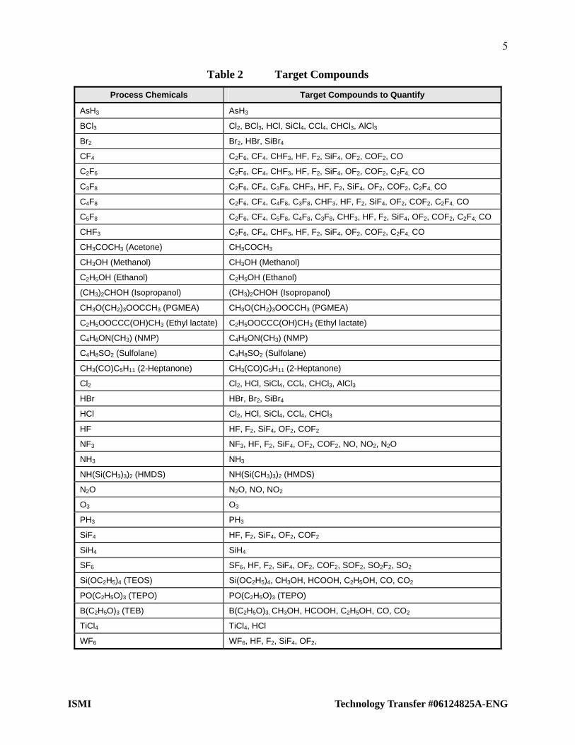
4 TARGET GASEOUS EMISSIONS The following list and table show which emission compounds should be quantified for a particular process chemical. Table 2 was designed as a guide for equipment suppliers; however, it may not list all the chemicals or ions that may be encountered with a specific tool and/or process, since many novel materials are continuously being introduced for the advanced technology nodes. A block flow diagram describing inputs and outputs to the process equipment and POU abatement device (if applicable) can help track all substances entering and leaving the tool and abatement device.

• The following target compounds should be quantified using calibration standards: NF3, C3F8, C2F6, CF4, C4F8, SF6, CHF3, C5F8, CH3OH (methanol), C2H5OH (ethanol), CH3COCH3 (acetone), (CH3)2CHOH (isopropanol), NH(Si(CH3)3)2 (HMDS), C2H5OOCCC(OH)CH3 (Ethyl lactate), C4H6ON(CH3) (NMP), CH3O(CH2)3OOCCH3 (PGMEA), C4H8SO2 (Sulfolane), CH3(CO)C5H11 (2-Heptanone), HF, Cl2, HCl, F2, SiF4, OF2, CO, NO, NO2, N2O, NH3, and SO2.

• BrCl should be measured when Br- and Cl-containing compounds are part of the process recipe

• During emissions testing, a survey scan must be taken. If any unidentified intensities are 10% of the height of the most intense peak attributed to a process gas, then the source of that peak needs to be identified and quantified.

• If FTIR analysis is ineffective in determining NO or NO2 emissions, then chemiluminescence methods can be used to quantity the emissions.

5


Table 2 Target Compounds

Process Chemicals Target Compounds to Quantify

AsH3 AsH3

BCl3 Cl2, BCl3, HCl, SiCl4, CCl4, CHCl3, AlCl3

Br2 Br2, HBr, SiBr4

CF4 C2F6, CF4, CHF3, HF, F2, SiF4, OF2, COF2, CO

C2F6 C2F6, CF4, CHF3, HF, F2, SiF4, OF2, COF2, C2F4, CO

C3F8 C2F6, CF4, C3F8, CHF3, HF, F2, SiF4, OF2, COF2, C2F4, CO

C4F8 C2F6, CF4, C4F8, C3F8, CHF3, HF, F2, SiF4, OF2, COF2, C2F4, CO

C5F8 C2F6, CF4, C5F8, C4F8, C3F8, CHF3, HF, F2, SiF4, OF2, COF2, C2F4, CO

CHF3 C2F6, CF4, CHF3, HF, F2, SiF4, OF2, COF2, C2F4, CO

CH3COCH3 (Acetone) CH3COCH3

CH3OH (Methanol) CH3OH (Methanol)

C2H5OH (Ethanol) C2H5OH (Ethanol)

(CH3)2CHOH (Isopropanol) (CH3)2CHOH (Isopropanol)

CH3O(CH2)3OOCCH3 (PGMEA) CH3O(CH2)3OOCCH3 (PGMEA)

C2H5OOCCC(OH)CH3 (Ethyl lactate) C2H5OOCCC(OH)CH3 (Ethyl lactate)

C4H6ON(CH3) (NMP) C4H6ON(CH3) (NMP)

C4H8SO2 (Sulfolane) C4H8SO2 (Sulfolane)

CH3(CO)C5H11 (2-Heptanone) CH3(CO)C5H11 (2-Heptanone)

Cl2 Cl2, HCl, SiCl4, CCl4, CHCl3, AlCl3

HBr HBr, Br2, SiBr4

HCl Cl2, HCl, SiCl4, CCl4, CHCl3

HF HF, F2, SiF4, OF2, COF2

NF3 NF3, HF, F2, SiF4, OF2, COF2, NO, NO2, N2O

NH3 NH3

NH(Si(CH3)3)2 (HMDS) NH(Si(CH3)3)2 (HMDS)

N2O N2O, NO, NO2

O3 O3

PH3 PH3

SiF4 HF, F2, SiF4, OF2, COF2

SiH4 SiH4

SF6 SF6, HF, F2, SiF4, OF2, COF2, SOF2, SO2F2, SO2

Si(OC2H5)4 (TEOS) Si(OC2H5)4, CH3OH, HCOOH, C2H5OH, CO, CO2

PO(C2H5O)3 (TEPO) PO(C2H5O)3 (TEPO)

B(C2H5O)3 (TEB) B(C2H5O)3, CH3OH, HCOOH, C2H5OH, CO, CO2

TiCl4 TiCl4, HCl

WF6 WF6, HF, F2, SiF4, OF2,

6


5 EMISSIONS CHARACTERIZATION

Worksheet #1 – General Information, of the Data Collection Template, describes the tool, the process being run by the tool, and the POU abatement device. It should document the following information: Type of tool tested

• Name of the baseline process, name/model of the tool, description of the process function (e.g., “deposits 1000 Å of an oxide film”)

• Batch or single-wafer tool, wafer throughput, wafer size

The report accompanying the Data Collection Template should document the following information for each analytical method used and the instrumentation parameters involved:

• The analytical methods used

• Who performed the testing (in-house or third-party ); provide a contact number for technical questions

• Mass or wave number range; detection limits of the instrumentation for each of the analyte compounds

• Type and model name of the instrument used

• The sampling conditions for calibration and monitoring (source pressure, electron energy, sampling frequency, detection method and settings [Faraday or multiplier], etc.)

The tool baseline recipe should be used as the basis for the tool environmental characterization. Emission data should be averaged over at least five wafers. The average for the five wafers and the standard deviation should be reported. Data should be collected for all activities associated with the tool:

• During wafer processing

• While no wafers are being processed (i.e., tool is idling or on stand-by)

• During the dry chamber clean

• During preventive maintenance

6 TEST FOR AIR EMISSIONS

6.1 Process Recipe The equipment supplier’s baseline process recipe must include flows, times, radio frequency (RF) power, plasma pressure, and spin speed. All sub-steps to the process should be included. For example, most etching recipes consist of a stabilization, etch, and over-etch step. The process parameters (flows, times, etc.) listed previously should be determined for each of the sub-steps.

7


6.2 Pump Purge Estimation The pump purge rate on the process tool must be determined when sampling the process exhaust downstream of the pump. Accepted methods of determining pump purge rates can be found in the mass spectrometry protocol described in Appendix A.1.4. Note: The pump purge rate can also be estimated using FTIR and a tracer gas such as SF6.

6.3 Calibration Curves Plots of signal intensity vs. analyte concentration must be provided for each of the compounds. The slope (with error), y intercept, and correlation coefficients must be provided with each plot. Figure 1 shows an example of a typical calibration curve. The error associated with the slope must not exceed 5%. The calibration curve should consist of at least 1 point per factor of 10 and no less than 5 points.

-2000 0 2000 4000 6000 8000 10000 12000

0

1

2

3

4

5

6

7slope = 0.00052 ± 0.00001y-int. = 0.10 ± 0.06

R2 = 0.9988

Inte

nsity

(a.u

.)

Concentration (ppm)

Figure 1 Sample Calibration Curve

6.4 Emission Values If the process tool uses a plasma, then both the concentration (ppmv) vs. time plots for the no RF and wafer processing experiments must be included. Figure 2 illustrates how the concentration (ppmv) vs. time plots should be plotted. All final emission values must be expressed in g/wafer. The equation used to derive the g/wafer value from the raw signal intensities must be included. To allow a semiconductor company to relate the emission values obtained from the tool supplier to its particular process, a statistical design of experiments (DOE) must be conducted for chemical flow, RF power (if applicable), and plasma pressure (if applicable). For process tools that use spin coaters, spin speed should be one of the variables used in the DOE. If the DOE cannot be completed (i.e., insufficient resources), then the baseline recipe alone should be tested. All baseline emission values should be the average of at least five wafers or five group of wafers

8


processed (i.e., a group could be a rack of wafers or a few racks of wafers during a process run). The average as well as the standard deviation should be reported. The error in the average must not exceed 10%. If a specific compound is not detected, then the detection limit of the instrumentation for that compound should be given. How the detection limit was determined should also be clearly explained.

15:25:00 15:30:00 15:35:00 15:40:00 15:45:00 15:50:00

0

500

1000

1500

2000

2500

Con

cent

ratio

n (p

pmv)

Time

Figure 2 Example of Process Emission Plots

6.5 Volume Closure From the equivalent halide inlet and outlet amounts, a volume closure on the halogens (F, Cl, Br) must be calculated. The equivalent halide outlet (EHO) is calculated by Eq. [1]: EHO (A) = Volume emitted of compound (A) × number of halides in compound (A) Eq. [1]

Similarly the equivalent halide inlet (EHI) is calculated by Eq. [2]: EHI (A) = Volume of process compound used for compound (A) (from recipe) Eq. [2] × number of halides present in compound (A)

The volume closure is then calculated by Eq. [3]: Volume closure = (total amount of EHO/total amount of EHI) × 100% Eq. [3]

Note that the total amount of EHO or EHI is merely the sum of the EH for all compounds that are either emitted (outlet) or used (inlet) in the process.

– Example: A process recipe of 50 sccm (0.05 slpm) of CF4 for 60 sec emits 30 scc (0.03 std. liters) of HF and 40 scc (0.04 std. liters) of CF4.

– Total EHI = 0.05 slpm × 1 min.× 4 Fluorine equivalents in CF4 = 0.20

9


– Total EHO = (0.03 × 1 Fluorine equivalent in HF) + (0.04 × 4 Fluorine equivalents in CF4) = 0.03 + 0.16 = 0.19

– Fluorine Volume closure = 0.19/0.20 × 100 = 95%

The success criterion for volume closure is greater than 90%. If the volume closure for volatile emissions is less than 90%, a plausible explanation and supporting data must accompany the report. Some possible reasons for a low volume closure are 1) solids formation, 2) unquantified volatile emissions, or 3) liquid emissions. For example, if the equipment supplier gets a 60% volume closure for a specific process and believes it is due to solids formation, then the supplier must identify the composition of the solids.

Volume closure for additional constituents should be provided, as applicable.

6.6 Chemical Utilization Efficiency If the process tool uses plasma, the utilization efficiency (UE) for a specific process compound must be calculated by two methods: Method #1 and Method #2. If the process tool does not use a plasma source, then only Method #2 needs to be used. The calculation for both methods is as follows.

• Method #1 (for process equipment that uses plasma) Method #1 uses the values from concentration vs. time plots (i.e., the raw concentrations have not been converted into grams per wafer).

Utilization Efficiency = 1 – [average concentration of process compound emitted1/average concentration process compound input2] × 100%.

• Method #2 (for any process equipment) Utilization Efficiency = 1 – [mass of process compound emitted3/mass of process compound used4] × 100%; where

1. This value is the average concentration for a single wafer for the emitted process compound from the “wafer processing” concentration vs. time plot (Figure 2).

2. This value is the average concentration for a single wafer for the emitted process compound from the “no RF experiment” concentration vs. time plot (Figure 2).

3. This value is the mass of emitted process compound for a single wafer (g/wafer), which is calculated by converting the average concentration using the gas flow rate.

4. This value is the mass of process compound for a single wafer (g/wafer) used as calculated from the process recipe.

6.7 Process Tools Using Open/Covered Tanks/Baths

There are additional testing concerns when characterizing the emissions of process tools that contain open/closed tanks/baths. The sampling point for the emissions characterizations should be downstream of the process tool (i.e., somewhere on the exhaust manifold of the tool). Because the emissions from these types of tools are continuous, testing must be completed when the wafer is processing and when the tool is idle. Furthermore, because data suggest that the emissions from these tools depend on how many wafers are on the rack, these test must be conducted using full racks of wafers. The emissions should be reported in terms of g/wafer and

10


mass per unit time. The emission values should be the average of at least five racks of wafers. The equipment supplier must also clearly indicate how many wafers are in a rack (e.g., 25 wafers, 50 wafers, etc.).

6.8 Spray Processes Spray processes are defined in this document as a process that dispenses chemical onto a wafer (single-wafer tool) or group of wafers (including racks of wafers). The chemical (e.g., acid solutions, base solutions, and organic compounds) can be dispensed onto a wafer or rack of wafers through an applicator or can be sprayed on. Air emissions can be measured in the exhaust duct from the spray chamber or application area. Liquid drains can be segregated based on type of wastewater or solvent waste. Data should be determined for five separate runs, with a run consisting of total use of all chemicals in the process.

6.9 POU Abatement Device DRE Testing DRE testing of POU abatement devices should be conducted using proper analytical techniques simultaneously on the inlet and the outlet locations. Testing should be conducted during all processes including wafer processing and dry chamber cleans. Detailed instructions for sampling inlet and outlet locations of POU abatement devices are in Appendix B.

Any dilution effects in the POU abatement device (i.e., addition of nitrogen, air, etc. to POU abatement device) must be removed in DRE calculations. DRE calculated on a mass basis will remove any dilution affects. It is calculated as follows:

• % DRE = [(mass in – mass out)/(mass in)] × 100%

DRE should not be calculated using inlet and outlet concentrations [e.g., parts per million by volume (ppmv)] without considering the dilution factor. DRE calculated on a concentration basis using dilution factor is as follows:

• % DRE = {[inlet ppmv – (outlet ppmv × dilution factor)]/(inlet ppmv)} × 100%

where the dilution factor is the ratio of total outlet gas flow rate divided by total inlet gas flow rate (i.e., dilution factor = outlet gas flow rate/inlet gas flow rate with the gas flow rate expressed in standard liters per minute, where standard refers to 25°C and one atmosphere pressure).

7 TEST FOR LIQUID EFFLUENTS To facilitate the understanding the liquid inputs and outputs from the tool or POU abatement device, including a block diagram in the emissions report is recommended. The data for all liquid effluents generated by the tool or POU abatement device during its operation must be entered into Worksheet #3. This includes any liquid effluent resulting from any “tank pickling” operation (i.e., chemical(s) used to flush and condition the chemical bath before introducing the chemical used for processing).

11


7.1 Block Diagram Showing Connections to Tool The equipment supplier should provide a block diagram that clearly shows all the points of connection to the process tool, both input chemicals and output liquid chemicals and wastewater The type of drain should be labeled (i.e., solvent drain, acid wastewater drain, fluoride wastewater drain, etc.). Also the identity and concentrations of the primary constituents of the input streams and outputs streams (drains) should be included.

Specific information is required for each point of connection (whether it be input chemical/water or output chemical/wastewater/waste). Each point of connection should be assigned a number and purpose.

• Example: Connection point #1 is the input ultrapure water (UPW). Its purpose is to supply UPW to the process tool for wafer rinsing.

• Example: A process tool with four connection points (three inputs [chemicals] and one output [drain]) is shown in Figure 3.

ProcessTool

UPW

H2SO4

HCl

Acid Drain (100 ppmH2SO4, 50 ppm HCl)

Input Output

Figure 3 Connection Hookup Diagram

7.2 Chemical/Water Inputs and Effluents The volume associated with each connection point must be included. If the chemical/water flows through the tool, then the volume should be quantified in liters per minute (lpm). For tools with continuous flows, an average flow rate, a maximum flow rate, and an idle flow rate along with an associated time per wafer for each of the flows are required. If the chemical/water is used in a static bath, then the volume should be expressed in liters and the dump frequency specified. If the connection point is a drain, then the outlet flow rate of the chemicals/wastewater should be included. Finally, the primary constituents should be identified and quantified for each of the output connection points (drains). All concentrations should be the average of at least five cycles. Both the average and standard deviation should be included. Accredited, standard testing methods such as listed in Appendix C must be used for sampling and analysis of all liquid effluents.

8 SOLID WASTE GENERATED DURING WAFER PROCESSING The equipment supplier must identify any solid waste generated during wafer processing or operation of the abatement device. The supplier must identify the composition and the quantity of solid waste generated in g/wafer and must enter it in Worksheet #4. Accredited, standard testing methods such as listed in Appendix C must be used for sampling and analysis of all solid wastes. All emissions should be the average of at least five cycles. Both the average value and standard deviation should be included. Consumables such as CMP pads, filter cartridges,

12


sputtering targets, etc., are solid waste items that are captured in Worksheet #5 under Preventive Maintenance.

9 EMISSIONS ASSOCIATED WITH PREVENTIVE MAINTENANCE (PM) Air emissions, liquid effluents, and solid waste associated with preventive maintenance (PM) activities on the process tool or abatement device are captured on Worksheet #5. In addition to the air, liquid, and solid emissions, the tool supplier must record the use of any post-PM flushing chemical(s), all consumables, and PM-associated parts cleaning data on this worksheet. All the emissions generated during the PM activities must be added to the other tool air emissions, liquid effluents, and solid waste (Worksheets #2, #3, and #4) to arrive at total mass emissions per wafer, which are summarized in Worksheet #6.

10 DATA COLLECTION TEMPLATE The data collection template consists of an Excel-based workbook with six separate worksheets as follows:

• Worksheet #1 – General Information (about the tool)

• Worksheet #2 – Air Emissions

• Worksheet #3 – Liquid Effluents

• Worksheet #4 – Solid Wastes

• Worksheet #5 – Preventive Maintenance

• Worksheet #6 – Data Summary

Worksheet #6 is a compilation of the information from the other worksheets. This summary will help the semiconductor manufacturer review environmental emissions on a per wafer basis. If mass per unit time data are needed, they can be found in other worksheets.

The soft copy version of the spreadsheets allow the supplier to add and expand rows and columns, as necessary, for the full environmental characterization of a particular tool.

13


Worksheet #1 – General Information

Instructions The template consists of the following six worksheets:

1. Worksheet #1 asks for General Information (about your tool)

2. Worksheet #2 pertains to Air Emissions

3. Worksheet #3 pertains to Liquid Effluents

4. Worksheet #4 pertains to Solid Waste

5. Worksheet #5 pertains to Preventive Maintenance

6. Worksheet #6 is a Data Summary of the data provided in Worksheets #1–#5 (please consult before you start)

• Please review all six worksheets and provide all information that applies to your specific tool.

• For the reader's convenience, please identify the tool name and tool model on each worksheet.

• Please provide all data in metric units.

• Please provide explanations or any additional information in the Comments column, where applicable.

• Before you start, please check Worksheet #6 – Data Summary to see what data is asked for

• Please indicate how the data was obtained (in-house or by 3rd party) and what analytical techniques were used in the summary report accompanying this workbook

General Information

Date (form was filled out)

Contact Name (telephone #)

Wafer Size

Single Wafer Tool (yes/no)

# of Wafers/Batch

Chamber Clean (in situ or remote)

Supplier Name

Tool Name/Model

Process Name

Batch Tool (yes/no)

Design Throughput (wafers/hr)

Type of Film Deposited/Etched/Cleaned

ISMI Technology Transfer #06124825A-ENG 14

Worksheet #2 – Template for Reporting Process Air Emissions

Tool Name: Baseline Deposition or Etch Recipe Information (Repeat for Clean Recipe and Seasoning Recipe, if applicable)

Parameters/Steps Step 1 Step 2 Step 3

Time (sec)

Pressure (Torr)

RF Power (W)

Flow of A (sccm)

Flow of B (sccm)

Flow of C (sccm)

etc. [3]

1.0 Processes such as PVD, CVD, etch, implant, etc.

1.1 Emissions During Wafer Processing

Input Chemical Volume In (scc/wafer)

Mass In (g/wafer) Mass In (g/hr) Comments

A

B

C

etc. [3]

Chemical Emitted Volume Out (scc/wafer)

Mass Out (g/wafer)

Mass Out (g/hr)

Utilization[1] (%)

Utilization[1] (std. dev.) Comments

A

B

C

etc. [3]


Worksheet #2 – Template for Reporting Process Air Emissions (continued)

1.2 Emissions During “Dry” Chamber Clean

Input Chemical Volume In (scc/wafer)

Mass In (g/wafer)

Mass In (g/hr) Comments

A

B

C

etc. [3]

Chemical Emitted Volume Out (scc/wafer)

Mass Out (g/wafer)

Mass Out (g/hr)

Utilization[1] (%)

Utilization[1] (std. dev.) Comments

A

B

C etc. [3]

1.3 Process Component Volume Closure (i.e., halides, NH3, P, etc.)

Component In

During Wafer

Processing (scc/wafer)

During Chamber

Clean (scc/wafer)

Total Volume In (scc/wafer)

Total Mass In (g/wafer) Comments

F

Cl

Br

etc. [3]

Component Out

During Wafer

Processing (scc/wafer)

During Chamber

Clean (scc/wafer)

Total Volume Out (scc/wafer)

Total Volume

Closure[2] (%)

Volume Closure[2] (std. dev.)

Total Mass Out

(g/wafer) Comments

F

Cl

Br

etc. [3]



1.4 Emissions During Tool Idle (e.g., periodic chamber cleans when wafers are NOT being processed)

Input Chemical Mass In (g/hr) Comments

A

B

C etc.[3]

Chemical Emitted Mass Out

(g/hr) Utilization[1]

(%) Utilization[1] (std. dev.) Comments

A

B

C

etc. [3]

2.0 Emissions from Wet Stations/Benches

Tank Chemical

Used Comp. (%)

Tank Volume (liters) Temp. (ºC)

Does tank have a cover?

(yes/no)

% of Time Chemical is

in Tank

Type of Agitation

(e.g., sparge,

megasonic) Comments

a

b

c

etc. [3]



2.1 Emissions for Tank "a" (repeat for each tank)

Chemical Emitted

Avg. Emissions w/o Wafers

(g/hr) Avg. Emissions During Wafer Processing (g/hr)

Avg. Emissions per Wafer Processed (g/wafer)

Avg. Process Exhaust Volume

(m3/hr) [4]

Average Concentration in Process Exhaust During

Dispense (ppmv) Comments

A

B

C

etc. [3]

3.0 Emissions from Spray Processors

Input Chemical Comp. (%) Flow Rate

(sccm) Duration of Flow (sec) Temp. (°C)

% of Recipe Time

Chemical is Applied Comments

A

B

C

etc. [3]

Chemical Emitted

Average Emissions for Each

Wafer Processed (g/wafer)

Average Emissions

During Dispense

(g/sec)

Average Process Exhaust Volume

(m3/hr) [4]

Average Concentration in Process Exhaust During

Dispense (ppmv) Comments

A

B

C

etc. [3]

Notes: [1] = % utilization = (mass in – mass out)/mass in × 100%. [2] = % volume closure = volume out/volume in × 100%. [3] = List all chemicals used as well as any byproducts formed. [4] = 1 cfm = 1.7 m3/hr

Remarks: 1. Please list the analytical method(s) used to obtain the data. 2. Provide a copy of the 3rd party test report(s), where applicable. 3. Provide a simplified process flow diagram showing all the streams entering and leaving the tool.


Worksheet #3 – Template for Reporting Liquid Effluents

Tool Name:

3.0 Specific Information

# of connections per tool

# of recirculation loops

drain interlocks (yes/no)

drain switching capability (yes/no)

drain switching capability (manual/auto)

3.1 Chemical / DI Water / Wastewater /Solvent Effluent

Input Chemical / Solvent / DI Water / Purpose

Time for Step (sec)

Chemical Constituent

[2] Concen. (mg/L)

Avg. Flow [1]

(lpm)

Maximum Flow [1]

(lpm)

Idle Flow [1]

(lpm) Volume

(lpm)

Total Volume

(ltrs/step)

Spiking Amount (% & ltrs/hr) Comments

Step 1 A

B

C

Step 2 A

B

C

Step 3 A

B

C

Effluent / Drain Time for

Step (sec)


[2] Concen. (mg/L)

Avg. Flow [1]

(lpm)

Maximum Flow [1]

(lpm)

Idle Flow [1]

(lpm)

Bath Discharge

Volume (ltrs/step)

Bath Discharge Frequency

(#/week) Comments

Step 1 A

B

C

Step 2 A

B

C


Worksheet #3 – Template for Reporting Liquid Effluents (continued)

Effluent / Drain Time for

Step (sec)


[2] Concen. (mg/L)

Avg. Flow [1]

(lpm)

Maximum Flow [1]

(lpm)

Idle Flow [1]

(lpm)

Bath Discharge

Volume (ltrs/step)

Bath Discharge Frequency

(#/week) Comments

Step 3 A

B

C

3.2 Tank Pickling Chemistry [3]

Drain


[2] Concen. (mg/L)

Flow [1] (lpm)

Total Volume

(ltrs) Duration

(min) Frequency (#/month) Comments

A

B

C

Note: [1] Averaged over 5–10 wafer processing cycles. [2] Constituents of high interest: NH3, SO4, F, Cu, TSS, organic compounds in water. [3] Refers to chemical used to flush and condition the chemical bath prior to introducing the chemical used for processing.

Remarks: 1. Please list the analytical methods used to obtain the data. 2. Provide a copy of the 3rd party test report(s), where applicable. 3. Provide a simplified process flow diagram showing all the streams entering and leaving the tool.

20


Worksheet #4 – Template for Reporting Solid Waste

Tool Name/Model:

4.0 Solid Waste Produced during Wafer Processing (see 5.5 Consumables on Worksheet 5 as well)

Type of Waste

Total Waste Generated (kg/24 hrs)

Frequency (if intermittent)

Amount Generated (g/wafer)

Chemical Constituent(s)

Concentration (wt%) Comments

A

B

C



Worksheet #5 – Template for Reporting Preventive Maintenance (PM) Emissions

Tool Name/Model:

5.0 General

Description of procedure

Frequency of procedure

Time between PMs (hrs)

Number of wafers between PMs

Estimated length of procedure

5.1 Air Emissions

Chemical Amount Used

(g/proc.) Constituent Constituent Concen. (%)

Mass Emitted (g/proc.)

Total Mass (g/wafer) Comments

A

B

C

5.2 Liquid Chemical/Wastewater Emissions

Chemical Amount Used

(ltrs/procedure) Constituent

Constituent Concentration

(%) Total Mass

(g/procedure) Total Mass (g/wafer) Comments

A

B

C

5.3 Solid Waste Generated

Solid Waste Amount

(g/procedure) Constituent

Constituent Concentration

(%) Total mass (g/wafer) Comments

A B C


Worksheet #5 – Template for Reporting Preventive Maintenance (PM) Emissions (continued)

5.4 Qualification after PM

Flushing Chemical Volume Used (g/procedure) Constituent

Concentration (%)

Air Emissions (g/procedure)

Liquid Waste (g/procedure)

Solid Waste (g/procedure) Comments

A B C

5.5 Consumables

Frequency of Replacement # Wafer Passes Hours of Use Quantity

Contaminated? Yes/No

Contaminating Constituent(s) Comments

Anodes and Cathodes Targets CMP Pads Post-CMP Brushes Filters Batteries Lamps Grease Ionizer Bar Emitter Tips

Contaminated Wipes


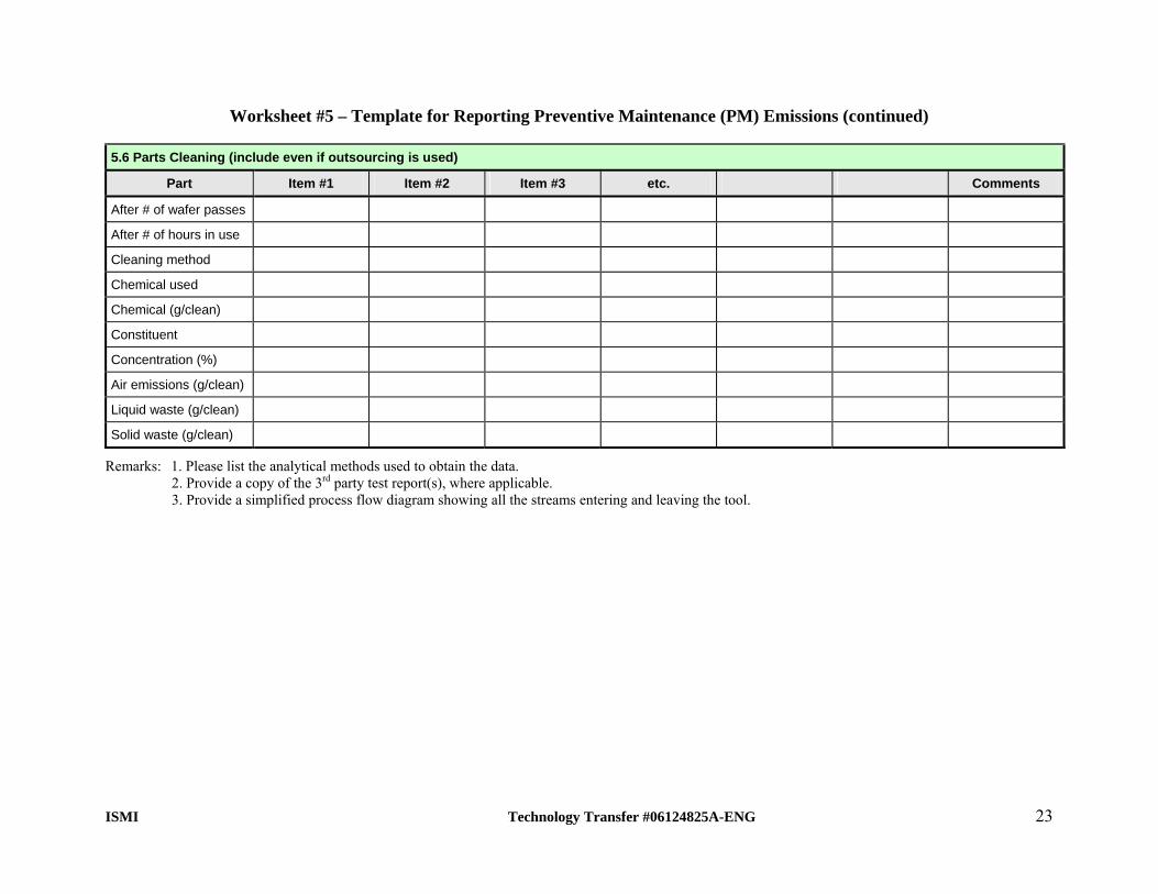
Worksheet #5 – Template for Reporting Preventive Maintenance (PM) Emissions (continued)

5.6 Parts Cleaning (include even if outsourcing is used)

Part Item #1 Item #2 Item #3 etc. Comments

After # of wafer passes

After # of hours in use

Cleaning method

Chemical used

Chemical (g/clean)

Constituent

Concentration (%)

Air emissions (g/clean)

Liquid waste (g/clean)

Solid waste (g/clean)


24


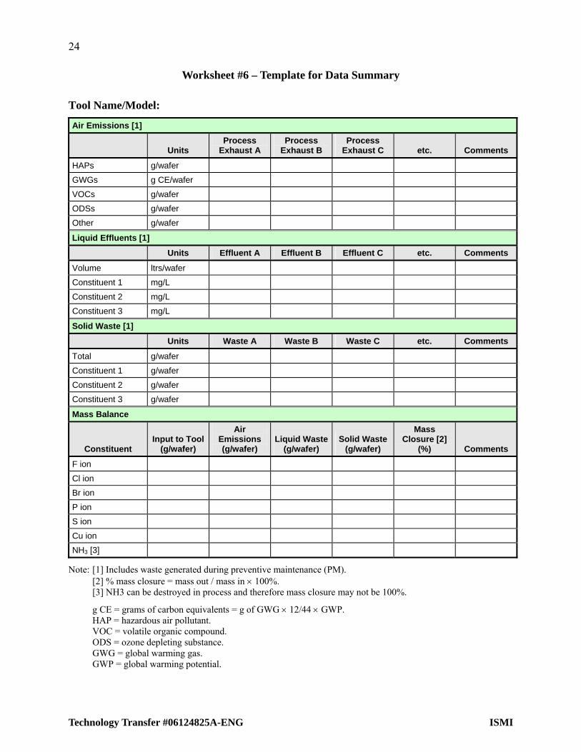
Worksheet #6 – Template for Data Summary

Tool Name/Model:

Air Emissions [1]

Units Process

Exhaust A Process

Exhaust B Process

Exhaust C etc. Comments

HAPs g/wafer

GWGs g CE/wafer

VOCs g/wafer

ODSs g/wafer

Other g/wafer

Liquid Effluents [1]

Units Effluent A Effluent B Effluent C etc. Comments

Volume ltrs/wafer

Constituent 1 mg/L

Constituent 2 mg/L

Constituent 3 mg/L

Solid Waste [1]

Units Waste A Waste B Waste C etc. Comments

Total g/wafer

Constituent 1 g/wafer



Mass Balance

Constituent Input to Tool

(g/wafer)

Air Emissions (g/wafer)

Liquid Waste (g/wafer)

Solid Waste (g/wafer)

Mass Closure [2]

(%) Comments

F ion

Cl ion

Br ion

P ion

S ion

Cu ion

NH3 [3]

Note: [1] Includes waste generated during preventive maintenance (PM). [2] % mass closure = mass out / mass in × 100%. [3] NH3 can be destroyed in process and therefore mass closure may not be 100%.

g CE = grams of carbon equivalents = g of GWG × 12/44 × GWP. HAP = hazardous air pollutant. VOC = volatile organic compound. ODS = ozone depleting substance. GWG = global warming gas. GWP = global warming potential.

25


APPENDIX A – TECHNICAL PROTOCOLS FOR AIR EMISSIONS CHARACTERIZATION

This appendix explains the best known methods for conducting air emissions studies. While other analytical methods may be applied to air emissions characterization, most of these techniques have severe limitations and more supporting data must be provided to guarantee the quality of the data. The three recommended techniques for conducting the air emissions studies are mass spectrometry (MS), FTIR, and fluorine chemiluminescence. The MS protocol was written by Air Products and Chemicals Inc.; the FTIR protocol was written by 3M Corporation; and the fluorine chemiluminescence protocol was written by URS.

A.1 Mass Spectrometry Protocol Mass spectrometry is the standard quantitative analytical method for the determination of CF4, C2F6, C3F8, CHF3, NF3, and SF6 in process tool exhaust streams.

A.1.1 Introduction This procedure was developed to determine CF4, C2F6, C3F8, CHF3, NF3, and SF6 found in semiconductor processing effluent streams. These compounds are primarily found in the effluent of chemical vapor deposition (CVD) and plasma etch applications. The method is based on using quadrupole mass spectroscopy (QMS). In QMS, the sample is ionized using electron impact ionization. The quadrupole mass filter separates the ions based on their mass-to-charge ratio (m/e). A secondary electron multiplier or a Faraday plate is used as a detector for these mass separated ions. Concentrations of the individual components in the sample are determined from QMS response factors, which are determined from direct calibration of the QMS response to the compounds listed above.

• Basic QMS Configuration The basic components of a quadrupole mass spectrometer system are an ionizer, a quadrupole mass filter, and a detector such as an electron multiplier.

• Ionizer Here the molecules in the sample gas are ionized. Thermionic emission from tungsten or thoriated iridium filaments are used to produce 70 eV electrons. These electrons can ionize the molecules by the following interaction:

e- + ABC → ABC+* + 2e-

ABC+* → A + C+ B+

→ AB+ + C

The molecule ABC is first ionized into an excited ionic state. Depending upon the structure of the molecule, the excited ionic state will produce different fragment ions of the type AB+, B+, AC+, etc.

The ions produced in the ionizer are extracted using an electrostatic lens. A series of electrostatic lenses are used to focus the extracted ions into the entrance of the quadrupole mass filter.

26


• Quadrupole Mass Filter (QMF) The QMF consists of four cylindrical rods to which both RF and DC voltages are applied. The rods opposite each other are connected together. The voltage + (U + Vcosωt) is applied to one set of rods, whereas the voltage -(U + Vcosωt) is applied to the other set of rods. The typical operating frequency of the RF voltage is 1.2 MHz. Under the influence of this quadrupolar field, the equation of motion for the ions is represented by the Matheiu equation:

( )d ud

qq

2

2 2 2ζ

ζ + a u = 0u − cos Eq. [A-1]

where: ζω

= t

2 Eq. [A-2]

and aeU

m ru =4

2 2ω Eq. [A-3]

where U is the DC voltage, m is mass, ω is angular frequency, and r is the radius of the quadrupole and

qeV

m ru =2

2 2ω Eq. [A-4]

where V is the peak amplitude of the RF voltage of angular frequency ω.

The solutions to the Matheiu equation fall into either stable or unstable regions, depending upon the mass-to-charge ratio of the ion. The ions for which the solution is stable exit the quadrupole, whereas all other ions have unstable trajectories and hit the rods of the quadrupole. By changing the amplitude of the RF field (V) different ions can be made to have stable trajectories. Thus by changing the RF field, the QMS can be tuned to transmit different masses. The resolution of the QMF is determined by the ratio U/V. For constant resolution, the ratio U/V is kept constant when the RF voltage is adjusted to change the transmitted mass.

• Detection System

The ions transmitted by the QMF are detected using either a Faraday plate or an electron multiplier. The Faraday plate is a metal plate placed at the end of the quadrupole filter. A sensitive electrometer connected to this plate records the current produced when a charged ion hits the Faraday plate. Typically, the electrometer is sensitive enough to detect current in the pico ampere range.

For currents smaller than a few pico amperes, an electron multiplier is used instead of the Faraday plate. In most QMSs, a continuous dynode electron multiplier is used although a discrete dynode electron multiplier could also be used. The entrance of the electron multiplier is biased at about -2000 V, whereas the other end is connected to a ground-referenced amplifier. The positive ions exiting the quadrupole are accelerated towards the -1500 V potential on the entrance of the electron multiplier. When the ions strike the electron multiplier, they generate a few secondary electrons. These secondary electrons, under the influence of the gradient in the electron multiplier, strike a different part of the electron multiplier. Each electron produces a few secondary electrons. These electrons will cascade down the electron multiplier. This cascading effect generates about a million

27


electrons for every ion that strikes the entrance of the electron multiplier. This enhanced signal is measured by the preamplifier.

• QMS Resolution A QMS is normally operated in a unit mass resolution mode meaning masses are separated by one atomic mass unit. The resolution of a QMF is defined by the equation:

m/Δm = (0.126)(0.1678 - U/V)-1 Eq. [A-5]

For infinite resolution, U and V are given by the equations: U (volts) = 1.212 mf2r2 Eq. [A-6]

V (volts) = 7.219 mf2r2 Eq. [A-7]

where f is frequency. Resolution (m/Δm) can be empirically determined by dividing the center point mass by the full width at half height of the peak for each mass of interest.

• Detection Limits

The mass spectrometer chosen for this application should have the necessary sensitivity to detect the selected effluent species at a predetermined level. The typical detection limit of each component determined with the QMS used for this study was 1–10 ppmv. System detection limits can be calculated using SEMI guideline F33-0998, which describes the calculation of a regression-based limit of detection. Two regression-based means for determining a limit of detection (LOD), ordinary least squares (OLS) and weighted least squares (WLS) are often used. OLS analyses implicitly assume that signal variability is the same everywhere within the calibration window. WLS analyses allow signal variability to vary over the calibration window, but require an appropriate set of weights to complete the analysis. The LOD is calculated to obtain a 3 σ equivalent (in probability) upper confidence limit. PC-based software is available from Air Products to help calculate statistical LODs based on the SEMI guideline.

A.1.2 Sampling Conditions

• Sampling Location The sample is taken downstream of the process tool and pump package (see Figure A-1). The exact location is determined by the specific tool and piping configuration associated with the process. The sample exhaust is vented back into the corrosive house ventilation system at a point downstream of the sample inlet location.

• Sampling Conditions Perfluorocompound (PFC) utilization efficiencies should be determined during actual wafer processing. For etch applications, efficiencies should be determined while etching a wafer (WIP, dummy, or test). For chemical vapor deposition (CVD) applications, efficiencies should be determined during a chamber clean after deposition (efficiencies should not be determined in a clean chamber). All sampling is performed non-intrusively during wafer processing. Samples are drawn through the MS source by an external sample pump. The pressure in the exhaust is slightly below 1 atm. (~ 750 Torr). The pressure of the sample inlet is maintained at a lower pressure (~700–740 Torr) by throttling the sample pump. Because of the inertness of CF4, C2F6, C3F8, CHF3, NF3, and SF6, the sample lines do not need to be heated.

28


Calibration System

Corrosive Exhaust Line

From Process Tool 700 Torr

MassSpectrometer

P

SamplePump

Closed IonSource

To ProcessExhaust

Pump Exhaust

Figure A-1 Process Tool Exhaust Sampling System

• Mass Spectrometer Parameters Choice of specific QMS operating conditions such as electron energy, secondary electron multiplier voltage, emission current, and ion focusing voltage are left to the discretion of the analyst provided the QMS responses to analytes are calibrated under the same conditions. These parameters are systems-specific and will need to be determined by the analyst. To address questions in this area, analysts should consult the QMS manufacturer, the system manual, basic mass spectrometer textbook, and other such sources.

• Data Acquisition Mode For this application, the mass spectrometer is operated in the selective ion monitoring (SIM) mode. The ions chosen depend on the PFC(s) used in the process and the byproducts being monitored. Listed in Table A-1 are the fragment ions used to determine the PFCs typically in CVD and etch tool exhausts.

Table A-1 Monitored Fragment Ions

Compound Monitored Fragment Ion m/e

CF4 CF3+ 69

C2F6 C2F5+ 119

C3F8 C3F7+ 169

CHF3 CHF2+ 51

NF3 NF2+/NF3

+ 52/71

SF6 SF5+ 127

29


To identify unknown and known components in the sample, a complete mass spectrum is obtained by operating the mass spectrometer in the full spectrum scan mode. Standard mass spectra for each of the compounds listed above are in Figure A-2–Figure A-7. The spectra were obtained from the National Institute of Standards and Technology’s website.

100

80

60

40

20

0

20 40 60 80 100 120 140

Rel

. Abu

ndan

ce

m/z

Figure A-2 Mass Spectrum for Sulfur Hexafluoride (SF6)

100

80

60

40

20

0

10 20 30 40 50 60 80

Rel

. Abu

ndan

ce

m/z70

Figure A-3 Mass Spectrum for Nitrogen Trifluoride (NF3)

http://webbook.nist.gov/

30


100

80

60

40

20

0

10 20 30 40 50 60 80

Rel

. Abu

ndan

ce

m/z70

Figure A-4 Mass Spectrum for Trifluoromethane (CHF3)

100

80

60

40

20

0

20 30 45 60 75 90

Rel

. Abu

ndan

ce

m/z

Figure A-5 Mass Spectrum for Carbon Tetrafluoride (CF4)

31


100

80

60

40

20

0

0 40 80 120 160

Rel

. Abu

ndan

ce

m/z

Figure A-6 Mass Spectrum for Hexafluoro-Ethane (C2F6)

100

80

60

40

20

0

0 40 80 120 160 200

Rel

. Abu

ndan

ce

m/z

Figure A-7 Mass Spectrum for Octafluoropropane (C3f8)

32


• Flow Rates A sample flow rate of ~0.5–1.5 slm is drawn from the process tool exhaust stream under study. This typical flow rate is needed to purge the sample manifold and obtain a temporally representative sample of the process. The flow rate into the mass spectrometer source is ~10–20 sccm.

• Sample Frequency The required sample frequency depends on the process being monitored. The software of the mass spectrometer should be capable of capturing the data at the required sample frequency. Fast processes, such as etch processes, require rapid sampling frequencies. Typical etch sampling frequencies should be on the order of 0.33–1 Hz. CVD processes are longer and can tolerate sampling frequencies of 0.1– 0.33 Hz.

• Dynamic Dilution Calibration Parameters

The QMS must be calibrated for both mass location and response to analytes. A dynamic dilution calibration system is used to perform both types of mass spectrometer system calibrations. The simplest type of dynamic calibration system includes appropriate tubing, fittings, and two mass flow meters. One mass flow meter regulates the flow rate of the standard component used to calibrate the system. The second mass flow meter regulates the amount of diluent gas used to mix with the standard. The flow rates of the mass flow meters are adjusted to the appropriate settings to obtain the required concentrations for calibrating the MS. These data are used to generate a calibration curve for each compound of interest.

Mass flow controllers (MFCs) are used to accurately regulate the flow rates of the diluent and calibration gases. They should be calibrated using the single component gas being used with them. MFCs used with calibration mixtures should be calibrated with the calibration mixture balance gas if the individual components are ~2% or less. They should be calibrated over their range of use and operated in their experimentally determined dynamic linear range.

• Mass Location Calibration A mixture containing 1% He, Ar, Kr, and Xe in a balance gas of nitrogen is used to assure the alignment of the quadrupole mass filter. This mixture covers both low and high mass ranges. The mass spectrometer should be chosen so that the mass range is sufficient to detect the predominant peaks of the components under study.

• QMS Response Calibration The response of the QMS to the compounds listed above is determined by calibrating the system with test atmospheres containing the compounds of interest. These test atmospheres are created using dynamic phase dilution techniques as described above. A calibration curve should be generated for each compound.

• Calibration Frequency The mass spectrometer is calibrated before performing the first analysis of the day and after it is completed at the end of the day. This will enable the analysis to determine the drift of the instrument throughout the day.

33


• Calibration Range The mass spectrometer is quantitatively calibrated over the concentration range of the analysis for each gas to be analyzed. A multi-level calibration is performed using a minimum of five different concentrations including a zero. The zero point is defined as diluent containing no added analyte. The system should be calibrated over the concentration range of the samples.

A.1.3 Operating Procedures 1. Perform a qualitative mass calibration by running a standard containing stable components

that provide predominant signals at m/e values distributed throughout the mass range to be used. This will ensure the mass locations are properly identified and that the m/e values of the mass fragments are correctly identified.

2. Quantitatively calibrate the mass spectrometer system over the concentration range of each component in the sample that will be analyzed. The sample concentration should fall in the linear dynamic range of the mass spectrometer signal response. The calibration should be performed at the same mass spectrometer inlet pressure as when obtaining an effluent sample for analysis. One way to do this is to carefully regulate the inlet pressure using a throttle valve and monitor the pressure using a capacitance manometer. If this is not done, then the relationship between inlet pressure and signal response should be empirically determined on the mass spectrometer being used.

3. To determine the response time of the instrument to changes in a process, a process gas such as C2F6 should be turned on at the process tool for a fixed period of time. This should be a relatively short period (e.g., 20 sec). Then the amount of time it takes for the mass spectrometer to respond to this process gas should be recorded. This should be done at the beginning of each tool evaluation.

4. Pass the sample gas through the mass spectrometer, and acquire data for the required amount of time to track the process. The sample frequency is set to monitor the changes in the process. Repeat this for at least five wafers on the same process to obtain an average and standard deviation of process efficiencies and emission concentrations.

5. Repeat Step 2 above at the end of the day and more frequently if necessary.

A.1.4 Calculations

• Calibration Plot ion intensity vs. analyte concentration for a given compound obtained when calibrating the analytical system. Determine the slope and intercept for each calibrated species to obtain response factors with which to calculate concentrations in the sample. For an acceptable calibration, the R2 value of the calibration curve should be at least 0.98.

• Sample Analysis To determine the concentration of a specific component in the sample, divide the ion intensity of the sample response by the calibrated response factor. Repeat this for each component.

34


• Deconvolution of Interfering Peaks Interfering peaks must be deconvoluted to obtain accurate results. As an example of this, C2F6 and CF4 have common fragments in their mass spectra (CF3

+, CF2+, CF+, and F+). CF4

does not produce a fragment that is not observed in the mass spectra for C2F6. Thus the contribution of ions attributable to C2F6 must be deconvoluted from the ions attributable to CF4 at a common mass. Deconvolution can be achieved by using a prominent peak, such as C2F5

+, which is not common to both molecules. Contributions to m/e 69 from C2F6 can be subtracted by using the m/e 69/ m/e 119 ion intensity ratio obtained when C2F6 is present alone. For example, to determine the CF4 concentration in the presence of C2F6, the following expression can be used:

( )( ) B = 11962

69Total

694 FCCF SSS − Eq. [A-8]

( )( )C S RCF CF CF469

469

469 = Eq. [A-9]

where S is QMS signal, C is concentration, R is the response factor determine from the calibration curve, superscripts are amu values, and B is the branching ratio defined by

BC F2 6

69

119 C2F6

C2F6 SS

= Eq. [A-10]

If other compounds are present that contribute to the signal at m/e = 69, they must also be included in the calculation.

• Pump Purge Dilution To calculate the exhaust dilution factor, determine the concentration of the PFC in the effluent by turning the RF power in the chamber off and flowing the PFC at the process flow rate. Divide the process flow rate specified in slm by this determined concentration (specified as liter of analyte) to yield the pump purge dilution. This information can be used to estimate the emissions on a mass or volume basis (e.g., pounds per year or liters per years). Another way to determine this value is by using a mass flow controller or a velometer.

The calculation below shows an example of how to determine pump purge dilution. Assume 50 sccm of CF4 in the process tool yielded 500 ppmv average CF4 effluent concentration with the RF power off.

( )( )

( ) 1 1

46

1CF4 minL 100

L 10500

minL 050.0 −−−

−=

×FlowTotal

FlowTotalCF L Eq. [A-11]

Note that it is necessary to ensure RF power is off and that the compound chosen is thermally stable at the chamber temperature.

35


A.2 Fourier Transform Infrared (FTIR) Spectroscopy Protocol

Protocol for FTIR measurements of fluorinated compounds in semiconductor process tool exhaust. A.2.1 Introduction

This section provides procedural and quality assurance and quality control (QA/QC) bases for gaseous concentration measurements of fluorinated compounds by extractive FTIR spectrometry. The compounds of interest are SF6, NF3, C2F6, C3F8, CF4, and CHF3. They are to be measured in enclosed samples extracted from the effluent of semiconductor plasma tools; the analytes are typically in a mixture of oxygen and nitrogen with low moisture content (less than 0.1% by volume). Typical concentrations of the six analytes are in the 100–50,000 ppmv range. Because the tool effluent concentrations can change rapidly, measurements must be made at least twice per minute and several times per minute, if possible. This requirement places special emphasis on the sampling and data acquisition operations for this application.

Substantial field experience in the use FTIR spectroscopy gained in previous SEMATECH studies (see ref. [1] in Appendix A.2.9) was used in the preparation of this protocol. The nomenclature is adopted from ref. [2]. Appendix A.2.10 lists several salient definitions. The intended audience is the technical community familiar with plasma tool operation and standard emission testing methodologies. However, because FTIR spectrometry is a relatively new emissions testing technique, it is briefly described in Appendix A.2. Additional mathematical details of the technique are provided in Appendices A.2.7 and A.2.8.

A.2.2 Method Development The general procedure for developing and documenting an extractive, FTIR-based analysis of the effluent from semiconductor plasma tools is largely based on studies by SEMATECH and 3M Corporation.

Developing an FTIR method consists of two distinct phases: a laboratory study phase and 2) a field study phase. In practice, portions of these developmental phases may occur simultaneously, and some adjusts in the order and/or repetition of some activities may be necessary.

A.2.3 Laboratory Studies

• Proposed Spectroscopic Conditions

Propose a set of spectroscopic conditions under which the field studies and subsequent field applications are to be carried out. These include the minimum instrumental linewidth (MIL), spectrometer wavenumber range, sample gas temperature, sample gas pressure, absorption pathlength, maximum sampling system volume (including the absorption cell), minimum sample flow rate, and maximum allowable time between consecutive infrared analyses of the effluent.

• Criteria for Reference Spectral Libraries On the basis of previous emissions test results and/or process knowledge, estimate the maximum concentrations of the six analytes in the effluent and their minimum concentrations of interest (those concentrations below which the measurement of the compounds is of no importance to the analysis). Values between the maximum expected concentration and the minimum concentration of interest are referred to below as the

36


“expected concentration range.” Calculate the expected maximum absorbance level for each compound under the proposed spectroscopic conditions.

A minimum of four reference spectra must be available for each analyte. When the set of spectra is ordered according to absorbance, the absorbance levels of adjacent reference spectra should not differ by more than a factor of six. Optimally, reference spectra for each analyte should be available at absorbance levels which bracket the analyte’s expected concentration range; minimally, the spectrum must be available whose absorbance exceeds each analyte’s expected maximum concentration.

If reference spectral libraries meeting these criteria do not exist for all the analytes and interferants or cannot be accurately generated from existing libraries exhibiting lower MIL values than those proposed for the testing, prepare the required spectra according to the procedures below.

• Preparation of Reference Spectra When practical, pairs of reference spectra at the same absorbance level (to within 10%) of independently prepared samples should be recorded. The reference samples should be prepared from neat forms of the analyte or from gas standards of the highest quality commonly available from commercial sources. Either barometric or volumetric methods may be used to dilute the reference samples to the required concentrations, and the equipment used should be periodically calibrated in some independent fashion to ensure suitable accuracy. Dynamic and static reference sample preparation methods are acceptable, but dynamic preparations are more likely than static methods to give consistent results for reactive analytes. Any well characterized absorption pathlength may be employed in recording reference spectra, but the temperature and pressure of the reference samples should match as closely as possible those of the proposed spectroscopic conditions.

If an MCT or other potentially non-linear detector (i.e., a detector whose response vs. total infrared power is not a linear function over the range of responses employed) is used for recording the reference spectra, the effects of this type of response on the resulting concentration values should be examined and corrected for. Spectra of a calibration transfer standard (CTS) should also be recorded periodically with the laboratory spectrometer system to verify the absorption pathlength and other aspects of the system performance. All reference spectral data should be recorded in interferometric form and stored digitally.

• Sampling System Preparation Construct a sampling system suitable for delivering the proposed sample flow rate from the effluent source to the infrared absorption cell. For the compounds of interest, the surfaces of the system exposed to the effluent stream should be limited to stainless steel and Teflon; because of the potential for generation of inorganic automated gases, glass surfaces within the sampling system and absorption cell should be Teflon-coated. Demonstrate that the system, when sampling from a simulated source at the estimated effluent source pressure, delivers a volume of sample at least four times the maximum sampling system volume in a time shorter than the proposed minimum time between consecutive infrared analyses.

• Preliminary Analytical Routines For the proposed absorption pathlength to be used in actual emissions testing, prepare a simulated spectrum of all the effluent compounds at their expected maximum concentrations plus the field CTS compound at 20% of its full concentration. Prepare a computer program

37


or analytical routine for calculating the six analyte concentrations plus the CTS compound (and their uncertainties) from a sample spectrum using a subset of the analyte and interferant reference spectra. Apply the program to all reference spectra and to the simulated (maximum expected concentration) spectrum. For each single analyte reference spectrum, ensure that the calculated concentrations and uncertainties of the other five analyte compounds are lower than the minimum concentrations of interest. For each analyte, plot the calculated concentrations versus the known reference spectrum concentrations, and ensure that the degree of linearity of this plot is suitable for the application. For the simulated spectrum, ensure that the calculated concentrations match the known reference and CTS spectrum concentrations to within the calculated uncertainty, and that the uncertainties are suitably low for the application.

• Documentation The laboratory and mathematical techniques used to generate reference spectra and to convert sample spectral information to compound concentrations should be thoroughly documented. The required level of detail for the documentation is that which allows an independent analyst to reproduce the results from the documentation and the stored interferometric data.

A.2.4 Field Studies The performance of the proposed spectroscopic system, sampling system, and analytical method should be rigorously examined in a field study. During the field study, all the sampling and analytical procedures envisioned for future field applications should be demonstrated. Additional procedures not to be required during routine field applications, notably thorough dynamic spiking studies of the analyte gases, should be performed during the field study. The field study need be performed only once if the results are acceptable and if the effluent sources in future field applications prove suitably similar to those chosen for the field study. If significant changes in the effluent sources in future applications are noted and require substantial changes to the analytical equipment and/or procedures, a separate field study should be performed for the new set of effluent source conditions. Ideally, all data taken during the study should be carefully stored and documented, and all spectral information should be permanently stored in interferometric form.

• System Installation The spectroscopic and sampling sub-systems should be assembled and installed according to the manufacturers’ recommendations. For the field study, the length of the sample lines used should exceed the maximum length envisioned for future field applications. The system should be given sufficient time to stabilize before testing begins.

• Pre-Test Calibration Record a suitable background spectrum using pure nitrogen gas. Introduce a sample of the CTS gas directly into the absorption cell at the expected sample pressure and record its absorbance spectrum (the “initial field CTS spectrum”). Compare it to the laboratory CTS spectra to determine the effective absorption pathlength. If possible, record spectra of field calibration gas standards (single component standards of the analyte compounds) and determine their concentrations using the reference spectra and analytical routines developed in Appendix A.2.3; these spectra may be used instead of the reference spectra in actual concentration and uncertainty calculations.

38


• Reactivity and Response Time Checks While sampling ambient air and continuously recording absorbance spectra, suddenly replace the ambient air flow with CTS gas introduced as close as possible to the probe tip. Examine the subsequent spectra to determine whether the flow rate and sample volume allow the system to respond quickly enough to changes in the sampled gas. Substitute the field calibration standards for the CTS gas and repeat the process for each reactive analyte. Examine the subsequent spectra to ensure that the reactivities of the analytes with the exposed surfaces of the sampling system do not limit the time response of the analytical system. Monitor the absorption cell temperature and pressure; verify that the (absolute) pressure remains within 2% of the pressure specified in the proposed system conditions.

• Sampling System Integrity Checks While sampling ambient air and using a mass flow meter or controller, introduce a known flow rate of CTS gas into the sample stream as close as possible to the probe tip. Measure and monitor the total sample flow rate during this process. Verify from the observed CTS concentration and the two flow rates that the sampling system has no leaks and that the flow rate measurements are accurate. During this process, monitor the absorption cell temperature and pressure; verify that the pressure remains within 2% of the pressure specified in the proposed system conditions.

• Analyte Spiking While sampling actual source effluent, introduce a known flow rate of CTS gas into the sample stream as close as possible to the probe tip. Measure and monitor the total sample flow rate during this process, and adjust the spike flow rate until it represents between 10% and 20% of the total flow rate. After waiting until at least four absorption cell volumes have been sampled, record four spectra of the spiked effluent, terminate the CTS spike flow, pause again until at least four cell volumes are sampled, and then record four (unspiked) spectra. Repeat this process until 12 spiked and 12 unspiked spectra have been obtained. During this process, monitor the absorption cell temperature and pressure; verify that the pressure remains within 2% of the pressure specified in the proposed system conditions. Calculate the expected CTS compound concentrations in the spectra and compare them to the values observed in the spectrum.

Repeat this spiking process with all effluent compounds that are potentially reactive with either the sampling system components or with other effluent compounds.

• Post-Test Calibration

At the completion of a sampling run and at the end of the field study, record the spectrum of the CTS gas. The resulting “final field CTS spectrum” should be compared to the initial field CTS spectrum to verify suitable stability of the spectroscopic system throughout the course of the field study.

• Amendment of Analytical Routines The presence of unanticipated interferant compounds and/or the observation of compounds at concentrations outside their expected concentration ranges may necessitate the repetition of portions of the Appendix A.2.6 procedures. Such amendments are allowable before final analysis of the data, but must be represented in the documentation required in Appendix A.2.3.

39


• Documentation The sampling and spiking techniques used to generate the field study spectra and to convert sample spectral information to concentrations should be thoroughly documented. The required level of detail for the documentation is that which allows an independent analyst to reproduce the results from the documentation and the stored interferometric data.

A.2.5 Method Application When the required laboratory and field studies have been completed, and if the results indicate a suitable degree of accuracy, the methods developed may be applied to practical field measurement tasks. During field applications, the procedures demonstrated in the field study (see Appendix A.2.4) should be adhered to as closely as possible, with the following exceptions:

1. Ideally, the sampling lines employed should be as short as practically possible and not longer than those used in the field study.

2. Variations from field study conditions, equipment, and analytical techniques must be noted and included in reports of the field application results.

3. Analyte spiking and reactivity checks are required only after the installation of or major repair to the sampling system. Four samples spiked with CTS or a surrogate analyte should be compared to four unspiked samples recorded under the same conditions.

4. Sampling and other operational data should be recorded and documented as during the field study, but not all the interferometric data need be stored permanently. Store only the amount interferometric data to sufficiently reproduce and verify some portion of the reported data; typically, less than 5% of the interferometric data (including interferograms for related background and sample single-beam spectra) is required for this purpose.

A.2.6 Description of Extractive FTIR Spectrometry

• Molecular Rotation-Vibration Absorption and Beer’s Law The energy of a molecule associated with its vibrational and rotational motions is quantized (i.e., it may take on only particular, discrete values). The allowed values are determined by the molecular structure, the atomic masses, and certain other internal molecular interactions. A molecule can (but need not) absorb light when the energy of an incident photon closely matches the energy spacing between two of its allowed energy levels. For most molecular structures, the allowed vibrational/rotational energy level spacings correspond to the energies of photons in the mid-infrared range; therefore, most molecules exhibit some degree of absorption in that spectral range. The probability of an absorption occurring in a bulk sample containing a large number of similar molecules depends on several factors besides the incident infrared photon energy, including (but not limited to) the number of absorbing molecules, the total gas pressure, the gas temperature, and the distance the photon is allowed to travel through the sample.

The energy of a photon is proportional to its frequency; mathematically, the energy is given by E = hν, where h is Planck’s constant and ν is the frequency of the photon; ν is related to the speed of light c and the photon wavelength (λ) through the relation c = λν. In infrared spectroscopy, radiation is customarily described by its wavenumber ( ν ),defined by the relation ν λ= 1 / ; when λ is expressed in centimeters, the units of ν are cm-1. These units,

40


which are proportional to the frequency and to the energy of the photon, are used almost exclusively in the remainder of this document. The spectral range of interest, namely the mid-infrared region, is usually taken to lie between 400–5000 cm-1.

FTIR spectrometers rapidly provide accurate estimates to the total energy in an infrared beam at hundreds to tens of thousands of particular wavenumber values across the mid-infrared region. These estimates are arranged in wavenumber order to form a “single beam spectrum” of the infrared power versus wavenumber. In extractive spectroscopy, two such spectra are used to determine molecular concentrations. The first spectrum, recorded using a non-absorbing gas as the sample, is called the “background” spectrum; its value at the ith wavenumber value is referred to here as Bi. The second, or “sample,” spectrum is recorded under the same conditions using the sample gas of interest; its value at the ith wavenumber value is referred to here as Si. It is the direct availability of the quantities Bi, measured under the same conditions as the quantities Si, which most clearly differentiates extractive FTIR spectroscopy from other types described in the literature (e.g., “remote” or “open path” FTIR spectroscopy).

The “transmittance” spectrum of the sample, representing the fraction of the incident infrared power transmitted by the sample at each wavenumber value, is calculated point-by-point from the sample and background single-beam spectra according to

i

ii B

ST = Eq. [A-12]

The “absorbance” of the sample at each wavenumber value (Ai) is calculated according to the definition

ii TA 10log−= . Eq. [A-13]

The absorbance of the sample is the quantity of greatest interest in quantitative analyses because it is linearly related to the gaseous concentrations of the absorbing species. The following equation, often referred to as Beer’s Law, relates several FTIR experimental parameters to the concentrations in a gaseous mixture of compounds:

∑==

M

jjiji LCaA

1, Eq. [A-14]

where: i = an index labeling the wavenumber values represented in an FTIR spectrum j = an index labeling the absorbing compounds in the mixture M = the number of absorbing compounds in the mixture aij = the absorptivity of the jth compound at the ith wavenumber value L = the absorption pathlength (length of interaction of radiation and sample) Cj = the volumetric concentration of the jth compound in the mixture

Instrumentation and techniques for determining the quantities in Eq. [A-14] are found in the following three sections. A modern and more complete description of the molecular physics related to qualitative and quantitative molecular spectroscopy is found ref. [3].

41


• Spectroscopic Instrumentation Modern FTIR spectrometers are available from many manufacturers and in many configurations. However, most spectrometers for gas phase analysis consist of the several standard components.. Broad-band, collimated IR radiation is produced in a glowbar or other thermal source and directed into an interferometer. The interferometer optically processes the infrared beam, which consists of radiation containing all wavenumbers (wavelengths) across the mid-infrared region, in such a way that the exiting beam is amplitude modulated at an audio frequency that is proportional to the radiation’s infrared frequency. The modulated IR beam is directed through one or more enclosed sample volumes such as a series combination of a multiple-pass (white) sample cell and two single-pass sample cells. After interacting with the sample, the infrared beam exits the sample region and illuminates a square-law infrared detector.

The interferometer contains at least one moving element; the motion is responsible for the amplitude modulation of the infrared radiation. A computer records the detector response as a function of the position of the moving element. The resulting plot of the detector response (total infrared power) versus position (more accurately, the optical retardation) is referred to as an “interferogram.” Through appropriate mathematical manipulations and a fast Fourier transform (FFT), the same computer (effectively) digitally demodulates the interferogram, and the resulting single-beam spectrum accurately represents the power in the beam versus wavenumber. Note that, as is characteristic of the Fourier transform, the independent variable in the original function (position, in units of cm) is the inverse of the independent variable in the transformed function (wavenumber, in units of cm-1). Two single beam spectra (recorded with and without the sample present in the cell) yield the absorbance of the sample in a straightforward calculation.

Many operational parameters are available for the analyst to adjust and optimize the spectrometer system. Discussions of most of these parameters are beyond the scope of this work, but are available in ref. [4] and from many other sources. Of greatest importance to the current application are the choices of integration time, absorption pathlength, and spectral resolution.

– Integration Time Under optimal conditions (i.e., when “white” noise in the detector limits the system performance), the signal-to-noise ratio (S/N) in a single beam spectrum is proportional to the square root of the time spent averaging the detector signal during collection of the interferogram, referred to here as the “integration time.” In typical systems, the integration time is proportional to the number of “scans” (results of a single motion of the interferometer’s moving element) that are co-added to form a complete interferogram. The time required for a single scan depends on details of the detector response speed and the chosen spectral resolution (see below), but is typically between 0.1 and 3.0 seconds. As long as the composition of the sample gas changes slowly on the time scale of a single scan, the result of an integration over multiple scans represents a time-average (over the integration time) of the sample composition. Because the generation of absorbance spectra requires two single beam spectra, it is important that the integration time used in collecting both the background and sample interferograms is suitably long; in practice, the background integration is usually carried out over at least twice as many scans as the subsequent sample interferograms, so that the noise in the background spectrum is not dominant.

42


– Absorption Pathlength

As stated in Eq. [A-14], the absorbance of a given sample is proportional to the length (the “absorption pathlength”) over which the infrared beam is allowed to interact with the sample. If all other spectral properties are held constant, including the S/N, the lowest concentration of a single gaseous component at which its absorbance is detectable in the spectral noise is inversely proportional to the absorption pathlength. For samples containing multiple analytes over a large range of concentrations, a single absorption pathlength may not allow optimal measurement of all the components. In typical systems, the absorption pathlength cannot be quickly and easily varied. Rather than changing the pathlength of a single absorption cell, the operator can direct the sample stream through one of three cells while the others are purged with a non-absorbing gas. This allows a relatively rapid adjustment of the absorption pathlength, limited only by the rate at which the sample and purge gases can be replaced in each cell.

– Minimum Instrumental Linewidth

For a given set of operating parameters pertaining to the interferometer and FFT, an FTIR spectrometer exhibits a lower limit to the full width at half-maximum (FWHM) of absorption features in an absorbance spectrum. This lower limit is referred to as the “minimum instrumental linewidth” (MIL). Significantly lowering the MIL, or “improving the spectral resolution” of the system, is possible only by increasing the physical length over which a given interferometer’s moving element is displaced during a single scan. For a given interferometer, there is always an upper limit to this physical length and therefore a lower limit to the MIL. Careful consideration must be given to choosing an MIL for a given application, since decreasing the MIL introduces severe costs in both interferometer fragility and S/N achieved per integration time. It is generally accepted that 0.5 cm-1 is currently the lowest practical MIL value for gas phase spectroscopic field applications. However, if the spectrometer hardware allows both a larger MIL and optimization of the effective infrared source size (usually by adjusting an aperture or “Jacquinot stop” located somewhere in the beam path), the achievable S/N per integration time can be improved significantly.

• Sampling of Effluent Gases

The direct availability of a background spectrum Bi, measured under the same conditions as the sample single beam spectrum Si, is an advantage of extractive spectroscopy. However, this advantage comes at the sometimes considerable cost of extracting a truly representative sample. Interactions between the components of the gas and the sampling system, as well as interactions of the sample gases themselves, can change the composition of some samples and lead to inaccurate results. The rate at which gas is extracted from the effluent source, relative to the volume of sample required for the analysis, must also be taken into account when the concentrations of the components change over time.

The gas matrix of current interest consists mainly of compounds that do not react with each other or with the materials used in standard gas extraction systems. However, because of the possibility of reactions between these and other, unanticipated sample constituents or with water vapor, both suitable delivery efficiency and integrity of the sampling system should be demonstrated.

43


Standard components of a gas sampling system suitable for this application consist of a stainless steel sample probe, Teflon sample lines, calibration gas source, and a pump (not shown). The pump attaches to the outlet of the infrared absorption cell (in this case, the cell with 1 cm absorption pathlength); maintains a slight negative pressure (< 10″ H2O below ambient) throughout the absorption cell, sample lines, and probe; and provides a sample gas flow rate of ~1 lpm. With a suitably calibrated MFC or meter, the operator can introduce known rates of both nitrogen-balance calibration and “spike” gases into the sample stream through the calibration line, which feeds into the probe through a standard “tee” fitting. This allows replacement of any desired fraction of the actual sample flow with known concentrations of analytes or other compounds. Procedures for calibrating and dynamically spiking analytes into the sample stream are discussed in Appendix A.2.4.

• Data Acquisition and Analysis Equation 3 (Beer’s Law) represents the basis for nearly all quantitative analyses of mid-infrared spectra recorded with a known absorption pathlength. The literature (e.g., refs. [4], [5], and [6]) contains substantial discussion and comparison of several types of algorithms used to derive estimates of multi-component gas sample concentrations from a sample spectrum using libraries of reference spectra. These spectral libraries are also referred to as “training sets.” Examples of techniques described in the literature are the “P-matrix,” “K-matrix” (or “classical least squares”), “principal component regression,” and “partial least squares” algorithms. A simplified classical least squares analysis is described in Appendix A.2.8. Experienced analysts can also employ visual subtraction techniques to obtain accurate concentration data and uncertainties.

In most cases, the choice of an appropriate technique for determining sample concentrations is a matter of both trial and error and of convenience. Important features of an acceptable method of spectral analysis include the following:

1. Careful preparation of multiple reference spectra for each compound of interest, and mathematical characterization of the extent to which the quality of the reference spectral data may limit the overall accuracy and uncertainty from sample spectrum analyses.

2. Generation of both concentration data and an estimate of the associated error or uncertainty in the determined values for each individual spectrum analyzed and for every concentration quoted.

3. Complete documentation of the mathematical processing of the acquired field data, at the level of detail allowing an independent analyst to reproduce quoted concentration results and uncertainties from the interferometric data.

A.2.7 Mathematical Description of Beer’s Law Direct calculation of the probability of absorption for a particular molecular structure is complex, but can be characterized for a bulk sample and radiation at a particular wavenumber (ν ) by the absorption coefficient να , defined through the relation

⎟⎟⎠

⎞⎜⎜⎝

⎛⎟⎟⎠

⎞⎜⎜⎝

⎛−=

zdzPd

Po

)(1να Eq. [A-15]

44


Here, the radiation travels in the z-direction, is incident on the sample with power PO at z = 0, and has power P(z) as a function of location along the z axis. If the sample includes a single molecule with non-zero absorption coefficient να , integration of Eq. [A-14] from z = 0 to z = L leads to the following expression for the fraction of the incident power left in the incident radiation after the “absorption pathlength” (L), defined as the transmittance νT :

νανL

oe

PzPT −=⎟⎟⎠

⎞⎜⎜⎝

⎛=

)( Eq. [A-16]

If two species (1 and 2) in the sample both absorb radiation at the wavenumber ( ν ), with absorption coefficients (α1 and α2), the fraction of power transmitted after distance (L), can be seen from Eq. [A-16] to be

( )( ) ( )2121 ααααν

+−−− == LLL eeeT Eq. [A-17]

This relation represents the efficacy of measuring νT for a sample containing a mixture of

compounds, since contributions to the logarithm of νT from the different compounds are

additive.

It can be shown from first principles3,4 that the quantities αj in gaseous samples are proportional to the average concentrations (per unit volume) of the absorbing species, labeled here by the index j. By defining the “absorbance” at some discrete (i th) wavenumber through Ai = -log10Ti, the following simple relation for the absorbance of a mixture of M compounds with concentrations Cj can be written:

∑==

M

jjiji LCaA

1 Eq. [A-18]

Here, the absorption coefficients for the jth compound at the ith wavenumber have been replaced by the “absorptivity” (aij), to which it is proportional. Eq. [A-18] is often referred to as the “Beer-Lambert Relation,” or simply as “Beer’s Law.” It is rigorously true for gas samples only when all its quantities are perfectly measured at a given sample (equilibrium) pressure, and when the effects of spontaneous emission are small enough to be neglected.

A useful practical strategy, and one often used in conjunction with FTIR spectrometry, is to determine the absorptivities (aij) for single components at a large number of wavenumber values under well-characterized experimental conditions. Beer’s Law can then be used to determine the concentrations (Cj) for a gaseous mixture from the absorption pathlength L and the mixture’s observed absorbance (Ai). As described in Appendix A.2.2, FTIR spectrometers rapidly estimate several thousand values of Ai (at various wavenumber values), providing a statistically powerful means for determining a large number of gaseous concentrations from a single sample spectrum.

45


A.2.8 Mathematical Description of a Least Squares Analysis

Virtually all quantitative analyses of FTIR absorption spectra are based on Beer’s Law or some physically reasonable adaptation of Beer’s Law indicated by the pertinent experimental constraints. For convenience, this equation and the definitions of its quantities are restated here:

∑==

M

jjij La

1i CA , i = 1, 2, … N Eq. [A-19]

where: M = the number of compounds assumed to absorb in the spectral region analyzed (with index j) N = the number of infrared frequencies used in the analysis (with index i) Ai = the observed sample absorbance at the ith infrared frequency Cj = the (unknown) volumetric concentration of the jth component of the mixture L = the absorption path length used in recording the sample spectrum aij = the absorptivity of the jth compound at the ith infrared frequency

Once the absorbance of a sample gas (Ai) and the absorptivities are determined, many mathematical techniques are suitable for an inversion of Eq. [A-19]. The technique described here is a simple least-squares analysis using a single reference spectrum for each component in the mixture.

The following approach to estimating the quantities Cj in Eq. [A-19] is similar in most respects to one described in Refs. [5], [6], and [7]. The following treatment follows the notation of Ref. [8] and rewrites Beer’s law as

∑==

M

jjijii

SiA

1S++ + γενβα Eq. [A-20]

where: The measurements of the sample absorbances (AiS) are made at absolute temperature

(T), absorption path length (L) (meters), and pressure (p) (atm) iν = the wavenumber value of the ith absorbance point iνβα + = a linear baseline error in Beer’s Law for the selected (contiguous) data points εi = the non-baseline error in Beer’s Law at νi Sj = a “scaling factor” for the jth compound included in the analysis

The quantity γij in Eq. [A-19] is defined as the “reduced absorptivity” of the jth compound at the frequency (νi). For the purposes of the present calculation, it may be estimated by

RijA R

jjj

jij CpL

T=γ Eq. [A-21]

where: AijR = the absorbance of a single reference spectrum of the (pure) jth compound,

recorded with absorption path length (Lj) (meters) at absolute temperature (Tj) and pressure (pj)(atm), and concentration (Cj

R) (ppmv).

46


If Eq. [A-20] is used to form least squares estimates of α, β, and the scaling factors (Sj), denoted by α , β , and jS , then the desired least squares estimates of the concentrations (Cj) are given by

jj SLpTC = Eq. [A-22]

The least squares estimates α , β , and S j can be formulated from the linear model of Eq. [A-19] as follows (ref. [8]): form the “design matrix” D of with M+2 columns and N rows; each the first M columns of D corresponds to the jth compound, and consists of the N values γij. The (M+1)th column consists of N entries of any non-zero constant, representing the constant baseline offset term (α), the (M+2)th column consists of the N values νi. If similar vector A is defined to represent the values Ai, X to represent the M+2 unknown quantities {S1, S2,... SM, α, β}, and E to represent the errors (εi), the linear model in Eq. [A-22] takes the form EDXA += Eq. [A-23]

In the over-determined case of interest (N >> M+2), assume the errors (εi) posses a joint distribution with zero means, and a variance-covariance matrix of the form

⎟⎟⎟⎟⎟

⎠

⎞

⎜⎜⎜⎜⎜

⎝

⎛

⋅⋅⋅⋅⋅⋅⋅⋅

⋅

=

211

211221

11122121

NNN

NN

fM

σρσσ

σρσσρσσρσσσ

Eq. [A-24]

Assume further that Mf is known only to within a scaling factor (σ2):

NM 2σ=f Eq. [A-25]

Denoting the matrix transpose with the superscript “t” and the matrix inverse with superscript “-1,” the least squares estimate to the desired quantity X is given simply by

( ) ANDDND=X 1-t11-t − Eq. [A-26]

The matrix (N-1) is the “weight matrix.” In the simplest case where all the observed quantities Ai have equal variances σ2, N-1 is the identity matrix I, and Mf = σ2I.

Least squares estimates of several other important quantities are available from X , including the errors in the components of X itself, that is, the errors in the scaling factor estimates. Calculate the residual vector

XD-AV = Eq. [A-27]

which gives the point-by-point difference between the measured AiS and its least squares estimate

according to the linear model; from V, the parameter moment matrix (MX) can be estimated according to

47


( ) 11-t1-t

DNDVNVM−

⎟⎟⎠

⎞⎜⎜⎝

⎛

−−=

3MNX Eq. [A-28]

and the uncertainty Δi in the parameter estimate Xi is given by

( )iiXM=Δi Eq. [A-29]

The least squares estimates of the concentrations and the uncertainties in these estimates are obtained by combining Eq. [A-22], Eq. [A-26], and Eq. [A-29] for the appropriate elements of the set {S1, S2,... SM, α, β}.

A.2.9 References [1] M.D. Tucker et al., S68 Final Report: Template Methodology and Lessons Learned for

Sampling and Analyzing Tool Effluents, SEMATECH Technology Transfer #95123039A-TR, 1995.

[2] “Protocol for the Use of Extractive Fourier Transform Infrared (FTIR) Spectrometry for the Analyses of Gaseous Emissions From Stationary Sources,” U.S. EPA Emission Measurement Center, EPA-TTN EMC-FTIR Technology.

[3] P. Bernath, Spectra of Atoms and Molecules, Oxford Press, New York, 1995.

[4] P. Griffiths and J. de Haseth, Fourier Transform Infrared Spectroscopy, John Wiley and Sons, New York, 1986.

[5] D.M. Haaland and R.G. Easterling, “Improved Sensitivity of Infrared Spectroscopy by the Application of Least Squares Methods,” Appl. Spectrosc. 34(5):539–548, 1980.

[6] D.M. Haaland and R.G. Easterling, “Application of New Least-Squares Methods for the Quantitative Infrared Analysis of Multicomponent Samples,” Appl. Spectrosc. 36(6):665–673, 1982.

[7] D.M. Haaland, R.G. Easterling, and D.A. Vopicka, “Multivariate Least-Squares Methods Applied to the Quantitative Spectral Analysis of Multicomponent Samples,” Appl. Spectrosc. 39(1):73–84, 1985.

[8] W.C. Hamilton, Statistics in Physical Science, Ronald Press Co., New York, Chapter 4, 1964.

A.2.10 Definitions of Symbols and Terms absorbance (A) – The logarithm to the base 10 of the reciprocal of the transmittance (T).

TT

A log- = 1 log = 1010 ⎟⎠⎞

⎜⎝⎛

absorption band – A contiguous wavenumber region of a spectrum (equivalently, a contiguous set of absorbance spectrum data points) in which the absorbance passes through a maximum or a series of maxima.

48


absorption pathlength – In a spectrophotometer, the distance, measured in the direction of propagation of the beam of radiant energy, between the surface of the specimen on which the radiant energy is incident and the surface of the specimen from which it is emergent.

apodization – Modification of the instrument line shape function (ILS) by multiplying the interferogram by a weighing function whose magnitude varies with retardation.

background spectrum – The single beam spectrum obtained with all system components without sample present.

baseline – Any line drawn on an absorption spectrum to establish a reference point that represents a function of the radiant power incident on a sample at a given wavelength.

Beer’s law – The direct proportionality of the absorbance of a sample to the concentrations of its constituent compounds (see Eq. [A-14]).

calibration transfer standard (CTS) gas – A gas standard of a compound used to achieve and/or demonstrate suitable quantitative agreement between sample spectra and the reference spectral library.

compound – A substance possessing a distinct, unique molecular structure.

concentration (c) – The quantity of a compound contained in a unit quantity of sample. The unit “ppmv” (parts-per-million volume) employed in this document is equivalent under the assumption of ideal gases to the same quantity expressed on a number, or molar, basis.

double beam spectrum – A transmission or absorbance spectrum derived by dividing the sample single beam spectrum by the background spectrum.

Note: The term “double-beam” is used elsewhere to denote a spectrum in which the sample and background interferograms are collected simultaneously along physically distinct absorption paths. Here, the term denotes a spectrum in which the sample and background interferograms are collected at different times along the same absorption path.

fast Fourier transform (FFT) – A method of accelerating the computation of a discrete FT by factoring the data into sparse matrices containing mostly zeros.

Fourier transform (FT) – The mathematical process for converting an amplitude-time spectrum to an amplitude-frequency spectrum, or vice versa.

Fourier transform infrared (FTIR) spectrometer – An analytical system that employs a source of mid-infrared radiation, an interferometer, an enclosed sample cell of known absorption pathlength, an infrared detector, optical elements that transfer infrared radiation between components, and a computer system. The time-domain detector response (interferogram) is processed by a Fourier transform to yield a representation of the detector response vs. infrared frequency.

Note: When FTIR spectrometers are interfaced with other instruments, a slash should be used to denote the interface (e.g., GC/FTIR; HPCL/FTIR, and the use of FTIR should be explicit) (i.e., FTIR not IR).

frequency (v) – The number of cycles per unit time.

infrared – The portion of the electromagnetic spectrum containing wavelengths from ~0.78–800 µm.

49


interferogram (I(σ)) – A record of the modulated component of the interference signal measured as a function of retardation by the detector.

interferometer – A device that divides a beam of radiant energy into two or more paths, generates an optical path difference between the beams, and recombines them to produce repetitive interference maxima and minima as the optical retardation is varied.

linewidth – The full width at half maximum of an absorption band in units of wavenumbers (cm-1).

minimum instrumental linewidth (MIL) – The minimum linewidth (observed in absorbance spectra) exhibited by the FTIR, in wavenumbers.

Note: The MIL of a system can be determined by observing an absorption band known (through higher resolution examinations) to be narrower than indicated by the system. The MIL is fundamentally limited by the retardation of the interferometer, but is also affected by other operational parameters (e.g., the choice of apodization function).

mid-infrared – The region of the electromagnetic spectrum from ~400–5000 cm-1.

reference spectra – Absorption spectra of gases with known chemical compositions, recorded at a known absorption pathlength, that are used in the quantitative analysis of gas samples.

retardation (σ) – Optical path difference between two beams in an interferometer; also known as “optical path difference” or “optical retardation.”

scan – Digital representation of the detector output obtained during one complete motion of the interferometer's moving assembly or assemblies.

single beam spectrum – Fourier-transformed interferogram, representing the detector response vs. wavenumber.

Note: The term “single-beam” is used elsewhere to denote any spectrum in which the sample and background interferograms are recorded on the same physical absorption path; such usage differentiates such spectra from those generated using interferograms recorded along two physically distinct absorption paths (see “double-beam spectrum” above). Here, the term applies (for example) to the two spectra used directly in the calculation of transmission and absorbance spectra of a sample.

TR – Absolute temperature of gases used in recording reference spectra.

TS – Absolute temperature of sample gas as sample spectra are recorded.

transmittance (T) – The ratio of radiant power transmitted by the sample to the radiant power incident on the sample. Estimated in FTIR spectroscopy by forming the ratio of the single-beam sample and background spectra.

wavenumber ( ν ) – The number of waves per unit length.

Note: The usual unit of wavenumber is the reciprocal centimeter, cm-1. The wavenumber is the reciprocal of the wavelength, λ, when λ is expressed in centimeters.

50


A.3 Modifications to QMS/FTIR Protocols to Quantitate Corrosive Air Emissions The two technical protocols specifically address the quantification of emissions of PFCs. Several issues must be addressed for these protocols to be effective for quantifying corrosive air emissions. The two main issues are material compatibilities and passivation of the analytical system. The four main corrosive air emissions of interest are HF, HCl, Cl2, and F2. Due to the corrosiveness and reactivity of these compounds, special precautions must be taken to ensure the quality of the emissions data. The first issue is material compatibility with these four compounds. All of the parts of the analytical equipment (i.e., sample lines, roughing, and turbo pumps, exhaust lines, etc.) must be compatible with these four gases. It is recommended that stainless steel and ceramic parts be used whenever possible and that Teflon and Viton parts be minimized. The second issue concerns the passivation of the analytical system with each of these compounds. The solution is to allow these gases to run through the analytical system until a stable signal is achieved (i.e., the system is “passivated”). This can be accomplished by either running the corrosive compounds through the system without running wafers (if the compounds are used in the process) or by running wafers through the system until the signals are stable (if the compounds are byproducts).

Furthermore, all parts of the instrumentation in contact with these compounds should be heated to

1. Drive out any water from the system

2. Limit the reactivity of the corrosive compounds with the analytical system

It should not be assumed that if the system is passivated with one of the compounds that it is passivated with the other three compounds. Passivation times can range from 15 minutes to 2 hours depending on the condition of the sample lines, temperature of the sample lines, and nature of the compound. In general, the passivation time of the analytical system is longest for HF and shortest for Cl2. During emissions testing, extreme care must be taken to ensure that the temperature of the heated sample lines is the same during the calibration steps as it is during the wafer processing steps.

A.4 Fluorine Chemiluminescence (FC) Protocol: Standard Quantitative Analytical Method for Measuring Gaseous Molecular Fluorine

This analytical technique and measurement procedure was developed specifically to allow accurate, real-time emissions monitoring of molecular fluorine (F2), a compound that cannot be measured by FTIR (F2 does not absorb mid-IR radiation) and is problematic for QMS (F2 is quite reactive and corrosive in nature, especially when combined with moisture, which leads to significant filament degradation and calibration drift). The FC measurement mechanism entails the calibrated response to light emitted from a substance that chemically interacts upon exposure to F2. The FC measurement system should be designed to respond to varying F2 concentrations in a fast (response times within seconds, or better) and sensitive (sub-ppmv detection limits) fashion. If a field calibration that brackets observed concentration levels is not possible because precisely known gas standards are not practical or obtainable, then pre- and post-field test calibrations under laboratory conditions are recommended. If interferants are in the sampled gas streams, whether they lead to false positive signals or artificially suppress/augment the calibrated FC signals, they must be identified and characterized.

51


A.4.1 Theory and Practice of Chemiluminescence Chemiluminescence is produced when a chemical reaction yields an electronically excited species, which emits light as it returns to its ground state. A simple type of chemiluminescent reaction is

A + B → C* + D

C* → C + hν

where C* represents the excited state of a species. The instrumentation for chemiluminescence measurements is quite simple and may consist primarily of a reaction vessel and a photomultiplier tube. No wavelength separation, or modulation, device is necessary (as in FTIR) because the only source of radiation is the chemical reaction between the analyte and reagent. In most cases, the relationship between signal and concentration is linear over a concentration range of several orders of magnitude, thus offering a wide dynamic range. For F2 sensing, materials have been developed that produce a nearly instantaneous reaction (providing real-time response to F2) that is highly sensitive (providing F2 detection limits below 10 ppbv). The “substrate” materials for chemiluminescence sensors vary greatly in composition and can take gaseous, liquid, or solid forms. The example FC material described in this protocol is an organic substrate mixed as a slurry and deposited on a surface as hydrophobic paste.

A.4.2 General Design and Use The FC measurement system requires a design that enables reproducible and calibrated measurements of very low levels of emitted radiation. System portability and a simple means to introduce gas streams into the chemiluminescence reaction chamber are also recommended. An example of a fully integrated FC system is pictured in Figure A-8. It can be operated as a standalone device since the detector signal (the system houses an integrated photon-counting module) is digitally handled by a microprocessor and interfaced to a multi-function keypad and LCD display. The system can also be remotely driven by laptop using ethernet or RS232 and some pre-developed software applications. For instance, real-time data trending and archival are done through a LabView-based application, and system calibration plus curve fitting is automated through a C++-based utility. A relay contact has been integrated to allow the user to change process states based on pre-defined alarm thresholds. Additional analog data outputs are available as 4-20 mA or 0–10 V, as well.

Of critical importance is that the FC system maintains the integrity of the gas matrix being sampled; no interactions of F2 with the system upstream of the chemiluminescence substrate material are acceptable. In the system described above, the actual chemiluminescence sensing module is a compact nickel-coated steel monoblock gas delivery system mated to the photon-counter (the integrated PMT). The 3-D drawing in Figure A-9 depicts the module’s design. The monoblock contains an internal Venturi pump to extract gas sample flow and a gas-substrate contact area near a sapphire window (behind which sits the PMT). A substrate paste has been deposited on a nickel-coated aluminum surface that allows a continuous and uniform interaction flow. The “top-hat” shaped substrate holder can be serviced, as needed, without disassembling any other part that makes up the system.

52


Note: The gas fittings and pressure transducer are attached and shown on the right-hand side.

Figure A-8 Fully Integrated FC System Housed in a Small Container (11" × 10" × 5", 5 lbs.)

Figure A-9 FC System Monoblock

A.4.3 Sequence of Operation and Monitoring Procedures The following sequence is recommended when monitoring sample or calibration gas streams with an FC system. Although these steps are specifically for the FC system described above, they would accurately apply to other FC methods after modifications:

1. Attach tubing of appropriate material (PFA Teflon, stainless steel, or monel) to the gas fitting at the exhaust port of the FC system. The exhaust line should always be vented to an appropriate abatement or exhaust system to avoid any human exposure to residual fluorine.

2. Attach a high pressure line from the gas fitting at the Venturi pump port on the FC system to a compressed dry air (CDA) or N2 source capable of delivering up to 1 scfm through the system’s Venturi pump. Add a shut-off valve and high pressure gauge (capable of reading 30–100 psig) to easily control sample flow and shut-off or activation of the pump.

3. Attach a length of tubing of appropriate material (PFA Teflon, stainless steel, or monel) to the gas fitting at the inlet port on the FC system. Attach the other end to the source to be sampled. The FC system is now ready for continuous monitoring.

4. Power the FC system and allow its PMT (or other light detection device) to thermally stabilize. The dark current (# of photon counts per second) decreases and stabilizes to an average baseline value on the order of 500 cts/sec, or less. This “warm up” time is typically 10–15 min.

5. After warm up, activate the Venturi pump to begin a sample draw through the inlet port (and the chemiluminescence chamber).

6. The FC system is usually initially factory-calibrated, but most systems can be (and should be) recalibrated at any time. It is strongly recommended that a system calibration

53


check be performed immediately before and directly after field testing. The calibration check should entail exposing the FC chamber to F2 gas standards at three concentration levels: at a low, mid, and high level relative to the expected (or observed) F2 field concentrations. Should the calibration check points not agree to within ±30% per point with the pre-set calibration curve, a more thorough PMT response to F2 concentration curve is in order. Rest the FC system calibration before field testing or appropriately adjust field data (if possible) if the post-test calibration check reveals a well behaved calibration drift. Therefore, it is advantageous to perform F2 calibration checks while on-site. Since this is not always feasible, however, a laboratory gas mixing/delivery system (or simply a set of gas standards in cylinders) can be used.

A.4.4 Sampling and Maintenance Considerations The following points should be well understood when sampling with the FC system. These will help ensure accurate and reproducible results throughout the lifetime of each chemiluminescence substrate. Again, some of these points apply specifically to the FC system described in Appendix A.4.2, but must be considered when using other FC methods, as well.

• O2 Signal Suppression Some older generation FC systems used a back-end detection scheme in which substrate was deposited directly onto the sapphire window and the PMT viewed the chemiluminescence effect from behind it. As a result, there was no gas layer between the substrate and the PMT; the emitted light was detected only after passing through the sapphire medium. However, this made replacing the substrate, when exhausted, difficult because the entire sample cell and PMT assembly needed to be disassembled before putting in a new window/substrate. FC systems like that described in Appendix A.4.2 eliminate this, but allow a much greater substrate surface area to be in constant contact with the sample stream. Therefore, consideration must be taken when the FC system is sampling an air source versus a predominantly nitrogen (or some other inert gas, such as argon) stream. The presence of oxygen in the sample stream interacts with the substrate surface and will partially quench the chemiluminescence. Given the geometry of FC chamber (see Appendix A.4.2), the amount of PMT signal suppression has been experimentally characterized to be on the order of 65% for any given F2 concentration in dry air (containing 21% O2) vs. the same concentration in nitrogen. Because the suppression factor decreases linearly with % O2, and has been found to be reproducible and well defined under field conditions, a correction factor is included in the system software utility to account for it. Enter the percentage of O2 known to be in the sample stream (e.g., for sampling ambient air, enter 21) before field data collection. Alternatively, if field testing is known to entail the monitoring of only ambient air exhaust streams, the FC system can be calibrated with zero air gas mixtures. Then, no correction factor is necessary.

• Substrate Aging The substrate, consisting of an organic salt in the example FC system described in Appendix A.4.2, is known to age over extended periods (many months or years). To maintain the substrate’s life, it is recommended that the sensor be purged with a dry gas, like house N2, then capped off before extended storage.

54


• Protecting the Light Detector Never expose the PMT to intense light sources, such as room light, with its power on. The PMT is an extremely sensitive light measuring device; intense sources, producing signals greater than 30 million cts/sec, will damage its performance. Therefore, do not open the FC chamber without shutting down the power to the system beforehand. High concentrations of F2, even those exceeding 200,000 ppmv, are known to be safe to the PMT since their signals still do not reach the 30 MHz threshold.

• Cross Interferences Very few signals generated by cross interference compounds have been observed from the FC system described in Appendix A.4.2. Commonly encountered pollutants, such as HF, SiF4, SiH4, NF3, HCl, Cl2, PFCs, VOCs, NOx, SOx, N2O, and O2, do not register a response from the system. The only potentially interfering compound seen to date has been OF2, which appeared to produce a signal of intensity equivalent to 3% of a F2 signal of similar concentration. This is still being investigated, however, because it was unknown whether the small signal was due to OF2 or a F2 byproduct in the OF2 gas standard.

• FC Substrate Lifetime If the chemiluminescence reaction for a given FC system is known to be irreversible (i.e., the substrate material does not regenerate after contact with F2), then the substrate within the FC chamber will have a finite lifetime, thus requiring periodic recalibration and/or replacement. The FC system described in Appendix A.4.2 still maintains a measurable response to F2 beyond 775,000 ppmv × min of exposure, but needs recalibration at that point, after which the calibration drift becomes more substantial. Other FC systems will require substrate replacement/recalibration at different time intervals.

A.4.5 Examples of Field Data and Analysis The FC method is an excellent complementary measurement tool to FTIR or QMS, as shown in Figure A-10. The field data shown below involve the abatement of CVD chamber clean compounds and byproducts as a function of water scrubbing and steam injection. As with the FTIR (Figure A-10a), the FC system provides real-time emissions profiling (Figure A-10b) at the ppmv levels exhibited in this particular exhaust system.

55


a)

b)

Note: The color legend corresponding to compound trace in the upper left-hand corner of each plot. Y-axes are in ppm, X-axes in time-of-day. Generic abatement conditions are also noted.

Figure A-10 Example of a) Exhaust Emissions from a CVD Chamber Clean Process Chamber Clean Compounds and Byproducts and b) F2 Byproduct

56


APPENDIX B – Protocol for Characterization of Point-of-Use Abatement Devices

B.1 Point-of-Use (POU) Abatement Protocol Depending on the specific characteristics of the gas stream analyzed, the sampling technique can be as important as the analytical instrument used. In many cases, traditional sampling methods fail and custom designed techniques are needed to minimize analyte loss or distorted results. The following are some techniques used to characterize specific, problematic tool effluent streams. They will serve as the first of a compilation of different, application-specific analytical sampling methods used to characterize semiconductor processing effluent streams. As additional methods are reviewed and qualified, they will be added to this document.

B.1.1 Representative Sampling Collecting gas samples from pipes, especially those with laminar flow characteristics, requires special attention. Sampling from a fitting bored into a pipe can result in wall effects that cause false or inaccurate results. This is especially true when sampling the outlet of wet scrubbers as moisture tends to condensate on the inner walls of exhaust pipes; disproportionate levels of moisture and dissolved gases are drawn into analyzers leading to incorrect gas phase composition characterization. One way to minimize these effects is to introduce a probe bent at 90° to collect samples concentrically and concurrent with respect to the direction of the gas flow from the center of the pipe (see Figure B-1).

3-Way Valve

3-Way Valve

3-Way Valve

Filter 1 Filter 2

To FTIR

N2

FromSampling

Port

Exhaust Duct

Figure B-1 Sampling Setup to Minimize Particle Clogging

57


B.1.2 Acid Gas Analyses This can include measurement of acid gases at the exhaust of a metal etch tool (BCl3, HCl, and Cl2) using a QMS and in water vapor saturated conditions (HF, HCl, F2, Cl2 after a water scrubber) using FTIR spectrometers, QMS, and/or fluorine chemiluminescence. In acid gas sampling and analysis, materials compatibility can be a dominant concern. The two main materials used for sampling are heated stainless steel and Teflon. The disadvantage with heated stainless steel is evidence of reactions between Cl2 and F2 with the walls of the sampling lines when water is present. The disadvantage with Teflon lines is evidence of an interaction of HF and F2 with Teflon. Ensure that the choice of sampling lines does not affect the accuracy or reproducibility of the emissions measurements. In extreme wet conditions, it is recommended that an inline permeation dryer (e.g., PERMA-PURE) be considered, which can eliminate 90% of the moisture in the gas stream. Studies of analyzer responses (QMS and FTIR spectroscopy) with and without the dryer in line have shown no analyte was lost in the water removal process (i.e., the dryer is selective and does not remove any acids). This technique proved effective for measuring the acid gases at the outlets of wet scrubbers and for characterizing SiF4 and HF emissions during a wet HF clean of an atmospheric pressure (AP) CVD tool. Note, however, that before implementing any of these sample conditioning techniques, a specific effluent stream needs to be thoroughly tested. For instance, further tests have determined that some polar organic compounds, ammonia, and TEOS permeate out of the dryer.

B.1.3 Sequentially Varied Effluent Streams In performing mixed effluent characterization studies, it is helpful to install three-way valves at the sampling ports. One end is connected to the tool exhaust duct, the other is connected to purging dry nitrogen, and the common port is directed to the analyzer. This setup allows either the purging nitrogen or sample stream to be transferred to the FTIR, QMS, or fluorine chemiluminescence analyzer. Dry nitrogen is used to collect background or baseline spectra or to clean the lines and spectrometer between runs. Whenever the port is remote or inaccessible, the three-way valve can include a pneumatic actuator to switch between the sample or nitrogen stream collection. This can be useful when characterizing varied exhaust streams (e.g., measurements inside an ion implanter processing arsine, phosphine, boron trifluoride, and silicon tetrafluoride).

B.1.4 Solid Particulates Clogging Many processes in the semiconductor industry release solid particulates. For example, silane and TEOS often generate silicon dioxide (SiO2), TEB and diborane generate boric acid, and TEPO and phosphine generate phosphorus pentoxide. These solids not only hinder material balance calculations but can also obstruct sampling lines, analytical tools, and sampling valves. To allow continuous analysis, a sampling system has been designed to minimize particle (e.g., SiO2) interference with the analysis. This system has been shown to be very effective in characterizing the tool effluent composition and concentration of species released during APCVD TEOS/ozone process. The setup (see Figure B-1) includes a ¼-inch Teflon-lined stainless steel probe bent at 90° to collect samples concentrically and concurrent with respect to the direction of the gas flow. Interference from solid particles is further minimized using a filter setup (2 µm pore size). Solid particulates within the gas stream are removed by filter #1 before entering the analyzer. When filter #1 becomes saturated with solids, two pneumatically actuated three-way valves direct the sample stream to filter #2, allowing the replacement of the clogged filter. This setup can result in trouble-free analysis of particulate-laden streams throughout an extended testing period.

58


APPENDIX C – Standard Methods for Liquid and Solid Waste Sampling and Analysis

C.1 ASTM The American Society of Testing and Measurement (ASTM International) is a voluntary standards development organization.

C.1.1 Sampling

• D4547-06 – Standard Guide for Sampling Waste and Soils for Volatile Organic Compounds

• D4687-95 (2006) – Standard Guide for General Planning of Waste Sampling

• D5013-89 (2003) – Standard Practices for Sampling Wastes from Pipes and Other Point Discharges

• D6044-96 (2003) – Standard Guide for Representative Sampling for Management of Waste and Contaminated Media

• D6051-96 (2006) – Standard Guide for Composite Sampling and Field Subsampling for Environmental Waste Management Activities

• D6759-02 – Standard Practice for Sampling Liquids Using Grab and Discrete Depth Samplers

C.1.2 Physical Analytes

• D1293A pH – Method A: Precise Laboratory Measurement of pH

• D6569 pH – On-Line Measurement

• D5907 – Matter, Filterable and Non-Filterable, in Water

C.1.3 Inorganic Analytes

• D1976 – Elements in Water by ICP-AES

• D3867 – Nitrate-Nitrite in Water by Automated Cadmium Reduction

• D4327 – Anions in Water by Ion Chromatography

• D516 – Sulfate in Water by Turbidimitry Inorganic

• D5673 – Elements in Water by ICP-MS Inorganic

• D857 – Aluminum by FLAA Inorganic

• D4458 – Chloride in Water Inorganic

• D4658 – Sulfide in Water Inorganic

• D5544 – Residue in Water Inorganic

• D6502 – Particulate and Dissolved Matter by XRF Inorganic

• D6508 – Anions in Water by CIE-UV Inorganic

http://web1.er.usgs.gov/nemi/method_summary.jsp?param_method_id=4748














59


C.1.4 Organic Analytes

• D4657 – PAHs in Water by HPLV/UV

• D5412 – PAHs and Petroleum Oils in Water

• D6317 – Carbon (all forms) in Water

• D6592 – Water Quality by Chemiluminesence

• D5997 – Carbon (all forms), On-Line Measurement in Water

• D5904 – Carbon (all forms) in Water

• D5790 – Purgeable Organic Compounds in Water

C.2 EPA SW846 The EPA publication SW-846, Test Methods for Evaluating Solid Waste, Physical/Chemical Methods, is the OSW official compendium of analytical and sampling methods that have been evaluated and approved for use in complying with the RCRA regulations. SW-846 functions primarily as a guidance document setting forth acceptable, although not required, methods for the regulated and regulatory communities to use in responding to RCRA-related sampling and analysis requirements.

C.2.1 Methods

• Chapter 3 – Inorganic Analytes Table 3-1 of EPA publication SW-846 outlines sample holding times, recommended digestion volumes, and recommended collection volumes for inorganic determinations in aqueous and solid samples.

– Sample Preparation Methods Method 30l0 prepares waste samples for total recoverable metal determinations by direct-aspiration or flame atomic absorption spectrometry (FLAA), inductively coupled argon plasma atomic emission spectrometry (ICP-AES), or inductively coupled plasma mass spectrometry (ICP-MS). The samples are vigorously digested with nitric acid followed by dilution with hydrochloric acid. The method is applicable to aqueous samples, EP, and mobility procedure extracts.

Method 3015 prepares aqueous samples, mobility procedure extracts, and wastes that contain suspended solids for total recoverable metal determinations by FLAA, graphite-furnace atomic absorption spectrometry (GFAA), ICP-AES, or ICP-MS. Nitric acid is added to the sample in a Teflon digestion vessel and heated in a microwave unit before metals determination.

Method 3020 prepares waste samples for total recoverable metals determinations by furnace GFAA or ICP-MS. The samples are vigorously digested with nitric acid followed by dilution with nitric acid. The method is applicable to aqueous samples, EP and mobility-procedure extracts.

This section of the manual contains seven analytical techniques for trace inorganic analyte determinations: ICP-AES, ICP-MS, FLAA, GFAA, hydridegeneration atomic








http://www.epa.gov/epaoswer/hazwaste/test/main.htm

http://www.epa.gov/epaoswer/hazwaste/test/pdfs/chap3.pdf

60


absorption spectrometry (HGAA), cold-vapor atomic absorption spectrometry CVAA, and several procedures for hexavalent chromium analysis.

Total recoverable metals: The concentration of metals in an unfiltered sample following treatment with hot dilute mineral acid (Method 3005).

Dissolved metals: The concentration of metals determined in a sample after the sample is filtered through a 0.45 µm filter (Method 3005).

Suspended metals: The concentration of metals determined in the portion of a sample that is retained by a 0.45 µm filter (Method 3005).

Total metals: The concentration of metals determined in a sample following digestion by Methods 3010, 3015, 3020, 3050, 3051, or 3052.

• Chapter 4: Organic Analytes Table 4-1 of EPA publication SW-846 outlines sample containers, preservation, techniques, and holding times.

– Extractions and Preparations • Method 3500B – Organic Extraction and Sample Preparation

• Method 3510C – Separatory Funnel Liquid-Liquid Extraction

• Method 3520C – Continuous Liquid-Liquid Extraction

• Method 3535 – Solid-Phase Extraction (SPE)

• Method 3540C – Soxhlet Extraction

• Method 3541 – Automated Soxhlet Extraction

• Method 3542 – Extraction of Semivolatile Analytes Collected Using Method 0010 (Modified Method 5 Sampling Train)

• Method 3580A – Waste Dilution

• Method 3585 – Waste Dilution for Volatile Organics

• Method 5000 – Sample Preparation for Volatile Organic Compounds

• Method 5030B – Purge-and-Trap for Aqueous Samples

• Method 5031 – Volatile, Nonpurgeable, Water-Soluble Compounds by Azeotropic Distillation

• Method 5032 – Volatile Organic Compounds by Vacuum Distillation

• Method 5035 – Closed-System Purge-and-Trap and Extraction for Volatile Organics in Soil and Waste Samples

• Method 5041A – Analysis for Desorption of Sorbent Cartridges from Volatile Organic Sampling Train (VOST)

http://www.epa.gov/epaoswer/hazwaste/test/pdfs/chap4.pdf

61


– Gas Chromatographic Methods The following methods are included in this section: • Method 8000B – Determinative Chromatographic Separations

• Method 8011 – 1,2-Dibromoethane and 1,2-Dibromo-3-chloropropane by Microextraction and Gas Chromatography

• Method 8015B – Non-halogenated Organics Using GC/FID

• Method 8021B – Aromatic and Halogenated Volatiles by Gas Chromatography Using Photoionization and/or Electrolytic Conductivity Detectors

• Method 8041 – Phenols by Gas Chromatography

• Method 8061A – Phthalate Esters by Gas Chromatography with Electron Capture Detection (GC/ECD)

• Method 8091 – Nitroaromatics and Cyclic Ketones by Gas Chromatography

• Method 8100 – Polynuclear Aromatic Hydrocarbons

• Method 8111 – Haloethers by Gas Chromatography

• Method 8121 – Chlorinated Hydrocarbons by Gas Chromatography – Capillary Column Technique

• Method 8131 – Aniline and Selected Derivatives by Gas Chromatography

– Gas Chromatographic/Mass Spectrometric Methods The following methods are included in this section: • Method 8260B – Volatile Organic Compounds by Gas Chromatography/Mass

Spectrometry (GC/MS)

• Method 8270C – Semivolatile Organic Compounds by Gas Chromatography/Mass Spectrometry (GC/MS)

– High-Performance Liquid Chromatographic Methods The following methods are included in this section: • Method 8310 – Polynuclear Aromatic Hydrocarbons

• Method 8325 – Solvent Extractable Nonvolatile Compounds by High Performance Liquid Chromatography/Particle Beam/Mass Spectrometry (HPLC/PB/MS)

– Infrared Methods The following methods are included in this section: • Method 8410 – Gas Chromatography/Fourier Transform Infrared (GC/FTIR)

Spectrometry for Semivolatile Organics: Capillary Column

• Method 8440 – Total Recoverable Petroleum Hydrocarbons by Infrared Spectrophotometry

62


– Miscellaneous Test Methods • Method 9020B – Total Organic Halides (TOX)

• Method 9021 – Purgeable Organic Halides (POX) Method 9022 – Total Organic Halides (TOX) by Neutron Activation Analysis

• Method 9035 – Sulfate (Colorimetric, Automated, Chloranilate)

• Method 9036 – Sulfate (Colorimetric, Automated, Methylthymol Blue, AA II) Method 9038 – Sulfate (Turbidimetric)

• Method 9056 – Determination of Inorganic Anions by Ion Chromatography

• Method 9057 – Determination of Chloride from HCl/Cl2 Emission Sampling Train (Methods 0050 and 0051) by Anion Chromatography

• Method 9060A – Total Organic Carbon

• Method 9070A – n-Hexane Extractable Material (HEM) for Aqueous Samples

• Method 9210 – Potentiometric Determination of Nitrate in Aqueous Samples with Ion-Selective Electrode

• Method 9211 – Potentiometric Determination of Bromide in Aqueous Samples with Ion-Selective Electrode

• Method 9212 – Potentiometric Determination of Chloride in Aqueous Samples with Ion-Selective Electrode

• Method 9214 – Potentiometric Determination of Fluoride in Aqueous Samples with Ion-Selective Electrode

• Method 9215 – Potentiometric Determination of Sulfide in Aqueous Samples and Distillates with Ion-Selective Electrode

• Method 9250 – Chloride (Colorimetric, Automated Ferricyanide AAI)

• Method 9251 – Chloride (Colorimetric, Automated Ferricyanide AAII)

• Method 9253 – Chloride (Titrimetric, Silver Nitrate)

C.3 Standard Methods Standard Methods for the Examination of Water & Wastewater is a joint publication of the American Public Health Association, American Water Works Association, and the Water Environment Federation covering all aspects of water and wastewater analysis.

• Sampling/Preparation 3030F – Nitric and Hydrochloric Acid Digestion Sampling/Preparation

3030G – Nitric and Sulfuric Acid Digestion Sampling/Preparation

3030H – Nitric and Perchloric Acid Digestion Sampling/Preparation

3030I – Nitric, Perchloric and Hydrofluoric Acid Sampling/Preparation

3030J – Dry Ashing of Metals Samples Sampling/Preparation

3030K – Microwave Assisted Digestion of Metals Sampling/Preparation







63


• Inorganic 3030B – Preliminary Filtration of Metals Samples

3030C – Treatment for Acid-Extractable Metals

3030D – Preliminary Digestion for Metals

3030E – Nitric Acid Digestion of Metals

3113B – Metals in Water by GFAA

3120B – Metals in Water by ICP

4500 – H+B pH in Water by Potentiometry

3125 – Metals in Water by ICP/MS

4110B – Anions in Water by Ion Chromatography

4110C – Anions in Water by Ion Chromatography

4110D – Anions in Water by Ion Chromatography

4500-F-C – Ion-Selective Electrode Method

4500-F-D – Fluoride in Water by Spectroscopy

• Organic 6410B – Extractable Semi-volatile Organics by GC-MS

6200B – Volatile organic compounds in Water by Purge and Trap Capillary-Column GC/MS Method

6200C – Volatile organic compounds in Water by Purge and Trap Capillary-Column GC Method

5540C – Anionic Surfactants as MBAS

C.4 AOAC AOAC International (formerly known as the Association of Official Analytical Chemists) is a nonprofit scientific association that develops analytical methods.

• Inorganic Analytes 925.54 – Sulfate in Water

973.41 – pH of Water

973.52B – Hardness of Water

990.08 – Metals in Solid Wastes by ICP

993.3 – Inorganic Anions in Water


















International SEMATECH Manufacturing Initiative Technology Transfer

2706 Montopolis Drive Austin, TX 78741

http://ismi.sematech.org e-mail: [email protected]

guideline for environmental characterization of semiconductor process equipment

Documents