guide to design of noise walls in r271 - rms.nsw.gov.au · roads and maritime services (rms)...

ROADS AND MARITIME SERVICES (RMS)

SPECIFICATION GUIDE NR271

GUIDE TO DESIGN OF NOISE WALLS

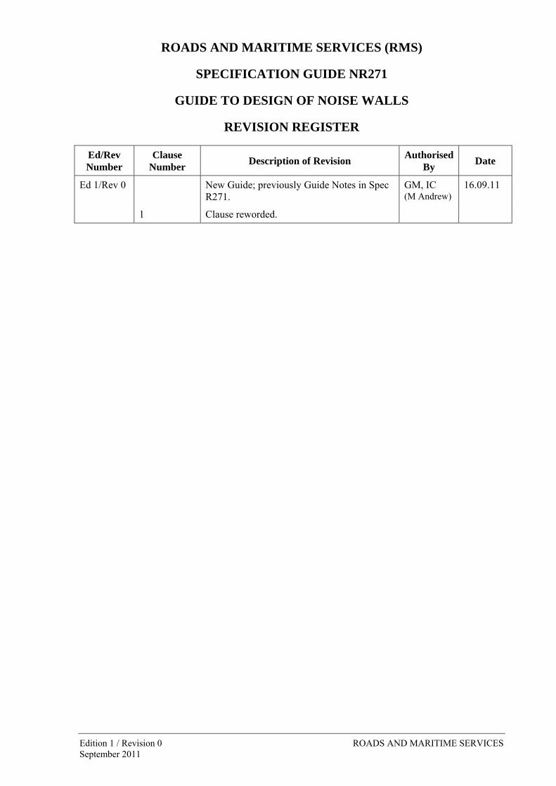
REVISION REGISTER

Ed/Rev Number

Clause Number

Description of Revision Authorised

By Date

Ed 1/Rev 0 New Guide; previously Guide Notes in Spec R271.

GM, IC (M Andrew)

16.09.11

1 Clause reworded.

Edition 1 / Revision 0 ROADS AND MARITIME SERVICES September 2011

Edition 1 / Revision 0 ROADS AND MARITIME SERVICES


GUIDE TO DESIGN OF NOISE WALLS Copyright – Roads and Maritime Services

IC-QA-NR271

VERSION FOR: DATE:

September 2011

Guide to Design of Noise Walls NR271

CONTENTS

CLAUSE PAGE

FOREWORD ...............................................................................................................................................II RMS Copyright and Use of this Document ...................................................................................ii Base Specification..........................................................................................................................ii

1 GENERAL........................................................................................................................................1

2 STRUCTURAL DESIGN ....................................................................................................................1 2.1 Selection of Design Parameters [Specification R271 Clause 3.5.2]...............................1 2.2 Calculation of Wind Loads [Specification R271 Clause 3.5.5]......................................2 2.3 Examples of Wind Load Calculations ..........................................................................17

3 EARTHQUAKE LOADS [Specification R271 Clause 3.5.8]............................................................30 3.1 Design Procedure [Specification R271 Clause 3.5.8(a)] ..............................................30

LAST PAGE OF THIS DOCUMENT IS..........................................................................................................33

Ed 1 / Rev 0 i

NR271 Guide to Design of Noise Walls

ii Ed 1 / Rev 0

FOREWORD

RMS COPYRIGHT AND USE OF THIS DOCUMENT

Copyright in this document belongs to the Roads and Maritime Services.

The Guide is not a contract document. It has been prepared to provide readers with guidance on the use of the specification.

BASE SPECIFICATION

This document is based on RMS QA Specification R271 Edition 2 Revision 0.

(RMS COPYRIGHT AND USE OF THIS DOCUMENT - Refer to the Foreword after the Table of Contents)


GUIDE TO DESIGN OF NOISE WALLS

1 GENERAL

Specification R271 contains several clauses on the design of noise walls for wind and earthquake loads, lateral soil pressures, as well as the design requirements for foundations.

The specification is structured such that most of the design inputs required are listed in Annexure R271/A “Project Specific Requirements” of the Specification. This reduces the discretion of the designer on the choice of the values of the design inputs, in order to minimise errors caused by the misinterpretation of standards and applicable topographic features. This should lead to more consistency in the designs from different tenderers and enable a better comparison of these tenders.

Notwithstanding the above, as permitted under Clause 2.3.1 of Specification R271, more detailed calculations in accordance with AS/NZS 1170.2 and AS 1170.4 can be undertaken where appropriate.

These Guide Notes have been written to facilitate the provision of the design inputs in Annexure R271/A of Specification R271.

As many Australian Standards are constantly under revision, and in some cases, different standards give conflicting requirements, in order to maintain the consistency, the relevant provisions from these standards have been extracted, simplified and consolidated in Specification R271.

As the predominant loading on noise walls is from wind forces and long lengths of noise walls may be required, this design action has been given particular attention.

2 STRUCTURAL DESIGN

2.1 SELECTION OF DESIGN PARAMETERS [Specification R271 Clause 3.5.2]

The first step in the design process is to subdivide the noise walls in the project into representative “Segments”, for which design parameters are common to all walls in the segment.

In accordance with AS/NZS 1170.0, the design working life of a structure (N) is the minimum number of years for which a structure or a structural element must be serviceable for its intended purpose with minimum maintenance without major structural repairs being necessary. AS 5100.2 which is the loading part of the Bridge Design Code specifies certain requirements for noise walls in Clause 24 including a design life of 50 years for these structures.

For each segment the importance level (I) of the noise wall should be assessed in accordance with Table R271.1 of Specification R271. Together with the design life, this determines the annual probability of exceedance of the design event of wind as well as earthquake, and hence its magnitude.

The annual probability of exceedance of a design event for ultimate limit states is specified in Appendix F of AS/NZS 1170.0. The annual probability of exceedance is expressed as a reciprocal (1/R), where R is termed variously as “return period” or “average recurrence interval” or “average return interval” in literature. It expresses the mathematical probability that an event with an average

Ed 1 / Rev 0 1



2 Ed 1 / Rev 0

recurrence interval of R years has a probability of being exceeded in any one year of 1/R. Note that the probability of the event being exceeded during the full design life of a structure (PN) is much higher and is given by:

NN RP 111

(G.1)

For example, the probability that an event with an average recurrence interval of 200 years will be exceeded in any one specified year is 1/200=0.005. If the design life is N = 50 years the probability of exceeding the event at least once during the design life is:

P50 = 1 – [1 – 0.005]50 = 0.222 (G.2)

The annual probabilities of exceedance for ultimate limit state design of structures for wind and earthquake are specified for various importance levels and design life periods in Table F2 of AS/NZS 1170.0.

However, the “average return interval” for noise walls in different situations is also specified in AS 5100.2, Clause 24.2, with some discrepancy between the two standards. In Table R271.1 of Specification R271, this discrepancy is reconciled by increasing some of the R values in AS 5100.2 to match their descriptions with the importance levels defined in AS/NZS 1170.0. Table F2 in AS/NZS 1170.0 is more comprehensive and also includes the earthquake load case, and hence should be followed. As the modifications to AS 5100.2 are on the conservative side, these modifications should be acceptable.

2.2 CALCULATION OF WIND LOADS [Specification R271 Clause 3.5.5]

The wind pressure exerted on a body is dependent on four factors:

(i) The free stream velocity of the wind in the region;

(ii) The shape of the body, which modifies the wind flow pattern around it and hence the aerodynamic drag force;

(iii) The terrain category, which modifies the free stream velocity of the wind within the boundary layer; and

(iv) The topography, which increases the velocity of the wind around large obstructions.

Each factor is considered independently and their product evaluated, even though some interaction exists between them.

In the clauses pertaining to wind loads, “the wind code” refers to AS/NZS 1170.2. The notation in the Specification is consistent with this standard unless specified otherwise in Annexure R271/N of Specification R271.

2.2.1 Wind Tunnel Model Studies

Noise walls are different types of structures from buildings and built in a wide variety of topographic conditions. Considering the difficulties involved in interpreting the recommendations in the 1989 wind code, and the economic and structural implications for the design of noise walls, RMS, in 1999, conducted wind tunnel model tests for walls constructed in different topographic conditions.

Figure NR271.1 shows the types of models that were tested[1]i. Results were compared by calculating the wind pressure on the wall (pc) in accordance with the prevailing code provisions of AS 1170.2:1989 with the pressure measured in the test (pm) after blockage corrections[2] for each case.

i Numbers refer to reports and publications listed in Annexure R271/M3.



It was found that the calculated pressures were over-estimated for certain topographic conditions and under-estimated for others.

H =

16

8

4

43.

2

80H

= 1

6

4

43.

2

Escarpment

Hill

H =

16

4

4

16

80

4016 24

74

(e) Cutting at bottom of hill

(f) Cutting half way up a hill

(g) Cut and fill near bottom of hill

w

(b) Embankment

H

(c) Cliff (d) Bridge

w

(a) On level ground

NOTE: All dimensions are in metres

h

4m T

YP

hH

h

H

s

c

20 40

w

hb

11.31°

32

Models.cad 16/12/2005

15

15

15

16 64

w

Figure NR271.1 - Models Tested in Wind Tunnel

One explanation for the discrepancies between the test results and the values predicted by the then wind code is that the topographic feature and the noise wall interact with each other. In the 1989 wind code, the hill shape multiplier (Mh) and the net pressure coefficient (Cp,n) are treated as independent variables, implying that the structure itself does not influence the wind flow pattern on the topographic feature. This assumption may be valid for a small building on a large hill, for example, but for a noise

Ed 1 / Rev 0 3



wall on an embankment of almost equal height, this condition is not valid. Therefore, some modifications to the equations presented in the 1989 wind code were considered essential.

Note that force based on the net pressure coefficient must always be applied normal to the wall, for structural design, regardless of the actual direction of the wind.

Subsequently, the procedure for computing the topographic multiplier was also modified in the revised wind code, AS/NZS 1170.2:2002. Hence, further analysis of the wind tunnel experimental results was undertaken in 2005[3] based on more precise, statistical principles. The ratio r = pc /pm was calculated for each test and the mean (r) and standard deviation (r) of the values for each set of similar tests were calculated. A value of r close to 1.0 shows good agreement between the calculated and measured values and a low standard deviation indicates that the formula consistently predicts accurate pressures. As it is advisable that the calculated pressure should be slightly higher than the measured value, the following indicator was used:

= r - r (G.3)

Minor modification to the wind code formulas was then attempted to achieve a value of close to 1.0, and a coefficient of variation (= r / r) of approximately 0.1 i.e. 10%. Table C1.4 of AS/NZS 1170.2 commentary shows that most of the design parameters such as VR, M-multipliers, Cfig, etc., have a coefficient of variation of this magnitude or greater. Although the range of parameters tested was albeit limited, it was shown that with the modifications, these assessment criteria were nearly achieved [3], [4].

The modifications to the wind code procedures are outlined in the following sections of these Guide Notes. Application of the modified formulas is clarified with several examples.

2.2.2 Regional Wind Speed [Specification R271 Clause 3.5.5 (a)]

Regional wind speed (VR) is tabulated for regions of New South Wales. For other regions, refer to Figure 3.1 and Table 3.1 of AS/NZS 1170.2.

2.2.3 Terrain/Height Multiplier [Specification R271 Clause 3.5.5 (b)]

The free stream velocity of the wind occurs only at a large height above ground, whereas it is zero when in contact with the ground, and increases gradually with height within the boundary layer. When wind blows over a surface with constant roughness characteristics, the wind profile gradually develops into a constant profile over a considerable distance.

When the surface characteristics change, the velocity profile changes gradually with distance from one category to another. For example, in Figure NR271.2(a), assume that at A the velocity profile is fully developed over the grassland extending a long distance upwind. When the terrain changes at B to a rougher category, the boundary layer extends further up and develops fully at point C, at a distance BC 2500 m.

The height of a fully developed boundary layer is also very large. At smaller heights (z), which are of interest for noise walls, as shown in Figure NR271.2(b), the length of the transition zone (xi) is given by Equation 4.2 in the wind code. For example, in Terrain Category 3, xi = 27 m for z = 3 m; xi = 50 m for z = 5 m; xi = 120 m for z = 10 m; etc.

The significant forces are those acting on the upper portion of the noise wall. Hence, the surface characteristics close to the upstream face are of much less significance. The significant terrain is the one extending from a distance of 10z to 20z upwind of the structure (Clause C4.2.3 of commentary of the wind code). For example, in Figure NR271.2(b), the relevant terrain category to consider is the grassland and not the smooth surface.

4 Ed 1 / Rev 0



(a) Variation in velocity with terrain roughness

A B C

z

20z

Bou

ndar

y la

yer

Transitionzone

Noise barrier

(b) Transition zone upwind of a noise barrier

GrasslandHouse

Velocity

Figure NR271.2 – Development of Boundary Layer

If the surface characteristic changes within the range of 10z to 20z, the smoother of the two surfaces may be considered, conservatively, in lieu of the complex averaging procedure given in the wind code. The terrain near noise walls most probably falls under Category 3 – “Terrain with numerous closely spaced obstructions 3 m to 5 m high such as areas of suburban housing”, because suburbia is where noise walls will be located.

When the noise wall is on the top of a hill or embankment, the velocity within the boundary layer changes due to the slope as well as the roughness and the height of the transition zone cannot be readily calculated. Hence, the smoothest terrain category within a distance of 20z upwind of the noise wall should be considered, conservatively. The value of Mz,cat is still based on the height z.

2.2.4 Evaluation of Topographic Multiplier [Specification R271 Clause 3.5.5 (c)]

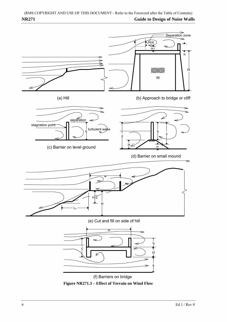
Large features, such as hills, escarpments, cliffs, cuttings and bridges, modify the velocity of the wind blowing over it, as shown by the pattern of stream lines in Figure NR271.3. The velocity increases where the streamlines converge and vice versa.

The noise wall also affects the flow pattern around it, as shown in Figure NR271.3(c). On the upwind side the kinetic energy is converted to pressure in the region below the stagnation point. On the downwind side, an additional drag force acts within the turbulent wake. The net pressure coefficient Cp,n is due to the sum of these two effects, in the proportion 60% to 40% respectively, approximately.

Ed 1 / Rev 0 5



6 Ed 1 / Rev 0

Figure NR271.3 – Effect of Terrain on Wind Flow

fill

(a) Hill (b) Approach to bridge or cliff

H

h

H/2 H

(e) Cut and fill on side of hill

stagnation point turbulent wake

(c) Barrier on level ground

(d) Barrier on small mound

h

separation

c

H

H/

z

Separation zone

H/1

L u

w

w

H

s

c

(f) Barriers on bridge

H/4

h

hb



The topographic multiplier (Mt) is applicable if the noise wall is on a hill, ridge or escarpment and is defined in Clause 4.4.2 of the wind code. However, in Specification R271, Mt is computed as per Clause 2.2.4.3 of these Guide Notes.

If the height of the noise wall is small compared to the height of the topographic feature, as shown in Figure NR271.3(a) and Figure NR271.3(b), the noise wall does not appreciably affect the pattern of stream lines over the hill and application of the hill shape multiplier is straightforward.

In many cases, the height of the noise wall is not negligible compared to the height of the topographic feature and the two elements interact to produce a complex flow pattern, as illustrated in Figure NR271.3(e). Therefore, model testing in a wind tunnel was undertaken for RMS to study the effects of certain common topographic conditions, as shown in Figure NR271.1. Models with a number of different dimension ratios of h/H, w/h and a/c were tested to determine the net pressure coefficients directly. Equations given in the wind code were then slightly modified to obtain the best fit with observed results, as described in Clauses 2.2.1 and 2.2.4.3.

The circular arrows in Figure NR271.3 indicate regions of turbulence and reversed flow. The wind pressure on the noise wall is not constant but fluctuates constantly, due to variation in wind speed, as well as the turbulence in the wake downstream, even when under constant wind velocity. The Cp,n values adopted for design are representative of peak gust wind speeds over a 2 to 3 second interval.

In some cases, the pressure fluctuation is such that the wall is subjected to alternating positive and negative pressures. The positive pressure is generally greater, but, in rare cases, the negative pressure may be greater. This was found in the model tests when parallel noise walls were placed very close together, at spacing equal to the height of the noise wall, but this condition may occur rarely on roadways.

2.2.4.1 Hill Shape Multiplier

The hill shape multiplier is given by Equation 4.4(2) of the wind code, expressed in slightly modified form here:

11

15.3

1nL

x

Lz

HM h (G.4)

where:

H = height of the hill, ridge or escarpment

Lu = horizontal distance upwind from the crest of the hill, ridge or escarpment to a level half the height below the crest

L1 = the greater of 0.36Lu or 0.4H

x = horizontal distance upwind or downwind of the structure to the crest of the hill, ridge or escarpment

n = a factor equal to 4 upwind for all types and downwind for hills and ridges, or 10 downwind for escarpments

z = reference height on the structure above the average local ground level

The hill shape multiplier is applicable within the local topographic zone, for a distance (L2) from the crest given by L2 = nL1 and is also applicable for slopes exceeding 0.05. In other cases Mh = 1.

Within the separation zone (Figure NR271.3(b), the term in square brackets [ ] in Equation G.4 attains its maximum value of 0.71, as per the wind code. However, this should be applied only if the noise wall is fully within the separation zone (h < 0.1H). Such high values of Mh were not

Ed 1 / Rev 0 7



measured in the wind tunnel tests, where noise wall heights varied from 1H to 0.25H. For noise wall heights between 0.1H and 0.25H, values of Mh may be linearly interpolated.

Minor features, such as mounds and small embankments (H < h), may be treated in a simplified manner, without calculating a hill shape multiplier. Comparison of the air flow patterns for Cases (c) and (d) in Figure NR271.3 shows that the height of the turbulent zone is slightly larger in Case (d), for noise walls of the same height. It is proposed that the value of Cp,n based on height h may be factored by z/c to account for this effect.

2.2.4.2 Hill Shape Multiplier Tables

It is not readily apparent how Mh in Equation G.4 varies with the height and slope of the hill and the position of the noise wall on it. Some insight can be gained by modifying Equation G.4 so that it is expressed in dimensionless form in terms of the following two ratios and the average slope of the upper half of the hill tan. They are defined as:

= H/z (G.5a)

= │x│/H (G.5b)

tan = ½H/Lu (G.5c)

Equation G.4 can now be written as:

HnL

Hx

zL

zHM h /

/1

/15.3

/1

11

(G.6)

Substituting for Lu from Equation G.5c in the definition for L1, we have:

L1 = the greater of 0.18H/tan and 0.4H

Hence:

L1 =0.18H/tan for tan< 0.45 (G.7a)

L1 =0.4H for tan 0.45 (G.7b)

Substituting the above values in Equation G.6, we have:

tan/18.0

1tan/18.015.3

1n

M h for tan < 0.45 (G.8a)

n

M h 4.01

4.015.31

for tan 0.45 (G.8b)

A quick estimate of the value of Mh can be made with the help of Table NR271.1 and approximate values can be used in lieu of detailed calculations. Considering the approximations involved in assessing the topographic parameters, undue effort to calculate or interpolate values of Mh to 3 decimal places is not necessary.

8 Ed 1 / Rev 0



Table NR271.1 – Values of Hill Shape Multiplier (Mh)

(a) HILL SHAPE MULTIPLIER (M h) FOR SLOPE tan= 0.05 (1 V : 20 H)L2 = 4L1 L2 = 10L1

= |x|/H = |x|/H = H/z 0 4 8 12 14.4 0 6 12 18 24 36

0 1.00 1.00 1.00 1.00 1.00 1.00 1.00 1.00 1.00 1.00 1.001 1.06 1.04 1.03 1.01 1.00 1.06 1.05 1.04 1.03 1.02 1.002 1.07 1.05 1.03 1.01 1.00 1.07 1.06 1.05 1.03 1.02 1.003 1.07 1.05 1.03 1.01 1.00 1.07 1.06 1.05 1.04 1.02 1.00

4 1.07 1.05 1.03 1.01 1.00 1.07 1.06 1.05 1.04 1.02 1.005 1.08 1.05 1.03 1.01 1.00 1.08 1.06 1.05 1.04 1.03 1.00

10 1.08 1.06 1.03 1.01 1.00 1.08 1.06 1.05 1.04 1.03 1.0015 1.08 1.06 1.03 1.01 1.00 1.08 1.06 1.05 1.04 1.03 1.0020 1.08 1.06 1.03 1.01 1.00 1.08 1.07 1.05 1.04 1.03 1.00

(b) HILL SHAPE MULTIPLIER (M h) FOR SLOPE tan= 0.15 (1 V : 6.66 H)L2 = 4L1 L2 = 10L1

= |x|/H = |x|/H = H/z 0 1 2 4 4.8 0 2 4 6 9 12

0 1.00 1.00 1.00 1.00 1.00 1.00 1.00 1.00 1.00 1.00 1.001 1.13 1.10 1.08 1.02 1.00 1.13 1.11 1.09 1.06 1.03 1.002 1.17 1.13 1.10 1.03 1.00 1.17 1.14 1.11 1.08 1.04 1.003 1.19 1.15 1.11 1.03 1.00 1.19 1.16 1.12 1.09 1.05 1.00

4 1.20 1.16 1.11 1.03 1.00 1.20 1.16 1.13 1.10 1.05 1.005 1.20 1.16 1.12 1.03 1.00 1.20 1.17 1.14 1.10 1.05 1.00

10 1.22 1.17 1.13 1.04 1.00 1.22 1.18 1.15 1.11 1.05 1.0015 1.23 1.18 1.13 1.04 1.00 1.23 1.19 1.15 1.11 1.06 1.0020 1.23 1.18 1.13 1.04 1.00 1.23 1.19 1.15 1.11 1.06 1.00

(c) HILL SHAPE MULTIPLIER (M h) FOR SLOPE tan= 0.25 (1 V : 4 H)L2 = 4L1 L2 = 10L1

= |x|/H = |x|/H = H/z 0 0.5 1 2 2.88 0 1 2 4 6 7.2

0 1.00 1.00 1.00 1.00 1.00 1.00 1.00 1.00 1.00 1.00 1.001 1.17 1.14 1.11 1.05 1.00 1.17 1.14 1.12 1.07 1.03 1.002 1.23 1.19 1.15 1.07 1.00 1.23 1.20 1.17 1.10 1.04 1.003 1.27 1.22 1.18 1.08 1.00 1.27 1.23 1.20 1.12 1.05 1.00

4 1.29 1.24 1.19 1.09 1.00 1.29 1.25 1.21 1.13 1.05 1.005 1.31 1.26 1.20 1.09 1.00 1.31 1.27 1.22 1.14 1.05 1.00

10 1.35 1.29 1.23 1.11 1.00 1.35 1.30 1.25 1.15 1.06 1.0015 1.36 1.30 1.24 1.11 1.00 1.36 1.31 1.26 1.16 1.06 1.0020 1.37 1.31 1.24 1.11 1.00 1.37 1.32 1.27 1.16 1.06 1.00

(d) HILL SHAPE MULTIPLIER (M h) FOR SLOPE tan= 0.35 (1 V : 2.86 H)L2 = 4L1 L2 = 10L1

= |x|/H = |x|/H = H/z 0 0.5 1 1.5 2.06 0 1 2 3 4 5.14

0 1.00 1.00 1.00 1.00 1.00 1.00 1.00 1.00 1.00 1.00 1.001 1.19 1.14 1.10 1.05 1.00 1.19 1.15 1.12 1.08 1.04 1.002 1.28 1.21 1.14 1.08 1.00 1.28 1.23 1.17 1.12 1.06 1.003 1.34 1.26 1.17 1.09 1.00 1.34 1.27 1.21 1.14 1.07 1.00

4 1.37 1.28 1.19 1.10 1.00 1.37 1.30 1.23 1.16 1.08 1.005 1.40 1.30 1.21 1.11 1.00 1.40 1.32 1.24 1.17 1.09 1.00

10 1.47 1.35 1.24 1.13 1.00 1.47 1.37 1.28 1.19 1.10 1.0015 1.49 1.37 1.25 1.13 1.00 1.49 1.40 1.30 1.20 1.11 1.0020 1.51 1.38 1.26 1.14 1.00 1.51 1.41 1.31 1.21 1.11 1.00

(e) HILL SHAPE MULTIPLIER (M h) FOR SLOPE tan= 0.45 (1 V : 2.22 H)L2 = 4L1 L2 = 10L1

= |x|/H = |x|/H = H/z 0 0.4 0.8 1.2 1.6 0 0.5 1 2 3 4

0 1.00 1.00 1.00 1.00 1.00 1.00 1.00 1.00 1.00 1.00 1.001 1.20 1.15 1.10 1.05 1.00 1.20 1.18 1.15 1.10 1.05 1.002 1.32 1.24 1.16 1.08 1.00 1.32 1.28 1.24 1.16 1.08 1.003 1.39 1.29 1.19 1.10 1.00 1.39 1.34 1.29 1.19 1.10 1.00

4 1.44 1.33 1.22 1.11 1.00 1.44 1.38 1.33 1.22 1.11 1.005 1.48 1.36 1.24 1.12 1.00 1.48 1.42 1.36 1.24 1.12 1.00

10 1.57 1.43 1.29 1.14 1.00 1.57 1.50 1.43 1.29 1.14 1.0015 1.61 1.46 1.31 1.15 1.00 1.61 1.54 1.46 1.31 1.15 1.0020 1.63 1.48 1.32 1.16 1.00 1.63 1.56 1.48 1.32 1.16 1.00

Ed 1 / Rev 0 9



In practical situations, the slope of a hill varies with the direction in which the cross section is taken. Equation G.8a and Equation G.8b serve as a useful guide in deciding which is the critical direction to investigate.

(i) If the slope exceeds 0.45, Equation G.8b applies, in which Mh is independent of the slope and therefore attains its maximum value when ξ is minimum. Therefore, the critical direction is always normal to the wall, where x is minimum.

(ii) If the slope is less than 0.45 but is constant along the length, as for an embankment, the critical direction is still normal to the wall. In any other direction, ξ increases and tan reduces. Hence, Mh reduces, as seen from Table NR271.1.

(iii) Where the slope is less than 0.45 but varies with direction, it is recommended to adopt the maximum value of tan within a sector ± 45º normal to the wall.

2.2.4.3 Hill Slope Modifier and Topographic Multiplier

As stated earlier, measured peak pressures on the noise wall models did not correlate very well with values calculated by means of the hill shape multiplier, Equation G.4, especially for complex topographic conditions. An attempt was therefore made to improve the correlations by modifying the wind code formula. The following modification gave much better results (lower values of r):

ht kMM (G.9)

The hill slope modifier (k) is given by:

k = 1 + 0.7 tan – 1.5 (tan for tan 2/3 (i.e. 33.7º) (G.10a)

k= 0.8 for tan > 2/3 (G.10b)

Typical values of k are shown in Table NR271.2.

Table NR271.2 – Hill Slope Modifier

(degrees) 0 10 13 20 25 33 34 to 90 slope (tan 0 0.1763 0.2309 0.3640 0.4663 0.6494 0.67 - ∞ Modifier (k) 1.000 1.077 1.082 1.056 1.000 0.822 0.800

2.2.4.4 Multiplier for Bridges

It is apparent from Figure NR271.3(f) that noise walls on bridges can be analysed as hoardings and Cp,n calculated by means of Equation G.16a below by substituting:

c = hb + H (G.11a)

h = hb + H + s (G.11b)

where:

hb = height of the noise wall, plus edge traffic barrier, if any, above deck level

H = depth of the deck structure

s = clear height under the deck

Also, for assessing Mz,cat, adopt z = h.

Some consideration is required regarding the position of the noise wall on the bridge and whether there are noise walls on both sides or only on one side.

10 Ed 1 / Rev 0



Ed 1 / Rev 0 11

For the noise wall on the upwind side, the value of Cp,n calculated as above agrees well with the results of the model tests. It is immaterial whether there is another noise wall on the other side of the deck or not.

If there are noise walls on both sides, the downwind side noise wall is subjected to shielding from the upwind side noise wall and may even experience reverse flow, as seen from Figure NR271.3(f). However, as it also has to be designed as an upwind noise wall for wind acting in the opposite direction, this condition would most probably govern the design.

If there is a noise wall on one side of the bridge only, for the downwind noise wall, which is away from the leading edge of the deck, it is reasonable to expect that an effect similar to an escarpment will occur. Correlation with model test values was improved by applying the following multiplier:

Hs

xM b

15

1 (G.12)

where:

x = distance of noise wall from upwind edge of bridge

The topographic multiplier (Mt) can be replaced by Mb in case of bridges. For the upwind noise wall, we have x = 0, and hence Mb = 1. For a noise wall on one side only, in the downwind direction Equation G.12 is applicable with x = width of bridge deck.

2.2.4.5 Shielding Multiplier

Shielding of one wall by another has the effect of reducing the wind pressure on the downwind wall. Any change in environmental or structural conditions, such as widening of the roadway in future, can eliminate shielding. For design of new walls, no reduction in pressure due to shielding is allowed (Ms = 1) in accordance with AS 5100.2. In case it is necessary to check the safety of a wall in an existing situation, shielding may be considered.

For the models tested, the following multiplier (Ms) was found to give satisfactory predictions

of the pressure on downwind walls on level ground, for h

w> 4.5:

2

51

w

hM s 0.75 Ms 1.0 (G.13)

where:

w = spacing between parallel walls

h = height of panel

When parallel walls are placed close together (at spacing less than 4 times the height of the walls), shielding causes recirculation of flow behind the upwind wall, and hence a negative pressure on the downwind wall; see Figure NR271.3(e) and Figure NR271.3(f). Therefore, even if this wall is completely shielded from wind in the other direction, ensure its stability in both directions.

2.2.4.6 Other Topographic Conditions

The conditions illustrated in Cases (e), (f) and (g) of Figure NR271.1 were tested by means of models in the wind tunnel. Reasonable correlations were obtained between the calculated and measured peak pressures; however, it must be understood that there is a practical limit to the number of cases that could be tested. Table NR271.3 shows the range of variables tested. If the



actual parameters are not within these limits, it is recommended that reduction factors proposed here not be applied and the wind code provisions interpreted conservatively, based on concepts outlined in Clauses 2.2.3 and 2.2.4.

Table NR271.3 – Range of Variables Tested by Models

Model type Case in

Figure G.1 h

w

H

h

c

a Other

limitations

On level ground a 1 to 7 1 to 4

On embankments b 1 to 7 0.25 to 1 1 to 4 tan = 2/3

On cliffs c 1 to 7 0.25 to 1 1 to 4

On bridges d 4 1 1 to 4 s/H = 2 to 4

Cutting at bottom of hill e 4 0.25 1 to 4 tan = 0.2 x > L2

Cutting half way up hill f 4 0.25 1 to 4 tan = 0.2

Cut and fill g 4 0.25 1 to 4 tan = 0.2

2.2.5 Calculation of Design Wind Velocity [Specification R271 Clause 3.5.5(a)]

The site wind speed in a direction whose bearing is is calculated as per Clause 2.2 of the wind code by:

Vsit, = VR Md (Mz,cat Ms Mt) (G.14)

The pressure on the wall also depends on the pressure coefficient (Cp,n) and is defined in Clause D2 of the wind code for 3 different values of , the angle of wind to the normal to the wall. As wind acting in any direction has to be catered for, strictly, 8 different wind directions in increments of 45° have to be considered. However, the following simplifications enable considerable reduction in the calculations.

(i) The risk of the wall toppling on one side or the other can be assessed and, accordingly, VR can have at most two values, one for each side of the wall.

(ii) The terrain may be classified into at most two different categories, one on each side of the wall.

(iii) For the design of new walls, shielding is not to be considered. Hence, only in exceptional cases will Ms have a value other than 1.0.

(iv) Evaluation of the topographic multiplier (Mt) has been discussed in Clause 2.2.4. As this calculation is based on empirical formulas, even if the topography varies with direction, elaborate calculations for Mt in several different directions may not be worthwhile. A reasonable approximation is to base the evaluation of Mt on the maximum slope on each side of the wall. For cuttings or embankments, the cross section normal to the wall would be considered for calculating Mt.

With the above simplifications, VR, Mz,cat Ms and Mt are constant for each side of the wall. The value of Vsit, is then proportional to Md on each side. Further, as Ms = 1, the simplified design equation is:

Vdes = VR Md Mt Mz,cat (G.15)

The effect of variation in Cp,n is discussed in Clause 2.2.6.2. Accordingly, there are two options:

12 Ed 1 / Rev 0



Ed 1 / Rev 0 13

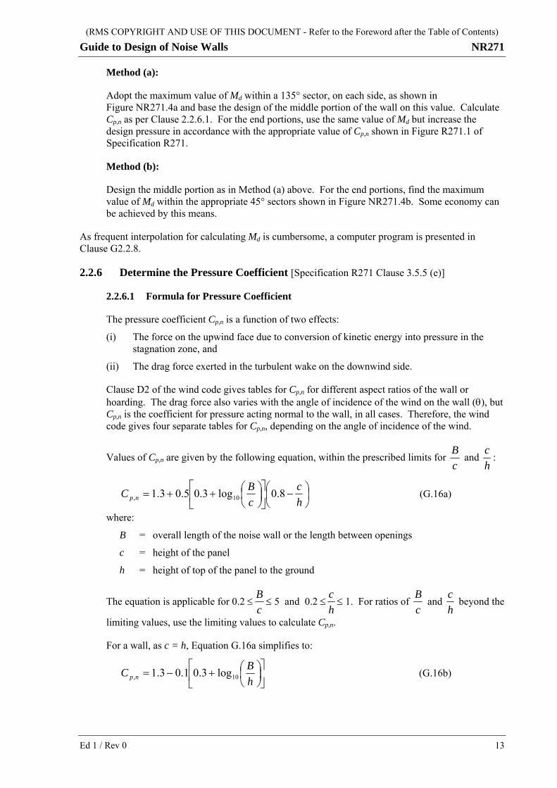
Method (a):

Adopt the maximum value of Md within a 135° sector, on each side, as shown in Figure NR271.4a and base the design of the middle portion of the wall on this value. Calculate Cp,n as per Clause 2.2.6.1. For the end portions, use the same value of Md but increase the design pressure in accordance with the appropriate value of Cp,n shown in Figure R271.1 of Specification R271.

Method (b):

Design the middle portion as in Method (a) above. For the end portions, find the maximum value of Md within the appropriate 45° sectors shown in Figure NR271.4b. Some economy can be achieved by this means.

As frequent interpolation for calculating Md is cumbersome, a computer program is presented in Clause G2.2.8.

2.2.6 Determine the Pressure Coefficient [Specification R271 Clause 3.5.5 (e)]

2.2.6.1 Formula for Pressure Coefficient

The pressure coefficient Cp,n is a function of two effects:

(i) The force on the upwind face due to conversion of kinetic energy into pressure in the stagnation zone, and

(ii) The drag force exerted in the turbulent wake on the downwind side.

Clause D2 of the wind code gives tables for Cp,n for different aspect ratios of the wall or hoarding. The drag force also varies with the angle of incidence of the wind on the wall (), but Cp,n is the coefficient for pressure acting normal to the wall, in all cases. Therefore, the wind code gives four separate tables for Cp,n, depending on the angle of incidence of the wind.

Values of Cp,n are given by the following equation, within the prescribed limits for c

B and

h

c:

h

c

c

BC np 8.0log3.05.03.1 10, (G.16a)

where:

B = overall length of the noise wall or the length between openings

c = height of the panel

h = height of top of the panel to the ground

The equation is applicable for 0.2 c

B 5 and 0.2

h

c 1. For ratios of

c

B and

h

c beyond t

limiting values, use the limiting values to calculate Cp,n.

he

For a wall, as c = h, Equation G.16a simplifies to:

h

BC np 10, log3.01.03.1 (G.16b)



14 Ed 1 / Rev 0

2.2.6.2 Variation with Angle of Incidence of Wind

To comply with Clause D2 of the wind code, the pressure coefficient (Cp,n) has to be calculated for wind acting in several different directions on the wall, in accordance with Tables D2(A) to D2(D). Some simplification can be achieved, as follows.

In Table NR271.4, values of Cp,n have been worked out for different aspect ratios, height ratios and angles of incidence of the wind, which are specified in Tables D2(A) to D2(C) of the wind code. It can readily be seen that values in the shaded portions of Tables G.4(a) and G.4(b) are

the same; values differ only for c

B> 5. As both = 0 and = 45° have to be considered for

design, an envelope of values has been presented in Table G.4(c). An abbreviated version of this table has also been presented in Table R271.3 of Specification R271, accompanied by Figure R271.1.

According to Clause 2.3 of the wind code, the value of Vsit, must be the maximum value within a sector ±22.5° from the nominal direction of the wind. Therefore, if an envelope of Cp,n values for = 0 and = ± 45° is considered, the maximum value of Vsit, within = ± 62.5° to the normal i.e. a 135° sector on each side of the wall must be adopted, as shown in Figure NR271.4b for the examples.

The only difference in Tables NR271.4(a) and NR271.4(b) is in the end portions of the walls (B/c > 5). The pressure coefficient increases significantly towards the free ends for wind acting at 45°. Therefore, for the end portions, economy can be achieved by considering wind only in the relevant sector from - 22.5° to + 22.5° for calculating Vsit, as shown in Figure NR271.4b for example.

The increase in value of Cp,n for wind acting at 45° to the wall is due to unsymmetrical wind flow pattern, which causes higher drag forces on one side of the panel than the other. For isolated panels of length b, the force must be applied at an eccentricity of 0.2b, as specified in Table D2(B) of the wind code. For long noise walls, either continuous or comprising several panels end to end, it is more appropriate to account for this aerodynamic effect by increasing the pressure on the end portions, as specified in Table D2(C) of the wind code.

For wind blowing parallel to a wall, a frictional force will act on the exposed surfaces, depending on the roughness texture of the wall. Additional drag forces will also act on the legs of hoardings. Clause 3.5.5(h) of Specification R271 gives requirements for calculating both these forces. Note that, even for wind blowing parallel to a wall, a normal pressure coefficient has to be considered in accordance with Table D2(D) of the wind code, but its value is much less than for wind at = 0 and = 45°.



Table NR271.4 – Envelope of Values of Pressure Coefficients (Cp,n)

WIND LOADS ON NOISE BARRIERSPRESSURE COEFFICIENTS FOR WALLS/HOARDINGS AS/NZS 1170.2:2002, Clause D2

B = Length of barrier between free ends h = Height of hoardingx = Distance from windward free end c= Height of barrierb = Length of individual panel

Values in shaded cells given by: Cpn = 1.3 + 0.5*[0.3+LOG10(B/c)]*(0.8-c/h)

(a) WIND NORMAL TO WALL = 0 Table D2(A) of AS/NZS 1170.2HEIGHT ASPECT RATIO (B/c)RATIO (c/h) 0.2 0.5 1 2 3 4 5 all x

0.1 1.18 1.30 1.39 1.48 1.53 1.57 1.60 1.60 1.60 1.600.2 1.18 1.30 1.39 1.48 1.53 1.57 1.60 1.60 1.60 1.600.3 1.20 1.30 1.38 1.45 1.49 1.53 1.55 1.55 1.55 1.550.4 1.22 1.30 1.36 1.42 1.46 1.48 1.50 1.50 1.50 1.500.5 1.24 1.30 1.35 1.39 1.42 1.44 1.45 1.45 1.45 1.450.6 1.26 1.30 1.33 1.36 1.38 1.39 1.40 1.40 1.40 1.400.7 1.28 1.30 1.32 1.33 1.34 1.35 1.35 1.35 1.35 1.350.8 1.30 1.30 1.30 1.30 1.30 1.30 1.30 1.30 1.30 1.300.9 1.32 1.30 1.29 1.27 1.26 1.25 1.25 1.25 1.25 1.251 1.34 1.30 1.27 1.24 1.22 1.21 1.20 1.20 1.20 1.20

e = 0.00 0.00 0.00 0.00 0.00 0.00 0.00

(b) WIND at 45 degrees TO WALL = 45° Tables D2(B), D2(C) & D2(D)HEIGHT ASPECT RATIO (B/c)

RATIO (c/h) 0.2 0.5 1 2 3 4 5 x ≤ 2c 2c<x<4c x ≥ 4c0.1 1.18 1.30 1.39 1.48 1.53 1.57 1.60 3.00 1.50 0.750.2 1.18 1.30 1.39 1.48 1.53 1.57 1.60 3.00 1.50 0.750.3 1.20 1.30 1.38 1.45 1.49 1.53 1.55 3.00 1.50 0.750.4 1.22 1.30 1.36 1.42 1.46 1.48 1.50 3.00 1.50 0.750.5 1.24 1.30 1.35 1.39 1.42 1.44 1.45 3.00 1.50 0.750.6 1.26 1.30 1.33 1.36 1.38 1.39 1.40 3.00 1.50 0.750.7 1.28 1.30 1.32 1.33 1.34 1.35 1.35 3.00 1.50 0.75

0.8 1.30 1.30 1.30 1.30 1.30 1.30 1.30 2.40 1.20 0.600.9 1.32 1.30 1.29 1.27 1.26 1.25 1.25 2.40 1.20 0.601 1.34 1.30 1.27 1.24 1.22 1.21 1.20 2.40 1.20 0.60

e = 0.2b 0.2b 0.2b 0.2b 0.2b 0.2b 0.2b x ≤ 2h 2h<x<4h x ≥ 4h

(c) ENVELOPE OF ABOVEHEIGHT ASPECT RATIO (B/c)

RATIO (c/h) 0.2 0.5 1 2 3 4 5 x ≤ 2c 2c<x<4c x ≥ 4c0.1 1.18 1.30 1.39 1.48 1.53 1.57 1.60 3.00 1.60 1.600.2 1.18 1.30 1.39 1.48 1.53 1.57 1.60 3.00 1.60 1.600.3 1.20 1.30 1.38 1.45 1.49 1.53 1.55 3.00 1.55 1.550.4 1.22 1.30 1.36 1.42 1.46 1.48 1.50 3.00 1.50 1.500.5 1.24 1.30 1.35 1.39 1.42 1.44 1.45 3.00 1.50 1.450.6 1.26 1.30 1.33 1.36 1.38 1.39 1.40 3.00 1.50 1.400.7 1.28 1.30 1.32 1.33 1.34 1.35 1.35 3.00 1.50 1.35

0.8 1.30 1.30 1.30 1.30 1.30 1.30 1.30 2.40 1.30 1.300.9 1.32 1.30 1.29 1.27 1.26 1.25 1.25 2.40 1.25 1.251 1.34 1.30 1.27 1.24 1.22 1.21 1.20 2.40 1.20 1.20

e = 0.2b 0.2b 0.2b 0.2b 0.2b 0.2b 0.2b x ≤ 2h 2h<x<4h x ≥ 4h

B/c > 5

B/c > 5

B/c > 5

Ed 1 / Rev 0 15



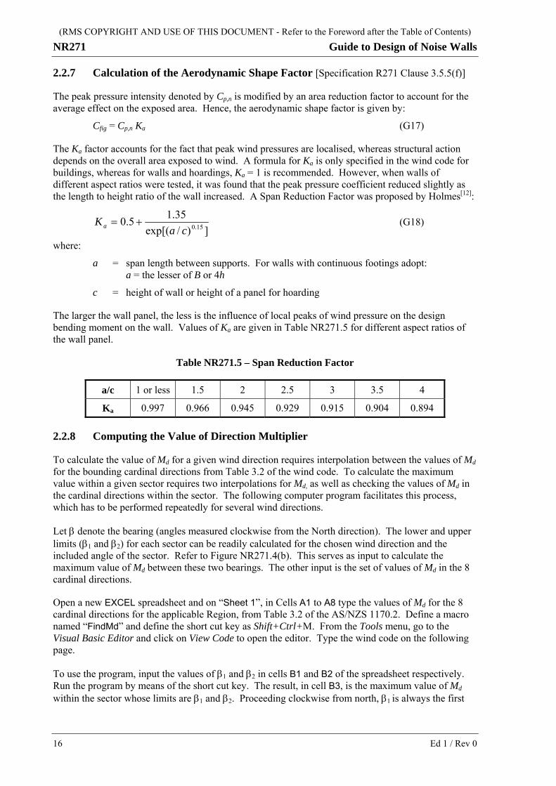
2.2.7 Calculation of the Aerodynamic Shape Factor [Specification R271 Clause 3.5.5(f)]

The peak pressure intensity denoted by Cp,n is modified by an area reduction factor to account for the average effect on the exposed area. Hence, the aerodynamic shape factor is given by:

Cfig = Cp,n Ka (G17)

The Ka factor accounts for the fact that peak wind pressures are localised, whereas structural action depends on the overall area exposed to wind. A formula for Ka is only specified in the wind code for buildings, whereas for walls and hoardings, Ka = 1 is recommended. However, when walls of different aspect ratios were tested, it was found that the peak pressure coefficient reduced slightly as the length to height ratio of the wall increased. A Span Reduction Factor was proposed by Holmes[12]:

])/exp[(

35.15.0

15.0caK a (G18)

where:

a = span length between supports. For walls with continuous footings adopt: a = the lesser of B or 4h

c = height of wall or height of a panel for hoarding

The larger the wall panel, the less is the influence of local peaks of wind pressure on the design bending moment on the wall. Values of Ka are given in Table NR271.5 for different aspect ratios of the wall panel.

Table NR271.5 – Span Reduction Factor

a/c 1 or less 1.5 2 2.5 3 3.5 4

Ka 0.997 0.966 0.945 0.929 0.915 0.904 0.894

2.2.8 Computing the Value of Direction Multiplier

To calculate the value of Md for a given wind direction requires interpolation between the values of Md for the bounding cardinal directions from Table 3.2 of the wind code. To calculate the maximum value within a given sector requires two interpolations for Md, as well as checking the values of Md in the cardinal directions within the sector. The following computer program facilitates this process, which has to be performed repeatedly for several wind directions.

Let denote the bearing (angles measured clockwise from the North direction). The lower and upper limits (1 and 2) for each sector can be readily calculated for the chosen wind direction and the included angle of the sector. Refer to Figure NR271.4(b). This serves as input to calculate the maximum value of Md between these two bearings. The other input is the set of values of Md in the 8 cardinal directions.

Open a new EXCEL spreadsheet and on “Sheet 1”, in Cells A1 to A8 type the values of Md for the 8 cardinal directions for the applicable Region, from Table 3.2 of the AS/NZS 1170.2. Define a macro named “FindMd” and define the short cut key as Shift+Ctrl+M. From the Tools menu, go to the Visual Basic Editor and click on View Code to open the editor. Type the wind code on the following page.

To use the program, input the values of 1 and 2 in cells B1 and B2 of the spreadsheet respectively. Run the program by means of the short cut key. The result, in cell B3, is the maximum value of Md within the sector whose limits are 1 and 2. Proceeding clockwise from north, 1 is always the first

16 Ed 1 / Rev 0



bearing and 2 the second. The maximum value of Md is calculated in the sector going clockwise from 1 to 2.

The program can also be used to interpolate values of Vsit, in accordance with the more detailed analysis outlined in Clause 3.5.6 of Specification R271, by replacing the values of Md by the values of Vsit,. Sub FindMd() ' FindMd Macro ' Macro recorded 27/7/2006 by BhavnagV ' ' Keyboard Shortcut: Ctrl+Shift+M ' J = direction counter ' A(J)= Value of Md in direction J ' B1 and B2 are bearing limits ' C*J is the bearing at J. C=45 degrees. Dim A(16) Dim J As Integer C = 45 ' Get values in cardinal directions from cells A1 to A8 For J = 1 To 8 A(J) = Worksheets("Sheet1").Cells(J, 1) A(J + 8) = A(J) Next J ' Get bearing range from cells B1 and B2 B1 = Worksheets("Sheet1").Cells(1, 2) B2 = Worksheets("Sheet1").Cells(2, 2) ' Locate the initial direction number for B1 For J = 1 To 8 If C * (J - 1) <= B1 And C * J > B1 Then j1 = J End If Next J ' Interpolate Md at B1 M1 = Interpolate(j1, B1, A) ' Locate the initial direction number for B2 For J = 1 To 8 If C * (J - 1) <= B2 And C * J > B2 Then j2 = J End If Next J

M2 = Interpolate(j2, B2, A)

' Find maximum interpolated value Md = M1 If M2 > M1 Then Md = M2 End If ' Check cardinal values from B1 to B2 If j2 < j1 Then j3 = j2 + 8 Else j3 = j2 End If For J = j1 + 1 To j3 If A(J) > Md Then Md = A(J) End If Next J Worksheets("Sheet1").Cells(3, 2) = Md ' Result (Max Md) is in cell B3 of Sheet 1 End Sub Function Interpolate(ByVal J, ByVal X, ByRef A) As Single C = 45 X1 = C * (J - 1) X2 = C * J If X1 = X2 Then Interpolate = Y1 Else Y1 = A(J) Y2 = A(J + 1) Interpolate = Y1 + (Y2 - Y1) / (X2 - X1) * (X - X1) End If

End Function

2.3 EXAMPLES OF WIND LOAD CALCULATIONS

Several examples are presented to illustrate the application of the above design methodology for noise walls that are assumed to be located in different topographic conditions.

Ed 1 / Rev 0 17



2.3.1 General Data for Examples

(i) The walls are in Region A2 of NSW;

(ii) The relevant Terrain Category is 3 unless stated otherwise;

(iii) The design life is N = 50 years;

(iv) The bearing of the wall is 50 degrees.

Direction Multipliers

Figure NR271.4a shows the values of Md entered from Table 3.2 of the wind code for Region A2 for the 8 cardinal directions. The nominal wind directions to be considered are South-east and North-west. The method in Clause 2.2.5 will be followed.

In accordance with Method (a) of Clause 2.2.5, the maximum value of Md within a 135º sector on each side of the wall must be calculated. If the program is used, for the NW direction, the bearing limits are:

1 = 50 + 180 + 22.5 = 252.5 and 2 = 50 – 22.5 = 27.5

Input these and run the program to get Md = 1.0. Note that the sector analysed is in the clockwise direction from 1 to 2. If values of 1 and 2 are interchanged, the maximum value of Md on the SE side over the obtuse angled sector will be calculated.

Figure NR271.4b gives inputs of 1 and 2 and the resulting values of Md for all the relevant sectors that are required to comply with analysis in accordance with Method (b) of Clause 2.2.5.

WALL

N

S

NE

E

SESW

W

NW0.8

0.95

0.9

0.8

0.95

1.0

0.95

= 0.8Md

=252.5º1

=297.5º2

=162.5º1 =207.5º2

M = 0.931d

=27.5º2

=72.5º1

=252.5º1

=207.5º2M = 1.0d

M = 1.0d

M = 0.95d

=342.5º1 =27.5º2

M = 0.858d

=72.5º1

=117.5º2

M = 0.892d

50°

(a) Direction multipliers for cardinal wind directions

N

(b) Direction multipliers calculated for design wind directions on wall

22.5

°

22.5°

22.5°

Figure NR271.4 - Wind Direction Multipliers for Different Sectors

2.3.2 Example 1: Approach to a Bridge

A noise wall is constructed on an approach to a bridge, as shown in Figure NR271.5. The approach is on an embankment sloped at 1:2 on the NW side and retained by a wall on the SE side. The noise wall is a continuous reinforced concrete wall 2.4 m high.

18 Ed 1 / Rev 0



7.3

m

19.0 m

NW SE

1.0 m

3.65

m

7.3 m

uL

2.4 m

12

Figure NR271.5 – Example 1

In accordance with Figure R271.1 of Specification R271 the pressure coefficient (Cp,n) is 1.2 for the middle portion of the wall but increases to 2.4 for end portions 4.8 m long on each side.

For a wall with continuous footings, adopt a = 4h, hence Ka = 0.894 from Table NR271.5.

North-West Wind

Assume that the area at the base of the retaining wall is classified with an importance level I = 4.

From Table R271.1 of Specification R271, we have R = 2500 years.

As per Table R271.2 of Specification R271, the regional wind speed is VR = 48 m/s

Height z = 2.4 m, hence Mz,cat = 0.83.

The embankment forms an escarpment, with:

H = 7.3 m, Lu = 7.3 m, ½H/Lu = tan = 0.5

The scaled lengths are:

L1 = max (0.36Lu, 0.4H) = max (2.628, 2.92) = 2.92 m

L2 = 10L1 = 29.2 m

The noise wall is at x = 19 m from the reference point. The slope exceeds 0.45, but the noise wall is not within the separation zone. It is within the local topographic zone and the hill shape multiplier is given by Equation G.4:

A quick check from Table NR271.1(e) shows that for = H/z = 3.04 and = x/H = 2.6, we have Mh ≈ 1.14.

It was shown in Clause 2.2.4.2 that the critical dimensions for calculating Mh are those normal to the embankment. This can be readily verified here. For wind blowing at an angle of 45º to the wall, the dimension ratios in cross-section are:

= H/z = 3.04, = 1.41 × 2.6 = 3.66 and tan = 0.5/1.41 = 0.355.

Ed 1 / Rev 0 19



From Equation G.8a, we get Mh = 1.095 < 1.14. Hence, this direction is not critical for calculating Mh.

For an embankment, we have, by Equation G.10a,

k = 1 + 0.7 tan - 1.5(tan = 1 + 0.7 × 0.5 – 1.5 × 0.25 = 0.975

The topographic multiplier is therefore:

Mt = 0.975 × 1.137 = 1.11

The design wind speed is:

Vdes = VR Mz,cat Md Mt = 48 × 0.83 × 1.0 × 1.11 = 44.2 m/s

The pressure is:

p = 0.0006 Cp,n Ka Vdes2 = 0.0006 × 1.2 × 0.894 × (44.2)2 = 1.26 kPa

South-East Wind

The noise wall does not cause a serious obstruction to the roadway even if it topples, due to its low height compared to the road width. Hence, adopt I = 3.

From Table R271.1 of Specification R271 we have R = 1000 years, hence VR = 46 m/s.

Height z = 2.4 m, hence Mz,cat = 0.83.

Relevant dimensions for the hill shape multiplier are:

x = 1.0 m, Lu = 0, L1 = 0.4H = 2.92 m, L2 = 4L1 = 11.68 m

Hence:

36.1914.0392.0168.11

11

92.24.25.3

3.71

hM

The height of the separation zone is H/10 = 0.73 whereas the height of the noise wall is 2.4 m. For a ratio of h/H = 2.4/7.3 = 0.328, it is recommended in Clause 2.2.4.1 that no increase be made for this effect.

The proposed modification factor for cliffs is k = 0.8. The topographic multiplier is therefore:

Mt = 0.8 × 1.36= 1.09

The design wind velocity and pressure are, respectively:


p = 0.0006 Cp,n Ka Vdes2 = 0.0006 × 1.2 × 0.894 × (40.6)2 = 1.06 kPa

End Portions

For the end portions, Cp,n increases from 1.2 to 2.4 in accordance with Figure R271.1(a) of Specification R271. If the method in Clause 2.2.5 is followed, Vdes is the same as above. Hence, the design pressure is doubled for a length of 4.8 m at each end in each direction.

20 Ed 1 / Rev 0



However, on the north side, it is seen from Figure NR271.4b that Md is reduced from 1.0 to 0.858. Hence


p = 0.0006 Cp,n Ka Vdes2 = 0.0006 × 2.4 × 0.894 × (37.9)2 = 1.85 kPa < 2 × 1.26 =

2.52 kPa

More Detailed Analysis

Compare results by doing a detailed analysis in accordance with Clause 3.5.6 of Specification R271.

The values of Vsit, have to be calculated for the 8 cardinal directions according to Equation 2.2 of AS/NZS 1170.2. Input the appropriate values of VR and the M-multipliers on each side of the wall and calculate the product, Vsit,, as shown in Table NR271.6.

Table NR271.6 – Calculation of Site Velocity for Example 6

Direction Bearing VR Md Mz,cat Mt Vsit,

N 0 48 0.80 0.83 1.11 35.4

NE 45 48 0.80 0.83 1.11 35.4

E 90 46 0.80 0.83 1.09 33.3

SE 135 46 0.95 0.83 1.09 39.5

S 180 46 0.90 0.83 1.09 37.5

SW 225 46 0.95 0.83 1.09 39.5

W 270 48 1.00 0.83 1.11 44.2

NW 315 48 0.95 0.83 1.11 42.0

For NW wind, the maximum velocity is required between bearings of 252.5° and 27.5° (refer to Figure NR271.6b). This gives Vdes = 44.2 m/s by inspection.

For SE wind, the maximum velocity is required between bearings of 72.5° and 207.5°. This gives Vdes = 39.5 m/s by inspection.

At the NE end, the maximum velocity is required between bearings of 342.5° and 27.5° in the clockwise direction. This gives Vdes = 37.9 m/s after interpolation.

The program in Clause 2.2.8 can be used if values of Md are replaced by those of Vsit,.

The calculated values of Vdes above are the same as those calculated earlier by the simplified method. The more detailed method is required only if Mz,cat or Mt is not constant within a 135° sector.

2.3.3 Example 2: Single Noise Wall on Bridge

A bridge crosses a freeway, as shown in Figure NR271.6. A noise wall is provided only on the SE side, where the Terrain Category is 3. Each wall panel is 2.4 m high and 4.8 m long and is mounted over a traffic barrier approximately 800 mm high. The length of the noise wall is 130 m.

Ed 1 / Rev 0 21



2.40

m2.

00 m

12.0

0 m

0.80 m

16.00 m

SENW


For a bridge structure, the topographic multiplier is 1.0. The height z for Mz,cat is measured from the free surface below; hence, z = 17.2 m.

The noise wall acts as a hoarding with:

B = 130 m, c = 5.2 m, h = 17.2 m

We have B/c = 25 and c/h = 0.3023. To calculate Cp,n , use B/c = 5 for ratios exceeding 5. Therefore, the pressure coefficient for the middle portion is:

Cp,n = 1.3 – 0.1{0.3 + log10(5)} = 1.55

The span reduction factor for one panel is:

Ka = 0.5 + 1.35 / exp[(4.8/2.4)0.15] = 0.945

North-West Wind

A noise wall falling on the freeway below may substantially hinder emergency relief operations; hence, the importance level is I = 4.

We therefore have R = 2500 years and the regional wind speed VR = 48 m/s.

The freeway is classified as Terrain Category 2. Conservatively the values for Mz,2 may be adopted, but, if the terrain changes after some distance, the lag distance may be calculated in accordance with Equation 4.2 of AS/NZS 1170.2:

22 Ed 1 / Rev 0



25.1

,0,0 3.0

rri z

zzx = 420

02.03.0

2.1702.0

25.1

m

Assuming that the freeway runs straight for at least this length, or simply adopting the multiplier for terrain category 2 conservatively, we have, from Table 4.1(A) of AS/NZS 1170.2:

Mz,cat = M17.2, 2 = 1.063

For a single noise wall on the downwind side of the bridge, Equation G.12 gives:

924.021215

161

bM

The design wind speed and pressure for the middle portion are, respectively:

Vdes = VR Mz,cat Md Mb = 48 × 1.063 × 1.0 × 0.924 = 47.1 m/s

p = 0.0006 Cp,n Ka Vdes2 = 0.0006 × 1.55 × 0.945 × (47.1)2 = 1.95 kPa

South-East Wind

Even a partial obstruction of the bridge carriageway by a fallen noise wall may not be considered acceptable; hence:

I = 4, R = 2500 years, VR = 48 m/s.

For Terrain Category 3 at 17.2 m height, interpolating from Table 4.1(A) of AS/NZS 1170.2:

Mz,cat = M17.2, 3 = 0.912

The bridge multiplier Mb = 1 for x = 0.

The design wind speed and pressure for the middle portion are, respectively:

Vdes = VR Mz,cat Md = 48 × 0.912 × 0.95 = 41.6 m/s

p = 0.0006 Cp,n Ka Vdes2 = 0.0006 × 1.55 × 0.945 × (41.6)2 = 1.52 kPa

Structural Design

For the panels at each end, the pressure coefficients must be increased in accordance with Figure R271.1(b) of Specification R271. We have c < 0.7h and 2c = 10.4 m. As panels are 4.8 m long, 3 panels at each end must be designed for Cp,n = 3.0. However, at the North end, Md values can be reduced from 1.0 to 0.858 on the NW side, as shown in Figure NR271.4b. This gives:

Vdes = VR Mz,cat Md Mb = 48 × 1.063 × 0.858 × 0.924 = 40.5 m/s

p = 0.0006 Cp,n Ka Vdes2 = 0.0006 × 1.55 × 0.945 × (40.5)2 = 1.44 kPa

Pressures on the other three end portions can be similarly calculated.

Connections must be designed for a life of 100 years according to Clause 2.2.1 of Specification R271. However, for I = 4, no value for R is specified in Table F2 of AS/NZS 1170.0. R = 2500 years may be accepted as a reasonable upper limit and the same design pressure adopted.

Ed 1 / Rev 0 23



For checking serviceability, adopt R = 20 years according to Clause 3.5.2. Hence VR = 37 m/s from Table R271.2 of Specification R271. The design pressures must therefore be factored by (37/48)2 = 0.594.

2.3.4 Example 3: Road Cut into Side of Hill

This example shows the comparison between pressures calculated for a complex topographical situation with those obtained in the wind tunnel tests. Consider the example in Figure NR271.7, which comprises Case (f) of the model study (Figure NR271.1). For equivalence with the model tests, adopt:

VR = 50 m/s, Md = 1, a/c = 2 and Cp,n = 1.2.

H =

16

m

8 m

h=4

m

4 m

3.2

m

80 m

40 m

16 m 24 m

Guide Ex3.cad 13/12/2005


For a/c = 2 we have Ka = 0.945 from Table NR271.5.

L1 = max (0.36 × 40, 0.4 × 8) = 14.4 m, L2 = 4L1 = 57.6 m

Noise walls on both sides of the road are in the local topographic zone.

k = 1 + 0.7 tan - 1.5(tan = 1 + 0.7 × 0.2 – 1.5 × 0.04 = 1.08

Wind Left to Right; Left Hand Side Noise Wall

The noise wall is at x = – 40 m from the crest of the hill. The hill shape multiplier is:

076.16.57

401

4.1445.3

161

hM

The topographic multiplier, design wind speed and pressure are, respectively:

Mt = k Mh = 1.08 × 1.076 = 1.162

Vdes = VR Mz,cat Md Mt = 50 × 0.83 × 1 × 1.162 = 48.2 m/s

p = 0.0006 Cp,n Ka Vdes2 = 0.0006 × 1.2 × 0.945 × (48.2)2 = 1.58 kPa

The value obtained from the wind tunnel measurement was 1.31 kPa.

Wind Left to Right; Right Hand Side Noise Wall

The noise wall is at x = – 24 m from the crest. Here z = 7.2 m. The hill shape multiplier is:

24 Ed 1 / Rev 0



123.16.57

241

4.142.75.3

161

hM

The topographic multiplier, design wind speed and pressure are, respectively:

Mt = k Mh = 1.08 × 1.123 = 1.213

Vdes = VR Mz,cat Md Mt = 50 × 0.83 × 1 × 1.213 = 50.3 m/s

p = 0.0006 Cp,n Ka Vdes2 = 0.0006 × 1.2 × 0.945 × (50.3)2 = 1.72 kPa

The value obtained from the wind tunnel measurement was 1.61 kPa.

The design pressures are therefore about 10% more conservative than the measured values.

2.3.5 Example 4: Noise Wall on Hill above a Cutting

A freeway runs in a deep cutting through a hill sloping at 1 in 6. A noise wall 2.4 high is constructed on the North-west side as shown in Figure NR271.8. The wall comprises a single panel 8.0 m long, supported by two columns with 0.4 m clearance above ground.

61

NW

SE

7.08

3.54

5.00 1.00

1

2

2.0

0.4

24.0


The wall is a hoarding comprising a single panel, with:

b = B = 8 m, c = 2 m, h = 2.4 m

Hence:

Cp,n = 1.3 + 0.5{0.3 + log10(8/2)}(0.8 – 2/2.4) = 1.29

The span (a) is 8 m; hence, for a/c = 4.0, we get, from Table NR271.5, Ka = 0.894.

As specified in Figure R271.1(b) of Specification R271, for B ≤ 5c, the normal force must be applied at an eccentricity of 0.2B. The maximum force on one support is therefore 0.7pbc.

Ed 1 / Rev 0 25



The maximum value of Md within a 135° sector must be considered. However, as the eccentric force is only applicable for wind acting at 45°, and this case is more critical, consider only the four 45° SE sectors shown in Figure NR271.4b.

North-West Wind

The noise wall can topple and slide down the slope but may not seriously impede emergency traffic on a wide roadway; hence, adopt I = 3. Therefore:

VR = 46 m/s for R = 1000 years.

In this direction, the Terrain Category is 3 and z = 2.4 m, hence Mz,cat = 0.83.

The adjacent building is a permanent structure that provides shielding. The recommended shielding multiplier is:

Ms = 1 – 5(h/w)2 = 1 – 5(2.4/5.0)2 = – 0.15 0.75

The ground is level a short distance upwind of the noise wall; hence, Mt = 1.

The maximum value of Md for wind at ±45° on the NW side is 1.0 from Figure NR271.4b.

The design wind speed, pressure coefficient and pressure are, respectively:

Vdes = VR Mz,cat Md Mt Ms = 46 × 0.83 × 1.0 × 1.0 × 0.75 = 28.6 m/s

p = 0.0006 Cp,n Ka Vdes2 = 0.0006 × 1.29 × 0.894 × (28.6)2 = 0.566 kPa

South-East Wind

There is 5 m wide open space behind the noise wall; hence, adopt I = 2. Therefore:

VR = 45 m/s for R = 500 years

The upwind hill terrain can be classed as Category 2 and for z = 7.08 + 2.4 ≈ 9.5 m; hence:

Mz,cat = 0.99

The upwind slope is tan = 2.0 and:

h = 2.4, H = 7.08 m, Lu = 3.54/2 = 1.77 m

The downwind slope of 1/6 exceeds the limit of 0.05 for an escarpment; hence, the value for a ridge applies to L2. The scaled lengths are:

L1 = max (0.36 × 1.77, 0.4 × 7.08) = 2.83 m

L2 = 4L1 = 11.3 m

For a ratio of x/H = 1/7.08 = 0.14, the noise wall is within the separation zone, but for h/H = 0.34, its top is above the zone. Separation may be ignored as recommended in Clause 2.2.4.1.

Substituting appropriate values in Equation G.4 gives the hill shape multiplier:

26 Ed 1 / Rev 0



35.13.11

0.11

83.24.25.3

08.71

hM

For a cliff (tan the proposed modifier is k = 0.8. However, it should be checked that the limitations in Table NR271.3 apply. We have:

h/H = 2.4/7.08 = 0.338 and a/c = 8.0/2.0 = 4

The w/h ratio is not relevant for the windward wall. Hence, the conditions are satisfied.

From Figure NR271.4(b) we get Md = 0.931 for wind at 45°:

Mt = k Mh = 0.8 × 1.35 = 1.08


p = 0.0006 Cp,n Ka Vdes2 = 0.0006 × 1.30 × 0.894 × (44.8)2 = 1.4 kPa

The maximum force on the support is:

Fs = 0.7 p b c = 0.7 × 1.4 × 8.0 × 2.0 = 15.68 kN

Wind Parallel to Wall

The maximum value of Md for = 0 is 0.956, from Figure NR271.4(b). From Table D2(D) of the wind code, Cp,n = 1.2. From Table D3 of the wind code, adopt a drag coefficient Cf = 0.02. Hence:

Vdes = VR Mz,cat Md = 46 × 0.83 × 0.956 = 36.5 m/s

The longitudinal force due to frictional drag is:

Fr = 0.0006 Cf Vdes2 × 2 b c = 0.0006 × 0.02 × (36.5)2 × 2 × 8.0 × 2.0 = 0.51 kN

This force acts with a normal pressure given by:

p = 0.0006 Cp,n Ka Vdes2 = 0.0006 × 1.2 × 0.894 × (36.5)2 = 0.858 kPa

2.3.6 Example 5: Wall with Mound on Embankment

A roadway runs on an embankment 6 m high. The noise wall comprises a long brick wall 2.0 m high built on an earth mound 1.0 m high. Other dimensions are as shown in Figure NR271.9.

Ed 1 / Rev 0 27



6.0

1.01.51.512.0

2.0

1.0

3.5

8.0

Guide Ex 5 Mound.cad <%date>

All dimensions are in metres


For a main highway, adopt I = 3.

From Table R271.1 of Specification R271, we have R = 1000 years, hence VR = 46 m/s.

For a long, continuous wall, the span reduction factor Ka = 0.894 as per Clause 2.2.7.

North-west Wind

The condition shown in this example has not been directly tested in the wind tunnel. The topography can be interpreted in more than one way to fit the known conditions and will therefore be analysed by two methods and the more conservative result adopted for design.

Method 1

As the mound is small compared to the height of the wall, ignore it and treat the noise wall as a wall 3 m high on an escarpment 6 m high.

The slope of the embankment is tan = 0.5 and:

z = 3.0 m, H = 6.0 m, x = 4.0 m

L1 = 0.4 × 6.0 = 2.4 m

Substituting these values in Equation G.4, with n = 10, we have:

265.14.210

0.41

4.20.35.3

0.61

hM

From Equation G.10a we have:

k = 1 + 0.7 × 0.5 – 1.5 (0.5= 0.975

For Terrain Category 3 and z = 3.0 m, we have Mz,cat = 0.83.

The topographic multiplier and design wind speed, respectively:

28 Ed 1 / Rev 0



Mt = k Mh = 0.975 × 1.265= 1.23


For a long wall, Cp,n = 1.2. Factor this by z/c = 3.0/2.5 = 1.2 to account for the effect of the mound, as proposed in Clause 2.2.4.1. Hence, the pressure is:

p = 0.0006 Cp,n Ka Vdes2 = 0.0006 × 1.44 × 0.894 × (47.0)2 = 1.71 kPa

Method 2

Consider the mound and embankment as a hill 7.0 m high. The wall is 1.0 m downwind of the crest. The average slope of the upper half of the hill is tan = 3.5/8.0 = 0.438 and:

z = 2.0 m, H = 7.0 m, x = 1.0 m

L1 = max (0.36 × 8.0, 0.4 × 7.0) = 2.88 m

Substituting these values in Equation G.4 with n = 4, we have:

374.188.24

0.11

88.20.25.3

0.71

hM

From Equation G.10a we have:

k = 1 + 0.7 × 0.438 – 1.5 (0.438= 1.019

For Terrain Category 3 and z = 2.0 m, we have Mz,cat = 0.83.

The topographic multiplier and design wind speed, respectively:

Mt = k Mh = 1.019 × 1.374 = 1.4


The position of the wall is within the separation zone but h/H = 0.286 > 0.25. Hence, separation can be ignored as recommended in Clause 2.2.4.1.

For a long wall, Cp,n = 1.2. The pressure is therefore given by:

p = 0.0006 Cp,n Ka Vdes2 = 0.0006 × 1.2 × 0.894 × (53.5)2 = 1.84 kPa

Both methods give similar values. Adopt the more conservative answer given by Method 2.

For the end portions, the value of Cp,n must be increased from 1.2 to 2.4 in accordance with Figure R271.1(a) of Specification R271. Appropriate values of Md may be adopted and modified wind pressures calculated as illustrated in Example 1.

Analysis for wind in the SE direction may be done similarly.

Ed 1 / Rev 0 29



3 EARTHQUAKE LOADS [Specification R271 Clause 3.5.8]

3.1 DESIGN PROCEDURE [Specification R271 Clause 3.5.8(a)]

3.1.1 Earthquake Acceleration

The earthquake acceleration coefficient is specified in AS 1170.4 for various regions of Australia and denoted by a. However, this is superseded by AS/NZS 1170.0, wherein the coefficient a is required to be replaced by kp a, where kp is a probability factor specified in Table D1 of AS/NZS 1170.0, reproduced as Table R271.5 of Specification R271. To avoid confusion, the value read from the map in AS 1170.4 is denoted by ao and the modified value by a=kp ao.

The probability factor is reproduced in Table R271.5 of Specification R271 with the factor for R = 2500 not given. However, approximate fitting of the given factors yields kp = 1.9 for R = 2500 and this value is proposed for use unless another value is found by more accurate analysis. For R = 100 or less, kp can be taken as 0.3 unless found otherwise by appropriate analysis.

The earthquake acceleration coefficient (ao) can be obtained from Figure 2.3(b) of AS 1170.4 for New South Wales if not given in Table 2.3 of AS 1170.4. Typical values are:

Sydney, Wollongong ao = 0.08

Newcastle ao = 0.11

3.1.2 Site Factor

The Site Factor (S) must be obtained from Table 2.4(b) of AS 1170.4. As noise walls are minor structures, Table 2.4(b) for domestic structures rather than Table 2.4(a) for general structures is recommended. Typical values are:

(i) For normal soil: S = 1.0

(ii) For soft soil with more than 5 m of soft clay, loose sand, silt or uncontrolled fill: S = 2.0

Extensive soil investigation is not intended for this purpose and, for most major centres and regional areas, available basic information on the likely strata should be sufficient to assess the site factor.

3.1.3 Earthquake Detailing Requirements [Specification R271 Clause 3.5.8(b)]

In accordance with Clause 2.2.3 of AS 1170.4, structures are classified into three Types, based on their function and the type of hazard they pose during earthquake. By comparing the Type definitions with the importance levels (I) in Table R271.1 of Specification R271 it can be concluded that:

(i) I 2 corresponds to structures of Type I;

(ii) I = 3 corresponds to structures of Type II;

(iii) I = 4 corresponds to structures of Type III.

The Earthquake Design Category (A to E) then has to be obtained from Table 2.6 of AS 1170.4. The procedure is simplified by directly correlating the Design Category with the importance level in Table R271.6 of Specification R271. Detailed descriptions of Design Categories A to E are given in Clause 2.7 of AS 1170.4. For noise walls, the relevant requirements for earthquake design, detailing and ductility are extracted from AS 1170.4 and summarised in Table R271.6 of Specification R271.

30 Ed 1 / Rev 0



An importance factor is also defined in Table 2.5 of AS 1170.4. Let this be denoted by Ieq to distinguish it from the importance level (I) defined in Table R271.1 of Specification R271. This is specified as:

(i) Ieq = 1.0 for structure Types I and II;

(ii) Ieq = 1.25 for structure Type III.

3.1.4 Earthquake Design Requirements [Specification R271 Clause 3.5.8(c)]

The ultimate earthquake force (Feq) acting at the centre of gravity of a wall panel is the same as the base shear (V), which is computed in accordance with Clause 6.2.2 of AS 1170.4:

GR

CSIV

feq

(G.19a)

within the limits:

V 0.01G (G.19b) and

GR

aIV

feq

5.2 (G.19c)

where:

Ieq = importance factor

C = earthquake design coefficient

S = site factor

Rf = structural response factor

G = dead load of noise wall

V = earthquake base shear

a = earthquake acceleration coefficient

The earthquake design coefficient C is given by Equation 6.2.3 of AS 1170.4 as:

3/2

25.1

T

aC (G.20)

where:

T = structure period, in seconds

The following cases may be considered for the computation of T and Rf.

3.1.4.1 Wall Type Noise Walls

For noise walls, a response factor, from Table 6.2.6(b) of AS 1170.4 for “signs and billboards”, will usually be appropriate. For framed walls with infill panels, a suitable value of Rf may be chosen from Table 6.2.6(a) of AS 1170.4. For masonry walls, reference may be made to AS 3700.

For walls of height h above ground, the period may be approximated by Equation 6.2.4(1) of the AS 1170.4 in the transverse direction, namely, T=h/46.

The upper limit for the base shear, for Rf = 3.6 is, according to Equation G.19c:

Ed 1 / Rev 0 31



V 0.694 Ieq a G (G.21)

It will be found that, for most noise walls, Equation G.19c governs the value of V rather than Equation G.19a. For example, let h = 9 m, Rf = 3.6, and S = 0.67. Then we have:

T = h/46 = 0.174 sec

C = 4.01a

Hence, the base shear by Equation G.19a is:

V = 0.69 a G Ieq

Equation G.19a will only give a lower value of V than Equation G.19c if the wall height is 9 m or greater, which will seldom occur. The earthquake design force can therefore conservatively be approximated by:

Feq = 0.7 Ieq a G (G.22)

Example:

Compare the earthquake design force to the design wind pressure for the 2.4 m high wall in Example 1, Clause 2.3.2, assuming it to be a 100 mm thick concrete wall. Let ao = 0.08 and S = 1.

For R = 500 years, we have kp = 1.0 from Table R271.5 of Specification R271 hence a = 1.0 × 0.08 = 0.08 m/s2

The dead load is:

G = 24 × 0.1 × 2.4 = 5.76 kN/m

Hence, the earthquake design force is, by Equation G.22:

Feq = 0.7 × 1.25 × 0.08 × 5.76 = 0.403 kN/m

This gives an equivalent pressure of 0.17 kPa over the surface area, which is much less than the wind pressure.

3.1.4.2 Hoarding Type Panels

For hoarding type panels, the mass distribution in the vertical direction is not uniform but resembles that of a bridge deck on piers. Therefore, the period may be approximated by Equation 14.5.4(2) of AS 5100.2, namely:

063.0T (G.23)

where = the deflection, in mm, due to the dead load of the panel acting horizontally in the direction considered.

The deflection has to be evaluated for the transverse as well as the longitudinal directions, for designing the supporting frame.

3.1.4.3 Noise Walls on Bridges

For noise walls on bridges and viaducts, the earthquake acceleration of the noise wall would be the same as that of the deck, which could be higher than the ground acceleration. It is stated in Clause C5.4.2 of the commentary to AS 1170.4 that the maximum acceleration at the top of the

32 Ed 1 / Rev 0



Ed 1 / Rev 0 33

structure can be assumed as twice that at the ground level. Unless an accurate analysis is done to compute the acceleration at deck level, this simplification can be adopted.

guide to design of noise walls in r271 - rms.nsw.gov.au · roads and maritime services (rms)...

Documents