1

GSA Data Repository Item 2013335

Arai et al. “Tsunami-generated turbidity current of the 2011 Tohoku-Oki earthquake”

1. Supplementary Figures

Figure DR1 A schematic diagram of the tsunamigenic turbidity current and turbidite. 1: When

Tohoku-Oki tsunami approached Tohoku Coast from offshore, the seafloor sediments were eroded

and entrained by the tsunami because of its long wave length. 2: The suspension cloud of sediment

particles started to flow downslope owing to its excess density. Backwash flow of the tsunami may

have provided the initial velocity for the movement of the suspension cloud toward offshore. 3: In

the course of the offshore movement, the suspension cloud grew into the turbidity current and was

accelerated by the erosion of basal sediments (the self-acceleration process). When the turbidity

current arrived at OBP-P03 position, the current transported the OBP. 4: The turbidity current

flowed off, and both the tsunamigenic turbidite and the OBP were deposited from the current.

Naruse et al.

2

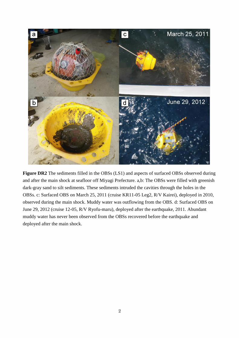
Figure DR2 The sediments filled in the OBSs (LS1) and aspects of surfaced OBSs observed during

and after the main shock at seafloor off Miyagi Prefecture. a,b: The OBSs were filled with greenish

dark-gray sand to silt sediments. These sediments intruded the cavities through the holes in the

OBSs. c: Surfaced OBS on March 25, 2011 (cruise KR11-05 Leg2, R/V Kairei), deployed in 2010,

observed during the main shock. Muddy water was outflowing from the OBS. d: Surfaced OBS on

June 29, 2012 (cruise 12-05, R/V Ryofu-maru), deployed after the earthquake, 2011. Abundant

muddy water has never been observed from the OBSs recovered before the earthquake and

deployed after the main shock.

3

Figure DR3 The 8 sediment core samples off Miyagi Prefecture. The soft sediment layers were

observed at the top of 4 core samples which were collected below 1000 m in water depth.

Additionally, accumulated remains of brittle stars occur in MC08 core sample at the interval of 6-8

cm sample below seafloor, which could imply that the newly emplaced sediment layer was 6-8 cm

thick in MC08 core sample. Left: X-ray CT images (WL: 900, WW: 1600), right: geologic columns.

The site position of the sediment cores, OBPs and OBSs are described in the lower index map. (R)

means ROV recovery. Seafloor map is made from J-EGG500 data.

4

Figure DR4 Characteristics of the sediments that filled the OBSs. The sediments became gradually

finer toward offshore on the continental slope from 300 to 1100 m in depth, whereas they coarsened

toward a fringe of the downslope basin (1100 to 1400 m deep). Black circle: Data point (OBS

positions). a: Mean grain-size (phi), b: Sand content (vol%), c: Coefficient of variance

(dimensionless sorting value), and d: Maximum grain size (phi). These Figures were illustrated

using linear approximation.

5

Figure DR5 Grain-size distributions and change patterns of the sediments that filled the OBSs off

Sendai Bay. Left: Grain size distribution of the sediments off Sendai Bay. The sediments are

composed of particles with a wide range of grain size. Right: Grain-size segregation curve

(Akiyama et al., 2007).The coarse-grained fraction of sediments can be seen to have changed

notably.

6

Figure DR6 The maximum slope gradient and sub-bottom profile in this area where OBPs and

OBSs were deployed. a: Maximum slope gradient in the area where OBPs and OBSs were deployed.

Submarine canyons and distinct gullies are not recognizable. This figure is made from J-EGG500

data. b: Sub-bottom profiling image along the white line in upper figure. Submarine slump scars

and submarine landslides are not detected in this area after the earthquake. This profiling data were

acquired in July 2012 using a parametric sub-bottom profiler (TOPAS PS 18, Kongsberg) which

Kaiyo Maru No.7 is equipped with.

7

Figure DR7 The calculated maximum flow velocity and friction velocity of Tohoku-Oki tsunami

off the Tohoku region using the numerical tsunami model by Sugawara and Goto (2012) (modified

from Fig. 6 and 9 in Sugawara and Goto, 2012). a: The calculated maximum flow velocity of the

Tohoku-Oki tsunami. The maximum flow velocity of the tsunami showed the highest value between

0–200 m in depth. b: Maximum friction velocity of the tsunami at CD line of a and suspension

threshold velocity. It is inferred that 0.5–2.5 phi sandy sediment was suspended by the flow.

8

Figure DR8 The estimated flow conditions of the body of the turbidity current on the basis of

the quasi-steady flow model of Sequeiros (2012). This figure indicates the thickness h against

the maximum suspended sediment concentration cc at the current body for different maximum

flow velocities up = 2.3, 3.5, 5.0, 6.5, 8.0, 10.0, 15.0, 20.0 m/s. When we suppose that the

sheet-like turbidity current was 20 m in thickness (Straub and Mohrig, 2009) and less than 9%

in sediment concentration (Bagnold, 1954), the velocity of the body of the turbidity current can

be estimated as ~8.0 m/s in maximum.

2. Supplementary Tables

Position

type

OBS LS1 38.6841 142.4606 1112 Recovery Pop-up ―

LS2 38.9168 142.5000 1194 Recovery Pop-up ―

LS3 38.7662 142.8331 1403 Recovery Pop-up ―

LS4 38.2997 142.6996 1409 Recovery Pop-up ―

S01 38.3502 142.1169 524 Recovery Pop-up ―

S02 37.9836 142.0827 538 Recovery Pop-up ―

S03 38.1834 142.3997 1052 Recovery Pop-up ―

S04 38.5021 142.5004 1099 Recovery Pop-up ―

S05 37.9518 142.4838 1067 Deployment No recovery ―

S08 38.1339 142.7492 1532 Recovery Pop-up ―

S09 38.1974 143.1321 2041 Recovery Pop-up ―

S10 38.4984 143.0342 1981 Recovery Pop-up ―

S14 38.5138 142.7457 1459 Recovery Pop-up ―

S15 38.3138 142.9276 1454 Recovery Pop-up ―

S17 38.5627 143.2501 2268 Deployment No recovery ―

S18 38.3174 143.2987 2773 Recovery Pop-up ―

S21 38.4319 142.0019 358 Recovery Pop-up ―

S22 38.2292 141.9838 299 Recovery Pop-up ―

S27 38.6003 142.1501 545 Recovery Pop-up ―

OBP GJT3 38.2945 143.4814 3293 Installation Pop-up ―

P02 38.5002 142.5016 1104 Installation Pop-up ―

38.1834 142.3998 1052 Installation ― ― Installed position of OBP-P03

38.1819 142.4132 1061 ROV recovery ROV ―　(moved) Recovery position of OBP-P03

P06 38.6340 142.5838 1254 Installation Pop-up ―

P07 38.0016 142.4495 1056 ROV recovery ROV 12.8

P08 38.2830 142.8320 1415 ROV recovery ROV 14.9

P09 38.2649 143.0003 1547 ROV recovery ROV 6.5

TJT1 38.2095 143.7959 5771 Installation Pop-up ―

Table DR1 Positions of OBSs and OBPs and data on the buried thickness of the sediment (Ito et al.,

2013; Suzuki et al., 2012). Position of installation is the ship position when the OBP was installed.

Position of deployment and pop-up recovery are based on several transponder measurements at three

ship positions (Ito et al., 2011). The accuracy of the data for the installation is several hundred meters,

while that of pop-up recovery and deployment is several ten meters. The accuracy of ROV recovery is

several meters. The buried thickness is the thickness of the sediment to which the OBPs were buried,

based on the depth of the bottom of the OBP when recovered by the ROV.

9

Remark

P03

TypeRecovery

method

Buried

thickness (cm)

Longitude

(degree E)

Latitude

(degree N)Depth (m)Name

Position

type OBS OBP

Sediment

coreMC01 38.1198 142.9015 1657 Ship ― ― 8

MC02 38.1831 142.4000 1059 Ship OBS-S03 OBP-P03 3.5Nearest the displaced

OBP-P03 site

MC03 38.2292 141.9834 307 Ship OBS-S22 ― ?

MC07 38.4992 142.5014 1113 Ship OBS-S04 OBP-P02 6

MC08 38.6004 142.1524 555 Ship OBS-S27 ― 7 ?Brittle stars were

buried.

MC09 38.3996 142.7807 1467 Ship ― ― 9.5

MC10 38.4333 142.0013 363 Ship OBS-S21 ― ?

MC11 38.4485 141.7503 169 Ship ― ― ?

10

Table DR2 Positions of sediment core samples and data on thickness of soft sediment layers.

Position of ship is the ship position when the multiple core sampler arrived at the bottom. The

accuracy of the data for the ship is from several ten to several hundred meters.

RemarkType NameLatitude

(degree N)

Longitude

(degree E)Depth (m)

OBS, OBP near each site Thickness of soft

sediment layer

Table DR3 Statistics of the grain-size distributions of the sediment, which filled the OBSs.

Position

name

Mean grain

size (phi)

Sorting

(phi)CV

Sand

content (%)

Maximum

grain size (phi)

LS1 5.45 1.74 0.319 22.4 0.578

LS2 5.59 1.60 0.287 18.2 0.744

LS3 5.34 1.97 0.369 25.7 0.578

LS4 5.61 1.73 0.308 17.3 0.578

S01 3.27 1.72 0.526 77.4 0.246

S02 2.34 1.77 0.757 85.8 0.080

S03 4.92 1.91 0.388 34.3 0.744

S04 5.86 1.48 0.252 10.0 0.744

S08 4.87 2.02 0.414 37.2 0.578

S09 3.93 2.21 0.563 59.0 0.412

S10 5.39 1.84 0.341 20.8 0.578

S14 5.15 1.88 0.365 27.0 0.578

S15 4.75 2.28 0.479 35.7 0.080

S18 5.81 1.58 0.273 12.2 0.744

S21 3.49 1.67 0.479 75.7 -0.086

S22 2.77 1.95 0.706 78.2 -0.086

S27 5.09 1.77 0.349 29.2 0.246

11

12

3. Supplementary methods and results

3.1 Processing procedures of data recorded in the OBPs and OBSs

Dense networks of ocean bottom pressure recorders (OBPs) and ocean bottom seismometers

(OBSs) off Miyagi for detecting seafloor movement and monitoring the seismicity due to interplate

slip events have been operated by Tohoku University since before the 2011 Tohoku-Oki earthquake

(Hino et al., 2009; Suzuki et al., 2012). Fig. 1 shows the distribution of 8 OBPs and 19 OBSs off

Miyagi.

The OBPs are of the free-fall/pop-up type, 0.6-m long, 0.6-m wide, and 0.5-m high and have a

submerged weight of 41.6 kg with grid-like anchors. The OBPs measure the water pressure and

water temperature at the seafloor every second using Digiquartz pressure sensors (Paroscientific,

Inc). The raw water pressure data recorded by OBPs were de-tided by subtracting modeled ocean

tide variations estimated by NAO.99Jb (Matsumoto et al., 2000). To understand the detailed

processes during the eastward drifting of OBP-P03, short period fluctuations of water pressure

records were investigated. To remove long period and large amplitude variation due to downslope

transport of OBP-P03, moving-averaged data (window length 59 s) were subtracted from the

de-tided water pressure data. The residual fluctuations of water pressure data are shown in Fig. 3.

Note that OBP temperature records cannot follow the rapid temperature change of the surrounding

water because the temperature sensor is a built-in sensor to compensate for thermal effects on the

quartz-crystal pressure transducer (Yilmaz et al., 2004). Therefore, the actual water temperature

may have increased and decreased much more rapidly than observed temperature variation (Schaad,

personal communication).

The OBSs are of the free-fall/pop-up type, ~0.5-m long, 0.5-m wide, and 0.5-m high and have a

submerged weight of ~28 kg with square anchors. The OBSs measure ground velocity at rate of 100

or 128 samples per second using short-period (1 or 4.5 Hz) three-component geophones. In this

study, only the vertical component of the ground velocity data was used. A band-pass filter (2–8

13

Hz) was applied to the vertical component records. The 128-Hz sampled data were resampled to

100 Hz.

3.2 Grain-size analysis

The characteristics and spatial variation in the sediments collected by 17 OBSs were determined

by grain-size analysis using laser diffraction and a scattering particle-size analyzer. Grain-size

distributions of the 17 samples taken from inside the OBSs were analyzed using a Mastersizer 2000

laser granulometer (Malvern Instruments, Malvern, UK) in the Center for Advanced Marine Core

Research, Kochi University. We used hexametaphosphoric acid sodium salt as a dispersant and

ultrasonic bath for 5 min to scatter the fine sediments (Sperazza et al., 2004). Measured values of

grain diameter were converted to the phi scale. The mean grain-size (M) and sorting coefficient (σ)

were calculated on the basis of the moment method (Folk, 1966; Harrington, 1968) as follows:

100

pdM

(1)

2

100

p d M

(2)

where d is a representative value of each grain-size class (in increments of ~0.167 phi) and p is

volume fraction (in percent). The coefficient of variance of grain-size distribution (CV), which is a

dimensionless of sorting, is defined as follows:

CVM

(3)

The sand content is volume fraction of sand (> 4 phi, 63 μm) in grain-size distributions (vol%).

The maximum grain size is maximum grain size class (phi) in grain-size distributions.

To illustrate the spatial variation of grain-size distribution curves, the “grain-size segregation

curve” is employed herein (Akiyama et al., 2007). The grain-size segregation curves indicate the

14

results of comparison between two different grain-size distribution curves. Here, Di is a

representative grain diameter of the i-th grain-size class in phi scale, and iF D is the volume

percentage of sediment in the i-th class grain-size fraction. The grain-size segregation curve

21 iS D of two grain-size distributions 1 iF D and 2 iF D (where F2 is farther offshore than

F1) is defined as follows.

2

21 10

1

logi

i

i

F DS D

F D

(4)

Thus, if volume percentage of the grain-size distribution 1 iF D is larger than that of 2 iF D ,

the value of grain-size segregation curve 21 iS D becomes negative. In contrast, if 1 iF D is

smaller than 2 iF D , 21 iS D becomes positive. It should be noted that 21 iS D is not defined

at the grain-size class where 1 iF D or 2 iF D is zero.

3.3 Analysis and results of the sediment core samples

Sampling seafloor sediment was conducted by R/V Tansei-maru (Cruise KT-12-9) over range of

water depth 170 – 1700 m off Miyagi Prefecture in May, 2012. 8 sediment core samples were

collected using a multiple-core sampler (82 mm in diameter, Rigosha) without disturbance of

surface sediments (Fig. DR3; Table DR2). Sediment core samples were described sedimentary

structures by naked eyes and carried out X-ray CT analysis (RADIX-PRATICO, FR version,

Hitachi Medical Corporation) in the Center for Advanced Marine Core Research, Kochi University.

Soft sediment layers (new sediment layer) were observed at the top of 4 core samples which

were collected below 1000 m in water depth. Sediment layers ranges 3.5–9.5 cm in thickness and

are composed of normally graded sandy silt – clayey silt with high water content. Basal part of the

layers generally consists of a graded and/or laminated thin sandy layer. The soft sediment layers are

15

less bioturbated than lower historical layers, and their boundaries are sharp. These layers can be

interpreted as newly emplaced muddy turbidites of which graded bedding in one of typical features

(Walker, 1967). MC01 and MC09 core samples contain a few soft sediment layers, and are thicker

than that MC02 and MC07. By contrast, the sediment samples at shallower than 600 m in water

depth are composed of heavily bioturbated sandy sediments. Because of their intense bioturbation,

soft sediment layer cannot be distinguished from historical layers. However, accumulated remains

of brittle stars occur in MC08 core sample at the interval of 6-8 cm sample below seafloor, which

could imply that the newly emplaced sediment layer was 6-8 cm thick in MC08 core sample.

3.4 Analysis of critical flow velocities for suspended sediment load

It is known that sediments are entrained as suspended load when the friction velocity of flows

exceeds the settling velocity of sediment particles (Bagnold, 1966):

* 1s

u

w (5)

where *u is the friction velocity, and sw is the particle settling velocity. sw is calculated using a

relationship for natural sand (Dietrich, 1982).

s fw R RgD (6)

where R is the submerged specific gravity of sediment (1.65 for quartz)

2 3 4

1 2 3 4 5f p p p pR exp b b log Re b log Re b log Re b log Re

(7)

and b1 = 2.891394, b2 = 0.95296, b3 = 0.056835, b4 = 0.002892, b5 = 0.000245.

The calculated critical friction velocities of each grain-size particle for the onset of suspension are

0.26 m/s (-1 phi), 0.14 m/s (0 phi), 0.061 m/s (1 phi), 0.024 m/s (2 phi), 0.0079 m/s (3 phi), and

0.0023 m/s (4 phi), respectively.

16

3.5 Critical flow velocity for transporting the OBP-P03

In this case, the OBP is assumed to be a boulder-sized spherical clast. Thus the OBP can be

displaced when the drag force FD exceeds the maximum frictional force Fμ at the bottom.

Drag force FD is given (Bradley and Mears, 1980)

2

2

f

D D n

uF C A

(8)

where CD is the drag coefficient, An is the area of the particle projected normal to the flow, ρf is

mass of unit volume of the sea water and u is flow velocity.

The normal frictional force Fμ is given (Kabardin, 1990)

F mg (9)

where μ is the coefficient of friction; m is the mass of the partly submerged boulder (in this case, the

OBP); and g is the acceleration due to gravity.

Balancing equations (8) and (9), the flow velocity required for moving boulders (OBP) is

defined as follows (Paris et al., 2010):

2

D n f

mgu

C A

(10)

where CD = 0.4 (Parker, 2005), An = 0.2670 m2 (the smallest area of the OBP), ρf = 1024 kg/m

3, μ =

0.7 (Noormets et al., 2004), m = 41.6 kg, and g = 9.81 m/s2. The minimum flow velocity required to

move the OBP is estimated to be 2.3 m/s.

17

3.6 Estimation of migration rate of the turbidity current

(1) Averaged velocity and flow condition at the current head

The averaged head velocity is estimated, under the assumption that the turbidity current arrived

at OBP-P03 position over a period of 3 h from depths of 100–450 m. The distance up to the final

OBP-P03 position is ~77 km from a depth of 100 m, and ~26 km from a depth of 450 m in depth. It

is assumed that the turbidity current traveled these distances for 3 h to reach the final OBP-P03

position. Hence, the averaged head velocity is estimated to be 7.1 m/s and 2.4 m/s from depths of

100 and 450 m, respectively.

The characteristics of the turbidity current such as flow thickness and concentration are

estimated using the estimated averaged head velocity. It is known empirically that the densimetric

Froude number Frd of the current head is constant at 1.2 regardless of slope gradients (Huppert and

Simpson, 1980). Densimetric Froude number Frd is given by:

1 2d

UFr .

RgCh (11)

where U is the layer-averaged head velocity of turbidity current; C is the layer-averaged

concentration of suspended sediment at the current head; and h is the thickness of the head.

Equation (11) is transposed to obtain the following:

2

2

rd

UCh

F Rg (12)

Substituting the estimated averaged head velocity (7.1 m/s and 2.4 m/s) in Equation (12) yields =

2.2 and 0.25, respectively. Thus, the sediment concentration C is estimated to have been 0.2–9.0%

when the thickness of head of turbidity current h was 3–150 m.

18

(2) Flow condition at current body

The condition at the current body is estimated by the method of Sequeiros (2012) that assumes

the body of the turbidity current was nearly quasi-steady condition. The method is based on the

predictive equation (13) that returns the densimetric Froude number Frd of the current body as a

function of the average bed slope, the combined friction factor, and the ratio between the settling

velocity of the suspended sediment and the shear velocity of the current (Sequeiros, 2012)

1.1

0.210.75

*

0.15 tanh 7.62 1 1sd fFr S C

u

(13)

where S is the average bed slope, νs is the fall velocity of characteristic grain size, u* is the shear

velocity, Cf is the friction coefficient, α is the ratio between bed shear stress and interface shear

stress. There are other characteristic flow parameters that show a strong dependency on the

densimetric Froude number, equations (14) – (19) (Sequeiros, 2012).

3 950 15 .

d. Fr (14)

0 580 42p .

d

z. Fr

h

(15)

1 301 15 0 14p .

d

u. . Fr

U (16)

2 800 09 .cd

z. Fr

h

(17)

2 901 15 0 20 .cd

c. . Fr

C (18)

0 210 78 .

d

i

h. Fr

z

(19)

where zp is the distance from the bed to point of maximum velocity, up is maximum (peak) velocity,

zc is the distance from the bed to the point below maximum volume concentration, cc is the

19

maximum volume concentration, C is the layer-averaged suspend sediment concentration of the

current, zi is the distance from the bed to the current interface.

The condition such as velocity, thickness and concentration at the current body is estimated by

implicit model using equations (13)-(19) (Sequeiros, 2012). Input parameters are substituted

average bed slope S = water depth / distance = (1061 – 450)/2600 = 0.0235, the bed roughness ks =

0.1 m, the ratio of characteristic setting velocity to shear velocity νs/u* = 0.002 (Sequeiros, 2012).

The range of conditions at current body are estimated by varying the variables, the distance from

the bed to the current interface zi and the layer-averaged fractional excess density of the current

. The estimated conditions at the current body are shown in Fig. DR8, when the velocity in

maximum up are 2.3, 3.5, 5.0, 6.5, 8.0, 10.0, 15.0, 20.0 m/s. The lowest velocity corresponds to the

minimum velocity estimated by the critical flow velocity for transporting the OBP-P03. In addition,

when we suppose that the flow was 20 m which is the minimum thickness of the sheet-like turbidity

current (estimated at Brunei Darussalam by Straub and Mohrig, (2009) and less than 9% in

sediment concentration (Bagnold, 1954), the velocity of the body of the turbidity current can be

estimated as ~8.0 m/s in maximum, and ~5.6-5.8 m/s in layer-averaged velocity.

REFERENCE

Akiyama, M., Naruse, H., and Masuda, F., 2007, Detailed grain size analysis of the flood deposits

of the Yayoi Period in Shirakawa Fan: application of grain size segregation analysis to the

subaerial debris flow and hyperconcentrated flow deposit (in Japanese): the Sedimentological

Society of Japan Annual Meeting, Tsukuba, Abstracts, p. 48.

20

Bagnold, R. A., 1954, Experiments on a gravity-free dispersion of large solid spheres in a

Newtonian fluid under shear: Proceedings of the Royal Society of London, v. A225, p. 49–63,

doi:10.1098/rspa.1954.0186.

Bagnold, R. A., 1966, An approach to the sediment transport problem for general physics:

Washington, D. C., U.S. Geological Survey Professional Paper, v. 422-I.

Bradley, W. C. and Mears, A. I., 1980, Calculations of flows needed to transport coarse fraction of

Boulder Creek alluvium at Boulder, Colorado: summary: Geological Society of America

Bulletin, Part I 91, p. 135–138, doi:10.1130/GSAB-P2-91-1057.

Dietrich, W. E., 1982, Settling velocity of natural particles: Water Resource Research, v. 18, p.

1615-1626, doi:10.1029/WR018i006p01615.

Folk, R. L., 1966, A review of grain-size parameters: Sedimentology, v. 6, p. 73–93,

doi:10.1111/j.1365-3091.1966.tb01572.x.

Harrington, R. F., 1968, Field Computation by Moment Methods, 1st ed: New York, The

Macmillan Co.

Hino, R., Ii, S., Iinuma, T. and Fujimoto, H., 2009, Continuous long-term seafloor pressure

observation for detecting slow-slip interplate events in Miyagi-Oki on the landward Japan

Trench slope: Journal of Disaster Research, v. 4, p. 72–82.

Huppert, H. E. and Simpson, J. E., 1980, The slumping of gravity currents: Journal of Fluid

Mechanics, v. 99, p. 785–799, doi:10.1017/S0022112080000894.

Ito, Y., Hino, R., Kido, M., Fujimoto, H., Osada, Y., Inazu, D., Ohta, Y., Iinuma, T., Ohzono, M.,

Miura, S., Mishina, M., Suzuki, K., Tsuji, T., and Ashi, J., 2013, Episodic slow slip events in

21

the Japan subduction zone before the 2011 Tohoku-Oki earthquake: Tectonophysics, v. 600, p.

14–26, doi:10.1016/j.tecto.2012.08.022.

Ito, Y., Tsuji, T., Osada, Y., Kido, M., Inazu, D., Hayashi, Y., Tsushima, H., Hino R., and Fujimoto,

H., 2011, Frontal wedge deformation near the source region of the 2011 Tohoku-Oki

earthquake: Geophysical Research Letter, v. 38, L00G05, doi:10.1029/2011GL048355.

Kabardin, O., 1990, Koolifüüsika käsiraamat: Valgus, Tallinn, 320p.

Matsumoto, K., Takanezawa, T. and Ooe, M., 2000, Ocean tide models developed by assimilating

TOPEX/POSEIDON altimeter data into hydrodynamical model: a global model and a

regional model around Japan: Journal of Oceanography, v. 56, p. 567–581, doi:

10.1023/A:1011157212596.

Noormets, R., Crook, K. A. W. and Felton, E. A., 2004, Sedimentology of rocky shorelines: 3:

hydrodynamics of megaclast emplacement and transport on a shore platform, Oahu, Hawaii:

Sedimentary Geology, v. 172, p. 41–65, doi:10.1016/j.sedgeo.2004.07.006.

Paris, R., Fournier, J., Poizot, E., Etienne, S., Morin, J., Lavigne, F., and Wassmer, P., 2010,

Boulder and fine sediment transport and deposition by the 2004 tsunami in Lhok Nga

(western Banda Aceh, Sumatra, Indonesia): a coupled offshore-onshore model: Marine

Geology, v. 268, p. 43–54, doi:10.1016/j.margeo.2009.10.011.

Parker, G., 2005, 1D sediment transport morphodynamics with applications to rivers and turbidity

currents. http://hydrolab.illinois.edu/people/parkerg//morphodynamics_e-book.htm (November

2012).

22

Schaad, T., personal communication.

Sequeiros, O. E. 2012, Estimating turbidity current conditions from channel morphology: A Froude

number approach: Journal of Geophysical Research, v. 117, C04003,

doi:10.1029/2011JC007201.

Sperazza, M., Moore J. N. and Hendrix M.S., 2004, High-resolution particle size analysis of

naturally occurring very fine-grained sediment through laser diffractometry: Journal of

Sedimentary Research, v. 74, p. 736–743, doi:10.1306/031104740736.

Straub, K. M., and Mohrig, D., 2009, Constructional canyons built by sheet-like turbidity currents:

observations from offshore Brunei Darussalam: Journal of Sedimentary Research, v. 79, p.

24–39, doi:10.2110/jsr.2009.006.

Sugawara, D., and Goto, K., 2012, Numerical modeling of the 2011 Tohoku-oki tsunami in the

offshore and onshore of Sendai Plain, Japan: Sedimentary Geology, v. 282, p. 110–123,

doi:10.1016/j.sedgeo.2012.08.002.

Suzuki, K., Hino, R., Ito, Y., Yamamoto, Y., Suzuki, S., Fujimoto, H., Shinohara, M., Abe, M.,

Kawaharada, Y., Hasegawa, Y., and Kaneda, Y., 2012, Seismicity near the hypocenter of the

2011 off the Pacific coast of Tohoku earthquake deduced by using Ocean Bottom

Seismographic data: Earth, Planets and Space, v. 64, p. 1125–1135,

doi:10.5047/eps.2012.04.010.

23

Walker, R. G., 1967, Turbidite sedimentary structures and their relationships to proximal and distal

depositional environment: Journal of Sedimentary Petrology, v. 37, p. 25–43.

Yilmaz, M., Migliacio, P. and Bernard, E., 2004, Broadband vibrating quartz pressure sensors for

tsunameter and other oceanographic applications: Proceeding of Oceans 2004 Marine

Technology Society IEEE Techno-Ocean 2004, p. 1381–1387,

doi:10.1109/OCEANS.2004.1405783.