gs01 0163 analysis of microarray...
TRANSCRIPT

GS01 0163Analysis of Microarray Data
Keith Baggerly and Bradley BroomDepartment of Bioinformatics and Computational Biology
UT M. D. Anderson Cancer [email protected]@mdanderson.org
24 November 2009

INTRODUCTION TO MICROARRAYS 1
Lecture 25: SNP Arrays
• SNPs, GWAS, HapMap project
• Affymetrix SNP Arrays
c© Copyright 2004–2009, KR. Coombes, KA. Baggerly, and BM. Broom GS01 0163: ANALYSIS OF MICROARRAY DATA

INTRODUCTION TO MICROARRAYS 2
Single Nucleotide Polymorphisms (SNPs)
Two unrelated people share about 99.5% of their DNAsequence.
One of the most common differences is that at specific sitessome people may have (for instance) a G, while others mighthave an A. These sites are called single nucleotidepolymorphisms, or SNPs.
Each of the two bases that can occur at the SNP is called anallele. (A third or even fourth allele is possible, but veryuncommon. We will ignore the possibility hereafter.)
By convention, the most common allele at each SNP is calledA and the less common SNP is called B.
c© Copyright 2004–2009, KR. Coombes, KA. Baggerly, and BM. Broom GS01 0163: ANALYSIS OF MICROARRAY DATA

INTRODUCTION TO MICROARRAYS 3
Genotypes
Since there are two copies of each chromosome (except forX and Y in males), there are three possible pairs of alleles foreach SNP: AA, AB, and BB.
For each SNP, an individual’s genotype is the specificcombination of alleles that it possesses.
c© Copyright 2004–2009, KR. Coombes, KA. Baggerly, and BM. Broom GS01 0163: ANALYSIS OF MICROARRAY DATA

INTRODUCTION TO MICROARRAYS 4
Haplotypes
Chromosomes are not inherited as indivisible units. Througha process known as recombination the descendant’schromosome contains segments of DNA taken randomlyfrom the two different parent chromosomes.
Segments of DNA that are far apart are inheritedindependently, whereas segments that are close togethertend to be inherited together.
Segments that are common to many people are calledhaplotypes. The distribution of haplotypes varies betweenpopulations and geographic regions.
Sequences of adjacent SNPs can be used to modelhaplotypes.
c© Copyright 2004–2009, KR. Coombes, KA. Baggerly, and BM. Broom GS01 0163: ANALYSIS OF MICROARRAY DATA

INTRODUCTION TO MICROARRAYS 5
Genome-wide Association Studies
Many genome-wide association and gene-environmentinteraction studies are being undertaken in order to findgenes associated with complex, heritable disorders, includingcancer.
Since there are about 10 million common SNPs, testing everyindividual for all SNPs would have been extremely expensive.(NGS might change that.)
By identifying tag SNPs that uniquely identify the commonhaplotypes, much less testing is required.
It is estimated that about 300,000 to 600,000 tag SNPscontain most of the information about the patterns of geneticvariation.
c© Copyright 2004–2009, KR. Coombes, KA. Baggerly, and BM. Broom GS01 0163: ANALYSIS OF MICROARRAY DATA

INTRODUCTION TO MICROARRAYS 6
International HapMap Project
The International HapMap project is a recent, large-scaleeffort to facilitate GWAS studies:
• Phase 1: 269 samples, 1.1 M SNPs
• Phase 2: 270 samples, 3.9 M SNPs
• Phase 3: 1115 samples, 1.6 M SNPs
Phase 3 platforms:
• Illumina Human1M (by Wellcome Trust Sanger Institute)
• Affymetrix SNP 6.0 (by Broad Institute)
c© Copyright 2004–2009, KR. Coombes, KA. Baggerly, and BM. Broom GS01 0163: ANALYSIS OF MICROARRAY DATA
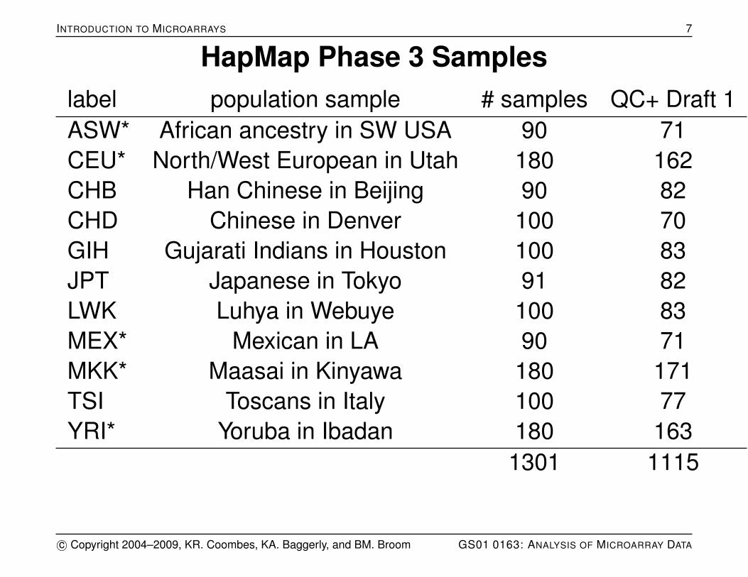
INTRODUCTION TO MICROARRAYS 7
HapMap Phase 3 Sampleslabel population sample # samples QC+ Draft 1ASW* African ancestry in SW USA 90 71CEU* North/West European in Utah 180 162CHB Han Chinese in Beijing 90 82CHD Chinese in Denver 100 70GIH Gujarati Indians in Houston 100 83JPT Japanese in Tokyo 91 82LWK Luhya in Webuye 100 83MEX* Mexican in LA 90 71MKK* Maasai in Kinyawa 180 171TSI Toscans in Italy 100 77YRI* Yoruba in Ibadan 180 163
1301 1115
c© Copyright 2004–2009, KR. Coombes, KA. Baggerly, and BM. Broom GS01 0163: ANALYSIS OF MICROARRAY DATA

INTRODUCTION TO MICROARRAYS 8
Data Access
Unlike the TCGA SNP data, the HapMap project data isavailable fromhttp://hapmap.ncbi.nlm.nih.gov/downloads/raw data/?N=D.
We will use the CUPID.tgz dataset in thehapmap3 affy6.0 subdirectory. This archive contains 77CEL files from the Affymetrix SNP 6.0 platform.
c© Copyright 2004–2009, KR. Coombes, KA. Baggerly, and BM. Broom GS01 0163: ANALYSIS OF MICROARRAY DATA

INTRODUCTION TO MICROARRAYS 9
Affymetrix SNP Chips
Mapping 10K (1 array, 18 µm feature size)
Mapping 10K v2.0
Mapping 100K (2 arrays, 8 µm feature size)
Mapping 500K (250K Nsp and 250K Sty, 5 µm feature size)
SNP 5.0
SNP 6.0
c© Copyright 2004–2009, KR. Coombes, KA. Baggerly, and BM. Broom GS01 0163: ANALYSIS OF MICROARRAY DATA

INTRODUCTION TO MICROARRAYS 10
Affymetrix SNP 6.0
More than 906,600 SNPs:
• Approx. 482,000 SNPs derived from previous generationarrays
• Additional tag SNPs from early phase of HapMap project
More than 946,000 probes for detecting copy numbervariation:
• 202,000 probes targetting 5,677 known regions of copynumber variation
• more than 744,000 additional evenly spaced SNPs toenable detection of novel copy number variation
c© Copyright 2004–2009, KR. Coombes, KA. Baggerly, and BM. Broom GS01 0163: ANALYSIS OF MICROARRAY DATA
INTRODUCTION TO MICROARRAYS 11
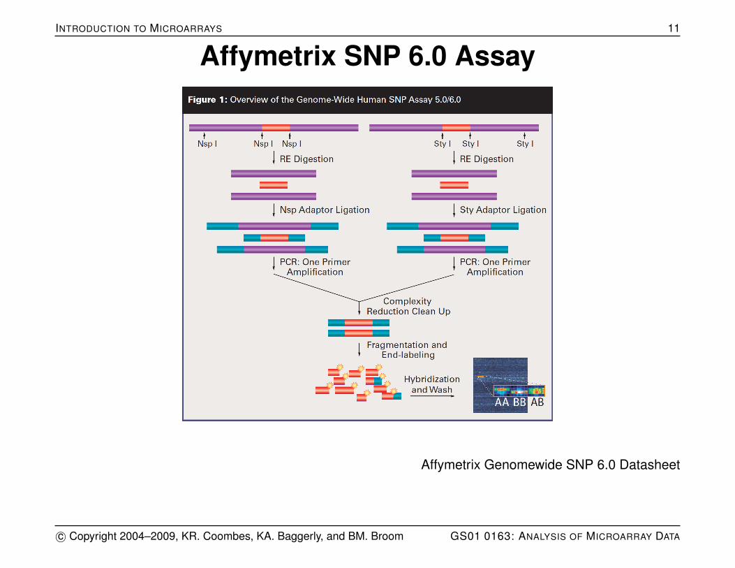
Affymetrix SNP 6.0 Assay
Affymetrix Genomewide SNP 6.0 Datasheet
c© Copyright 2004–2009, KR. Coombes, KA. Baggerly, and BM. Broom GS01 0163: ANALYSIS OF MICROARRAY DATA
INTRODUCTION TO MICROARRAYS 12
SNP Chip Design
The SNP chip’s basic design is similar to that of expressionarrays, in that an array of 25 bp oligonucleotide sequences(features) is laid across the surface of the chip. The sample’sDNA is amplified, a marker is attached, and hybridized to thearray. The array is scanned to quantify the relative amount ofsample bound to each feature.
For SNPs, there is a pair of probes: one for each of thealleles.
For non-polymorphic CNV probes, there is just a singleprobe.
On early chips there were both PM and MM probes for eachof the two alleles, making a quartet.
c© Copyright 2004–2009, KR. Coombes, KA. Baggerly, and BM. Broom GS01 0163: ANALYSIS OF MICROARRAY DATA

INTRODUCTION TO MICROARRAYS 13
Early chips contained multiple quartets per SNP at differentoffsets (e.g. -4, -2, -1, 0, 1, 3, 4) to the SNP’s location.
Recent chips just use two replicates of the PM pair that bestdistinguishes the two alleles.
c© Copyright 2004–2009, KR. Coombes, KA. Baggerly, and BM. Broom GS01 0163: ANALYSIS OF MICROARRAY DATA

INTRODUCTION TO MICROARRAYS 14
Genotyping Algorithms
ABACUS
MPAM (Affy 10k)
DM (Affy 100k)
BRLMM (Affy 500k)
Birdseed (Affy SNP 6.0)
CRLMM
c© Copyright 2004–2009, KR. Coombes, KA. Baggerly, and BM. Broom GS01 0163: ANALYSIS OF MICROARRAY DATA
INTRODUCTION TO MICROARRAYS 15
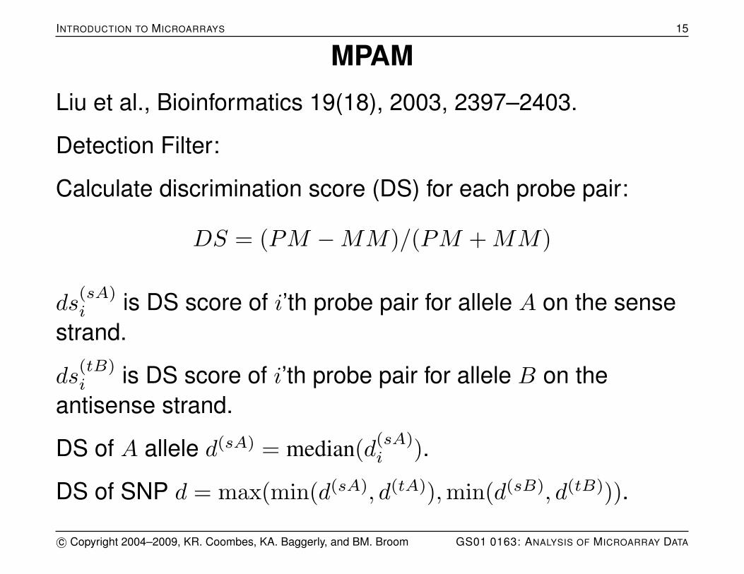
MPAM
Liu et al., Bioinformatics 19(18), 2003, 2397–2403.
Detection Filter:
Calculate discrimination score (DS) for each probe pair:
DS = (PM −MM)/(PM +MM)
ds(sA)i is DS score of i’th probe pair for allele A on the sense
strand.
ds(tB)i is DS score of i’th probe pair for allele B on the
antisense strand.
DS of A allele d(sA) = median(d(sA)i ).
DS of SNP d = max(min(d(sA), d(tA)),min(d(sB), d(tB))).
c© Copyright 2004–2009, KR. Coombes, KA. Baggerly, and BM. Broom GS01 0163: ANALYSIS OF MICROARRAY DATA

INTRODUCTION TO MICROARRAYS 16
Feature Extraction
Relative allele signal (RAS) for the ith probe quartet of thesense strand:
s(s)i = A
(s)i /(A(s)
i +B(s)i )
whereA
(s)i = max(PM (sA)
i −MM(s)i , 0)
B(s)i = max(PM (sB)
i −MM(s)i , 0)
MM(s)i = (MM
(sA)i +MM
(sB)i )/2
RAS for sense strand s(s) = median(s(s)i )
RAS for antisense strand s(t) = median(s(t)i )
c© Copyright 2004–2009, KR. Coombes, KA. Baggerly, and BM. Broom GS01 0163: ANALYSIS OF MICROARRAY DATA

INTRODUCTION TO MICROARRAYS 17
Feature Space
The pair (s(s), s(t)) is a point in a unit square feature space.
Points close to (1, 1) should be AA.
Points close to (0, 0) should be BB.
Points close to (0.5, 0.5) should be AB.
c© Copyright 2004–2009, KR. Coombes, KA. Baggerly, and BM. Broom GS01 0163: ANALYSIS OF MICROARRAY DATA

INTRODUCTION TO MICROARRAYS 18
Genotype Clusters are SNP Dependent
In real data, the locations, sizes, and shapes of the genotypeclusters depend on the SNP concerned:
• affinity of target and probe depend on the sequence,
• cross hybridization.
Therefore, genotype cluster regions must be estimated forevery SNP separately using a large training data set.
c© Copyright 2004–2009, KR. Coombes, KA. Baggerly, and BM. Broom GS01 0163: ANALYSIS OF MICROARRAY DATA

INTRODUCTION TO MICROARRAYS 19
Classification with MPAM
For each SNP, use (modified) PAM to cluster features intraining data into k groups.
For genotyping, we expect 1 to 3 groups.
Assign genotypes based on median coordinates of theclusters.
Use average silhouette width to determine quality of theclassification.
c© Copyright 2004–2009, KR. Coombes, KA. Baggerly, and BM. Broom GS01 0163: ANALYSIS OF MICROARRAY DATA

INTRODUCTION TO MICROARRAYS 20
PAM fails with very different allele frequencies
With very different cluster sizes, PAM tends to split largestcluster:
PAM was modified to penalize small between-groupdistances.
c© Copyright 2004–2009, KR. Coombes, KA. Baggerly, and BM. Broom GS01 0163: ANALYSIS OF MICROARRAY DATA

INTRODUCTION TO MICROARRAYS 21
Post-call filter to exclude bad calls
c© Copyright 2004–2009, KR. Coombes, KA. Baggerly, and BM. Broom GS01 0163: ANALYSIS OF MICROARRAY DATA

INTRODUCTION TO MICROARRAYS 22
Dynamic Model-based Algorithm (DM)
Di et al., Bioinformatics 21(9), 2005, 1958–1963.
Introduced to overcome perceived deficiences in MPAM:
• Large number of training samples required to observe allthree phenotypes and build accurate empirical models.
• SNPs with low minor allele frequency are difficult to modelaccurately.
• Requires manual inspection of selected SNPs.
• Not flexible enough to accommodate additionalimprovements.
c© Copyright 2004–2009, KR. Coombes, KA. Baggerly, and BM. Broom GS01 0163: ANALYSIS OF MICROARRAY DATA

INTRODUCTION TO MICROARRAYS 23
DM
DM:
• aggregates multiple SNP quartets into SNP genotype calland confidence metric
• stratifies states into four models: Null, A, AB, and B.
• uses a one-sided Wilcoxon signed rank test to produce fourp-values, one for each model
DM also includes methods for SNP screening and probereduction, and enables SNP screening using a relativelysmall sample set.
c© Copyright 2004–2009, KR. Coombes, KA. Baggerly, and BM. Broom GS01 0163: ANALYSIS OF MICROARRAY DATA

INTRODUCTION TO MICROARRAYS 24
Four Models
Four states for each quartet:
Null: No probe brighter than the rest. All assumed to bebackground.
A or B: Only PM probe for A (or B) is bright. Other 3 probesassumed to be background.
AB: Both PM probes are bright. Two MM probes assumed tobe background.
Which state is most likely?
c© Copyright 2004–2009, KR. Coombes, KA. Baggerly, and BM. Broom GS01 0163: ANALYSIS OF MICROARRAY DATA

INTRODUCTION TO MICROARRAYS 25
Likelihood Models
Assume all probes in a quartet are independent, and signalintensities are i.i.d. normal random variables.
For each probe in a quartet (x = 1, 2, 3, 4):µx meanσ2
x variancenx number of pixelsµ̂x estimated mean assuming model mσ̂2
x estimated variance assuming model m
Log likelihood given by
L(m) = −12
4∑x=1
nx
[ln(2πσ̂2
x) +σ2
x + (µx − µ̂x)2
σ̂2x
]
c© Copyright 2004–2009, KR. Coombes, KA. Baggerly, and BM. Broom GS01 0163: ANALYSIS OF MICROARRAY DATA

INTRODUCTION TO MICROARRAYS 26
Estimated mean and variance for Null model
For the Null model, all probes are background and evenlydistibuted, hence:
µ̂1 = µ̂2 = µ̂3 = µ̂4 =∑4
x=1 nxµx∑4x=1 nx
σ̂21 = σ̂2
2 = σ̂23 = σ̂2
4 =∑4
x=1 nx[σ2x + µ2
x]∑4x=1 nx
− µ̂2
c© Copyright 2004–2009, KR. Coombes, KA. Baggerly, and BM. Broom GS01 0163: ANALYSIS OF MICROARRAY DATA

INTRODUCTION TO MICROARRAYS 27
Estimated mean and variance for model A
For model A, the PM for A is foreground, the other three arebackground:
µ̂1 = µ1
σ̂21 = σ2
1
µ̂2 = µ̂3 = µ̂4 =
∑x 6=1 nxµx∑
x 6=1 nx
σ̂22 = σ̂2
3 = σ̂24 =
∑x 6=1 nx[σ2
x + µ2x]∑
x 6=1 nx− µ̂2
Similarly for model B.
c© Copyright 2004–2009, KR. Coombes, KA. Baggerly, and BM. Broom GS01 0163: ANALYSIS OF MICROARRAY DATA

INTRODUCTION TO MICROARRAYS 28
Estimated mean and variance for model AB
For model AB, the PMs for A and B are foreground, the twoMM are background:
µ̂1 = µ̂3 =n1µ1 + n3µ3
n1 + n3
σ̂21 = σ̂2
3 =n1[σ2
1 + (µ̂1 − µ1)2] + n3[σ23 + (µ̂3 − µ3)2]
n1 + n3
µ̂2 = µ̂4 =n2µ2 + n4µ4
n2 + n4
σ̂22 = σ̂2
4 =n2[σ2
2 + (µ̂2 − µ2)2] + n4[σ24 + (µ̂4 − µ4)2]
n2 + n4
c© Copyright 2004–2009, KR. Coombes, KA. Baggerly, and BM. Broom GS01 0163: ANALYSIS OF MICROARRAY DATA

INTRODUCTION TO MICROARRAYS 29
SNP Level Aggregation
Different probe quartets might support different states. Needto aggregate robustly over all probe quartets.
Score for model m:
S(m) = L(m)−max{L(k), k = 1, 2, 3, 4, k 6= m}
For each model m generate a vector of the scores for all nquartets in the SNP:
Vm = {S1(m), S2(m), . . . , Sn(m)},m = Null,A,AB,B
c© Copyright 2004–2009, KR. Coombes, KA. Baggerly, and BM. Broom GS01 0163: ANALYSIS OF MICROARRAY DATA

INTRODUCTION TO MICROARRAYS 30
Finding most likely model
Use Wilcoxon signed rank test to evaluate support for eachmodel across all probe quartets.
For all 4 models, apply to hypotheses H0 : median(Si(m)) = 0versus H1 : median(Si(m)) > 0 to obtain 4 p-values.
The least p-value, provided it is below a threshold,determines the genotype call and the p-value is theconfidence of that call.
If the least p-value exceeds the threshold, or the best modelis null, the final genotype is no-call.
c© Copyright 2004–2009, KR. Coombes, KA. Baggerly, and BM. Broom GS01 0163: ANALYSIS OF MICROARRAY DATA

INTRODUCTION TO MICROARRAYS 31
BRLMM
BRLMM
• performs multiple chip analysis: simultaneous estimation ofprobe effects and allele signals for each SNP.
• estimates genotypes by a multiple-sample classification,borrowing information from other SNPs as necessary tomake better predictions.
BRLMM makes weaker assumptions about probe behavior,making it more robust on real-world data.
c© Copyright 2004–2009, KR. Coombes, KA. Baggerly, and BM. Broom GS01 0163: ANALYSIS OF MICROARRAY DATA

INTRODUCTION TO MICROARRAYS 32
BRLMM Approach
1. Normalize probe intensities and estimate allele signals foreach SNP
2. Use DM to make an initial guess at each SNPs genotype
3. Select SNPs containing a minimum number of all threegenotypes
4. Transform allele signal estimates into a better behaved 2Dspace
5. Use selected SNPs to estimate a prior distribution of typicalcluster centers and variance-covariance matrices
c© Copyright 2004–2009, KR. Coombes, KA. Baggerly, and BM. Broom GS01 0163: ANALYSIS OF MICROARRAY DATA

INTRODUCTION TO MICROARRAYS 33
6. Re-evaluate each SNP, combining initial genotype guesseswith prior information in an ad-hoc Bayesian procedure toderive a posterior estimate of cluster centers and variances
7. Determine genotype and confidence score for eachobservation based on its Mahalanobis distance from thethree cluster centers
c© Copyright 2004–2009, KR. Coombes, KA. Baggerly, and BM. Broom GS01 0163: ANALYSIS OF MICROARRAY DATA

INTRODUCTION TO MICROARRAYS 34
Normalization and Probe Intensities
Use quantile normalization at the feature level.
No background correction used. (For most fragmentscontaining SNPs, target levels are well above background.)
Use log-scale transformation for the PM intensities.
Use median polish to fit feature effects to the data and obtaina signal.
Summarize probes into two values, representing A and Bsignals.
c© Copyright 2004–2009, KR. Coombes, KA. Baggerly, and BM. Broom GS01 0163: ANALYSIS OF MICROARRAY DATA

INTRODUCTION TO MICROARRAYS 35
Clustering Space Transformation
c© Copyright 2004–2009, KR. Coombes, KA. Baggerly, and BM. Broom GS01 0163: ANALYSIS OF MICROARRAY DATA

INTRODUCTION TO MICROARRAYS 36
Clustering Space Transformation
MA transformation isolates most of the difference betweengenotypes onto the M axis, but artificially makes homozygousclusters more broadly variable than heterozygous clusters.
c© Copyright 2004–2009, KR. Coombes, KA. Baggerly, and BM. Broom GS01 0163: ANALYSIS OF MICROARRAY DATA

INTRODUCTION TO MICROARRAYS 37
Clustering Space Transformation
Transformed Contrast transformation can be used to balancethe variability in homozygous and heterozygous clusters.
c© Copyright 2004–2009, KR. Coombes, KA. Baggerly, and BM. Broom GS01 0163: ANALYSIS OF MICROARRAY DATA

INTRODUCTION TO MICROARRAYS 38
Genotyping
Model three clusters (for AA, AB, BB) defining cluster centersand covariance matrices.
Determine distance from each test point to each clustercenter using Mahalanobis distance (which takes into accountvariation and covariation in the cluster along each axis).
Confidence assigned to call is d1/d2 where d1 is the smallestdistance and d2 is the second smallest distance.
c© Copyright 2004–2009, KR. Coombes, KA. Baggerly, and BM. Broom GS01 0163: ANALYSIS OF MICROARRAY DATA
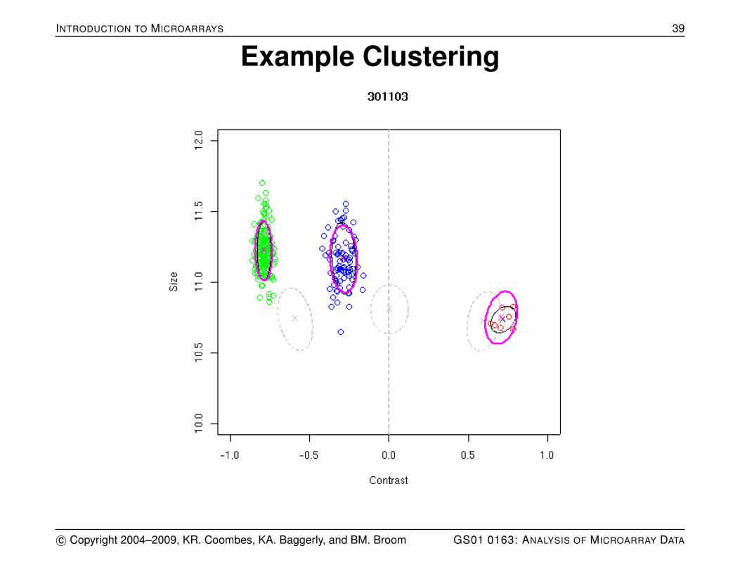
INTRODUCTION TO MICROARRAYS 39
Example Clustering
c© Copyright 2004–2009, KR. Coombes, KA. Baggerly, and BM. Broom GS01 0163: ANALYSIS OF MICROARRAY DATA

INTRODUCTION TO MICROARRAYS 40
Example Clustering
c© Copyright 2004–2009, KR. Coombes, KA. Baggerly, and BM. Broom GS01 0163: ANALYSIS OF MICROARRAY DATA

INTRODUCTION TO MICROARRAYS 41
CRLMM
Carvalho et al. developed preprocessing method thatremoves the bulk of the batch effect.
This permits the use of HapMap as training data.
Summarize probes similar to RMA.
Transform features into log ratio M and average log intensityS for both sense and antisense strands.
Use HapMap data (where available) to estimate priors ongenotype regions.
Use genotype calls that achieve at least 99% concordance,recalculate genotype centers and scales, and recomputecalls and log-likelihood ratios.
c© Copyright 2004–2009, KR. Coombes, KA. Baggerly, and BM. Broom GS01 0163: ANALYSIS OF MICROARRAY DATA

INTRODUCTION TO MICROARRAYS 42
Example on which BRLMM does poorly
c© Copyright 2004–2009, KR. Coombes, KA. Baggerly, and BM. Broom GS01 0163: ANALYSIS OF MICROARRAY DATA

INTRODUCTION TO MICROARRAYS 43
SNP Quality: CRLMM vs Birdseed
c© Copyright 2004–2009, KR. Coombes, KA. Baggerly, and BM. Broom GS01 0163: ANALYSIS OF MICROARRAY DATA
INTRODUCTION TO MICROARRAYS 44
CRLMM Availability
CRLMM is available as a Bioconductor package for R.
c© Copyright 2004–2009, KR. Coombes, KA. Baggerly, and BM. Broom GS01 0163: ANALYSIS OF MICROARRAY DATA