growth stock portfolio optimization using a multi
TRANSCRIPT
Growth Stock Portfolio Optimization Using a Multi-
Objective EA
Jeffrey Christian Alexander Goedhuys
Thesis to obtain the Master of Science Degree in
Industrial Engineering and Management
Supervisors: Prof. Rui Fuentecilla Maia Ferreira Neves
Prof. Nuno Cavaco Gomes Horta
Examination Committee
Chairperson: Prof. José Rui de Matos Figueira
Supervisor: Prof. Rui Fuentecilla Maia Ferreira Neves
Member of the Committee: Prof. João Carlos da Cruz Lourenço
June 2016
II
Abstract
This thesis presents a method to build a portfolio of growth stocks with an above index average
performance. The goal was to find good performance with a portfolio of growth stocks that are stable in
terms of price development and relatively cheap. This was done using a multi-objective genetic
evolutionary algorithm. It focusses on fundamental analysis, using quarterly data obtained from financial
statements of the companies on the S&P500 index. The use of technical analysis was minimal. The
training and simulations were done between the periods of 15-02-2012 and 13-02-2015. A short term
strategy and a long term strategy were tested. The most consistent results were obtained using a long
term multi-objective approach. Revenue growth appeared to have below average return when used as
a main indicator. The best results for a stable growth stocks portfolio were found using profit margin
growth as the main indicator. When profit margin growth was used as a main indicator, the return was
well above market average.
Keywords: genetic evolutionary algorithm, multi objective, S&P500 index, growth stocks, fundamental
analysis

III
Resumo
Nesta tese é apresentado um método de criação de uma carteira com títulos de elevado crescimento,
com um desempenho médio acima do índice. O objectivo foi encontrar um bom desempenho com uma
carteira de títulos de elevado crescimento que sejam estáveis em termos de evolução de preço e que
sejam relativamente baratos. Para tal, utilizou-se um algoritmo evolutivo genético multi-objectivo. O
algoritmo tem por base uma análise fundamental, sendo usados os dados trimestrais obtidos nas
demonstrações financeiras das empresas cotadas no índice S&P500. O uso de análise técnica foi
mínimo. O treino e simulações foram feitas entre os períodos de 15-02-2012 e 13-02-2015. Foram
testadas tanto uma estratégia a curto prazo, como uma a longo prazo. Os resultados mais consistentes
foram obtidos através de uma abordagem multi-objectivo a longo prazo. O crescimento da receita
aparentou ter um retorno abaixo da média, quando usado enquanto principal indicador. Quando o
crescimento da margem de lucro foi usado como um indicador principal, o retorno foi significativamente
acima da média do mercado.
Palavras-chave: algoritmo evolutivo genético, multi-objectivo, índice S&P500, título de elevado
crescimento, análise fundamental

IV
Acknowledgements
I would like to express my gratitude to my supervisor Rui Neves for his advice and guidance on
developing this thesis. I would also like to thank the students from the thesis discussion group for their
help and effort in the development of the scripts to acquire and organize the necessary data to do this
thesis.

V
Index
1 Introduction ....................................................................................................................................... 1
1.1 Motivation ................................................................................................................................ 1
1.2 Problem description ................................................................................................................. 2
1.3 Approach ................................................................................................................................. 2
1.4 Objectives ................................................................................................................................ 2
1.5 Structure .................................................................................................................................. 2
2 Literature Review ............................................................................................................................. 3
2.1 Growth Investing ...................................................................................................................... 3
2.2 Technical Analysis ................................................................................................................... 3
2.2.1 Dow Theory ......................................................................................................................... 4
2.2.2 Technical Indicators and Patterns ....................................................................................... 4
2.3 Fundamental Analysis ............................................................................................................. 6
2.3.1 Income Statement ................................................................................................................ 6
2.3.2 Balance Sheet ..................................................................................................................... 6
2.3.3 Cash Flow Statement .......................................................................................................... 7
2.3.4 Asset Growth Effect ............................................................................................................. 7
2.3.5 Financial Ratios ................................................................................................................... 9
2.3.6 Martin Zweig’s Approach ................................................................................................... 11
2.4 Portfolio Optimization ............................................................................................................ 12
2.4.1 Markowitz Model ................................................................................................................ 12
2.4.2 Evolutionary Computation ................................................................................................. 14
2.4.3 Algorithm Design Issues .................................................................................................... 15
2.4.4 MOEA Review ................................................................................................................... 15
2.5 Trading Systems Review ....................................................................................................... 17
2.6 Conclusion ............................................................................................................................. 18
3 System Architecture ....................................................................................................................... 20
3.1 General Investment Concept ................................................................................................. 20
3.2 Technical Analysis ................................................................................................................. 21
3.2.1 Moving Average ................................................................................................................. 21

VI
3.2.2 Stop of Losses ................................................................................................................... 22
3.3 Financial Data ........................................................................................................................ 22
3.4 Fundamental Analysis ........................................................................................................... 23
3.4.1 Revenue Growth ................................................................................................................ 23
3.4.2 Earnings Growth ................................................................................................................ 24
3.4.3 Sector ................................................................................................................................ 25
3.4.4 Profit Margin Growth .......................................................................................................... 26
3.4.5 Profit Margin (Sector Specific) ........................................................................................... 26
3.4.6 Price to Earnings Ratio ...................................................................................................... 26
3.4.7 Debt Ratio (Sector Specific) .............................................................................................. 27
3.4.8 Debt Growth ....................................................................................................................... 28
3.4.9 Revenue Growth versus Debt Growth ............................................................................... 29
3.4.10 Asset Turnover Ratio (Sector Specific) ......................................................................... 29
3.4.11 Adapted Asset Turnover Ratio Growth .......................................................................... 30
3.4.12 Return on Equity (Sector Specific) ................................................................................ 30
3.5 Evolutionary Algorithm ........................................................................................................... 31
3.6 Conclusion ............................................................................................................................. 31
4 Genetic Evolutionary Algorithm ...................................................................................................... 32
4.1 Chromosome Structure ......................................................................................................... 32
4.2 Evolutionary Process ............................................................................................................. 32
4.2.1 Individual Fitness ............................................................................................................... 33
4.2.2 Population .......................................................................................................................... 33
4.2.3 Crossover & Reproduction ................................................................................................ 33
4.2.4 Mutation ............................................................................................................................. 35
4.3 Trading Simulator Parameters ............................................................................................... 36
4.3.1 Portfolio Size ...................................................................................................................... 36
4.3.2 Minimum Score .................................................................................................................. 36
4.3.3 Stock Performance ............................................................................................................ 36
4.3.4 Cash Distribution ............................................................................................................... 37
4.4 Trading Strategy Systems ..................................................................................................... 38
4.4.1 Long Term System ............................................................................................................ 38

VII
4.4.2 Short Term System ............................................................................................................ 38
4.5 Portfolio Performance Evaluation Methods .......................................................................... 41
4.5.1 Return On Investment........................................................................................................ 41
4.5.2 Variance & Standard Deviation ......................................................................................... 41
4.5.3 Sharpe Ratio & Information Ratio ...................................................................................... 42
4.5.4 Pareto Dominance ............................................................................................................. 44
4.6 Conclusion ............................................................................................................................. 44
5 Results............................................................................................................................................ 45
5.1 Single Objective Short Term .................................................................................................. 45
5.2 Single Objective Long Term .................................................................................................. 48
5.3 Multi Objective Long Term ..................................................................................................... 49
5.4 Chromosome Composition Analysis...................................................................................... 52
5.5 Stock Selection Analysis ....................................................................................................... 52
5.6 Conclusion ............................................................................................................................. 55
6 Conclusions & Future Work............................................................................................................ 57
6.1 Conclusions ........................................................................................................................... 57
6.2 Future Work ........................................................................................................................... 57
Appendix A. Transaction List Chromosome M9

VIII
List of Figures
Figure 1. Head & Shoulder pattern Daktronics Inc. ............................................................. 5
Figure 2. Example of an efficient frontier .......................................................................... 13
Figure 3. Example typical iteration of EA with four binary decision variables ................... 15
Figure 4. Price development of CAP.PA ........................................................................... 20
Figure 5. Price Chart of GPRO .......................................................................................... 21
Figure 6. Flowchart of obtaining and organizing financial data ......................................... 23
Figure 7. Revenue and stock price of Google ................................................................... 24
Figure 8. Stock price and net income of Google .............................................................. 25
Figure 9. Debt Ratio and Price development of stock ESV ............................................... 28
Figure 10. Standard Chromosome Structure .................................................................... 32
Figure 11. Chromosome with four indicators ..................................................................... 32
Figure 12. Crossover Parent A with Parent B ................................................................... 34
Figure 13. Mutation of an individual .................................................................................. 35
Figure 14. Flowchart long term stock selection ................................................................. 39
Figure 15. Flowchart short term stock selection ................................................................ 40
Figure 16. Historical Return rates for U.S. treasury bills ................................................... 43
Figure 17. Training results plotted ..................................................................................... 50
Figure 18. Growth rates of Multi Objective Chromosomes in each trading quarter .......... 51
Figure 19. Price chart of stock RHI.................................................................................... 53
Figure 20. Price chart of stock HP ..................................................................................... 53
Figure 21. Price chart of stock URI.................................................................................... 54
Figure 22. Price history chart of TSS ................................................................................ 55
Figure 23. Price chart of the stock ROST .......................................................................... 55

IX
List of Tables
Table 1. Profitability ratios ................................................................................................... 9
Table 2. Leverage ratios ...................................................................................................... 9
Table 3. Liquidity ratios ...................................................................................................... 10
Table 4. Valuation ratios .................................................................................................... 10
Table 5. Trading systems summary .................................................................................. 19
Table 6. Revenue Growth indicator scoring method ......................................................... 23
Table 7. EPS growth indicator scoring method ................................................................. 24
Table 8. Sector indicator scoring method .......................................................................... 25
Table 9. Profit margin growth scoring method ................................................................... 26
Table 10. Scoring method for the profit margin indicator .................................................. 26
Table 11. Average S&P500 Index PER ............................................................................. 27
Table 12. Sector specific scoring for debt ratio ................................................................. 28
Table 13. Debt growth scoring method ............................................................................. 28
Table 14. Revenue vs debt growth scoring method .......................................................... 29
Table 15. Asset Turnover Ratio scoring method ............................................................... 29
Table 16. AATR scoring method ....................................................................................... 30
Table 17. Scoring for ROE indicator .................................................................................. 31
Table 18. Order of preference for combining parent chromosomes ................................. 35
Table 19. Cash Distribution over Stocks ........................................................................... 37
Table 20. Indicator number reference table ...................................................................... 45
Table 21. Training results chromosome S1 ....................................................................... 46
Table 22. Training results chromosome S2 ....................................................................... 46
Table 23. Training results chromosome S3 ....................................................................... 47
Table 24. Simulation growth rate results single objective, short term ............................... 47
Table 25. Simulation results single obj. short term............................................................ 47
Table 26. Chromosome composition, single objective long term ...................................... 48
Table 27. Simulation quarterly growth rates, single objective long term ........................... 49
Table 28. Non-dominated Solutions from Training period ................................................. 50
Table 29. Multi Objective simulation results, presented in growth rate ............................. 51

X
List of Acronyms
• AATR Adapted Asset Turnover Ratio
• AMEX American Stock Exchange
• ATR Asset Turnover Ratio
• B&H Buy and Hold
• BM Book to Market ratio
• CR Current Ratio
• DE Debt to Equity ratio
• DG Debt Growth
• DJI Dow Jones Industrial Average Index
• DR Total Debt Ratio
• DT Decision Tree
• EA Evolutionary Algorithm
• EPS Earnings Per Share
• FA Fundamental Analysis
• GA Genetic Algorithm
• IBEX35 Iberia Index 35
• IR Information Ratio
• ITR Insider Trading Ratio
• LCS Learning Classifier System
• MA Moving Average
• MOEA Multi-Objective Evolutionary Algorithm
• MVCCPO Mean Variance Cardinality Constrained Portfolio Optimization model
• NASDAQ National Association of Securities Dealers Automated Quotations
• NN Neural Network
• NOA Net Operating Assets
• NPGA Niched Pareto Genetic Algorithm
• NSGA Non-dominated Sorting Genetic Algorithm
• NYSE New York Stock Exchange
• PCR Price to Cash flow Ratio
• PER Price to Earnings Ratio
• PESA Pareto Envelope-based Selection Algorithm
• PPE Property, Plant and Equipment
• PSR Price to Sales Ratio
• QR Quick Ratio
• RDG Revenue versus Debt Growth
• RE Retained Earnings
• RG Revenue Growth

XI
• ROA Return on Assets ratio
• ROE Return on Equity ratio
• ROI Return on Investment
• RSI Relative Strength Index
• S&P500 Standard & Poor’s 500 index
• SLR Stepwise Logistic Regression
• SO Stochastic Oscillator
• SPEA Strength Pareto Evolutionary Algorithm
• SR Sharpe Ratio
• STI Straits Times Index
• TA Technical Analysis
• TF Trend Following
• XCS eXtended Classifier System

1
1 Introduction
The stock exchange market as we know it today goes back to as far as the early 1600s. It was in 1602
when the Dutch East India Company (Dutch: Vereenigde Oostindische Compagnie) was founded. It
offered stocks to fund their trading travels to South East Asia. Even though it was not the first company
to offer stocks, it was the first stock to experience lively trading. In 1611 the world’s first real stock
exchange was opened in Amsterdam, The Netherlands.
Stocks can be characterized as value or growth stocks. Studies have shown that in the past value stocks
outperform growth stocks on many occasions. In fact, in the period of 1975-1995 value stocks
outperformed growth stocks in twelve of thirteen major markets (Fama & French, 1998). At first thought
this might seem rather strange as growth stocks gain in price more rapidly than value stocks. The decline
of growth stocks can however be explained by expectation errors by traders about future earnings
prospects of these stocks. Earnings surprises are systematically more positive for value stocks (La
Porta, et al., 1997).
In Chan & Lakonishok (2004) it is suggested that investing in value stocks is not riskier than investing
in growth stocks. They found that value stocks suffered less severely than growth stocks when the
market or overall economy was performing poorly. It is more likely that the poor performance of growth
stock is caused by investor behaviour.
So how do professional investors make decisions on what stocks to invest in? In a survey conducted
with 692 fund managers in the United States, Germany, Switzerland, Italy and Thailand, it was
concluded that in each country the fund managers used three kinds of analysis. These are technical
analysis, fundamental analysis and flow analysis. For the long term, investment decisions were based
on fundamental analysis. This type of analysis dominates the forecasting for periods down to two
months. Only in the United States, technical analysis became more important in the two to six month
forecasting period. When the forecasting period was in the range of weeks (less than two months),
technical analysis was predominantly used by fund managers. In this range, the fundamental analysis
was barely used. On a forecasting period of days, the flow analysis dominates. Flow analysis is the
analysis of the trading orders. From this it can be concluded that fundamental analysis is important for
decisions on the long term, technical analysis for short term and flow analysis for the very short term
(Menkhoff, 2010). This suggests that using a combination of analysis is the best method for stock trading
in general, according to professionals. In Shynkevich (2011) investment strategies were tested using
only technical analysis for growth stocks and small capital companies. The study investigated the use
of technical analysis over the 1995-2010 period and concluded that technical analysis overall could not
provide superior returns over a simple buy-and-hold strategy.
1.1 Motivation
There is also a lot of competitors in trading. Many people are attracted to the possible riches of stock
trading, but being successful in it is not easily accomplished. It is not about just investing some cash in
stocks and hoping for the best. Learning from different approaches, there should be a method to perform
well on stock investing.

2
1.2 Problem description
The current market situation is one of high insecurity. Traders still have the crash of 2008 fresh in their
minds and the dot-com bubble is also not forgotten. Even though the markets seem to have stabilized,
negative news can cause panic among some of the traders and make them act irrationally. The stock
market is already a very dynamic environment, full of speculation, so it is the challenge to develop a
stable and successful (profitable) investment system under these conditions.
1.3 Approach
This thesis will focus on growth stocks only. Fundamental analysis will be used to select the best 10-20
companies to invest in. Ideas from Martin Zweig’s approach to stock selection will be taken, and more
fundamental indicators will be added to this, such as the asset growth effect (as a negative indicator).
The investments will be for the medium to long term, which means there will definitely not be any intraday
trading. After potential winning stocks are selected, technical analysis will anticipate on when it is time
to enter and buy the stock, and also when it is time to get out again. Fundamental analysis will also
keep track of the stocks invested in and give a signal when the financial data of a company has turned
bad and it is time to sell.
Flow indicators will not be considered, because this data is not readily available and the amount of data
would require too much computing power.
1.4 Objectives
To summarize the objectives and rules for this thesis:
• Develop a profitable automated stock trading system
• Trading is to be done on the S&P500 index
• The system must be designed to pick growth stocks for the portfolio
• The portfolio must hold stocks from 10 to 20 different companies
• Fundamental and technical analysis will be used
1.5 Structure
The remainder of the thesis is structured as follows:
• Chapter 2 describes the theories and methods used for this work
• Chapter 3 describes the architecture of the system with the indicators used and how they are
interpreted
• Chapter 4 provides detailed information on how the GA works and how performance of the
system is measured
• Chapter 5 presents and discusses the simulation results
• Chapter 6 presents the conclusion of this thesis and suggestions for future work

3
2 Literature Review
This chapter provides the basic information needed to understand how stock trading works and how a
stock trading system can be developed. It discusses technical analysis, fundamental analysis, an
approach to stock selection, evolutionary algorithms and reviews on existing multi-objective evolutionary
algorithms. At the end of this chapter a review on other trading systems developed in academic studies
can be found.
2.1 Growth Investing
Growth stocks can defined in more than one way, as it has more than a single definition. One definition
is that they are stocks of which the revenue and per-share earnings in the past have increased at well
above the rate for common stocks generally and are expected to continue to do so in the future. This
type of stocks are attractive for investors to buy and own, as long as their price is not too excessive.
This may be a problem, because growth stocks have sold at high prices (in relation to current earnings)
for a long time and at higher multiples of their average past profits over a period of time. This adds a
speculative element to investing in growth stocks (Graham, 1973).
When the expected growth fails to materialize, disappointed stockholders aggressively dump the stock,
making the price level fall to a level at which value investors become major holders of the stock. This
was the case with many technology stocks in the dot-com bubble burst in the spring of 2000 (Graham
& Dodd, 1934/2009).
2.2 Technical Analysis
Technical analysis is the study of market action, primarily through the use of chars, for the purpose of
forecasting future price trends. This analysis is based on three premises, namely (Murphy, 1999):
1. Market action discounts everything.
2. Prices move in trends.
3. History repeats itself.
The first premise ‘market action discounts everything’ indicates that a technician believes that anything
that can possibly affect the market price (fundamentals, human psychology, political influences, etc.)
has already done so. This means that the market price at any moment is indeed the real value of the
stock. This results in the technician not having to think about what can influence the market price, and
focus his study on the price movement itself is all that remains necessary (Murphy, 1999).
The second premise ‘prices move in trends’ is an essential one for technical analysis. The market price
is charted for the purpose of identifying trends in their early stage of development, so the investment
can be based on the direction the price is supposedly going to take. Trends are likely to continue to
follow their expected path until a point of reversal. The goal is to ‘ride’ this trend until it reverses (Murphy,
1999).
The third and last premise is that ‘history repeats itself’. Patterns are reflect the human psychology,
which is unlikely to change. The price patterns of the past show when a market has a bullish or bearish

4
psychology. These patterns have worked well in the past and thus are assumed to continue to do so in
the future (Murphy, 1999).
2.2.1 Dow Theory
The foundation of present day thinking in technical analysis can be traced back to the Dow Theory. The
most important concept is that of the three trends occurring in the market. Those trends are (Edwards,
et al., 2007):
1. The primary trends
This is the main direction the market is following. A trend is either an upward or downward movement.
The primary trend usually lasts for more than one year and it can maintain for up to several years. If the
primary trend is moving upwards, it is called a bullish market, if the trend is moving downwards it is
called a bearish market. This trend is the most important for long term investors.
2. The secondary trends
A smaller type of trend, interrupting the primary trend. This type of trend normally lasts from three weeks
to many months. It moves in the opposite direction of the primary trend and will take a portion of the
direction the primary trend took. The size of this portion is from about one-third up to two-thirds of what
the price has gained or lost in the primary trend.
3. The minor trends
The minor trends are only small fluctuations in the other trends, only lasting for up to three weeks. Often
they last less than six days. These minor trends are considered meaningless in the Dow theory. It is the
only trend that can be manipulated through the use of large amounts of resources.
2.2.2 Technical Indicators and Patterns
A description will follow below of the more popular technical indicators and patterns.
2.2.2.1 Moving Average
The moving average (MA) is the most well-known and widely used technical indicator. It consist of the
average price of the stock, taken over a certain number of days before the current day. The price of the
stock used to calculate the MA is usually the closing price of the days. The moving average can be over
a longer term, like 200 days down to shorter terms like 10 days (or less). Obviously the shorter term MA
is more sensitive to recent price movements.
The MA is a trend following tool, used to signal when a new trend has begun or an old trend has
reversed. It is a lagging indicator, meaning it can only follow the market trends and is only able to signal
the start or end of a new trend after it has already occurred. Shorter MAs are lagging less are following
the actual price more closely. It depends on the type of market which kind of MA (short or long) is more
useful at that given moment. Using more than one MA is useful to detect trend reversals. When a shorter
MA crosses below longer MA, it indicates a downward trend, for example. A single MA can also be used.
In this case the crossing of the MA with the price will trigger a sell signal when the price moves below
the MA and vice versa (Murphy, 1999).
A major advantage of using the MA is that it that it trades in the direction of the trend, letting profits run
and cutting the losses short. On the other hand it also shows its major flaw, as it performs poorly in

5
markets that are not subject to any trends. This can be the case in a significant amount of time, so it is
risky to rely upon solely the MA. There is an indicator called ADX, which helps to determine how much
a market is currently trending (Murphy, 1999).
2.2.2.2 Relative Strength Index
The relative strength index (RSI) is a technical indicator to determine whether a stock is overbought or
oversold. It normally uses data from the last 14 days. The formulas needed to calculate the RSI is are
as follows:
��� = 100 − ���� (1)
�� = ������ �� �� ���� ������ �� ������ �� �� ���� ������ �� ! (2)
In equation 2, the average of index points closed up and the average of index points closed down over
the last 14 days are entered. Equation 1 will then turn the formula into a number with a value between
0 and 100, which is easier to interpret (Wilder Jr., 1978).
An RSI value of over 70 indicates an overbought condition for the stock, whereas a value below 30
indicates an oversold condition (Murphy, 1999).
2.2.2.3 Head and Shoulders Pattern
The ‘head and shoulders’ pattern is a major trend reversal pattern. The price line will display three tops,
with the outer ones lower than the middle one. The tops on the outside are called the shoulders and the
middle higher top is called the head. The bottoms between the tops can be connected with a line, which
is called the neckline. The pattern, and the major trend reversal, is confirmed when the price drops below
the neckline after the final shoulder (Murphy, 1999). In figure 1, an example of the pattern is displayed.
The stock that displayed this type of behaviour is the growth stock Daktronics Inc.
Figure 1. Head & Shoulders pattern Daktronics Inc. (chart from finance.yahoo.com)

6
2.3 Fundamental Analysis
Fundamental analysis consists of analysis of a company’s financial statements, its market, industry and
macroeconomic factors. The financial statements consists of three parts:
1. Income statement
2. Balance sheet
3. Cash flow statement
Below follows a description of where relevant information for (growth) stock trading can be found and
what this information can be used for.
2.3.1 Income Statement
The income statement reflects the effect of management’s operating decisions on business performance
and the resulting accounting profit or loss for the owners of the business over a specified period of time.
It also provides performance assessment information. The income statement also shows the revenues
realized for that specific period and the costs and expenses charged against these revenues and taxes
(Helfert, 2001).
2.3.2 Balance Sheet
The balance sheet records the categories and amounts of assets employed by the company and the
offsetting liabilities incurred to lenders and owners. Balance sheets reflect the condition of a specific
moment in time, which is the date of their preparation (Helfert, 2001).
The major categories of assets are:
• Current assets (items that turn over in the normal course of business within a relatively short
period of time, such as cash, marketable securities, accounts receivable, and inventories).
• Fixed assets (such as land, mineral resources, buildings, equipment, machinery, and vehicles),
all of which are used over a longer time frame.
• Other assets, such as deposits, patents, and various intangibles.
Major sources of the funds obtained are (Helfert, 2001):
• Current liabilities, which are obligations to vendors, tax authorities, employees, and lenders due
within one year or less.
• Long-term liabilities, which are a variety of debt instruments repayable beyond one year, such
as bonds, loans and mortgages.
• Owners’ (shareholders’) equity, which represents the recorded net amount of funds contributed
by various classes of owners of the business as well as the accumulated earnings retained in
the business after payment of dividends.

7
The information from the balance sheet stated before is useful for an investor for five reasons (Graham
& Dodd, 1934/2009):
1. It shows how much capital is invested in the business.
2. It reveals the ease or stringency of the company’s financial condition, i.e., the working-capital
position.
3. It contains the details of the capitalization structure.
4. It provides an important check upon the validity of the reported earnings.
5. It supplies the basis for analysing the sources of income.
2.3.3 Cash Flow Statement
The cash flow statement captures both the current operating results and the changes they caused to
the balance sheet. It is able to provide a more dynamic picture of the changes in cash that took place
during a certain period. For this picture of change, the cash flow statement compares the beginning and
ending balance sheet for that period and also uses items of the income statement. From the statement
the following information can be found (Helfert, 2001):
• Cash generated by profitable operations or drained by unprofitable results.
• Cash impact of changes in working capital requirements.
• Commitments of cash to invest in assets or to repay liabilities.
• Raising of cash through additional borrowing or by reducing asset investments.
• Cash impact of issuance of new shares or repurchase of shares.
• Cash impact of dividends paid.
• Adjustments for accounting allocations, write-offs, and other noncash elements in the income
statement and balance sheets.
• Net impact of the period’s cash movements on the company’s cash balance.
2.3.4 Asset Growth Effect
The asset growth effect is a possible negative relation between the growth of assets on the balance
sheet of a company and its returns on stock for the period following that growth. In Cooper, Gulen and
Schill (2008), this effect is studied for non-financial companies on the U.S. stock market (NYSE, AMEX
and NASDAQ) in the period of 1963 to 2003. They calculate asset growth from both sides of the balance
sheet. On the left side they calculate total asset growth as follows:
"#$%& '(()$ *+#,$ℎ = ∆/%(ℎ + ∆/1++)2$ + ∆334 + ∆5$ℎ)+ (3)

8
Where: ∆Cash = Cash growth
∆Current = Noncash current assets growth
∆PPE = Property, Plant and Equipment growth
∆Other = Other assets growth
On the right side of the balance sheet it was calculated by the following formula:
"#$%& '(()$ *+#,$ℎ = ∆59:;%< + ∆�4 + ∆�$#=> + ∆?)<$ (4)
Where: ∆OpLiab = Operating liabilities growth
∆RE = Retained earnings growth
∆Stock = Stock financing growth
∆Debt = Debt financing growth
In short, firms with low asset growth rates earned subsequent annualized risk-adjusted returns of 9.1%
on average, while firms with high asset growth rates earned -10.4%. This is a difference of 19.5%, which
is highly significant.
The influence of the components found in equation 3 and 4 depends on the capitalization size. ∆Current
and ∆Debt has the greatest influence on the asset growth effect for small capitalization firms. This
influence shifts to ∆PPE and ∆Stock for large capitalization firms. For medium sized capitalization firms,
the influence is still mostly on ∆Current for the left side of the balance sheet and it has a more or less
equal influence for ∆Debt and ∆Stock. Growth in ∆Cash is never significant (Cooper, et al., 2008).
The causes for the asset growth effect were also investigated. The overall conclusion was that investors
over extrapolate past gains to growth.
The predictability of this effect can also be found in the net operating assets (NOA).The NOA can be
calculated with equation 5. The predictive power of NOA and its components varies across different
industries. Superior returns of hedge NOA portfolios soar when low NOA firms with asset contraction
and/or strong historical investment efficiency are considered. The asset growth effect is most likely due
to a combination of opportunistic earnings management and agency related overinvestment. The effect
is present in both good and bad states of the economy (Papanastasopoulos, et al., 2011). NOA is able
to act as a robust predictor for at least three years after it is measured. This suggests that market prices
do not fully reflect the information contained in NOA for future financial performance. This is called the
sustainability effect (Hirschleifer, et al., 2004).
A5' = ("' − /%(ℎ) − (": − �"? − :"?)(5)

9
Where: TA = Total assets
TL = Total liabilities
STD = Short term debt
LTD = Long term debt
2.3.5 Financial Ratios
Financial ratios are useful to get an idea of a company’s performance in different categories. These
ratios should be compared to those of other companies in the same market or industry. The most
important ratios will be displayed categorized in the tables found below, with the name of the ratio, the
formula used for calculation and a description of the ratio. The categories are: profitability ratios (table
1), leverage ratios (table 2), liquidity ratios (table 3) and valuation ratios (table 4).
Name Formula Description
Return on Equity
(ROE) �54 = A)$ �2=#C)'D)+%E) �ℎ%+)ℎ#&F)+( 4G1;$H (6)
Shows how much
profit a company is
able to generate with
the money
shareholders invested.
Return on Assets
(ROA) �5' = A)$ �2=#C)"#$%& '(()$( (7)
Shows earnings
generated by a
company from its total
assets.
Net Profit Margin A)$ 3+#K;$ L%+E;2 = A)$ 3+#K;$A)$ �%&)( (8) Shows how much a
company keeps in
earnings from every
dollar made in sales.
Table 1. Profitability Ratios
Name Formula Description
Total Deb ratio (DR) ?� = "#$%& :;%<;&;$;)("#$%& '(()$( (9) Shows how much of
the company’s assets
are financed through
debt.
Debt to Equity ratio
(DE) ?4 = "#$%& :;%<;&;$;)(�ℎ%+)ℎ#&F)+( 4G1;$H (10)
Shows if the company
is currently more
financed through debt
or by shareholders.
Table 2. Leverage Ratios

10
Name Formula Description
Current
ratio (CR) /� = /1++)2$ '(()$(/1++)2$ :;%<;&;$;)( (11)
Shows the
ability of a
company to
pay its short
term
obligations. A
value below 1
means it
cannot fulfil all.
Quick ratio
(QR) O� = /%(ℎ & �ℎ#+$ $)+C �2D)($C)2$( + '==#12$( �)=);D%<&)/1++)2$ :;%<;&;$;)( (12)
A more
conservative
version of the
CR. It only
takes into
account the
assets with the
most liquidity.
Table 3. Liquidity Ratios
Name Formula Description
Earnings per
Share (EPS) 43� = A)$ �2=#C) − ?;D;F)2F( #2 3+)K)+)F �$#=>('D)+%E) 51$($%2F;2E �ℎ%+)( (13)
Shows the income for
each outstanding
common share.
Price to
Earnings ratio
(PER)
34� = L%+>)$ R%&1) 9)+ �ℎ%+)43� (14) Shows how much a
shareholder is willing
to pay for future
expected earnings.
Price to Sales
ratio (PSR) 3�� = L%+>)$ R%&1) 9)+ �ℎ%+)�%&)( 9)+ �ℎ%+) (15)
Show how much a
share is worth for
each dollar made on
sales.
Price to Cash
Flow ratio
(PCR)
3/� = L%+>)$ R%&1) 9)+ �ℎ%+)/%(ℎ S&#, 9)+ �ℎ%+) (16) Shows the price in
relation to a
company’s cash flow.
Book to
Market ratio
(BM)
TL = T##> R%&1) #K $ℎ) =#C9%2HL%+>)$ R%&1) #K $ℎ) =#C9%2H (17) Compares the book
value of the company
to its market value.
Table 4. Valuation Ratios

11
2.3.6 Martin Zweig’s Approach
Martin Zweig developed an investment methodology suited for growth stocks. He described this method
in his book ‘Winning on Wall street’ (1986). It focuses on picking the stocks with the best future growth
potential. The major points of this stock picking methodology will described below.
• Look for growth in sales and EPS
The first step is to look for companies that have growth in both sales and EPS. For this it is best to
compare quarterly figures from consecutive years against each other. This will eliminate seasonal sales
variables. Growth stability is also important, as it is an indicator of decent accounting. If the growth is at
a steady rate, it is less likely the numbers are being manipulated in the income statements.
• Stock must have a reasonable PER
Low PER companies outperform high PER companies in the long term. Companies with a high PER
should be avoided. It is an indication of higher risk, as the room for error decreases. When the company’s
expected growth fails to materialize, it will cause the stock price to drop significantly. Companies on the
very low end of the PER, may be in financial trouble, so these are best avoided too, or require a more
thorough study of their balance sheet or other data for negative indications. It is best to find stocks with
a PER close the market average. As an example, if the market average is 10 and there is a stock with
good growth figures that has a PER of 12, it would be considered a bargain. 16 and 17 would be on the
high end and only be worth it if the company shows a high enough growth rate and has a significant
competitive advantage. To make some sense out of what might be a reasonable PER, the earnings
trend of the past several years should be studied (Zweig, 1986).
• Relative strength of price action
The relative price gain of the stock should be compared to the market average (in this case that of
S&P500). If a stock is really good, it should be outperforming the market. Also, in a very strong market,
the best growth pattern is that of a stepladder going up. This means that there is a clear upward trend,
with higher highs and higher lows. It will have small downward moves, but as long as they do not go
below a previous low, it is acceptable. The best buying spots would in this case be those short term
bottoms of 5% to 10% (leverage).
• Track insider trading
Insider trading is the trading of stocks done by people who have access to information about company
they traded the stocks from, which is not publicly available. This could be officers, directors or
employees. In the United States of America, people who perform an insider trade, are required to report
this trade. This information is publicly accessible.
The importance of insider trading is that when they are selling the stock heavily, something must be
wrong with the company. If there is only very little insider trading, this can be ignored. This also works
the other way around, meaning that if insiders are starting to buy the stock more frequently it is a positive
indication.

12
Study shows that from insider trades, those made directors and officers do have predictive power for
future returns. If an outsider was able to mimic their behaviour, he would make positive trading returns.
Director actions have predictive power for firms of all sizes, while officers’ actions only have predictive
power for small firms. Trading actions from directors and those of officers (although to a lesser extent)
have significant influence on the trades of other insiders (Tavakoli, et al., 2011).
• Debt should be considered
Although not outlined as a major point, it is considered important to evaluate the level of debt of a
company. If a company has high levels of debt, it may get in trouble when it has to pay off its interest
for the year, which can greatly cut into the earnings of a company. Debt should be used as a negative
predictor for stock selection.
2.4 Portfolio Optimization
In finance, a portfolio is a collection of assets held by an institution or a private individual. The portfolio
seeks an optimal way to distribute a given budget on a set of available assets (stocks). The problem
usually has two criteria set against each other: the expected return (mean profit) and the risk. The return
is an objective function that needs to be maximized, while the risk needs to be minimized. This makes
it a multi-objective optimization problem. Risk can be measured as the variance of the portfolio return.
Mean-variance optimization is a popular approach to portfolio selection problems (Branke, et al., 2008).
2.4.1 Markowitz Model
The mean-variance optimization model was introduced by Markowitz in 1952. The basics of this model
are shown below (Markowitz, 1952):
The variance equals:
R(�) = U U %V%WXVWY
WZ�Y
VZ� (18)
With the total portfolio return being:
� = U �V%V (19)
Where: V = Variance
R = Return
Ri = Expected return on asset i
σij = covariance between asset i and asset j
ai = weight for asset i
aj = weight for asset j
For the weights: ∑ %VYVZ� = 1, 0 ≤ ai ≤ 1, i = 1, ... , n

13
Using different values for R, the results can be projected into a graph. This graph will show the efficient
(non-dominated) portfolios with the efficient frontier, also called the Pareto front. IN figure 2, an example
of such a graph is shown, with the return (or mean) projected on the Y-axis and the risk (or variance)
projected on the X-axis. Depending on the risk aversion of the decision maker, a suitable portfolio can
be selected through this graph. This is because the risk is spread over several stocks, also called
diversification (Chang, et al., 2000).
Figure 2. Example of an efficient frontier (Chang, et al., 2000)
Throughout the years the basic Markowitz model has been expanded with constraints to reflect the
decision making process of fund managers in the real world. One of these expanded models has
something called the cardinality constraint, which restricts the number of assets in the portfolio and the
amount of each asset as part of the portfolio. This particular expanded model is called the ‘mean-
variance cardinality constrained portfolio optimization model’ (MVCCPO).Building on the previously
stated basic model, it is formulated as (Chang, et al., 2000) (Anagnostopoulos & Mamanis, 2011):
C;2;C;]) R(�) = U U %V%WXVWY
WZ�Y
VZ� (18)
C%^;C;]) � = U �V%VY
VZ� (19)
Subject to:
U %VY
VZ�= 1 (20)

14
ɛV`V ≤ %V ≤ bV`V , i = 1, ... , n (21)
U `VY
VZ�= c (22)
`V ∈ e0,1f , ; = 1, … , 2 (23)
Equation 21 limits the amount invested in a stock i, with a lower limit of ɛi and an upper limit of δi. Equation
22 has K being the value of maximum stocks allowed to put in portfolio. Equation 23 sets if stock i is
held or not, using a binary.
2.4.2 Evolutionary Computation
The optimal solutions inside the decision space (Pareto set) can be hard to generate due to the
complexity of the problem (it can be infeasible) and the computing resources required. As a work around,
stochastic search strategies can be used. These do not always find the optimal solutions, but will try to
approximate them as closely as possible. One of these strategies is using an evolutionary algorithm
(EA). They are based on the idea of natural evolution. Any possible solution is called an ‘individual’ and
a set of solution candidates is called the ‘population’. The quality of each individual in the current
population is referred to as their ‘fitness’. The fitness is measured with a scalar value (Zitzler, et al.,
2004).
2.4.2.1 Chromosomes
Individuals are represented in chromosomes. On these chromosomes the indicators (such as the
fundamental indicators) are encoded as a gene.
2.4.2.2 Mating Pool
The mating pool holds the individuals selected from the population which will be used to create a new
generation. The mating selection is based on sampling from the population. From this sample the ones
with best fitness will be selected to join the mating pool. This selection process can be done in more
than one way. One example is tournament selection, which selects two random individuals from the
population and picks the one with the best fitness value to join the mating pool while eliminating the
other. The main difference between MOEAs is the way they assign a fitness value to individuals
(Anagnostopoulos & Mamanis, 2011) (Zitzler, et al., 2004).
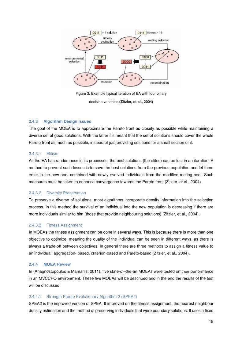
To complete the picture of how a single iteration works in EA, see figure 3. After recombination of two
individuals a mutation can be added to add variation. The environmental selection is the final step to a
new population. It can pick individuals from the old population and the modified mating pool.
15
Figure 3. Example typical iteration of EA with four binary
decision variables (Zitzler, et al., 2004)
2.4.3 Algorithm Design Issues
The goal of the MOEA is to approximate the Pareto front as closely as possible while maintaining a
diverse set of good solutions. With the latter it’s meant that the set of solutions should cover the whole
Pareto front as much as possible, instead of just providing solutions for a small section of it.
2.4.3.1 Elitism
As the EA has randomness in its processes, the best solutions (the elites) can be lost in an iteration. A
method to prevent such losses is to save the best solutions from the previous population and let them
enter in the new one, combined with newly evolved individuals from the modified mating pool. Such
measures must be taken to enhance convergence towards the Pareto front (Zitzler, et al., 2004).
2.4.3.2 Diversity Preservation
To preserve a diverse of solutions, most algorithms incorporate density information into the selection
process. In this method the survival of an individual into the new population is decreasing if there are
more individuals similar to him (those that provide neighbouring solutions) (Zitzler, et al., 2004).
2.4.3.3 Fitness Assignment
In MOEAs the fitness assignment can be done in several ways. This is because there is more than one
objective to optimize, meaning the quality of the individual can be seen in different ways, as there is
always a trade-off between objectives. In general there are three methods to assign a fitness value to
an individual: aggregation- based, criterion-based and Pareto-based (Zitzler, et al., 2004).
2.4.4 MOEA Review
In (Anagnostopoulos & Mamanis, 2011), five state-of–the-art MOEAs were tested on their performance
in an MVCCPO environment. These five MOEAs will be described and in the end the results of the test
will be discussed.
2.4.4.1 Strength Pareto Evolutionary Algorithm 2 (SPEA2)
SPEA2 is the improved version of SPEA. It improved on the fitness assignment, the nearest neighbour
density estimation and the method of preserving individuals that were boundary solutions. It uses a fixed

16
archive size, filling any open spots with dominated individuals, or deleting excess non-dominated
individuals based on the density information. The fitness value is assigned so that the best solutions
have the minimum value (0) (Anagnostopoulos & Mamanis, 2011) (Zitzler, et al., 2004).
2.4.4.2 Non-dominated Sorting Genetic Algorithm II (NSGA-II)
An improved version of NSGA, which main points of criticism were: the lack of elitism, high computational
complexity of non-dominated sorting and the need of specifying a sharing-parameter to ensure diversity
of solutions. The non-dominating sorting has been made faster in the new version requiring O(MN2)
computations instead of O(MN3) previously. Best individuals are picked from the archive and population.
If solutions with same fitness do not all fit into the archive, the ones with a lower density have priority
(Deb, et al., 2002) (Anagnostopoulos & Mamanis, 2011).
2.4.4.3 Niched Pareto Genetic Algorithm 2 (NPGA2)
Also an improved version of a predecessor. It uses tournament selection to select individuals for the
mating pool. The winner of each sample is determined by Pareto rank. Diversity preservation is done
through a niche-count, with a niche radius to be set by the user of the algorithm (Erickson, et al., 2001)
(Anagnostopoulos & Mamanis, 2011).
2.4.4.4 Pareto Envelope-based Selection Algorithm (PESA)
Non-dominated individuals of the population are send to the archive. With each iteration this step is
repeated, sending new non-dominated individuals to the archive until a termination criterion has been
reached. If the archive gets too full, the one with worst fitness gets eliminated. Parent selection is based
on density, to preserve diversity (Corne, et al., 2000).
2.4.4.5 e-MOEA
This algorithm uses a similar method for selection, focussing on non-dominated individuals. Users
specify an e-value. This value is the distance within which no other solutions are allowed. If a new non-
dominated individual is entered into the archive, and dominates another individual in the archive within
e distance, the dominated one is eliminated (Hanne, 2007) (Anagnostopoulos & Mamanis, 2011).
2.4.4.6 Evaluation Results
Five test problems were used. SPEA2 won four out of these five tests, making it superior to the other
MOEAs. The second best performers were NSGA-II and e-MOEA, having similar performance results.
e-MOEA is a lot faster than NSGA-II though, requiring only half the run time. SPEA2 requires the
greatest amount of computing power of all algorithms, whereas PESA is the quickest (Anagnostopoulos
& Mamanis, 2011).

17
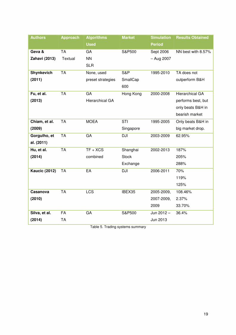
2.5 Trading Systems Review
There are numerous papers on developed trading systems. Some with the goal to maximize profit, while
others study the effect of a particular approach to stock market trading. Several of these trading systems
will be shortly described below, with the results obtained. A general overview can be found in table 5.
In Geva & Zahavi (2013) the effectiveness of using textual news is studied. Decisions of buying stock
are only based on market data and different levels of textual news. Each level added using an extra
textual indicator. These indicators were: simple news count, categorized news, sentiment of news and
finally calibrated sentiment of news (more elaborate sentiment). Textual news data was extracted from
the Reuters3000 service. All trading was intraday, having decision points of buying stock every five
minutes and always selling that stock exactly one hour later. The best result was obtained using the
most complete level of textual news combined with general market data, which had a profit of 8.57%,
using a Neural Network (NN) algorithm. They also tested it using a Genetic Algorithm (GA) and a
Stepwise Logistic Regression (SLR) algorithm. The market was S&P500 over the period of September
2006 till August 2007.
Already mentioned in the introduction, Shynkevich (2011) studied if TA on its own would be able to
outperform a B&H strategy over the period of 1995-2010. The study was aimed at growth stocks and
small cap stocks. These came from different sectors on the S&P SmallCap 600 index. The general
conclusion is that TA does not outperform a buy-and-hold strategy.
In Fu, et al. (2013) they also use just TA. They however weight them using a traditional GA and a
Hierarchical GA (best fitness of pool of eliminated individuals replaces worst fitness in winners pool).
The study was on the Hong Kong index over the period 2000-2008, which had both a bearish and bullish
market period. They found that TA optimized through a GA does perform profitable in both market
periods, but gets outperformed by B&H strategies in a bullish market. The Hierarchical GA performs
better than the traditional GA, but takes longer to reach convergence towards the Pareto front.
Perhaps not adding to the conclusions already found in previously mentioned papers, in Chiam, et al.
(2009) a trading system using combinations of only three technical indicators was studied. These
indicators were MA, RSI and SO (Stochastic Oscillator). They were optimized using an MOEA and
tested on the Straits Times Index in Singapore. It could only beat buy-and-hold in a period the market
made a huge drop, while in a period where B&H achieved 76.60% return, their system only achieved
20.18%. The study was over the period of 1995-2005.
Staying on the topic of using a GA to optimize a TA system, another such a study was done on the Dow
Jones Industrial Average Index (DJI) by Gorgulho, et al. (2011). Their system was tested over the period
of 2003-2009 against the B&H strategy and a random strategy. The best GA achieved a ROI of 62.95%
over this period, with 88.46% profitable positions. They conclude to have outperformed the B&H and
random strategy with their system over this time span. Although this is true, it was mainly the crash that
caused a fall-back of the B&H strategy, which was slightly outperforming the average GA until the market
crash. The GA performed reliably during this period.
In Hu, et al. (2014) a trend following (TF) algorithm is used. They use a hybrid for long and short term
trend following, called e-Trend. This is a TF combined with eXtended Classifier Systems (XCS). XCS is
18
in turn a GA with reinforced learning. Using the e-Trend algorithm on the various parts of the Shanghai
Stock Exchange in 2002-2013, they achieve superior results compared to B&H, a Decision Tree (DT)
algorithm and a NN algorithm. The accumulative returns were: 187%, 205% and 288%.
In Kaucic (2012), a TA system is used with an EA, which acts according to a preset investment strategy
aimed at seeking overbought and oversold stock. The three formed portfolios achieved a return of 70%,
119% and 125%, during the period of 2006-2011 on the DJI. The system did however perform below
market average during the crisis, but recovered faster.
Casanova (2010) developed a system based on a Learning Classifier System (LCS), Pittsburgh-style.
LCS is based on reinforced learning. The indicators are all from TA and it has two variants with a stop
command, selling a stock if it loses 2% or 4% in value. The simulation periods were 2005-2009, 2007-
2009 and the year 2009 on its own. These gave a total return of 108.46%, 2.37% and 33.70%
respectively. The first period result was achieved with a 2% stop command and the other two with a 4%
stop command. The stocks were traded on the Spanish IBEX35.
The final trading system reviewed is that of Silva, et al. (2014). It uses a number of fundamental
indicators to select the best stocks to invest in. These indicators were weighted with a EA. The best
stocks will be selected to enter the portfolio. Then technical trading rules will decide on market entry and
exit. The best chromosome had a return of 36.4% while the market average (S&P500) had a return of
25.55%. The period of the result was June 2012 to June 2013.
2.6 Conclusion
This chapter provided the basic knowledge needed to set up a trading system. It explained what growth
stock are and presented an approach to find such stocks. The idea behind technical analysis was
presented together with some basic trend reversal indicators. Many fundamental indicators such as the
ratios were presented and in the next chapter it will be discussed how a number of these will be
incorporated into the system.
The basic information about MOEA is used in portfolio optimization was given. At the end of the chapter
numerous previous researches on trading systems were discussed. It showed what algorithms they
used and what their main approach was. It also presented the results obtained by them.
19
Authors Approach Algorithms
Used
Market Simulation
Period
Results Obtained
Geva &
Zahavi (2013)
TA
Textual
GA
NN
SLR
S&P500 Sept 2006
– Aug 2007
NN best with 8.57%
Shynkevich
(2011)
TA None, used
preset strategies
S&P
SmallCap
600
1995-2010 TA does not
outperform B&H
Fu, et al.
(2013)
TA GA
Hierarchical GA
Hong Kong 2000-2008 Hierarchical GA
performs best, but
only beats B&H in
bearish market
Chiam, et al.
(2009)
TA MOEA STI
Singapore
1995-2005 Only beats B&H in
big market drop.
Gorgulho, et
al. (2011)
TA GA DJI 2003-2009 62.95%
Hu, et al.
(2014)
TA TF + XCS
combined
Shanghai
Stock
Exchange
2002-2013 187%
205%
288%
Kaucic (2012) TA EA DJI 2006-2011 70%
119%
125%
Casanova
(2010)
TA LCS IBEX35 2005-2009,
2007-2009,
2009
108.46%
2.37%
33.70%
Silva, et al.
(2014)
FA
TA
GA S&P500 Jun 2012 –
Jun 2013
36.4%
Table 5. Trading systems summary

20
3 System Architecture
This chapter starts by explaining the general investment concept, goals and strategies. After that it will
explain which technical and fundamental indicators are used and how they are used to attempt to
achieve the goal. These indicators require financial data to be calculated. One section in this chapter
will show how the required financial data was obtained. At the end of the chapter it will explain how the
EA will be used with the indicators.
3.1 General Investment Concept
Before discussing all the indicators it is important to understand the goals of the investment. The general
goal is to achieve an above index average profit with a low risk of losing money on the investment. The
growth stocks that are looked for to achieve this goal should be relatively cheap (no high PER) and be
subject to a stable above index average growth rate.
A good example of such a growth stock is the stock of Cap Gemini (CAP.PA) on the French CAC40
(Cotation Assistée en Continu) index. The development of this stock can be found in figure 4. At the
moment of writing this stock has a PER of around 21, which means it is not an expensive stock.
Figure 4. Price development of CAP.PA (source: finance.yahoo.com)
There is also an example to demonstrate what can happen to stocks that grow too quickly and become
a risky investment, namely GoPro (GPRO). This company could not keep up with the expected growth
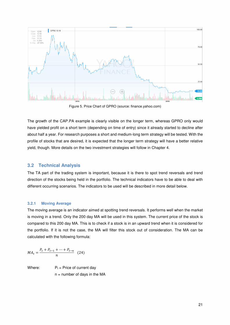
and the price fell deeply after an initial growth spurt. The price development of GPRO can be found in
figure 5. Even at its current day low, the PER is over 50, which makes it a relatively expensive stock.
21
Figure 5. Price Chart of GPRO (source: finance.yahoo.com)
The growth of the CAP.PA example is clearly visible on the longer term, whereas GPRO only would
have yielded profit on a short term (depending on time of entry) since it already started to decline after
about half a year. For research purposes a short and medium-long term strategy will be tested. With the
profile of stocks that are desired, it is expected that the longer term strategy will have a better relative
yield, though. More details on the two investment strategies will follow in Chapter 4.
3.2 Technical Analysis
The TA part of the trading system is important, because it is there to spot trend reversals and trend
direction of the stocks being held in the portfolio. The technical indicators have to be able to deal with
different occurring scenarios. The indicators to be used will be described in more detail below.
3.2.1 Moving Average
The moving average is an indicator aimed at spotting trend reversals. It performs well when the market
is moving in a trend. Only the 200 day MA will be used in this system. The current price of the stock is
compared to this 200 day MA. This is to check if a stock is in an upward trend when it is considered for
the portfolio. If it is not the case, the MA will filter this stock out of consideration. The MA can be
calculated with the following formula:
L'h = 3h + 3hi� + ⋯ + 3hiY2 (24)
Where: Pt = Price of current day
n = number of days in the MA

22
3.2.2 Stop of Losses
The system must be protected by a trading rule against heavy sudden losses. The maximum allowable
limit of loss depends on the investment strategy (short term, medium term or long turn). If the loss
exceeds the limit, the system must sell the stock to protect it from even greater losses. The limit of the
stop-loss trigger can be linked to the entire index movement. This is to not lose large amounts of money
on very short sudden drops in the macro-economic environment caused by, for example, a terrorist
attack. Such a dynamic stop-loss trigger is only needed when the value of the maximum allowable loss
is low. Also, it can only be dynamic when the index is on a downward trend.
The basic formula for the stop-loss trigger can be found in equation 25. The dynamic formula can be
found in equation 26.
�)&& �$#=>, ;K: 3�h��l �m���Yh < (1 − ($#9&#(() ∗ 3�h��l VYVhV�� (25)
;K: 3pY��q �m���Yh < 3pY��q VYVhV�� �)&& ($#=>, ;K: 3�h��l �m���Yh < r3VY��q �m���Yh3VY��q VYVhV�� − ($#9&#((s ∗ 3�h��l VYVhV��(26)
Where: Pstock initial = Price of stock when added to portfolio
Pstock current = Price of stock at the current day
Pindex initial = Price of index (S&P500) at start of trading quarter
Pindex current = Price of index (S&P500) at the current day
Stoploss = maximum allowable loss
3.3 Financial Data
For the various fundamental indicators discussed in chapter 2, financial data of all companies in the
S&P500 index is required. This data was extracted from different sources. The data on stock prices was
taken from the Yahoo Finance website. The data used for fundamental analysis, such as the earnings
reports and balance sheets, were extracted from the SEC (U.S. Securities and Exchange Commission)
website. Various scripts were used to extract and organize the data. An overview of data collection can
be found in figure 6.

23
Figure 6. Flowchart of obtaining and organizing financial data
3.4 Fundamental Analysis
After extraction of the financial data, the financial indicators can be set. The data has to be transformed
into ratios for each company, to allow comparison between companies. The following indicators will be
used in the trading system. At the end of each indicator’s section a table can be found with the scoring
system for that particular indicator. The scores are used to assess a company’s financial state according
to the indicator. The scores are based on the spread of data used for the indicator and on what can be
considered a positive and negative score on the used scale (a negative income cannot receive a positive
score, for example).
3.4.1 Revenue Growth
As described in the section about the Zweig Approach, the first things to look for a growth in sales and
growth in earnings. This growth should be quite stable or be increasing ( no major fluctuations). The
relation between revenue and stock price can be seen in figure 7. To avoid misreading seasonal sales
as a fluctuation, the growth should be compared from the quarterly reports against the reports from the
same quarter in previous years. The revenue growth (RG) can be calculated as follows:
�)D)21)*+#,$ℎ = �)D)21)h − �)D)21)hi��)D)21)hi� (27)
Revenue Growth
Score -2 -1 0 1 2 1
Indicator Range < -0.05 ≥ -0.05 ≥ 0 ≥ 0.05 ≥ 0.1 ≥ 0.15
Table 6. Revenue Growth indicator scoring method

24
Figure 7. Revenue and stock price of Google
3.4.2 Earnings Growth
The growth in earnings is very important to shareholders, especially in growth stocks. If the expected
growth fails to materialize, the stock can get dumped. With growth stocks this happens more quickly,
because in general the prices are higher and thus a shareholder is more likely to be disappointed. To
evaluate the earnings growth, the EPS of several periods are compared. Once again it is better to
compare quarterly reports with each other. The growth in EPS has nearly the same formulation as the
revenue growth:
43� *+#,$ℎ = 43�h − 43�hi�43�hi� (28)
The relation between stock price and earnings can be seen in figure 8 below. The scoring method for
EPS growth can be found in table 7.
EPS Growth
Score -2 -1 0 1 2 1
Indicator
Range
< -0.05 ≥ -0.05 ≥ 0 ≥ 0.05 ≥ 0.1 ≥ 0.15
Table 7. EPS growth indicator scoring method

25
Figure 8. Stock price and net income of Google
3.4.3 Sector
Companies in the S&P 500 index are categorized into sectors. These are Consumer Discretionary,
Consumer Staples, Energy, Financials, Health Care, Industrials, Information Technology, Materials,
Telecommunication Services and Utilities. Stocks in certain sectors can be more sensitive to macro-
economic changes than those of other sectors. For example, the average forward revenue of companies
in the sector Health Care were barely affected by the financial crisis around 2008, while the average
forward revenue of companies in the sector Materials went down considerably (Yardeni & Abbott, 2015).
The sector can thus give an indication of the risk involved in investing into a stock of this sector. The
method of scoring this indicator can be found in table 8.
Sector Score
Health Care 2
Consumer Discretionary 1
Information Technology 1
Consumer Staples 0
Industrials 0
Energy 0
Materials -1
Utilities -2
Financials -2
Telecommunications
Services
-2
Table 8. Sector indicator scoring method

26
3.4.4 Profit Margin Growth
This indicator should help determine how well the costs the company makes are controlled. It gives a
clear relationship between the revenue and the earnings. Growth in revenue and earnings is desired
and if this ratio is also growing, it means the company is also increasing its cost effectiveness.
Scoring for this indicator can be found in table 9. The general equation for calculating the profit margin
can be found in equation 29.
Profit Margin Growth
Score -2 -1 0 1 2
Indicator Range < -0.05 ≥ -0.05 ≥ 0 ≥ 0.05 ≥ 0.1
Table 9. Profit margin growth scoring method
3+#K;$ L%+E;2 = A)$ �2=#C)�)D)21) (29)
3.4.5 Profit Margin (Sector Specific)
Another way to review the cost effectiveness of a company is to compare its profit margin to those of
other companies within the same sector. The sector specific scoring method can be found in table 10.
Profit Margin Score
-2 -1 0 1 2
Health Care < 0.05 ≥ 0.05 ≥ 0.1 ≥ 0.2 ≥ 0.3
Consumer Discretionary < -0.1 ≥ -0.1 ≥ 0.1 ≥ 0.15 ≥ 0.3
Information Technology < 0.1 ≥ 0.1 ≥ 0.2 ≥ 0.3 ≥ 0.4
Consumer Staples < 0.07 ≥ 0.07 ≥ 0.15 ≥ 0.3 ≥ 0.4
Industrials < 0.1 ≥ 0.1 ≥ 0.15 ≥ 0.2 ≥ 0.25
Energy < 0.1 ≥ 0.1 ≥ 0.15 ≥ 0.2 ≥ 0.3
Materials < 0.05 ≥ 0.05 ≥ 0.1 ≥ 0.15 ≥ 0.2
Utilities < 0.05 ≥ 0.05 ≥ 0.1 ≥ 0.15 ≥ 0.2
Financials < 0.1 ≥ 0.1 ≥ 0.2 ≥ 0.3 ≥ 0.4
Telecommunications
Services
< 0.04 ≥ 0.04 ≥ 0.08 ≥ 0.12 ≥ 0.16
Table 10. Scoring method for the profit margin indicator
3.4.6 Price to Earnings Ratio
This ratio shows how much growth is expected from shareholders, because they pay a price higher than
the earnings per share. Although growth stocks are considered to have a high PER, if it is too high the
risk on the share will increase, since it will get dumped more quickly with a bad earnings report. It is not
easy to just set a limit on how high or low the PER can be. The stock’s average of the preceding year
(last four quarters) will be used to calculate the current PER. To stay within a certain boundary, a PER

27
no higher or lower than 1.4 times the market average will be applied. The value to which the filter is set,
is determined by the average S&P500 PER on January 1st of the trading period’s year. The average
ratios of the years used can be found in table 11 below. The PER can be calculated with equation 30.
34� = /1++)2$ �$#=> 3+;=)'221%& 43� (30)
Date PER Value
01-01-2015 20.02
01-01-2014 18.15
01-01-2013 17.03
01-01-2012 14.87
Table 11. Average S&P500 Index PER (Shiller, 2006)
3.4.7 Debt Ratio (Sector Specific)
The DR is an indicator of risk for bankruptcy of a company. If this ratio increases, the risk of investing in
that company is increasing too. An example of the influence of an increasing debt ratio on the stock’s
price can be seen in figure 9.
It is also important to remember that debt comes with the payments of interest, which will cut into the
earnings of a company. High debt will therefore reduce the potential earnings of the company, which in
turn can cause the price of the stock to go down. Preferably a company with no debt will be picked, but
growth companies may need to take up loans to finance the company’s growth. This ratio is only
important when the number becomes excessively high.
The scoring method for the sector specific debt ratio can be found in table 12. The formula to calculate
the debt ratio as used for the indicator can be found in equation 31.
?)<$ �%$;# = :#2E ")+C ?)<$"#$%& '(()$( (31)

28
Figure 9. Debt Ratio and Price development of stock ESV
Debt Ratio Score
-2 -1 0 1 2
Health Care ≥ 0.25 ≤ 0.25 ≤ 0.2 ≤ 0.15 ≤ 0.1
Consumer Discretionary ≥ 0.4 ≤ 0.4 ≤ 0.3 ≤ 0.2 ≤ 0.1
Information Technology ≥ 0.28 ≤ 0.28 ≤ 0.21 ≤ 0.14 ≤ 0.07
Consumer Staples ≥ 0.4 ≤ 0.4 ≤ 0.3 ≤ 0.2 ≤ 0.1
Industrials ≥ 0.25 ≤ 0.25 ≤ 0.2 ≤ 0.15 ≤ 0.1
Energy ≥ 0.25 ≤ 0.25 ≤ 0.2 ≤ 0.15 ≤ 0.1
Materials ≥ 0.22 ≤ 0.22 ≤ 0.17 ≤ 0.12 ≤ 0.07
Utilities ≥ 0.23 ≤ 0.23 ≤ 0.17 ≤ 0.11 ≤ 0.05
Financials ≥ 0.2 ≤ 0.2 ≤ 0.15 ≤ 0.1 ≤ 0.05
Telecommunications
Services
≥ 0.25 ≤ 0.25 ≤ 0.2 ≤ 0.15 ≤ 0.1
Table 12. Sector specific scoring for debt ratio
3.4.8 Debt Growth
Like the DR, the growth of debt can be considered to see how risky it is to invest into a company. By
reviewing the growth of debt it can be seen whether a company is becoming more or less reliant on
investments from outside and thus able to support itself independently. The scoring method can be
found in table 13.
Debt Growth
Score -2 -1 0 1 2
Indicator Range ≥ 0.05 ≤ 0.05 ≤ 0 ≤ -0.05 ≤ -0.1
Table 13. Debt growth scoring method

29
3.4.9 Revenue Growth versus Debt Growth
As explained in the last paragraph, growth companies can have debt when they’re still investing. It is
more important that the cash from debt is invested in such a way that it helps to generate revenue.
Therefore the RG can be set out against the debt growth (DG). It would not be good if the debt keeps
increasing but the revenue is not. The indicator for revenue versus debt growth (RDG) will be the
following:
�?* = �* − ?* (32)
When the number is negative, it indicates the debt grows at a higher rate than the revenue. This is a
signal for bad investments. If the RDG is positive, revenue grows at a higher rate. In case DG is negative
(debt became smaller), it should add to the RDG, which is a good signal.
The scoring method for the revenue vs debt indicator can be found in table 14.
Revenue vs Debt
Growth
Score -2 -1 0 1 2
Indicator Range < -0.1 ≥ -0.1 ≥ 0 ≥ 0.1 ≥ 0.2
Table 14. Revenue vs debt growth scoring method
3.4.10 Asset Turnover Ratio (Sector Specific)
The general asset turnover ratio (ATR) is useful to see how well a company uses its assets. A higher
ratio is better. The reason revenue is chosen instead of earnings to calculate the ratio, is because debt
can influence the earnings, making the revenue more stable as an indicator. The ATR can be calculated
using equation 33.
The scoring method for this ratio can be found below in table 15.
Asset Turnover Ratio Score
-2 -1 0 1 2
Health Care < 0.1 ≥ 0.1 ≥ 0.15 ≥ 0.2 ≥ 0.25
Consumer Discretionary < 0.1 ≥ 0.1 ≥ 0.2 ≥ 0.3 ≥ 0.5
Information Technology < 0.05 ≥ 0.05 ≥ 0.1 ≥ 0.15 ≥ 0.2
Consumer Staples < 0.1 ≥ 0.1 ≥ 0.2 ≥ 0.3 ≥ 0.4
Industrials < 0.07 ≥ 0.07 ≥ 0.14 ≥ 0.21 ≥ 0.28
Energy < 0.07 ≥ 0.07 ≥ 0.12 ≥ 0.2 ≥ 0.3
Materials < 0.07 ≥ 0.07 ≥ 0.14 ≥ 0.21 ≥ 0.28
Utilities < 0.06 ≥ 0.06 ≥ 0.12 ≥ 0.18 ≥ 0.24
Financials < 0.1 ≥ 0.1 ≥ 0.15 ≥ 0.2 ≥ 0.25
Telecommunications
Services
< 0.05 ≥ 0.05 ≥ 0.1 ≥ 0.15 ≥ 0.2
Table 15. Asset Turnover Ratio scoring method
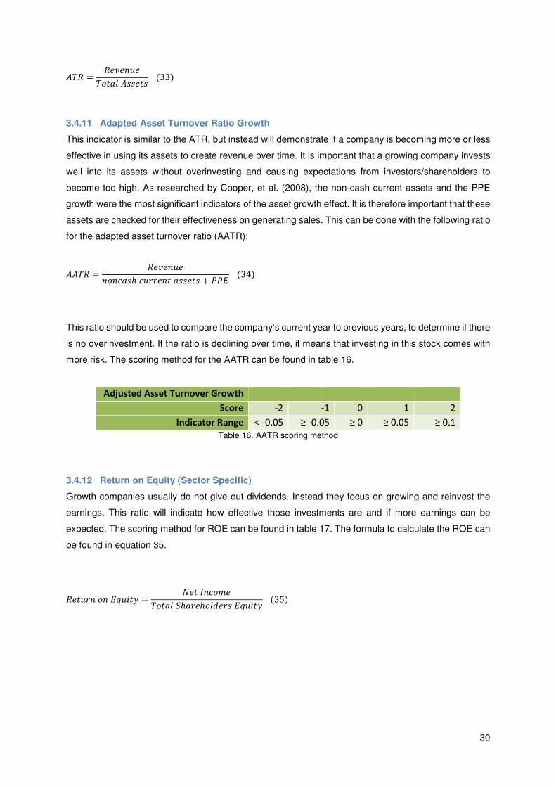
30
'"� = �)D)21)"#$%& '(()$( (33)
3.4.11 Adapted Asset Turnover Ratio Growth
This indicator is similar to the ATR, but instead will demonstrate if a company is becoming more or less
effective in using its assets to create revenue over time. It is important that a growing company invests
well into its assets without overinvesting and causing expectations from investors/shareholders to
become too high. As researched by Cooper, et al. (2008), the non-cash current assets and the PPE
growth were the most significant indicators of the asset growth effect. It is therefore important that these
assets are checked for their effectiveness on generating sales. This can be done with the following ratio
for the adapted asset turnover ratio (AATR):
''"� = �)D)21)2#2=%(ℎ =1++)2$ %(()$( + 334 (34)
This ratio should be used to compare the company’s current year to previous years, to determine if there
is no overinvestment. If the ratio is declining over time, it means that investing in this stock comes with
more risk. The scoring method for the AATR can be found in table 16.
Adjusted Asset Turnover Growth
Score -2 -1 0 1 2
Indicator Range < -0.05 ≥ -0.05 ≥ 0 ≥ 0.05 ≥ 0.1
Table 16. AATR scoring method
3.4.12 Return on Equity (Sector Specific)
Growth companies usually do not give out dividends. Instead they focus on growing and reinvest the
earnings. This ratio will indicate how effective those investments are and if more earnings can be
expected. The scoring method for ROE can be found in table 17. The formula to calculate the ROE can
be found in equation 35.
�)$1+2 #2 4G1;$H = A)$ �2=#C)"#$%& �ℎ%+)ℎ#&F)+( 4G1;$H (35)

31
Return on Equity Score
-2 -1 0 1 2
Health Care < 0.05 ≥ 0.05 ≥ 0.1 ≥ 0.15 ≥ 0.2
Consumer Discretionary < 0 ≥ 0 ≥ 0.02 ≥ 0.07 ≥ 0.15
Information Technology < 0.05 ≥ 0.05 ≥ 0.1 ≥ 0.15 ≥ 0.2
Consumer Staples < 0.05 ≥ 0.05 ≥ 0.1 ≥ 0.15 ≥ 0.3
Industrials < 0.05 ≥ 0.05 ≥ 0.1 ≥ 0.15 ≥ 0.2
Energy < 0.04 ≥ 0.04 ≥ 0.07 ≥ 0.1 ≥ 0.15
Materials < 0.04 ≥ 0.04 ≥ 0.08 ≥ 0.12 ≥ 0.16
Utilities < 0.03 ≥ 0.03 ≥ 0.06 ≥ 0.09 ≥ 0.12
Financials < 0.05 ≥ 0.05 ≥ 0.08 ≥ 0.11 ≥ 0.14
Telecommunications
Services
< 0.04 ≥ 0.04 ≥ 0.08 ≥ 0.12 ≥ 0.16
Table 17. Scoring for ROE indicator
3.5 Evolutionary Algorithm
A genetic algorithm will be used to optimize the use of the fundamental indicators. The optimizing is
done with the scoring methods of indicators presented earlier. Based on this the best stocks will be
selected to enter the portfolio. The system must however keep updating the financial data, especially
during periods of the release of financial statements. After updates, a stock in the portfolio may run out
of favor based on the newly obtained information (earnings may have declined for example). It is not
necessary to optimize when to use which technical indicator with the EA. Optimizing the technical
indicators would be more desirable when it is required to maximize return from the smaller fluctuations
in stock price.
The algorithm will require a training period after it has been programmed. This training is done using
historic data. It would be most ideal if the market circumstances are similar to those of the time period
the trading system will be used in.
Programming was done using the software Microsoft Visual Studio 2010, in the programming language
C++.
3.6 Conclusion
This chapter described the general approach for the thesis work. The trading system will be looking for
stable growth stocks that are relatively cheap. The goal is to manage a portfolio of stocks that will
outperform the S&P500 index in terms of ROI. Explanations were given on why and when to use which
technical and fundamental indicators. Indicators which were not yet presented with a formula in chapter
2, were presented with one now. All fundamental indicators also received a scoring method. This scoring
method will be used for the optimization process which will be explained in the next chapter. The financial
data resources were given and it was explained in short how a EA can be integrated to help optimize
this trading system.

32
4 Genetic Evolutionary Algorithm
This chapter starts by describing what a chromosome is and what information it holds. Then it will
describe in detail how chromosomes will undergo an evolutionary process through combination with
other chromosomes and mutations. It also discusses how the best chromosomes are selected by their
fitness. After undergoing the evolutionary process, chromosomes will be simulated. How this simulation
takes place will be described and which additional parameters are used in the trading simulator. The
way the stocks are selected to enter the portfolio is described for the short and long term systems. At
the end of the chapter it is explained how the simulation results are evaluated.
4.1 Chromosome Structure
A solution can be represented on a chromosome. The chromosome contains all the parameters to get
to the solution. These parameters are stored on the genes of that chromosome. In this trading system
there are eleven indicators, which will form the first part of the chromosome. The rest of the chromosome
will contain the other trading system’s parameters, such as: PER-filter, MA-filter, Stop-loss and cash
distribution. The standard approach to a chromosome is presented in figure 10 below.
Figure 10. Standard Chromosome Structure
The trading system used for this research, however, focusses on using only four of the eleven weighted
indicators. The thought behind this concept is, that it is more practical as a trader to only focus on a few
indicators. Since there are only four indicators, the minimum weight of a gene will be 1, with a total
weight of 100 for all four genes used. An example of what a random chromosome of the trading system
would look like, can be found in figure 11.
Figure 11. Chromosome with four indicators
4.2 Evolutionary Process
As stated before, the chromosomes represent possible solutions (positive and negative) to a portfolio of
stocks to use for trading on the S&P500 index. To try and optimize the profit of the portfolio, the EA must

33
find the best combinations of genes (weighted indicators). This is done during a training period, where
the chromosomes are evaluated by the their profit. The first step would be to create random
chromosomes.
4.2.1 Individual Fitness
The fitness of an individual chromosome is measured by the profit of the portfolio this individual leads
to. Each indicator (I) has a score for each stock ranging between -2 and 2, with 2 being the best score
possible. The indicator’s score is then multiplied with its Weight (W). The full calculation for a stock’s
score can be found in equation 36 below. The fitness of an individual is the average profit of the 20
stocks with the highest scores.
�=#+) �$#=>Y = �� ∗ t� + �q ∗ tq + �� ∗ t� + �u ∗ tu (36)
4.2.2 Population
The population contains a certain number of chromosomes. These individual chromosomes will later be
paired up with each other to form new chromosomes (children), which are a combination of the two
(parent-)chromosomes.
To start, an initial population had to be created. The EA starts by creating four totally random
chromosomes. Some rules for this process are that each indicator-gene can only be present on a
chromosome once and the minimum weight of the indicator is 1, and a maximum of 97. From the four
randomly created chromosomes, the one with the highest profit in the training period survives and is
written to a file, whilst the other three are eliminated. This process will repeat until the population size
has been achieved. For this trading system the population size was set to 128 individuals. At first the
population size was set at 64 individuals, but during the optimization process it was observed that the
solutions were converging towards a single point too quickly, without considering other solutions. These
other solutions could be better, so by increasing the population size, the number of random solutions
and combinations is also increasing. This means that the search range for solutions was also increased
to one with more possible solutions.
4.2.3 Crossover & Reproduction
After the creation of the initial population, it must form a new and more optimal generation. This is done
by combining the indicator genes of two parent individuals from the current population with each other.
They can be combined in different way to form the new children chromosomes. In this case, the goal is
to form two children to have a population pool with a total of 256 individuals. From this pool the 128
individuals with the highest fitness will survive and form the population of the next generation.
The first step is to assign each individual of the current population list to a random position on a new list,
ranging from position 0 to 127.
From here the position of the individual determines with which other individual it will be paired up.
Number 0 pairs up with number 1, number 2 with number 3 , number 4 with number 5 and so on.

34
Then the pair will combine (or crossover) genes to form two children. To illustrate this process, an
example is shown in figure 12.
Figure 12. Crossover Parent A with Parent B
As can be seen in figure 12, the chromosomes are cut in half and then combined with that the other half
of the other parent.
After the initial combination is made, the weights of each indicator needs to be adjusted. This is because
all the genes’ corresponding weights on the child will most likely not add up to be a total of 100. To fix
this issue, the weights of the child’s genes will be added up and then the weights are scaled back to
them totalling 100.
With this way of representing the genes that can be combined, there comes an additional problem of
possibly having duplicate genes on a single chromosome when it is just simply cutting the chromosomes
in half. To avoid having a gene being present on the chromosome more than once, the algorithm is able
to cut the chromosomes in a different position or positions. When having to pick another way to cut the
chromosomes and
recombine them, it will favour using two genes of each parent first. If this is not possible it will proceed
to using three of one parent and just one from the other. If the parent chromosomes have identical
genes, it will mix up the weight distribution to still create children with possibly a different fitness than
the parents. The order of preference for combining chromosomes is shown below in table 18, with the
most favourable combinations shown on top.

35
4.2.4 Mutation
After the best 128 individuals are selected, about 5% of them will be given a mutation. This is done to
attempt to generate more genetic diversity among the population. A mutation here means changing one
of the indicator genes to another random value, which is not yet present on that particular chromosome.
The gene to be changed is selected at random. An example of a mutation is shown in figure 13.
The concept of elitism is used to preserve the best solutions. The best 5% of the population will be
excluded from selection for mutation. The algorithm will pick the individuals for mutation at random from
the remaining available individuals (position 7 to 127 on the list).
Figure 13. Mutation of an individual
Position 1 Position 2 Position 3 Position 4
A A B B
B B A A
A B B A
B A A B
A B A B
B A B A
A A A B
B B B A
A B B B
B A A A
A A B A
B B A B
A B A A
B A B B
Table 18. Order of preference for combining parent chromosomes
36
From this algorithm, it was observed that in practice the mutated individuals often did not survive more
than one generation. Especially in later generations their fitness value was not high enough to survive
the next selection. It does however achieve its goal of creating more diversity and increase the search
range of solutions.
4.3 Trading Simulator Parameters
To see how the result of the genetic algorithm performs, a trading simulator program was created. The
simulator holds all the information regarding the settings of trading parameters (excluding indicator
genes). Properly setting the parameters is important for obtaining the desired results in terms of return.
The different trading parameters that have not been discussed yet in chapter 3, will be discussed in this
section.
4.3.1 Portfolio Size
The portfolio is set so that it can hold a maximum of 20 different stocks. There is no set minimum,
because the minimum depends more on other settings of the simulator, such as the minimum score
needed to enter the portfolio. The aim is however to have at least five different stocks in the portfolio
from the start. Depending on the strategy, the portfolio will build from there. For the long term strategy,
having a portfolio of around ten stocks is desirable to have decent diversification.
4.3.2 Minimum Score
The minimum score parameter is a filter that will evaluate if stocks have enough fundamental strength
to enter the portfolio. The scores are solely based on the fundamental indicators discussed in chapter
3. If the score is not high enough, the filter will reject the stock and proceed with evaluating the next
stock. Stocks already in the portfolio are still evaluated by score each new trading period. This is to
prevent holding stocks in portfolio of which recently added fundamental information was negative, and
it is expected the stock price will fall.
4.3.3 Stock Performance
After each trading period (one quarter year) the portfolio’s stocks are going through evaluation of their
performance during this period. The aim is to short the worst performing stocks (approximately 25%)
from the portfolio. This is done to create place for new stocks to enter, which could be more promising
for the coming period according to the most recent fundamental data.

37
4.3.4 Cash Distribution
Properly distributing the available cash to invest over the stock can be quite challenging. Giving the
stock with the highest score the majority of the investment seems logical, but does increase the risk of
losing the investment if anything goes wrong with that stock. Also this leaves only a small amount left to
distribute among the other stocks that also made it into the portfolio. Since the exact number of stocks
to enter the portfolio is not predetermined, the simulator will distribute the available cash over the stocks
depending on the number of new stocks to enter the portfolio. The values of distribution can be found in
table 19.
Stock Position on List
Number of
new stocks
1-2 3-4 5-7 8-11 12-15 16-20 Total (%)
20 15 10 8 3 2 1 99
19 15 11 8 3 2 1 100
18 15 11 8 3 2 1 99
17 15 12 8 3 2 1 100
16 15 12 8 3 2 1 99
15 16 12 8 3 2 0 100
14 16 13 8 3 2 0 100
13 17 13 8 3 2 0 100
12 17 14 8 3 2 0 100
11 18 14 8 3 0 0 100
10 18 14 9 3 0 0 100
9 19 14 9 3 0 0 99
8 21 14 9 3 0 0 100
7 22 14 9 0 0 0 99
6 26 15 9 0 0 0 100
5 30 15 10 0 0 0 100
4 30 20 0 0 0 0 100
3 35 30 0 0 0 0 100
2 50 0 0 0 0 0 100
1 100 0 0 0 0 0 100
Table 19. Cash Distribution over Stocks (in %)

38
4.4 Trading Strategy Systems
As discussed in chapter 3, two investment systems with different strategies will be tested. The strategy
for each system will be discussed below including a flowchart for the stock selection of each system.
4.4.1 Long Term System
The long term investment system is designed to buy potentially stable growth stocks and to hold on to
them for as long the growth is continuing. It will build up a portfolio in the first four quarters, by investing
25% of the total available cash each quarter. Since the portfolio does not have to be complete instantly,
it will only pick the best stocks. Therefore only the fifteen stocks with the highest scores are evaluated
with the earlier described filters. For a clear overview of stock evaluation for the long term, see the flow
chart in figure 14. Investment simulation will start on 15-02-2013, with the preceding year used as the
training period to optimize the use of the fundamental indicators.
4.4.2 Short Term System
The short term investment system is only looking to buy stocks that will grow in the upcoming quarter.
After each quarter it will sell the entire portfolio and select new stocks to invest in, using the total available
capital. This method does not allow to increase the portfolio size over time. Therefore the number of
highest scoring stocks that are evaluated with the parameters for portfolio entry is increased to 40 (twice
the portfolio size). Also the minimum score parameter is removed. These alterations were necessary to
increase the portfolio’s diversification in some quarters.
It will start simulation on 15-05-2012, with the preceding quarter acting as the first training period. Each
next quarter, it will update the training results with optimizations of the last period. This needs to be done
for the short term system, because it is quite likely one quarter cannot represent the upcoming trading
quarters properly in terms of growth characteristics. The aggregated training data will form the new
indicators used. It will only use the four indicators with the total highest weights from the training periods.
A flow chart of this system can be found in figure 15.

39
Figure 14. Flowchart long term stock selection

40
Figure 15. Flowchart short term stock selection

41
4.5 Portfolio Performance Evaluation Methods
To evaluate the fitness of an individual in optimization or the performance of a portfolio in simulation,
the methods of ROI, Information Ratio and Pareto Dominance can be used. This section will describe
how ratios are calculated and how they should be interpreted.
4.5.1 Return On Investment
The ROI (or profit) is the most simple way to evaluate both the portfolio performance and the fitness of
individuals. It is used in single-objective optimization as the only evaluation method of individuals. The
ROI for optimization can be calculated using equation 37. Equation 38 can be used for calculating the
ROI for portfolio performance.
�5� = 3�Y� � ∗ 3�h��h �3�h��h � + 3�Y� v ∗ 3�h��h v3�h��h v + ⋯ + 3�Y� v ∗ 3�h��h v3�h��h v20 (37)
Where: Pstart i = Price of stock i at the beginning of training period
Pend i = Price of stock i at the end of training period
�5� = 42F /%9;$%& − �2;$;%& /%9;$%&�2;$;%& /%9;$%& (38)
Where: Capital = Cash + Outstanding Equity
4.5.2 Variance & Standard Deviation
The variance and standard deviation of the portfolio’s return will be used as a measurement of risk for
the multi-objective approach to optimization. The variance is used for the Pareto-Dominance concept,
while standard deviation is used for the Information Ratio. The variance and standard deviation can be
calculated through equation 39. Because the trading system is only reviewing entire the portfolio each
quarter (with exception of the daily stop-loss check), the standard deviation and variance are annualized
from quarterly data when needed.
Xv = ∑(wV − x)v2 (39)
Where: σ2 = variance
σ = standard deviation
Xi = ROI of stock i
μ = average ROI of portfolio
n = number of stocks in portfolio

42
4.5.3 Sharpe Ratio & Information Ratio
The Sharpe ratio is the industry standard for measuring the risk-adjusted return. It was originally
developed as a ratio to determine the expected reward from investing in a risky asset versus a risk-free
asset. Like expected returns it can also be used to calculate the actual risk-adjusted return (Kidd, 2011).
The Sharpe ratio can be calculated using equation 40.
�� = �y − ��Xy (40)
Where: σp = standard deviation of portfolio
Rp = average return of portfolio
Rf = return of risk-free asset
An example of a risk-free asset is a U.S. treasury bill. The interest rates of the U.S. treasury bills can be
found in figure 16. As can be seen there, the interest rate is really low over the maturity periods of three
months and one year. When investing into a bill with longer maturity, the interest/return is higher, but it
is better to compare to the previously mentioned timespans because they correspond more to the
timespan of the trading simulations.
With these low return-rates on the risk-free asset, it seems kind of pointless to compare the simulation
return results to a risk-free asset. Also this thesis is about growth stocks, meaning it is supposed to trade
in stocks with a higher than average growth. Therefore the Sharpe ratio will not be used to evaluate
trading performance. Instead the evaluation will done through the Information ratio, a variant of the
Sharpe ratio.

43
Figure 16. Historical Return rates for U.S. treasury bills (source: treasury.gov)
The information ratio compares the portfolio return versus a benchmark return. This benchmark is what
replaces the risk-free asset in the Sharpe ratio. The standard deviation of portfolio in the Sharpe ratio’s
formula is replaced by the standard deviation of the difference between the portfolio’s return and that of
the benchmark, also called the tracking error. The Information ratio will tell how much excess return is
generated from the excess risk taken (Kidd, 2011). In this case the benchmark will be the S&P500 index.
The Information ratio can be calculated with equation 41. The tracking error can be calculated with the
formula in equation 42.
�� = �y − �zXyiz (41)
Where: σp-b = tracking error
Rp = average return of portfolio
Rb = return of benchmark
σyiz = |∑(�yh − �zh)v2 − 1 (42)
Where: n = number of trading periods
Rpt = average return of portfolio, in trading period t
Rbt = return of benchmark, in trading period t

44
4.5.4 Pareto Dominance
The Pareto Dominance concept will be applied for multi-objective optimization. It will help to find
solutions where the ROI is maximal and the variance is minimal. The non-dominated solutions will form
the Pareto frontier. Depending on the risk profile the investor wants to take, a solution can be picked.
The non-dominated solutions that appear the most interesting based on their variance relative to their
expected ROI will be picked and simulated. The results can be found in the next chapter.
4.6 Conclusion
This chapter started by explaining that a chromosome is formed by genes of fundamental indicators and
their respective weights. The EA will combine random chromosomes of a population of 128 individuals
with each other to form two new chromosomes for each pair. The best 128 individuals from that total
population will form the next generation. Chromosomes are limited to having four indicator genes.
In simulation, the portfolio can hold a maximum of 20 different stocks. There are two simulation
strategies, one is short term and the other is long term. The short term system will form a totally new
portfolio each quarter and has multiple training periods of one quarter. The long term system is looking
to build a portfolio over time and depending on their evaluation, it will hold stocks in the portfolio after
each quarter and add new ones to the existing portfolio. The long term system has a single training
period of one year. Evaluating the trading of the systems will be done using the ROI and the Information
ratio. The benchmark used for calculating the Information ratio is the S&P500 index. For the multi
objective approach, the Pareto dominance concept is used to select which chromosomes will be
simulated.

45
5 Results
This chapter describes and discusses the results obtained in simulation using the optimized
chromosomes found with the EA. The first results that are discussed will be that of the short term single
objective system. Then the results of the long term single objective system are discussed and finally it
will show the results of the multi objective system that used the Pareto dominance concept.
To keep the results more organized, the fundamental indicators are numbered as they are on the
chromosomes used in the EA. For reference, the gene number for each indicator can be found in table
20.
Gene Number Fundamental Indicator
1 Revenue Growth
2 Earnings per Share Growth
3 Profit Margin Growth
4 Adjusted Asset Turnover Growth
5 Debt Growth
6 Revenue vs. Debt Growth
7 Company Sector
8 Profit Margin (Sector Specific)
9 Return on Equity (Sector Specific)
10
Asset Turnover Ratio (Sector
Specific)
11 Debt Ratio (Sector Specific) Table 20. Indicator number reference table
5.1 Single Objective Short Term
The first simulations were done for the short term system, optimizing for the single objective ROI.
Training periods had a length of one quarter and each new trading period, the training results of the
preceding quarter were added to the training results. From this the new indicators were chosen based
on which four indicators were the most present in terms of weight.
In total three simulations were done, creating the dynamic chromosomes S1 to S3. S1 had a selection
of chromosomes from the best chromosome from each training period. S2 is similar to S1, but the
training periods were ran once more and the best chromosomes were selected, except ones that were
similar to chromosomes in S1. For S3 the same training results were used as for S2, but S3 did get
chromosomes that were slightly lower in terms of ROI and at least one gene different from S2.
The training results can be found in table 21 for S1, table 22 for S2 and table 23 for S3. Training period
0 (T0) started at 15-02-2012 and ended 15-05-2012. T1 are the training results for the next quarter and
so on. At the end of each table the final dynamic chromosome composition is shown with the weights,
as used in trading quarter 11.

46
Training
Period
1st
Gene
2nd
Gene
3rd
Gene
4th
Gene
Weight
1st
Gene
Weight
2nd
Gene
Weight
3rd
Gene
Weight
4th
Gene
T0 9 6 2 8 59 10 24 7
T1 4 10 1 7 65 7 6 22
T2 7 4 3 2 59 21 11 9
T3 1 6 11 4 56 31 6 7
T4 4 7 10 1 36 33 5 26
T5 5 2 8 1 73 19 3 5
T6 7 5 2 4 60 26 7 7
T7 1 4 8 11 40 27 10 23
T8 7 1 6 2 72 5 2 21
T9 9 4 1 7 35 11 43 11
T10 7 10 1 11 37 34 26 3
Final 1 4 5 7 207 174 99 294
Table 21. Training results chromosome S1
Training
Period
1st
Gene
2nd
Gene
3rd
Gene
4th
Gene
Weight
1st
Gene
Weight
2nd
Gene
Weight
3rd
Gene
Weight
4th
Gene
T0 9 6 7 2 65 9 4 22
T1 6 4 11 7 19 65 13 3
T2 7 4 5 2 61 20 8 11
T3 6 5 2 4 66 18 12 4
T4 4 7 6 10 34 31 23 12
T5 8 4 11 9 26 34 26 14
T6 7 5 6 4 63 17 15 5
T7 11 1 7 3 28 40 15 17
T8 7 1 5 2 82 5 4 9
T9 4 3 1 2 7 11 76 6
T10 10 3 1 11 70 7 17 6
Final 1 4 6 7 138 169 132 259
Table 22. Training results chromosome S2

47
Training
Period
1st
Gene
2nd
Gene
3rd
Gene
4th
Gene
Weight
1st
Gene
Weight
2nd
Gene
Weight
3rd
Gene
Weight
4th
Gene
T0 9 6 3 2 64 10 8 18
T1 4 1 6 10 31 32 22 15
T2 9 7 5 4 62 28 7 3
T3 5 6 2 4 32 51 6 11
T4 4 7 6 2 39 39 19 3
T5 9 11 1 8 51 24 13 12
T6 7 5 6 4 52 28 15 5
T7 11 1 7 3 19 38 22 21
T8 7 2 1 10 67 22 5 6
T9 1 11 2 7 63 15 10 12
T10 10 3 1 11 57 7 26 10
Final 1 6 7 9 177 117 220 177
Table 23. Training results chromosome S3
Simulation of these chromosomes started on 15-05-2012 and ended on 15-02-2015. The results are
presented in growth rates for each quarter in table 24. The total growth, tracking error and Information
ratio can be found in table 25.
Q1
ended
15-8-
2012
Q2
ended
15-11-
2012
Q3
ended
15-2-
2013
Q4
ended
15-5-
2013
Q5
ended
15-8-
2013
Q6
ended
15-11-
2013
Q7
ended
15-2-
2014
Q8
ended
15-5-
2014
Q9
ended
15-8-
2014
Q10
ended
15-11-
2014
Q11
ended
15-2-
2015
S1 0.033 -0.023 0.137 0.131 0.004 0.117 0.042 0.021 0.044 0.027 0.067
S2 0.032 -0.019 0.137 0.091 -0.019 0.104 0.030 0.056 0.049 0.008 0.048
S3 0.034 -0.015 0.055 0.121 -0.017 0.127 0.009 0.052 0.042 0.050 0.074
S&P500 0.056 -0.037 0.123 0.091 0.002 0.082 0.022 0.018 0.045 0.043 0.028
Table 24. Simulation growth rate results single objective, short term
Chromosome
Combination
Total
ROI
Tracking
Error
IR
S1 0.772 0.024 8.078
S2 0.637 0.023 2.710
S3 0.664 0.035 2.510
S&P500 0.576 0.000 X
Table 25. Simulation results single obj. short term
The results show that generally speaking each chromosome outperformed the index. In the first quarter
each chromosome performed worse than the index, but this was expected because the chromosomes
only had training data of a single quarter and that quarter was not likely to be similar to the next. The
following quarter (Q2), all chromosomes already showed a better growth rate than the index.
Chromosome S1 has performed the best of all chromosomes with a ROI of almost 0.2 higher. It also

48
shows a low tracking error. Tracking error does not tell the whole story properly though, because it does
not take into account if the difference was positive or negative compared to the benchmark index. A
closer look at the data in the table reveals that S1 mostly had a positive difference compared to the
index except the final quarter.
Overall the short term strategy with rebuilding an entire portfolio each quarter does not perform greatly.
For a period of eleven quarters, the total ROI of each chromosome compared to the index seems a bit
on the low side, especially that of S2 and S3. The stock selection method also showed it has quite some
risk to it, because simulation has shown a stop-loss intervention at various quarters for stocks in the
portfolio. This could possibly be caused by the lack of a minimum score parameter, but this parameter
was left out to increase the overall portfolio size and add diversification.
5.2 Single Objective Long Term
The next simulations were done using single objective optimization for ROI. This time the simulation
system is looking for stocks on the long term. The training period of one year was done from 15-05-2012
till 15-05-2013. Then five chromosomes were picked from the population which went through 20
iterations in the genetic EA. The chromosome selection is based on the maximum value of ROI, but the
chromosomes must have at least one gene different from another.
It must be noted however that the chromosome with the highest ROI was not selected here, because
this is a non-dominated solution for the multi-objective approach. The simulation results of that
chromosome can be found in the next section as chromosome M13.
The composition of the five selected chromosomes can be found in table 26.
Chromo-
some # ROI
1st
Gene
2nd
Gene
3rd
Gene
4th
Gene
Weight
1st
Gene
Weight
2nd
Gene
Weight
3rd
Gene
Weight
4th
Gene
L1 0.549117 5 1 4 2 27 54 8 11
L2 0.538764 1 5 2 6 56 18 10 16
L3 0.526488 6 1 3 2 30 38 18 14
L4 0.519741 1 5 2 6 29 29 15 27
L5 0.508123 1 5 10 11 41 33 22 4 Table 26. Chromosome composition, single objective long term
The simulation period started on 15-5-2013 and ended on 15-2-2015. The simulation results are
presented in growth rates in table 27. It also shows the tracking error and Information ratio for each
chromosome.

49
Chromo-
some # Q1 Q2 Q3 Q4 Q5 Q6 Q7
Compounded
Growth
Tracking
Error IR
L1 -0.003 0.086 -0.155 0.034 0.047 -0.015 0 -0.025 0.077 -3.727
L2 0.011 0.099 -0.051 -0.013 0.014 0.025 0.041 0.126 0.037 -3.723
L3 0.016 0.074 -0.04 0.007 0.076 -0.007 0.008 0.138 0.037 -3.441
L4 -0.029 0.081 -0.036 -0.012 0.005 -0.072 0.071 -0.002 0.06 -4.407
L5 -0.027 0.086 -0.011 0.04 0.053 0.093 0.05 0.313 0.03 1.628
SP500
Index 0.002 0.082 0.022 0.018 0.045 0.043 0.028 0.264 0 X Table 27. Simulation quarterly growth rates, single objective long term
The results show that four out of five chromosomes were beaten by the index in terms of compounded
growth. This is displayed as a negative Information Ratio. Also the interpretation of the IR is hard for
negative values, because normally a higher value is better, but here it can be seen that the worst profit
with the highest risk (highest tracking error) has an IR similar to one with a superior profit and lower risk
(tracking error).
Each chromosome has revenue growth as its main indicator, but only L5 has a positive ROI compared
to the benchmark index. Possibly this indicator comes with added risk. Before drawing any conclusions,
the multi-objective simulation results will be checked. This may give a better insight in the characteristics
of certain indicators.
5.3 Multi Objective Long Term
For the Multi Objective Long Term approach, the training period was done from 15-05-2012 to 15-05-
2013. Generating the Pareto front was done by extracting the population from different generations of
the EA. The population was taken from the initial population (generation zero), the first generation, the
fifth generation, the tenth generation and finally the twentieth generation. All individuals/chromosomes
were then plotted into a graph. The result can be seen in figure 17.

50
Figure 17. Training results plotted
The red dots in the graph represent the non-dominated individuals and the green dots are the dominated
individuals. The non-dominated individuals that appear to be the most interesting because of their ROI
relative to their variance, are connected by a grey line. These are the individuals that will be simulated
over the period of 15-05-2013 till 15-02-2015. More details about the composition of these individuals
can be found in table 28.
Variance ROI
1st
Gene
2nd
Gene
3rd
Gene
4th
Gene
Weight
1st
Gene
Weight
2nd
Gene
Weight
3rd
Gene
Weight
4th
Gene
M1 0.027623 0.247262 3 1 8 10 83 1 3 13
M2 0.044887 0.299454 3 7 2 6 77 18 2 3
M5 0.064502 0.365611 2 1 3 6 12 24 53 11
M6 0.140695 0.394648 7 5 1 6 55 8 6 31
M9 0.232294 0.464276 5 1 2 3 13 32 17 38
M11 0.371682 0.532761 1 6 2 3 68 15 9 8
M13 0.456967 0.567565 5 1 2 4 44 32 19 5
Table 28. Non-dominated Solutions from Training period
The training results show that this selection of chromosomes all have a gene for either revenue growth
or earnings growth, although chromosome M1 only has a weight of 1 invested into revenue growth,
which is the minimal weight possible to invest in a gene. The gene for profit margin growth also often
appears in the chromosomes.
The results of simulating all these chromosomes can be found in table 29. The results are presented in
growth rates, to make them easy to compare to other results. The tracking error and Information ratio

51
(IR) can be found in the last columns of the table. The growth rates of the S&P500 index are shown at
the bottom, which was the benchmark to compare the chromosomes performances with.
Chromo-
some #
Q1 Q2
Q3 Q4 Q5 Q6 Q7 Compounded
Growth
Tracking
Error
IR
M1 -0.018 0.079 0.049 0.029 0.033 0.064 0.072 0.348 0.025 3.374
M2 -0.005 0.077 0.032 0.029 0.071 0.049 0.050 0.340 0.016 4.888
M5 0.004 0.082 0.020 0.050 0.104 0.032 0.042 0.382 0.028 4.151
M6 0.021 0.080 0.014 0.042 0.036 0.029 0.040 0.291 0.016 1.675
M9 0.022 0.076 0.040 0.048 0.064 0.050 0.045 0.398 0.020 6.746
M11 0.008 0.085 -0.086 0.008 0.073 -0.021 -0.014 0.045 0.056 -3.950
M13 0.032 0.092 -0.020 0.051 0.033 0.060 0.029 0.309 0.027 1.637
S&P500 0.002 0.082 0.022 0.018 0.045 0.043 0.028 0.264 0.000 X
Table 29. Multi Objective simulation results, presented in growth rate
The results show that almost every chromosome has a positive Information ratio and thus outperformed
the S&P500 index. Only one chromosome performed poorly, which was chromosome M11. This
chromosome also has a high tracking error, double that of the next highest tracking error. This means
the performance was volatile compared to the index. To get a better view of the chromosomes’ growth
rate stability, they were plotted into a graph, which can be found in figure 18.
Figure 18. Growth rates of Multi Objective Chromosomes in each trading quarter
In the graph of figure 18, it becomes clear that M11 has a major drop in Q3. It then slowly recovers and
has more growth in Q5 than the index. After this it drops again below the index growth though.
Another thing that instantly stands out is the performance of chromosome M5 in Q5, where it gets over
10% growth.

52
M9 has a better performance than the index in each quarter, with the exception of Q2. This shows that
tracking error (like variance and standard deviation) can be misleading as a risk measuring tool, since
M9 has a higher tracking error than e.g. M6, but M9 only went slightly under the index in a single quarter.
Overall the results show that the chromosomes selected with the multi-objective approach perform very
well, with above index average results.
5.4 Chromosome Composition Analysis
In section 5.2 it was observed that the chromosomes with the highest ROI in the training period all had
the gene for revenue growth in them with a substantial weight. The simulation that followed showed that
only one out of these five genes produced a total compounded growth rate that was higher than that of
the S&P500 index average.
Section 5.3 showed better results and the only chromosome that performed worse than the index, was
also the only chromosome that had revenue growth as its most weighted gene. From these results it
can be concluded that using revenue growth as a main indicator to find the best stocks does have its
limitations, regarding the type of growth stock that is looked for. During training there is no PER-filter to
take out the relative expensive stocks and thus it can also put the expensive and rapidly growing stocks
in the virtual portfolio to calculate the average ROI. But this system was designed to find a more stable,
growth stock for the long term, with a lower risk of a great drop in price.
The non-dominated solutions that did not rely on revenue growth that much, showed a good, above
index average and stable performance. From all this it can be concluded that revenue growth is not a
good main indicator for stable growth stocks.
The indicator that appears to stand out in performance for stable growth stocks is the profit margin
growth. It is the main indicator in four non-dominated chromosomes and these four chromosomes also
had the highest total compounded growth rate. They are also the chromosomes with the highest
Information ratio of all simulations, so based on the results found in the simulations, profit margin growth
is the main indicator for stable growth stocks.
This could be explained by the fact that companies that improve their profit margin continuously, are
reducing their costs by optimizing their company processes and operations. This helps them to create
a more stable company, which in turn can be attractive to long term investors.
5.5 Stock Selection Analysis
To verify if the entire system does indeed find stable growth stocks, the portfolio of the best performing
chromosomes is checked and the important stocks that appear often in the good portfolio will be
highlighted in this section. Also the portfolio of chromosomes with a bad performance is shortly analyzed
to see why the return is lower.
The first stock that stands out is RHI. This stock is present in the portfolio of chromosome M9 (full
transaction list in Appendix A) in each quarter. It was selected as the first stock to enter the portfolio.
After Q2 it was thrown out for being one of the stocks with the worst performance, but it was bought
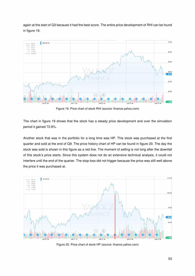
53
again at the start of Q3 because it had the best score. The entire price development of RHI can be found
in figure 19.
Figure 19. Price chart of stock RHI (source: finance.yahoo.com)
The chart in figure 19 shows that the stock has a steady price development and over the simulation
period it gained 72.8%.
Another stock that was in the portfolio for a long time was HP. This stock was purchased at the first
quarter and sold at the end of Q9. The price history chart of HP can be found in figure 20. The day the
stock was sold is shown in this figure as a red line. The moment of selling is not long after the downfall
of this stock’s price starts. Since this system does not do an extensive technical analysis, it could not
interfere until the end of the quarter. The stop-loss did not trigger because the price was still well above
the price it was purchased at.
Figure 20. Price chart of stock HP (source: finance.yahoo.com)
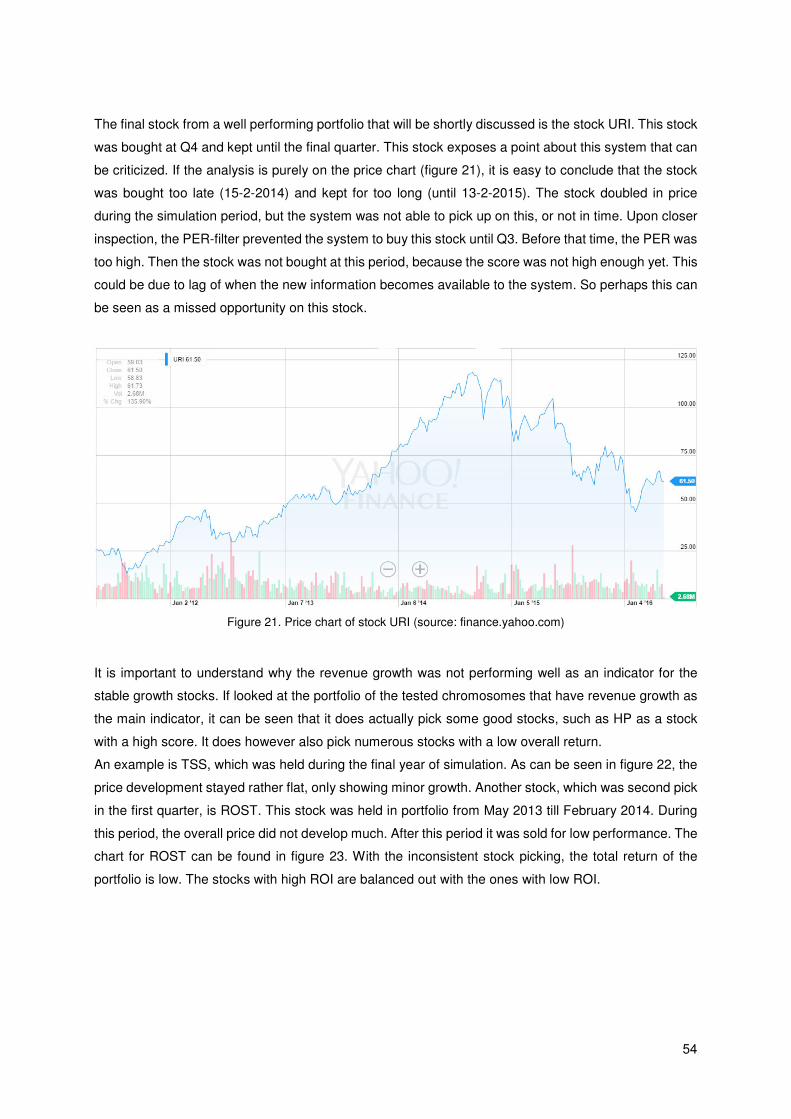
54
The final stock from a well performing portfolio that will be shortly discussed is the stock URI. This stock
was bought at Q4 and kept until the final quarter. This stock exposes a point about this system that can
be criticized. If the analysis is purely on the price chart (figure 21), it is easy to conclude that the stock
was bought too late (15-2-2014) and kept for too long (until 13-2-2015). The stock doubled in price
during the simulation period, but the system was not able to pick up on this, or not in time. Upon closer
inspection, the PER-filter prevented the system to buy this stock until Q3. Before that time, the PER was
too high. Then the stock was not bought at this period, because the score was not high enough yet. This
could be due to lag of when the new information becomes available to the system. So perhaps this can
be seen as a missed opportunity on this stock.
Figure 21. Price chart of stock URI (source: finance.yahoo.com)
It is important to understand why the revenue growth was not performing well as an indicator for the
stable growth stocks. If looked at the portfolio of the tested chromosomes that have revenue growth as
the main indicator, it can be seen that it does actually pick some good stocks, such as HP as a stock
with a high score. It does however also pick numerous stocks with a low overall return.
An example is TSS, which was held during the final year of simulation. As can be seen in figure 22, the
price development stayed rather flat, only showing minor growth. Another stock, which was second pick
in the first quarter, is ROST. This stock was held in portfolio from May 2013 till February 2014. During
this period, the overall price did not develop much. After this period it was sold for low performance. The
chart for ROST can be found in figure 23. With the inconsistent stock picking, the total return of the
portfolio is low. The stocks with high ROI are balanced out with the ones with low ROI.

55
Figure 22. Price history chart of TSS (source: finance.yahoo.com)
Figure 23. Price chart of the stock ROST (source: finance.yahoo.com)
5.6 Conclusion
In this chapter all the simulation results can be found. The single objective short term system performed
decently and outperformed the index with all three solutions. The best solution from the short term
system had a ROI of 77.2% versus a 57.6% ROI of the S&P500 index. The tracking error of this solution
was 0.024.
The long term single objective system did not perform well. Five of the best solutions from the training
period were simulated and only one of them outperformed the index with a growth rate of 31.3% against
a 26.4% growth rate of the S&P500 index during that period. These solutions all had revenue growth as
their main indicator. It should be noted that chromosome M13 is also a solution present in the single
objective system though. It improves the performance to two out of six chromosomes beating the index,
but that still is not a good result.

56
The multi-objective system performed well. Seven non-dominated solutions were simulated and six of
them outperformed the index. The best solution had a growth rate of 39.8% versus an index growth of
26.4%. Most of these solutions had profit margin growth as their main indicator. The only solution that
did not beat the index had revenue growth as its main indicator.
After the simulation results were presented, the stock selection of the chromosomes was analyzed. The
good solutions from the long term multi-objective system were able to find the type of stocks it was
designed to look for; stable growth stocks with an above average growth rate.
Then it was shown that even though the chromosomes with revenue growth as the main indicator were
able to find similar growth stocks, their stock picking was inconsistent and the portfolio also had
numerous stocks that did not have good growth rates. These stocks with a lower growth rate kept the
overall portfolio performance down.
Overall it can be concluded that profit margin growth is a good main indicator to use when looking for
stable growth stocks.
57
6 Conclusions & Future Work
This thesis presented a trading system with the goal to manage a portfolio of stocks with above average
return. The desired stocks were described as stable growth stocks that are relatively cheap. The focus
was on using fundamental indicators, which were calculated using quarterly financial data from
companies on the S&P500 index. The combination of fundamental indicators was optimized with a
genetic EA, which always used a combination of four weighted indicators. Optimization was done during
training periods of one quarter or one year, depending on the investment strategy. The two applied
investment strategies were a short term and a long term one. The short term system rebuild the entire
portfolio each quarter and the long term system could hold stocks in portfolio for a longer period of time,
eliminating the worst performing stocks and adding new stocks to portfolio each quarter. The
conclusions that can be drawn from the thesis work will be presented below as well as suggestions for
future work.
6.1 Conclusions
• The multi-objective long term approach gave the most consistent results, with six out of seven
chromosomes beating the index. The best chromosome outperformed the index with 39.8%
versus 26.4% of the index.
• Single objective long term simulation gave the worst results, with only two out of six
chromosomes beating the index.
• Single objective short term performed decently, with all three simulated chromosomes beating
the index. The best performing chromosome had a ROI of 77.2% versus 57.6% ROI of the
index. The results were less consistent than the multi-objective long term approach though.
• It is possible to find stable growth stocks using only four fundamental indicators in an optimized
combination.
• Profit margin growth works the best as a main indicator for stable growth stocks.
• Revenue growth gave inconsistent results as a main indicator when selecting stocks to enter
the portfolio.
6.2 Future Work
There is still room to improve this and similar trading systems. Also it would be useful to test if this
system is able to perform well in a less consistent market. Quarterly data is not easy to obtain and with
the limited data available it was only possible to train the EA and simulate in a bullish market. Further
suggestions that can add to improving the trading system are:
• Adding more TA. This thesis only used a minimal number of technical indicators. Some technical
indicators to find better points of entry into the market and getting out at optimal points would
increase the overall return rates of the system.

58
• Researching flow analysis to find out if such very short term trading can benefit systems similar
to this one.
• Adding market profiles to match certain training periods to the expected market condition of the
upcoming trading period. This should benefit the overall returns because the chromosomes will
be optimized for the specific market/industry conditions.
• Testing risk indicators that can differentiate between positive and negative ‘variance’. This could
clarify which portfolios are really more risky, and which have more opportunity.
59
References Anagnostopoulos, K. & Mamanis, G., 2011. The mean-variance cardinality constrained portfolio
optimization problem: An experimental evaluation of five multiobjective evolutionary algorithms.
Expert Systems with Applications, pp. 14208-14217.
Branke, J. et al., 2008. Portfolio optimization with an envelope-based multi-objective evolutionary
algorithm. European Journal of Operational Research, pp. 684-693.
Casanova, I., 2010. Tradinnova-LCS: Dynamic stock portfolio decision-making assistance model with
genetic based machine learning. pp. 1-8.
Chang, T., Meade, N., J.E., B. & Sharaiha, Y., 2000. Heuristics for cardinality constrained portfolio
optimization. Computers & Operations Research, pp. 1271-1302.
Chan, L. & Lakonishok, J., 2004. Value and Growth Investing: Review and Update. Financial Analysts
Journal, pp. 71-86.
Chiam, S., Tan, K. & Al Mamun, A., 2009. Investigating technical trading strategy via an multi-objective
evolutionary platform. Expert Systems with Applications, pp. 10408-10423.
Cooper, M. J., Gulen, H. & Schill, M. J., 2008. Asset Growth and the Cross-Section of Stock Returns.
The Journal of Finance, pp. 1609-1651.
Corne, D., Knowles, J. & Oates, M., 2000. The Pareto Envelope-Based Selection Algorithm for
Multiobjective Optimization. Lecture Notes in Computer Science, pp. 839-848.
Deb, K., Pratap, A., Agarwal, S. & Meyarivan, T., 2002. A Fast and Elitist Multiobjective Genetic
Algorithm: NSGA-II. IEEE Transactions on Evolutionary Computation, pp. 182-197.
Edwards, R., Magee, J. & Bassetti, W., 2007. Technical Analysis of Stock Trends 9th Edition. s.l.:CRC
Press.
Erickson, M., Mayer, A. & Horn, J., 2001. The Niched Pareto Genetic Algorithm 2 Applied to the
Design of Groundwater Remediation Systems. Lecture Notes in Computer Science, pp. 681-
695.
Fama, E. & French, K., 1998. Value versus Growth: The International Evidence. The Journal of
Finance, pp. 1975-1999.
Fu, T., Chung, C. & Chung, F., 2013. Adopting genetic algorithms for technical analysis and portfolio
management. Computers and Mathematics with Applications, pp. 1743-1757.
Geva, T. & Zahavi, J., 2013. Empirical evaluation of an automated intraday stock recommendation
system incorporating both market data and textual news. Decision Support Systems, pp. 212-
223.
Gorgulho, A., Neves, R. & Horta, N., 2011. Applying a GA kernel on optimizing technical analysis rules
for stock picking and portfolio optimization. Expert Systems with Applications, pp. 14072-14085.
Graham, B., 1973. The Intelligent Investor. s.l.:Perfect Bound.
Graham, B. & Dodd, D., 1934/2009. Security Analysis 6th edition. s.l.:McGraw-Hill.
Hanne, T., 2007. A multiobjective evolutionary algorithm for approximating the efficient set. European
Journal of Operational Research, pp. 1723-1734.
Helfert, E., 2001. Financial Analysis: Tools and Techniques. s.l.:McGraw-Hill.

60
Hirschleifer, D., Hou, K., Teoh, S. & Zhang, Y., 2004. Do investors overvalue firms with bloated
balance sheets?. Journal of Accounting and Economics, pp. 297-331.
Hu, Y. et al., 2014. Stock trading rule discovery with an evolutionary trend following model. Expert
Systems with Applications, pp. 212-222.
Kaucic, M., 2012. Portfolio Management Using Artificial Trading Systems Based on Technical
Analysis. Genetic Algorithms in Applications, pp. 281-294.
Kidd, D., 2011. Investment Performance Measurement. CFA.
La Porta, R., Lakonishok, J., Shleifer, A. & Vishny, R., 1997. Good new for value stocks: Further
evidence on market efficiency. The Journal of Finance, pp. 859-874.
Markowitz, H., 1952. Portfolio selection. The Journal of Finance, pp. 77-91.
Menkhoff, 2010. The use of technical analysis by fund managers: International evidence. Journal of
Banking & Finance, pp. 2573-2586.
Murphy, J., 1999. Technical Analysis of the Financial Markets. s.l.:New York Institute of Finance.
Papanastasopoulos, G., Thomakos, D. & Wang, T., 2011. Information in balance sheets for future
stock returns: Evidence from net operating assets. International Review of Financial Analysis,
pp. 269-282.
Shiller, R. J., 2006. Irrational Exuberance. s.l.:s.n.
Shynkevich, A., 2011. Performance of technical analysis in growth and small cap segments of the US
equity market. Journal of Banking & Finance, pp. 193-208.
Silva, A., Neves, R. & Horta, N., 2014. A hybrid approach to portfolio composition based on
fundamental and technical indicators. Expert Systems with Applications, pp. 2036-2048.
Tavakoli, M., McMillan, D. & McKnight, P., 2011. Insider trading and stock prices. International Review
of Economics and Finance, pp. 254-266.
Wilder Jr., J., 1978. New Concepts in Technical Trading Systems. s.l.:Hunter Publishing Company.
Yardeni, E. & Abbott, J., 2015. Earnings, Revenues, & Valuation: S&P 500/400/600. Yardeni
Research Inc..
Zitzler, E., Laumanns, M. & Bleuler, S., 2004. A tutorial on multiobjective optimization. Metaheuristics
for Multiobjective Optimization, pp. 3-37.
Zweig, M., 1986. Winning on Wall Street. s.l.:Warner Books.
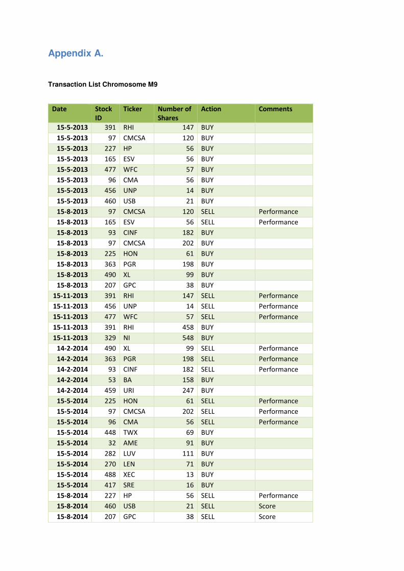
61
Appendix A.
Transaction List Chromosome M9
Date Stock
ID
Ticker Number of
Shares
Action Comments
15-5-2013 391 RHI 147 BUY
15-5-2013 97 CMCSA 120 BUY
15-5-2013 227 HP 56 BUY
15-5-2013 165 ESV 56 BUY
15-5-2013 477 WFC 57 BUY
15-5-2013 96 CMA 56 BUY
15-5-2013 456 UNP 14 BUY
15-5-2013 460 USB 21 BUY
15-8-2013 97 CMCSA 120 SELL Performance
15-8-2013 165 ESV 56 SELL Performance
15-8-2013 93 CINF 182 BUY
15-8-2013 97 CMCSA 202 BUY
15-8-2013 225 HON 61 BUY
15-8-2013 363 PGR 198 BUY
15-8-2013 490 XL 99 BUY
15-8-2013 207 GPC 38 BUY
15-11-2013 391 RHI 147 SELL Performance
15-11-2013 456 UNP 14 SELL Performance
15-11-2013 477 WFC 57 SELL Performance
15-11-2013 391 RHI 458 BUY
15-11-2013 329 NI 548 BUY
14-2-2014 490 XL 99 SELL Performance
14-2-2014 363 PGR 198 SELL Performance
14-2-2014 93 CINF 182 SELL Performance
14-2-2014 53 BA 158 BUY
14-2-2014 459 URI 247 BUY
15-5-2014 225 HON 61 SELL Performance
15-5-2014 97 CMCSA 202 SELL Performance
15-5-2014 96 CMA 56 SELL Performance
15-5-2014 448 TWX 69 BUY
15-5-2014 32 AME 91 BUY
15-5-2014 282 LUV 111 BUY
15-5-2014 270 LEN 71 BUY
15-5-2014 488 XEC 13 BUY
15-5-2014 417 SRE 16 BUY
15-8-2014 227 HP 56 SELL Performance
15-8-2014 460 USB 21 SELL Score
15-8-2014 207 GPC 38 SELL Score

62
15-8-2014 53 BA 158 SELL Performance
15-8-2014 32 AME 91 SELL Performance
15-8-2014 270 LEN 71 SELL Performance
15-8-2014 191 FTI 305 BUY
15-8-2014 323 NDAQ 435 BUY
14-11-2014 191 FTI 305 SELL Performance
14-11-2014 488 XEC 13 SELL Performance
14-11-2014 459 URI 247 SELL Performance
14-11-2014 297 MET 256 BUY
14-11-2014 449 TXN 270 BUY
14-11-2014 459 URI 60 BUY
14-11-2014 230 HRL 128 BUY
14-11-2014 59 BCR 28 BUY
6-1-2015 459 URI 60 SELL Stop Loss