† This article belongs to the Special Issue devoted to the 85th anniversary of Croatica Chemica Acta. * Author to whom correspondence should be addressed. (E-mail: bmatasov@irb.hr)

CROATICA CHEMICA ACTA CCACAA, ISSN 0011-1643, e-ISSN 1334-417X

Croat. Chem. Acta 86 (1) (2013) 57–64. http://dx.doi.org/10.5562/cca2177

Original Scientific Article

Growth Season Photochemical Pollution over the UK Based on 1990-2006 Ozone Data†

Brunislav Matasović,a,* Leo Klasinc,a and Tomislav Cvitašb

aDivision of Physical Chemistry, "Rudjer Boskovic" Institute, HR-10002 Zagreb, Bijenička c. 54, Croatia bChemistry Department, Faculty of Science, University of Zagreb, HR-10002 Zagreb, Horvatovac 102a, Croatia

RECEIVED SEPTEMBER 25, 2012; REVISED DECEMBER 11, 2012; ACCEPTED JANUARY 7, 2013

Abstract. Ozone data from 13 rural and 11 urban sites for the growth season (April through September) during 1990-2006 have been analysed on the basis of recently introduced photochemical pollution indica-tors. The indicators predict that urban sites are prone to photochemical pollution, although compared to some rural sites, the urban sites have lower average ozone concentrations and showed lower values of time for which hourly average ozone concentration is above a threshold value. Interestingly, the frequency distribution of ozone concentrations, especially the frequency of very low (close to zero) concentrations, correlates well with the average ozone volume fraction during the growth period. The present analysis shows that photochemical pollution in the UK is less severe compared with photochemical pollution in central Europe and the Mediterranean region (Italy, Croatia, Slovenia).(doi: 10.5562/cca2177)

Keywords: photochemical pollution, pollution indicators, ambient ozone, ozone monitoring, growth sea-son, average hourly ozone data

INTRODUCTION

Owing to its oxidizing capacity, elevated ozone concentra-tions in the planetary boundary layer are harmful to most life forms.1 Earth's atmosphere contains naturally occur-ring ozone transported from the stratosphere and ozone created in the troposphere by electric discharges that can break oxygen molecules into atoms that form ozone, but most ozone comes from human activities that release NO as the primary pollutant which is, than, rapidly oxidized to brown nitrogen dioxide (NO2). Photolysis by sunlight of NO2 to oxygen atoms is the main source of ozone for-mation in the troposphere. During night, in the absence of sunlight, NO2 is further oxidized to NO3· and finally to N2O5 and HNO3. Naturally occurring corresponding NOx concentrations in the atmosphere are very low (its sources being wildfires and lightning) and considerably increased values of NOx can invariably be associated with human activities (energy generation, chemical industries, transport and combustion processes). The increase in atmospheric ozone volume fractions observed worldwide nowadays is generally considered as pollution. It is pre-dicted that a further rise in tropospheric ozone concentra-tions will occur in the future2 affecting the crops.3

Ozone can be easily and reliably monitored, and based on the average hourly ozone volume fractions at

many locations over long periods of time, a number of indices, directives and air quality standards and limits have been put forward in order to quantify the air quality affecting humans, vegetation and materials.4,5 Long-term ozone monitoring results at various European locations6 have shown that along with a high daily value of ozone volume fractions, the extent of the diurnal variation expressed as the ratio of maximum to minimum ozone volume fractions gives a much better insight into the atmospheric condition known as photochemical pollu-tion (PP). The recent analysis of more than 14 years of whole-year ozone data from 18 monitoring stations in the UK by Jenkin7 revealed interesting results on trends in the ozone concentration distribution as well as on local, regional and global influences. This analysis showed that as a rule, the annual mean O3 concentration was higher in rural sites than in urban sites. It identified NOx concentrations as the main cause and state that ozone concentrations over the UK were affected by ozone transported into the UK from the Atlantic Ocean as well as by the formation of additional ozone formed photochemically from volatile organic compounds and NOx emitted over north-western Europe and transported to the UK. However, in terms of air quality, this long-term analysis does not show the expected differentiation between urban and rural locations in the UK nor provide

58 B. Matasović et al., Growth Season Photochemical Pollution

Croat. Chem. Acta 86 (2013) 57.

any ranking among the different sites as was found in central European, Mediterranean (Italy, Slovenia, Croa-tia), and even some subtropical stations.

In spite of ozone being the most abundant sub-stance in the hazardous atmospheric condition known as photosmog, there are numerous components in this reactive brew that cause adverse effects. Since ozone reaction products with VOCs – aldehydes, peroxides, radicals, peroxy acyl nitrates, quinonoids, secondary organic aerosols8 – represent very potent pollution com-ponents, new pollution indicators have been devised. In this study, we describe the PP indicators that take into account corrections for the amount of daylight ozone production and the number of hours the hourly average exceeds a chosen limiting value over a given period (here, the vegetation growth season from April 1 till September 30). We then apply these indicators on the expanded set of UK stations7 during the growth season to confirm their value in air quality assessment.

METHODS

All the data used were obtained by the UK ozone moni-toring Automatic Urban and Rural Network (AURN) set

up by the UK Department for Environment, Food and Rural Affairs (DEFRA). The locations of all the moni-toring sites are given in Table 1 and shown on the map in Fig. 1. Ambient concentrations of ozone can be ob-tained from the National Air Quality Information Ar-chive (http://uk-air.defra.gov.uk/). All the data, original-ly shown as mass concentrations in µg m–3, were con-verted to volume fractions in ppb.

The calculation method has been described previ-ously6 and was developed by analysing 10 years of ozone data from 12 European Monitoring and Evalua-tion of air Pollutants program (EMEP) stations over Europe. Originally, two indicators were proposed,

1 /P RM A (1)

and

2 exc1 168 /P R t N

where R is the average of the daily maximum-to-minimum ratios, M is the seasonal average of the daily maximum values, A is the average of all the seasonal data, texc is the number of hours in which the limit of 80

Table 1. Geographical coordinates of monitoring sites

Monitoring station Station abbrev. N Latitude Longitude Altitude

Aston Hill AH 52.504° 3.033° W 370 m

Belfast Centre(a) BE 54.616° 5.903° W 8 m

Birmingham Centre(a) BI 52.479° 1.906° W 145 m

Bottesford BO 52.929° 0.815° W 32 m

Bush Estate BU 55.859° 3.206° W 180 m

Cardiff Centre(a) CA 51.481° 3.174° W 20 m

Eskdalemuir ES 55.313° 3.204° W 269 m

Glazebury GL 53.459° 2.466° W 21 m

Harwell HW 51.573° 1.316° W 137 m

High Muffles HM 54.334° 0.807° W 267 m

Ladybower LB 53.399° 1.753° W 420 m

Leeds Centre(a) LE 53.804° 1.546° W 71 m

Liverpool Centre(a) LI 53.408° 2.981° W 20 m

London Bloomsbury(a) LO 51.521° 0.124° W 39 m

London Hillingdon(a) 51.496° 0.461° W 31 m

London Marylebone(a) 51.522° 0.155° W 36 m

London Teddington(a) 51.421° 0.340° W 13 m

Lough Navar LN 54.443° 7.872° W 130 m

Lullington Heath LH 50.793° 0.182° E 120 m

Manchester Piccadilly(a) MA 53.481° 2.238° W 45 m

Reading(a) RE 51.454° 0.955° W 44 m

Sibton SI 52.294° 0.464° E 46 m

Strath Vaich SV 57.734° 4.775° W 270 m

Yarner Wood YW 50.596° 3.715° W 119 m (a) urban station

B. Matasović et al., Growth Season Photochemical Pollution 59

Croat. Chem. Acta 86 (2013) 57.

ppb was exceeded (“excess time”) and N is the total number of hourly averages of ozone volume fractions measured.

As we can see from the above equations, both of these indicators are based on the daily maximum-to-minimum ratio R of the hourly volume fractions. The minimum value is set to 0.8 if recorded as zero. This correction of the minimum value is necessary to avoid division by zero. This reduces the possible excessive effect that slightly erroneous data close to the detection limit of modern ozone monitors would have on R. The first indicator, P1, includes, as a correction factor to R, the average of the daily maximum values M relative to the overall average A in the period of interest. This quotient, M/A, normally has a value close to 2. The second indicator, P2, includes a more sophisticated correction for the total time when a chosen limiting value (we used 80 ppb) has been exceeded. This correc-tion factor was arbitrarily adjusted so as to make the

value of P2 double that of R when the limiting value was exceeded on average once per week (168 is the number of hours per week). The third indicator, P3, which is defined as the geometrical mean of the previous two indicators, therefore includes both corrections, and ac-counts for situations when P1 and P2 differ considerably.

3 1 2P P P (3)

Thus, we have chosen P3 as the principal PP indicator for our recent analyses9,10,11 including the present one.

The three indicators should have a greater value when R is high. Since R reflects the difference between the daily maximum and minimum, and indirectly the daily ozone turnover, these indicators may also be a valid measure for adverse effects on living organisms and materials.

Maximum-to-minimum ratios depend, of course, on both the high and low values measured. The low values, close to zero, are likely to have a strong effect on the average ratio and consequently on the indicator values that are based on this ratio. This is also easily seen from the frequency distribution of the measured values.

RESULTS AND DISCUSSION

The results for the growth season (April through Sep-tember) for all the stations are shown in Table 2.

From Table 2, we can see that for all stations, the contributions of indicators P1 and P2 to P3 are similar; the values of P1 and P2 do not differ much for any given station. Thus, one may conclude that the influences of the average daily maxima (M), total ozone averages (A) and excess time (texc) values are quite similar. Indeed, higher maxima values are associated with excess time values but altogether the number of hours above the threshold of 80 ppb is quite low. For indicator P3, Table 2 shows a significant improvement at nearly all the stations after the year 2000.

Four of the eleven urban stations are in London: Marylebone and Bloomsbury, located slightly west of city centre, are 2 km apart and the other two, Hillingdon, 20 km to the west and Teddington, 20 km to the SWW are 12 km apart. The Bloomsbury station has been re-cording data since 1993, Hillingdon and Teddington since 1997 and the Marylebone records are from 1999 onwards (1998 is incomplete). A graph of P3 values over the years for these stations shows a strong correlation between the two pairs and indicates that in the years 1999 and 2003 all the stations recorded higher levels of PP.

All three Scottish stations have low indicator val-ues. Note, however, that there is no data from urban stations in Scotland.

Figure 1. Map of the UK showing the locations of the moni-toring sites. The names of the stations and their geographicalcoordinates are given in Table 1. Green squares represent lowphotochemical pollution sites, orange those of medium pollu-tion. Solid squares represent the rural sites, blank squaresrepresent the urban sites. Station abbreviations are shown inTable 1.

60 B. Matasović et al., Growth Season Photochemical Pollution

Croat. Chem. Acta 86 (2013) 57.

B. Matasović et al., Growth Season Photochemical Pollution 61

Croat. Chem. Acta 86 (2013) 57.

Both Northern Irish stations, Belfast and Lough Navar, have similar indicator values around 10, alt-hough one is urban and the other rural.

The English and Welsh stations show lower values for the rural stations than for the urban ones. Rural sta-tions Bottesford and Glazebury, as well as possibly Harwell have elevated indicator values similar to those of the nearby urban stations.

Generally, one can observe that all three indicators show high values at urban stations during the growth season. Most rural stations show lower values of all three indicators, the notable exception being Glazebury, which shows the second highest values of all stations. The fact that Glazebury is located in the vicinity of two major English cities, Manchester and Liverpool, and is affected by their industrial emissions may explain this observation. Indeed, it has already been shown for Glazebury and Bottesford stations, that their whole-year data, similar to those of urban stations, can be explained by their location near big cities.7 During the growth season, London (Hillingdon and Teddington, ahead of Bloomsbury) has the highest indicator values of all the urban stations, followed by Manchester Piccadilly, Car-diff, Liverpool, Birmingham, Leeds, and Belfast. A significant decrease in these values after the year 2000 is observed at nearly all the stations when compared with the years prior to 2000 (Table 2). This decrease, as shown also by Jenkin, would have been even more pro-nounced if the year 2003 had not been so exceptional.12 As reported earlier,6 sites with indicator values below 10 should be classified as “clean,” with 10 – 40 as “medi-

um” and sites with values above 100 as “polluted.” Thus, all rural sites Bottesford, Glazeburry, Harwell and Lough Navar would be classified as medium PP (the last two probably only up to 2003).

All covered stations at altitudes above 200 m have very low indicator values, in agreement with the find-ings for continental stations6,13 that elevated sites show lower indicator values. Note that in the British Isles, the definition of “elevated” is different than in continental Europe where only sites above 800 m are considered as elevated.

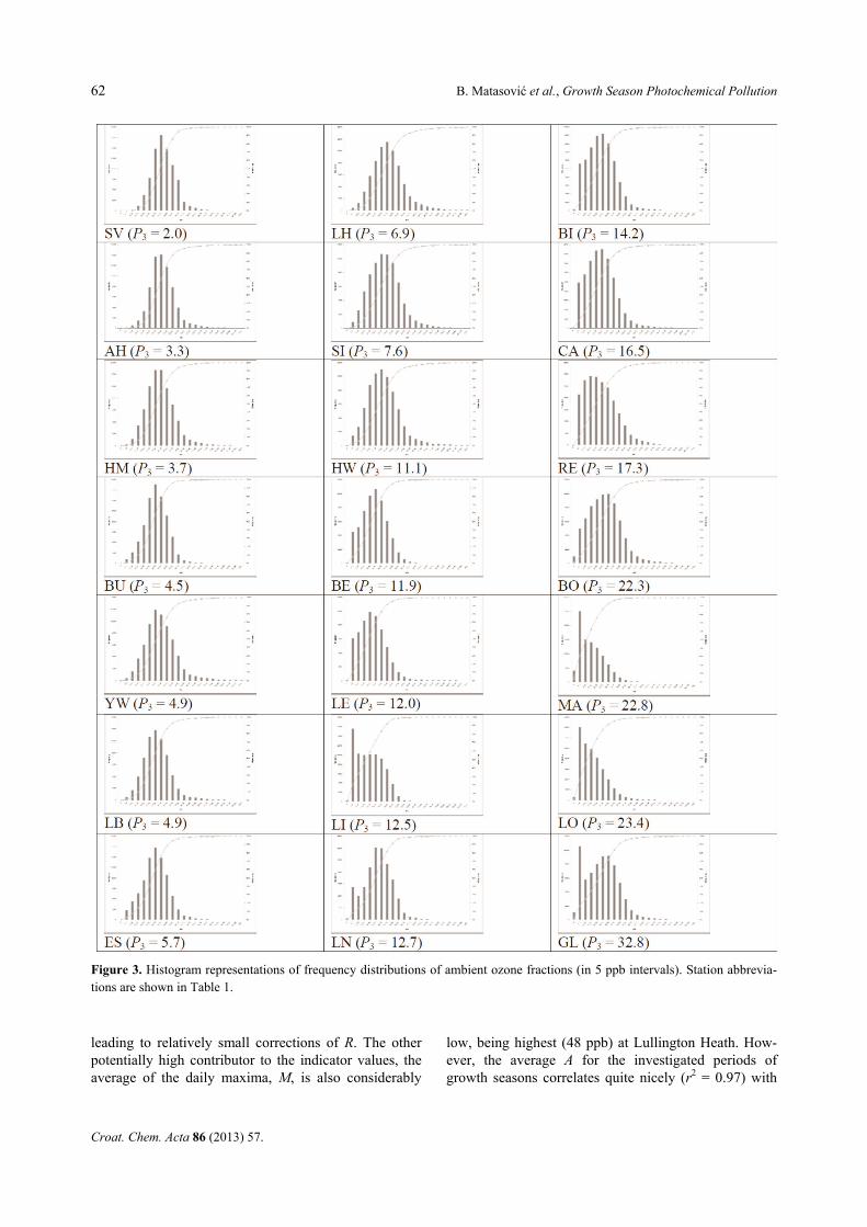
The frequency distributions of ozone volume frac-tions at the different sites can be represented by histo-grams of a box-width of 5 ppb (Fig. 3). For sites with low P3 values, the distributions show a normal (Gaussi-an) shape whereas for sites with high P3 values, the distributions differ drastically from the normal, showing a much higher frequency of low ozone volume frac-tions. The same can be said for the cumulative probabil-ity distribution, which generally follows a sigmoidal curve that spreads out as the P3 indicator increases. This is to be expected since the indicators are largely deter-mined by the average daily maximum-to-minimum ratio, R, which is necessarily higher the larger the spread of the measured values is. The indicator values become high with the number of very low hourly aver-ages as observed for Glazebury, London and Manches-ter-Piccadilly stations. None of the stations show sub-stantial excess time. In fact, only three stations (Yarner Wood, Lullington Heath and Harwell) show on average slightly more than one hour of excess time per week

Figure 2. Variations of P3 indicators at four London monitoring stations. Hillingdon (♦), Marylebone (■),Teddington (▲) and Bloomsbury (●).

62 B. Matasović et al., Growth Season Photochemical Pollution

Croat. Chem. Acta 86 (2013) 57.

leading to relatively small corrections of R. The other potentially high contributor to the indicator values, the average of the daily maxima, M, is also considerably

low, being highest (48 ppb) at Lullington Heath. How-ever, the average A for the investigated periods of growth seasons correlates quite nicely (r2 = 0.97) with

Figure 3. Histogram representations of frequency distributions of ambient ozone fractions (in 5 ppb intervals). Station abbrevia-tions are shown in Table 1.

B. Matasović et al., Growth Season Photochemical Pollution 63

Croat. Chem. Acta 86 (2013) 57.

the sum of the ozone frequency intensities for data be-tween 0 and 20 ppb.

If we compare the indicator values for stations covered in this report with those for some other regions during the early 2000s, for example, those in central Europe,6 Croatia, Italy and Slovenia,13 where P3 is gen-erally higher than 40 at urban sites (with the exception of Osijek and Rijeka where industries shrunk in the early 1990s), we conclude that the PP indicator values for the UK sites are lower than those of central and southern Europe and show a tendency of becoming even lower in future. Production of ozone in Mediterranean area is dominated by huge photochemical production of ozone in this area due to larger number of sunny days which is combined with hemispheric-scale spring max-imum.14,15 Even more, fair weather conditions favour transport of the air masses throughout the whole Medi-terranean region16 and further north in the central Eu-rope.17 Situation in the UK is somewhat different then in Mediterranean area where transport between sites highly influences the ozone levels.18 In comparison with an earlier obsrevations,6 we can, nevertheless, see the clear difference between urban and rural sites, but this transport can be the cause for lower P3 values in the urban stations in comparison with the rest of Europe since the maximum levels of hourly ozone volume frac-tions noticed in this period are not very high. This can also be seen in a Table 2 as a low texc. Still, indicator values are higher for urban sites despite the “urban decrement” of daily maxima compared with those for rural sites, which further promotes the idea of PP indica-tors which correctly point to the cities as the main pollu-tion generators.

The major advantage of the proposed PP indica-tors P1, P2 and P3 is the using of easily measured ozone concentrations to monitor overall photochemical pollu-tion caused by any pollutant monitored or omitted (for whatever reason) that may influence the ozone concen-tration. They are also in line with the fact that most air quality recommendations are based on the ozone vol-ume fractions. Their advantage is also their simplicity which is one of the major requests for the indicators to be accepted. Various other indices for ozone are in use or proposed today; AOTx – accumulated ozone expo-sure over a threshold, MPOC – maximum permissible ozone concentration,19 W95 and W126 – sum of the weighted hourly concentrations in the observed period20 and SOMO35 – sum of excess of daily maximum 8h means over the threshold of 35 ppb in a year,21 just to mention some of them. First two indices are primarily used to calculate negative impact of ozone on the health of living organisms, i.e. vegetation.

W95 and W126 are two indicators that each hourly measured concentration weights with a function that provide greater emphasis to the values above 80 ppb (W95) and 100 ppb (W126). Those two indicators,

basically, show much greater differences between pol-luted and unpolluted areas than simple hourly averaged ozone concentration.

Exposure parameter SOMO35, i.e. sum of excess of daily maximum 8-hour means over the threshold of 35 ppb in a year is based on assumption that the level of 35 ppb as daily maximum 8-hour mean ozone concen-tration should not have any effects. For days with ozone concentration above 35 ppb as maximum 8-hour mean, only the increment exceeding 35 ppb is used to calculate effects. All other data are excluded from this index. Authors claim that this indicator is based on the applica-tion of a very conservative approach to integrated as-sessment modelling. This index reflects the seasonal cycle, geographical distribution of background ozone concentrations and range of concentrations for which models provided reliable estimates. It is also argued that SOMO35 is highly influenced by meteorological condi-tions which, therefore, must be taken into account.

CONCLUSION

Surprisingly, almost all the cities exhibit lower ozone averages (less than 22 ppb), daily maxima averages (less than 37 ppb) and excess times (from zero to two hours per week on average) than the rural areas. Since ozone is the main (in fact usually the only monitored) contributor to reduced air quality during the growth season, one would conclude that, based on direct threshold values, rural sites are more polluted than ur-ban ones. Although this finding may be explained from the chemical point of view, we feel that the explanation may be unsatisfactory from the viewpoint of air quality assessment. The chemistry of surface ozone formation in polluted air is a very complex reaction system where ozone, its precursors and numerous pollutants react to form a range of reactive and hazardous intermediates, products and organic aerosols. Thus, in polluted air, we would expect a lower daylight maximum but higher ozone turnover and a greater decrease in ozone volume ratio after ozone formation ends at night. That complex mixture, in which ozone is still the most abundant but not necessarily the most hazardous component, is what we call here photochemical pollution and the ratio of daily maximum-to-minimum ozone volume fraction could, with some care (cum grano salis), be used as a parameter for assessment of its levels. At sites with high local sources of nitric oxide and/or unsaturated hydro-carbons as well as at sites exposed to strong atmospher-ic transport this picture can be blurred. The latter aspect was recently investigated22 by correlation between ozone concentration and the routes of air masses during ozone episodes. Nevertheless, appropriate use of the proposed indicators could provide a tool for identifica-tion of sites prone to pollution and for taking adequate

64 B. Matasović et al., Growth Season Photochemical Pollution

Croat. Chem. Acta 86 (2013) 57.

measures to prevent photochemical pollution and photosmog episodes. A rationale for the link between the solely on ozone data based R and anthropogenic pollution effects yields its strong correlation with the sum of average ozone and NO2 volume fractions (r2 > 0.9; available NO2 data for BE, BI, CA, LB, LE, LO and LH stations were 26.5, 29.3, 26.3, 6.9, 37.0, 53.6 and 6.6, respectively).

Acknowledgements. We thank the UK Automatic Urban and Rural Network (AURN) of the UK Department for Environ-ment, Food and Rural Affairs (DEFRA) for making the vali-dated monitoring data freely available via the National Air Quality Information Archive. This work has been financially supported by the Ministry of Science, Education and Sports of the Republic of Croatia (Project code 098-0982915-2947). The authors would like to thank Enago (www.enago.com) for the English language review. The authors are grateful to Dr. S. Madronich (UCAR, Boulder,CO) for the suggestion to correlate R with the average sum of ozone and NO2 data.

REFERENCES

1. E. Paoletti, Environ. Pollut. 157 (2009) 1397–1398. 2. D. S. Stevenson, F. J. Dentener, M. G. Schultz, K. Ellingsen, T.

P. C. van Noije, O. Wild, G. Zeng, M. Amann, C. S. Atherton, N. Bell, D. J. Bergmann, I. Bey, T. Butler, J. Cofala, W. J. Collins, R. G. Derwent, R. M. Doherty, J. Drevet, H. J. Eskes, A. M. Fiore, M. Gauss, D. A. Hauglustaine, L. W. Horowitz, I. S. A. Isaaksen, M. C. Krol, J.-F. Lamarque, M. G. Lawrence, V. Montanaro, J.-F. Müller, G. Pitari, M. J. Prather, J. A. Pyle, S. Rast, J. M. Rodriguez, M. G. Sanderson, N. H. Savage, D. T. Shindell, S. E. Strahan, K. Sudo, and S. Szopa, J. Geophys. Res. – Atmos. 111(2006) D08301.

3. J. Giles, Nature 7 (2005) 435. 4. ICP, Manual on methodologies and criteria for modelling and

mapping critical loads & levels and air pollution effects, risks and trends. ICP Mapping and Modelling, UNECE CLRTAP, 2004. (Accessed 13 July 2012)

5. E. Paoletti, A. de Marco, and S. Racalbuto, Environ. Monit. As-sess. 128 (2007) 19–30.

6. E. Kovač-Andrić, G. Šorgo, N. Kezele, T. Cvitaš, and L. Klasinc, Environ. Monit. Assess. 165 (2010) 577–583.

7. M. E. Jenkin, Atmos. Environ. 42 (2008) 5434–5445. 8. J. L. Jimenez, M. R. Canagaratna, N. M. Donahue, A. S. H.

Prevot, Q. Zhang, J. H. Kroll, P. F. de Carlo, J. D. Allan, H. Coe, N. L. Ng, A. C. Aiken, K. S. Docherty, I. M. Ulbrich, A. P.

Grieshop, A. L. Robinson, J. Duplissy, J. D. Smith, K. R. Wil-son, V. A. Lanz, C. Hueglin, Y. L. Sun, J. Tian, A. Laaksonen, T. Raatikainen, J. Rautiainen, P. Vaattovaara, M. Ehn, M. Kulmala, J. M. Tomlinson, D. R. Collins, M. J. Cubison, E. J. Dunlea, J. A. Huffman, T. B. Onasch, M. R. Alfarra, P. I. Wil-liams, K. Bower, Y. Kondo, J. Schneider, F. Drewnick, S. Borrmann, S. Weimer, K. Demerjian, D. Salcedo, L. Cottrell, R. Griffin, A. Takami, T. Miyoshi, S. Hatakeyama, A. Shimono, J. Y. Sun, Y. M. Zhang, K. Džepina, J. R. Kimmel, D. Sueper, J. T. Jayne, S. C. Herndon, A. M. Trimborn, L. R. Williams, E. C. Wood, A. M. Middlebrook, C. E. Kolb, U. Baltensperger, and D. R. Worsnop, Science 326 (2009) 1525–1529.

9. L. Klasinc, T. Cvitaš, S. P. McGlynn, M. Hu, X. Tang, and Y. Zhang, Croat. Chem. Acta 84 (2011) 11–16.

10. T. Cvitaš, L. Klasinc, B. Matasović, and S. P. McGlynn, Int. J. Chem. Model. 4 (2012)

11. B. Matasović, T. Cvitaš, and L. Klasinc, Croat. Chem. Acta 85 (2012) 71–76.

12. A. Alebić-Juretić, T. Cvitaš, N. Kezele, L. Klasinc, G. Pehnec, and G. Šorgo, Bull. Environ. Contam. Toxicol. 79 (2007) 468–471.

13. L. Klasinc, T. Cvitaš, A. de Marco, N. Kezele, E. Paoletti, and M. Pompe, Fresen. Environ. Bull. 19 (9B) (2010) 1982–1988.

14. P. Pochanart, H. Akimoto, S. Maksyutov, and J. Staehelin, Atmos. Environ. 35 (2001) 5553–5566.

15. J. Lelieveld, H. Berresheim, S. Borrmann, P. J. Crutzen, F. J. Dentener, H. Fischer, J. Feichter, P. J. Flatau, J. Heland, R. Holzinger, R. Kormann, M. B. Lawrence, Z. Levin, K. Markowicz, N. Mihalopoulos, A. Minikin, V. Ramanthan, M. de Reus, G. J. Roelofs, H. A. Scheeren, J. Sciare, H. Schlager, M. Schulz, P. Siegmund, B. Steil, E. G. Stephnaou, P. Stier, M. Traub, C. Warneke, J. Williams, and H. Ziereis, Science 298 (2002) 794–799.

16. G. Kouvarakis, M. Vrekoussis, N. Mihalopoulos, K. Kourtidis, B. Rappenglueck, E. Gerasopoulos, and C. Zerefos, J. Geophys. Res. 107 (D18) (2002) 8137.

17. S. Henne, M. Furger, and A. S. H. Prévôt, J. Appl. Meteorol. 44 (2005) 620–633.

18. AQEG, Ozone in the United Kingdom, DEFRA, 2009. (Accessed 7 December 2012)

19. L. Grünhage, G. H. M. Krause, B. Köllner, J. Bender, H.-J. Weigel, and H.-J. Jäger, Environ. Pollut. 111 (2001) 355–362.

20. A. S. Lefohn, J. A. Laurence, and R. J. Kohut, Atmos. Environ. 22 (1988) 1229–1240.

21. M. Amann, I. Bertok, J. Cofala, F. Gyarfas, C. Heyes, Z. Klimont, W. Schöpp, and W. Winiwarter, Baseline scenarios for the Clean Air for Europe Programme. Final report, Laxenburg IIASA, 2005.

22. K.-H. Tseng, J.-L. Wang, M.-T. Cheng, and B.-J. Tsuang, Aero-sol Air. Qual. Res. 9 (2) (2009) 149–171.