Forthcoming: Journal of Economic Growth

Growth Is Good for the Poor

David Dollar

Aart Kraay

Development Research Group

The World Bank

First Draft: March 2000

This Draft: March 2002

Abstract: Average incomes of the poorest fifth of society rise proportionately with average incomes. This is a consequence of the strong empirical regularity that the share of income accruing to the bottom quintile does not vary systematically with average income. In this paper we document this empirical regularity in a large sample of 92 countries spanning the past four decades, and show that it holds across regions, time periods, income levels, and growth rates. We next ask whether the factors that explain cross-country differences in growth rates of average incomes have differential effects on the poorest fifth of society. We find that several determinants of growth -- such as good rule of law, openness to international trade, and developed financial markets -- have little systematic effect on the share of income that accrues to the bottom quintile. Consequently these factors benefit the poorest fifth of society as much as everyone else. There is some weak evidence that stabilization from high inflation as well as reductions in the overall size of government not only raise growth but also increase the income share of the poorest fifth in society. Finally we examine several factors commonly thought to disproportionately benefit the poorest in society, but find little evidence of their effects. The absence of robust findings emphasizes that we know relatively little empirically about the broad forces that account for the cross-country and intertemporal variation in the share of income accruing to the poorest fifth of society. JEL Classification Numbers: D3, I3, O1 Keywords: Income inequality, poverty, growth. _________________________ 1818 H Street N.W., Washington, DC, 20433 (ddollar@worldbank.org (202 473-7458), akraay@worldbank.org (202 473-5756)). We are grateful Dennis Tao for excellent research assistance, and to two anonymous referees and the editor of this journal for helpful comments. This paper and the accompanying dataset are available at www.worldbank.org/research/growth. The opinions expressed here are the authors’ and do not necessarily reflect those of the World Bank, its Executive Directors, or the countries they represent.

1

Globalization has dramatically increased inequality between and within nations… --Jay Mazur

“Labor’s New Internationalism,” Foreign Affairs (Jan/Feb 2000)

We have to reaffirm unambiguously that open markets are the best engine we know of to lift living standards and build shared prosperity.

--Bill Clinton Speech at World Economic Forum (2000)

1. Introduction

The world economy has grown well during the 1990s, despite the financial crisis

in East Asia. However, there is intense debate over the extent to which the poor benefit

from this growth. The two quotes above exemplify the extremes in this debate. At one

end of the spectrum are those who argue that the potential benefits of economic growth

for the poor are undermined or even offset entirely by sharp increases in inequality that

accompany growth. At the other end of the spectrum is the argument that liberal

economic policies such as monetary and fiscal stability and open markets raise incomes

of the poor and everyone else in society proportionately.

In light of the heated popular debate over this issue, as well as its obvious policy

relevance, it is surprising how little systematic cross-country empirical evidence is

available on the extent to which the poorest in society benefit from economic growth. In

this paper, we define the poor as those in the bottom fifth of the income distribution of a

country, and empirically examine the relationship between growth in average incomes of

the poor and growth in overall incomes, using a large sample of developed and

developing countries spanning the last four decades. Since average incomes of the

poor are proportional to the share of income accruing to the poorest quintile times

average income, this approach is equivalent to studying how a particular measure of

income inequality -- the first quintile share -- varies with average incomes.

In a large sample of countries spanning the past four decades, we cannot reject

the null hypothesis that the income share of the first quintile does not vary systematically

with average incomes. In other words, we cannot reject the null hypothesis that incomes

2

of the poor rise equiproportionately with average incomes. Figure 1 illustrates this basic

point. In the top panel, we plot the logarithm of per capita incomes of the poor (on the

vertical axis) against the logarithm of average per capita incomes (on the horizontal

axis), pooling 418 country-year observations on these two variables. The sample

consists of 137 countries with at least one observation on the share of income accruing

to the bottom quintile, and the median number of observations per country is 3. There is

a strong, positive, linear relationship between the two variables, with a slope of 1.07

which does not differ significantly from one. Since both variables are measured in

logarithms, this indicates that on average incomes of the poor rise equiproportionately

with average incomes. In the bottom panel we plot average annual growth in incomes of

the poor (on the vertical axis) against average annual growth in average incomes (on the

horizontal axis), pooling 285 country-year observations where we have at least two

observations per country on incomes of the poor separated by at least five years. The

sample consists of 92 countries and the median number of growth episodes per country

is 3. Again, there is a strong, positive, linear relationship between these two variables

with a slope of 1.19. In the majority of the formal statistical tests that follow, we cannot

reject the null hypothesis that the slope of this relationship is equal to one. These

regressions indicate that within countries, incomes of the poor on average rise

equiproportionately with average incomes. This is equivalent to the observation that

there is no systematic relationship between average incomes and the share of income

accruing to the poorest fifth of the income distribution. Below we examine this basic

finding in more detail and find that it holds across regions, time periods, growth rates and

income levels, and is robust to controlling for possible reverse causation from incomes of

the poor to average incomes.

Given the strong relationship between incomes of the poor and average incomes,

we next ask whether policies and institutions that raise average incomes have

systematic effects on the share of income accruing to the poorest quintile which might

magnify or offset their effects on incomes of the poor. We focus attention on a set of

policies and institutions whose importance for average incomes has been identified in

the large cross-country empirical literature on economic growth. These include

openness to international trade, macroeconomic stability, moderate size of government,

financial development, and strong property rights and rule of law. We find little evidence

that these policies and institutions have systematic effects on the share of income

3

accruing to the poorest quintile. The only exceptions are that there is some weak

evidence that smaller government size and stabilization from high inflation

disproportionately benefit the poor by raising the share of income accruing to the bottom

quintile. These findings indicate that growth-enhancing policies and institutions tend to

benefit the poor -- and everyone else in society – equiproportionately. We also show

that the distributional effects of such variables tend to be small relative to their effects on

overall economic growth.

We next examine in more detail the popular idea that greater economic

integration across countries is associated with increases in inequality within countries.

We first consider a range of measures of international openness, including trade

volumes, tariffs, membership in the World Trade Organization, and the presence of

capital controls, and ask whether any of these has systematic effects on the share of

income accruing to the poorest in society. We find little evidence that they do so, and

we find that this result holds even when we allow the effects of measures of openness to

depend on the level of development and differences in factor endowments as predicted

by the factor proportions theory of international trade. We therefore also cannot reject

the null hypothesis that on average, greater economic integration benefits the poorest in

society as much as everyone else.

In recent years there has been a great deal of emphasis in the development

community on making growth even more “pro-poor.” Given our evidence that neither

growth nor growth-enhancing policies tend to be systematically associated with changes

in the share of income accruing to the poorest fifth of societies, we interpret this

emphasis on “pro-poor” growth as a call for some other policy interventions that raise the

share of income captured by the poorest in society. We empirically examine the

importance of four such potential factors in determining the income share of the poorest:

primary educational attainment, public spending on health and education, labor

productivity in agriculture relative to the rest of the economy, and formal democratic

institutions. While it is likely that these factors are important in bettering the lot of poor

people in some countries and under some circumstances, we are unable to uncover any

evidence that they systematically raise the share of income of the poorest in our large

cross-country sample.

4

In short, we find little evidence that either average incomes, or a wide variety of

policy and other variables, are significantly associated with the income share of the

poorest quintile. We therefore cannot reject the null hypothesis that incomes of the poor

on average rise equiproportionately with average incomes. This of course does not

mean that growth is all that is required to improve the lot of the poorest in society, and

that the distributional effects of policies should be ignored. As we discuss in greater

detail below, existing cross-country data on income distribution that we use contains

substantial measurement error. We therefore cannot rule out the possibility that our

failure to uncover systematic effects of average incomes and policy on the income share

of the poorest quintile is simply a consequence of this measurement error. We also

cannot rule out the possibility that there are complex interactions between inequality and

growth, not captured by our simple empirical models, that net out to small changes in the

former that are uncorrelated with the latter.1 What we can conclude however is that

policies that raise average incomes are likely to be central to successful poverty

reduction strategies, and that existing cross-country evidence – including our own –

provides disappointingly little guidance as to what mix of growth-oriented policies might

especially benefit the poorest in society.

Our work builds on and contributes to two strands of the literature on inequality

and growth. Our basic finding that (changes in) income and (changes in) inequality are

unrelated is consistent with the findings of several previous authors including Deininger

and Squire (1996), Chen and Ravallion (1997), and Easterly (1999) who document this

same regularity in smaller samples of countries. We build on this literature by

considering a significantly larger sample of countries and by employing more elaborate

econometric techniques that take into account the possibility that income levels are

endogenous to inequality as suggested by the large theoretical and empirical literature

on the effects of inequality on growth. Our results are also related to the small but

growing literature on the determinants of the cross-country and intertemporal variation in

measures of income inequality, including Li, Squire and Zou (1998), Gallup, Radelet and

Warner (1998), Spilimbergo et. al. (1999), Leamer et. al. (1999), Barro (2000), Lundberg

and Squire (2000), and Foster and Székely (2001) . Our work expands on this literature

1 For example, economic growth might raise earnings inequality, but if earnings of the poor rise fast enough, credit constraints that limit educational opportunities for the poor become less binding, thus offsetting the initial effects on inequality. See Galor and Zeira (1993) for an early reference on the links between credit constraints, inequality, and growth.

5

by considering a wider range of potential determinants of inequality using a consistent

methodology in a large sample of countries, and can be viewed as a test of the

robustness of these earlier results obtained in smaller and possibly less representative

samples of countries. We discuss how our findings relate to these other papers

throughout the discussion below. The rest of this paper proceeds as follows. Section 2

describes the data and empirical specification. Section 3 presents our main findings.

Section 4 concludes.

2. Empirical Strategy

2.1 Measuring Income and Income of the Poor

We measure mean income as real per capita GDP at purchasing power parity in

1985 international dollars, based on an extended version of the Summers-Heston Penn

World Tables Version 5.6.2 In general, this need not be equal to the mean level of

household income, due to a variety of reasons ranging from simple measurement error

to retained corporate earnings. We nevertheless rely on per capita GDP for two

pragmatic reasons. First, for many of the country-year observations for which we have

information on income distribution, we do not have corresponding information on mean

income from the same source. Second, using per capita GDP helps us to compare our

results with the large literature on income distribution and growth that typically follows

the same practice. In the absence of evidence of a systematic correlation between the

discrepancies between per capita GDP and household income on the one hand, and per

2 We begin with the Summers and Heston Penn World Tables Version 5.6, which reports data on real per capita GDP adjusted for differences in purchasing power parity through 1992 for most of the 156 countries included in that dataset. We use the growth rates of constant price local currency per capita GDP from the World Bank to extend these forward through 1997. For a further set of 29 mostly transition economies not included in the Penn World Tables we have data on constant price GDP in local currency units. For these countries we obtain an estimate of PPP exchange rate from the fitted values of a regression of PPP exchange rates on the logarithm of GDP per capita at PPP. We use these to obtain a benchmark PPP GDP figure for 1990, and then use growth rates of constant price local currency GDP to extend forward and backward from this benchmark. While these extrapolations are necessarily crude, they do not matter much for our results. As discussed below, the statistical identification in the paper is based primarily on within-country changes in incomes and incomes of the poor, which are unaffected by adjustments to the levels of the data.

6

capita GDP on the other, we treat these differences as classical measurement error, as

discussed further below.3

We use two approaches to measuring the income of the poor, where we define

the poor as the poorest 20% of the population.4 We are able to obtain information on the

share of income accruing to the poorest quintile constructed from nationally

representative household surveys for 796 country-year observations covering 137

countries. For these observations, we measure mean income in the poorest quintile

directly, as the share of income earned by the poorest quintile times mean income,

divided by 0.2. For a further 158 country-year observations we have information on the

Gini coefficient but not the first quintile share. For these observations, we assume that

the distribution of income is lognormal, and we obtain the share of income accruing to

the poorest quintile as the 20th percentile of this distribution.5

Our data on income distribution are drawn from four different sources. Our

primary source is the UN-WIDER World Income Inequality Database, which is a

substantial extension of the income distribution dataset constructed by Deininger and

3 Ravallion (2001a) provides an extensive discussion of sources of discrepancies between national accounts and household survey measures of living standards and finds that, with the exception of the transition economies of Eastern Europe and the Former Soviet Union, growth rates of national accounts measures track growth rates of household survey measures fairly closely on average. 4 At least three other measures of welfare of the poor have been used in this literature. First, one could define “the poor” as those below a fixed poverty line such as the dollar-a-day poverty line used by the World Bank, and measure average incomes of those below the poverty line, as is done by Ali and Elbadawi (2001). The relationship between growth in average incomes and growth in this measure of average incomes of the poor is much more difficult to interpret. For example, if the distribution of income is very steep near the poverty line, distribution-neutral growth in average incomes will lift a large fraction of the population from just below to just above the poverty line with the result that average incomes of those below the poverty line fall. Not surprisingly in light of their different definition, these authors find an elasticity of incomes of the poor with respect to average incomes that is less than one. Second, Foster and Székely (2001) measure incomes of the poor using a “generalized mean” which assigns greater weight to the poorest in society and is closely related to the Atkinson class of inequality measures. They find that the greater is the weight assigned to the incomes of the poor in the generalized mean, the lower is the elasticity of incomes of the poor to average incomes. However, Kraay and Ravallion (2001) show that this result is likely to be an artifact of the greater sensitivity to measurement error of the Atkinson class of inequality measures as the degree of inequality-aversion increases. Finally, a number of papers have examined how the fraction of the population below some pre-specified poverty line varies with average income. See for example Ravallion (1997, 2001b) and Ravallion and Chen (1997). These papers generally find a strong negative relationship between growth and the change in the headcount. 5 If the distribution of income is lognormal, i.e. log per capita income ~ N(µ,σ), and the Gini coefficient on a scale from 0 to 100 is G, the standard deviation of this lognormal distribution is given by

+Φ⋅=σ −

2100/G12 1 where Φ(⋅) denotes the cumulative normal distribution function. (Aitchinson and

Brown (1966)). Using the properties of the mean of the truncated lognormal distribution (e.g. Johnston, Kotz and Balakrishnan (1994)) the 20th percentile of this distribution is given by ( )σ−ΦΦ − )2.0(1 .

7

Squire (1996). A total of 706 of our country-year observations are obtained from this

source. In addition, we obtain 97 observations originally included in the sample

designated as “high-quality” by Deininger and Squire (1996) that do not appear in the

UN-WIDER dataset. Our third data source is Chen and Ravallion (2000) who construct

measures of income distribution and poverty from 265 household surveys in 83

developing countries. Since the Deininger-Squire and UN-WIDER compilations directly

report many of the observations from this and earlier Chen-Ravallion compilations, we

obtain only an additional 118 recent observations from this source. Finally, we augment

our dataset with 32 observations primarily from developed countries not appearing in the

above three sources, that are reported in Lundberg and Squire (2000). This results in an

overall sample of 953 observations covering 137 countries over the period 1950-1999.

To our knowledge this is the largest dataset used to study the relationship between

inequality, incomes, and growth. Details of the geographical composition of the dataset

are shown in the first column of Table 1. Definitions and sources for all of the variables

used in the paper are provided in a short data appendix.

This dataset forms a highly unbalanced and irregularly spaced panel of

observations. While for a few countries continuous time series of annual observations

on income distribution are available for long periods, for most countries only one or a

handful of observations are available, with a median number of observations per country

of 4. Since our interest is in growth over the medium to long run, and since we do not

want the sample to be dominated by those countries where income distribution data

happen to be more abundant, we filter the data as follows. For each country we begin

with the first available observation, and then move forward in time until we encounter the

next observation subject to the constraint that at least five years separate observations,

until we have exhausted the available data for that country.6 This results in an

unbalanced and irregularly spaced panel of 418 country-year observations on mean

income of the poor separated by at least five years within countries, and spanning 137

countries. The median number of observations per country in this reduced sample is 3.

In our econometric estimation (discussed in the following subsection) we restrict the

sample further to the set of 285 observations covering 92 countries for which at least two

8

spaced observations on mean income of the poor are available, so that we can consider

within-country growth in mean incomes of the poor over periods of at least five years.

The median length of these intervals is 6 years. When we consider the effects of

additional control variables, the sample is slightly smaller and varies across

specifications depending on data availability. The data sources and geographical

composition of these different samples is shown in the second and third columns of

Table 1.

As is well known there are substantial difficulties in comparing income distribution

data across countries.7 Countries differ in the coverage of the survey (national versus

subnational), in the welfare measure (income versus consumption), the measure of

income (gross versus net), and the unit of observation (individuals versus households).

We are only able to very imperfectly adjust for these differences. We have restricted our

sample to income distribution measures based on nationally representative surveys. For

all surveys we have information on whether the welfare measure is income or

consumption, and for the majority of these we also know whether the income measure is

gross or net of taxes and transfers. While we do have information on whether the

recipient unit is the individual or the household, for most of our observations we do not

have information on whether the Lorenz curve refers to the fraction of individuals or the

fraction of households.8 As a result, this last piece of information is of little help in

adjusting for methodological differences in measures of income distribution across

countries. We therefore implement the following very crude adjustment for observable

differences in survey type. We pool our sample of 418 observations separated by at

least five years, and regress both the Gini coefficient and the first quintile share on a

constant, a set of regional dummies, and dummy variables indicating whether the

welfare measure is gross income or whether it is consumption. We then subtract the

estimated mean difference between these two alternatives and the omitted category to

arrive at a set of distribution measures that notionally correspond to the distribution of

6 We prefer this method of filtering the data over the alternative of simply taking quinquennial or decadal averages since our method avoids the unnecessary introduction of noise into the timing of the distribution data and the other variables we consider. Since one of the most interesting of these, income growth, is very volatile, this mismatch in timing is potentially problematic. 7 See Atkinson and Brandolini (1999) for a detailed discussion of these issues. 8 This information is only available for the Chen-Ravallion dataset which exclusively refers to individuals and for which the Lorenz curve is consistently constructed using the fraction of individuals on the horizontal axis.

9

income net of taxes and transfers.9 The results of these adjustment regressions are

reported in Table 2. As noted in the introduction however, it is clear that very substantial

measurement error remains in this income distribution data, and so we cannot rule out

the possiblity that our failure to find significant determinants of the income share of the

poorest quintile is due to this measurement error.

2.2 Estimation

In order to examine how incomes of the poor vary with overall incomes, we

estimate variants of the following regression of the logarithm of per capita income of the

poor (yp) on the logarithm of average per capita income (y) and a set of additional control

variables (X):

(1) ctcct2ct10Pct X'yy ε+µ+α+⋅α+α=

where c and t index countries and years, respectively, and ctc ε+µ is a composite error

term including unobserved country effects. We have already seen the pooled version of

Equation (1) with no control variables Xct in the top panel of Figure 1 above. Since

incomes of the poor are equal to the the first quintile share times average income

divided by 0.2, it is clear that Equation (1) is identical to a regression of the log of the first

quintile share on average income and a set of control variables:

(2) ( ) ctcct2ct10ct X'y12.0

1Qln ε+µ+α+⋅−α+α=

Moreover, since empirically the log of the first quintile share is almost exactly a linear

function of the Gini coefficient, Equation (1) is almost equivalent to a regression of a

9 Our main results do not change substantially if we use three other possibilities: (1) ignoring differences in survey type, (2) including dummy variables for survey type as strictly exogenous right-hand side variables in our regressions, or (3) adding country fixed effects to the adjustment regression so that the mean differences in survey type are estimated from the very limited within-country variation in survey type.

10

negative constant times the Gini coefficient on average income and a set of control

variables.10

We are interested in two key parameters from Equation (1). The first is α1, which

measures the elasticity of income of the poor with respect to mean income. A value of

α1=1 indicates that growth in mean income is translated one-for-one into growth in

income of the poor. From Equation (2) this is equivalent to the observation that the

share of income accruing to the poorest quintile does not vary systematically with

average incomes (α1-1=0). Estimates of α1 greater or less than one indicate that growth

more than or less than proportionately benefits those in the poorest quintile. The second

parameter of interest is α2 which measures the impact of other determinants of income

of the poor over and above their impact on mean income. Equivalently from Equation

(2), α2 measures the impact of these other variables on the share of income accruing to

the poorest quintile, holding constant average incomes.

Simple ordinary least squares (OLS) estimation of Equation (1) using pooled

country-year observations is likely to result in inconsistent parameter estimates for

several reasons.11 Measurement error in average incomes or the other control

variables in Equation (1) will lead to biases that are difficult to sign except under very

restrictive assumptions.12 Since we consider only a fairly parsimonious set of right-hand-

side variables in X, omitted determinants of the log quintile share that are correlated with

either X or average incomes can also bias our results. Finally, there may be reverse

causation from average incomes of the poor to average incomes, or equivalently from

the log quintile share to average incomes, as suggested by the large empirical literature

which has examined the effects of income distribution on subsequent growth. This

10 In our sample of spaced observations, a regression of the log first quintile share on the Gini coefficient delivers a slope of –23.3 with an R-squared of 0.80. 11 It should also be clear that OLS standard errors will be inconsistent given the cross-observation correlations induced by the unobserved country-specific effect. 12 While at first glance it may appear that measurement error in per capita income (which is also used to construct our measure of incomes of the poor) will bias the coefficient on per capita income towards one in Equation (1), this is not the case. From Equation (2) (which of course yields identical estimates of the parameters of interest as does Equation (1)) it is clear that we only have a problem to the extent that measurement error in the first quintile share is correlated with average incomes. Since our data on income distribution and average income are drawn from different sources, there is no a priori reason to expect such a correlation. When average income is taken from the same household survey, under plausible assumptions even measurement error in both variables will not lead to inconsistent coefficient estimates (Chen and Ravallion (1997)).

11

literature typically estimates growth regressions with a measure of initial income

inequality as an explanatory variable, such as:

(3) ctckt,c2kt,c

1kt,c0ct vZ'2.0

1Qlnyy +η+β+

⋅β+⋅ρ+β= −

−−

This literature has found mixed results using different sample and different econometric

techniques. On the one hand, Alesina and Rodrik (1994), Persson and Tabellini (1994),

Perotti (1996), Barro (2000), and Easterly (2001) find evidence of a negative effect of

various measures of inequality on growth (i.e. β1>0). On the other hand, Forbes (2000)

and Li and Zou (1998) both find positive effects of income inequality on growth, (i.e.

β1<0).13 Whatever the true underlying relationship, it is clear that as long as β1 is not

equal to zero, OLS estimation of Equations (1) or (2) will yield inconsistent estimates of

the parameters of interest. For example, high realizations of µc which result in higher

incomes of the poor relative to mean income in Equation (1) will also raise (lower) mean

incomes in Equation (3), depending on whether β1 is greater than (less than) zero. This

could induce an upwards (downwards) bias into estimates of the elasticity of incomes of

the poor with respect to mean incomes in Equation (1).

A final issue in estimating Equation (1) is whether we want to identify the

parameters of interest using the cross-country or the time-series variation in the data on

incomes of the poor, mean incomes, and other variables. An immediate reaction to the

presence of unobserved country-specific effects µc in Equation (1) is to estimate it in

first differences.14 The difficulty with this option is that it forces us to identify our effects

of interest using the more limited time-series variation in incomes and income

13 While we follow most of the empirical literature in specifying a linear relation between inequality and growth in Equation (3), it is worth noting that this need not be the case. Bannerjee and Duflo (1999) present some simple models and empirical evidence that changes in inequality in either direction lower growth. Galor and Moav (2001) develop a theoretical model in which inequality raises growth at low levels of development (where returns to physical capital are high, and so a reallocation of wealth to richer households with higher saving propensities raises growth), but lowers growth at higher levels of development (where returns to human capital are high, but a reallocation of wealth to richer households makes it more difficult for poor households to invest in education). 14 Alternatively one could enter fixed effects, but this requires the much stronger assumption that the error terms are uncorrelated with the right-hand side variables at all leads and lags.

12

distribution.15 This raises the possibility that the signal-to-noise ratio in the within-

country variation in the data is too unfavorable to allow us to estimate our parameters of

interest with any precision. In contrast, the advantage of estimating Equation (1) in

levels is that we can exploit the large cross-country variation in incomes, income

distribution, and policies to identify our effects of interest. The disadvantage of this

approach is that the problem of omitted variables is more severe in the cross-section,

since in the differenced estimation we have at least managed to dispose of any time-

invariant country-specific sources of heterogeneity.

Our solution to this dilemma is to implement a system estimator that combines

information in both the levels and changes of the data.16 In particular, we first difference

Equation (1) to obtain growth in income of the poor in country c over the period from t-

k(c,t) to t as a function of growth in mean income over the same period, and changes in

the X variables:

(4) ( ) ( ) ( ))t,c(kt,cct)t,c(kt,cct2)t,c(kt,cct1P

)t,c(kt,cPct XX'yyyy −−−− ε−ε+−α+−⋅α=−

where k(c,t) denotes the country- and year-specific length of the interval over which the

growth rate is calculated. We then estimate Equation (1) and Equation (4) as a system,

imposing the restriction that the coefficients in the levels and differenced equation are

equal. We address the three problems of measurement error, omitted variables, and

endogeneity by using appropriate lags of right-hand-side variables as instruments. In

particular, in Equation (1) we instrument for mean income using growth in mean income

over the five years prior to time t. This preceding growth in mean income is by

construction correlated with contemporaneous mean income, provided that ρ is not

equal to zero in Equation (3). Given the vast body of evidence on conditional

convergence, this assumption seems reasonable a priori, and we can test the strength of

this correlation by examining the corresponding first-stage regressions. Differencing

Equation (3) it is straightforward to see that past growth is also uncorrelated with the

15 Li, Squire, and Zou (1998) document the much greater variability of income distribution across countries compared to within countries. In our sample of irregularly spaced observations, the standard deviation of the Gini coefficient pooling all observations in levels is 9.4. In contrast the standard deviation of changes in the Gini coefficient is 4.7 (an average annual change of 0.67 times an average number of years over which the change is calculated of 7). 16 This type of estimator has been proposed in a dynamic panel context by Arellano and Bover (1995) and evaluated by Blundell and Bond (1998).

13

error term in Equation (1), provided that εct is not correlated over time. In Equation (4)

we instrument for growth in mean income using the level of mean income at the

beginning of the period, and growth in the five years preceding t-k(c,t). Both of these

are by construction correlated with growth in mean income over the period from t-k(c,t)

to t. Moreover it is straightforward to verify that they are uncorrelated with the error term

in Equation (4) using the same arguments as before.

In the version of Equation (1) without control variables, these instruments provide

us with three moment conditions with which to identify two parameters, α0 and α1. We

combine these moment conditions in a standard generalized method of moments (GMM)

estimation procedure to obtain estimates of these parameters. In addition, we adjust the

standard errors to allow for heteroskedasticity in the error terms as well as the first-order

autocorrelation introduced into the error terms in Equation (4) by differencing. Since the

model is overidentified we can test the validity of our assumptions that the instruments

are uncorrelated with the error terms using tests of overidentifying restrictions.

When we introduce additional X variables into Equation (1) we also need to take

a stand on whether or not to instrument for these as well. Difficulties with measurement

error and omitted variables provide as compelling a reason to instrument for these

variables as for income. It is also possible that at least some of the policy variables may

respond endogenously to inequality.17 Nevertheless, in what follows we choose not to

instrument for the X variables, for two reasons. First and pragmatically, using

appropriate lags of these variables as instruments greatly reduces our sample size.

Second, we take some comfort from the fact that tests of overidentifying restrictions pass

in the specifications where we instrument for income only, providing indirect evidence

that the X variables are not correlated with the error terms. In any case, we find

qualitatively quite similar results in the smaller samples where we instrument, and so we

only report selected instrumented results for brevity.

3. Results

17 For example Easterly (2001) finds an effect of inequality on inflation and financial development, but not openness to international trade.

14

3.1 Growth is Good for the Poor

We start with our basic specification in which we regress the log of per capita

income of the poor on the log of average per capita income, without other controls

(Equation (1) with α2=0). The results of this basic specification are presented in detail in

Table 3. The five columns in the top panel provide alternative estimates of Equation (1),

in turn using information in the levels of the data, the differences of the data, and finally

our preferred system estimator which combines the two. The first two columns show the

results from estimating Equation (1) in levels, pooling all of the country-year

observations, using OLS and single-equation two-stage least squares (2SLS),

respectively. OLS gives a point estimate of the elasticity of income of the poor with

respect to mean income of 1.07, which is (just) significantly greater than 1. As

discussed in the previous section there are reasons to doubt the simple OLS results.

When we instrument for mean income using growth in mean income over the five

preceding years as an instrument, the estimated elasticity increases to 1.19. However,

this elasticity is much less precisely estimated, and so we do not reject the null

hypothesis that α1=1. In the first-stage regression for the levels equation, lagged growth

is a highly significant predictor of the current level of income, which gives us some

confidence in its validity as an instrument.

The third and fourth columns in the top panel of Table 3 show the results of OLS

and 2SLS estimation of the differenced Equation (4). We obtain a point estimate of the

elasticity of income of the poor with respect to mean income of 0.98 using OLS, and a

slightly smaller elasticity of 0.91 when we instrument using lagged levels and growth

rates of mean income. In both the OLS and 2SLS results we cannot reject the null

hypothesis that the elasticity is equal to one. In the first-stage regression for the

differenced equation (reported in the second column of the bottom panel), both lagged

income and twice-lagged growth are highly significant predictors of growth. Moreover,

the differenced equation is overidentified. When we test the validity of the

overidentifying restrictions we do not reject the null of a well-specified model for the

differenced equation alone at conventional significance levels.

In the last column of Table 3 we combine the information in the levels and

differences in the system GMM estimator, using the same instruments as in the single-

15

equation estimates reported earlier. The system estimator delivers a point estimate of

the elasticity of 1.008, which is not significantly different from 1. Since the system

estimator is based on minimizing a precision-weighted sum of the moment conditions

from the levels and differenced data, the estimate of the slope is roughly an average of

the slope of the levels and differenced equation, with somewhat more weight on the

more-precisely estimated differenced estimate. Since our system estimator is

overidentified, we can test and do not reject the null that the instruments are valid, in the

sense of being uncorrelated with the corresponding error terms in Equations (1) and (4).

Finally, the bottom panel of Table 3 reports the first-stage regressions underlying our

estimator, and shows that our instruments have strong explanatory power for the

potentially-endogenous income and growth regressors.

We next consider a number of variants on this basic specification. First, we add

regional dummies to the levels equation, and find that dummies for the East Asia and

Pacific, Latin America, Sub-Saharan Africa, and the Middle East and North Africa

regions are negative and significant at the 10 percent level or better (first column of

Table 4). Since the omitted category consists of the rich countries of Western Europe

plus Canada and the United States, these dummies reflect higher average levels of

inequality in these regions relative to the rich countries. Including these regional

dummies reduces the estimate of the elasticity of average incomes of the poor with

respect to average incomes slightly to 0.91, but we still cannot reject the null hypothesis

that the slope of this relationship is equal to one (the p-value for the test of this

hypothesis is 0.313, and is shown in the fourth-last row of Table 4). We keep the

regional dummies in all subsequent regressions.

Next we add a time trend to the regression, in order to capture the possibility that

there has been a secular increase or decrease over time in the share of income accruing

to the poorest quintile (second column of Table 4). The coefficient on the time trend is

statistically insignificant, indicating the absence of systematic evidence of a trend in the

share of income of the bottom quintile. Moreover, in this specification we find a point

estimate of α1=1.00, indicating that average incomes in the bottom quintile rise exactly

proportionately with average incomes.

16

A closely related question is whether the elasticity of incomes of the poor with

respect to average incomes has changed over time. In order to allow for the possibility

that growth has become either more or less pro-poor in recent years, we augment the

basic regression with interactions of income with dummies for the 1970s, 1980s and

1990s. The omitted category is the 1960s, and so the estimated coefficients on the

interaction terms capture differences in the relationship between average incomes and

the share of the poorest quintile relative to this base period. We find that none of these

interactions are significant, consistent with the view that the inequality-growth

relationship has not changed significantly over time. We again cannot reject the null

hypothesis that α1=1 (p=0.455).

In the next two columns of Table 4 we examine whether the slope of the

relationship between average incomes and incomes of the poorest quintile differs

significantly by region or by income level. We first add interactions of each of the

regional dummies with average income, in order to allow for the possibility that the

effects of growth on the share of income accruing to the poorest quintile differ by region.

We find that the coefficients on these interactions with average income all enter

negatively, indicating that the elasticity of incomes of the poor with respect to average

incomes is highest in the omitted category of the rich countries. In two regions (East

Asia/Pacific and Latin America/Caribbean) we find significantly lower slopes than the

omitted category of the rich countries. However, we cannot reject at the 5% significance

level the null hypotheses that all of the region-specific slopes are individually or jointly

equal to one.18

Another hypothesis regarding the deviations from our general relationship is the

Kuznets hypothesis which suggests that inequality rises at low levels of development

and only declines as countries pass certain threshold level of income. In order to allow

the relationship between income and the share of the bottom quintile to vary with the

level of development, we interact average incomes in Equation (1) with real GDP per

18 The estimated coefficients imply an elasticity of incomes of the poor with respect to average incomes in Latin America of 0.33 which is very low. This somewhat surprising result appears not to be very robust and may be attributable to the unusually poor performance of our instruments in this particular subsample of countries. Uninstrumented results for this region alone produce a slope of 0.98 with a standard error of 0.06, which is more consistent with our priors. Moreover, Foster and Székely (2001) find an elasticity of average incomes of the bottom quintile with respect to average incomes statistically indistinguishable from one in a sample consisting primarily of Latin American countries.

17

capita in 1990 for each country. When we do this, we find no evidence that the

relationship is significantly different in rich and poor countries, contrary to the Kuznets

(1955) hypothesis that inequality increases with income at low levels of development.

In the last column of Table 4 we ask whether the relationship between growth in

average incomes and incomes of the poor is different during periods of negative and

positive growth. This allows for the possibility that the costs of economic crises are

borne disproportionately by poor people. We add an interaction term of average

incomes with a dummy variable which takes the value one when growth in average

incomes is negative. These episodes certainly qualify as economic crises since they

correspond to negative average annual growth over a period of at least five years.

However, the interaction term is tiny and statistically indistinguishable from zero,

indicating that there is no evidence that the share of income that goes to the poorest

quintile systematically rises or falls during periods of negative growth. Of course, it could

still be the case that the same proportional decline in income has a greater impact on the

poor if social safety nets are weak, and so crises may well be harder on the poor. But

this is not because their incomes tend to fall more than those of other segments of

society. A good illustration of this general observation is the recent financial crisis in

East Asia in 1997. In Indonesia, the income share of the poorest quintile actually

increased slightly between 1996 and 1999, from 8.0% to 9.0%, and in Thailand from 6.1

percent to 6.4 percent between 1996 and 1998, while in Korea it remained essentially

unchanged after the crisis relative to before.

3.2 Growth Determinants and Incomes of the Poor

The previous section has documented that average incomes in the bottom

quintile tend to rise equiproportionately with average incomes. This finding suggests

that a range of policies and institutions that are associated with higher growth will also

benefit the poor proportionately. However, it is possible that growth from different

sources has differential impact on the poor. In this section we take a number of the

measures of policies and institutions that have been identified as pro-growth in the

empirical growth literature, and examine whether there is any evidence that any of these

variables has disproportionate effects on the poorest quintile. The five indicators that we

focus on are inflation, which Fischer (1993) finds to be bad for growth; government

18

consumption, which Easterly and Rebelo (1993) find to be bad for growth; exports and

imports relative to GDP, which Frankel and Romer (1999) find to be good for growth; a

measure of financial development, which Levine, Loayza and Beck (2000) have shown

to have important causal effects on growth; and a measure of the strength of property

rights or rule of law The particular measure is from Kaufmann, Kraay, and Zoido-

Lobatón (1999).19 The importance of property rights for growth has been established by,

among others, Knack and Keefer (1995).

First, we take the basic regression from the first column of Table 4 and add these

variables one at a time (shown in the first five columns of Table 5). Since mean income

is included in each of these regressions, the effect of these variables that works through

overall growth is already captured there. The coefficient on the growth determinant itself

therefore captures any differential impact that this variable has on the income of the

poor, or equivalently, on the share of income accruing to the poor. In the case of trade

volumes, we find a small, negative, and statistically insignificant effect on the income

share of the bottom quintile. The same is true for government consumption as a share

of GDP, and inflation, where higher values of both are associated with lower income

shares of the poorest quintile, although again insignificantly so. The point estimates of

the coefficients on the measure of financial development and on rule of law indicate that

both of these variables are associated with higher income shares in the poorest quintile,

but again, each of these effects is statistically indistinguishable from zero. When we

include all five measures together, the coefficients on each are similar to those in the

simpler regressions. However, government consumption as a share of GDP now has an

estimated effect on the income share of the poorest that is negative and significant at the

10% level. In addition, inflation continues to have a negative effect, which just falls short

of significance at the 10% level.20

19 This particular measure of institutional quality refers to the period 1997-98 and does not vary over time. We therefore can only identify the effects of this variable using the cross-country variation in our data using the levels equation. 20 This particular result is primarily driven by a small number of very high inflation episodes in our sample. However, it is consistent with several existing findings: Agenor (1998) finds an adverse effect of inflation on the poverty rate, using a cross-section of 38 countries; Easterly and Fischer (2000) show that the poor are more likely to rate inflation as a top national concern, using survey data on 31869 households in 38 countries; and Datt and Ravallion (1999) find evidence that inflation is a significant determinant of poverty using data for Indian states.

19

Finally, in the last column of Table 5, we report results which treat these

measures of policy as endogenous to the income share of the poorest quintile, and use

appropriate lags of these policy variables as instruments. As discussed above, this

substantially reduces our sample size. However, we find results that are qualitatively

not too different in this smaller sample. The main differences are that the negative effect

of inflation becomes larger and more significant, while the effect of government

consumption changes sign and becomes insignificant. Since we find throughout the rest

of this paper that instrumented and uninstrumented results are generally quite similar, for

reasons of space we report only the uninstrumented results below.

Our empirical specification only allows us to identify any differential effect of

these macroeconomic and institutional variables on incomes of the poor relative to

average incomes. What about the overall effect of these variables, which combines their

effects on growth with their effects on income distribution? In order to answer this

question we also require estimates of the effects of these variables on growth based on

a regression like Equation (3). Since Equation (3) includes a measure of income

inequality as one of the determinants of growth, we estimate it using the same panel of

irregularly spaced data on average incomes and other variables that we have been

using thus far.21 Clearly this limited dataset is not ideal for estimating growth

regressions, since our sample is very restricted by the relative scarcity of income

distribution data. Nevertheless it is useful to estimate this equation in our data set for

consistency with the previous results, and also to verify that the main findings of the

cross-country literature on economic growth are present in our sample.

We include in the vector of additional explanatory variables a measure of the

stock of human capital (years of secondary schooling per worker) as well as the five

growth determinants from Table 5. We also include the human capital measure in order

to make our growth regression comparable to that of Forbes (2000) who applies similar

econometric techniques in a similar panel data set in order to study the effect of

21 Since our panel is irregularly spaced, the coefficient on lagged income in the growth regression should in principle be a function of the length of the interval over which growth is calculated. There are two ways to address this issue. In what follows below, we simply restrict attention to the vast majority of our observations which correspond to growth spells between 5 and 7 years long, and then ignore the dependence of this coefficient on the length of the growth interval. The alternative approach is to introduce this dependence explicity by assuming that the coefficient on lagged income is ρk(c,t). Doing so yields very similar results to those reported here.

20

inequality on growth. In order to reduce concerns about endogeneity of these variables

with respect to growth, we enter each of them as an average over the five years prior to

year t-k. We estimate the growth regression in Equation (3) using the same system

estimator that combines information in the levels and differences of the data, although

our choice of lags as instruments is slightly different from before.22 In the levels

equation, we instrument for lagged income with growth in the preceding five years, and

we do not need to instrument for the remaining growth determinants under the

assumption that they are predetermined with respect to the error term vct. In the

differenced equation we instrument for lagged growth with the twice-lagged log-level of

income, and for the remaining variables with their twice-lagged levels.

The results of this growth regression are reported in the first column of Table 6.

Most of the variables enter significantly and with the expected signs. Secondary

education, financial development, and better rule of law are all positively and significantly

associated with growth. Higher levels of government consumption and inflation are both

negatively associated with growth, although only the former is statistically significant.

Trade volumes are positively associated with growth, although not significantly so,

possibly reflecting the relatively small sample on which the estimates are based (the

sample of observations is considerably smaller than in Table 5 given the requirement of

additional lags of right-hand side variables to use as instruments). Interestingly, the log

of the first quintile share enters negatively (although not significantly), consistent with the

finding of Forbes (2000) that greater inequality is associated with higher growth.

We next combine these estimates with the estimates of Equation (1) to arrive at

the cumulative effect of these growth determinants on incomes of the poor. From

Equation (1) we can express the effect of a permanent increase in each of the growth

determinants on the level of average incomes of the poor as:

(5) ( )

α+

∂∂

⋅−α+∂∂

=∂∂

2ct

ct1

ct

ct

ct

Pct

Xy

1Xy

Xy

22 See for example Levine, Loayza, and Beck (2000) for a similar application of this econometric technique to cross-country growth regressions.

21

where ct

ct

Xy

∂∂ denotes the impact on average incomes of this permanent change in X. The

first term captures the effect on incomes of the poor of a change in one of the

determinants of growth, holding constant the distribution of income. We refer to this as

the “growth effect” of this variable. The second term captures the effects of a change in

one of the determinants of growth on incomes of the poor through changes in the

distribution of income. This consists of two pieces: (i) the difference between the

estimated income elasticity and one times the growth effect, i.e. the extent to which

growth in average incomes raises or lowers the share of income accruing to the poorest

quintile; and (ii) the direct effects of policies on incomes of the poor in Equation (1).

In order to evaluate Equation (5) we need an expression for the growth effect

term. We obtain this by solving Equations (1) and (3) for the dynamics of average

income, and obtain:

(6)

( ) ( ) ct1ctc1ckt,c221kt,c11010ct vX'yy ε⋅β++µ⋅β+η+β+α⋅β+⋅α⋅β+ρ+α⋅β+β= −−

Iterating Equation (6) forward, we find that the estimated long-run effect on the level of

income of a permanent change in one of the elements in X is:

(7) ( )21

221

ct

ct

1Xy

α⋅β+ρ−β+α⋅β=

∂∂

The remaining columns of Table 6 put all these pieces together. The second

column repeats the results reported in the final column of Table 5. The next column

reports the standard deviations of each of the variables of interest, so that we can

calculate the impact on incomes of the poor of a one-standard deviation permanent

increase in each variable.23 The remaining columns report the growth and distribution

effects of these changes, which are also summarized graphically in Figure 2. The main

23 The only exception is the rule of law index which by construction has a standard deviation of one. Since perceptions of the rule of law tend to change only very slowly over time, we consider a smaller change of 0.25, which still delivers very large estimated growth effects.

22

story here is that the growth effects are large and the distribution effects are small.

Improvements in rule of law and greater financial development of the magnitudes

considered here, as well as reductions in government consumption and lower inflation all

raise incomes in the long run by 15-20 percent. The point estimate for more trade

openness is at the low end of existing results in the literature: about a 5% increase in

income from a one standard deviation increase in openness. This should therefore be

viewed as a rather conservative estimate of the benefit of openness on incomes of the

poor. In contrast, the effects of these policies that operate through their effects on

changes in the distribution of income are much smaller in magnitude, and with the

exception of financial development work in the same direction as the growth effects.

3.3 Globalization and the Poor

One possibly surprising result in Table 5 is the lack of any evidence of a

significant negative impact of openness to international trade on incomes of the poor.

While this is consistent with the finding of Edwards (1997) who also finds no evidence of

a relationship between various measures of trade openness and inequality in a sample

of 44 countries, a number of other recent papers have found evidence that openness is

associated with higher inequality. Barro (2000) finds that trade volumes are significantly

positively associated with the Gini coefficient in a sample of 64 countries, and that the

disequalizing effect of openness is greater in poor countries. In a panel data set of 320

irregularly spaced annual observations covering 34 countries, Spilimbergo et. al. (1999)

find that several measures of trade openness are associated with higher inequality, and

that this effect is lower in countries where land and capital are abundant and higher

where skills are abundant. Lundberg and Squire (2000) consider a panel of 119

quinquennial observations covering 38 countries and find that an increase from zero to

one in the Sachs-Warner openness index is associated with a 9.5 point increase in the

Gini index, which is significant at the 10% level.

Several factors may contribute to the difference between these findings and ours,

including (i) differences in the measure of inequality (all the previous studies consider

the Gini index while we focus on the income share of the poorest quintile, although given

the high correlation between the two this factor is least likely to be important); (ii)

differences in the sample of countries (with the exception of the paper by Barro, all of the

23

papers cited above restrict attention to considerably smaller and possibly non-

representative samples of countries than the 76 countries which appear in our basic

openness regression, and in addition the paper by Spilimbergo et. al. uses all available

annual observations on inequality with the result that countries with regular household

surveys tend to be heavily overrepresented in the sample of pooled observations); (iii)

differences in the measure of openness (Lundberg and Squire (2000) for example focus

on the Sachs-Warner index of openness which has been criticized for proxying the

overall policy environment rather than openness per se24); (iv) differences in

econometric specification and technique.

A complete accounting of which of these factors contribute to the differences in

results is beyond the scope of this short section. However, several obvious extensions

of our basic model can be deployed to make our specification more comparable to these

other studies. First, we consider several different measures of openness, some of which

correspond more closely with those used in the other studies mentioned above. We first

(like Barro (2000) and Spilimbergo et al. (1999)) purge our measure of trade volumes of

the geographical determinants of trade, by regressing it on a trade-weighted measure of

distance from trading partners, and a measure of country size and taking the residuals

as an adjusted measure of trade volumes.25 Since these geographical factors are time

invariant, this will only influence our results to the extent that they are driven by the

cross-country variation in the data and to the extent that these geographical

determinants of trade volumes are also correlated with the share of income of the

poorest quintile. Second, we use the Sachs-Warner index in order to compare our

results more closely with those of Lundberg and Squire (2000). Finally, we also consider

three other measures of openness not considered by the above authors: collected import

taxes as a share of imports, a dummy variable taking the value one if the country is a

member of the World Trade Organization (or its predecessor the GATT), and a dummy

variable taking the value one if the country has restrictions on international capital

movements as reported in the International Monetary Fund’s Report on Exchange

Arrangements and Exchange Controls.

24 See for example the criticism of Rodriguez and Rodrik (2000), who note that most of the explanatory power of the Sachs-Warner index derives from the components that measure the black market premium on foreign exchange and whether the state holds a monopoly on exports.

24

We also consider two variants on our basic specification. First, in order to

capture the possibility that greater openness has differential effects at different levels of

development, we introduce an interaction of the openness measures with the log-level of

real GDP per capita in 1990 for each country. Given the high correlation in levels

between per capita income and capital per worker, this interaction may be thought of as

capturing in a very crude way the possibility that the effects of trade on inequality

depend on countries’ relative factor abundance. The second elaboration we consider is

to add an interaction of openness with the logarithm of arable land per capita, as well as

adding this variable directly. This allows a more general formulation of the hypothesis

that the effects of openness depend on countries’ factor endowments.

The results of these extensions are presented in Table 7. Each of the columns of

Table 7 corresponds to a different measure of openness, and the three horizontal panels

correspond to the three variants discussed above. Two main results emerge from this

table. First, in all of the specifications considered below, we continue to find that

average incomes of the poor rise proportionately with average incomes: in each

regression, we do not reject the null hypothesis that the coefficient on average incomes

is equal to one. This indicates that our previous results on the lack of any significant

association between average incomes and the log first quintile share are robust to the

inclusion of these additional control variables. Second, we find no evidence whatsoever

of a significant negative relationship between any of these measures of openness and

average incomes of the poor. In all but one case, we cannot reject the null hypothesis

that the relevant openness measure is not signficantly associated with the income share

of the bottom quintile, holding constant average incomes. The only exception to this

overall pattern is the measure of capital controls, where the presence of capital controls

is significantly (at the 10 percent level) associated with a lower income share of the

poorest quintile. Overall, however, we conclude from this table that there is very little

evidence of a significant relationship between the income share of the poorest quintile

and a wide range of measures of exposure to the international economy. The only other

finding of interest in this table is unrelated to the question of openness and incomes of

the poor. In the bottom panel where we include arable land per capita and its interaction

with openness measures, we find some evidence that countries with greater arable land

25 Specifically, we use the instrument proposed by Frankel and Romer (1999) and the logarithm of population in 1990 as right-hand side variables in a pooled OLS regression.

25

per worker have a lower income share of the poorest quintile. This is consistent with

Leamer et. al. (1999) who find that cropland per capita is significantly associated with

higher inequality in a cross-section of 49 countries.

3.4 Other Determinants of Incomes of the Poor

Finally we consider a number of other factors that may have direct effects on

incomes of the poor through their effect on income distribution. We consider four such

variables: primary educational attainment, social spending, agricultural productivity, and

formal democratic institutions. Of these four variables, only the primary education

variable tends to be significantly correlated with economic growth, and even here recent

evidence suggests that much of this correlation reflects reverse causation from growth to

greater schooling (Bils and Klenow (2000)).

However, these policies may be especially important for the poor. Consider for

example primary enrollment rates. Most of the countries in the sample are developing

countries in which deviations from complete primary school enrollments are most likely

to reflect the low enrollment among the poorest in society. This in turn may be an

important factor influencing the extent to which the poor participate in growth. Similarly,

depending on the extent to which public spending on health and education is effective

and well-targeted towards poor people, a greater share of social spending in public

spending can be associated with better outcomes for poor people. Greater labor

productivity in agriculture relative to the rest of the economy may benefit poor people

disproportionately to the extent that the poor are more likely to live in rural areas and

derive their livelihood from agriculture. And finally, formal democratic institutions may

matter to the extent that they give voice to poor people in the policymaking process.

Table 8 reports the results we obtain adding these variables to the basic

specification of Table 4. We find that while years of primary education and relative

productivity in agriculture both enter positively, neither is significant at conventional

levels. In the regression with social spending, we also include overall government

26

consumption in order to capture both the level and compositional effects of public

spending. Overall government spending remains negatively associated with incomes of

the poor, and the share of this spending devoted to health and education does not enter

significantly. This may not be very surprising, since in many developing countries, these

social expenditures often benefit the middle class and the rich primarily, and the simple

share of public spending on the social sectors is not a good measure of whether

government policy and spending is particularly pro-poor. 26 Finally, the measure of

formal democratic institutions enters positively and significantly (although only at the

10% level). However, this result is not very robust. In our large sample of developed

and developing countries, measures of formal democratic institutions tend to be

significantly correlated with other aspects of institutional quality, especially the rule of law

index considered earlier. When we include the other growth determinants in the

regression, the coefficient on the index of democratic institutions is no longer significant.

26 Existing evidence on the effects of social spending is mixed. Bidani and Ravallion (1997) do find a statistically significant impact of health expenditures on the poor (defined in absolute terms as the share of the population with income below one dollar per day) in a cross-section of 35 developing countries, using a different methodology. Gouyette and Pestiau (1999) find a simple bivariate association between income inequality and social spending in a set of 13 OECD economies. In contrast Filmer and Pritchett (1997) find little relationship between public health spending and health outcomes such as infant mortality, raising questions about whether such spending benefits the poor.

27

4. Conclusions

Average incomes of the poorest fifth of a country on average rise or fall at the

same rate as average incomes. This is a consequence of the strong empirical regularity

that the share of income of the poorest fifth does not vary systematically with average

incomes, in a large sample of countries spanning the past four decades. This

relationship holds across regions and income levels, and in normal times as well as

during crises. We also find that a variety of pro-growth macroeconomic policies, such as

low inflation, moderate size of government, sound financial development, respect for the

rule of law, and openness to international trade, raise average incomes with little

systematic effect on the distribution of income. This supports the view that a basic policy

package of private property rights, fiscal discipline, macroeconomic stability, and

openness to trade on average increases the income of the poor to the same extent that

it increases the income of the other households in society. It is worth emphasizing that

our evidence does not suggest a “trickle-down” process or sequencing in which the rich

get richer first and eventually benefits trickle down to the poor. The evidence, to the

contrary, is that private property rights, stability, and openness contemporaneously

create a good environment for poor households -- and everyone else -- to increase their

production and income. On the other hand, we find little evidence that formal

democratic institutions or a large degree of government spending on social services

systematically affect incomes of the poor.

Our findings do not imply that growth is all that is needed to improve the lives of

the poor. Rather, we simply emphasize that growth on average does benefit the poor as

much as anyone else in society, and so standard growth-enhancing policies should be at

the center of any effective poverty reduction strategy. This also does not mean that the

potential distributional effects of growth, or the policies that support growth, can or

should be ignored. Our results do not imply that the income share of the poorest quintile

is immutable – rather, we simply are unable to relate the changes across countries and

over time in this income share to average incomes, or to a variety of proxies for policies

and institutions that matter for growth and poverty reduction. This may simply be

because any effects of these policies on the income share of the poorest quintile are

small relative to the very substantial measurement error in the very imperfect available

28

income distribution data we are forced to rely upon. It may also be due to the inability of

our simple empirical models to capture the complex interactions between inequality and

growth suggested by some theoretical models. In short, existing cross-country evidence

– including our own – provides disappointingly little guidance as to what mix of growth-

oriented policies might especially benefit the poorest in society. But our evidence does

strongly suggest that economic growth and the policies and institutions that support it on

average benefit the poorest in society as much as anyone else.

29

References

Ali, Abdel Gadir Ali and Ibrahim Elbadawi (2001). “Growth Could Be Good for the Poor”.

Manuscript, Arab Planning Institute and the World Bank. Aitchinson, J. and J.A.C. Brown (1966). The Lognormal Distribution. Cambridge:

Cambridge University Press. Agenor, Pierre-Richard (1998). “Stabilization Policies, Poverty, and the Labour Market.”

Manuscript, International Monetary Fund and the World Bank. Alesina, Alberto and Dani Rodrik (1994). “Distributive Politics and Economic Growth”.

Quarterly Journal of Economics. 109(2):465-90. Arellano, M. and O. Bover (1995). “Another Look at the Instrumental-Variable

Estimation of Error-Components Models”. Journal of Econometrics. 68:29-52. Atkinson, A.B. and A. Brandolini (1999). “Promise and Pitfalls in the Use of “Secondary” Data-Sets: Income Inequality in OECD Countries”. Manuscript. Nuffield College,

Oxford and Banca d’Italia, Research Department. Beck, Thorsten, Asli Demirguc-Kunt, and Ross Levine (1999). “A New Database on

Financial Development and Structure”. World Bank Policy Research Department Working Paper No. 2146.

Banerjee, Abhijit V. and Esther Duflo (1999). “Inequality and Growth: What Can the

Data Say?” Manuscript, MIT. Barro, Robert J. (2000). “Inequality and Growth in a Panel of Countries”. Journal of

Economic Growth. 5:5-32. Barro, Robert J. and Jong-wha Lee (2000). “International Data on Educational

Attainment: Updates and Implications”. Harvard University Center for International Development Working Paper No. 42.

Bidani, Benu and Martin Ravallion (1997). “Decomposing Social Indicators Using

Distributional Data.” Journal of Econometrics, 77:125-139. Bils, Mark and Peter Klenow (2000). “Does Schooling Cause Growth?”. American

Economic Review. 90(5):1160-1183. Blundell, Richard and Stephen Bond (1998). “Initial Conditions and Moment Restrictions

in Dynamic Panel Data Models.” Journal of Econometrics, 87:115-143. Chen, Shaohua and Martin Ravallion (1997). “What Can New Survey Data Tell Us

about Recent Changes in Distribution and Poverty?” The World Bank Economic Review, 11(2):357-382.

30

Chen, Shaohua and Martin Ravallion (2000). “How Did the World’s Poorest Fare in the 1990s?”. Manuscript, the World Bank. Data and paper available at http://www.worldbank.org/research/povmonitor/.

Datt, Gaurav and Martin Ravallion (1999). “When is Growth Pro-Poor?”. Manuscript,

The World Bank. Deininger, Klaus and Lyn Squire (1996). “A New Data Set Measuring Income

Inequality.” The World Bank Economic Review, 10(3):565-591. Easterly, William (1999). “Life During Growth.” Journal of Economic Growth, 4:239-276. Easterly, William (2001). “The Middle-Class Consensus and Economic Development”.

Journal of Economic Growth. 6:317-335. Easterly, William and Stanley Fischer (2000). “Inflation and the Poor.” World Bank

Policy Research Department Working Paper No. 2335. Easterly, William and Sergio T. Rebelo (1993). “Fiscal Policy and Economic Growth: An

Empirical Investigation.” Journal of Monetary Economics, (December) 32(3), 417-58.

Edwards, Sebastian (1997). “Trade Policy, Growth, and Income Distribution”. American

Economic Review. 87(2):205-210. Filmer, Deon, and Lant Pritchett (1997). “Child Mortality and Public Spending on Health:

How Much Does Money Matter?” Policy Research Working Paper No. 1864, The World Bank.

Fischer, Stanley (1993). “The Role of Macroeconomic Factors in Growth.” Journal of

Monetary Economics, (December) 32(3), 485-512. Forbes, Kristin J. (2000). “A Reassessment of the Relationship between Inequality and

Growth.” American Economic Review. 90(4):869-97. Foster, James and Miguel Székely (2001). “Is Economic Growth Good for the Poor?

Tracking Low Incomes Using General Means”. Interamerican Development Bank Research Department Working Paper No. 453.

Frankel, Jeffrey A. and David Romer (1999). “Does Trade Cause Growth?” The

American Economic Review, (June) 379-399. Gallup, John Luke, Steven Radelet and Andrew Warner (1998). “Economic Growth and

the Income of the Poor”. Manuscript, Harvard Institute for International Development.

Galor, Oded and Joseph Zeira (1993). “Income Distribution and Macroeconomics”.

Review of Economic Studies. 60(1):35-52.

31

Galor, Oded and Omer Moav (2001). “From Physical to Human Capital Accumulation: Inequality and the Process of Development”. Brown University Working Paper 99-27.

Gouyette, Claudine and Pierre Pestieau (1999). “Efficiency of the Welfare State.”

Kyklos. 52:537-553. Johnston, N, S. Kotz, and N. Balakrishnan (1994). Continuous Univariate Distributions

(Second Edition, Volume 2). New York: Wiley. Kaufmann, Daniel, Aart Kraay, and Pablo Zoido-Lobatón (1999). “Governance Matters”.

World Bank Policy Research Department Working Paper No. 2196. Knack, Stephen, and Phillip Keefer (1995). “Institutions and Economic Performance:

Cross-Country Tests Using Alternative Institutional Measures.” Economics and Politics, (November), 7(3), 207-227.

Kraay, Aart and Martin Ravallion (2001). “Measurement Error, Aggregate Growth, and

the Distribution-Corrected Mean: A Comment on Foster-Székely”. Manuscript, The World Bank.

Kuznets, Simon (1955). “Economic Growth and Income Inequality.” The American

Economic Review, 45(1):1-28. Leamer, Edward, Hugo Maul, Sergio Rodriguez, and Peter Schott (1999). “Does Natural

Resource Abundance Increase Latin American Income Inequality?”. Journal of Development Economics. 59:3-42.

Levine, Ross, Norman Loayza, and Thorsten Beck (2000). “Financial Intermediation and

Growth: Causality and Causes”. Journal of Monetary Economics. 46:31-77. Li, Hongyi and Heng-fu Zou (1998). “Income Inequality is not Harmful for Growth:

Theory and Evidence.” Review of Development Economics, 2(3):318-334. _________, Lyn Squire and Heng-fu Zou (1998). “Explaining International and

Intertemporal Variations in Income Inequality.” The Economic Journal, 108:26-43.

Lundberg, Mattias and Lyn Squire (2000). “The Simultaneous Evolution of Growth and

Inequality.” Manuscript, The World Bank. Perotti, Roberto (1996). “Growth, Income Distribution and Democracy: What the Data

Say.” Journal of Economic Growth, 1:149-187. Persson, Torsten and Guido Tabellini (1994). “Is Inequality Harmful for Growth?”.

American Economic Review. 84(3):600-21. Ravallion, Martin (1997). “Can High-Inequality Countries Escape Absolute Poverty?”.

Economics Letters. 56(1):51-57.

32

Ravallion, Martin (2001a). “Measuring Aggregate Welfare in Developing Countries: How Well do National Accounts and Surveys Agree?”. World Bank Policy Research Department Working Paper No. 2665.

Ravallion, Martin (2001b). “Growth, Inequality, and Poverty: Looking Beyond

Averages”. World Development. 29(11):1803-1815. Rodriguez, Francisco and Dani Rodrik (2000). “Trade Policy and Economic Growth: A

Skeptic’s Guide to the Cross-National Evidence.” Macroeconomics Annual 2000, Ben Bernanke and Kenneth Rogoff, eds., MIT Press for NBER.

Sachs, Jeffrey D. and Andrew Warner (1995). “Economic Reform and the Process of

Global Integration.” Brookings Papers on Economic Activity, (1), 1-118. Spilimbergo, Antonio, Juan Luis Londono, and Miguel Szekely (1999). ”Income

Distribution, Factor Endowments, and Trade Openness”. Journal of Development Economics. 59:77-101.

Summers, Robert and Alan Heston (1991). “The Penn World Table (Mark 5): An

Expanded Set of International Comparisons, 1950-88.” Quarterly Journal of Economics, (May) 106(2), 327-68.

United Nations University – World Institute for Development Economics Research

(2000). World Income Inequality Database. Available online at (http://www.wider.unu.edu/wiid/wiid.htm).

33

Appendix: Variable Definitions and Data Sources

Variable Source Comments

Real GDP Per Capita Summers and Heston Penn World Tables, World Bank Data

Constant 1985 US dollars. Extended to 1998 using constant price local currency growth rates. Extended cross-sectionally as described in Kraay, Loayza, Serven and Ventura (2000).

First Quintile Share UN-WIDER (2000), Deininger and Squire (1996), Ravallion and Chen (2000), Lundberg and Squire (2000)

Combination of data from different sources described in text.

Gini Coefficient UN-WIDER (2000), Deininger and Squire (1996), Ravallion and Chen (2000), Lundberg and Squire (2000)

Combination of data from different sources described in text.

(Exports + Imports)/GDP World Bank Data, Summers and Heston Penn World Tables

Exports and imports are in constant 1985 US dollars at market exchange rates. Denominator is in constant 1985 dollars at PPP.

Government Consumption / GDP World Bank Data Numerator and denominator are in current local currency units.

ln(1+inflation) World Bank Data Inflation is CPI-based where available, otherwise use growth of GDP deflator.

Commercial Bank Assets/Total Bank Assets

Beck, Demirguc-Kunt, and Levine (1999)

Rule of Law Kaufmann, Kraay and Zoido-Lobaton (1999)

Index, greater values indicate better rule of law

Secondary Education Barro and Lee (2000) Stock of years of secondary education.

Frankel-Romer Distance Measure Frankel and Romer (1999) Trade-weighted average of distance from trading partners.

Population World Bank DataSachs-Warner Index Sachs and Warner (1995)Import Taxes/Total Imports World Bank Data Data on import taxes in numerator

originally from IMF Government Finance Statistics. Numerator and denominator in current local currency units.

WTO Membership Dummy www.wto.orgCapital Controls Dummy International Monetary Fund Report

on Exchange Arrangements and Exchange Controls, various issues.

Years Primary Education Barro and Lee (2000) Stock of years of primary educationSocial Spending/Total Public Spending Government Finance Statistics

Arable Land Per Worker World Bank Data Total arable land in hectares divided by population aged 15-64.

Agricultural Relative Labour Productivity World Bank Data Current price share of agriculture in GDP divided by share of workforce in agriculture.

The dataset used in this paper is available at www.worldbank.org/research/growth.

34

Table 1: Sources for Income Distribution Data

Number of Observations

Total Spaced Sample Changes

By SourceUN-WIDER World Income Inequality Database 706 289 199Deininger and Squire High Quality Sample 97 45 28World Bank Poverty Monitoring Website 118 68 45Lundberg and Squire (2000) 32 16 13

By RegionEast Asia and Pacific 178 77 22E. Europe and Central Asia 172 52 66Latin America and Caribbean 160 88 95Middle East/North Africa 41 31 24South Asia 73 28 18Sub-Saharan Africa 90 59 29Other 239 83 31

Total 953 418 285

Notes: This table shows the four sources of data on income distribution on which we rely to construct estimates of mean incomes of the poor. Total refers to the total number of annual observations. Spaced sample refers to observations separated by at least five years from each other within countries. Changes refers to the source of the final year for each pair of observations for which it is possible to construct a five-year change within countries in incomes of the poor.

35

Table 2: Adjustments to Gini Coefficients and Income Shares

Gini Coefficient Income Share of Bottom Quintile

Coefficient Std Err Coefficient Std Err

Constant 31.160 0.664 *** 0.072 0.002 ***Gross Income Dummy 4.046 1.011 *** -0.011 0.003 ***Expenditure Dummy -1.397 1.412 0.002 0.003East Asia and Pacific 4.673 1.088 *** -0.001 0.003E. Europe and Central Asia -2.656 1.502 * 0.022 0.004 ***Middle East/North Africa 9.095 1.625 *** -0.007 0.004Latin America and Caribbean 15.550 1.015 *** -0.023 0.003 ***South Asia 3.519 1.502 ** 0.009 0.004 **Sub-Saharan Africa 16.186 1.772 *** -0.018 0.005 *** Notes: This table reports the results of a pooled OLS regression of the indicated inequality measures on the indicated variables. Standard errors are White-corrected for heteroskedasticity. * (*) (***) denote significance at the 10 (5) (1) percent levels.

36

Table 3: Basic Specification

Estimates of Growth Elasticity

(1) (2) (3) (4) (5)Levels Differences SystemNo Inst Inst No Inst Inst

Intercept -1.762 -2.720 -1.2150.210 1.257 0.629

Slope 1.072 1.187 0.983 0.913 1.0080.025 0.150 0.076 0.106 0.076

P-Ho: α1=1 0.004 0.213 0.823 0.412 0.916P-OID 0.174 0.163T-NOSC -0.919# Observations 269 269 269 269 269

First-Stage Regressions for System

Dependent Variable:ln(Income) Growth

Intercept 8.2380.064

Lagged Growth 0.9560.293

Lagged Income 0.0110.002

Twice Lagged Growth 0.2840.094

P-Zero Slopes 0.007 0.001 Notes: The top panel reports the results of estimating Equation (1) (columns 1 and 2), Equation (3) (columns 3 and 4), and the system estimator combining the two (column 5). OLS and IV refer to ordinary least squares and instrumental variables estimation of Equations (1) and (3). The bottom panel reports the corresponding first-stage regressions for IV estimation of Equations (1) and (3). The row labelled P-Ho: α1=1 reports the p-value associated with the test of the null hypothesis that α1=1.The row labelled P-OID reports the P-value associated with the test of overidentifying restrictions. The row labelled T-NOSC reports the t-statistic for the test of no second-order serial correlation in the differened residuals. Standard errors are corrected for heteroskedasticity and for the first-order autocorrelation induced by first differencing using a standard Newey-West procedure. * (*) (***) denote significance at the 10 (5) (1) percent levels.

37

Table 4: Variants on the Basic Specification

Regional Dummies Regional Dummies Regional Dummies Regional Dummies Regional Dummies Regional Dummies

Common Trend Slopes Differ by Decade Slopes Differ by Region Slopes Differ with Income Slopes Differ +/- GrowthCoef Std. Err Coef Std. Err Coef Std. Err Coef Std. Err Coef Std. Err Coef Std. Err

Constant -0.114 0.876 -0.050 4.824 -0.465 0.698 -4.308 1.421 *** -0.762 0.815 -1.254 0.647 *ln(Per Capita GDP) 0.905 0.094 *** 1.003 0.139 *** 0.941 0.079 *** 1.355 0.153 *** 0.988 0.196 *** 1.027 0.070 ***EAP -0.168 0.102 * -0.079 0.143 -0.127 0.088 3.733 1.568 ** -0.103 0.064 -0.050 0.081ECA -0.023 0.147 0.085 0.202 0.003 0.131 2.965 3.944 0.050 0.115 0.132 0.109LAC -0.618 0.121 *** -0.512 0.166 *** -0.572 0.101 *** 8.244 3.083 *** -0.542 0.095 *** -0.490 0.095 ***MENA -0.275 0.140 ** -0.152 0.199 -0.246 0.118 ** 2.213 2.380 -0.189 0.100 * -0.127 0.109SA -0.079 0.208 0.128 0.311 0.000 0.166 2.615 1.616 0.055 0.135 0.185 0.154SSA -0.685 0.288 ** -0.369 0.355 -0.550 0.243 ** 2.111 2.008 -0.422 0.170 ** -0.384 0.210 *Time 0.000 0.003y x 1970s -0.001 0.008y x 1980s 0.003 0.010y x 1990s 0.005 0.010y x EAP -0.413 0.173 **y x ECA -0.290 0.474y x LAC -1.019 0.368 ***y x MENA -0.243 0.285y x SA -0.239 0.188y x SSA -0.230 0.256y x y90 -0.001 0.013y x (Dummy Negative Growth) 0.009 0.008

P-Ho: α1=1 0.313 0.983 0.455 0.020 0.949 0.694P-OID 0.390 0.240 0.126 0.133 0.209 0.174T-NOSC -0.948 -0.921 -0.938 -1.571 -0.932 -0.907# Observations 269 269 269 269 269 269

Notes: The row labelled P-Ho: α1=1 reports the p-value associated with the test of the null hypothesis that α1=1. The row labelled P-OID reports the P-value associated with the test of overidentifying restrictions. The row labelled T-NOSC reports the t-statistic for the test of no second-order serial correlation in the differened residuals. Standard errors are corrected for heteroskedasticity and for the first-order autocorrelation induced by first differencing using a standard Newey-West procedure. * (*) (***) denote significance at the 10 (5) (1) percent levels.

38

Table 5: Growth Determinants and Incomes of the Poor

Trade Government log(1+Inflation Financial Rule of Law All Growth All Growth

Volumes Consumption/GDP Rate) Development Index Variables Variables, InstrumentCoef Std.Err. Coef Std.Err. Coef Std.Err. Coef Std.Err. Coef Std.Err. Coef Std.Err. Coef Std.Err.

ln(Per Capita GDP) 1.094 0.108 *** 1.050 0.085 *** 1.020 0.089 *** 0.995 0.119 *** 0.914 0.105 *** 1.140 0.100 *** 1.020 0.128 ***

(Exports+Imports)/GDP -0.039 0.088 0.023 0.056 -0.067 0.208

Government Consumption -0.571 0.419 -0.746 0.386 * 0.401 1.013/GDP

ln(1+Inflation) -0.136 0.103 -0.163 0.107 -0.216 0.077 ***

Commercial Bank Assets 0.032 0.257 -0.209 0.172 0.264 0.282/Total Bank Assets

Rule of Law 0.084 0.069 -0.032 0.060 -0.011 0.071

P-Ho: α1=1 0.386 0.555 0.825 0.968 0.412 0.164 0.876P-OID 0.257 0.168 0.159 0.350 0.279 0.393 0.716T-NOSC -0.751 -0.506 -0.261 -0.698 -0.945 -0.762 -0.563# Observations 223 237 253 232 268 189 137

Notes: All regressions include regional dummies. The row labelled P-Ho: α1=1 reports the p-value associated with the test of the null hypothesis that α1=1. The row labelled P-OID reports the P-value associated with the test of overidentifying restrictions. The row labelled T-NOSC reports the t-statistic for the test of no second-order serial correlation in the differened residuals. Standard errors are corrected for heteroskedasticity and for the first-order autocorrelation induced by first differencing using a standard Newey-West procedure. * (*) (***) denote significance at the 10 (5) (1) percent levels.

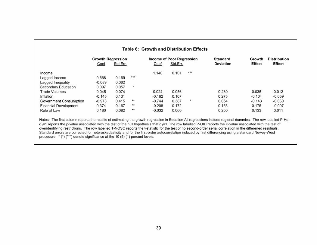
39

Table 6: Growth and Distribution Effects

Growth Regression Income of Poor Regression Standard Growth Distribution

Coef Std.Err. Coef Std.Err. Deviation Effect Effect

Income 1.140 0.101 ***Lagged Income 0.668 0.169 ***Lagged Inequality -0.089 0.062Secondary Education 0.097 0.057 *Trade Volumes 0.045 0.074 0.024 0.056 0.280 0.035 0.012Inflation -0.145 0.131 -0.162 0.107 0.275 -0.104 -0.059Government Consumption -0.973 0.415 ** -0.744 0.387 * 0.054 -0.143 -0.060Financial Development 0.374 0.167 ** -0.208 0.172 0.153 0.175 -0.007Rule of Law 0.180 0.082 ** -0.032 0.060 0.250 0.133 0.011

Notes: The first column reports the results of estimating the growth regression in Equation All regressions include regional dummies. The row labelled P-Ho: α1=1 reports the p-value associated with the test of the null hypothesis that α1=1. The row labelled P-OID reports the P-value associated with the test of overidentifying restrictions. The row labelled T-NOSC reports the t-statistic for the test of no second-order serial correlation in the differened residuals. Standard errors are corrected for heteroskedasticity and for the first-order autocorrelation induced by first differencing using a standard Newey-West procedure. * (*) (***) denote significance at the 10 (5) (1) percent levels.

40

Table 7: Openness and Incomes of the Poor

Trade Adjusted Trade Sachs-Warner Import Taxes Dummy for Dummy for

Volumes Volumes Trade Policy Index As Share of Imports WTO Membership Capital ControlsCoef Std.Err. Coef Std.Err. Coef Std.Err. Coef Std.Err. Coef Std.Err. Coef Std.Err.

Basicln(Per Capita GDP) 1.094 0.108 *** 1.047 0.133 *** 1.077 0.092 *** 0.936 0.136 *** 0.917 0.104 *** 0.869 0.116 ***Openness Measure -0.039 0.088 -0.038 0.167 -0.071 0.065 -0.161 0.358 0.021 0.043 -0.090 0.051 *

P-Ho: α1=1 0.386 0.724 0.407 0.638 0.428 0.259P-OID 0.257 0.135 0.431 0.074 0.425 0.183T-NOSC -0.751 -0.767 -0.677 1.263 -0.998 -1.084# Observations 223 213 234 137 269 208

Interaction with Per Capita GDPln(Per Capita GDP) 1.102 0.092 *** 0.991 0.126 *** 1.066 0.076 *** 1.013 0.082 *** 1.012 0.078 *** 0.969 0.084 ***Openness Measure -0.323 1.363 1.188 1.601 0.237 0.573 0.604 3.133 -0.026 0.558 -0.515 0.587Openness Measure x ln(Per Capita GDP) 0.030 0.146 -0.123 0.169 -0.036 0.072 -0.085 0.396 0.002 0.070 0.052 0.064

P-Ho: α1=1 0.267 0.942 0.386 0.873 0.876 0.708P-OID 0.218 0.144 0.567 0.126 0.226 0.121T-NOSC -0.742 -0.816 -0.696 1.253 -0.905 -1.005# Observations 223 213 234 137 269 208

Interaction with Per Capita GDP and Land

ln(Per Capita GDP) 1.120 0.105 *** 0.901 0.099 *** 1.046 0.084 *** 1.063 0.083 *** 1.101 0.072 *** 1.009 0.081 ***Openness Measure 0.304 1.780 1.161 1.485 0.109 0.605 2.552 2.858 0.513 0.569 -0.574 0.607ln(Arable Land/Worker) -0.090 0.031 *** -0.086 0.023 *** -0.018 0.032 -0.037 0.029 -0.054 0.039 -0.038 0.025Openness Measure x ln(Per Capita GDP) -0.036 0.198 -0.074 0.170 -0.024 0.075 -0.378 0.385 -0.066 0.072 0.050 0.066Openness Measure x ln(Arable Land Per Worker) 0.061 0.070 0.245 0.111 ** -0.041 0.035 -0.366 0.262 0.016 0.039 -0.023 0.031

P-Ho: α1=1 0.253 0.322 0.582 0.443 0.163 0.915P-OID 0.030 0.062 0.267 0.082 0.208 0.095T-NOSC -0.755 -0.896 -1.134 0.421 -1.019 -1.492# Observations 207 207 219 131 243 193 Notes: All regressions include regional dummies. The row labelled P-Ho: α1=1 reports the p-value associated with the test of the null hypothesis that α1=1. The row labelled P-OID reports the P-value associated with the test of overidentifying restrictions. The row labelled T-NOSC reports the t-statistic for the test of no second-order serial correlation in the differened residuals. Standard errors are corrected for heteroskedasticity and for the first-order autocorrelation induced by first differencing using a standard Newey-West procedure. * (*) (***) denote significance at the 10 (5) (1) percent levels.

41

Table 8: Other Determinants of Incomes of the Poor

Years Primary Social Agricultural Voice Voice with

Education Spending Productivity Macro ControlsCoef Std.Err. Coef Std.Err. Coef Std.Err. Coef Std.Err. Coef Std.Err.

ln(Per Capita GDP) 1.067 0.088 *** 1.025 0.101 *** 0.985 0.104 *** 0.933 0.095 *** 1.117 0.098 ***

Years Primary Education 0.014 0.031

Government Consumption/ -1.553 0.547 ***GDP

Social Spending -0.664 0.429/Total Public Spending

Agricultural Relative 0.060 0.081Productivity

Voice 0.095 0.053 * 0.029 0.058

P-Ho: α1=1 0.448 0.803 0.886 0.480 0.233P-OID 0.213 0.028 0.166 0.302 0.419T-NOSC -0.384 0.594 -0.837 -0.970 -0.767# Observations 222 111 197 265 207

Notes: All regressions include regional dummies. The row labelled P-Ho: α1=1 reports the p-value associated with the test of the null hypothesis that α1=1. The row labelled P-OID reports the P-value associated with the test of overidentifying restrictions. The row labelled T-NOSC reports the t-statistic for the test of no second-order serial correlation in the differened residuals. Standard errors are corrected for heteroskedasticity and for the first-order autocorrelation induced by first differencing using a standard Newey-West procedure. * (*) (***) denote significance at the 10 (5) (1) percent levels.

42

Figure 1: Incomes of the Poor and Average Incomes

Levels

y = 1.0734x - 1.7687R2 = 0.8846

3

4

5

6

7

8

9

10

3 4 5 6 7 8 9 10Log(Per Capita Income)

Log(

Per C

apita

Inco

me

in P

oore

st Q

uint

ile)

Growth Rates

y = 1.185x - 0.0068R2 = 0.4935

-0.2

-0.15

-0.1

-0.05

0

0.05

0.1

0.15

0.2

-0.2 -0.15 -0.1 -0.05 0 0.05 0.1 0.15 0.2

Average Annual Change in log(Per Capita Income)

Ave

rage

Ann

ual C

hang

e in

log(

Per C

apita

Inco

me

in P

oore

st

Qui

ntile

)

43

Figure 2: Growth and Distribution Effects of Policies

-25% -20% -15% -10% -5% 0% 5% 10% 15% 20%

Trade Volumes

Inflation

GovernmentConsumption

FinancialDevelopment

Rule of Law

Percent of Per Capita GDP

GrowthDistribution