growth in indonesia’s manufacturing sectors:...

GROWTH IN INDONESIA’S MANUFACTURING SECTORS:

URBAN AND LOCALIZATION CONTRIBUTIONS

Jennifer Day

Lecturer in Urban Planning

Faculty of Architecture, Building, and Planning

The University of Melbourne

[email protected]

Peter Ellis

Lead Urban Economist

South Asia Region

The World Bank

[email protected]

Summary: This paper examines the factors influencing the growth of four dominant and

growing manufacturing sectors in Indonesia. The main purpose of this paper is to

discriminate between localization economies and urbanization processes, and their

contributions to growth in selected manufacturing sectors in Indonesia. A secondary purpose

is to identify the characteristics of local places that facilitate or hinder economic growth in

the manufacturing sectors. We conclude that the studied manufacturing sectors benefit from

localization economies, but that urbanization is largely not a contributor to growth in

manufacturing. This suggests that new and geographically-isolated growth poles are

probably not a viable growth option for Indonesia’s manufacturing sector. Rather, decreasing

the economic distance between vertically and horizontally-linked firms would be more

conducive to growth.

Key Words: Localization, urbanization, manufacturing, Indonesia, desakota, kotadesasi

Sixth Urban Research and Knowledge Symposium 2012

2

I. INTRODUCTION

This paper examines the factors influencing the growth of four dominant and growing

manufacturing sectors in Indonesia. The main purpose of this paper is to discriminate

between the urban contribution to manufacturing growth, and localization economies in

selected manufacturing sectors in Indonesia. A secondary purpose is to examine conditions

that facilitate economic growth in Indonesian kabupaten and kota manufacturing activity –

that is, to identify the characteristics of local places that facilitate or hinder economic growth

in the manufacturing sectors.

Recent work on Indonesia concludes that the country has failed to leverage the strength of its

urbanization to generate economic returns (WB, 2012). Compared to its neighbors in Asia,

Indonesia has been sluggish in accruing Gross Domestic Product (GDP) growth that is

commensurate with its urbanization rates (WB, 2012). We focus on the impacts of

localization economies and urbanization, in addition to variables reflecting human capital,

infrastructure investments, economic activity in the district, and capital. Our core interest is

in understanding how the processes of urbanization and localization contribute to economic

development.

The benefits of localization economies and urbanization are currently in the forefront of

public policy debates in Indonesia. Some policy makers and advisors advocate rural-centric

growth policies that neglect urban regions. Others are pushing for establishment of isolated

growth poles placed in eastern Indonesia, to stimulate growth in lagging regions.

As stated above, our core inquiry here is whether urban regions contribute significantly to

development in the manufacturing sectors, and also whether localization effects are major

contributors to growth. We stop short of labeling our study as one of urbanization economies

in the sense that Jacobs (Jacobs, 1969) intended, i.e., economic diversity in a region. Our

literature review (in the Background and Approach sections below) will sample from the

literature that takes this approach, but will describe how our indicators reflect more-nuanced

urbanization processes. To avoid confusion, we describe our inquiry as a study into

localization economies and urbanization, rather than of urbanization and localization

economies.

We conclude that the studied manufacturing sectors benefit from localization economies, but

that urbanization externalities are largely not present. In combination with other findings

indicating that state-owned enterprise suppresses growth, this suggests that new and

geographically-isolated growth poles are probably not a viable growth option for Indonesia’s

manufacturing sector. Rather, decreasing the economic distance between vertically and

horizontally-linked firms would be more conducive to growth.

II. BACKGROUND

Although we do not classify this study as one examining urbanization economies and

localization economies (we classify it instead as one studying localization economies and

urbanization), it is instructive to review the concepts of urbanization and localization

externalities and the findings related to them. At the end of this section, we outline how we

improve upon the existing formulations of urbanization for this study’s particular needs, and

in Section III, we detail our choice of method and indicators.


3

Urbanization and localization economies are two types of scale economies that can act on

manufacturing sectors. Localization economies – efficiencies resulting from the clustering of

like firms – are more recently also called Marshall-Arrow-Romer (MAR) externalities

(Arrow, 1962; Marshall, 1920; Romer, 1986). Urbanization economies, or more-recently

Jacobs externalities (Jacobs, 1969), are efficiencies resulting from the clustering of firms and

people into diverse agglomerations (Beardsell & Henderson, 1999; Fan & Scott, 2003).

The concept of urbanization economies has been operationalized both in terms of diversity of

economic activity, and as the size of an urban agglomeration (Rosenthal & Strange, 2003). A

number of notable studies measure urbanization economies in relation to the urban size rather

than a diversity of industries. For instance, Nakamura (Nakamura, 1985) examines sub-

national determinants of urban agglomeration economies for Japanese cities cross-sectionally,

in 1979. He includes localization economies (measured in terms of industry employment)

and urbanization economies (measured in terms of total urban population). Nakamura finds

evidence for both urbanization and localization economies (productivity elasticities of 4.5

and 3.4 percent, respectively), and further concludes that light industries benefit more from

urbanization economies than localization economies, and vice versa for heavy industries. In a

cross-sectional study of two-digit industrial activity in cities of Brazil and the United States,

Henderson (1986) proxies urbanization effects with both total city employment and total city

population, with similar results. He finds localization effects in the USA and Brazil, but few

localization effects. Since our interest is in the influence of cities and urbanization on growth,

we will use a measure of urbanization economies that reflects population rather than

industrial diversity.

The distinction between urbanization and localization economies is important in planning for

growth in manufacturing sectors, in both urban and non-urban areas. The two types of scale

economies have different effects on agglomeration economies. These effects may occur

together. If an industry is subject primarily to localization economies, it will not benefit from

the diversity of activities usually found in large metropolitan areas. Rather, that industry’s

growth will be enhanced in specialized clusters of similar or complementary activity, usually

found in smaller urban agglomerations (J. Vernon Henderson, 2003). Location in specialized

clusters allows firms to benefit from positive externalities of scale such as transportation

costs, while saving on the diseconomies of agglomeration such as high congestion and high

land rents. Standardized industries such as textiles and wood processing, then, tend to locate

in smaller, more-specialized areas (Black & Henderson, 2002)

On the other hand, if urbanization economies are the predominant driving force in an

industry’s success, that industry will thrive in more economically-diverse regions. This type

of activity includes fashion, publishing, and FIRE (finance, insurance, and real estate) (J.

Vernon Henderson, 2003). These more-diverse regions also tend to be larger metropolitan

areas (Kolko, 1999).

Duranton and Puga (1999) formalize the relationship between urbanization and localization

economies from an industry life-cycle perspective. They demonstrate that industries in the

innovative early phases of development tend to locate in large, diverse metropolitan regions.

As their functions become standardized, they relocate to smaller, more-specialized areas to

take advantage of scale economies and to avoid agglomeration diseconomies.

Many analysts have noted that innovation occurs in clusters in the United States (Feldman,

1994), Europe (Breshchi, 1999; Cäniels, 1999), Japan, and other developed nations. The


4

relative importance of urbanization and localization in economic development is the subject

of an extensive and long-running discussion in economics, with many researchers searching

for an explanation of the drivers and benefits of clustering (Combes, 2000; Harrison, Kelley,

& Gant, 1996; Porter, 2003).

There is a well-established and diverse literature examining the specific nature and sources of

local scale externalities. The so-called micro foundations of local scale externalities are

reviewed extensively Duranton and Puga (2004) and summarized in Rosenthall and Strange

(2003). Rosenthall and Strange conclude that the literature provides evidence for all of

Marshall’s (1920) proposed micro-sources: input sharing by firms (resulting in increasing

returns to scale), labor pooling (providing a larger labor pool, thus reducing risks to both

employees and firms), and knowledge spillovers (where firms and individuals learn from

each other). They additionally note that recent literature provides evidence for non-

Marshallian sources of local economies of scale, such as rent-seeking, natural advantage, and

home-market effects, and opportunities for urban residents to consume a more-diverse set of

goods and services. Our study does not allow for much comment on these micro foundations

in Indonesia,

Rosenthall and Strange also summarize the literature by concluding that there are three

dimensions of the scope of local scale economies, which are developed in the literature.

These are industrial, geographic, and temporal. The industrial scope includes localization

economies. Geographic scope includes the interaction over space of firms and regions.

Rosenthall and Strange conclude that all of these scopes attenuate with distance. Our study

examines all three of these scopes. We examine the effects of geographic spillovers by

including the influence of neighbors in our measure of localization economies (discussed in

detail in Section III). Temporal effects refer to the idea that it may not only be current

features of the local economy that influence production; past events could also influence

current economic output (2003). Henderson (2003) and Glaeser (1992) point out that

temporal effects can take different forms. One effect is longer-term, involving a build-up of

local industry knowledge and expertise that occurs over time. The other type of temporal

effect happens in the form of “experiments” with more immediate results. This could include

immediate benefits (such as productivity increases resulting from changing suppliers) that

occurred in the past. Henderson points out that it is difficult to distinguish these two types of

temporal effects, but that we can determine whether lagged effects in general occur.

We leave a detailed discussion of the mechanisms by which local scale economies occur –

labor pooling, shared suppliers, knowledge spillovers, rent-seeking, etc. – to the many

excellent literature reviews on the subject (Beaudry & Schiffauerova, 2009; Davis &

Henderson, 2003; G. Duranton & Puga, 2004; Rosenthal & Strange, 2003). Our analysis

focuses urbanization and localization effects on manufacturing growth in Indonesia,

regardless of their origins. Despite a rich theoretical literature (Fujita & Krugman, 1995;

Krugman, 1991a, 1991b, 2007) and a large body of empirical work in developed nations

(Barro & Sala-i-Martin, 1991a; Beardsell & Henderson, 1999; Ellison & Glaeser, 1997,

1999; Mukkala, 2003), little analysis focuses on Indonesia. Given its large and diverse

population spread over more than 17,000 islands and with large spatial disparities in

infrastructure, accessibility, and incomes, we think Indonesia provides a good case study of

sub-national drivers of growth. This review of the literature demonstrates the dearth of

studies that address Indonesia’s manufacturing growth outcomes.


5

Most of the existing studies on Indonesia that address the roles of urbanization or localization

effects focus on one or the other. McCulloch and Sjahrir (2008) use a weighted average of

GRDP growth in neighboring districts as a measure of nearness to a growing region.

However, their study does not include sector-specific localization effects. Deichmann and

Kaiser (2005), working at the kabupaten and kota levels in Indonesia, conclude that

localization economies are important in manufacturing firm-location decisions. Using road

densities as a proxy for accessibility (we believe our metrics are superior), they conclude that

road-infrastructure improvements would do little to draw manufacturing to outlying, lagging

districts in East Kalimantan and South Sulawesi provinces in Eastern Indonesia. Although

they address the issue of regional disparity in firm location, their approach is cross-sectional,

only for 2001. Our study examines change over time in multiple significant periods in

Indonesia’s recent history. Kuncoro and Dowling (2004) examine effects of economic

agglomeration, but only on Java. Our study covers the entire country.

Some studies do examine localization and urbanization effects concurrently, and these – like

our study – focus largely on sector activity. Fan and Scott (2003) find significant economies

of both urbanization and localization in China, with urbanization economies having larger

effects. However, their analysis is at the provincial level, and proxies for both variables –

location quotient and population of the largest city in the province – are less precise than our

metrics, and the analysis focuses on provinces rather than local governments. Because of the

contribution of rent-seeking to the formation of large cities (Ades, 1995), it is possible that

the effects Fan and Scott interpret as urbanization effects are really rent-seeking effects.

Focusing on Java, Indonesia, Henderson and Kuncoro (1996) find localization effects in

textiles, non-metallic minerals, and machinery sectors. They additionally find urbanization in

the wood, furniture, and publishing sectors. Their study is Java-focused on does not include

post-decentralization outcomes. In Korea, Lee and Zang (1998) find evidence of localization

(but not urbanization) economies in nineteen industries. In Korea, Henderson et al (2001)

conclude that there are localization effects in traditional manufacturing sectors such as

machinery, and urbanization effects in knowledge-sharing industries such as the high-tech

sectors (V. Henderson, Lee, & Lee, 2001). In India, Lall et al (2004) find evidence of spatial

concentration in the leather and metals sectors, moderate concentration in food products,

textiles, machinery, and electronics, and no systematic patterns of concentration in chemicals

or paper sectors (Lall, Shalizi, & Deichmann, 2004). Other studies have examined the

positive externalities generated from within specific agglomerations (SCHMITZ & NADVI,

1999; Smyth, 1992; Weijland, 1999).

Most of the above studies ignore spatial factors in the construction of indicators of

agglomeration, instead using metrics such as location quotients (Mukkala, 2003) to measure

economic concentrations. McCulloch and Sjahrir (McCulloch & Sjahrir, 2008; Mukkala,

2003) provides a notable exception to this, including economic activity in adjacent districts as

a predictor. Led by Paul Krugman (Krugman, 1991a, 2007), the New Economic Geography

approach posits that transaction costs that affect trade can be reduced by lessening distances –

a concept that is operationalized in the World Development Report 2009 (WB, 2009) as

“economic distance.” Our analysis pays particular attention to the concept of economic

distance in the formulation of measures for both urbanization and localization economies.

As the passages in this section suggest, analysis of sector growth in Indonesia is at best

outdated, with the latest academic study published in 1996. In addition to providing an

update that includes post-decentralization outcomes, we add to this body of work in a number


6

of ways. First, our metrics for urbanization and localization incorporate the concept of

economic distance (WB, 2009), and do not rely on simple measures such as population of the

largest city or adjacency with a growing region. Second, our formulation of urbanization and

localization externalities allows for a more-realistic representation of Asia’s nuanced

urbanization processes, which will be discussed in the next section. Third, we include

indicators of the quality of infrastructure, which have not been used in previous analyses, and

which are more-direct measures of the phenomena we wish to represent. These include

extensiveness and quality of the road network and the reliability of electric power. Fourth,

we incorporate local economic factors (such as government involvement in industry through

state-owned enterprise and indicators of the “upscaleness” of the local economy). Fifth, we

incorporate measures of the innovative capacity of the manufacturing sectors. The next

section outlines our approach to the analysis, including variables, data, and models.

III. APPROACH

Four manufacturing sub-sectors sectors are analyzed here as case studies: textiles1, electric

machinery2, paper and products

3, and printing and publishing

4. The first three were chosen

because they are both dominant and fast-growing sectors in the Indonesian national economy.

Initially, we were interested in analyzing, separately, two case sectors with high value added

reported in 2006, and two case sectors with fast growth over the 1993-2006 analysis period.

This was to facilitate understanding of the factors that make sectors both large and fast-

growing, and additionally, to identify factors that constrain growth. Interestingly, the

selection process was simplified when our analysis showed that the top fifteen manufacturing

industries in 2006 were also the top fifteen fastest-growing for the 1993-2006 analysis period,

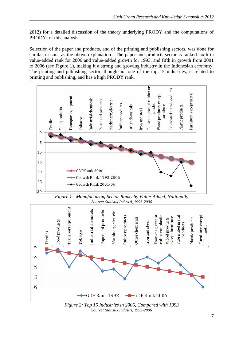
and correspond closely to the fastest-growing sectors for the 2001-06 analysis period. Figure

1 shows the top 15 manufacturing sectors ranked by value-added, the top 15-ranked sectors

by growth of value-added from 1993 to 2006, and the top 15-ranked sectors by value-added

growth from 2001 to 2006.

An additional factor in the selection of textiles, paper and products, and electric machinery

was that both sectors had improved their economic rank from 1993 to 2006. Textiles moved

from third to first place, paper and products moved from twelfth place, and electric

machinery moving from eleventh to seventh place, in terms of its value-added contribution to

the national economy. Figure 2 shows the rank of the top 15 sectors in 2006, and its

corresponding rank in 1993. Both textiles and electric machinery improved their standing in

the national manufacturing economy over the 1993-2006 analysis period – in the case of

electric machinery, the jump in rank was quite significant.

Finally, printing and publishing was chosen as a case sector because of its high PRODY

value. PRODY is an indicator developed by Hausmann et al (2007), which reflects the

upscaleness of an industry. PRODY is based on the presumption that goods and services

produced by richer economies should rank higher on a measure of upscaleness. Thus, a high

PRODY indicates that the sector is relatively upscale in Indonesia’s basket of manufacturing

sectors (R Hausmann et al., 2007). We direct the reader to Appendix B of Ellis et al (WB,

1 The textiles sector corresponds to ISIC (Revision 2) code 321 at the three-digit level. 2 The electric machinery sector corresponds to ISIC (Revision 2) code 383 at the three-digit level. 3 The paper and products sector corresponds to ISIC (Revision 2) code 341 at the three-digit level. 4 The printing and publishing sector corresponds to ISIC (Revision 2) code 342 at the three-digit level.


7

2012) for a detailed discussion of the theory underlying PRODY and the computations of

PRODY for this analysis.

Selection of the paper and products, and of the printing and publishing sectors, was done for

similar reasons as the above explanation. The paper and products sector is ranked sixth in

value-added rank for 2006 and value-added growth for 1993, and fifth in growth from 2001

to 2006 (see Figure 1), making it a strong and growing industry in the Indonesian economy.

The printing and publishing sector, though not one of the top 15 industries, is related to

printing and publishing, and has a high PRODY rank.

Figure 1: Manufacturing Sector Ranks by Value-Added, Nationally

Source: Statistik Industri, 1993-2006

Figure 2: Top 15 Industries in 2006, Compared with 1993

Source: Statistik Industri, 1993-2006


8

IV. MODELS AND DATA

4.1 Model

For robustness, we generate and analyze two sets of models in examining growth impacts,

between 1993 and 2006. One complexity arising from comparisons of data over time is the

large number of new districts that have been created as a result of decentralization. At the

time of decentralization in 1999, there were 292 districts and five additional districts

comprising Jakarta. The number of districts rose to just under 500 by 2009. Fortunately,

districts were largely formed by splitting an existing district into two or more new districts,

so it was fairly easy to collapse the data to pre-Big Bang spatial units. We follow McCulloch

and Sjahrir (2008) in collapsing the data to the 292 pre-Big Bang districts, so that they can be

compared over time.

First, we use fixed effects models to examine the entire time period from 1993 to 2006. This

model allows us to exploit the panel nature of our data, and allows us to control for

unmeasured district-level regulatory factors (e.g., local regulatory environment, business

friendliness), talent (e.g., entrepreneurial ability) and other time-invariant factors for which

we do not have sufficient data (Allison; Greene, 2007). Fixed effects also allow us to control

for selectivity, an issue that will be discussed below in the section titled “Exogenous

Covariates.” We use the logarithm of sector value added (not per capita value-added) as the

dependent variable.

Our models use absolute (not per capita) growth in both the dependent variables and the

independent variable that indicates initial industry size. We choose this approach, rather than

scaling the sector output to the size of the population by using value-added per capita or per

worker, because we are concerned with the growth of the sector – not necessarily the income

per worker. We control for the initial size of the industry in the models using initial sector

value-added.

We also want to analyze effects in different time periods; particularly, pre-decentralization,

during the Asian Financial Crisis of the late 1990s, and after decentralization. Since fixed-

effects models require sufficiently-long time periods to allow for variation (J. Vernon

Henderson, 2003), another model is needed for the shorter time periods. Growth in a district,

over three analysis periods, was modeled using various predictor variables in Cross-Area

Panel Growth Regression (CAPGR). The analysis periods are: 1993-96, 1996-99, and 2002-

06. The 1996-1999 period analysis period isolates the effects of the Asian Financial Crisis.

2000 and 2001 are not included in the analysis because of some data irregularities that we

presume are associated with the Big Bang transition. We discuss these irregularities below.

This second model is a variation of Barro’s (1991a) Cross Country Panel Growth Regression

(CCPGR) models, which uses Ordinary Least Squares (OLS) estimations to model GDP

growth over a period of time against the logarithm of initial GDP and other explanatory

factors. Barro and others, e.g., Hausmann et al (2008), have applied the CCPGR models to

national economies. We apply their model at a sub-national level in Indonesia. Generally,

our model specification is as follows:

gy,i = i + log(yi,0) +

i,0 + i

where


9

is a constant

gy,i is the nominal growth of GRDP over the time period (not GRDP per capita)

y0 is the initial level of GRDP by industrial sector (not GRDP per capita)

X is a matrix of explanatory factors at the beginning of the analysis period

i is an error term

is a coefficient to be estimated, and

is a vector of coefficients to be estimated.

We note that we do not explicitly include that initial sector value-added in our model, as our

measure of localization economies (discussed in the proceeding section) includes own-district

initial sector value-added. Henderson (2003) uses a similar approach, controlling for

temporal and plant-level fixed effects in a study of American manufacturing activity at the

two-digit level. This approach controls for unobserved time-invariant endowments or

location factors that might have influenced firms to locate in a particular district, usefully

controlling for selectivity effects (J. Vernon Henderson, 2003).

4.2 Localization Economies and Urbanization

Urbanization and localization economies are approximated using gravity indices that

represent their position relative to major population centers and sector-specific industrial

concentrations. This section discusses why we believe this approach to be an improvement

over previous indicators for urbanization economies.

Jacobs externalities, or localization economies, refer specifically to the externalities resulting

from diverse economic compositions, and not to urban proximity per se (Beaudry &

Schiffauerova, 2009; Jacobs, 1969). In the literature on manufacturing growth, studies

typically measure urbanization in one of two ways: using a measure of local industrial

variation such as Gini coefficients or variants of the Hirschman-Herfindahl index, and using a

measure of urban population size or urban proximity as a proxy for industrial variation

(Beaudry & Schiffauerova, 2009). Since we are interested in the process of urbanization and

not variation in industrial make-up, we choose a method that reflects both the urbanized

population, and not a measure of industrial variation. Furthermore, we feel that traditional

studies of urbanization economies fail to account for critical aspects of the Asian urbanization

experience – namely Kotadesasi (described in the next paragraph) – and we thus introduce an

indicator here that is designed to reflect a higher level of complexity than standard diversity

indicators permit.

Our definition of urbanization economies honors McGee’s widely-cited concept of Kotadesasi,

often shortened to Desakota (McGee, 1969). Derived from the Indonesian words for city

(kota), village (desa), and process (si), these terms describe the process of urbanization in

Asia as an evolving continuum of urbanization, rather than a simple distinction between

urban and rural. McGee observes that Asia’s cities are surrounded by hinterlands that

interact with the city core at varying degrees depending on spatial proximity and other factors.

To McGee, then, cities and their rural surrounds are socially and economically intertwined,

and so dichotomous urban/rural distinctions are arbitrary and not helpful in describing the

process of urbanization in Asia. We agree, and use the measure of urbanization described

below to allow for this complexity to be reflected in our analysis.

Some studies using the population-based formulation of urbanization have considered only

population or distance, but not both. For instance, Fan and Scott (2003) use population of

largest city in the province in a provincial-level study of agglomeration in China. Deichmann


10

and Kaiser (Deichmann et al., 2005) use road density and travel time measure access to

markets and population centers. McCulloch and Sjahrir (2008) use a weighted average of

GRDP growth in neighboring districts. Our analysis takes this further, employing a gravity

index that considers distance and weight. Unlike these simpler measures, a gravity index

provides a measure of the proximity of a place to regional attractions, weighted by the

distance that must be traversed to reach those attractions. Thus, it reflects “economic

distance” (WB, 2009), or “market potential” (CITATION). Unlike measures that reflect

accessibility to one urban concentration, the gravity index also captures the effects of smaller

urban agglomerations that may be in close proximity but not adjacent. The general formula

for a gravity index is as follows:

GIi = j [ATTRACTIONj]

EDij

where

i denotes a spatial area (in our case, a district)

j denotes an attraction (in our case, metropolitan and economic centers)

GIi is the gravity index for a given district

ATTRACTIONi = denotes the attractive force of a population or economic center

is a analyst-defined decay coefficient, which we assume to be one

EDij is a measure of economic distance, e.g., time or physical distance between origin i and

destination j (in our analysis, travel time)

Higher gravity indices denote higher levels of accessibility to the attracting areas. We use

this principle to develop two sets of gravity indices:

1) Market gravity to proxy urbanization economies (ATTRACTION = population)

2) Sector economic gravity to proxy localization economies (ATTRACTION = sector

value-added)

One beneficial side-effect of this specification for localization economies, is that it serves a

dual purpose of telling us about localization effects, and correcting for spatial autocorrelation.

We note the presence of spatial autocorrelation in the manufacturing GRDP data, detected

using the Moran’s I test5). This means that there is a spatial relationship between the GRDP

of a district and its neighbors’ GRDP. We further note that our gravity index for growth of

manufacturing GRDP (described below) corrects for this potential spatial bias in both the

fixed effects and the CAPGR models, by controlling for the effect of neighbors’ economic

performance on economic performance of a district. Correcting for spatial autocorrelation is

important because its presence can affect parameter estimates, standard errors, and parameter

stability (Pace & Gilley, 1997).

By far the most common ways to measure localization economies in the literature has been to

use location quotients and own-industry employment. Beaudry and Schiffauerova (2009)

find that around 75 percent of studies involving Marshall externalities uses one of these

indicators. Our approach to measuring localization economies extends this concept,

accounting both own-district value added and the value-added of neighboring districts. This

is important because our tests for spatial autocorrelation indicates the presence of spillover

5 For all case sectors, spatial autocorrelation is statistically significant in all years, with Moran Indices of between 0.07 and 0.23 (Moran’s Index varies from -1 to 1, with -1 and 1 representing perfect correlation, and zero representing no correlation).


11

effects, or positive externalities resulting from nearness in space (Baumont, Ertur, & Gallo,

2001; Fingleton & López-Bazo, 2006; J. Vernon Henderson & Kuncoro, 1996; Perret, 2011;

Wardaya & Landiyanto, 2005). Our gravity-based measure, which scales the influence of

neighbors by the separation between them and the home district, is superior to an adjacency-

based approach used by some authors – for instance, (McCulloch & Sjahrir, 2008) – in that it

does not assume reciprocal spillover effects between two regions, but rather, allows for

uneven effects between districts (Perret, 2011).

Sector growth in terms of value-added is taken from the Statistik Industri (Large and

Medium-Scale Manufacturing Census; SI) from 1993 to 2006. We use ISIC Revision 2

classifications at the three-digit level, in order that all data can be commonly represented in

all time periods.

4.3 Endogenous Covariates

Endogeneity can be a problem in growth models, and particularly those related to

urbanization processes, since many processes of urbanization and growth are jointly

determined. For instance, growth can attract population in the form of migration, but the

addition of people to a city can improve GRDP per capita through agglomeration forces. We

build a number of measures into our models to control for potential joint determination

between the dependent and independent variables in the models.

The first set of models, those using fixed effects, are the final result of careful consideration.

Lacking the strictly exogenous instruments required by two-stage least squares estimation,

we follow Henderson (2003) and attempt to control for joint determination of population and

value-added growth (and also education levels and value-aded growth) using the Generalized

Method of Moments (GMM). This method uses lagged levels and lagged growth as

instruments, under the presumption that these predetermined values are correlated with their

future values (J. Vernon Henderson, 2003). However, GMM and fixed-effects estimates

were not qualitatively different, so we report only the fixed-effects results here.

Another benefit of fixed-effects models that is not shared by GMM estimations, is that they

can control for selectivity. Because firms are not randomly assigned to districts, but rather

may choose to locate in a particular district to take advantage of local resources such as labor

or infrastructure, selectivity effects can arise in growth models. Fixed effects models can

control for selectivity (J. Vernon Henderson, 2003), in that they control for unobserved, time-

invariant factors that induce firms to locate in a particular district.

Finally, we note that there could be interaction effects related to spatial proximity in the

fixed-effects models, e.g., infrastructure stock improvements could have different effects in

districts close to major metropolitan areas, versus those further away. The inclusion of

interaction variables do not qualitatively change any variables. Though they are reported

along with the fixed-effects models in Table 2 for the sake of illustration, for the fixed-effects

models, our discussion focuses on Models 1 through 4. We conclude based on the negligible

contributions of GMM and interactions to improve the estimates, that our fixed-effects

models are relatively robust to endogeneity.

For the CAPGR models, using absolute value-added rather than a scaled metric has the added

benefit of eliminating the possibility of lagged feedback between population0 (population at

the start of the analysis period) and value-added growth, in turn eliminating endogeneity


12

effects and simultaneity bias in the models. Figure 3a illustrates the conceptual relationship

between population0, value-added growth over the analysis period, lagged value-added

growth, and value-added0 (value-added at the beginning of the analysis period; district self-

influence is incorporated into the localization metric). Our inquiry is into whether population

levels influence growth in value-added for a given sector. Presumably, larger populations

can have only a positive effect on change in value-added, because larger populations put no

downward pressure on value-added like they do on value-added per capita, i.e., larger

populations do not dilute the benefits of increased value-added. Because of temporal

primacy, value-added growth can have no effect on population0. It is possible that lagged

feedback could occur (shown by the red hashed line, which denotes correlation, but not a

causal direction). Lagged feedback could introduce negative effects between value-added

growth and population0 through the intermediated variable lagged value-added growth.

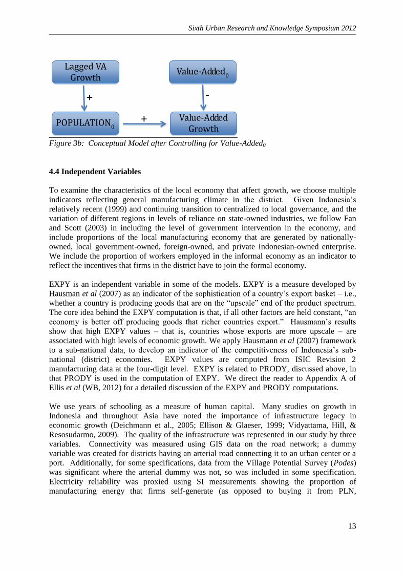
However, we control for this possibility of lagged feedback by adding the variable value-

added0 to the model (shown in Figure 3b). Standard economic theory suggests that the

relationship between value-added0 and value-added growth would be negative, as the figure

shows. However, this does not affect population0.

It is necessary to consider the possibility of joint determination between growth in value-

added and population. Given our panel growth model structures (value-added growth

examined against control variables at the beginning of a three-year analysis period), such

endogeneity would be the result of a lagged feedback effect, i.e., lagged value-added growth

being correlated with population levels in a given initial year of an analysis period. We also

note that increases in lagged value-added growth would positively influence population levels

in the district and surrounding areas (since better-performing industries attract more

prospective workers). Since our models do not control for lagged value-added growth, there

is a possibility of an upward bias on population from this unobserved effect, and thus an

indirect upward bias on value-added growth over the analysis period. Thus, if we were to

observe in our estimations a positive relationship between population0 and value-added

growth, we could not know whether this relationship was due to lagged feedback effects or

presence of urbanization economies.

In short, the direction of the bias due to this endogenous effect would be positive. As we will

see in Table 2, our estimations show little evidence of urbanization economies – even with

the possible bias introduced from lagged feedback effects. Thus, this bias is not problematic

in our models.

Figure 3a: Conceptual Model before Controlling for Value-Added0

POPULATION0 Value-Added

Growth

+

Lagged VA Growth

+ -


13

Figure 3b: Conceptual Model after Controlling for Value-Added0

4.4 Independent Variables

To examine the characteristics of the local economy that affect growth, we choose multiple

indicators reflecting general manufacturing climate in the district. Given Indonesia’s

relatively recent (1999) and continuing transition to centralized to local governance, and the

variation of different regions in levels of reliance on state-owned industries, we follow Fan

and Scott (2003) in including the level of government intervention in the economy, and

include proportions of the local manufacturing economy that are generated by nationally-

owned, local government-owned, foreign-owned, and private Indonesian-owned enterprise.

We include the proportion of workers employed in the informal economy as an indicator to

reflect the incentives that firms in the district have to join the formal economy.

EXPY is an independent variable in some of the models. EXPY is a measure developed by

Hausman et al (2007) as an indicator of the sophistication of a country’s export basket – i.e.,

whether a country is producing goods that are on the “upscale” end of the product spectrum.

The core idea behind the EXPY computation is that, if all other factors are held constant, “an

economy is better off producing goods that richer countries export.” Hausmann’s results

show that high EXPY values – that is, countries whose exports are more upscale – are

associated with high levels of economic growth. We apply Hausmann et al (2007) framework

to a sub-national data, to develop an indicator of the competitiveness of Indonesia’s sub-

national (district) economies. EXPY values are computed from ISIC Revision 2

manufacturing data at the four-digit level. EXPY is related to PRODY, discussed above, in

that PRODY is used in the computation of EXPY. We direct the reader to Appendix A of

Ellis et al (WB, 2012) for a detailed discussion of the EXPY and PRODY computations.

We use years of schooling as a measure of human capital. Many studies on growth in

Indonesia and throughout Asia have noted the importance of infrastructure legacy in

economic growth (Deichmann et al., 2005; Ellison & Glaeser, 1999; Vidyattama, Hill, &

Resosudarmo, 2009). The quality of the infrastructure was represented in our study by three

variables. Connectivity was measured using GIS data on the road network; a dummy

variable was created for districts having an arterial road connecting it to an urban center or a

port. Additionally, for some specifications, data from the Village Potential Survey (Podes)

was significant where the arterial dummy was not, so was included in some specification.

Electricity reliability was proxied using SI measurements showing the proportion of

manufacturing energy that firms self-generate (as opposed to buying it from PLN,

POPULATION0 Value-Added

Growth

+

Lagged VA Growth

Value-Added0

- +


14

Indonesia’s state-owned electricity company)6. As an approximation for capital, we use the

proportion of manufacturing value-added that is dedicated to the servicing of loans, also from

SI. Although this is a less-ideal indicator than the capital-to-labor ratio (K/L), we were

precluded from using K/L because our dataset was missing capital values for some years.

We also interact the loan-interest variable with a term indicating that the district is “lagging”,

i.e., has mean income in the lower 50th

percentile of districts in Indonesia. We do this

because of the great disparity in this variable’s impact in lagging and non-lagging districts.

V. Findings

Table 1 shows the number of districts reporting activity in each manufacturing sector, by year.

Table 2 shows the regression outputs for the final models. Insignificant variables were

allowed to remain if they were of theoretical significance, or if they were significant for the

same dependent variable but in a different analysis period. It is noteworthy that the

dependent variables in Table 3 are different than those in Table 2. In Table 2, the dependent

variables are formulated in terms of logarithms, while in Table 3, they are given as GRDP

growth (x1,000,000). This is because some of the values in Table 3 are negative, due to

negative growth, so a logarithmic formulation is not appropriate here (the log of a negative

number is undefined).

Another important note on interpreting the output of the fixed-effects versus the CAPGR

models, is that they do not explain the same processes. Fixed-effects models can be

interpreted as reflecting levels of variables, or alternately, as a difference-in-difference effect,

where changes in an independent variable are associated with changes in the dependent

variable). By contrast, the CAPGR models provide a growth response associated with initial

levels of a given independent variable.

One worry was that the gravity indices used to measure urbanization and localization

economies would be correlated. For all sectors, however, there was no significant correlation

between the metrics used to proxy for urbanization and localization (correlations ranged from

one to seven percent, without statistical significance). Thus, we conclude that our metrics for

urbanization and localization actually measure different underlying effects.

By far, the most consistently-significant predictor of growth in a district’s manufacturing

industries is localization economies – that is, a district’s economic gravity to other districts

with activity in the same industry. In the fixed-effects models, all of the models show

significant and positive coefficients on this variable, indicating that places with more

accessibility to industrial activity in a sector, have on average higher levels of activity in that

sector. For the CAPGR models, the results are similar, though they vary somewhat between

time periods. In the 1993-96 and 2002-06 analysis periods, seven of the eight equations

show this as a significant and positive predictor, and the eighth (Model 19) is just on the

verge of significance.

In the 1996-99 period, during the Asian Financial Crisis, the pattern described above does not

hold – that is, localization economies do not (except in the case of the textiles sector) appear

6 Perusahaan Listrik Negara


15

to help or hinder growth7. In this period, all of the sectors declined, so the coefficients are

perhaps better interpreted as whether they were related to slowed (positive sign) or increased

(negative sign) decline. Only in the textiles sector does an impact of localization appear, with

positive effects. Other factors matter more in recession – namely, EXPY (districts producing

more upscale products in general saw slower decline in the Paper and Products sector),

informal economic activity (districts with a higher share of informal workers saw larger

declines in the Paper and Products sector), and connectivity.

Regarding urbanization effects, in the fixed-effects models, where urbanization effects are

significant, they are much larger in magnitude than localization effects (the log-log

formulation allows us to compare across variables). This is a significant finding, particularly

for areas outside of metropolitan areas. Although localization affects all industries studied,

urbanization has larger effects where it is significant. In Model 1 (textiles), the market

potential index is verging on significance for the overall variable, and is significant in the

interaction term with non-metro areas. For urban districts, a one-percent increase in

accessibility to population centers is associated with a 2.459 percent increase in textiles

manufacturing GRDP. For non-urban areas, an increase of one percent in accessibility is

associated with a whopping 7.14 (9.473 minus 2.459) percent increase in textiles

manufacturing GRDP. For the electric machinery sector, increased market potential

decreases manufacturing output (as indicated by the negative sign), possibly due to costs of

locating heavy industry near urban centers. However, for non-urban areas, better

accessibility to population centers is associated with higher output. Urbanization effects are

not significant in the paper and printing sectors.

The CAPGR models (Tables 3a and 3b) provide little evidence that urbanization is associated

with growth in the post-decentralization period (2002-2006). However, in the pre-

decentralization analysis periods, there is some evidence suggesting that non-metro paper and

products firms benefitted from proximity to urban centers (1993-96), and that both urban and

rural areas with higher market potential declined more slowly during the crisis than those

further away (1996-99).

These results are interesting. Proximity to other firms making similar products matters more

consistently than any other variable included in the model, but urbanization is far more

influential when it does matter. That spatial proximity to other districts with a manufacturing

presence is the consistently important across industries in determining whether a district will

grow its industry – and that this effect gets stronger with spatial proximity to larger textiles

centers – is not a surprising finding. It is well-established in industrial theory that firms co-

locate in order to actualize agglomeration economies, for instance, sharing suppliers and

access to trained and affordable labor pools. However, even though the result is not

surprising, the presence of the effect indicates that firms attempting to locate away from the

7 We were concerned that our gravity-based indicators for localization economies and urbanization might be measuring the same underlying phenomenon, given that industrial location patterns could vary with the locations of population concentrations. We test the degree to which the two metrics measure the same underlying phenomena using Pearson correlations. We test correlations between market gravity and sector gravity metrics in each of the years 1993, 1996, 1999, 2001, and 2006. We find that of these, the largest observed correlation is -0.0620, with none of the correlation coefficients even approaching significance. Thus, we feel confident that the two variables measure different underlying phenomena.


16

established industrial clusters may not fare as well as those locating near a cluster. Thus,

economic development strategies in Indonesia should exploit the proximity factor.

Table 1: Districts Reporting Sector Manufacturing Activity

Year Textiles Electric

Machinery

Paper and

Products

Printing and

Publishing

1993 101 35 56 63

1994 109 39 55 67

1995 123 42 60 77

1996 125 43 63 84

1997 124 46 63 79

1998 119 42 65 83

1999 197 38 66 74

2000 165 26 52 52

2001 111 11 23 40

2002 179 19 52 60

2003 179 27 55 61

2004 180 28 59 61

2005 201 33 68 86

2006 233 38 76 106 Source: Statistik Industri, 1993-2006


17

Table 2. Value-Added Regressions by Sector, with Fixed Effects, 1993-2006

(1) (2) (3) (4) (5) (6) (7) (8)

VARIABLES Log of

Textiles VA

Log of

Electric

Machinery

VA

Log of Paper

and Products

VA

Log of

Printing and

Publishing

VA

Log of

Textiles VA

Log of

Electric

Machinery

VA

Log of Paper

and Products

VA

Log of

Printing and

Publishing

VA

Interaction Terms Included No No No No Yes Yes Yes Yes

Localization Economies and Urbanization

Log of market potential index (urbanization

economies)

2.459 -4.287*** -1.614 1.693 2.480 -4.112*** -1.032 2.745**

(0.107) (0.000) (0.132) (0.109) (0.143) (0.000) (0.386) (0.019)

Log of market potential index, nonmetro

(interaction term)

9.473*** 6.681*** 1.854 1.605 9.526*** 6.686*** 1.825 1.722

(0.000) (0.000) (0.222) (0.281) (0.000) (0.000) (0.230) (0.248)

Log of sector economic gravity index

(localization economies)

0.409*** 0.335*** 0.370*** 0.377*** 0.408*** 0.335*** 0.370*** 0.376***

(0.000) (0.000) (0.000) (0.000) (0.000) (0.000) (0.000) (0.000)

District Industrial Characteristics

Proportion of mfg. value-added produced

by central-government-owned firms1

0.001 -0.003 -0.002 -0.005 0.000 -0.003 -0.002 -0.006

(0.919) (0.428) (0.698) (0.310) (1.000) (0.428) (0.708) (0.280)


by local-government-owned firms

-0.032*** -0.017*** -0.026*** -0.023*** -0.032*** -0.017*** -0.026*** -0.023***

(0.000) (0.000) (0.000) (0.000) (0.000) (0.000) (0.000) (0.000)


by foreign-owned firms

0.001 -0.004 0.013* -0.011 0.002 -0.004 0.014** -0.013*

(0.883) (0.523) (0.052) (0.102) (0.871) (0.443) (0.049) (0.055)

Log of EXPY -0.198 0.467* -0.364 0.787** -0.288 0.460* -0.372 0.719**

(0.685) (0.091) (0.289) (0.019) (0.559) (0.098) (0.281) (0.034)

Proportion of workers employed in the

informal sectors

-0.104*** -0.061*** -0.037** -0.119*** -0.106*** -0.060*** -0.036** -0.121***

(0.000) (0.000) (0.022) (0.000) (0.000) (0.000) (0.027) (0.000)

Infrastructure Stock

Proportion of manufacturing energy that is

self-generated by the firm

-0.007* -0.001 -0.002 -0.002 -0.006 -0.001 -0.001 -0.000

(0.051) (0.704) (0.455) (0.426) (0.103) (0.724) (0.544) (0.993)

Financial and Human Capital


18

Proportion of manufacturing value-added

dedicated loan servicing

-0.250 0.006 0.251 0.056 -0.968* 0.150 0.430 0.487

(0.272) (0.965) (0.116) (0.720) (0.061) (0.609) (0.237) (0.171)

Average years of schooling for adults older

than 25

1.698 -3.924*** -2.746** -5.212*** 2.083 -3.943*** -2.871** -5.168***

(0.323) (0.000) (0.022) (0.000) (0.227) (0.000) (0.017) (0.000)

Interaction Terms



0.001 -0.000 -0.000 0.000

(0.451) (0.700) (0.458) (0.394)



0.000 -0.001 -0.001* -0.000

(0.936) (0.174) (0.069) (0.483)



0.000 -0.000 0.001 -0.000

(0.939) (0.813) (0.310) (0.616)

Log of EXPY -0.044 0.003 -0.014 -0.069**

(0.362) (0.910) (0.679) (0.036)


informal sectors

-0.000 -0.001 0.001 0.001

(0.926) (0.581) (0.685) (0.826)



-0.000 -0.000 -0.000 -0.001***

(0.314) (0.876) (0.686) (0.001)



0.163 -0.033 -0.039 -0.099

(0.125) (0.582) (0.599) (0.174)


than 25

0.362* -0.091 -0.190 0.056

(0.067) (0.415) (0.171) (0.678)

Constant 23.203*** 7.742* 17.190*** 10.779** 24.067*** 7.803* 17.501*** 11.952**

(0.003) (0.076) (0.002) (0.043) (0.002) (0.076) (0.001) (0.025)

Observations 3,086 3,086 3,086 3,086 3,086 3,086 3,086 3,086

R-squared 0.288 0.185 0.209 0.232 0.290 0.186 0.210 0.237

Number in panel 260 260 260 260 260 260 260 260

p-values in parentheses

*** p<0.01, ** p<0.05, * p<0.1

Dependent variables: Value added by industry (ISIC Revision 2, 3-digit level) 1 Suppressed category: Proportion of manufacturing value-added produced by private Indonesian-owned firms. NOTE: this metric includes all manufacturing value-added, not just

sector-specific values.

Table 3a. Value-Added Regressions by Sector, Cross-Area Panel Growth Models, 1993-1999

(9) (10) (11) (12) (13) (14) (15) (16)


19

VARIABLES Textiles VA

Electric

Machinery

VA

Paper and

Products VA

Printing and

Publishing

VA

Textiles VA

Electric

Machinery

VA

Paper and

Products VA

Printing and

Publishing

VA

Years 1993-1996 1993-1996 1993-1996 1993-1996 1996-1999 1996-1999 1996-1999 1996-1999

Localization Economies and Urbanization

Market potential index (urbanization

economies)

120.040 -102.670 -60.227 8.054 2,015.415 -278.131 937.457** 1,134.679

(0.320) (0.589) (0.125) (0.828) (0.213) (0.877) (0.046) (0.210)

Market potential index, nonmetro areas

(interaction term)

-118.340 102.165 64.611* -7.922 -2,017.866 264.136 -919.760* -1,130.011

(0.329) (0.590) (0.092) (0.830) (0.212) (0.883) (0.050) (0.210)

Sector economic gravity index

(localization economies)

1.477*** 5.593*** 1.741*** 1.402*** 6.301*** 1.055 -0.450 -0.653

(0.000) (0.001) (0.000) (0.000) (0.000) (0.521) (0.384) (0.337)




-7.787** -5.205 -0.230 -0.981 16.215 5.081 -6.406 -23.163

(0.029) (0.440) (0.940) (0.237) (0.598) (0.834) (0.605) (0.294)



1.678 5.221 -5.800 1.252 -30.285 6.820 -27.749 -32.270

(0.625) (0.502) (0.270) (0.450) (0.444) (0.862) (0.284) (0.413)



24.762 32.966 -3.705 5.399* 78.034 247.064* 40.308 20.184

(0.282) (0.159) (0.304) (0.098) (0.235) (0.096) (0.313) (0.345)

Log of EXPY -78.030 -526.216 234.658 287.881 1,003.054 8,476.646 1,871.042 -4,155.921

(0.808) (0.523) (0.457) (0.162) (0.669) (0.121) (0.172) (0.366)


informal sectors

-4.555 19.320* -1.312 -3.895 -40.742 -65.047 -65.771** -75.299

(0.695) (0.060) (0.737) (0.148) (0.503) (0.208) (0.031) (0.342)




-2.731 -3.296 -0.978 -0.005 -8.072 9.851 7.700 -27.521

(0.410) (0.328) (0.478) (0.990) (0.702) (0.500) (0.506) (0.336)




-1,495.845 -1,105.077 -677.244 641.666 -13,991.870 -4,208.430 2,920.952 -22,777.031

(0.358) (0.482) (0.386) (0.333) (0.737) (0.809) (0.668) (0.308)

Average years of schooling for adults

older than 25

-1,041.654 47.747 -70.358 -667.122 -4,243.017 -10,806.341* -

6,697.351*** 884.397

(0.175) (0.945) (0.735) (0.222) (0.484) (0.050) (0.002) (0.572)

Constant 3,545.090 7,215.715 -3,472.205 -3,164.152 -5,919.514 -115,801.605 -14,837.561 73,582.292

(0.522) (0.558) (0.500) (0.168) (0.893) (0.147) (0.500) (0.361)

Observations 231 231 231 231 256 256 256 256

R-squared 0.703 0.733 0.680 0.539 0.831 0.134 0.154 0.030



20

*** p<0.01, ** p<0.05, * p<0.1

Dependent variables: Value added by industry (ISIC Revision 2, 3-digit level) 1

Suppressed category: Proportion of manufacturing value-added produced by private Indonesian-owned

firms. NOTE: this metric includes all manufacturing value-added, not just sector-specific values.


21

Table 3b. Value-Added per capita Regressions by Sector, Cross-Area Panel Growth Models, 2002-2006

(17) (18) (19) (20)

VARIABLES Textiles VA

Electric

Machinery

VA

Paper and

Products VA

Printing and

Publishing

VA

Years 2001-2006 2001-2006 2001-2006 2001-2006

Urbanization and Localization

Economies

Market potential index (urbanization

economies)

1,910.756 155.012 -1,467.270 667.035

(0.277) (0.790) (0.177) (0.123)

Market potential index, nonmetro areas

(interaction term)

-1,913.634 -155.059 1,762.942 -666.658

(0.276) (0.789) (0.114) (0.123)

Sector economic gravity index (localization

economies)

0.888*** 0.932** 2.067 1.995**

(0.001) (0.038) (0.105) (0.011)




114.650 -31.624* -72.896 17.531

(0.180) (0.058) (0.370) (0.478)



71.882 -36.699** -11.326 -9.838

(0.169) (0.039) (0.831) (0.365)



528.974*** -5.635 526.912* -21.262

(0.004) (0.931) (0.052) (0.225)

Log of EXPY 9,676.511* 3,896.024* 2,392.807 962.757

(0.074) (0.072) (0.629) (0.264)


informal sectors

-209.753 9.620 -378.613 0.763

(0.258) (0.902) (0.205) (0.977)




-54.208 -5.893 20.855 -1.143

(0.236) (0.698) (0.741) (0.787)




40,677.538 -5,644.368 15,359.587 -2,381.870

(0.245) (0.275) (0.634) (0.157)


than 25

-34,428.885** -302.735 -30,310.045* 1,485.283

(0.013) (0.932) (0.074) (0.389)

Constant -78,051.109 -58,648.344 38,292.344 -17,588.382

(0.406) (0.131) (0.690) (0.224)

Observations 250 250 250 250

R-squared 0.656 0.527 0.279 0.555


*** p<0.01, ** p<0.05, * p<0.1

Dependent variables: Value added by industry (ISIC Revision 2, 3-digit level) 1 Suppressed category: Proportion of manufacturing value-added produced by private Indonesian-owned

firms. NOTE: this metric includes all manufacturing value-added, not just sector-specific values.


22

Sector activity was mapped in order to examine these proximity effects visually.

Districts with activity in a sector were mapped according by year that the first firm

opened in that district. In Figure 4 through 10 below, dark blue shading indicates that

the district had activity in a given sector prior to 2002. The darkest red shading

indicates that the industry was first established in that district in 2002, and the red

shading lightens as the year textiles were first introduced to the district extends away

from 2002 toward 2006.

The textiles industry provides an interesting case because of the large number of

districts that house economic activity in the sector. In 1993, 101 of Indonesia’s 292

districts housed at least one textiles firm according to the SI data. By 2006, this

number jumped to 233. Table 1 shows the trend over time of the textiles and other

sectors examined in this paper8. We note that newer textiles activity tends to develop

only in areas adjacent to districts with an established industry. The rare exceptions to

this rule are on isolated islands and Papua, where no industry existed previously. In

the analysis of other sectors (below), the spatial clustering effect becomes more clear.

Figure 4: Spatial Distribution of Textiles Manufacturing Activity in Indonesia, 1993-

2006 Source: Statistik Industri, 1993-2006

8 We note the sharp decline in districts reporting manufacturing activity in 2001, and attribute this to difficulties related to data collection in the 1999 decentralization transition.


23

In the Electric Machinery sector, only three districts began sector activity between

2002 and 20069. Figures 5 and 6 show the placement of the regions entering the

industry in 2002, relative to those active in the industry in 2001 and before. All three

of the new regions are adjacent to established industry clusters. This concurs with the

significance, signs, and beta weights for the sector economic gravity index, which

indicates that districts with higher spatial proximity to larger industrial clusters

generate higher growth in the electric machines sector, than those districts located in

less-accessible locations or that are accessible to smaller clusters.

Figure 5: Spatial Distribution of Electric Machinery Manufacturing Activity in

Indonesia, 1993-2006 – Medan Metropolitan Area Source: Statistik Industri, 1993-2006

9 Kota Binjai in the Medan metropolitan region, Kabupaten Sumedang in the Bandung metropolitan region, and Kabupaten Jombang in the Malang/ Surabaya metropolitan region.


24

Figure 6: Spatial Distribution of Electric Machinery Manufacturing Activity in

Indonesia, 1993-2006 – Java Source: Statistik Industri, 1993-2006

We do not show maps for the Paper and Products sector, because no new districts

became active in this sector after 2002. All activity is due to within-district growth.

Unlike the paper and products sector, a substantial number of districts established

Printing and Publishing activity since 2002. Figures 7 through 10 show the spatial

distribution of the new districts (red and pink in color). Although there are some

notable exceptions (for instance, in the Sulawesi and Papua regions), nearly all of the

districts entering the Paper and Products market are adjacent to or within close

proximity of a districting with established activity. This provides some evidence that

localization is important in Indonesia’s manufacturing growth.


25

Figure 7: Spatial Distribution of Printing and Publishing Activity in Indonesia, 1993-

2006 – Java Source: Statistik Industri, 1993-2006


2006 – Kalimantan Source: Statistik Industri, 1993-2006


26


2006 – Sulawesi and Papua Source: Statistik Industri, 1993-2006

Figure 10: Spatial Distribution of Printing and Publishing Activity in Indonesia,

1993-2006 – Sumatra Source: Statistik Industri, 1993-2006


27

Regarding control variables aside from the localization economies and urbanization

indicators, the models lack the clearcut agreement present in the indices for

localization. Other effects vary by industry and time period, and lead to fewer

straightforward conclusions. In the remainder of this section, we synthesize some of

these findings, but only briefly.

There is evidence from the fixed-effects models that government ownership of

industry is associated with lower levels of GRDP compared to private ownership.

Since fixed effects are functionally equivalent to difference-in-difference models, we

can interpret this as meaning that increases in local-government involvement in

industry, are associated with slower growth in manufacturing output. From the

CAPGR models, there is some limited evidence that higher levels of initial

government involvement in industry actually affect growth (Model 18 for electric

machinery has negative coefficients for higher levels of central-government and local-

government-owned industries). Foreign ownership as associated with higher levels of

GRDP in the paper and products sector in the fixed-effects models, and with better

growth outcomes in the textiles and paper sectors after 2002. Together, these findings

indicate that private enterprise can produce better growth outcomes than public

enterprise.

For the EXPY variable, there is some evidence that higher levels of EXPY are

associated with larger sector GRDPs (Models 2 and 4) and faster growth in the post-

decentralization period (Models 17 and 18). The size of the informal economy is

negatively associated with sector GRDP for all sectors (Models 1 through 4).

Infrastructure and financial capital variables do not appear to have much influence on

GRDP levels or growth.

The human capital proxy variable, average years of schooling, is consistently negative

in all models. This is likely a symptom of joint determination between years of

schooling and GRDP levels and growth. Richer and faster-growing districts are likely

to attract migrants with lower levels of education, seeking opportunity. Lacking

strong instruments, we are unable to correct for this problem or provide mitigating

processes as we did for population (described in Section III above), but we note that

the other variable estimates are robust to the presence of this variable.

VI. CONCLUSIONS

We find that spatial proximity to like economic activity (localization) is consistently

important and strong across analysis periods and industries. This is true of urban

centers, rural towns, and human settlements at levels in-between in Indonesia’s

highly-integratedand evolving Kotadesasi places. In the analysis of overall economic

growth in four economic sectors, proximity to sector agglomerations is strongly

correlated with growth in manufacturing centers. This indicates that industrial

clustering produces larger growth, and suggests that there are still gains that can be

realized from continued industrial concentration. Spatial proximity to like industry is

far more important to growth in Indonesia, than is proximity to metropolitan

agglomerations.


28

Our research also suggests – thought with less regularity than that of localization

effects – some other points of policy intervention that could positively impact

industrial growth. Minimal government presence in industry, and investment by

foreign-owned firms, tends to foster stronger growth in some sectors. The first part of

this finding suggests that government should consider leaving manufacturing to

private enterprise. The second aspect of this finding – that foreign ownership has

positive productivity effects – implies that private enterprise works in manufacturing.

Indonesian companies can increase their productivity to the level of their foreign

competition if they are given the right tools, including a stable regulatory environment.

We note that new firm entrants may struggle to gain footing in industry. This points

to a need for government policies that encourage growth by encouraging new entrants,

e.g., availability of capital, streamlining of establishment start-up procedures, etc.

Our analysis provides some practical considerations for industrial policy and domestic

investment. Spatial proximity, as measured here, does not depend only on distance

from manufacturing concentrations. Our gravity measure is measured by travel time,

not absolute distance. As shown in this paper, our data provide some evidence that

temptation to establish remote manufacturing hubs – particularly through state-owned

enterprise – should be avoided. However, if places can be made less remote through

transportation improvements – that is, if their “economic distance” (WB, 2009) can be

lessened – this could add to their viability as locations for industry.

Perhaps most salient to the intention of this study, our findings show that urbanization

economies play a limited role in manufacturing growth in Indonesia – that is,

Indonesia’s districts are not benefitting from the potential positive externalities

generated by urban areas (knowledge transfer, talented labor pools, etc.). Indonesian

policy makers would be ill-advised to ignore the potential benefits that are still to be

realized from urbanization. Analysts continue to develop evidence supporting the

“Williamson Hypothesis,” that agglomeration within countries boosts GDP growth up

to around 10,000 USD per capita (Br lhart & Sbergami, 2009). Indonesia’s GDP per

capita is substantially lower than this figure at around $3,039 nominal USD per

capita in 2010 (WB, 2010). This suggests that the right policy incentives – policy

moves that promote markets and decrease economic distance – can make Indonesia’s

cities and towns at all places on the Desakota continuum, even more productive for

manufacturing.


29

VII. BIBLIOGRAPHY

Ades, A. F. a. E. L. G. (1995). Trade and Circuses: Explaining Urban Giants

Quarterly Journal of Economics, 110, 195-227.

Allison, P. D. Fixed Effects Regression Models: Sage Publications.

Arrow, K. (1962). The economic implications of learning by doing. Reviewof

Economic Studies, 29, 155-172.

Barro, R., & Sala-i-Martin, X. (1991a). Convergence Across States and 56 Regions.

Brookings Papers on Economic Activity, 1, 107-182.

Baumont, C., Ertur, C., & Gallo, J. L. (2001). A Spatial Econometric Analysis of

Geographic Spillovers and Growth for European Regions, 1980-1995. LATEC

- Document de travail - Economie # 2001-04.

Beardsell, M., & Henderson, V. (1999). Spatial evolution of the computer industry in

the USA. European Economic Review, 43, 431-456.

Beaudry, C., & Schiffauerova, A. (2009). Who’s right, Marshall or Jacobs? The

localization versus urbanization debate. Research Policy, 38, 318-337.

Black, D., & Henderson, J. V. (2002). Urban Evolution in the USA, mimeo.: Brown

Universtiy.

Breshchi, S. (1999). Spatial patterns of innovation. In A. Gambardella] & F. Malerba

(Eds.), The Organisation of Economic Innovation in Europe (pp. 71-102).

Cambridge: CambridgeUniversity Press.

Br lhart, M., & Sbergami, . (2009). Agglomeration and growth Cross-country

evidence. Journal of Urban Economics, 65(1), 48-63.

Cäniels, M. (1999). Knowledge Spillovers and Economic Growth: Regional Growth

Differentials Across Europe. Cheltenham: Edward Elgar.

Combes, P.-P. (2000). Economic structure and local growth: France 1984–1993.

Journal of Urban Economics, 47, 329-355.

Davis, J. C., & Henderson, J. V. (2003). Evidence on the political economy of the

urbanization process. Journal of Urban Economics, 53, 98-125.

Deichmann, U., Kaiser, K., & Lall, S. V. (2005). Agglomeration, Transport, and

Regional Development in Indonesia Policy Research Working Papers.

Washington, D.C.: The World Bank.

Duranton, G., & Puga, D. (1999). Nursery Cities. American Economic Review, 91,

1454-1477.


30

Duranton, G., & Puga, D. (2004). Micro-foundations of urban agglomeration

economies. New York: North Holland.

Ellison, G., & Glaeser, E. (1997). Geographic Concentration in US Manufacturing

Industries: A Dartboard Approach. Journal of Political Economy, 105(5), 889-

927.

Ellison, G., & Glaeser, E. (1999). The Geographic Concentration of Industry: Does

Natural Advantage Explain Agglomeration? American Economic Review,

Papers and Proceedings, 89(2), 311-316.

Fan, C., & Scott, A. (2003). Industrial agglomeration and development: a survey of

spatial economic issues in East Asia and a statistical analysis of Chinese

regions. Economic Geography, 79(3), 295-319.

Feldman, M. (1994). The Geography of Innovation. Boston: Kluwer Academic

Publishers.

Fingleton, B., & López-Bazo, E. (2006). Empirical Growth Models with Spatial

Effects. Papers in regional sciencePapers in regional science, 85(2), 177-198.

Fujita, M., & Krugman, P. (1995). When is the Economy Monocentric? Von Thunen

and Chamberlain United. Regional Science and Urban Economics, 25(4), 505-

528.

Glaeser, E., Kallal, H., & Scheinkman, J. (1992). Growth in Cities. Journal of

Political Economy, 100, 1126-1152.

Greene, W. H. (2007). Econometric Analysis, 7th Edition: Prentice Hall.

Harrison, B., Kelley, M. R., & Gant, J. (1996). Specialization versus diversity in local

economies: the implications for innovative private-sector behaviour.

Cityscape: A Journal of Policy Development and Research, 2, 61-93.

Hausmann, R., Hwang, J., & Rodrik, D. (2007). What you export matters. Journal of

economic growth, 12(1), 1-25.

Hausmann, R., Klinger, B., & Wagner, R. (2008). Doing Growth Diagnostics in

Practice A ‘Mindbook’ CID Working Paper No. 177.

Henderson, J. V. (1986). Efficiency of Resource Usage and City Size. Journal of

Urban Economics, 19, 47-70.

Henderson, J. V. (2003). Marshall's Scale Economies. Journal of Urban Economics,

53, 1-28.

Henderson, J. V., & Kuncoro, A. (1996). Industrial Centralization in Indonesia. World

Bank Economic Review, 10, 513-540.


31

Henderson, V., Lee, T., & Lee, Y. J. (2001). Scale externalities in Korea. Journal of

Urban Economics, 49(3), 479-504.

Jacobs, J. (1969). The Economies of Cities. New York: Randon House.

Kolko, J. (1999). Can I Get Some Evidence Here? Information Technology, Service

Industries, and Future Cities, mimeo.: Harvard University.

Krugman, P. (1991a). Geography and Trade. Cambridge, Mass.: MIT Press.

Krugman, P. (1991b). Increasing Returns and Economic Geography. Journal of

Political Economy, 99, 483-489.

Krugman, P. (2007). The’New’ Economic Geography Where Are We? In M. ujita

(Ed.), Regional Integration in East Asia: From the Viewpoint of Spatial

Economics. New York: Palgrave MacMilla.

Kuncoro, M., & Dowling, J. M. (2004). The Dynamics and Causes of Agglomeration:

An empirical study of Java, Indonesia. In P.-B. Ruffini (Ed.), Economic

Integration and Multinational Investment Behaviour. Northhampton: Edward

Elgar Publishing, Inc.

Lall, S., Shalizi, Z., & Deichmann, U. (2004). Agglomeration economies and

productivity in Indian industry. Journal of Development Economics, 73, 643-

673.

Lee, Y. J., & Zang, H. (1998). Urbanisation and Regional Productivity in Korean

Manufacturing. Urban Studies, 35(11), 2085-2099.

Marshall, A. (1920). Principles of Economics. London: MacMillan.

McCulloch, N., & Sjahrir, B. (2008). Endowments, location or luck? evaluating the

determinants of sub-national growth in decentralized Indonesia. Research

Working papers, 1(1), 1-34.

McGee. (1969). Urbanization or Kotadesasi? Evolving Patterns of Urbanization in

Asia” In . J. Costa & e. al (Eds.), Urbanization in Asia: Spatal Dimensions

and Policy Issues: University of Hawaii Press.

Mukkala, K. (2003). AGGLOMERATION ECONOMIES IN THE FINNISH

MANUFACTURING SECTOR. Paper presented at the 43rd Congress of the

European Regional Science Association 27-30 August 2003, Jyväskylä –

Finland.

Nakamura, R. (1985). Agglomeration economies in urban manufacturing industries: a

case of Japanese cities Journal of Urban Economics, 17, 108-124.

Pace, R. K., & Gilley, O. W. (1997). Using the spatial configuration of the data to

improve estimation Journal of Real Estate Finance and Economics 14, 333-

340.


32

Perret, J. K. (2011). On the importance of growth spillovers and regional clustering in

the Russian Federation. SCHUMPETER DISCUSSION PAPERS 2011-001,

Schumpeter School of Business and Economics, University of Wuppertal,

Wuppertal, Germany.

Porter, M. (2003). The economic performance of regions. Regional Studies, 37, 549-

578.

Romer, P. (1986). Increasing returns and long-run growth. Journal of Political

Economy, 94, 1002-1037.

Rosenthal, S. S., & Strange, W. S. (2003). Evidence on the Nature and Sources of

Agglomeration Economies. Prepared for the Handbook of Urban And

Regional Economics, Volume 4.

SCHMITZ, H., & NADVI, K. (1999). Clustering and Industrialization: Introduction.

World Development, 27(9), 1503-1514.

Smyth, I. (1992). Collective efficiency and selective benefits: The growth of the rattan

industry of Tegalwangi. IDS Bulletin, 23(51-56).

Vidyattama, Y., Hill, H., & Resosudarmo, B. (2009). Economic geography of

Indonesia: Location, connectivity, and resources Reshaping economic

geography in East Asia (pp. 115-134). Washington DC: The World Bank.

Wardaya, R. W., & Landiyanto, E. A. (2005). CLUB CONVERGENCE &

REGIONAL SPILLOVERS IN EAST JAVA. Paralel Session VB : Regional

Economic Development 17 November 2005, Pukul 13.15-14.45

Hotel Borobudur, Jakarta.

WB. (2009). World Development Report 2009: Reshaping Economic Geography.

Washington, D.C. : The World Bank

WB. (2010). World Development Indicators Database. from The World Bank

WB. (2012). The Rise of Metropolitan Regions: Towards Inclusive and

Sustainable Regional Development. Jakarta: The World Bank, in press.

Weijland, H. (1999). Microenterprise clusters in rural Indonesia: Industrial seedbed

and policy target. World Development 27, 1515-1530.

growth in indonesia’s manufacturing sectors:...

Documents