grover’s quantum search algorithm and mixed states …€¦ · grover’s quantum search...
TRANSCRIPT

Grover’s Quantum Search Algorithm
and Mixed States
Dan Kenigsberg
Tec
hnio
n -
Com
pute
r Sc
ienc
e D
epar
tmen
t - M
.Sc.
The
sis
MSC
-200
1-01
- 2
001

Tec
hnio
n -
Com
pute
r Sc
ienc
e D
epar
tmen
t - M
.Sc.
The
sis
MSC
-200
1-01
- 2
001

Grover’s Quantum Search Algorithmand Mixed States
Research Thesis
Submitted in partial fulfillment of the requirements
for the degree of Master of Science in Computer Science
Dan Kenigsberg
Submitted to the Senate ofthe Technion — Israel Institute of Technology
Heshvan 5762 Haifa October 2001Tec
hnio
n -
Com
pute
r Sc
ienc
e D
epar
tmen
t - M
.Sc.
The
sis
MSC
-200
1-01
- 2
001

Tec
hnio
n -
Com
pute
r Sc
ienc
e D
epar
tmen
t - M
.Sc.
The
sis
MSC
-200
1-01
- 2
001
The research thesis was done under the supervision of Prof. Eli Biham in theComputer Science Department.
I thank Eli Biham for his guidance throughout the course of this research.
I would like to thank Tal Mor for fruitful discussions and useful references,Gilad, Ziv, Yuval, Philip and Ari for their companionship and coffee breaks,Tzafrir and Nadav for online Unix/LATEX/Hebrew support, Omer for his helpwith Matlab, and Julia for the first template of this thesis. Ido asked not tomention his intelligent remarks in print, and thus is excluded from this list.
A special thank is sent to Avital for her love and encouragement, to myparents who brought me up, to my grandfather who taught me to read anddo arithmetic, and to my grandmother who did not see me for weeks becauseof this work.
The generous financial help of Monte H. and Bertha Tyson Memorial Fellow-ship and the Technion is gratefully acknowledged.
Tec
hnio
n -
Com
pute
r Sc
ienc
e D
epar
tmen
t - M
.Sc.
The
sis
MSC
-200
1-01
- 2
001

Tec
hnio
n -
Com
pute
r Sc
ienc
e D
epar
tmen
t - M
.Sc.
The
sis
MSC
-200
1-01
- 2
001

Contents
Abstract 1
1 Introduction 3
1.1 Quantum Computation Overview . . . . . . . . . . . . . . . . 31.2 Basic Ingredients of Quantum Computation . . . . . . . . . . 6
1.2.1 States . . . . . . . . . . . . . . . . . . . . . . . . . . . 61.2.2 Operations . . . . . . . . . . . . . . . . . . . . . . . . 71.2.3 Measurement . . . . . . . . . . . . . . . . . . . . . . . 81.2.4 Mixed States . . . . . . . . . . . . . . . . . . . . . . . 81.2.5 Classical and Quantum Oracles . . . . . . . . . . . . . 9
1.3 Well-Known Quantum Algorithms . . . . . . . . . . . . . . . 101.3.1 Deutsch-Jozsa . . . . . . . . . . . . . . . . . . . . . . 101.3.2 Simon . . . . . . . . . . . . . . . . . . . . . . . . . . . 111.3.3 Shor . . . . . . . . . . . . . . . . . . . . . . . . . . . . 12
1.4 The Structure of this Thesis . . . . . . . . . . . . . . . . . . . 13
2 Grover’s Algorithm 14
2.1 Classical Lower Bound . . . . . . . . . . . . . . . . . . . . . . 142.2 The Quantum Algorithm . . . . . . . . . . . . . . . . . . . . 152.3 Analysis . . . . . . . . . . . . . . . . . . . . . . . . . . . . . . 16
2.3.1 Rotation about the Average . . . . . . . . . . . . . . . 172.3.2 Punctuated Execution . . . . . . . . . . . . . . . . . . 18
2.4 Algorithm Optimality . . . . . . . . . . . . . . . . . . . . . . 18
3 Generalizations 24
3.1 Many Marked States . . . . . . . . . . . . . . . . . . . . . . . 243.2 Unknown Number of Marked States . . . . . . . . . . . . . . 253.3 Arbitrary Pure Initial State . . . . . . . . . . . . . . . . . . . 26
i
Tec
hnio
n -
Com
pute
r Sc
ienc
e D
epar
tmen
t - M
.Sc.
The
sis
MSC
-200
1-01
- 2
001

3.4 Amplitude Amplification . . . . . . . . . . . . . . . . . . . . 283.5 General Rotations . . . . . . . . . . . . . . . . . . . . . . . . 29
3.5.1 δ-sensitivity of ∆P . . . . . . . . . . . . . . . . . . . . 323.5.2 Finding a Marked State with Certainty . . . . . . . . 34
3.6 The Ultimate Generalization . . . . . . . . . . . . . . . . . . 35
4 Initialization with a Mixed State 37
4.1 Arbitrary Mixed Initial State . . . . . . . . . . . . . . . . . . 374.2 Examples . . . . . . . . . . . . . . . . . . . . . . . . . . . . . 39
4.2.1 Pure Initial State . . . . . . . . . . . . . . . . . . . . 394.2.2 Pseudo-Pure Initial State . . . . . . . . . . . . . . . . 404.2.3 Initial State Where m of the Qubits Are Mixed . . . . 40
4.3 Algorithm Usefulness and Entropy . . . . . . . . . . . . . . . 41
5 Summary and Conclusions 43
A Oracle Equivalence 45
Abstract in Hebrew ה
ii
Tec
hnio
n -
Com
pute
r Sc
ienc
e D
epar
tmen
t - M
.Sc.
The
sis
MSC
-200
1-01
- 2
001

List of Figures
1.1 A classical reversible oracle . . . . . . . . . . . . . . . . . . . . 91.2 A regular quantum oracle . . . . . . . . . . . . . . . . . . . . 91.3 A controlled phase quantum oracle . . . . . . . . . . . . . . . 10
3.1 The relation between β, γ, ω±, and δ . . . . . . . . . . . . . . 333.2 ∆P as a function of β and δ, with constant Wk . . . . . . . . 343.3 The number of eigenvalues which are not 1 as a function of na
and nb . . . . . . . . . . . . . . . . . . . . . . . . . . . . . . . 36
4.1 The differences Pi − 〈Pi〉 as projections of a rotating ~∆Pi . . 38
5.1 Braunstein et al.’s separability bounds on the Bloch ball . . . 44
A.1 Construction of a controlled phase quantum oracle using aregular quantum oracle . . . . . . . . . . . . . . . . . . . . . 46
A.2 Construction of a regular quantum oracle using a controlledphase quantum oracle . . . . . . . . . . . . . . . . . . . . . . . 46
iii
Tec
hnio
n -
Com
pute
r Sc
ienc
e D
epar
tmen
t - M
.Sc.
The
sis
MSC
-200
1-01
- 2
001

iv
Tec
hnio
n -
Com
pute
r Sc
ienc
e D
epar
tmen
t - M
.Sc.
The
sis
MSC
-200
1-01
- 2
001

Abstract
Quantum computation is a field of computation theory that tries to findwhat can be computed, while taking into account the quantum nature of thephysical world. The most celebrated achievement of quantum computationis Shor’s algorithm, which factors large integers in polynomial time. Anotherachievement is Grover’s unordered search algorithm, which finds a single“marked” element of a database in time which is in the order of the squareroot of the size of that database.
We commence the thesis with a brief introduction to that field of sci-ence. Then we present Grover’s search algorithm, and a proof that it is theoptimal search algorithm—it is better than any other algorithm, be it clas-sical or quantum. The algorithm includes an initialization step and O(
√N)
iterations of selective phase inversions and Hadamard transforms.
The parameters of the algorithm have been generalized by various au-thors. Some have generalized the Grover Iterate, and some have generalizedthe initial state of the algorithm. We present these generalizations and pro-vide an analysis of each of them in a uniform method. Then we show anddiscuss the most general extension to the Grover Iterate.
We present a new generalization of the initial state of the algorithm, inwhich it is allowed to be an arbitrary mixed quantum state. We show thateven when the initial state is extremely mixed, there are cases where Grover’salgorithm performs very well. We provide an approximation to the von Neu-mann entropy of pseudo-pure states, and we find that it grows smoothly withthe level of mixedness of the pseudo-pure state. Combined with the previousresult about the good performance of Grover’s algorithm, our finding is indisagreement with Bose et al. We give a simple counter-example to theirclaim that for states with entropy larger than 1
2log N , Grover’s algorithm is
as bad as classical algorithms, and show where their mistake comes from.
We examine the usefulness of Grover’s algorithm when initialized in a
1
Tec
hnio
n -
Com
pute
r Sc
ienc
e D
epar
tmen
t - M
.Sc.
The
sis
MSC
-200
1-01
- 2
001

pseudo-pure state, and provide a measure for its effectiveness, including athreshold under which the algorithm is ineffective. We find that this thresh-old coincides with Braunstein et al.’s inseparability bound. This result maybe considered as an evidence that entanglement is necessary for nontrivialquantum computation.
2
Tec
hnio
n -
Com
pute
r Sc
ienc
e D
epar
tmen
t - M
.Sc.
The
sis
MSC
-200
1-01
- 2
001

Chapter 1
Introduction
1.1 Quantum Computation Overview
This thesis resides in the realm of Quantum Computation—a relatively newfield of science, combining Computation Theory and Quantum Mechanics.In the early 1980’s, Richard Feynman pointed out that simulating a quantummechanical system on a classical computer is a difficult task. It seems that noefficient polynomial reduction of quantum behavior to classical computationexists. The state of a quantum system comprising n 2-states subsystemsbelongs to a 2n-dimensional complex space. Its evolution is controlled by a(2n × 2n)-dimensional unitary matrix. Any approach taken to simulate itsbehavior, ended up with an exponential cost in terms of required time oracquired precision. Since some quantum systems can simulate each otherefficiently, Feynman saw a hidden opportunity—maybe, quantum mechanicshas a computational power not utilized by conventional computers.
Computation Theory is a field of computer science where computationmodels are designed and their power is then studied. For each computationmodel, computer scientists find a class of problems that it can solve—RE,R and NPNP are just few examples. An important question of Compu-tation Theory is what can be computed realistically, with consideration ofreal-world limitations of time and space. The archetype of efficient and fea-sible computation model is the Polynomial-time Turing Machine. For a longtime it was considered as the ultimate model of realistic computation. Infact, the strong version of the Church-Turing thesis asserts that “Any effi-ciently computable function can be computed by a Polynomial-time Turing
3
Tec
hnio
n -
Com
pute
r Sc
ienc
e D
epar
tmen
t - M
.Sc.
The
sis
MSC
-200
1-01
- 2
001

Machine”. Later on, it has been noticed that if the machine is allowed to err,yet it produces the correct answer with some bounded probability, it seemsto solve many additional problems efficiently. (By the way, as many otherquestions in Computation Theory, this question, too, is still open.)
The search for an ultimate computation model has led David Deutsch toask what are the inherent physical limitation to the power of a real-worldcomputation. Having asked that, he had devised a probably feasible, proba-bly stronger computation model, that takes advantage of natural phenomenathat previous models have ignored—Quantum Mechanics. Since a quantumsystem does not have to be in a specific state, and rather can be on a su-perposition of states, a Quantum Turing Machine could perform multiplecalculations simultaneously.
In 1985 Deutsch gave the first demonstration of a task where a QuantumTuring Machine requires less steps to perform, compared to a classical TuringMachine. Together with Richard Jozsa, he later extended this task to a seriesof problems where a quantum computer has an advantage over a classical one.Yet the advantage was certainly sub-exponential, and the problem itself wasneither interesting nor difficult.
Bernstein and Vazirani, followed by Daniel Simon [33], found problemswhich a quantum computer can solve efficiently, while a classical probabilis-tic computer cannot. The most dramatic spur in the field occurred whenPeter Shor demonstrated in 1994 how a quantum computer could calculatethe period of a function, and showed that utilizing this ability, it can solvethe Factoring and Discrete Logarithm problems efficiently. Both problemsare important and considered difficult to solve on a classical computer. Im-mediately afterwards, Lov Grover presented his quantum search algorithm,which we discuss in detail in this work. Its advantage was not as dramaticas the factoring algorithm’s advantage, but it proved that for a large set ofinteresting problems, a quantum computer performs significantly better thana classical computer.
A serious obstacle to the implementation of a quantum computer was thequestion whether it can be built of simple gates, taken from a finite set of“building blocks”. This has both experimental and theoretical consequences—with analogy to VLSI, building a complicated gate is unthinkable withoutreusing many instances of simple components. Respectively, if the simula-tion of a general quantum gate by simple ingredients is inefficient, one cannotconsider the gates as a cheap resource. It was Deutsch again who provided in1989 a 3-input 3-output universal gate, relying on the Toffoli universal gate
4
Tec
hnio
n -
Com
pute
r Sc
ienc
e D
epar
tmen
t - M
.Sc.
The
sis
MSC
-200
1-01
- 2
001

for reversible computation. Later on, D. DiVincenzo showed [14] that a setof gates including one of many 2 bit gates and a single 1 bit phase rotation, isenough in order to achieve any unitary operation efficiently with reasonable(that is, polynomial) precision.
Another impediment to applied quantum computation is the inherentfragility of quantum-scale systems. Objects like photons, electrons, nuclei,atoms and molecules are vulnerable to external effects, such as changes intemperature, electro-magnetic field or vibrations. They have a tendency toemit energy spontaneously, change their state randomly, and decohere. Itseemed that quantum information cannot be stored or managed in a con-trolled fashion. Similar difficulties in classical computation are tackled bymeasuring the stored information repeatedly and boosting problematic val-ues. A complementary method is using error-correction codes. The firstmethod is totally inappropriate to quantum information, since the act of mea-surement does exactly what we try to avoid: the original state is collapsedand destroyed. It was not at all certain whether the second method of error-correction code can be extended to the quantum regime, until in 1995 PeterShor showed the existence of the first such code [31]. Later he described [30]how the error correction process can be performed fault-tolerantly.
Meanwhile, the study of Quantum Information per se had been develop-ing. The basic ingredient of quantum information, the quantum bit or qubit,was defined, and interesting relations between classical and quantum infor-mation have been discovered. For example, classical information is easilyduplicated, while the No-Cloning Theorem asserts that arbitrary quantuminformation cannot. Another fundamental result is the Holevo bound: A bitof quantum information comprises 2 independent real numbers, and a bit ofclassical information is only one binary digit. Yet no more than one classicalbit can faithfully be encoded into and then extracted from a single qubit.
Therefore, it came as a surprise that in 1992 Charles Bennett and StephenWiesner found a method to transfer 2 bits encoded into one qubit. Thisresult, called superdense coding, does not contradict Holevo, since in ad-dition to the single qubit, it uses another resource: pre-shared pair of en-
tangled qubits. Conversely, two classical bits and one pre-shared entangledpair can be used to transfer a single qubit, in a process called quantumteleportation. Amazingly, quantum teleportation is done without transferof matter—nothing but information is exchanged—and without the senderhaving to know what is transferred. The question how these three kinds ofresources are related (along with the need to quantify entanglement) is still
5
Tec
hnio
n -
Com
pute
r Sc
ienc
e D
epar
tmen
t - M
.Sc.
The
sis
MSC
-200
1-01
- 2
001

open to date.
The great practical interest in Shor’s algorithm stems from its ability toattack all prevalent public-key cryptosystems. A remedy to this is CharlesBennett and Gilles Brassard’s quantum key exchange protocol, known asBB84. It allows two remote participants to exchange a private message se-cretly. Unlike classical key-exchange protocols, the security of BB84 does notassume anything on the computational power of the adversary, other thanits existence in our quantum mechanical world.
1.2 Basic Ingredients of Quantum Computa-
tion
1.2.1 States
According to both classical and quantum viewpoints, a finite discrete physicalsystem may be in one of N distinguishable states. In Quantum Theory, theith state of these is denoted by |i〉. Much more importantly, Quantum Theoryasserts that the system may be also in a superposition of states—a normalizedlinear combination as |ψ〉 =
∑i αi|i〉.
The most rudiment ingredient of classical computation models and real-izations, is the bit—a system with two distinct states, conveniently called 0and 1. Respectively, the basic component of quantum computation is thequbit—a system with two distinct states, |0〉 and |1〉. However, since it is aquantum bit, its state may be a superposition of these two distinguishablestates: |ψ〉 = α0|0〉 + α1|1〉. α0 and α1 are complex and satisfy the normal-
ization condition |α0|2 + |α1|2 = 1. The state resides in a two-dimensionalHilbert space spanned by |0〉 and |1〉 over the complex number field C.
A system consisting of n qubits is called a quantum register. If it isisolated from its environment, its state resides in a 2n-dimensional Hilbertspace, spanned by the computation basis |i〉2n−1
i=0 . The qubits of the registerare inter-connectable—without it, states like the “cat state” 1√
2|0〉+ 1√
2|2n−1〉
cannot be devised. Such states are called entangled states—they are multi-particle states and cannot be thought of as a combination of single qubitstates.
The coefficient αi is sometimes called the amplitude of |i〉. The descriptionof a system by a state vector is slightly superfluous—the two vectors |ψ〉 and
6
Tec
hnio
n -
Com
pute
r Sc
ienc
e D
epar
tmen
t - M
.Sc.
The
sis
MSC
-200
1-01
- 2
001

eiθ|ψ〉 represent the same physical reality. These vectors are said to be equalup to a global phase.
1.2.2 Operations
The dynamics of the state of an isolated quantum register is ruled by unitaryoperations. A linear operation U is unitary iff its inverse exists and equalsits Hermitian conjugate: U †U = I. Computation is no exception—every cal-culation applied to the quantum register has to be unitary. Fortunately, anyclassical computation can be extended efficiently to be unitary [15]. More-over, every quantum computation may be realized as a series of applicationsof a 2-bit universal gate [14, 3].
Unitary operations are linear by definition. If an operation is known toproduce the transformation
|i〉 Uf→ |f(i)〉for all basis states |i〉, the transformation of any other state is well-defined:
|ψ〉 =∑
i
αi|i〉Uf→
∑
i
αi|f(i)〉.
All N values of f(·) are computed simultaneously at no extra cost. A delicatepoint, however, is that none of these values can be accessed with certainty.The function f(·) and the state |ψ〉 have to be chosen carefully in order tomake use of this quantum parallelism.
The Hadamard Transform
A very useful operation in Quantum Computation is the Hadamard trans-form. On a single qubit it is defined by the matrix
H2 =1√2
(1 11 −1
),
expressed in the ordered basis |0〉, |1〉. Applying a Hadamard transform toan n-qubit register is defined as applying the single-qubit Hadamard trans-form to each of its qubits. Thus,
H2n =1√2
(H2n−1 H2n−1
H2n−1 −H2n−1
)= H2 ⊗ · · · ⊗ H2︸ ︷︷ ︸
n
.
7
Tec
hnio
n -
Com
pute
r Sc
ienc
e D
epar
tmen
t - M
.Sc.
The
sis
MSC
-200
1-01
- 2
001

Equivalently, H2n may be defined as 1√2n
∑2n
i=0
∑2n
j=0(−1)i·j|i〉〈j|, where i · jdenotes the inner product modulo 2 of the binary representations of i and j.
1.2.3 Measurement
In order to obtain information from a quantum system, we must apply ameasurement to it. A measurement is usually an irreversible process, whoseoutcome cannot be predicted with certainty. If a quantum register in thestate |ψ〉 =
∑i αi|i〉 undergoes a complete measurement in the computation
basis, the result would be |i〉 with probability |αi|2. Notice that for eiθ|ψ〉the distribution of results is the same as for |ψ〉. This is in agreement withthe assertion that a global phase has no physical meaning.
Our definition of measurement may seem excessively restrictive, since dif-ferent kinds of measurement exist. For example, it is possible to measure onlya few of the qubits, let the system evolve according to the outcome, and thenmeasure the system again. It is also possible to perform the measurementin a basis other than the computation basis. However, it is well known [28]that a complete measurement in the computation basis is equivalent to themore general measurement methods, if we can add qubits to the register andcan apply unitary operations to it.
1.2.4 Mixed States
For any superposition |ψ〉 =∑
i αi|i〉, there exists a unitary operation Uψ→0
so that Uψ→0|ψ〉 = |0〉. Theoretically, if the parameters αi are known, wecould apply this Uψ→0 to |ψ〉, and produce |0〉 with absolute certainty. Thisis why |ψ〉, and all the states mentioned in Subsection 1.2.1 are called pure
states. However, in latter chapters of this work we discuss the evolution ofa quantum register whose state is not completely known. At best we candescribe its state as a probabilistic ensemble E = pj, |ψj〉 of pure states—it is in a pure state |ψj〉 with probability pj. The density matrix notationsummarizes this as the mixed state
ρ =∑
j
pj|ψj〉〈ψj|.
When a unitary operation is applied to a mixed state, it produces thetransformation
ρU→ UρU † =
∑
j
pjU |ψj〉〈ψj|U †.
8
Tec
hnio
n -
Com
pute
r Sc
ienc
e D
epar
tmen
t - M
.Sc.
The
sis
MSC
-200
1-01
- 2
001

Of
-
-
-
-x
y
x
y ⊕ f(x)
Figure 1.1: A classical reversible oracleהפיך קלסי אורקל
Uf
-
-
-
-|x〉
|y〉
|x〉
|y ⊕ f(x)〉
Figure 1.2: A regular quantum oracleרגיל קוונטי אורקל
This implies that the time evolution of each |ψj〉 of the ensemble may bestudied independently of other ensemble states.
A unitary operation cannot change the mixedness of a state—if ρ is pure(ρ = |ψ〉〈ψ|), so is UρU †, and vice versa.
1.2.5 Classical and Quantum Oracles
A classical oracle of a function f(·) is a “black box” that when given a valuex, computes f(x). A special type of a classical oracle is the reversible oracleseen in Figure 1.1.
A regular quantum oracle is different from the reversible oracle1 only inthat it may be given a superposition of inputs
∑i ai|i, 0〉, and produces a
superposition of pairs∑
i ai|i, f(i)〉, as seen in Figure 1.2.When f is binary, we define the phase quantum oracle as a black box
that flips the phase of its input state |x〉 if and only if f(x) = 1. For
1Since quantum operations are unitary, a quantum oracle must be reversible.
9
Tec
hnio
n -
Com
pute
r Sc
ienc
e D
epar
tmen
t - M
.Sc.
The
sis
MSC
-200
1-01
- 2
001

pUf
u- -|c〉 |c〉
- -|x〉 (−1)c·f(x)|x〉
Figure 1.3: A controlled phase quantum oracleמותנה קוונטי פאזה אורקל
every quantum operation there exists a controlled version, that performs theoriginal operation if a control bit is |1〉 and acts as the identity operationotherwise. In particular, we consider the controlled phase quantum oracle
outlined in Figure 1.3.Regular quantum oracles and controlled phase quantum oracle are equiv-
alent. Numerous sources such as [23], [27, page 249] or [28, page 277], showthat a regular quantum oracle is reducible into an (uncontrolled) phase quan-tum oracle. However, we could not find any demonstration of the oppositedirection of that reduction, although the equivalence is assumed in many ofthe proofs of the optimality of Grover’s algorithm. Therefore, we devised ourown proof, and provide it in Appendix A.
It is obvious that a quantum oracle of f(·) is not weaker than its classicalcounterpart—a quantum oracle fed with a single basis state (no superposi-tion) easily simulates a classical oracle. Besides that, intuition tells us thatsince a quantum oracle executes multiple computations simultaneously, it issharply stronger than a classical oracle.
1.3 Well-Known Quantum Algorithms
This section presents three famous quantum algorithms as examples of thepotential advantage of quantum computers. The first two algorithms provethat a quantum oracle is indeed stronger than its classical counterpart.
1.3.1 Deutsch-Jozsa
This algorithm [12] solves an artificial problem, yet it is of interest since itwas the first algorithm showing the excessive powers of a quantum oracle.
10
Tec
hnio
n -
Com
pute
r Sc
ienc
e D
epar
tmen
t - M
.Sc.
The
sis
MSC
-200
1-01
- 2
001
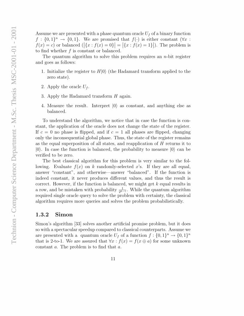
Assume we are presented with a phase quantum oracle Uf of a binary functionf : 0, 1n → 0, 1. We are promised that f(·) is either constant (∀x :f(x) = c) or balanced (
∣∣x : f(x) = 0∣∣ =
∣∣x : f(x) = 1∣∣). The problem is
to find whether f is constant or balanced.The quantum algorithm to solve this problem requires an n-bit register
and goes as follows:
1. Initialize the register to H|0〉 (the Hadamard transform applied to thezero state).
2. Apply the oracle Uf .
3. Apply the Hadamard transform H again.
4. Measure the result. Interpret |0〉 as constant, and anything else asbalanced.
To understand the algorithm, we notice that in case the function is con-stant, the application of the oracle does not change the state of the register.If c = 0 no phase is flipped, and if c = 1 all phases are flipped, changingonly the inconsequential global phase. Thus, the state of the register remainsas the equal superposition of all states, and reapplication of H returns it to|0〉. In case the function is balanced, the probability to measure |0〉 can beverified to be zero.
The best classical algorithm for this problem is very similar to the fol-lowing. Evaluate f(x) on k randomly-selected x’s. If they are all equal,answer “constant”, and otherwise—answer “balanced”. If the function isindeed constant, it never produces different values, and thus the result iscorrect. However, if the function is balanced, we might get k equal results ina row, and be mistaken with probability 1
2k−1 . While the quantum algorithmrequired single oracle query to solve the problem with certainty, the classicalalgorithm requires more queries and solves the problem probabilistically.
1.3.2 Simon
Simon’s algorithm [33] solves another artificial promise problem, but it doesso with a spectacular speedup compared to classical counterparts. Assume weare presented with a quantum oracle Uf of a function f : 0, 1n → 0, 1n
that is 2-to-1. We are assured that ∀x : f(x) = f(x ⊕ a) for some unknownconstant a. The problem is to find that a.
11
Tec
hnio
n -
Com
pute
r Sc
ienc
e D
epar
tmen
t - M
.Sc.
The
sis
MSC
-200
1-01
- 2
001

The quantum algorithm to solve this problem requires two n-bit registersand goes as follows:
1. (a) Initialize the input register to H|0〉, and the output register to |0〉.(b) Apply the oracle Uf to the combined register.
(c) Apply the Hadamard transform H to the input register.
(d) Measure the input register. The result mi satisfies a · mi = 0,where ‘·’ denotes the inner product mod 2.
2. Repeat these steps until acquiring n linearly independent mi’s. Ex-tracting a from them is a straightforward polynomial classical process(Gauss-Jordan elimination) which requires no oracle queries.
The average number of repetition (and oracle queries) required to findthe linearly independent set of mi’s is O(n). An m with m · a = 1 is nevermeasured because of a special feature of the Hadamard transform—when|x〉+|x⊕a〉 are transformed, their “odd” |m〉 elements cancel out. A classicalalgorithm requires O(2n/2) oracle queries on average. Hence, in the case ofthis problem, quantum computation is exponentially faster than classicalcomputation.
1.3.3 Shor
Shor’s algorithm [32] solves two problem (Factorization and Discrete Log-arithm) whose hardness is the core of the security of RSA [29] and Diffie-Hellman [13] cryptographic protocols, respectively. Shor showed that boththe Factorization and the Discrete Logarithm problems are reducible to find-ing the period of a function. In the case of factorization, finding the primefactors p, q of N is equivalent to finding the period of fN,a(x) = ax mod N .(This is true for most a ∈ 2, . . . N − 1.)
Further, Shor showed how a period can be found efficiently using a quan-tum computer. The key algorithm to perform this task is the QuantumFourier Transform
∑
x
f(x)|x〉 QFT→∑
y
(1√N
∑
x
e2πixy/Nf(x)
)|y〉.
When |y〉 is measured, the outcome is in the close vicinity of the period off(x) with high probability. Two other important aspects are answered by
12
Tec
hnio
n -
Com
pute
r Sc
ienc
e D
epar
tmen
t - M
.Sc.
The
sis
MSC
-200
1-01
- 2
001

Shor: how the initial distribution∑
x f(x)|x〉 can be created efficiently for thegiven fN,a(x), and how to perform QFT efficiently. The overall complexityof Shor’s algorithm is O(log3 N) (polynomial in the number of bits), while
the best known classical algorithm’s complexity is Θ(ec(log N)1/3(log log N)2/3
)(super-polynomial in the number of bits).
1.4 The Structure of this Thesis
In Chapter 2 of this work we describe Grover’s original search algorithm. Weanalyze it using the eigenstates of the Grover Iterate. We take great effortto prove the somewhat obvious classical lower bound, and provide one of theproofs of the optimality of Grover’s algorithm.
In Chapter 3 we survey the various generalizations of the algorithm. Weanalyze them in a uniform method, and state what is the ultimate general-ization. One of the results of our analysis of one of the generalizations wascited by [7], and we provide it in full details here.
Chapter 4 presents and analyzes a new generalization of the algorithm,where the quantum register is allowed to be initialized in an arbitrary mixedstate. We provide an expression for the probability to measure a markedstate as a function of time, and a measure for its effectiveness, including athreshold under which the algorithm is ineffective. We use our result to givea counter-example to one of the results of Bose et al. [8].
We conclude our work by explaining why it may be considered as a sup-port to the common belief that entanglement is essential for true quantumcomputation.
In Appendix A we provide our proof of the equivalence of regular quantumoracles and phase quantum oracle. The proof we present of the optimalityof the algorithm (and other proofs, too) makes use of this equivalence.
13
Tec
hnio
n -
Com
pute
r Sc
ienc
e D
epar
tmen
t - M
.Sc.
The
sis
MSC
-200
1-01
- 2
001
Chapter 2
Grover’s Algorithm
Assume a binary function f : 0, . . . , N − 1 → 0, 1 such that
f(x) =
1, if x = k0, if x 6= k
for some unknown k (which is selected uniformly in the range 0, ..., N −1). Assume further that we may use a classical oracle of f(x). The searchproblem is to find this unknown marked value k. Our task is quite difficult—the best option is to try out all values in a random order. The expectednumber of oracle queries required to find the marked value is N
2. However,
if we may use a quantum oracle, we can follow Grover’s algorithm [18] and
find the marked value after π√
N4
queries on average.
2.1 Classical Lower Bound
Let AN be a classical search algorithm of size N . Let E(AN) be the expectednumber of queries that AN uses to find the marked value k.
Without loss of generality we assume that all the queries that AN asksare different, as if two of the queries are identical, there exists an equivalentmore efficient algorithm B that remembers the first answer and skips thesecond invocation of the query. Therefore, any lower bound we prove on Bis true for AN , too.
By virtue of the fact that information about f(·) is accessible only throughoracle queries, AN can identify k only by querying f(k). There is only oneexception, once N − 1 failed queries are asked, the only untested value must
14
Tec
hnio
n -
Com
pute
r Sc
ienc
e D
epar
tmen
t - M
.Sc.
The
sis
MSC
-200
1-01
- 2
001

be k since we know there is one. Therefore, AN defines a series of N oraclequeries, that is independent of the identity of k. Since the marked value k isselected uniformly from 0, ..., N − 1, the index ik of the query f(k) in theseries of queries is also distributed uniformly. For 1 ≤ t ≤ N , P (ik = t) = 1
N.
AN finds k after ik queries, except for k such that ik = N , where only N − 1queries are required. Thus, for any algorithm (deterministic or randomized),the expected number of required queries is at least
E(AN) =N∑
k=1
P (ik)ik =N−1∑
ik=1
ikN
+N − 1
N=
N + 1
2− 1
N.
2.2 The Quantum Algorithm
We assume along this thesis that the size of the search field N = 2n is anintegral power of 2. A search problem with f ′ : 1, ..., N ′ → 0, 1 whereN ′ is not a power of 2, is easily reducible to a problem of size N = 2n. Allthat has to be done is to define N as the next power of 2 and to define
f(x) =
f ′(x), 0 ≤ x ≤ N ′ − 10, N ′ ≤ x ≤ N − 1
.
Since N < 2N ′, the expected number of queries π√
N4
< π√
2N ′
4is at worst
√2
times larger than the case of an integral power of 2.In order to perform the algorithm we assume the existence of a quantum
computer with a computation register of n qubits, and the existence of aquantum oracle for the function f . The algorithm is as follows:
1. Initialize the register to H |0〉. That is, reset all qubits to |0〉 and applythe Hadamard transform to each of them. This produces an equalsuperposition of all states in the computation basis 1√
N
∑i |i〉.
2. Repeat the following operation (named the Grover Iterate Q) T = π√
N4
times:
(a) Rotate the marked state by a phase of π radians (Iπf ). This is
done by a single application of the phase quantum oracle.
(b) Apply the Hadamard transform on the register.
15
Tec
hnio
n -
Com
pute
r Sc
ienc
e D
epar
tmen
t - M
.Sc.
The
sis
MSC
-200
1-01
- 2
001

(c) Rotate the |0〉 state by a phase of π radians (Iπ0 ).
(d) Apply the Hadamard transform again.
(e) Negate the total phase of the register (This step has no physicalmeaning, and only provides some aid for understanding).
3. Measure the resulting state.
2.3 Analysis
A thorough study of this algorithm appears in [19, 9]. The simplest analysisis done in vector notation. The algorithm is initialized with
|ψ0〉 = H|0〉 =1√N
∑
i
|i〉, (2.1)
and thenQ = −HIπ
0 HIπf
= −H (I − 2|0〉〈0|) H (I − 2|k〉〈k|)= − (I − 2H|0〉〈0|H) (I − 2|k〉〈k|)
(2.2)
is applied iteratively, where |k〉 is the marked state. Let us now define anorthonormal basis:
• |k〉 the marked state
• |l〉 = 1√N−1
∑i6=k |i〉 (equal superposition of the unmarked states).
• Extend these two with additional N − 2 orthonormal vectors.
It is easily verified that in this basis
Q =
1 − 2N
2√
N−1N
−2√
N−1N
1 − 2N
−1. . .
−1
(2.3)
which is clearly a rotation matrix in the (|k〉, |l〉) plane, with angle ω wherecos ω = 1 − 2
N, and a phase flip in the orthogonal subspace. For large N , ω
16
Tec
hnio
n -
Com
pute
r Sc
ienc
e D
epar
tmen
t - M
.Sc.
The
sis
MSC
-200
1-01
- 2
001

can be approximated as ω ≈ 2√N
. The initial state
|ψ0〉 =1√N|k〉 +
√N − 1√
N|l〉 (2.4)
lies on the rotated plane, with angle φ ≈ 1√N
off the |l〉 axis. Thus,
|ψt〉 = Qt|ψ0〉 = sin(ωt + φ)|k〉 + cos(ωt + φ)|l〉, (2.5)
and the probability to measure the marked state
P (t) = |〈k|ψt〉|2 = sin2(ωt + φ) =1
2− 1
2cos(2ωt + 2φ) (2.6)
reaches one when 2ωt+2φ = π, after T ≈ π√
N4
iterations. Notice that T , thenumber of iterations needed to measure the marked state with certainty, isunlikely to be an integer. In the limit of large N , this is of no interest, sincethe P (t) for the integer nearest to T is very close to 1. Yet the question of howto find the marked state with certainty [22, 25] is interesting to the physicistsand engineers who are building the first small-scale implementations of thealgorithm (and cf. Subsection 3.5.2).
2.3.1 Rotation about the Average
Along with the description of the algorithm as a rotation of a plane, there ex-ists another description according to which the Grover Iterate Q = −HIπ
0 HIπf
is broken into two operations: the oracle query Iπf , and the rotation about
the average operator −HIπ0 H. The latter operation is a rotation about the
average due to the following. For arbitrary |ψ〉 =∑N
i=0 ai|i〉 described in thecomputation basis, the amplitudes average is
a =1
N
∑ai =
1
N
N∑
i=0
〈i| ·N∑
i=0
ai|i〉 =1√N〈0|H|ψ〉. (2.7)
To rotate all amplitudes about this average means to map
ai → ai − 2(ai − a) = 2a − ai. (2.8)
In vector notation it looks like
〈i|ψ〉 → 2√N〈0|H|ψ〉 − 〈i|ψ〉. (2.9)
17
Tec
hnio
n -
Com
pute
r Sc
ienc
e D
epar
tmen
t - M
.Sc.
The
sis
MSC
-200
1-01
- 2
001

Notice that 1√N
= 〈i|H|0〉, and therefore the mapping is
〈i|ψ〉 → 2〈i|H|0〉〈0|H|ψ〉 − 〈i|ψ〉. (2.10)
Since this is true for every 〈i|, it follows that the rotation about the averageoperation is after all 2H|0〉〈0|H − I = −HIπ
0 H†.
2.3.2 Punctuated Execution
One of the implications of the sinusoidal behavior of P (t) is that when theP (t) is near its maximal value, it doesn’t improve much with every iteration1.Thus, we can improve the expected required number of queries if we are will-ing to cut short of the maximal probability and risk repeating the algorithmin case of failure. Consider executing the algorithm for t iterations. Theexpected number of queries required to measure a marked state is
T =t
P (t)=
t
sin2(ωt + φ).
In the limit N ≫ 1 we can find its minimum using derivative and numericalanalysis. The minimum is reached when 2ωt ≈ tan(ωt) which is when ωt ≈1.1656 and
topt ≈0.742π
4
√N.
At that point
T ≈ 0.8785π
4
√N, (2.11)
which means a slight improvement comparing to the full-length execution.
2.4 Algorithm Optimality
Recently before the quantum search algorithm has been devised, Bennett,Bernstein, Brassard, and Vazirani [5] implicitly proved that a lower boundto the number of oracle queries required for unordered quantum search isO(
√N). Thus, Grover’s algorithm was known to be asymptotically optimal
since its birth. This, of course, did not deter [9, 17, 35, 8, 4, 2] and others
1This was first noted by Boyer et al. in [9], and later discussed in great detail byGingrich et al. in [16].
18
Tec
hnio
n -
Com
pute
r Sc
ienc
e D
epar
tmen
t - M
.Sc.
The
sis
MSC
-200
1-01
- 2
001

from providing additional proofs. Some of the proofs vary only in the extentof their similarity to the first one [5], their simplicity, and their tightness.Other approach the question of finding a lower bound in a more general way.
In this section we shall restate Grover’s proof [17] which appears to bethe simplest. We (assisted by [27]) extend that proof slightly to includeprobabilistic search algorithms, as was first done by Boyer et al. in [9].
At first we describe the most general search algorithm A: It may con-tain settings of qubits, unitary operations, oracle queries, and measurements.Without loss of generality we may assume that A begins with initializationof a quantum register, continues with unitary evolution of that register (in-cluding oracle queries), and ends with a measurement. Thus, any searchalgorithm A includes initialization to some oracle-independent state |ψ(0)〉and unitary evolution of the form UT OUT−1...U1OU0, where O is an oraclequery and U0...UT are oracle-independent unitary operations. The algorithmconcludes with a measurement. For A to be useful it has to find the markedstate with a bounded probability by some p, no matter what is the identityof the marked state. For simplicity of the proof we assume p = 1
2.
Consider different executions Ai of A, each with a different marked statei. Let |ψi(t)〉 be the state of the quantum register after UtOi...U1OiU0 isapplied, when the marked state is i. Oi denotes an oracle query when themarked state is i. Let |ψnull(t)〉 be the state of the quantum register afterUt...U0 is applied—with all oracle queries replaced by calls to the null oracle.
Definition 1 The Euclidean distance between two states |φ〉 =∑
i αi|i〉 and
|ψ〉 =∑
i βi|i〉 is defined by ‖|φ〉 − |ψ〉‖2,
∑i |αi − βi|2.
Definition 2 The spread of an execution Ai after t oracle queries is ∆2i (t) ,∥∥|ψi(t)〉 − |ψnull(t)〉
∥∥2.
Definition 3 The spread of A after t oracle queries is ∆2(t) ,∑N−1
i=0 ∆2i (t).
We prove the following 3 lemmas about the spread:
Lemma 1 The initial spread is zero.
The proof is straightforward: before the first step, all executions are equalto the null execution, and
∆2(0) =∑
i
∥∥|ψi(0)〉 − |ψnull(0)〉∥∥2
= 0
19
Tec
hnio
n -
Com
pute
r Sc
ienc
e D
epar
tmen
t - M
.Sc.
The
sis
MSC
-200
1-01
- 2
001

Lemma 2 In order to meet the bounded probability of success, the spread
has to be Ω(N).
Proof We know that the algorithm is successful with probability higher than12. That is, for every execution, when the register is finally measured at time
T , the marked state is found with probability > 12:
|〈ψi|i〉|2 ≥1
2. (2.12)
(Throughout this proof we discuss only the last step and therefore drop the(T ) qualifier for clarity.) The global phase of the final state of each executionhas no physical meaning, and thus may be assumed to satisfy 〈ψi|i〉 = |〈ψi|i〉|.Therefore, we may state that
α2(T ) ,∑
i
‖|ψi〉 − |i〉‖2
=∑
i
2 − 2 Re〈ψi|i〉 =∑
i
2 − 2|〈ψi|i〉|
and from (2.12),
≤ 2N −√
2N = (2 −√
2)N. (2.13)
Using Lagrange multipliers we can show that for real ai’s and bi’s and underthe constraint of
∑i |ai|2 + |bi|2 = 1, the expression
∑
i
ai ≤√
N
reaches its maximum when ai = 1√N
and bi = 0. Therefore, for every state,
and specifically for |ψnull〉
β2(T ) ,∑
i
∥∥|ψnull〉 − |i〉∥∥2
= 2N − 2 Re∑
i
〈i|ψnull〉
≥ 2N − 2√
N = 2N(1 − 1√N
). (2.14)
20
Tec
hnio
n -
Com
pute
r Sc
ienc
e D
epar
tmen
t - M
.Sc.
The
sis
MSC
-200
1-01
- 2
001

Using Cauchy-Schwarz inequality (that states that Re〈x|y〉 ≤∥∥x
∥∥2 ∥∥y∥∥2
)and by definition,
∆2(T ) =∑
i
∥∥|ψi〉 − |ψnull〉∥∥2
=∑
i
∥∥|ψi〉 − |i〉 + |i〉 − |ψnull〉∥∥2
= α2 − 2 Re∑
i
〈ψi − i|ψnull − i〉 + β2
≥ α2 − 2∑
i
∥∥|ψi〉 − |i〉∥∥∥∥|ψnull − |i〉〉
∥∥ + β2,
and applying Cauchy-Schwarz inequality again we arrive at
≥ α2 − 2√
α2β2 + β2
= (β − α)2.
From (2.13) and (2.14) we obtain
α ≤√
N
√2 −
√2 <
√N,
β ≥√
2√
N
√1 − 1√
N
>2√3
√N (for N ≥ 9)
and conclude that
∆2(T ) = (β − α)2
> N(2√3− 1)2 = O(N).
Lemma 3 The spread grows not faster than o(t2).
Proof At first we notice that
∆2i (t) =
∥∥|ψi(t)〉 − |ψnull(t)〉∥∥2
=∥∥Ui [Oi|ψi(t − 1)〉 − |ψnull(t − 1)〉]
∥∥2
=∥∥Oi|ψi(t − 1)〉 − |ψnull(t − 1)〉
∥∥2
= 2 − 2 Re〈ψnull(t − 1)|Oi|ψi(t − 1)〉
21
Tec
hnio
n -
Com
pute
r Sc
ienc
e D
epar
tmen
t - M
.Sc.
The
sis
MSC
-200
1-01
- 2
001

since the Euclidean distance is invariant under unitary transformations. Thus,
∆2i (t) − ∆2
i (t − 1) = 2 Re[〈ψnull(t − 1)|ψ(t − 1)〉−〈ψnull(t − 1)|Oi|ψi(t − 1)〉]
= 2 Re∑
j〈ψnull(t − 1)|j〉[〈j|ψ(t − 1)〉−〈j|Oi|ψ(t − 1)〉].
(2.15)
Without loss of generality (Cf. Appendix A) we assume that Oi is a phaseoracle, that is,
〈j|Oi|ψ〉 =
〈j|ψ〉, if j 6= i−〈j|ψ〉, if j = i
, (2.16)
and therefore
∆2i (t) − ∆2
i (t − 1) = 4 Re〈ψnull(t − 1)|i〉〈i|ψi(t − 1)〉≤ 4|〈i|ψnull(t − 1)〉||〈i|ψi(t − 1)〉|.
After subtracting and adding 〈i|ψnull〉, and dropping the (t − 1) qualifier,this becomes
= 4|〈i|ψnull〉| |〈i|ψi〉 − 〈i|ψnull〉 + 〈i|ψnull〉|,which is (by the triangle inequality),
≤ 4|〈i|ψnull〉| [|〈i|ψi〉 − 〈i|ψnull〉| + |〈i|ψnull〉|]= 4|〈i|ψnull〉| |〈i|ψnull〉 − 〈i|ψi〉| + 4|〈i|ψnull〉|2.
Now notice that for any a, b and any positive λ, (λ|a|−|b|)2 ≥ 0 and therefore
4|a||b| ≤ 2λ|a|2 +2
λ|b|2. (2.17)
Summing over all i’s, and applying this inequality,
∆2(t) − ∆2(t − 1) =∑
i
∆2i (t) − ∆2
i (t − 1)
≤ 4∑
i
|〈i|ψnull〉|2 + 2λ∑
i
|〈i|ψnull〉|2
+2
λ
∑
i
|〈i|ψnull〉 − 〈i|ψi〉|2
and since |〈i|ψnull〉 − 〈i|ψi〉|2 < ∆2i (t − 1),
≤ 4 + 2λ +2
λ∆2(t − 1). (2.18)
22
Tec
hnio
n -
Com
pute
r Sc
ienc
e D
epar
tmen
t - M
.Sc.
The
sis
MSC
-200
1-01
- 2
001

Substituting for λ = ∆(t − 1), this becomes
∆2(t) − ∆2(t − 1) ≤ 4∆(t − 1) + 4,
which is equivalent to∆(t) ≤ ∆(t − 1) + 2.
Since ∆(0) = 0, this means that
∆2(t) ≤ 4t2.
Together, these lemmas infer that A requires Ω(√
N) queries in order tofulfill its task. The first proof following this structure appeared as one ofthe weaknesses of quantum computing in Bennett et al.’s paper [5], beforeGrover’s algorithm has been devised. Zalka’s proof [35] follows that struc-ture, too, and gives the exact number of queries required to obtain certainprobability p.
Bose, Rallan and Vedral [8] give a similar, yet different proof. Insteadof following the evolution of the spread of the algorithm, they follow theentropy of the quantum register (See Eq. 4.8). They prove three propertiesof the entropy:
1. The initial entropy is zero, since the initial state is known to be H|0〉.
2. At the end of the algorithm the entropy must be log N , since the finalstate is the marked state, and there are N different possible markedstates occurring with equal probability 1
N. (Bose et al. do not dis-
cuss probabilistic algorithms, where the final state does not have 1-to-1mapping with the marked state.)
3. The entropy can grow by no more than 3√N
log N with each oracle query.
And again, the conclusion is that Ω(√
N) queries are required.
23
Tec
hnio
n -
Com
pute
r Sc
ienc
e D
epar
tmen
t - M
.Sc.
The
sis
MSC
-200
1-01
- 2
001

Chapter 3
Generalizations
Grover’s original algorithm described in Section 2.2 is quite restrictive. Inorder to make it more useful, to study its resistance to noise and to learnwhere its power stems from, the algorithm was generalized by many people.In this chapter we survey all known generalizations, and find the most generalone.
3.1 Many Marked States
The simplest generalization of Grover’s algorithm is to consider a functionwhere the number of x’s satisfying f(x) = 1 is r > 1. Not surprisingly, Boyeret al. show in [9] that finding one of the r marked x’s is easier when r is large,and the difficult search problem is when r ≪ N . Grover’s original algorithmrequires almost no changes in order to solve the problem of multiple markedstates. The only element that changes is the required number of iterations—
with r > 1 it is T = π4
√Nr. The analysis of the algorithm is very similar, too,
yet we have to be more careful while selecting the convenient orthonormalbasis. The N -dimensional Hilbert space of the register states may be brokeninto two subspaces: K of r dimensions, spanned by the marked states, andL of N − r dimensions, spanned by the unmarked states. The first basiselement for K is
|k〉 ,1√r
∑
i∈M
|i〉, (3.1)
24
Tec
hnio
n -
Com
pute
r Sc
ienc
e D
epar
tmen
t - M
.Sc.
The
sis
MSC
-200
1-01
- 2
001

where M is the set of all marked states. The rest of the basis is any orthonor-mal extension denoted by |k1〉 . . . |kr−1〉. A basis for L is
|l〉 ,1√
N − r
∑
i/∈M
|i〉. (3.2)
and any orthonormal basis extending it, denoted by |l1〉 . . . |lN−r−1〉. Inthe ordered basis (|k〉, |l〉, |k1〉 . . . |kr−1〉, |l1〉 . . . |lN−r−1〉),
Q =
1 − 2rN
2
√r(N−r)
N
−2
√r(N−r)
N1 − 2r
Nr−1︷ ︸︸ ︷
1. . .
1 N−r−1︷ ︸︸ ︷−1
. . .
−1
(3.3)
Ignoring the partial phase flip, Q is a 2-dimensional rotation with angle ω,where cos ω = 1− 2r
N. The initial state lies with angle φ to the |l〉 axis, where
cos φ = 〈0|H|l〉 =
√N − r
N.
For r ≪ N , ω ≈ 2√
rN
and φ ≈√
rN
. Thus, the probability to measure amarked space is again
P (t) =1
2− 1
2cos(2ωt + 2φ). (3.4)
Notice that the best time to measure, T ≈ π4
√Nr
depends on r. This is why
Gilles Brassard compares quantum search to baking a souffle—if you don’tknow when it is ready, you cannot enjoy it.
3.2 Unknown Number of Marked States
Another interesting question addressed by [9] is what happens when r isunknown. Is it then impossible to bake the souffle? They found out that it is
25
Tec
hnio
n -
Com
pute
r Sc
ienc
e D
epar
tmen
t - M
.Sc.
The
sis
MSC
-200
1-01
- 2
001
possible, and with no asymptotic penalty—it requires only O(√
Nr) queries.
All that is needed to accomplish that, is to start with a single application ofthe Grover Iterate. If the marked state is not found, repeat the algorithmwith a number of iterations which is 6
5times the previous number. Stop when
the number of iteration has reached π4
√N .
We give here a proof for a weaker result: When r ≪ N , the expectednumber of queries to find a marked state is O(
√N). Choose t ∈R 1 . . .
√N
and run t iterations of Grover’s algorithm. Since P (t) behaves like a smoothcosine (3.4), the expected value of P (t) is
∫ √N
0P (t′)dt′√N
=1
2+
sin 2ω√
N
4ω√
N>
1
2− 1
4ω√
N=
1
2− 1
8√
r>
3
8>
1
3. (3.5)
Thus, no more than 3 choices of random t are required on average, and amarked state is found in O(
√N) queries.
3.3 Arbitrary Pure Initial State
If Grover’s search algorithm is used as a procedure by another algorithm, itmight be necessary to avoid its initialization step. Even if the initializationis performed, gate imperfection or external noise might cause the outcome todiffer from the exact H|0〉 state. Rather, it may well be some general purestate |ψ0〉, which is a superposition of marked states and unmarked states.The first to address this problem were Biham et al. in [6], yet here we takeanother path taken by [16], and similar to [10].
Let us represent |ψ0〉 in the orthonormal basis of Section 3.1 (which isindependent of the initial state)
|ψ0〉 = |k〉〈k|ψ0〉 + |l〉〈l|ψ0〉 +r−1∑
i=1
|ki〉〈ki|ψ0〉 +N−r−1∑
i=1
|li〉〈li|ψ0〉
= Akeiθk |k〉 + Ale
iθl |l〉 +√
rσk|ψ0k〉 +√
N − rσl|ψ0l〉 (3.6)
where Akeiθk and Ale
iθl are defined as the unique polar representation of〈k|ψ0〉 and 〈l|ψ0〉, respectively. σk, |ψ0k〉, σl and |ψ0l〉 are defined such that√
rσk|ψ0k〉 and√
N − rσl|ψ0l〉 are the unique representation of their respec-tive terms as norm and normalized state.
26
Tec
hnio
n -
Com
pute
r Sc
ienc
e D
epar
tmen
t - M
.Sc.
The
sis
MSC
-200
1-01
- 2
001

The Grover Iterate is, of course, independent of the initial state. Thus,Q keeps the form of a 2-dimensional rotation matrix (3.3). This means that(except for signs) only the projections of |ψ0〉 on |k〉 and |l〉 are affected byQ, and that the state of the quantum register as a function of time is
|ψ(t)〉 = Qt|ψ0〉=
√rσk|ψ0k〉 + (−1)t
√N − rσl|ψ0l〉 + Ake
iθkQt|k〉 + AleiθlQt|l〉
=√
rσk|ψ0k〉 + (−1)t√
N − rσl|ψ0l〉+
(Ake
iθk cos ωt + Aleiθl sin ωt
)|k〉
+(Ale
iθl cos ωt − Akeiθk sin ωt
)|l〉 (3.7)
Let PK be the operator of projection on the marked subspace. The probabilityto measure a marked state as a function of the number of Grover iterationst is the squared amplitude of PK|ψ(t)〉:
P (t) =∣∣∣PK|ψ(t)〉
∣∣∣2
= rσ2k〈ψ0k|ψ0k〉 +
A2k + A2
l
2− 1
2
∣∣A2ke
2iθk + A2l e
2iθl∣∣ cos(2ωt + 2φψ0
)
= 〈Pψ0〉 − ∆Pψ0
cos(2ωt + 2φψ0). (3.8)
where
tan 2φψ0=
2AkAl cos(θl − θk)
A2k − A2
l
,
〈Pψ0〉 = rσ2
k +A2
k + A2l
2,
and
∆Pψ0=
1
2
∣∣A2ke
2iθk + A2l e
2iθl∣∣ .
The subscripts ψ0 denote that the values depend on the initial state. ω isindependent of the initial state, and as explained in Section 3.1, may beapproximated by ω = 2
√rN
. The probability to measure the marked state
reaches its maximum after T = π−2φ2ω
iterations.Our results are in agreement with previous works. For example, by our
definition √rσk|ψ0k〉 = PK(|ψ0〉 − |k〉〈k|ψ0〉).
27
Tec
hnio
n -
Com
pute
r Sc
ienc
e D
epar
tmen
t - M
.Sc.
The
sis
MSC
-200
1-01
- 2
001
This means that
σ2k = σ2
k〈ψ0k|ψ0k〉 =1
r
∑
i∈M
|〈i|ψ0〉 − 〈i|k〉〈k|ψ0〉|2 =1
r
∑
i∈M
|〈i|ψ0〉 − k|2 (3.9)
is the variance of 〈i|ψ0〉’s. This is exactly the definition of σk in [6]. Anotherexample is the original case studied by Grover, for which we find
⟨PH|0〉
⟩=
∆PH|0〉 = 12
and φH|0〉 ≈ 0. The maximum probability (≈ 1) is reached after
T = π√
N4
iterations.
3.4 Amplitude Amplification
Lov Grover [20, 21] reported that his algorithm works well when the Hadamardtransform is replaced by almost any other unitary operation. Brassard,Høyer, Mosca and Tapp took a slightly different approach in [10], wherethey call this idea “Amplitude Amplification”. They consider a search prob-lem with r marked states, and assume a quantum algorithm A that, wheninitialized by |0〉, finds one of the marked states with probability
Wk ,∑
i∈M
|〈i|A|0〉|2
and fails with probability Wl , 1−Wk. They showed that Grover’s algorithmmay be used to amplify this amplitude if it is initialized with A|0〉, and theGrover Iterate is modified to Q = −AIπ
0 A†Iπf . After applying Q iteratively
π4√
Wktimes, a marked state is found with almost certainty. In this perspec-
tive, the Hadamard transform in the original algorithm is a “blind guess”O(N) algorithm. Gingrich et al. [16] combined this generalization with thearbitrary initial state. We follow their analysis, since it hardly differs fromthat of Section 3.3. We start by defining
|k〉 ,1√Wk
∑
i∈M
|i〉〈i|A|0〉, (3.10)
and
|l〉 ,1√Wl
∑
i/∈M
|i〉〈i|A|0〉. (3.11)
28
Tec
hnio
n -
Com
pute
r Sc
ienc
e D
epar
tmen
t - M
.Sc.
The
sis
MSC
-200
1-01
- 2
001

|ki〉r−1i=1 and |li〉N−r−1
i=1 are defined accordingly to complete an orthonormalbasis. In this basis Q continues to be a rotation matrix, but now with angleω ≈ 2
√Wk. Similarly to (3.6) we represent |ψ0〉 in this new basis
|ψ0〉 = |k〉〈k|ψ0〉 + |l〉〈l|ψ0〉 +r−1∑
i=1
|ki〉〈ki|ψ0〉 +N−r−1∑
i=1
|li〉〈li|ψ0〉
= Akeiθk |k〉 + Ale
iθl|l〉 +√
Wkσk|ψ0k〉 +√
Wlσl|ψ0l〉
and re-define Akeiθk , Ale
iθl , σk, |ψ0k〉, σl and |ψ0l〉 accordingly. Notice thatnow
σ2k =
1
Wk
∑
i∈M
|〈i|A|0〉|2∣∣∣∣∣〈i|ψ0〉〈i|A|0〉 −
1
Wk
∑
j∈M
〈0|A|j〉〈j|ψ0〉∣∣∣∣∣
2
is the weighted variance of 〈i|ψ0〉’s, as defined in [7, Eq. (3.48)].
P (t) still adheres to Eq. (3.8), only that now 〈Pψ0〉 = Wkσ
2k +
A2k+A2
l
2.
3.5 General Rotations
The original Grover Iterate −HI0H†If has been further generalized to −UIβ
s U †Iγf
by Biham et al. [7]. That is, they use some arbitrary transformation U in-stead of Hadamard (this is equivalent to A in Section 3.4), arbitrary “pivot”state |s〉 instead of |0〉, and arbitrary phase rotations (β and γ) instead ofphase inversion. Actually, replacing |0〉 with |s〉 is superfluous. Let
Xs0 = I − |0〉〈0| − |s〉〈s| + |0〉〈s| + |s〉〈0|
be the swap operation between |0〉 and |s〉. For any U and |s〉 there existssome V = UXs0 such that
V Iβ0 V † = V
(I − (1 − eiβ)|0〉〈0|)
)V †
= U(I − (1 − eiβ)Xs0|0〉〈0|X†
s0
)U †
= U(I − (1 − eiβ)|s〉〈s|
)U †
= UIβs U †.
Their analysis of the generalized algorithm has been done in the methodof recursion equations, which they also used in [6]. We show that the vec-tor notation analysis, which is used throughout this work, is applicable too.
29
Tec
hnio
n -
Com
pute
r Sc
ienc
e D
epar
tmen
t - M
.Sc.
The
sis
MSC
-200
1-01
- 2
001

When represented in the orthonormal basis of the previous section, the gen-eralized Grover Iterate is
Q =
(M) r−1︷ ︸︸ ︷−eiγ
. . .
−eiγ N−r−1︷ ︸︸ ︷−1
. . .
−1
. (3.12)
The topmost 2-dimensional component of Q (in the |k〉, |l〉 subspace) is
M =
((1 − eiβ)eiγWk − eiγ
√WkWl(1 − eiβ)√
WkWleiγ(1 − eiβ) (1 − eiβ)Wl − 1
)
=
a b
√Wk
Wl
c√
Wl
Wkd
.
(3.13)
Since the elements of M are potentially complex, it cannot be interpretedimmediately as a rotation matrix. In order to analyze Q, we first diagonalizeM with M = SDS†, and write (as in [7]),
D =
(λ+
λ−
)=
(eiω+
eiω−
),
where
ω± = π +β + γ
2± ω
and
cos ω = Wk cosβ + γ
2+ Wl cos
β − γ
2. (3.14)
The eigenvectors of M , and their conjugates, are
|Ψ+〉 =
√Wk
Wlb|k〉 + (λ+ − a)|l〉
√Wk
Wl|b|2 + |λ+ − a|2
,
30
Tec
hnio
n -
Com
pute
r Sc
ienc
e D
epar
tmen
t - M
.Sc.
The
sis
MSC
-200
1-01
- 2
001

|Ψ−〉 =
√Wk
Wlb|k〉 + (λ− − a)|l〉
√Wk
Wl|b|2 + |λ− − a|2
,
〈Ψ+| =
√Wk
Wlb∗〈k| + (λ∗
+ − a∗)〈l|√
Wk
Wl|b|2 + |λ+ − a|2
=
√Wk
Wl|b|2 + |λ+ − a|2
λ− − λ+
λ− − a
b√
Wk
Wl
〈k| − 〈l|
,
and
〈Ψ−| =
√Wk
Wlb∗〈k| + (λ∗
− − a∗)〈l|√
Wk
Wl|b|2 + |λ− − a|2
=
√Wk
Wl|b|2 + |λ− − a|2
λ− − λ+
−λ+ − a
b√
Wk
Wl
〈k| + 〈l|
.
Therefore,
Qt|ψ0〉 = eiω+t|Ψ+〉〈Ψ+|ψ0〉 + eiω−t|Ψ−〉〈Ψ−|ψ0〉+(−1)teiγt
√Wkσk|ψ0k〉 + (−1)t
√Wlσl|ψ0l〉 (3.15)
and its projection on the marked subspace is
PKQt|ψ0〉 = eiω+t|k〉〈k|Ψ+〉〈Ψ+|ψ0〉 + eiω−t|k〉〈k|Ψ−〉〈Ψ−|ψ0〉+ (−1)teiγt
√Wkσk|ψ0k〉.
The probability to measure a marked state, which is the squared amplitudeof this projection, is
P (t) =∣∣eiω+t〈k|Ψ+〉〈Ψ+|ψ0〉 + eiω−t〈k|Ψ−〉〈Ψ−|ψ0〉
∣∣2 + Wkσ2k
= |〈k|Ψ+〉〈Ψ+|ψ0〉|2 + |〈k|Ψ−〉〈Ψ−|ψ0〉|2 + Wkσ2k
+ Re ei2ωt〈k|Ψ+〉〈Ψ+|ψ0〉〈ψ0|Ψ−〉〈Ψ−|k〉= Wk(z
21 + z2
2 + σ2k) − 2Wkz1z2 cos(2ωt + 2φ), (3.16)
where z1, z2, φ1 and φ are real and satisfy
z1
√Wke
iφ1 = 〈k|Ψ+〉〈Ψ+|ψ0〉and
31
Tec
hnio
n -
Com
pute
r Sc
ienc
e D
epar
tmen
t - M
.Sc.
The
sis
MSC
-200
1-01
- 2
001

−z2
√Wke
i(φ1−2φ) = 〈k|Ψ−〉〈Ψ−|ψ0〉.
We conclude that
P (t) = 〈P 〉 − ∆P cos(2ωt + 2φ),
where 〈P 〉 = Wk(z21 + z2
2 + σ2k) and ∆P = 2Wkz1z2.
3.5.1 δ-sensitivity of ∆P
With some algebra we obtain that
z1 =
∣∣∣∣1
λ− − λ+
((λ− − a)
〈k|ψ0〉√Wk
− 〈l|ψ0〉√Wl
b
)∣∣∣∣
z2 =
∣∣∣∣1
λ− − λ+
((λ+ − a)
〈k|ψ0〉√Wk
− 〈l|ψ0〉√Wl
b
)∣∣∣∣ .
In order to discuss our result we define the difference between the two rotationangles
δ , γ − β.
The two extreme cases of δ = 0 and δ = O(1) were discussed by Biham etal. [7]. Here we discuss the intermediate case where 0 < δ ≪ 1. One of ourresults was cited in [7], and we would like to present the full details here.Assuming Wk ≪ 1 (otherwise the algorithm is not of much use), we canapproximate (3.14) by
cos ω ≈ Wk cos β(1 − δ2
2) − Wk
δ
2+ (1 − Wk)(1 − δ2
8)
ω ≈√
2Wk
(1 − cos β +
δ
2sin β
)+
δ2
4. (3.17)
By definition ω± = π + β + δ2± ω, and through approximation of (3.13),
a = −eiγ + O(Wk) ≈ ei(γ+π),
b = 1 − eiβ + O(Wk)
and
|b|2 ≈ 2 (1 − cos β) .
32
Tec
hnio
n -
Com
pute
r Sc
ienc
e D
epar
tmen
t - M
.Sc.
The
sis
MSC
-200
1-01
- 2
001

λ+
λ−
ω
ω
ω+ = π + β + δ2
+ ω
ω− = π + β + δ2− ω
a
π + γ
π + β
π + β + δ2
δ
Figure 3.1: The relation between β, γ, ω±, and δδ-ו ω± ,γ ,β בין היחס
The approximations
λ− − a ≈ −(
ω +δ
2
)eiβ,
λ+ − a ≈ −(
ω − δ
2
)eiβ,
and|λ− − λ+| ≈ 2ω
are affirmed looking at Figure 3.1. Finally we can deal with ∆P , using k andl as shorthand for 〈k|ψ0〉√
Wkand 〈l|ψ0〉√
Wl, respectively:
∆P = 2Wkz1z2
≈ Wk
2ω2
∣∣∣∣(
ω +δ
2
)eiβk + bl
∣∣∣∣∣∣∣∣(
ω − δ
2
)eiβk + bl
∣∣∣∣
=Wk
2ω2
∣∣∣∣∣(keiβω − bl
)2 −(δkeiβ
)2
4
∣∣∣∣∣
=Wk
2ω2
∣∣∣∣b2l2 − 2blkeiβω + k2e2iβ
(ω2 − δ2
4
)∣∣∣∣
33
Tec
hnio
n -
Com
pute
r Sc
ienc
e D
epar
tmen
t - M
.Sc.
The
sis
MSC
-200
1-01
- 2
001

0
5
10
15
0
0.2
0.4
0.6
0.8
10
0.1
0.2
0.3
0.4
0.5
∆ P
β : 0, ..., π δ : 0, ..., 15√
Wk
Figure 3.2: ∆P as a function of β and δ, with constant Wk
קבוע Wk כאשר ,δ-ו β של כפונקציה ∆P
≈ Wk
2ω2
∣∣b2l2 − 2blkeiβω + k2e2iβ2Wk(1 − cos β)∣∣
<Wk
2ω2
(|b|2(1 + |k|2Wk) + 2|b||k|ω
)
<Wk
2ω2
(4(1 + 1) + 4
ω√Wk
)
and since by (3.17) ω > δ2,
<16Wk
δ2+
8√
Wk
δ(3.18)
which means that if δ ≫√
Wk, the algorithm hardly changes the probability.Figure 3.2 illustrates this behavior of ∆P . The special case of (3.18) forr = 1, Wk = 1/N and |ψ0〉 = U |0〉, was already discussed in [24].
3.5.2 Finding a Marked State with Certainty
The probability to measure a marked state as a function of time is given by asmooth cosine form (3.16). However, the first experimental implementationsof Grover’s algorithm use a small number of qubits which means that ω =O(2−n/2) is not that small, and it is probable that the optimal time to measure
34
Tec
hnio
n -
Com
pute
r Sc
ienc
e D
epar
tmen
t - M
.Sc.
The
sis
MSC
-200
1-01
- 2
001
the register falls far between two iterations. An interesting outcome of thearbitrary rotation generalization, is that one can carefully set β and γ so thatthe optimal time is exactly an integer. Algebraically, we search for β, γ, |ψ0〉and an integer t such that
P (t) = Wk(z21 + z2
2 + σ2k) − 2Wkz1z2 cos(2ωt + 2φ) = 1.
We do not solve this equation here. Recently, Høyer [22] and Long et al. [25]published two special solutions of this equation.
3.6 The Ultimate Generalization
In this section we discuss the most general iterative quantum process Rt. Weshow that any such R is a generalized Grover Iterate, where there may bemultiple “pivot” states with different β for each of them. Since R may beany unitary operation, this is the ultimate generalization conceivable.
Let f define an arbitrary number of marked states, and let γ be an arbi-trary rotation angle. Since any unitary operation has a unitary diagonaliza-tion [34], there exist U , a set of states S and a corresponding set of angles β
such that RI−γf = UI
~βSU †, where I
~βS rotates the phase of each of the states
in S by a possibly different angle. Let us now define
Q , R = UI~βSU †Iγ
f
According to the previous section, we know how Rt operates on arbitraryinput if S include a single state. If only we knew to analyze Q when Sincludes several states and ~β includes different elements, we would know howto analyze any iterative quantum process.
However, the analysis of such ultra-generalized algorithm has proved to bedifficult. To understand why, we consider A and B, two unitary operationsover the vector space CN . Let |ai〉na
i=1 and |bj〉nbj=1 be the eigenvectors
of A and B, respectively, whose eigenvalues are not 1. We may extendthese two sets into a complete basis with |cm〉N−na−nb
m=1 , unless for somej |bj〉 ∈ span(|ai〉na
i=1), in which case we would need more |cm〉’s. Nowlet us examine the operation AB. Since AB|cm〉 = A|cm〉 = |cm〉, it hasN − na − nb eigenvectors which are easy to find and whose eigenvalue is 1.Its other na+nb eigenvectors are most likely to have different eigenvalues, andare usually much harder to find. Before we understood this elementary linear
35
Tec
hnio
n -
Com
pute
r Sc
ienc
e D
epar
tmen
t - M
.Sc.
The
sis
MSC
-200
1-01
- 2
001

05
1015
2025
3035
0
10
20
30
400
5
10
15
20
25
30
35
bnan
#λ≠1
c
Figure 3.3: The number of eigenvalues which are not 1 as a function of na
and nb
nb-ו na של כפונקציה 1 שאינם העצמיים הערכים מספר
algebra fact, we checked it with Matlab and provide a graph in Figure 3.3.
In the context of this section, A = UI~βSU †, na = |S|, B = Iγ
f and nb = r.When |S| = 1, the problem degenerates into the simple rotation with partialphase rotations seen in (3.15). However, in general it remains a complexmulti-dimensional motion.
36
Tec
hnio
n -
Com
pute
r Sc
ienc
e D
epar
tmen
t - M
.Sc.
The
sis
MSC
-200
1-01
- 2
001

Chapter 4
Initialization with a Mixed
State
In this chapter we study the case where the original Grover Iterate, as de-fined in Section 2.2, is applied to a quantum register that is initialized to anarbitrary mixed state. This work is the first rigorous discussion of this case.In addition, our study extends and corrects a result from [8], and provides asimple approximation to the entropy of a pseudo-pure state (4.9). Our gen-eralization can be easily combined with the generalizations from Chapter 3.
4.1 Arbitrary Mixed Initial State
A mixed state arises when one cannot describe the state of a quantum systemdeterministically, no matter what basis one chooses (Cf. Subsection 1.2.4).Such a state appears very often when a quantum system is entangled withits environment, while the environment cannot be accessed or manipulated.
Extending the argument of Section 3.3, the initial state of the quantumregister might not be pure, due to external noise, decoherence or previousmanipulations. Instead, the initial state may be some general mixed state E .Given the description of E as an ensemble, all we can say is that the registeris in the pure state |ψi〉 with probability pi (for all i’s).
When the Grover algorithm is applied to the register whose state is |ψi〉,the probability to measure the marked state is Pi(t). The probability for theregister to be in that state is pi. Thus, the total probability to measure the
37
Tec
hnio
n -
Com
pute
r Sc
ienc
e D
epar
tmen
t - M
.Sc.
The
sis
MSC
-200
1-01
- 2
001

φ3
~∆P3
P1 P2
φ2
φ1
~∆P2
φ
~∆P1
P3
P
~∆P
Figure 4.1: The differences Pi − 〈Pi〉 as projections of a rotating ~∆Pi
מסתובבים ~∆Pi של כהיטלים Pi − 〈Pi〉 ההפרשים
marked state is the weighted average
P (t) =∑
i
piPi(t)
=∑
i
pi (〈Pi〉 − ∆Pi cos (2ωt + 2φi)) . (4.1)
The functions
Pi(t) − 〈Pi〉 = −∆Pi cos (2ωt + 2φi)
share a sinusoidal form, differing in amplitude and phase, but not in fre-quency. They may be thought of as the projections of vectors rotating infrequency ω, as exemplified in Figure 4.1. Therefore, their weighted sum(the Center of Mass of the vectors in the figure) is a sinusoidal function withthe same frequency:
P (t) = 〈P 〉 − ∆P cos(2ωt + 2φ
)(4.2)
where
〈P 〉 =∑
i
pi〈Pi〉, (4.3)
38
Tec
hnio
n -
Com
pute
r Sc
ienc
e D
epar
tmen
t - M
.Sc.
The
sis
MSC
-200
1-01
- 2
001

∆P =
√√√√(
∑
i
pi∆Pi cos 2φi
)2
+
(∑
i
pi∆Pi sin 2φi
)2
(4.4)
and
tan 2φ =
∑i pi∆Pi sin (2φi)∑i pi∆Pi cos (2φi)
. (4.5)
The probability to measure the marked state reaches its maximum value
Pmax = 〈P 〉 + ∆P (4.6)
after T = π−2φ2ω
iterations.If the algorithm is repeated until success with T iterations each time, the
expected total time to measure a marked state is
TQ =π − 2φ
2ωPmax
=π − 2φ
4Pmax
√N
since the number of repetition until success is distributed geometrically withparameter Pmax. If this value is significantly smaller than the classical ex-pected time TC = N/2, then the quantum algorithm has an advantage. Quan-titatively, the quantum algorithm is faster by a factor of
TC
TQ
=NωPmax
π − 2φ=
2Pmax
√N
π − 2φ. (4.7)
Of course, the constant factors in this expression have no real meaning untilwe know the relative “clock speed” of quantum computers. Notice that thisdefinition of the quantum advantage counts only oracle queries and does nottake into account the cost of repeated initialization of the register. In caseswhere the initialization is costly, arefind measure should be used.
4.2 Examples
4.2.1 Pure Initial State
When the arbitrary mixed state is chosen to be pure, the summations aredegenerate and the results of [6] are regained. For example, if the initial
39
Tec
hnio
n -
Com
pute
r Sc
ienc
e D
epar
tmen
t - M
.Sc.
The
sis
MSC
-200
1-01
- 2
001
state is the original E = p = 1, H|0〉, the original Grover case is found. If
E = p = 1, |k〉 (where |k〉 is the marked state), then 〈P 〉 = ∆P = 12
and
φ = π2. An interesting known property of the Grover algorithm is that for all
states orthogonal to both |k〉 and H|0〉, 〈P 〉 = ∆P = 0.
4.2.2 Pseudo-Pure Initial State
Ensembles where a pure state |ψ〉 appears with probability ǫ + 1−ǫN
and anystate orthogonal to it appears with equal probability of 1−ǫ
Nare called pseudo-
pure mixed states. They are written more conveniently as
ρǫ-pure =1 − ǫ
NI + ǫ|ψ〉〈ψ|.
Notice that 0 ≤ ǫ ≤ 1 is a measure of the purity of ρ: when ǫ = 0 it is totallymixed, and when ǫ = 1 it is totally pure. It is easy to see that in the limit of
large N , 〈P 〉 = ǫ 〈Pψ〉, ∆P = ǫ∆Pψ and φ = φψ. For example, for
ρ 1log N
-pure =1
N
(1 − 1
log N
)I +
1
log NH|0〉〈0|H,
we obtain 〈P 〉 = ∆P = 12 log N
and φ = 0. Notice that although ρ is extremely
mixed, the quantum advantage is of factor 2√
Nπ log N
= O(√
N).
4.2.3 Initial State Where m of the Qubits Are Mixed
Let us study the case where the register is initialized to
ρm-mix =1
2m
2m−1∑
i=0
H|i〉〈i|H.
This state may occur if the m least significant qubits of the register are totallymixed before the first Hadamard transform is applied. Since all H |i〉 areorthogonal to H |0〉 (except for H |0〉 itself) and they are almost orthogonalto |k〉 (since |〈k|H|i〉|2 = 1
N), the evolution of ρm-mix is governed by p =
2−m, H |0〉 and we obtain 〈P 〉 = ∆P = 12m+1 and φ = 0. The quantum
advantage is of factor 2√
N2mπ
: large m would render the algorithm useless.
40
Tec
hnio
n -
Com
pute
r Sc
ienc
e D
epar
tmen
t - M
.Sc.
The
sis
MSC
-200
1-01
- 2
001

4.3 Algorithm Usefulness and Entropy
The von Neumann entropy of a mixed state ρ is defined as
S(ρ) = −trρ log ρ. (4.8)
Bose et al. [8] presented a new model for quantum computation and laidout a new proof for the optimality of the Grover algorithm (Cf. Section 2.4).However, one of their results was the following: if the Grover algorithm isinitiated with a mixed state ρ, such that
S(ρ) ≥ 1
2log N,
the algorithm would have no advantage compared to the classical case. Thisis in disagreement with our findings: Bose et al. have a mistake regarding theentropy of the classical search problem1. This mistake does not invalidatethe other results in their paper.
A counter-example to their claim is the state ρ 1log N
-pure as defined above.
The entropy of the pseudo-pure state ρǫ-pure is
S(ρǫ-pure) = S
(1 − ǫ
NIN + ǫ|0〉〈0|
)
= −N−1∑
1
1 − ǫ
Nlog
1 − ǫ
N
−1 + (N − 1)ǫ
Nlog
1 + (N − 1)ǫ
N
= −(N − 1)1 − ǫ
Nlog
1 − ǫ
N
−1 + (N − 1)ǫ
Nlog
1 + (N − 1)ǫ
N,
and for large N , where N/(N − 1) ≈ 1,
≈ −(1 − ǫ) log1 − ǫ
N−
(1
N+ ǫ
)log
(1
N+ ǫ
)
= (1 − ǫ) log N − (1 − ǫ) log(1 − ǫ) −(
1
N+ ǫ
)log
(1
N+ ǫ
)
= (1 − ǫ) log N − ℓ, (4.9)
1Just above their Equation (10), they say that classical search can change entropy bylog
√N in
√N steps. This is true for a search field of size
√N , but wrong for the question
in matter where the search field is of size N .
41
Tec
hnio
n -
Com
pute
r Sc
ienc
e D
epar
tmen
t - M
.Sc.
The
sis
MSC
-200
1-01
- 2
001

where ℓ = (1−ǫ) log(1−ǫ)+(
1N
+ ǫ)log
(1N
+ ǫ)∈ [0, 0.88) for any 0 ≤ ǫ ≤ 1
and any N ≥ 2. For ǫ = 1log N
, we obtain ℓ ≈ 0 and
S(ρ 1log N
-pure) ≈(
1 − 1
log N
)log N = log N − 1.
This entropy is almost maximal. However, as noted above, the Grover algo-rithm outperforms any classical algorithm, even when it is initialized withthis state.
Entropy is not a good measure for the usefulness of the Grover algo-rithm. For almost every value of entropy, there exist states that are appli-cable as initializers and states that are not. For example (for n = log N),S(ρ(n−1)-mix) = log N − 1 = S(ρ 1
log N-pure), but when initialized in ρ(n−1)-mix,
the Grover algorithm is as bad as guessing the marked state. Another exam-ple may be given using the pure states H |0〉 〈0|H and H |1〉 〈1|H. With thefirst, Grover arrives at the marked state with quadratic speed-up, while thesecond is practically unchanged by the algorithm.
It seems as if Bose et al. had in mind only mixed states of the type ofSubsection 4.2.3 (ρm-mix). For these states, Grover’s algorithm is faster when
2√
N
2mπ> 1
which means also
m <1
2log N + 1 − log π ≈ 1
2log N
which in turn is almost identical to [8, Eq. (10)].
42
Tec
hnio
n -
Com
pute
r Sc
ienc
e D
epar
tmen
t - M
.Sc.
The
sis
MSC
-200
1-01
- 2
001

Chapter 5
Summary and Conclusions
In this work we have given a brief introduction to Quantum Computation.We presented Grover’s quantum search algorithm, and presented a proof thatit is the optimal search algorithm—better than any other, be it classical orquantum. Later we surveyed the various generalizations of this algorithm,some of which generalize the operations of the algorithm, and some generalizeits initial state. We have analyzed each of the generalization using the methodof eigenvector analysis of the Grover Iterate. We stated what is the ultimategeneralization thinkable for the operations of the algorithm. Based on thework of Biham et al., we generalized the initial state of the algorithm further,so we can deal with arbitrary mixed initial states.
Particularly, we studied how the algorithm behaves when initialized witha pseudo-pure initial state. We have shown that Grover’s algorithm is betterthan any classical algorithm in some exponentially mixed state. Braunsteinet al. [11] showed that mixed-enough states are separable. Had we founda separable state with better-than-classical behavior, it would have had re-sounding implications: it would have implied that entanglement is not essen-tial for non-trivial quantum computation. However, a careful examinationof [11] shows that our results provides some evidence to the contrary.
Figure 5.1 is a cross-section of the Bloch sphere. Braunstein et al. showedthat when ǫ ≥ 1
1+√
N, inseparable states are appearing. Notice that according
to Subsection 4.2.2, the quantum advantage of Grover’s algorithm which isinitialized with the pseudo-pure state ρǫ-pure = 1−ǫ
N+ ǫH|0〉〈0|H is of factor
2ǫ√
N/π. From this we learn that a necessary condition for a quantumspeed-up is ǫ > π
2√
N. These two thresholds coincide up to a constant factor.
This result may be considered as an evidence (although not a proof) that
43
Tec
hnio
n -
Com
pute
r Sc
ienc
e D
epar
tmen
t - M
.Sc.
The
sis
MSC
-200
1-01
- 2
001

Totally mixed
separable
includes inseparables
pure states
may include inseparables
1
1+√
N 2
N2
log N√N
Figure 5.1: Braunstein et al.’s separability bounds on the Bloch ballבלוך כדור על ושותפיו בראונשטיין של הפריקות חסמי
inseparability is necessary for nontrivial quantum computation.Amazingly or not, we observe that a similar result appears when con-
sidering Simon’s algorithm (Cf. Section 1.3.2), which performs well onlywhen initialized with the pure state H|0〉. If it is initialized with the ρ =1−ǫN
+ ǫH|0〉〈0|H pseudo-pure state and repeated until success, the expected
number of queries needed is O( log Nǫ
). Since the best classical solution re-
quires O(√
N) queries, the quantum advantage is of factor ǫ√
Nlog N
. Again, this
implies that if ǫ < 11+
√N
, the quantum advantage vanishes.
44
Tec
hnio
n -
Com
pute
r Sc
ienc
e D
epar
tmen
t - M
.Sc.
The
sis
MSC
-200
1-01
- 2
001

Appendix A
Oracle Equivalence
The regular quantum oracle and the controlled phase quantum oracle of abinary function f(·) were described in Subsection 1.2.5 and illustrated infigures 1.2 and 1.3. In this appendix, we prove that these two oracle modelsare equivalent. Let us define them rigorously, by describing how each operateson every element of the computation basis. The regular quantum oracle isthe operation
Uf : |x, y〉 → |x, y ⊕ f(x)〉,and the controlled phase quantum oracle is
c-pUf : |x, c〉 → (−1)c·f(x)|x, c〉.
Figure A.1 demonstrates the reduction Uf ≥ c-pUf , where H denotes theHadamard transform of a single qubit. Inspired by [26, page 113], we addedthe control bit to the known construction of an uncontrolled phase oracleusing a regular oracle. Figure A.2 demonstrates the reduction c-pUf ≥ Uf .We apply the Hadamard transform to the control line of c-pUf before andafter the oracle query. Each transform cancels out its respective Hadamardtransform from the previous construction, and returns the oracle to its simpleform.
Initially we check the reduction Uf ≥ c-pUf for the two possible values ofc, and for arbitrary value of x:
|x, 0〉 H→ 1√2
(|x, 0〉 + |x, 1〉)
Uf→ 1√2
(|x, f(x)〉 + |x, 1 ⊕ f(x)〉)
45
Tec
hnio
n -
Com
pute
r Sc
ienc
e D
epar
tmen
t - M
.Sc.
The
sis
MSC
-200
1-01
- 2
001

Uf
|c〉 H - |c〉H-
- -|x〉 (−1)c·f(x)|x〉
Figure A.1: Construction of a controlled phase quantum oracle using a reg-ular quantum oracle
רגיל קוונטי אורקל באמצעות מותנה פאזה אורקל בניית
pUf
uH H- -|y〉 |y ⊕ f(x)〉
- -|x〉 |x〉
Figure A.2: Construction of a regular quantum oracle using a controlledphase quantum oracle
קוונטי פאזה אורקל באמצעות רגיל קוונטי אורקל בניית
46
Tec
hnio
n -
Com
pute
r Sc
ienc
e D
epar
tmen
t - M
.Sc.
The
sis
MSC
-200
1-01
- 2
001

=1√2
(|x, 0〉 + |x, 1〉)H→ |x, 0〉 = (−1)0·f(x)|x, 0〉,
and
|x, 1〉 H→ 1√2
(|x, 0〉 − |x, 1〉)
Uf→ 1√2
(|x, f(x)〉 − |x, 1 ⊕ f(x)〉)
=(−1)f(x)
√2
(|x, 0〉 − |x, 1〉)H→ (−1)1·f(x)|x, 1〉.
Similarly, the opposite reduction is checked for the two possible values of y,and for arbitrary |x〉:
|x, 0〉 H→ 1√2
(|x, 0〉 + |x, 1〉)
c-pUf→ 1√2
(|x, 0)〉 + (−1)f(x)|x, 1〉
)
H→ |x, 0 ⊕ f(x)〉,and
|x, 1〉 H→ 1√2
(|x, 0〉 − |x, 1〉)
c-pUf→ 1√2
(|x, 0〉 − (−1)f(x)|x, 1〉
)
H→ |x, 1 ⊕ f(x)〉.
47
Tec
hnio
n -
Com
pute
r Sc
ienc
e D
epar
tmen
t - M
.Sc.
The
sis
MSC
-200
1-01
- 2
001

Bibliography
[1] Dorit Aharonov, Alexei Kitaev, and Noam Nisan. Quantum cir-cuits with mixed states. In Proceedings of the 30th Annual ACM
Symposium on Theory of Computing, pages 20–30, 1998. Also inquant-ph/9806029.
[2] Andris Ambianis. Quantum lower bounds by quantum arguments.In Proceedings of the 32nd annual ACM Symposium on Theory
of computing, pages 636–643, 21–23 May 2000. Also in quant-ph/0002066.
[3] Adriano Barenco. A universal two-bit gate for quantum com-putation. Proc. R. Soc. London A, June 1995. Also in cond-mat/9505016.
[4] Robert Beals, Harry Buhrman, Richard Cleve, Michele Mosca, andRoland de Wolf. Quantum lower bounds by polynomials. In Pro-
ceedings of the 39th IEEE Conference on Foundations of Computer
Science, pages 352–361, 1998. Also in quant-ph/9802049.
[5] Charles H. Bennett, Ethan Bernstein, Gilles Brassard, and UmeshVazirani. Strengths and weaknesses of quantum computing. SIAM
Journal on Computing, 26(5):1510–1523, October 1997. Also inquant-ph/9701001, as manuscript since 1994.
[6] Eli Biham, Ofer Biham, David Biron, Markus Grassl, andDaniel A. Lidar. Generalized Grover search algorithm for arbitraryinitial amplitude distribution. Phys. Rev. A, 60(4):2742–2745, Oc-tober 1999. Also in quant-ph/9711070.
[7] Eli Biham, Ofer Biham, David Biron, Markus Grassl, Daniel A.Lidar, and Daniel Shapira. Analysis of generalized Grover’s quan-
48
Tec
hnio
n -
Com
pute
r Sc
ienc
e D
epar
tmen
t - M
.Sc.
The
sis
MSC
-200
1-01
- 2
001
tum search algorithms using recursion equations. Phys. Rev. A,63:012310, January 2001. Also in quant-ph/0010077.
[8] Sougato Bose, Luke Rallan, and Vlatko Vedral. Communicationcapacity of quantum information. Phys. Rev. Lett., 85(25):5448–5451, 18 December 2000. Also in quant-ph/0003072.
[9] Michel Boyer, Gilles Brassard, Peter Høyer, and Alain Tapp. Tightbounds on quantum searching. Fortsch. Phys., 46:493–506, 1998.Also in quant-ph/9605034.
[10] Gilles Brassard, Peter Høyer, Michele Mosca, and Alain Tapp.Quantum amplitude amplification and estimation. In quant-ph/0005055, 2000.
[11] Samuel L. Braunstein, Carlton M. Caves, Richard Jozsa, NoahLinden, Sandu Popescu, and Rudiger Schack. Separability of verynoisy mixed states and imlications for NMR quantum comput-ing. Phys. Rev. Lett., 83(5):1054, August 1999. Also in quant-ph/9811018.
[12] David Deutsch and Richard Jozsa. Rapid solution of problemsby quantum computation. Proceedings of the Royal Society of
London, Series A, A439:553–558, 1992.
[13] Whitfield Diffie and Martin E. Hellman. New directions in cryptog-raphy. IEEE Transactions on Information Theory, 22(6), Novem-ber 1976.
[14] David P. DiVincenzo. Two-bit gates are universal for quantumcomputation. Phys. Rev. A, 51(2):1015–1022, February 1995. Alsoin cond-mat/9407022.
[15] Edward Fredkin and Tommaso Toffoli. Conservative logic. Inter-
national Journal of Theoretical Physics, 21(3/4):219–253, 1982.
[16] Robert M. Gingrich, Colin P. Williams, and Nicolas J. Cerf.Generalized quantum search with parallelism. Phys. Rev. A,61(5):052313, 2000. Also in quant-ph/9904049.
49
Tec
hnio
n -
Com
pute
r Sc
ienc
e D
epar
tmen
t - M
.Sc.
The
sis
MSC
-200
1-01
- 2
001

[17] Lov K. Grover. How fast can a quantum computer search. Inquant-ph/9809029.
[18] Lov K. Grover. A fast quantum mechanical algorithm for databasesearch. In Proceedings of the Twenty-Eighth Annual ACM Sympo-
sium on Theory of Computing, pages 212–219, New York, 22–24May 1996. ACM Press.
[19] Lov K. Grover. Quantum mechanics helps in searching for a needlein a haystack. Phys. Rev. Lett., 79(2):325–328, July 1997. Also inquant-ph/9706033.
[20] Lov K. Grover. Quantum computers can search rapidly by usingalmost any transformation. Phys. Rev. Lett., 80(19):4329–4332,May 1998. Also in quant-ph/9712011.
[21] Lov K. Grover. Quantum search on structured problems. InQCQS: NASA International Conference on Quantum Comput-
ing and Quantum Communications, QCQS. LNCS, 1998. Alsoin quant-ph/9802035.
[22] Peter Høyer. Arbitrary phases in quantum amplitude amplifica-tion. Phys. Rev. A, 62:052304, 2000.
[23] Richard Jozsa. Searching in Grover’s algorithm. In quant-ph/9901021, January 1999.
[24] Gui Lu Long, Yan Sung Li, Wei Lin Zhang, and Chang CunTu. Dominant gate imperfection in Grover’s quantum search al-gorithm. Phys. Rev. A, 61(4):042305, April 2000.
[25] Gui Lu Long, Li Xiao, and Yang Sun. General phase matchingcondition for quantum searching. In quant-ph/0107013.
[26] Michele Mosca. Quantum Computers Algorithms. PhD thesis,Wolfson College, University of Oxford, 1999.
[27] Michael A. Nielsen and Isaac L. Chuang. Quantum Computation
and Quantum Information. Cambridge University Press, 2000.
50
Tec
hnio
n -
Com
pute
r Sc
ienc
e D
epar
tmen
t - M
.Sc.
The
sis
MSC
-200
1-01
- 2
001
[28] John Preskill. Lecture notes for Physics 229: Quantum in-formation and computation. http://www.theory.caltech.edu-/people/preskill/ph229/notes/book.ps, September 1998.
[29] Ronald L. Rivest, Adi Shamir, and Leonard M. Adleman. Amethod for obtaining digital signatures and public key cryptosys-tems. CACM, 21(2), February 1978.
[30] Peter W. Shor. Fault-tolerant quantum computation. In Pro-
ceedings, 37th Annual Symposium on Fundamentals of Computer
Science, pages 56–65, 1995.
[31] Peter W. Shor. Scheme for reducing decoherence in quantum com-puter memory. Phys. Rev. A, 52(4):R2493–R2496, October 1995.
[32] Peter W. Shor. Polynomial-time algorithms for prime factorizationand discrete logarithms on a quantum computer. SIAM Journal
on Computing, 26(5):1484–1509, 1997.
[33] Daniel R. Simon. On the power of quantum computation. SIAM
Journal on Computing, 26(5):1474–1483, 1997.
[34] Vladimir I. Smirnov. Linear Algebra and Group Theory, pages180–184. Dover Publications, Inc., New York, 1970.
[35] Christof Zalka. Grover’s quantum searching algorithm is optimal.Phys. Rev. A, 60(4):2746–2751, October 1999. Also in quant-ph/9711070.
51
Tec
hnio
n -
Com
pute
r Sc
ienc
e D
epar
tmen
t - M
.Sc.
The
sis
MSC
-200
1-01
- 2
001

52
Tec
hnio
n -
Com
pute
r Sc
ienc
e D
epar
tmen
t - M
.Sc.
The
sis
MSC
-200
1-01
- 2
001

גרובר של הקוונטי החיפוש אלגוריתם
מעורבים ומצבים
קניגסברג דן
Tec
hnio
n -
Com
pute
r Sc
ienc
e D
epar
tmen
t - M
.Sc.
The
sis
MSC
-200
1-01
- 2
001

Tec
hnio
n -
Com
pute
r Sc
ienc
e D
epar
tmen
t - M
.Sc.
The
sis
MSC
-200
1-01
- 2
001

גרובר של הקוונטי החיפוש אלגוריתםמעורבים ומצבים
מחקר על חיבור
תואר לקבלת הדרישות של חלקי מילוי לשם
המחשב במדעי למדעים מגיסטר
קניגסברג דן
לישראל טכנולוגי מכון – הטכניון לסנט הוגש
2001 אוקטובר חיפה ה'תשס"ב Tחשוןec
hnio
n -
Com
pute
r Sc
ienc
e D
epar
tmen
t - M
.Sc.
The
sis
MSC
-200
1-01
- 2
001

Tec
hnio
n -
Com
pute
r Sc
ienc
e D
epar
tmen
t - M
.Sc.
The
sis
MSC
-200
1-01
- 2
001
המחשב. למדעי בפקולטה ביהם אלי פרופ' בהנחיית נעשה המחקר
המחקר. לאורך המסורה הנחייתו על ביהם לאלי מודה אני
זיו, לגלעד, מועילים, למאמרים והפניות פוריות שיחות על מור לטל להודות אבקש
בענייני המקוונת התמיכה על ולנדב לצפריר הקפה, בהפסקות חברתם על וארי פיליפ יובל,
זו. תיזה של הראשונה התבנית על וליוליה במטלאב, עזרתו על לעומר יוניקס/לאטך/עברית,
לו. אודה לא ולכן האינטיליגנטיות, הערותיו את בכתובים להזכיר שלא במפורש ביקש עידו
לסבי הלום, עד שהביאוני להורי ועידודה, אהבתה על לאביטל שלוחה מיוחדת תודה
זו. עבודה באשמת רבים ביקורים על שוויתרה ולסבתי וחשבון, קריאה אותי שלימד
הנדיבה הכספית התמיכה על ולטכניון טייסון וברתה מונטי ע"ש לקרן מודה אני
בהשתלמותי.
Tec
hnio
n -
Com
pute
r Sc
ienc
e D
epar
tmen
t - M
.Sc.
The
sis
MSC
-200
1-01
- 2
001

Tec
hnio
n -
Com
pute
r Sc
ienc
e D
epar
tmen
t - M
.Sc.
The
sis
MSC
-200
1-01
- 2
001

ענינים תוכן
1 תקציר
3 מבוא 1
3 . . . . . . . . . . . . . . . . . . . . . . . על מבט - קוונטי חישוב 1.1
6 . . . . . . . . . . . . . . . . . קוונטי חישוב של בסיסיים מרכיבים 1.2
6 . . . . . . . . . . . . . . . . . . . . . . . . . . . . מצבים 1.2.1
7 . . . . . . . . . . . . . . . . . . . . . . . . . . . פעולות 1.2.2
8 . . . . . . . . . . . . . . . . . . . . . . . . . . . . מדידה 1.2.3
8 . . . . . . . . . . . . . . . . . . . . . . . מעורבים מצבים 1.2.4
9 . . . . . . . . . . . . . . . . . . וקוונטיים קלסיים אורקלים 1.2.5
10 . . . . . . . . . . . . . . . . . . . . מוכרים קוונטיים אלגוריתמים 1.3
10 . . . . . . . . . . . . . . . . . . . . . . . . . דויטש-ג'וזה 1.3.1
11 . . . . . . . . . . . . . . . . . . . . . . . . . . . . סיימון 1.3.2
12 . . . . . . . . . . . . . . . . . . . . . . . . . . . . . שור 1.3.3
13 . . . . . . . . . . . . . . . . . . . . . . . . . . . . . התיזה מבנה 1.4
14 גרובר אלגוריתם 2
14 . . . . . . . . . . . . . . . . . . . . . . . . . . . קלסי תחתון סף 2.1
15 . . . . . . . . . . . . . . . . . . . . . . . . . הקוונטי האלגוריתם 2.2
16 . . . . . . . . . . . . . . . . . . . . . . . . . . . . . . . . ניתוח 2.3
17 . . . . . . . . . . . . . . . . . . . . . הממוצע סביב סיבוב 2.3.1
18 . . . . . . . . . . . . . . . . . . . . . . . . מקוצר ביצוע 2.3.2
18 . . . . . . . . . . . . . . . . . . . . . . . האלגוריתם אופטימליות 2.4
24 הכללות 3
24 . . . . . . . . . . . . . . . . . . . . . . . . רבים מסומנים מצבים 3.1
25 . . . . . . . . . . . . . . . . . מסומנים מצבים של ידועה לא כמות 3.2
26 . . . . . . . . . . . . . . . . . . . . . . . . שרירותי התחלתי מצב 3.3
א
Tec
hnio
n -
Com
pute
r Sc
ienc
e D
epar
tmen
t - M
.Sc.
The
sis
MSC
-200
1-01
- 2
001

28 . . . . . . . . . . . . . . . . . . . . . . . . . אמפליטודה הגברת 3.4
29 . . . . . . . . . . . . . . . . . . . . . . . . . . . כלליים סיבובים 3.5
32 . . . . . . . . . . . . . . . . . . . . . . . δ-ל ∆P רגישות 3.5.1
34 . . . . . . . . . . . . . . . . . בוודאות מסומן מצב מציאת 3.5.2
35 . . . . . . . . . . . . . . . . . . . . . . . האולטימטיבית ההכללה 3.6
37 מעורב במצב אתחול 4
37 . . . . . . . . . . . . . . . . . . . . שרירותי מעורב התחלתי מצב 4.1
39 . . . . . . . . . . . . . . . . . . . . . . . . . . . . . . . דוגמאות 4.2
39 . . . . . . . . . . . . . . . . . . . . . טהור התחלתי מצב 4.2.1
40 . . . . . . . . . . . . . . . . . . פסידו-טהור התחלתי מצב 4.2.2
40 . . . . . . . . לחלוטין מעורבים מהביטים m בו התחלתי מצב 4.2.3
41 . . . . . . . . . . . . . . . . . . . . ואנטרופיה האלגוריתם יעילות 4.3
43 ומסקנות סיכום 5
45 אורקלים שקילות א
ה בעברית תקציר
ב
Tec
hnio
n -
Com
pute
r Sc
ienc
e D
epar
tmen
t - M
.Sc.
The
sis
MSC
-200
1-01
- 2
001

איורים רשימת
9 . . . . . . . . . . . . . . . . . . . . . . . . . . הפיך קלסי אורקל 1.1
9 . . . . . . . . . . . . . . . . . . . . . . . . . . רגיל קוונטי אורקל 1.2
10 . . . . . . . . . . . . . . . . . . . . . . מותנה קוונטי פאזה אורקל 1.3
33 . . . . . . . . . . . . . . . . . . . . . . . . δ-ו ω± ,γ ,β בין היחס 3.1
34 . . . . . . . . . . . . . . . קבוע Wk כאשר ,δ-ו β של כפונקציה ∆P 3.2
36 . . . . . . . . nb-ו na של כפונקציה 1 שאינם העצמיים הערכים מספר 3.3
38 . . . . . . . . . . מסתובבים ~∆Pi של כהיטלים Pi − 〈Pi〉 ההפרשים 4.1
44 . . . . . . . . . בלוך כדור על ושותפיו בראונשטיין של הפריקות חסמי 5.1
46 . . . . . . . . רגיל קוונטי אורקל באמצעות מותנה פאזה אורקל בניית 1.א
46 . . . . . . . . קוונטי פאזה אורקל באמצעות רגיל קוונטי אורקל בניית 2.א
ג
Tec
hnio
n -
Com
pute
r Sc
ienc
e D
epar
tmen
t - M
.Sc.
The
sis
MSC
-200
1-01
- 2
001

ד
Tec
hnio
n -
Com
pute
r Sc
ienc
e D
epar
tmen
t - M
.Sc.
The
sis
MSC
-200
1-01
- 2
001

תקציר
לחשב ניתן מה את למצוא מנסה אשר החישוביות, תורת של שדה היא קוונטית חישוביות
של השמונים שנות בראשית הפיסיקלי. העולם של הקוונטי באופי התחשבות תוך ביעילות,
קוונטיות מערכות של שסימולציה פיינמן ריצ'רד נוכח שני, תואר ללמוד התחלתי בה המאה
מתהליכים פולינומית רדוקציה שאין היה נראה קשה. מטלה היא קלסי מחשב באמצעות
תת-מערכות n-מ המורכבת מערכת של הקוונטי המצב חישובית. לפעולה קוונטיים
מטריצה בידי נקבעת והתפתחותו מימדים, 2n בן מרוכב וקטורי למרחב שייך דו-מצביות
בעלות הסתכם ההתפתחות, של סימולציה לערוך ניסיון כל .2n × 2n שגודלה אוניטרית
מערכות שיש כיוון המתקבלת. הדיוק מידת או הדרוש הזמן מבחינת אקספוננציאלית
שתורת ייתכן – חבויה הזדמנות בכך ראה פיינמן ביעילות, זו את זו המדמות קוונטיות
הקונבנציונלים. המחשבים בידי מנוצלת שאינה יכולת מעניקה הקוונטים
חישוביים מודלים מתוכננים בו המחשב, מדעי של תחום היא החישוביות תורת
R ,RE – לפתור יכול הוא אותה הבעיות קבוצת מוגדרת מודל כל עבור נבחן. וכוחם
לחישוב ניתן מה היא החישוביות בתורת חשובה שאלה דוגמאות. כמה הן NPNP-ו
חישובי למודל אב-טיפוס הממשי. בעולם ומקום זמן של למגבלות התייחסות תוך בפועל,
למודל נחשבה היא רב זמן פולינומי. בזמן הפועלת טורינג מכונת הוא ובן-ביצוע, יעיל
זאת מנסחת צ'רץ'-טורינג תיזת של החזקה הגרסה ממשי. חישוב עבור האולטימטיבי
טורינג מכונת על-ידי לחישוב ניתן יעיל, לחישוב הניתנת פונקציה ש"כל באומרה במפורש
אקראי קלט גם לקבל מותר למכונה על-פיו חישובי מודל הוצע יותר מאוחר פולינומי". בזמן
ביעילות נוספות בעיות לפתור כנראה, מאפשר, זה מודל מסויימת. בהסתברות ולטעות
ה
Tec
hnio
n -
Com
pute
r Sc
ienc
e D
epar
tmen
t - M
.Sc.
The
sis
MSC
-200
1-01
- 2
001
החישוביות). בתורת רבות לשאלות בדומה פתוחה, עודנה נכונה זו טענה האם (השאלה
המגבלות הן מה לשאול דויטש דייויד את הוביל אולטימטיבי חישובי מודל אחר החיפוש
בן-ביצוע מודל הגדיר הוא מכך, כתוצאה ממשי. חישובי בתהליך המובנות הפיסיקליות
מודלים מהן טבעיות תופעות מנצל אשר הקיימים, מהמודלים לכאורה יותר וחזק לכאורה
מכונת פותרת אותה הראשונה המטלה את דויטש הציג 1985 בשנת התעלמו. קודמים
הוא ג'וזה ריצ'רד עם יחד קלסית. טורינג מכונת לעומת צעדים בפחות קוונטית טורינג
אולם קלסי, מחשב על-פני יתרון יש קוונטי למחשב בהן בעיות לסדרת זו מטלה הרחיב
במיוחד. מעניינת או קשה אינה עצמה והבעיה תת-אקספוננציאלי הינו זה יתרון
לפתור יכול קוונטי מחשב אותן בעיות מצאו סיימון, ואחריהם ווזיראני, ברנשטיין
ביותר המפורסם ההישג אולם יכול. אינו הסתברותי) (אפילו קלסי מחשב בעוד ביעילות,
מספר מפרק אשר ,(Peter Shor) שור של האלגוריתם הוא הקוונטית החישוביות של
אלגוריתם הוא נוסף הישג פולינומי. בזמן בדיד לוגריתם ומחשב הראשוניים לגורמיו
בודד איבר למצוא מצליח זה אלגוריתם .(Lov Grover) גרובר של הבלתי-ממוין החיפוש
גודל של הריבועי השורש של גודל בסדר שהוא בזמן בלתי-ממוין, בסיס-נתונים בתוך
בסיס-הנתונים.
לבנותו ניתן האם השאלה היתה קוונטי מחשב של מימוש בפני משמעותי מכשול
מבחינה הן חשובה, שאלה זו בניין". "אבני של סופית לקבוצה השייכים פשוטים משערים
מבחינה הן פשוט) בסיסי אלמנט ללא תעשייתי ייצור על לחשוב ניתן (לא פרקטית
איננה פשוטים מרכיבים באמצעות כללי קוונטי שער של סימולציה אם (כי תיאורטית
3 בן אוניברסלי שער שסיפק דויטש שוב זה היה זול.) כמשאב אותו לראות ניתן לא יעילה,
כניסות 2 בן מסויים בשער להשתמש שדי דיוינצ'נזו הראה יותר מאוחר ויציאות. כניסות
סביר. בדיוק חישוב כל לדמות על-מנת בודד, ביט של פאזה סיבוב בצירוף
מערכות של המובנית שבירותן היא מציאותי, קוונטי חישוב בפני נוסף חמור מכשול
הינם ופרודות, אטומים גרעינים, אלקטרונים, פוטונים, כגון חלקיקים הקוונטי. בסדר-הגודל
הם רעידות. או אלקטרו-מגנטי שדה טמפרטורה, שינויי כגון חיצוניות להפרעות רגישים
ו
Tec
hnio
n -
Com
pute
r Sc
ienc
e D
epar
tmen
t - M
.Sc.
The
sis
MSC
-200
1-01
- 2
001

ניתן שלא היה נראה אקראי. באורח מצבם את ולשנות ספונטני באופן אנרגיה לפלוט נוטים
דומים קשיים עם מתמודדים קלסי בחישוב מבוקר. באופן בו ולטפל קוונטי מידע לשמור
משלים אמצעי בעייתים. ערכים רענון תוך המידע, של רציפה ושמירה מדידה באמצעות
קוונטי, למידע מתאים אינו לחלוטין הראשון האמצעי שגיאות. לתיקון בקודים שימוש הוא
קורס המקורי המצב מפניו: להימנע רוצים אנו אשר את בדיוק עושה המדידה שפעולת כיוון
אשר עד קוונטי, מידע עבור השני האמצעי את להרחיב ניתן אם היה ברור לא ונהרס.
הוא יותר מאוחר ראשון. קוונטי שגיאות תיקון קוד של קיומו את שור פיטר הדגים ב-1995
.(fault-tolerant) לשגיאות חסין באופן השגיאות תיקון תהליך את לבצע כיצד הסביר
שלו, הבסיסי המרכיב הוגדר עצמאי. כמושג קוונטי מידע של המחקר התפתח בינתיים
קל למשל, וקלסי. קוונטי מידע בין מעניינים קשרים ונתגלו קיוביט), (או הקוונטי הביט
קוונטי מידע עבור זאת לעשות ניתן שלא קובע אי-השכפול משפט בעוד קלסי, מידע לשכפל
מוגדר קוונטי מידע של ביט :(Holevo) חולבו חסם הוא אחרת יסודית מסקנה שרירותי.
בודדת. בינארית ספרה ע"י מודר קלסי ביט בעוד בלתי-תלויים, ממשיים מספרים שני ע"י
קוונטי. ביט באמצעות אחד קלסי מביט יותר בנאמנות לקודד ניתן לא אולם
להעביר דרך מצאו ויזנר וסטיבן בנט צ'רלס ב-1992 כאשר הפתעה, זו היתה לפיכך
superdense) על-צפוף קידוד הקרויה זו תוצאה אחד. קיוביט לתוך המקודדים ביטים 2
משאב מנצלת היא המועבר, לקיוביט שבנוסף מכיוון חולבו, את סותרת אינה (coding
ניתן לחלופין, מראש. חלקו המתקשרים ששני (entangled) סבוכים קיוביטים זוג נוסף:
בתהליך שרירותי, קיוביט להעביר על-מנת קלסיים ביטים ובשני כזה סבוך בזוג להשתמש
של מעבר ללא מתבצעת הטלפורטציה למדי, מדהים באורח קוונטית. טלפורטציה הקרוי
סוגי שלושת כיצד השאלה המתקשרים. בין מוחלף אינו למידע פרט דבר שום – חומר
סביכות). לכמת הצורך גם (כמו פתוחה עודנה לזה זה מתייחסים הללו המשאבים
המפתח צפני את לתקוף מיכולתו נובע שור של האלגוריתם שעורר הרב הפרקטי העניין
מפתח להחלפת הקוונטי הפרוטוקול היא זו לחולשה תרופה שבשימוש. העיקריים הציבורי
מרוחקים משתמשים לשני מאפשר הוא .BB84 המכונה ברסרד, וז'יל בנט צ'רלס של סודי
ז
Tec
hnio
n -
Com
pute
r Sc
ienc
e D
epar
tmen
t - M
.Sc.
The
sis
MSC
-200
1-01
- 2
001

של בטיחותו מקבילים, קלסיים לפרוטוקולים בניגוד בסודיות. פרטית הודעה לזה זה לשלוח
הקוונטי בעולם קיים שהוא בכך רק אלא התוקף של החישובי בכוחו מותנית איננה BB84
שלנו.
המרכיבים את מציגים אנו קוונטית. לחישוביות קצר במבוא זו תיזה פותחים אנו
להשתנות, יכול זה מצב כיצד קוונטית, מערכת של מצב מהו – זה מדעי שדה של הבסיסיים
המודל על-פי .(mixed states) מעורבים קוונטים מצבים מהם וכן אותו, למדוד ניתן כיצד
(קיוביטים, קוונטיות סיביות ממספר מורכבת לחישוב המשמשת קוונטית מערכת המקובל,
טהור מצב נתון, רגע בכל קוונטי. רגיסטר נקראת כאלה סיביות כמה של קבוצה .(qubits
N = 2n בן הילברט במרחב יחידה וקטור הוא קיוביטים, n בן רגיסטר של (pure state)
,(computation basis) החישוב" ''בסיס הנקרא פורש בסיס מוגדר זה במרחב מימדים.
של לינארית קומבינציה הוא הרגיסטר של מצב .|N − 1〉 עד ב-〈0| מסומנים ואיבריו
ע"י המוגדר מרוכב מקדם מתאים איבר לכל כאשר שלהם), (סופרפוזיציה הבסיס איברי
אוניטרית היא סגורה קוונטית מערכת של מצב של בזמן ההתפתחות ופאזה. אמפליטודה
ומשמרת-הסתברות. הפיכה, לינארית, היא כלומר ,(unitary)
המדידה תוצאת מצבו. על ללמוד על-מנת החישוב בבסיס הרגיסטר את למדוד ניתן
האמפליטודה ריבוע היא מסויים בסיס איבר למדוד וההסתברות הבסיס, מאברי אחד תהיה
ואחריה אוניטרית (פעולה ניסוי לתכנן ניתן טהור מצב כל עבור זאת, עם לו. המתאימה
עבור זאת לעשות ניתן לא לכך, בניגוד בו. נמצא הרגיסטר האם בוודאות יאשר אשר מדידה)
במידה אקראית תהיה ניסוי כל של תוצאתו – (mixed state) מעורב במצב הנמצא רגיסטר
שהיתה יותר גדולה ממערכת חלק הוא אם מעורב למצב להגיע יכול רגיסטר מסויימת.
לקראת עבר). לכל התפזרה (למשל, לבלתי-נגישה הפכה המערכת שאר אך טהור, במצב
קוונטי פאזה אורקל ומהו פונקציה של רגיל קוונטי אורקל מהו מסבירים אנו ,1 פרק סוף
לזה. זה שקולים שהם א') (בנספח ומוכיחים שלה,
שהוא ההוכחות אחת ואת גרובר, של החיפוש אלגוריתם את מציגים אנו 2 בפרק
פחות דורש גרובר (אלגוריתם קבוע כפלי מקדם כדי עד האופטימלי החיפוש אלגוריתם
ח
Tec
hnio
n -
Com
pute
r Sc
ienc
e D
epar
tmen
t - M
.Sc.
The
sis
MSC
-200
1-01
- 2
001

גרובר של המקורי האלגוריתם קלסי). או קוונטי אחר, אלגוריתם כל לעומת אורקל קריאות
ואילו ,f(k) = 1 מתקיים ,k אחד, (בלתי-ידוע) ערך עבור רק מספרים, N שמתוך מניח
האלגוריתם .f הפונקציה ע"י המסומן הערך נקרא k .f(x) = 0 מתקיים x 6= k כל עבור
עליה. נוסף מידע שום לנו ידוע ולא בלבד, הפונקציה של קוונטי אורקל לנו נתון כי מניח
למצב הרגיסטר של באתחולו ומתחיל ביטים, log N בן קוונטי רגיסטר על פועל האלגוריתם
האלגוריתם מכן, לאחר .(|N − 1〉 עד מ-〈0| המצבים כל של אחידה (סופרפוזיציה H|0〉היפוכי הדמרד, טרנספורם לאורקל, קריאה כוללת איטרציה כל איטרציות. O(
√N) מבצע
קוונטית פעולה הוא ,H הדמרד, (טרנספורם נוסף. הדמרד וטרנספורם |0〉 למצב פאזה
הרגיסטר של מדידה לבצע יש לבסוף, העבודה.) בגוף בקצרה המתוארת ביותר שימושית
גרובר אלגוריתם לפיכך, .k תהיה המדידה תוצאת מוחלטת כמעט ובוודאות הקוונטי,
ניתן לא קלסיים שבאמצעים בעוד אורקל, קריאות O(√
N) לאחר k את לזהות מאפשר
קריאות. O(N)-מ בפחות זאת לעשות
מההכללות חלק רבים. מחברים בידי הוכללו האלגוריתם של השונים הפרמטרים
הורחב האלגוריתם האלגוריתם. של ההתחלתי המצב את – וחלקן האיטרטור, את מכלילות
כאשר מתנהג הוא כיצד ונבדק מסומנים, ערכים כמה המגדירות בפונקציות גם שיטפל כך
חיפוש, היוריסטיקות להאצת בו להשתמש שניתן הוכח שרירותי. במצב מאותחל הוא
אנו שרירותית. בזוית פאזה בסיבובי מוחלפים הפאזה היפוכי כאשר התנהגותו ונחקרה
אנו מהן ואחת אחת כל עבור אחידה. בשיטה אותן ומנתחים ,3 בפרק אלה הכללות סוקרים
האלגוריתם, במהלך הקוונטי הרגיסטר של המצב משתנה כיצד מחשבים נוח, בסיס מגדירים
ההכללה מהי מצאנו איטרציה. בכל מסומן ערך למדוד ההסתברות עבור לביטוי ומגיעים
הפרק. בסוף בכך דנים ואנו גרובר, של האיטרטור של האולטימטיבית
רשאי הוא בה האלגוריתם, של ההתחלתי המצב של חדשה הכללה מציגים אנו 4 בפרק
מסויים מצב למדוד ההסתברות עבור ביטוי נותנים אנו שוב, שרירותי. באופן מעורב להיות
יש זו לפונקציה מעורב, ההתחלתי המצב כאשר גם האיטרציות. מספר של כפונקציה
אולם חלשה. די הקוסינוס של האפליטודה מאוד, מעורב המצב וכאשר קוסינוס, צורת
ט
Tec
hnio
n -
Com
pute
r Sc
ienc
e D
epar
tmen
t - M
.Sc.
The
sis
MSC
-200
1-01
- 2
001

האלגוריתם בהם מקרים יש במיוחד, מעורב ההתחלתי המצב כאשר אפילו כי מראים אנו
הפסידו-טהור המצב היא לכך דוגמה קלסי. אלגוריתם מכל יותר טוב – היטב מתפקד
האלגוריתם כאשר .ǫ = 1log N
כאשר ρǫ-pure = 1−ǫN
+ ǫH|0〉〈0|H (pseudo-pure state)
לאחר יימצא המסומן המצב להצלחה, עד ושוב שוב עליו וחוזרים זה, במצב מאותחל
בממוצע. אורקל קריאות O(√
Nlog N
)
מצב של (von Neumann entropy) נוימן פון לאנטרופיית קירוב מספקים אנו
הפסידו-טהור. המצב של העירוב מידת עם רציף באופן גדלה שהיא ומצאנו פסידו-טהור,
לגבי הקודמת תוצאתינו בצירוף זה, קירוב .S(ρǫ-pure) ≈ (1− ǫ) log N אחד, ביט כדי עד
Bose, Rallan) ושותפיו בוזה של תוצאה תואם אינו האלגוריתם, של המוצלח תפקודו
האלגוריתם שכאשר לטענתם פשוטה נגדית דוגמה הוא ρ 1log N
-pure המצב .(Vedral-ו
מחיפוש יותר טוב אינו האלגוריתם ,12log N מ- גדולה האנטרופיה שבו במצב מאותחל
טעותם. חלה היכן מסבירים אנו כן, כמו קלסי.
פסידו-טהור, במצב הואמאותחל כאשר גרובר אלגוריתם בוחניםאתהשימושיותשל אנו
O(ǫ√
N) פי מהיר הוא ρǫ-pureב- מאותחל האלגוריתם כאשר יעילותו. עבור מדד ומספקים
– למיותר הופך הקוונטי האלגוריתם שמתחתיו קייםסף זה, מדד על-פי קלסי. אלגוריתם מכל
(inseparability bound) אי-הפריקות לחסם חופף זה שסף גילינו .ǫ < o(
1√N
)כאשר
Braunstein, Carlton, Caves, Jozsa, Linden, Popescu) ושותפיו בראונשטיין של
שלא פסידו-טהורים מצבים קיימים ,ǫ > 11+
√N
כאשר שלהם, החסם על-פי .(Schack-ו
כזה קוונטי רגיסטר של מצבו בודדים. קיוביטים מצבי של טנזורית למכפלה לפרקם ניתן
לכך כעדות זו תוצאה לראות ניתן .(inseparable, entangled) סבוך או בלתי-פריק, נקרא
בלתי-טריוויאלי. קוונטי חישוב עבור הכרחית הינה (entanglement (אי-פריקות, שסביכות
י
Tec
hnio
n -
Com
pute
r Sc
ienc
e D
epar
tmen
t - M
.Sc.
The
sis
MSC
-200
1-01
- 2
001