Grouping Pursuit in regression

Xiaotong Shen

School of StatisticsUniversity of Minnesota

Email: xshen@stat.umn.edu

Joint with Hsin-Cheng Huang (Sinica, Taiwan)

Workshop in honor of John Hartigan: Innovation and Inventiv eness in

Statistics Workshop, May 15-17, Yale

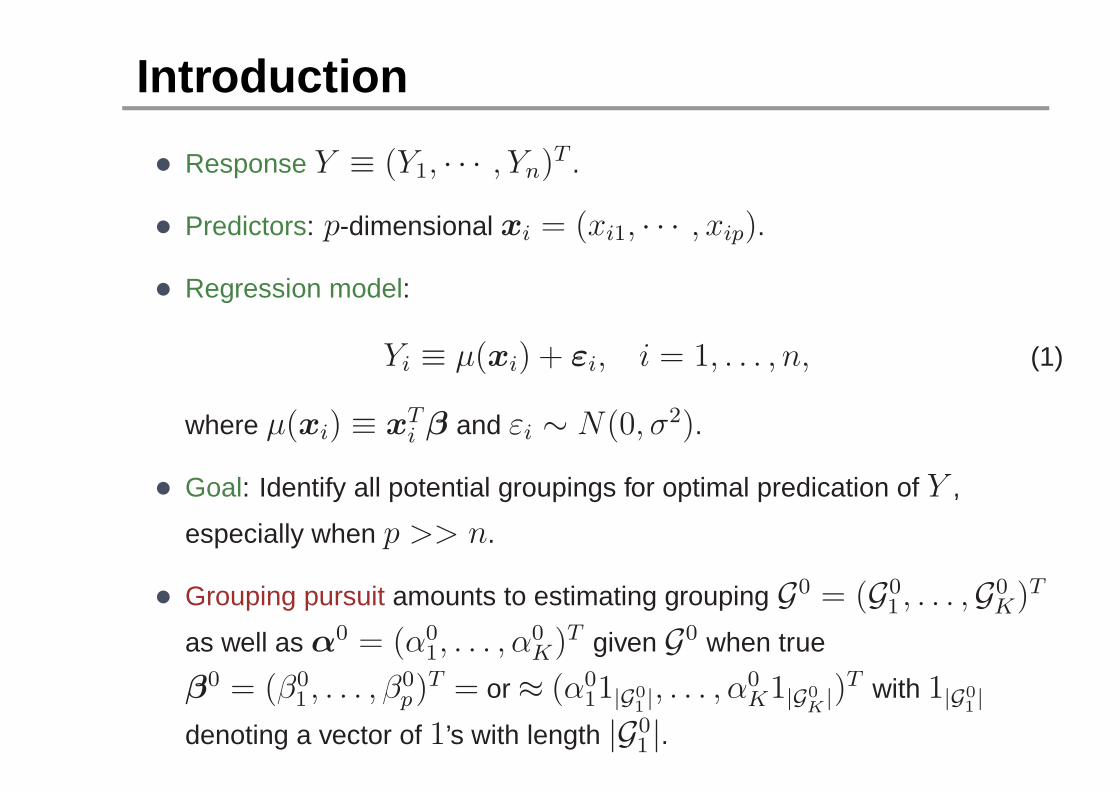
Introduction

• Response Y ≡ (Y1, · · · , Yn)T .

• Predictors: p-dimensional xi = (xi1, · · · , xip).

• Regression model:

Yi ≡ µ(xi) + εi, i = 1, . . . , n, (1)

where µ(xi) ≡ xTi β and εi ∼ N(0, σ2).

• Goal: Identify all potential groupings for optimal predication of Y ,

especially when p >> n.

• Grouping pursuit amounts to estimating grouping G0 = (G01 , . . . ,G

0K)T

as well as α0 = (α01, . . . , α

0K)T given G0 when true

β0 = (β01 , . . . , β

0p)

T = or ≈ (α011|G0

1 |, . . . , α0

K1|G0K|)

T with 1|G01 |

denoting a vector of 1’s with length |G01 |.

Grouping pursuit

• Essential to high-dimensional analysis is seeking a certain

low-dimensional structure.

◦ Homogenous subgroups. Variable selection seeks only two

homogenous groups: zero-coefficient group vs non-zero-coefficient

group.

◦ Projection pursuit, · · · .

• Main idea: Group coefficients of roughly the same value or size.

• Benefits: Variance reduction, which goes beyond variable selection.

Simpler model with higher predictive power. Can be thought of as one

kind of supervised clustering.

• Challenges: Complexity for identifying the best grouping is the pth order

Bell number: Bp = 1e

∑∞k=0

kp

k!–order eepa

for some 0 < a < 1.

Relevant literature and motivation

• Literature:

◦ Grouping in series order (F-Lasso, TSRZK, 05):∑p

j=1 |βj − βj+1|.

◦ Grouping in size (Bondell & Reich, 08):∑

i<j max(|βi|, |βj |).

◦ Grouping pursuit is one kind of supervised clustering,.....

• Motivating example:

Figure 1: Plot of the PPI gene subnetwork for breast cancer data

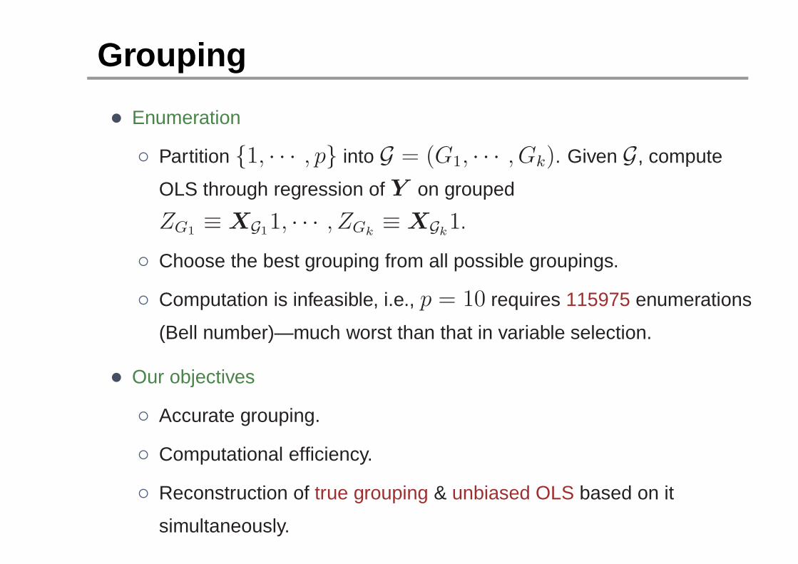
Grouping

• Enumeration

◦ Partition {1, · · · , p} into G = (G1, · · · , Gk). Given G, compute

OLS through regression of Y on grouped

ZG1 ≡ XG11, · · · , ZGk≡ XGk

1.

◦ Choose the best grouping from all possible groupings.

◦ Computation is infeasible, i.e., p = 10 requires 115975 enumerations

(Bell number)—much worst than that in variable selection.

• Our objectives

◦ Accurate grouping.

◦ Computational efficiency.

◦ Reconstruction of true grouping & unbiased OLS based on it

simultaneously.

Grouping pursuit–our approach

• Regularization through designed nonconvex penalty

S(β) =1

2n

n∑

i=1

(Yi − xTi β)2 + λ1J(β); J(β) =

∑

j<j′

G(βj − βj′),

(2)

where λ1 > 0 is a regularization parameter, G(z) = λ2 if |z| > λ2 and

G(z) = |z| otherwise, and λ2 > 0 is a thresholding parameter.

• Role of G(z)

◦ Piecewise linear for computational advantage through grouped

subdifferentials and difference convex (DC) programming.

◦ Three non-differentiable points: (a) z = 0 for grouping pursuit; (b)

z = ±λ2 for computation and for theoretical advantages.

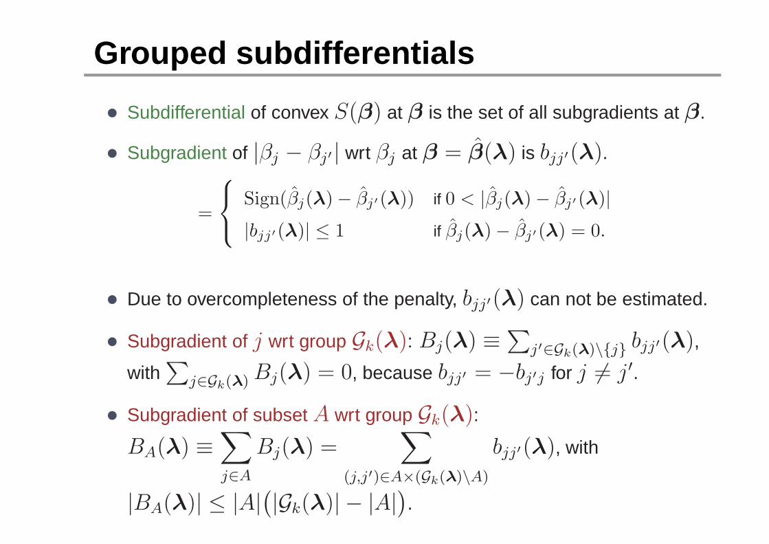
Grouped subdifferentials

• Subdifferential of convex S(β) at β is the set of all subgradients at β.

• Subgradient of |βj − βj′| wrt βj at β = β(λ) is bjj′(λ).

=

Sign(βj(λ) − βj′(λ)) if 0 < |βj(λ) − βj′(λ)|

|bjj′(λ)| ≤ 1 if βj(λ) − βj′(λ) = 0.

• Due to overcompleteness of the penalty, bjj′(λ) can not be estimated.

• Subgradient of j wrt group Gk(λ): Bj(λ) ≡∑

j′∈Gk(λ)\{j} bjj′(λ),

with∑

j∈Gk(λ) Bj(λ) = 0, because bjj′ = −bj′j for j 6= j ′.

• Subgradient of subset A wrt group Gk(λ):

BA(λ) ≡∑

j∈A

Bj(λ) =∑

(j,j′)∈A×(Gk(λ)\A)

bjj′(λ), with

|BA(λ)| ≤ |A|(|Gk(λ)| − |A|

).

Solution surface via DC programming

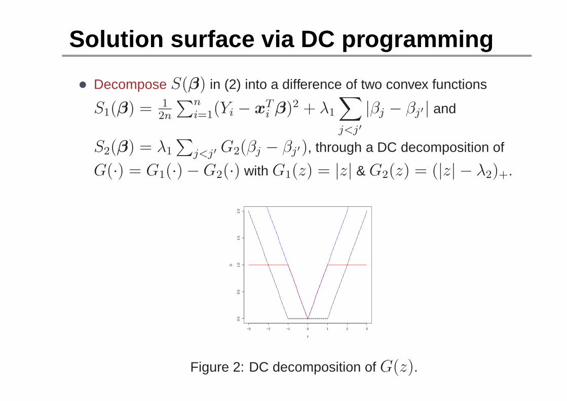
• Decompose S(β) in (2) into a difference of two convex functions

S1(β) = 12n

∑ni=1(Yi − xT

i β)2 + λ1

∑

j<j′

|βj − βj′| and

S2(β) = λ1

∑j<j′ G2(βj − βj′), through a DC decomposition of

G(·) = G1(·) − G2(·) with G1(z) = |z| & G2(z) = (|z| − λ2)+.

−3 −2 −1 0 1 2 3

0.0

0.5

1.0

1.5

2.0

z

G

;

;

;

;

;

;

;

;

;

;

;

;

;

;

;

;

;

;

;

;

;

;

;

;

;

;

;

;

;

;

;

;

;

;

;

;

;

;

;

;

;

;

;

:

:

:

:

:

:

:

:

:

:

:

:

:

:

:

:

:

:

:

:

: : : : : : : : : : : : : : : : : : : : :

:

:

:

:

:

:

:

:

:

:

:

:

:

:

:

:

:

:

:

:

Figure 2: DC decomposition of G(z).

Solution surface via DCP, continued

• Linearize S2(β) at iteration m by its affine minorization from iterationm − 1, leading to an upper convex approximating function at iteration m:

S(m)(β) = S1(β) − S2(β(m−1)(λ)) − (β − β(m−1)(λ))T∇S2(β

(m−1)(λ)), (3)

◦ ∇ : the subgradient operator; β(m−1)k (λ) : minimizer of (3) at

iteration m − 1.

• Solve (3) iteratively until it converges.

• No need to seek global solution—DC solution has desired optimality of a

global solution in grouping (Theorem), and can be computed much

efficiently (Theorem).

Homotopy method+DCP

• Key: homotopy via subdifferentials and DCP for solution β(m)(λ) of (3).

◦ Optimality through subdifferentials: ∇S(m)(β)|β=β(m)(λ) = 0.

• Major challenges: (1) (Discontinuity) β(m)(λ) may contain jumps in

(Y , λ2); (2) (Overcompleteness) computing B(m)j (λ) via enumerations

over {bjj′} is infeasible, (Bell number).

• Homotopy (1) piecewise linear and continuous in λ1 given (Y , λ2) with

piecewise linear penalty and designed support point. Transition

conditions: (1) Combining groups Gk(λ) with Gk(λ): αk(λ) = αl(λ);

(2) Splitting group Gk(λ): |BA(λ)| ≤ |A|(|Gk(λ)| − |A|

).

• Overcompleteness: Use piecewise linear property of B(m)j (λ) for

searching (order: O(p2 log p)).

• Homotopy Algorithm for computing β(λ) as a function of λ

simultaneously.

Homotopy method+DCP, continued

Property: terminate finitely and converge rapidly. Control at one λ0 implies

the entire surface.

**********

0 1 2 3 4

−0.

50.

00.

51.

01.

52.

02.

5

λ1

β

********** **********

**********

**********

**********

********** **********

**********

**********

**********

**********

**********

**********

**********

**********

********************

**********

**********

λ2 = 0.1

********************

0 1 2 3 4

−0.

50.

00.

51.

01.

52.

02.

5

λ1

β

******************** ******************** ********************

********************

**************************************** ******************** ****************************************

******************** ********************

********************

********************

********************

********************

******************** ********************

*

*******************

********************

λ2 = 0.5

1 2 3 4 5

12

34

5

λ1

λ 2

2.92.72.52.32.11.91.71.51.31.10.90.70.50.30.1−0.1−0.3−0.5−0.7−0.9

β1

1 2 3 4 5

12

34

5λ1

λ 2

2.92.72.52.32.11.91.71.51.31.10.90.70.50.30.1−0.1−0.3−0.5−0.7−0.9

β2

Figure 3: Regularization solution path/surface.

Model selection for prediction

• Model selection:

GDF(β(λ)) =1

2n

n∑

i=1

(Yi − µ(λ,xi)))2 +

1

nσ2df(λ), (4)

◦ For smooth β(λ) (m = 0), df(λ) = K(λ) for fast computation, c.f.,

SURE (Stein, 1981).

◦ For piecewise smooth β(λ) (m > 0),

df(λ) =σ2

τ 2

n∑

i=1

Cov∗(Yi, µ∗(λ,xi)) and Cov∗(Yi, µ

∗(λ,xi)),

through data perturbation (GSURE, Shen & Ye, 2002).

Theory: Error analysis

• Performance for grouping pursuit:

◦ Error: (Disagreement) P (G(λ) 6= G0) ≤ P (β(λ) 6= β(ols)).

G(λ),G0: estimated and true grouping (uniquely defined). β(λ), β(ols):

estimator defined by Algorithm 2 and OLS based on G0.

Theorem: P (β(λ) 6= β(ols)) is upper bounded by

K(K − 1)

2Φ

(−n1/2(γmin − λ2

)

2σc−1/2min

)+ pΦ

( −nλ1

σ max1≤j≤p ‖xj‖

). (5)

• Φ(z): CDF of N(0, 1).

‖xj‖: L2-norm of xj .

γmin: min{|α0k − α0

l | > 0 : 1 ≤ k < l ≤ K}.

cmin: smallest eigenvalue of ZTG0ZG0/n.

K : # of estimated groups, which is no larger than min(n, p).

Theory: Error analysis, continued

If max{ncmin(γmin − λ2)

2

8σ2,

nλ21

2σ2 max1≤j≤p

‖xj‖2/n

}− log p → ∞,

• Grouping Consistency

P (G(λ) 6= G0) ≤ P (β(λ) 6= β(ols)) → 0, p, n → +∞.

• Remarks:

◦ Roughly: p < exp(O(nλ21)), λ1 → 0, n1/2λ1 → ∞,

ncmin(γmin − λ2) → ∞. ( maxj:1≤j≤p

‖xj‖2/n bounded, satisfied by

standardization).

◦ Note that cmin can be independent of (p, n) or cmin → 0 as

p, n → ∞, depending on if K increases in (p, n), even though the

true model is independent of (p, n).

◦ A less sharp bound can be derived under a moment assumption of ε1.

Theory: Grouping

Let rj(β(λ)) = xTj

(Y − XT β(λ)

), which becomes the sample

correlation between xj and the residual, after standardization of

{xj : j = 1, . . . , p}.

Theorem: (Grouping) For any j = 1, . . . , p, j ∈ Gk(λ) if

|rj(β(λ)) − nλ1δk(λ)| ≤ nλ1(|Gk(λ)| − 1); k = 1, . . . ,K(λ). Here

δk(λ) = δ(m∗)(λ) and δ(m)(λ) is defined in Theorem 1.

• Predictors with similar values of correlations are grouped together, as

characterized by intervals ∪K(λ)k=1

(nλ1δk(λ) − nλ1(|Gk(λ)| −

1), nλ1δk(λ) + nλ1(|Gk(λ)| − 1))

.

Numerical examples

• Ex1: (Sparse grouping). In (2), εi ∼ N(0, σ2) and σ2 according to

SNR; xi ∼ N(0,Σp×p) with n = 50, p = 20 and

diagonal/off-diagonal elements 1/0.5;

β = (0, . . . , 0︸ ︷︷ ︸5

, 2, . . . , 2︸ ︷︷ ︸5

, 0, . . . , 0︸ ︷︷ ︸5

, 2, . . . , 2︸ ︷︷ ︸5

)T .

• Ex2: (Large p but small n). In(2), εi ∼ N(0, σ2), with SNR = 10;

xi ∼ N(0,Σ) with 0.5|j−k| the jk-th element of Σ. Here

β = (3, . . . , 3︸ ︷︷ ︸5

,−1.5, . . . ,−1.5︸ ︷︷ ︸5

, 1, . . . , 1︸ ︷︷ ︸5

, 2, . . . , 2︸ ︷︷ ︸5

, 0, . . . , 0︸ ︷︷ ︸180

)T .

• Mean squares error: averaged over 100 replications.

• Tuning: λ is estimated by minimizing GDF over grid points.

• Comparison: Convex (∑

j<j′ |βj − βj′|), OLS given estimated grouping.

Mean square error: Example 1

SNR=1 SNR=3 SNR=10

ConvexOLSDCPIdeal

n=50

MS

E

0.0

0.5

1.0

1.5

• DCP outperforms its convex counterpart and OLS based on estimated grouping.

• DCP is close to the ideal optimal performance when SNR is high.

• The average number of iterations is about 3-4.

Mean square error: Example 2

50,50 50,100 100,50 100,100

ConvexOLSDCPIdeal

p,n

MS

E

0.00

0.05

0.10

0.15

0.20

0.25

0.30

• DCP performs similarly as its convex counterpart and outperforms OLS based

on estimated grouping.

• DCP is not too close to the ideal optimal performance.

• The average number of iterations is about 2.

Take Away Messages

• Grouping in regression analysis can reduce estimation variance while

retaining the roughly the same amount of bias, leading to better predictive

accuracy.

• Develop its graph version.

• Study other types of grouping, e.g., grouping coefficients of similar size

not value, which involves the absolute values.