NASA Technical Memorandum 107626

// !" " . t/

;j2 :[

GROUND VIBRATION TESTS OF A HIGHFIDELITY TRUSS FOR VERIFICATION OF ONORBIT DAMAGE LOCATION TECHNIQUES

Thomas A. L. Kashangaki

May 1992

[q/ ANational Aeronautics and

Space Administration

Langley Research CenterHampton, Virginia 23665

(NASA-T_-I07626) GR_]UND VI_:RATIQN TESTS _F

A HIGH FIDELITY TRUSS FFJ_ VERIFICATION DF ON

f3RBIT C_AMAGE L_3CATION TECHNIQUES (NASA)

39 p_3/39

NgZ-Z7375

Uncl as

0 0 9 6 I2 9

https://ntrs.nasa.gov/search.jsp?R=19920018132 2020-04-04T03:17:48+00:00Z

g

ABSTRACT

This paper describes a series of modal tests that were performed on a cantilevered truss

structure. The goal of the tests was to assemble a large database of high quality modal

test data for use in verification of proposed methods for on orbit model verification and

damage detection in flexible truss structures. A description of the hardware is provided

along with details of the experimental setup and procedures for sixteen damage cases.

Results from selected cases are presented and discussed. Differences between ground

vibration testing and on orbit modal testing are also described.

INTRODUCTION

Future structures in space will be orders of magnitude larger and more complex than their

predecessors. Structures such as the Space Station Freedom will typically be built around

a large flexible frame and consist of truss members, habitat and experimental modules,

flexible and articulating appendages, along with numerous utility trays and moving parts.

The complexity and size of these structures, along with the need to design the spacecraft

to be lightweight, strong and modular for ease of expansion, repair and modification, all

require that the integrity of the structures be monitored periodically.

Several researchers [References 1, 2, 3 and 4] have proposed methods of detecting

damage to large space trusses and locating the site of this damage based on changes in the

vibration frequencies and modes of the structure. A research program underway at the

NASA Langley Research Center is using a hybrid-scale model of the Space Station as a

test-bed for studying the dynamic behavior of such structures. As part of this program,

researchers are studying the implementation of an on-orbit damage location scheme.

Results to date indicate that it may be possible to use the reaction control systems of the

space station to perform an on-orbit modal test of the structure and extract frequency and

mode shape data which might be used in this damage location technique.

In the past, damage location research has focused primarily on algorithm development

and verification using analytical models and simulated test data. Although often geared

towards large flexible space structures such as Space Station Freedom, researchers have

used simple structures to demonstrate and validate new "algorithms and techniques. The

most common verification models have been multiple spring-mass models. In order to

demonstratetherobustnessof their algorithms, researchers have attempted to simulate

measured modes and frequencies by adding a random error to the analytical mode

shapes. Very few researchers have reported using experimentally measured modal data

in their model updating and damage location methods. Smith and McGowan [5] were

the first to report comprehensive tests conducted specifically with damage location in

mind. The tests they performed were on a "generic" truss structure using off the shelf

hardware. Because of the low fidelity in the strut manufacturing, the tests were only

partially successful. Other researchers have reported successful modification of finite

element models based on experimentally acquired data, but to date no comprehensive

tests have been performed specifically for studying damage location.

In order to fill this significant gap and provide researchers with a reliable and

comprehensive database of measured data, a damage location test bed has been developed

at the NASA Langley Research Center. In this paper the focus structure will be

discussed, and the design and implementation of the test program will be described.i

EIGHT BAY TRUSS TEST BED.

Dynamic Scale Model Technology Program

The Dynamic Scale Model Technology (DSMT) research program at the NASA Langley

Research Center has the objective of developing scale model technology for verifying

the dynamic analysis methods for predicting the on-orbit response of large space

structures. To meet these goals DSMT has developed a hybrid scaled model of the

proposed Space Station Freedom (SSF). Hybrid scaling refers to the scaling method,

where the inertial properties of the components (the masses, and mass moments of

inertia) have been scaled down to 1/5th the full scale model, while the overall dimensions

have been scaled down to 1/10th full scale. This mixture of scaling results in a model

that has five times the frequencies, and is small enough to fit in a reasonably sized

laboratory. Several launch configurations of the proposed Space Station will be studied

to understand the global dynamics of each of the configurations, as well as to explore the

modeling requirements and the ability to predict the behavior of the fully assembled

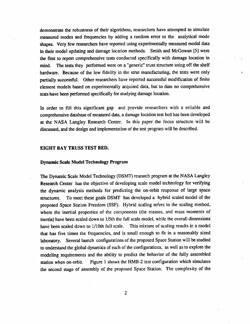
station when on-orbit. Figure 1 shows the HMB-2 test configuration which simulates

the second stage of assembly of the proposed Space Station. The complexity of the

2

ORIGINAL PAGE

BLACK AND WHITE PHOTOGRAPH

structure is evidenced by several large appendages such as solar arrays and radiators, and

the rigid pallets attached to the truss.

Figure 1 HMB-2 structure

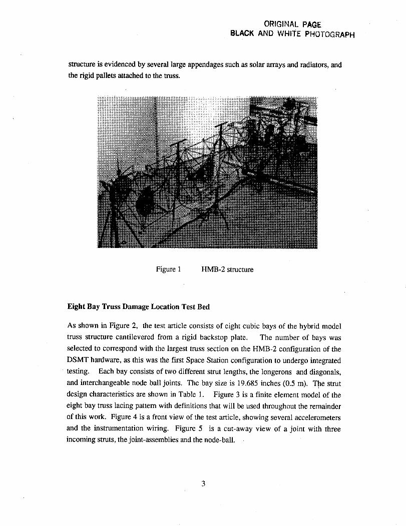
Eight Bay Truss Damage Location Test Bed

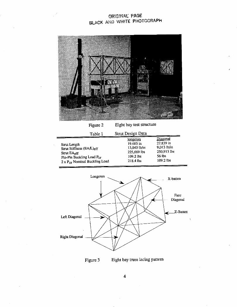
As shown in Figure 2, the test article consists of eight cubic bays of the hybrid model

truss structure cantilevered from a rigid backstop plate. The number of bays was

selected to correspond with the largest truss section on the HMB-2 configuration of the

DSMT hardware, as this was the first Space Station configuration to undergo integrated

testing. Each bay consists of two different strut lengths, the longerons and diagonals,

and interchangeable node ball joints. The bay size is 19.685 inches (0.5 m). T_ae strut

design characteristics are shown in Table 1. Figure 3 is a finite element model of the

eight bay truss lacing pattern with definitions that will be used throughout the remainder

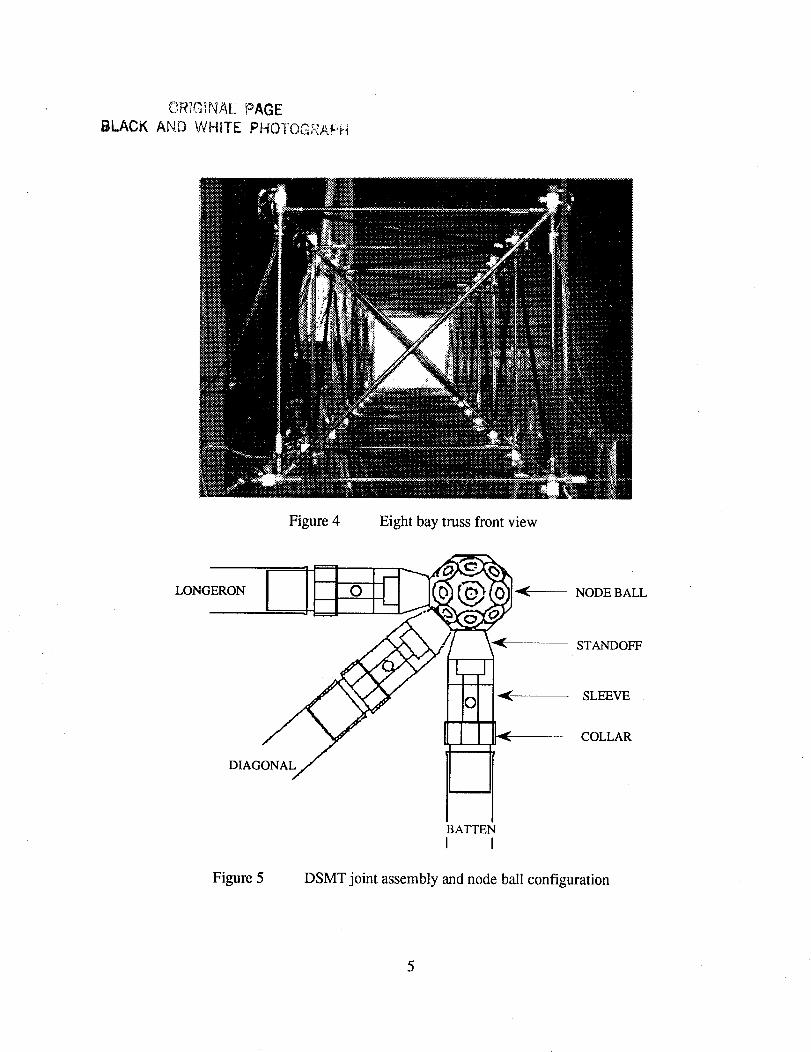
of this work. Figure 4 is a front view of the test article, showing several accelerometers

and the instrumentation wiring. Figure 5 is a cut-away view of a joint with three

incoming struts, the joint-assemblies and the node-ball.

ORIG!NAE PAGE

BLACK AND WHITE PHOTOGRAPH

Figure 2 Eight bay test structure

Table 1 Strut Design Data

Strut Length 19.685 in 27.839 inStrut Stiffness (EA/L)eff 13,040 lb/in 9,013 lb/in

Strut EAeff 225,669 lbs 250,913 lbsPin-Pin Buckling Load Pcr 109.2 lbs 56 lbs

2 x Pcr Nominal Buckling Load 218.4 lbs 109.2 lbs

Left Diagonal

Right Diagonal

Longeron _ _ J X-batten

_ _ DF_eal n

-Batte

Figure 3 Eight bay truss lacing pattern

4

ORIGTNAI.: PAGE

BLACK AND WHITE PHO1OC.,f:tAF, H

Figure 4 Eight bay truss front view

LONGERON O

DIAGONAL/

J

" " i

_2

NODE BALL

STANDOFF

SLEEVE

COLLAR

BATTEN

I I

Figure 5 DSMT joint assembly and node ball configuration

5

MODAL ANALYSIS AND TESTING.

Introduction

This section covers the basic theory of modal analysis and modal testing. It has been

summarized from a number of sources and has been included here for completeness.

There are two approaches to obtaining and studying the modai response of a structure.

The f'n'st of these is from mathematicai models of the structure, and the second is from

experimental modal analysis. Both of these approaches will be discussed here briefly.,

prior to a description of the tests that were performed.

In the first approach to modal analysis, mathematical models discretize a structure by

breaking it into numerous springs and masses which lend themselves well to simple

analysis. This process is typically performed by a finite element processor such as

MSC/NASTRAN TM [6] and SDRC I-DEAS TM [7]. The eigenvalue equation is then

solved using the multiple spring-mass representation and the normal modes and

frequencies of the complicated system are obtained. These modes can then be used in a

forced response analysis to examine the response of the system to a variety of inputs.

One very important forced response analysis is to input a unit force of varying frequency

at one node, while monitoring the response as a function of frequency at several

important locations. This response per unit force versus frequency is called the

Frequency Response Function (FRF) or transfer function.

Experimental modal analysis, on the other hand, starts out with the unit forced response

data (i.e. the FRFs) and extracts the modes of vibration directly from the FRFs without

having to make any assumptions about the mass and stiffness distribution. The

experimental modal analysis ends with a set of modes defined by frequency, damping,

mode shape coefficient and residue. Certain assumptions and post-processing of the data

are necessary to calculate modal mass and stiffness, with even further assumptions and

post-processing necessary to obtain physical stiffness or mass representations.

6

Modal Analysis Theory

Normal Modes Analysis

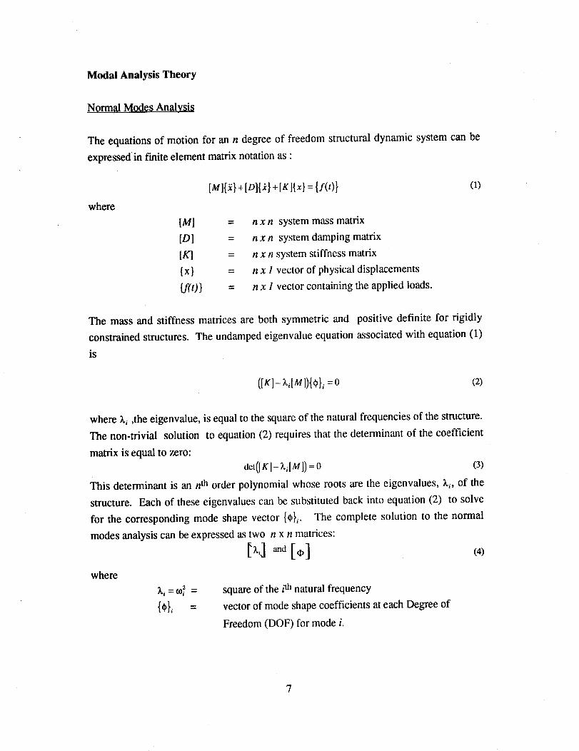
The equations of motion for an n degree of freedom structural dynamic system can be

expressed in finite element matrix notation as :

where

+ +[rl{x}={I(O}

[M] =

[D] =

IK! =

{x} =

If(t)} =

n x n system mass matrix

n x n system damping matrix

n x n system stiffness matrix

n x I vector of physical displacements

n x 1 vector containing the applied loads.

(1)

The mass and stiffness matrices are both symmetric and positive definite for rigidly

constrained structures. The undamped eigenvalue equation associated with equation (1)

is

([KI- Z,,[.M]){¢_},=0 (2)

where _._,the eigenvalue, is equal to the square of the natural frequencies of the structure.

The non-trivial solution to equation (2) requires that the determinant of the coefficient

matrix is equal to zero:

0ct([K l - _.,l MI) = 0 (3)

This determinant is an n th order polynomial whose roots are the eigenvalues, _._, of the

structure. Each of these eigenvalues c_m be substituted back into equation (2) to solve

for the corresponding mode shape vector {0L. The complete solution to the normal

modes analysis can be expressed as two n x n matrices:

where

square of the ith natural frequency

vector of mode shape coefficients at each Degree of

Freedom (DOF) for mode i.

The diagonal matrix of eigenvalues is unique for each structure. The matrix of mode

shape vectors, however, is subject to an arbitrary scaling factor which does not affect the

shape of the mode, only its' amplitude. If the mode shapes are mass-normalized then

they have the following properties:

[.]TIMII.1=[I]

[.]r lrl[*l =[ _]

Proofs and more rigorous derivations of these equations abound in the literature.

Modal Response Analysis

(5)

If the structure is excited sinusoidally by a set of forces all at the same frequency, to, but

each force having a different amplitude and phase, then

{:(,)}-__{:}ei'' (6)

Ifwe assume thata solutionexistsoftheform

Ix(t)}={xIe i_ (7)

then the equation of motion becomes

([K]_to2[MO{x}ei°_ ={f}e i_ " (8)

Rearranging, and solving for the response of the structure to the uncorrelated inputs

results in1

{x}= _ }" ),[K]_ to,_[M]\ {f} (9)

which can be expressed as

{x}--[_(.)]{:} oo)

where [a(to)] is the n x n receptance matrix for the structure. Each element of the

receptance matrix is a frequency response function describing the response at DOF i to

the unit input at DOF j while all other inputs are assumed equal to zero. Therefore, each

FRF can be expressed as:

a# (o,)= (11)f,n =0; (m = i,2,..n;/k)

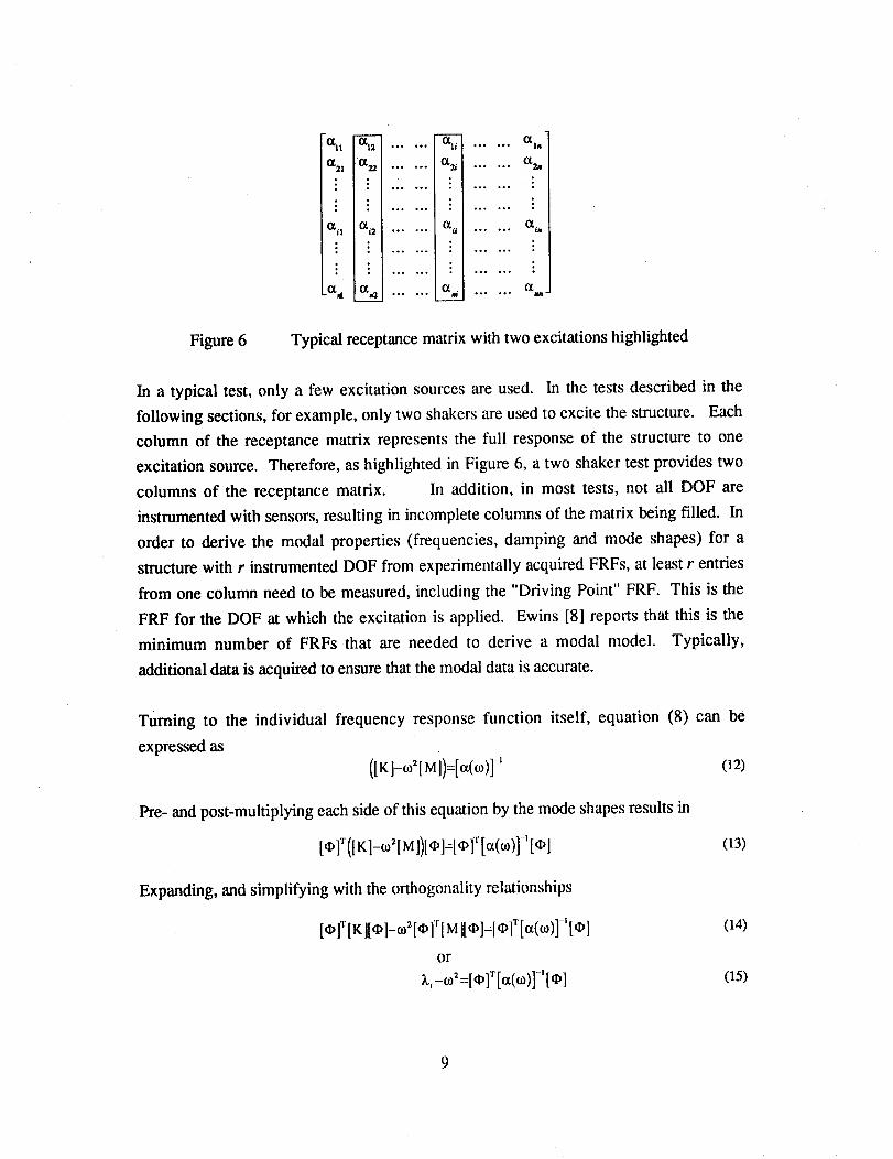
If measurements of the response of the structure at all n DOF for each excitation can be

made, the full receptance matrix is an n x n symmetric matrix of the form shown in

Figure 6.

_11

0_2! Ix=

0_i2

...... _ ...... (_1_

...... (X_ [ ...... _

• . ,, •• .. .°. • , ......

• .• °o. . i ......

...... O_a I ...... O_in

°• ....... •••

• °• °°•

• °° ••• _-

Figure 6 Typical receptance matrix with two excitations highlighted

In a typical test, only a few excitation sources are used. In the tests described in the

following sections, for example, only two shakers are used to excite the structure. Each

column of the receptance matrix represents the full response of the structure to one

excitation source• Therefore, as highlighted in Figure 6, a two shaker test provides two

columns of the receptance matrix• In addition, in most tests, not all DOF are

instrumented with sensors, resulting in incomplete columns of the matrix being filled• In

order to derive the modal properties (frequencies, damping and mode shapes) for a

structure with r instrumented DOF from experimentally acquired FRFs, at least r entries

from one column need to be measured, including the "Driving Point" FRF. This is the

FRF for the DOF at which the excitation is applied• Ewins [81 reports that this is the

minimum number of FRFs that are needed to derive a modal model• Typically,

additional data is acquired to ensure that the modal data is accurate•

Turning to the individual frequency response function itself, equation (8) can be

expressed as

(lz1-o21Ml)=[o_(o)]-' (12)

Pre- and post-multiplying each side of this equation by the mode shapes results in

[OI1([K]__2[M])[O]=101"[_(o)]-'[01 (13)

Expanding, and simplifying with the orthogonality relationships

[_,lTIZl[_]-o_2l,X,lrIMII_,]=[,DIT[=(0_)]-'I'X'I

or

_,--_2=[_1"[_(_)]-' [01

(14)

(15)

The receptance matrix can then be expressed as

]-'

which is simpler to compute than the formulation in equation (11).

individual FRF can now be computed as

(16)

Notice that the

where

%(,o) ,A,,

the mode shape coefficient for mode i at DOFj

the modal constant or residue

(17)

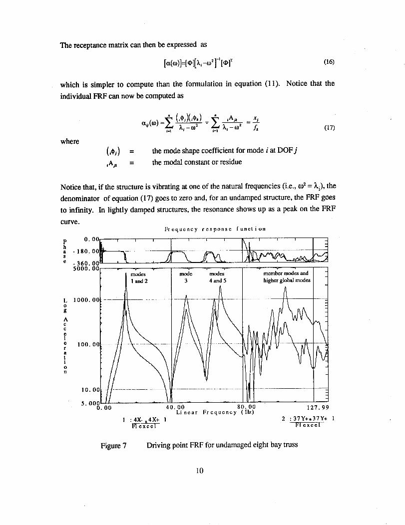
Notice that, if the structure is vibrating at one of the natural frequencies (i.e., o`2 = ki), the

denominator of equation (17) goes to zero and, for an undamped structure, the FRF goes

to inf'mity. In lightly damped structures, the resonance shows up as a peak on the FRF

curve.

Frequency response function

p 0.00 r r r r T _ i 1 1

a - 180. O0 ............................s

e 360. O0

LO

g

AC

C

e

Ie

r

a

.t1

0

n

5000. O0

1000. O0 --

100.00

10.00

5.00

ii i ,!I

"- member mod_es and

higher global modes

00 40. 00 80. O0Linear Frequency (llz)

1 :4X-x4X+ 1 2FI excel

127.99

: 37Y+,37Y+ 1FI excel

Figure 7 Driving point FRF for undamaged eight bay truss

10

Figure 7 shows the two driving point frequency response functions from tests of the

undamaged eight bay truss. Notice that the first two modes are very close together, but

the two FRFs are able to distinguish the modes. The third mode is a torsional mode and

the fourth and fifth modes are the second bending mode pair. Above 80 Hz. the

individual diagonals and longerons begin to vibrate and the next global mode is not easily

discernible among the member modes. As described in the next section, this results in

only the first five modes being available for damage location. Notice, also, that the

phase is also plotted. At each resonance there is a change of phase, and likewise at each

anti-resonance.

FINITE ELEMENT ANALYSIS

Introduction

In the previous section the finite element equations were derived for an n x n structural

system. In this section, application of the Finite Element Method (FEM) dynamic

analysis will be applied to the test article. The eight bay truss was modeled in the I-

DEAS pre-processor SUPERTAB TM, supplied by the Structural Dynamics Research

Corporation (SDRC). The SUPERTAB TM translator was then used to write an input file

for MSC/NASTRAN TM and a normal modes analysis was perfOrmed. As part of the

NASTRAN run the mass and stiffness matrices were output to MATLAB TM [9] readable

files for use in sensitivity studies and for the damage location tests. The finite element

modeling and normal modes results will be presented in this section as a precursor to the

description of the test configuration and results.

Modeling.

SDRC I-DEAS TM was used to model each of the struts and node balls for the eight bay

truss. There are 36 nodes in the truss, resulting in a system with 216 translational and

rotational DOF. The full FEM mass and stiffness matrices are thus 216 x 216 in size.

Because accelerometers only measure translational motion, it is common practice to

reduce the FEM model to include only the x, y and z translational DOF. This was done

for the eight bay truss, resulting in matrices of dimension 108 x 108. The four nodes

cantilevered to the wall were assumed rigidly fixed, thus removing an additional 12 DOF

from the model. The final analysis model thus contains matrices of dimension 96 x 96.

11

The struts were modeled as NASTRAN CBAR elements, each with three translational

DOF at each node. Half of the mass of each beam was lumped at the two nodes

connecting the beam element. Lumped mass elements were used to model the node balls

and the accelerometers. In addition, a lumped mass value was added for the

accelerometer and a percentage of the cable masses, even though an attempt was made to

off load as much of the cable mass as possible in the test. The added stiffness of the

accelerometer cables was considered negligible.

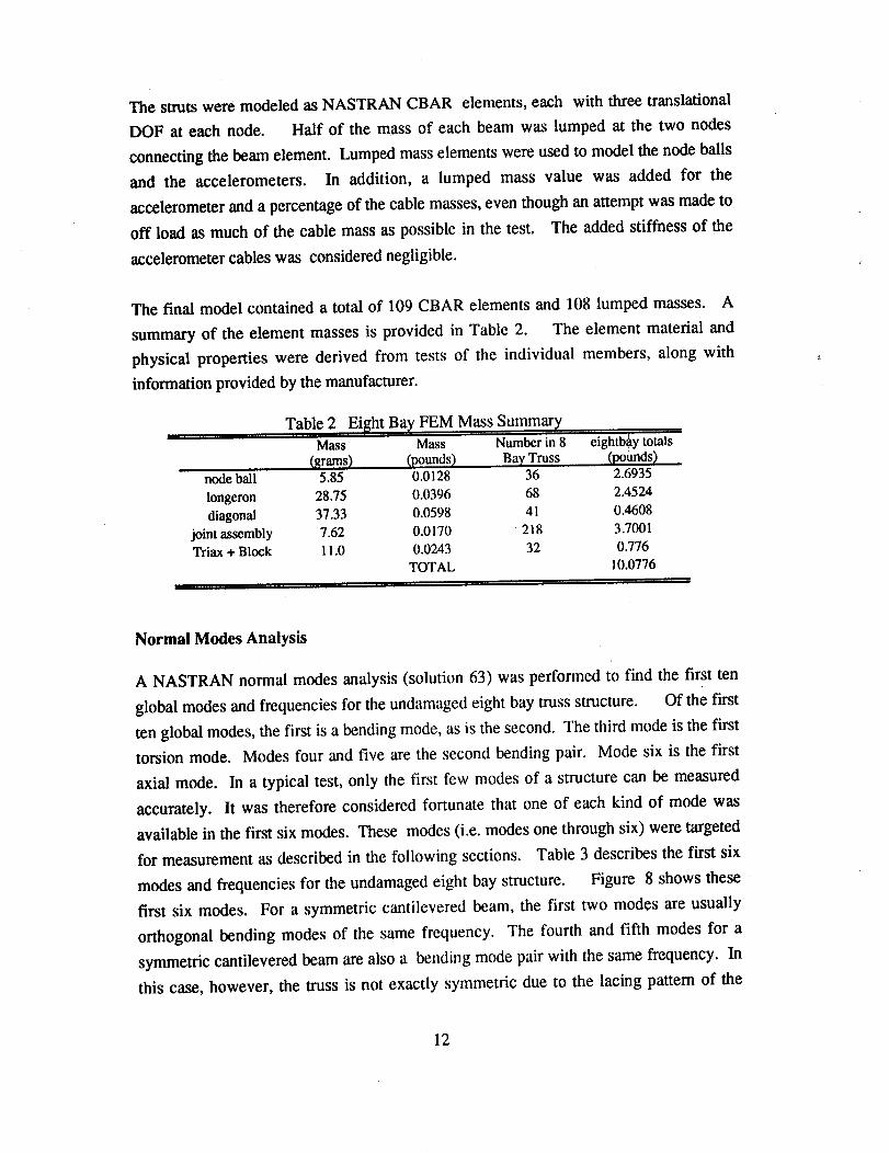
The final model contained a total of 109 CBAR elements and 108 lumped masses. A

summary of the element masses is provided in Table 2. The element material and

physical properties were derived from tests of the individual members, along with

information provided by the manufacturer.

node ball

longerondiagonal

joint assemblyTriax + Block

Table 2 Eight Bay FEM Mass SummaryMass Mass Number in 8 ' eightb/ly totals

_rams) _pounds) Bay Truss _pounds)5.85 0.0128 36 2.6935

28.75 0.0396 68 2.452437.33 0.0598 41 0.4608

7.62 0.0170 218 3.700111.0 0.0243 32 0.776

TOTAL 10.0776

Normal Modes Analysis

A NASTRAN normal modes analysis (solution 63) was performed to find the first ten

global modes and frequencies for the undamaged eight bay truss structure. Of the first

ten global modes, the first is a bending mode, as is the second. The third mode is the first

torsion mode. Modes four and five are the second bending pair. Mode six is the first

axial mode. In a typical test, only the first few modes of a structure can be measured

accurately. It was therefore considered fortunate that one of each kind of mode was

available in the first six modes. These modes (i.e. modes one through six) were targeted

for measurement as described in the following sections. Table 3 describes the first six

modes and frequencies for the undamaged eight bay structure. Figure 8 shows these

first six modes. For a symmetric cantilevered beam, the first two modes are usually

orthogonal bending modes of the same frequency. The fourth and fifth modes for a

symmetric cantilevered beam are also a bending mode pair with the same frequency. In

this case, however, the truss is not exactly symmetric due to the lacing pattern of the

12

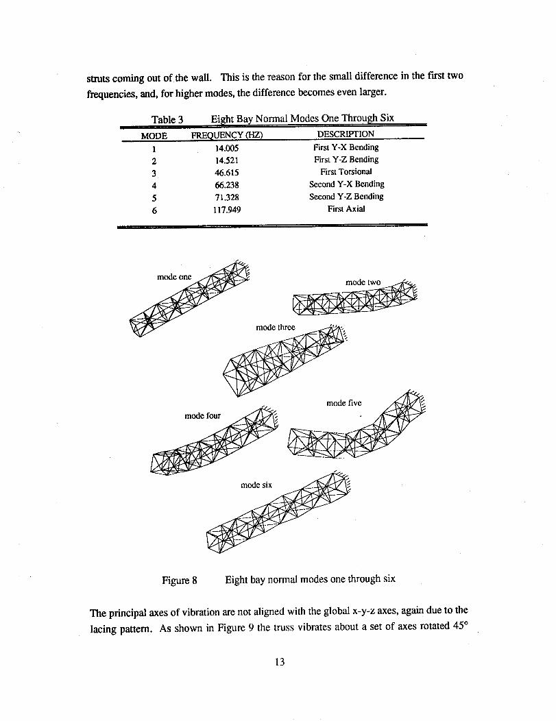
struts coming out of the wall. This is the reason for the small difference in the first two

frequencies, and, for higher modes, the difference becomes even larger.

Table 3 Eight Bay Normal Modes One Through Six

MODE FREQUENCY 0"IZ) DESCRIPTION

1 14.005 First Y-X Bending

2 14.521 First Y-Z Bending

3 46.615 First Torsional

4 66.238 Second Y-X Bending

5 71.328 Second Y-Z Bending

6 117.949 First Axial

mode twoj._

mode__

• /

Figure 8 Eight bay normal modes one through six

The principal axes of vibration are not aligned with the global x-y-z axes, again due to the

lacing pattern. As shown in Figure 9 the truss vibrates about a set of axes rotated 45 °

13

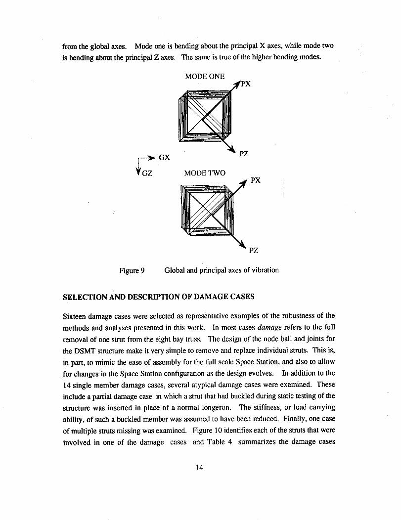
from theglobalaxes. ModeoneisbendingabouttheprincipalX axes,whilemodetwo

isbendingabouttheprincipalZ axes. Thesameis trueof thehigherbendingmodes.

/"

G_Z GX

MODE ONEPX

Z

MODE TWOPX

PZ

Figure 9 Global and principal axes of vibration

SELECTION AND DESCRIPTION OF DAMAGE CASES

Sixteen damage cases were selected as representative examples of the robustness of the

methods and analyses presented in this work. In most cases damage refers to the full

removal of one strut from the eight bay truss. The design of the node ball and joints for

the DSMT structure make it very simple to remove and replace individual struts. This is,

in part, to mimic the ease of assembly for the full scale Space Station, and also to allow

for changes in the Space Station configuration as the design evolves. In addition to the

14 single member damage cases, several atypical damage cases were examined. These

include a partial damage case in which a strut that had buckled during static testing of the

structure was inserted in place of a normal longeron. The stiffness, or load carrying

ability, of such a buckled member was assumed to have been reduced. Finally, one case

of multiple struts missing was examined. Figure 10 identifies each of the struts that were

involved in one of the damage cases and Table 4 summarizes the damage cases

14

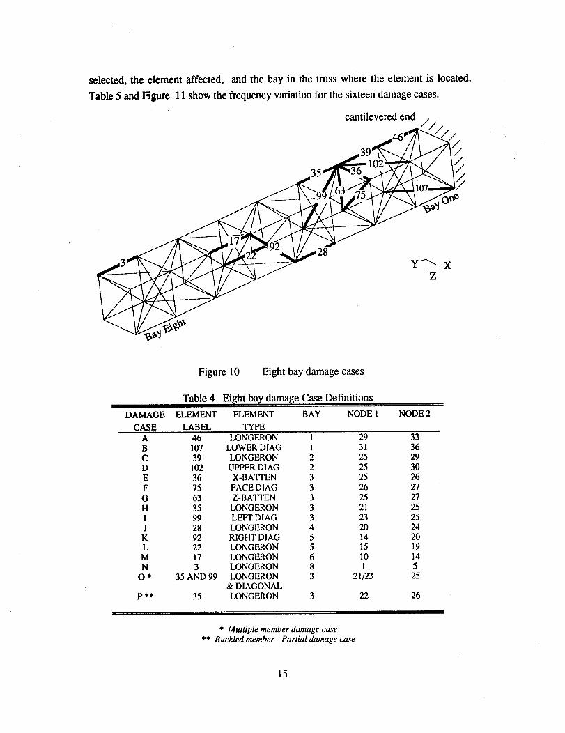
selected, the element affected, and the bay in the truss where the element is located.

Table 5 and Figure 11 show the frequency variation for the sixteen damage cases.

cantilevered end/

Figure 10 Eight bay damage cases

Table 4 Eight bay damage Case Def'mitions

DAMAGE ELEMENT ELEMENT BAY NODE1 NODE2

CASE LABEL TYPE

A 46 LONGERON 1 29 33B 107 LOWER DIAG 1 31 36C 39 LONGERON 2 25 29D 102 UPPER DIAG 2 25 30E 36 X-BATTEN 3 25 26F 75 FACE DIAG 3 26 27G 63 Z-BATTEN 3 25 27H 35 LONG ERON 3 21 25I 99 LEFT DIAG 3 23 25J 28 LONGERON 4 20 24K 92 RIGHT DIAG 5 14 20L 22 LONGERON 5 15 19M 17 LONGERON 6 10 14N 3 LONGERON 8 1 5

O * 35 AND 99 LONGERON 3 21/23 25& DIAGONAL

P ** 35 LONGERON 3 22 26

* Multiple member damage case** Buckled member - Partial damage case

15

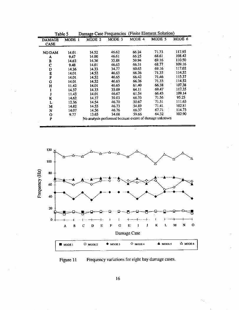
Table 5 Damage Case Frequencies (Finite Element Solution)DAMAGE MODE 1 MODE 2 MODE 3 MODE 4 MODE 5 MODE 6

CASE

NO DAM 14.01 14.52 46.62 66.24 71.33 117.95

A 9.47 14.00 46.61 66.25 68.61 108.42

B 14.63 14.36 35.88 59.94 69.16 110.50

C 9.48 14.01 46.63 66.31 68.77 109.16

D 14.36 14.33 34.77 60.63 69.16 117.02

E 14.01 14.52 46.63 66.26 71.33 114.52

F 14.01 14.52 46.65 66.42 71.46 115.37

G 14.01 14.52 46.63 66.26 71.33 114.52

H 11.42 14.01 46.65 61.40 66.38 107.38

I 14.37 14.33 35.09 64.11 69.47 117.35

J 11.43 14.01 46.67 61.54 66.43 109.14

K 14.62 14.37 39.03 66.33 71.56 95.25

L 12.36 14.54 46.70 50.67 71.51 111.63

M 14.82 14.55 46.73 54.89 71.41 102.81

N 14.07 14.56 46.76 66.37 67.71 114.73

O 9.77 13.65 34.68 59.66 64.32 102.90

P No analysis performed because extent of damage unknown

120

100

80

6O

40

20

....... -+- ...... q- ........ 4 ..... t- .... 4..... t.......... t -_......... I ..... -t-- -- I I I I I

A B C D E F G I1 1 J K L M N O

Damage Case

I • MODEl -D MODE2 • MODE3 <> MODF.4 _k MODE5 _ MODE6

Figure 11 Frequency variations for eight bay damage cases.

16

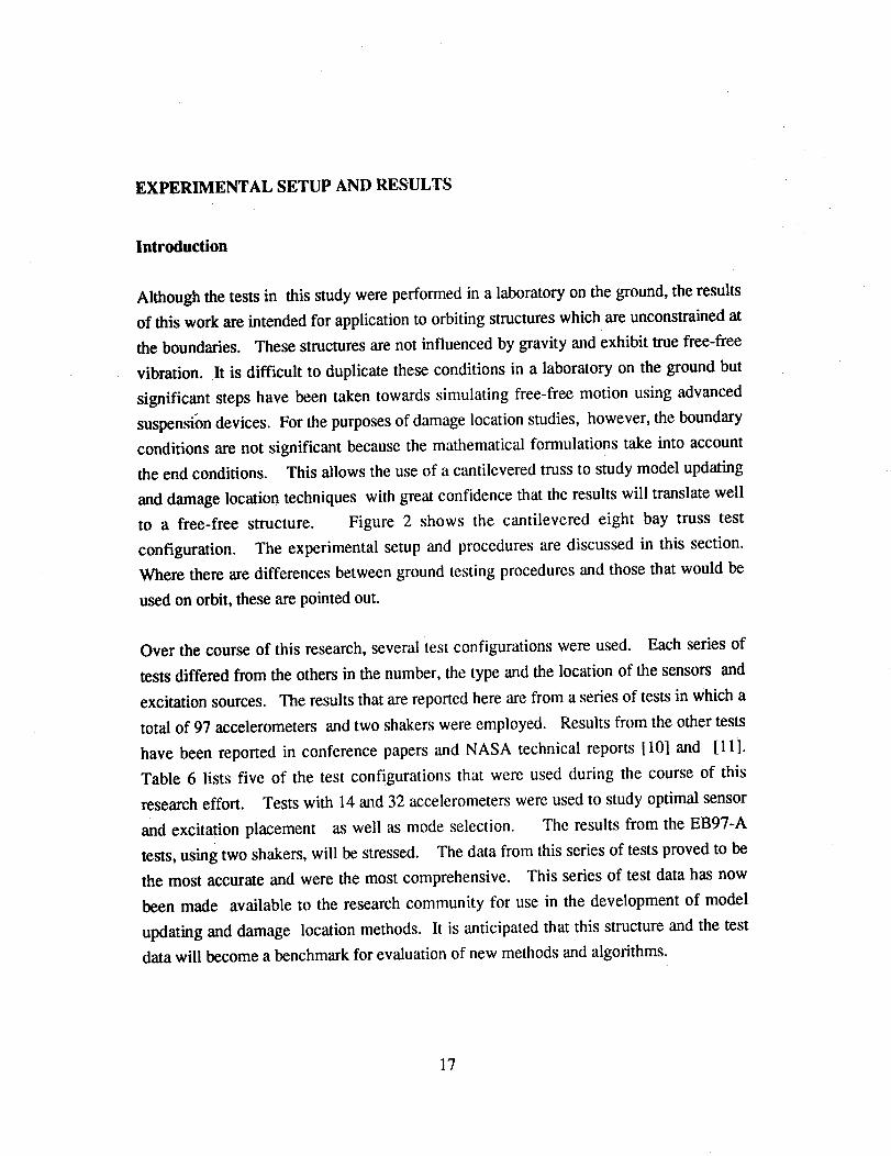
EXPERIMENTAL SETUP AND RESULTS

Introduction

Although the tests in this study were performed in a laboratory on the ground, the results

of this work are intended for application to orbiting structures which are unconstrained at

the boundaries. These structures are not influenced by gravity and exhibit true free-free

vibration. It is difficult to duplicate these conditions in a laboratory on the ground but

significant steps have been taken towards simulating free-free motion using advanced

suspension devices. For the purposes of damage location studies, however, the boundary

conditions are not significant because the mathematical formulations take into account

the end conditions. This allows the use of a cantilevered truss to study model updating

and damage location techniques with great confidence that the results will translate well

to a free-free structure. Figure 2 shows the cantilevered eight bay truss test

configuration. The experimental setup and procedures are discussed in this section.

Where there are differences between ground testing procedures and those that would be

used on orbit, these are pointed out.

Over the course of this research, several test configurations were used. Each series of

tests differed from the others in the number, the type and the location of the sensors and

excitation sources. The results that are reported here are from a series of tests in which a

total of 97 accelerometers and two shakers were employed. Results from the other tests

have been reported in conference papers and NASA technical reports [10] and [11].

Table 6 lists five of the test configurations that were used during the course of this

research effort. Tests with 14 and 32 accelerometers were used to study optimal sensor

and excitation placement as well as mode selection. The results from the EB97-A

tests, using two shakers, will be stressed. The data from this series of tests proved to be

the most accurate and were the most comprehensive. This series of test data has now

been made available to the research community for use in the development of model

updating and damage location methods. It is anticipated that this structure and the test

data will become a benchmark for evaluation of new methods and algorithms.

17

Table 6 Eight Ba_, TestsNUMBER OF NUMBER OF TYPE OF

TEST LABEL ACCELS EXCITERS EXCITATIONEB 14-I 14 1 IMPACTEB 14-A 14 2 BURSTEB32-A 32 2 BURSTEB32-B 32 3 BURSTEB97-A 97 2 BURSTEB97-B 97 3 BURST

Ninety-Seven Accelerometer Test Setup.

The results that are reported here are from a series of tests in which a total of 97

accelerometers were used to measure the acceleration time histories of the truss during

modal testing. Two electromagnetic shakers were used as sources of excitation. In the

following paragraphs, details about the sensor and shaker placement, along with other

specifics about the test configuration, will be presented.

Excitation Placement

Two electromagnetic shakers were used in the EB97-A tests. The shakers selected were

APS Dynamics brand with a + 3 inch stroke. The first shaker was connected at node four

in the negative x direction. The second shaker was placed at node 7 at a 45 ° angle

such that there would be a component of the force in the positive y direction and a

component in the negative z direction. This allowed for excitation of both the torsional

modes and the axial mode, as well as enhancing the bending mode excitation.

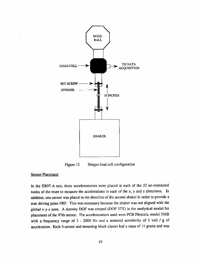
The shakers were connected to the structure through 10 inch long, 0.1 inch diameter

stingers as shown in Figure 12. Each stinger was attached to a PCB model 208-AO2

load cell, which was used to measure the force that was applied to the structure.

Uncorrelated burst random input of about _+0.5 lb maximum force was used in each of

the tests reported here. The burst random signal was generated and controlled by the

signal generation capability in the data acquisition system.

18

NODEBALL

LOAD CELL TO DATA

ACQUISITION

SET SCREW

STINGER

10 INCHES

SHAKER

Figure 12 Stinger-load cell configuration

Sensor Placement

In the EB97-A test, three accelerometers were placed at each of the 32 un-restrained

nodes of the truss to measure the accelerations in each of the x, y and z directions. In

addition, one sensor was placed in the direction of the second shaker in order to provide a

true driving point FRF. This was necessary because the shaker was not aligned with the

global x-y-z axes. A dummy DOF was created (DOF 37Y) in the analytical model for

placement of the 97th sensor. The accelerometers used were PCB Flexcels, model 336B

with a frequency range of 1 - 2000 Hz and a nominal sensitivity of 1 volt / g of

acceleration. Each 3-sensor and mounting block cluster had a mass of 11 grams and was

19

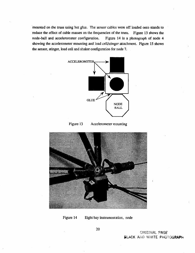
mountedon the truss using hot glue. The sensor cables were off loaded onto stands to

reduce the effect of cable masses on the frequencies of the truss. Figure 13 shows the

node-ball and accelerometer configuration. Figure 14 is a photograph of node 4

showing the accelerometer mounting and load cell/stinger attachment. Figure 15 shows

the sensor, stinger, load cell and shaker configuration for node 7.

GLUE

Figure 13 Accelerometer mounting

Figure 14 Eight bay instrumentation, node

20OR{G!NAL PAGE

_L,ACK ANi_:) WHITE PHOTOGRAPH

BLACK Ai'qO WHITE PHO'iOGRAPH

Figure 15 Eight bay instrumentation, node 7.

Data Acquisition and Test Procedures

For most of the eight bay tests, a sixteen channel GEN RAD 2515 data acquisition system

was used to acquire the acceleration and force time histories and perform the preliminary

signal processing on the data. With only sixteen channels of data being acquired

simultaneously, the time required for a single 97 accelerometer test often exceeded five

hours. Processing of the data added considerably to the overall test time.

Environmental conditions can change dramatically over a period of five hours, resulting

in changes in sensor calibration and possible errors in measurement. Consistency

between data sets was therefore very difficult to achieve.

The EB97-A test was performed using a Zonic 7000 data acquisition system. This

system is capable of handling 256 channels of input simultaneously, thus reducing the

length of a single damage case test to under half an hour. Data acquisition and parameter

estimation for the 16 damage cases took less than 20 hours. The quality and consistency

of the data from one damage case to another is therefore considerably better than the

previous tests. Frequencies, mode shapes and damping ratios for the EB97-A data are

very accurate as will be described in the next section.

21

Following is a description of each of the steps performed in preparation for,

execution of, a typical test.

1. Calibrate accelerometers and load cells

and

At the beginning of the testing process, each of the 97 accelerometers and the

two load cells were subjected to a known input. The resulting voltage output

was divided by the input to provide the actual sensor sensitivity to a unit

input. The calibration constants are used in the signal processing to arrive at

the amplitude and phase of the frequency response functions, and thus the

mode shapes. Accurate frequencies can be obtained with poor calibration

but the mode shape scaling can be severely affected if the accelerometer

calibration constants are inaccurate.

.

.

Sensor calibration could prove to be troublesome for an orbiting structure. In

the lab, accelerometers are calibrated using hand-held vibrators that emit a

signal at a known, constant frequency and amplitude. In space a more

autonomous calibration system will have to be developed so that astronauts

do not need to leave the spacecraft for the calibration process.

Perform system check to verify cable connections and joint tightness.

With a large number of accelerometers it is easy to orient one in the wrong

direction, cross wires from one sensor to another, or have loose connections.

It is critical that a simple test be performed, mode shapes estimated and the

directions and operation of all sensors verified. This can save considerable

time on tracking errors and modifying data after the fact.

Autorange data acquisition channels.

At the beginning of the testing process, a continuous random signal is sent

to the two shakers. The response from each of the load cells and

accelerometers is measured and the full scale voltage (FSV) for each of the

channels adjusted so that all of the signal is within the FSV range. This FSV

is then multiplied by a factor of 2 or 3 to avoid overloads during the data

acquisition process.

22

, Set force levels in shakers and verify uncorrelated forces. Set block size,burst on and off duration, and number of averages.

In the EB97-A tests the shakers were driven by a burst random excitation

generated by the Zonic signal generator capability. Burst random excitation

was selected for these tests because it tends to result in more accurate FRFs

in lightly damped structures than other types of excitation. The signal

generator produces a random mixture of amplitudes and phases for the entire

frequency range of interest (in this case 0 to 128 Hz). A different random

signal is generated and output for several successive cycles. Measurements

are acquired in each cycle and averaged to produce the final FRF. Each

cycle consists of a signal ON time in which the generator sends the two

different random signals to the shakers and an OFF time in which no signal is

transmitted. The total cycle time is determined by the resolution desired.

The resolution is a function of how many spectral lines are used in the

frequency range. This is known as the block size. For the EB97-A tests, a

block size of 4096 was used. This results in 1600 alias free spectral lines or

32 lines per Hz. With such high resolution it is expected that the frequencies

and mode shapes should be extremely accurate.

For a 4096 block size over a 128 HZ range, the total time required by the

analyzer to acquire the data and store it was determined to be 12.5 seconds.

By trial and error the ON time was set at 4.5 seconds and the OFF time at 8.0

seconds. This allowed the entire burst to die out while the response was

being stored before the next cycle was started. 25 averages were used in each

test.

For a structure such as the Space Station, the only source of excitation will be

from the reaction control thruster (RCS) jets. Studies are currently underway

[12] to determine ways to generate pseudo-random excitations using pulsed

firings of the RCS thrusters. Due to data handling and storage considerations

it is unlikely that very large block sizes will be used for on-orbit data

acquisition thus limiting the resolution and accuracy of the measured modes

and frequencies.

23

6. Acquire data.

.

.

Once all parameters have been set and verified, data is acquired. The signal

generator sends out its first cycle and for 4.5 seconds the structure is forced to

vibrate. The response from each of the channels is stored and an FFT is

performed on the time history in the following 8 seconds. Once the data has

been stored the signal generator triggers again, and the process is repeated.

At the end of each cycle the driving point FRFs are displayed on the terminal

along with the coherence function for each force signal. In addition, a

display shows the status of each of the accelerometer channels and monitors

the FSV to ensure that the signal remains within acceptable limits. If the

signal from the sensor goes above the FSV the channel overloads and that

cycle can be rejected from the averaging. Likewise, if the signal is too low

(below 10% of the FSV), the cycle can be rejected. In all of the 16 cases,

only one overload and no underloads occurred.

Examine driving point FRF and at least one other FRF for each set to verify

good data.

Once the 25 cycles are completed and the averaging performed by the

analyzer, the driving point FRFs should be examined to ensure that all of the

modes of interest were excited and that the quality of the data is acceptable.

The coherence function and the cross spectra should also be examined to

ensure that all anomalies can be explained.

Store FRFs and�or acceleration time histories.

Depending on the parameter estimation procedure that is going to be used,

either the FRF's or the time histories should be stored on the hard disk of the

data acquisition system. Reference I131 presents the theory behind a number

of commonly used parameter estimation techniques. In the EB97-A tests,

both time histories and FRFs were stored. The parameters reported in this

work were estimated using the Polyreference technique from the FRFs.

However, the ERA parameter estimation method is likely to be used for

orbiting structures and this method requires time histories. It is anticipated

that the time histories stored from these tests will be used in ERA at a later

date.

24

8. Re-configure truss for next test.

The ease of re-configuring the eight bay truss for different damage cases

made the process very simple. The removed strut from one case is replaced

and the next one taken out within a matter of minutes. In most cases

autoranging between test cases was not performed. Once the new strut was

removed, data was acquired immediately.

Data Reduction and Post-Processing

Frequency Response Functions

An FFT of the time domain data (accelerometer time histories) was performed

automatically by the analyzer in the data acquisition system, transforming it to the

frequency domain. Dividing by the two different inputs from the load cells gives the

frequency response functions corresponding to equation (17). Several FRFs will be

shown in the next section.

Parameter Estimation

The Polyreference parameter estimation technique, as implemented in the I-DEAS

TDAS TM module I141, was used to extract the first five modes from each of the test cases.

At frequencies higher than 75 Hz, the modes of the individual diagonals overlap with the

global truss modes and identifying these global modes becomes very difficult. In some

cases it was possible to obtain accurate frequencies for the sixth mode, but mode shape

extraction was very inaccurate. For this reason, only results for modes one through five

will be reported to maintain consistency in damage location evaluation for all cases. A

detailed description of the Polyreference parameter estimation technique is beyond the

scope of this work. Reference [141 has a detailed derivation and practical details for

correct use of the method. Suffice it to say that the output from the Polyreference

parameter estimation is a set of modal properties consisting of a mode shape coefficient at

each DOF, a damping ratio for each mode and the frequency, in Hz. These modal

properties are output to an I-DEAS Universal file which can be translated using a

FORTRAN code into MATLAB TM readable format.

25

P0st-Processing of Test Mode Shapes.

The mode shapes, that are the end-result of the Polyreference parameter estimation, are

scaled arbitrarily and are not usually orthogonal with respect to the finite element mass

matrix. In order to make them useful in the damage location and model correlation it is

necessary to scale them such that they are orthogonal with respect to the FEM mass

matrix. Each set of eight bay test modes ["V], of dimension 96 x 5 (the extra DOF used

for generating the driving point FRFs is not included in the final modes), was scaled to

unit modal mass

{*}i = _/{V}i[M]{_/}i (18)

If the test data is of good quality, the cross-orthogonality matrix of the scaled modes will

have unit diagonals (this will be true in all cases if equation (18) is used), and very small

off-diagonal terms. If the off-diagonal terms are close to zero, no further processing of

the data is usually required. If the off-diagonal terms are larger than 0.05, an optimal

orthogonalization method such as those described in Reference [151, should be employed

to improve the modes.

26

EIGHT BAY TEST RESULTS

In this section, the results for several interesting damage cases will be presented, along

with comments about all of the tests results. Table 6 and Figure 16 show the test

frequencies for each of the damage cases. Notice that no results are reported for mode

six, as explained earlier.

Table 6 Dama[[e Case Frequencies (From Test)DAMAGE MODE 1 MODE 2 MODE 3 MODE 4 MODE 5

CASENO DAM 13.88 14.48 48.41 64.03 67.46

A 9.50 13.94 48.50 64.08 65.80B 14.52 14.22 36.73 57.28 65.82C 9.50 13.94 48.52 64.16 65.91D 13.47 14.12 35.65 60.18 65.86E 13.90 14.52 48.53 64.31 67.54F 13.91 14.52 48.53 64.41 67.86G 13.91 14.52 48.44 64.34 67.54H 11.39 13.97 48.53 59.90 64.50I 13.21 14.44 36.68 61.35 66.96J 11.42 13.96 48.57 59.91 64.61K 13.46 14.47 41.01 64.41 67.98L 12.29 14.50 48.67 50.65 67.76M 13.73 14.55 48.68 54.76 67.71N 13.98 14.61 48.83 64.20 65.24O 9.86 13.74 36.66 58.86 63.35P 13.83 14.24 48.43 64.03 66.42

0 ..... __m m

°I \/\/ \'7 \'/ \/

0 4-----I- ..... _---ff---4 ........ I----4 ........ t t ...... _..... t....... I...... _....... I-- I I I I

NO A B C D E F G H I J K L M N O P

DamageDamage Case

tl MODE 1 43 MODE 2 * MODE 3 _- MODE 4 -A- MODE 5

Figure 16 Frequency variations for eight bay test cases

27

Undamaged Truss

The first test performed was for the undamaged structure. Figure 17 shows the driving

point frequency response functions for the undamaged structure. The first two modes are

almost indistinguishable from each other. Recall that the frequencies for these modes

from the FEM analysis were separated by only half a Hertz. One of the most critical

observations that can be made from this figure is that the diagonal and longeron modes

begin to interfere with the global modes above 80 Hz. This could not be anticipated from,

the FEM, because the FEM analysis only identifies global modes. Although it is

possible in some of the damage cases to extract the sixth mode (axial) it varies

considerably from test to test. For this reason, modes and frequencies for only the first

five modes were estimated and used in the damage location studies.

5000.00 I --

to00.o0

rFeq_enoy roiponal funatAon

- r--! .... ! I

r I I • - .... _1 t I

i

lOgO0 _ .... _

_OO0O_OQ 40_O0 |O.O0

i_in_ir V_eq_°l_,v I_b

rt*l_*t

ll-rml-l+ 1511_127

+

+

t -

----s

.1. .A .......

121.00

s :)Iy+ e )+Y* t

rlllell

21..PEm-+2 1+:1+,]1

Figure 17 Driving point FRFs. Undamaged truss

28

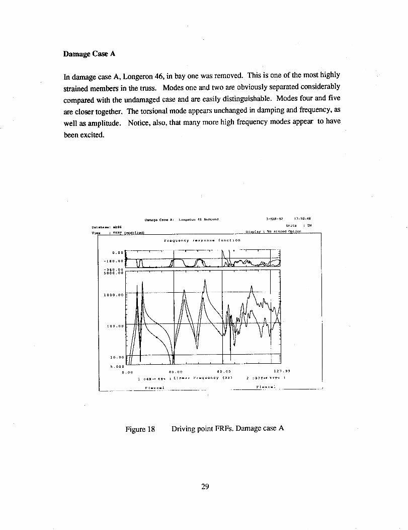
Damage Case A

In damage case A, Longeron 46, in bay one was removed. This is one of the most highly

strained members in the truss. Modes one and two are obviously separated considerably

compared with the undamaged case and are easily distinguishable. Modes four and five

are closer together. The torsional mode appears unchanged in damping and frequency, as

well as amplitude. Notice, also, that many more high frequency modes appear to have

been excited.

Damago Cano A:

Databaaa: abg6

VIQW : TEST _modtflud)

l,ong_ron 46 Rumovod 3-MAR-92 17:50:48

Units : IN

Displa_ : No stored Option

Frequency rosponso function

000[-T _, ................._-,,°.°°! _.:, _-360 O0

5000 O0

1000 O0

100 O0

10 OC

5.000

0.00 40.00

1 .-:-_e--_-_-R_-I Llnoar Froquoncy (Hz)

FIQXCOI

v

I I i t

80.00

/

127.99

2 :-_-_-_-_,_ 1

Flexcel

Figure 18 Driving point FRFs. Damage case A

29

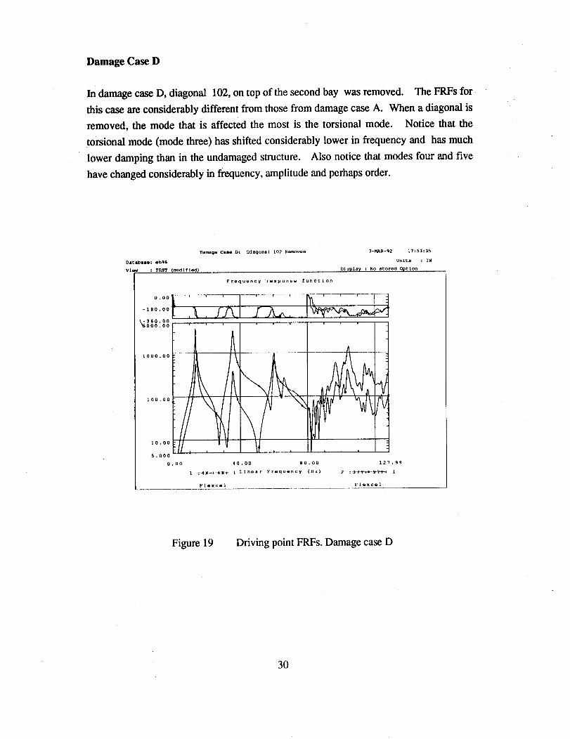
Damage Case D

In damage case D, diagonal 102, on top of the second bay was removed. The FRFs for

this case are considerably different from those from damage case A. When a diagonal is

removed, the mode that is affected the most is the torsional mode. Notice that the

torsional mode (mode three) has shifted considerably lower in frequency and has much

lower damping than in the undamaged structure. Also notice that modes four and five

have changed considerably in frequency, amplitude and perhaps order.

Damage Case D:

Databale: eb96

vlew : TEST Ir_tfled_

Dlaqonal 102 Removed 3-MAR-g2 17:53:35

Units : IN

D_splay : No stored Option

FEQquQncy response function

o00Wr_ __ I .....,-360

_000

1000

100

10

5i

127 . 99

Flexcel _'IeXCQI

Figure 19 Driving point FRFs. Damage case D

30

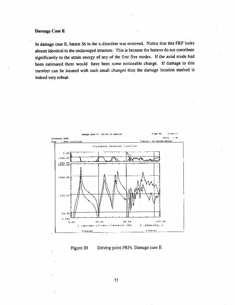
Damage Case E

In damage case E, batten 36 in the x-direction was removed. Notice that this FRF looks

almost identical to the undamaged structure. This is because the battens do not contribute

significantly to the strain energy of any of the first five modes. If the axial mode had

been estimated there would have been some noticeable change. If damage to this

member can be located with such small changes then the damage location method is

indeed very robust.

Damage CasQ E: Batten 36 Removed 17:55:17

Database: ob96 : IN

VIQW : TEST Imodlfled}

3-HAR-92

Units

Display : No stored Option

FrQquency rQsponse funcLlon

-360.00

I10o0.0o

100.00

10.00

i t I5.000

0.00 40.00 80.00

1 .-t_HI--+-4-)PP 1 Linear FrQquoncy (Hz)

FIexcQ1

127 . 99

2 :9-7-Y-H_-_-VA _+ 1

FlexcQ1

Figure 20 Driving point FRFs. Damage case E

31

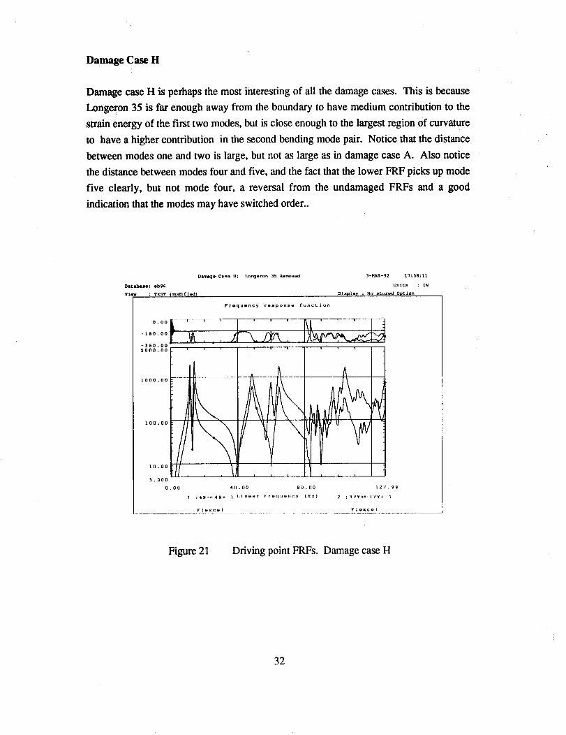
Damage Case H

Damage case H is perhaps the most interesting of all the damage cases. This is because

Longeron 35 is far enough away from the boundary to have medium contribution to the

strain energy of the first two modes, but is close enough to the largest region of curvature

to have a higher contribution in the second bending mode pair. Notice that the distance

between modes one and two is large, but not as large as in damage case A. Also notice

the distance between modes four and five, and the fact that the lower FRF picks up mode

five clearly, but not mode four, a reversal from the undamaged FRFs and a good

indication that the modes may have switched order..

Dar_age Caae H: Longeron 35 I_Qmoved 3-MAR-92 17:58:11

Database: oh96 Units : IN

View : TEST {modlflod_ Dlspla X : No storod Option

Frequency response function

0.00

-180,00

-360,00

5000.00

1000.00

I00.00

10.00

5.000

0.

/

O0

1

F|QxoQL

I I I

I

127

FIQXCQI

.9q

I

Figure 21 Driving point FRFs. Damage case H

32

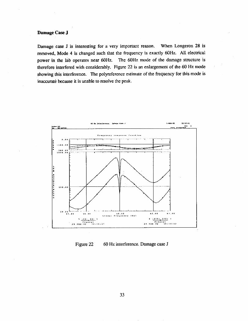
Damage Case J

Damage case J is interesting for a very important reason. When Longeron 28 is

removed, Mode 4 is changed such that the frequency is exactly 60Hz. All electrical

power in the lab operates near 60Hz. The 60Hz mode of the damagestructure is

therefore interfered with considerably. Figure 22 is an enlargement of the 60 Hz mode

showing this interference. The polyreference estimate of the frequency for this mode is

inaccurate because it is unable to resolve the pe_.

to HI |rgtrfe_tnct. D_G* et|i d [-HAR-92 12:12:41

Figure 22 60 Hz interference. Damage case J

33

Damage Case P

In damage case P a longeron that had buckled during static testing, was inserted in the

place of longeron 35. The member was visibly bent and it was anticipated that the load

carrying capacity would be diminished. The FRF, however, appears identical to the

undamaged FRF.

Damaqe Case P: BucklQd Lonqoron 35 3-MAR-92 18:17:09

Database: ab96 Units : IN

View : TZS7 (modtft_l| Dlsplay: No stOrQel Option

F_OqUQnCy rQSpOnSe £unctlon

0.00

-180.00

-360.005000.00

1000.00

I00.00

10.00

5.000

0.00 40.00 80.00

A

1 --_ck_4-_X "_ I Linear Frequency (Hz)

I

127 . 99

F1QXCO1 FIOXCQI

Figure 23 Driving point FRFs. Damage case P

Each of the driving point FRFs from the other damage cases was also examined in detail

before modal parameters were estimated.

34

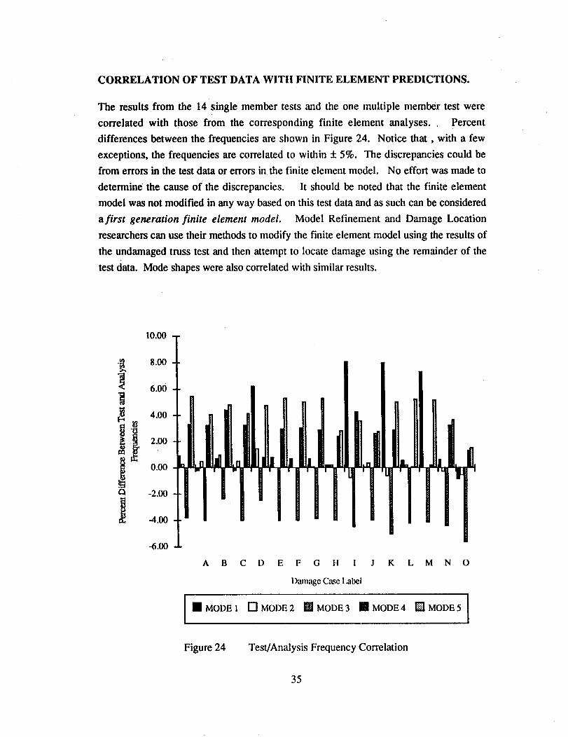
CORRELATION OF TEST DATA WITH FINITE ELEMENT PREDICTIONS.

The results from the 14 single member tests and the one multiple member test were

correlated with those from the corresponding finite element analyses. _ Percent

differences between the frequencies are shown in Figure 24. Notice that, with a few

exceptions, the frequencies are correlated to within + 5%. The discrepancies could be

from errors in the test data or errors in the finite element model. No effort was made to

determine the cause of the discrepancies. It should be noted that the finite element

model was not modified in any way based on this test data and as such can be considered

a first generation finite element model. Model Refinement and Damage Location

researchers can use their methods to modify the finite element model using the results of

the undamaged truss test and then attempt to locate damage using the remainder of the

test data. Mode shapes were also correlated with similar results.

10.00

.,n 8.00c¢1

6.00

2.110

0.00

¢3 -2.00

-4.00

-6.00

A B C D

[] MODE l

Figure 24

E F G H I J K L M

Damage Case Label

[]MODE2 []MODE3 []MODE4

Test/Analysis Frequency Correlation

N O

[] MODE 5 [

35

SUMMARY

A detailed description of a laboratory truss structure has been presented in this report. In

addition, details of the design of the tests that were performed to study damage location

were described. A brief summary of modal testing theory is included for completeness.

A step by step description of the procedures used during testing precedes documentation

and description of some of the results and trends that can be deduced from these results.

The test article is an eight bay section of truss that is one tenth the size and has five times

the dynamics of an early concept of the Space Station Freedom truss. The truss was

subjected to a series of modal tests from which modes and frequencies were extracted.

Frequency response functions from the tests are presented to demonstrate the quality of

the data that can be expected from such tests. Differences between the process of

acquiring modal parameters from a ground vibration test and an on-orbit modal test are

discussed.

The tests presented here and the data collected constitute a significant contribution to the

field of damage detection. The data is available to other researchers and will be used as

a benchmark for development and verification of new model refinement and damage

location techniques.

REFERENCES

.

.

*

.

Kashangaki, T., "Damage Location and Model Refinement for Large FlexibleSpace Structures Using a Sensitivity Based Eigenstructure Assignment Method,"Ph.D Dissertation, University of Michigan, May 1992.

Smith, S.W., and Hendricks, S.L., "Damage Detection and Location in LargeSpace Trusses," AIAA SDM Issues of the International Space Station, ACollection of Technical Papers, Williamsburg, Virginia, April 21-22, 1988, pp. 56-63.

Lim, T.W., "Analytical Model Improvement Using Measured Modes andSubmatrices," AIAA Journal, Vol. 29, No. 6, June 1991, pp. 1015-1018.

Zimmerman , D.C., and Kaouk, M., "Structural Damage Detection Using a

Subspace Rotation Algorithm," 33rd AIAA SDM Conference, Dallas, TX, April13-15, 1992.

36

. Smith, S. W., and McGowan, P.E., "Locating Damaged Members in a TrussStructure Using Modal Data: A Demonstration Experiment," NASA TM-101595,April 1989.

.

.

.

9.

MSC/NASTRAN User's Manual. Version 66. The Macneal-SchwendlerCorporation. 1989.

I-DEAS Finite Element Modeling User's Guide, Structural Dynamics ResearchCorporation, 1990.

Ewins, D.J., M0_laJ Testing: Theory and Practice, Research Studies Press, 1984.

MATLAB TM User's Guide, The MathWorks, Inc., 1991.

10. Kashangaki, T., "On-Orbit Damage Detection and Health Monitoring of LargeSpace Trusses - Status and Critical Issues," Proceedings of the 32nd AIAA SDMConference, Baltimore, MD, April 8-10, 1991. Also published as NASA TM-104045.

11.

12.

Kashangaki, T., Smith, S. W., and Lim, T.W," Underlying Modal Data Issues forDetecting Damage in Truss Structures, " For Presentation at the 33rd AIAA SDMConference, Dallas, TX, April 13-15, 1992.

Cooper, P.A., and Johnson, J.W.," Space Station Freedom On-Orbit ModalIdentification Experiment- An Update", 2nd USAF/NASA Workshop on SystemID and Health Monitoring of Precision Space Structures, Pasadena, CA. March1990.

13. Juang, J., "Mathematical Correlation of Modal-Parameter-Identification MethodsVia System Realization Theory, "International Journal of Analytical andExperimental Modal Analysis," Vol. 2, No. 1, January 1987, pp. 1-18.

14. I-DEAS Test Data Analysis User's Guide, Structural Dynamics Research

Corporation, 1990.

15. Smith, S.W., and Beattie, C.A., "Simultaneous Expansion and Orthogonalization ofMeasured Modes for Structure Identification", Proceedings of the AIAA SDMDynamics Specialist Conference, Long Beach, California, April 5-6, 1990, pp.261-270.

37

Form ApprovedREPORT DOCUMENTATION PAGE OMB NO. 0704-0188

Pub c reportln j burden for this collection of nformation _s estimated Io average 1 hour per resp(inse, rncluding the time for revtewmg instructions, searching existing data sources,

gathering and maintaining the data needed and completing and reviewing the collection ot MlormatIon. Send comments regarding tills burden estimate or any other aspect of thiscollection of information, including suggestions for reducing this burden to Washington Headquarters Services, Directorate for Information Operations and RepOrts, 1215 Jefferson

Oavcs Highway, Suite 1204, Arlington, VA 22202-4302, and to the Office of Management and Budget. P,iperwork Reduction Pro ect (0704-0188), Washington, DC 20503.

1, AGENCY USE ONLY (Leave blank) 2. REPORT DATE 3. REPORT TYPE AND DATES COVERED

May 1992 Technical Memorandum

4. TITLE AND SUBTITLE 5. FUNDING NUMBERS

Ground Vibration Tests of a High Fidelity Truss for

Verification of On Orbit Damage Location Techniques WU 590-14-31-01

6. AUTHOR(S)

Thomas A. L. Kashangaki

7. PERFORMING ORGANIZATION NAME(S) AND ADDRESS(ES)

NASA Langley Research Center

Hampton, VA 23665-5225

9. SPONSORING/MONITORING AGENCY NAME(S) AND ADDRESS(ES)

National Aeronautics and Space Administration

Washington, DC 20546-0001

8. PERFORMING ORGANIZATIONREPORT NUMBER

10. SPON SORING / MONITORINGAGENCY REPORT NUMBER

NASA TM-I07626

11. SUPPLEMENTARY NOTES

Thomas A. L. Kashangaki: Langley Research Center, Hampton, VA

Compilation of data used in AIAA paper #92-2264 presented at the 33rd Structures,

Structural Dynamics & Materials Conference, Dallas, TX, April 13-15, 1992

12a. DISTRIBUTION/AVAILABILITY STATEMENT 12b. DISTRIBUTION CODE

Unqlassified--Unlimited

Subject Category 39

13. ABSTRACT(Max_um200words)

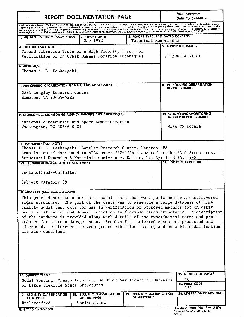
This paper describes a series of modal tests that were performed on a cantilevered

truss structure. The goal of the tests was to assemble a large database of high

quality modal test data for use in verification of proposed methods for on orbit

model verification and damage detection in flexible truss structures. A description

oflthe hardware is provided along with details of the experimental setup and pro-

cedures for sixteen damage cases. Results from selected cases are presented and

discussed. Differences between ground vibration testing and on orbit modal testing

are also described.

14. SUBJECT TERMS

Modal Testlng, Damage Location, On Orbit Verification, Dynamics

of Large Flexible Space Structures

17. ! SECURITY CLASSIFICATIONOF REPORT

U_classified

'NSN_7540-01-280-5500

18. SECURITY CLASSIFICATIONOF THIS PAGE

Unclassified

19. SECURITY CLASSIFICATIONOF ABSTRACT

15. NUMBER OF PAGES

_816. PRICE CODE

A03

20. LIMITATION OF ABSTRAC1

Standard Form 298 (Rev. 2-89)Prescribed by ANSI Std. Z39-18

298-102