ground movement associated with microtunneling
TRANSCRIPT

Louisiana Tech UniversityLouisiana Tech Digital Commons
Doctoral Dissertations Graduate School
Spring 2001
Ground movement associated with microtunnelingZhenyang Duan
Follow this and additional works at: https://digitalcommons.latech.edu/dissertations
Part of the Civil Engineering Commons
INFORMATION TO USERS
This manuscript has been reproduced from the microfilm master. UMI films the text directly from the original or copy submitted. Thus, some thesis and dissertation copies are in typewriter face, while others may be from any type of computer printer.
The quality o f th is reproduction is dependent upon the quality of the copy subm itted. Broken or indistinct print, colored or poor quality illustrations and photographs, print bleedthrough, substandard margins, and improper alignment can adversely affect reproduction.
In the unlikely event that the author did not send UMI a complete manuscript and there are missing pages, these will be noted. Also, if unauthorized copyright material had to be removed, a note will indicate the deletion.
Oversize materials (e.g., maps, drawings, charts) are reproduced by sectioning the original, beginning at the upper left-hand comer and continuing from left to right in equal sections with small overlaps.
Photographs included in the original manuscript have been reproduced xerographically in this copy. Higher quality 6” x 9” black and white photographic prints are available for any photographs or illustrations appearing in this copy for an additional charge. Contact UMI directly to order.
Bell & Howell Information and Learning 300 North Zeeb Road, Ann Arbor, Ml 48106-1346 USA
800-521-0600
Reproduced with permission of the copyright owner. Further reproduction prohibited without permission.

Reproduced with permission of the copyright owner. Further reproduction prohibited without permission.

NOTE TO USERS
This reproduction is the best copy available.
UMI’
Reproduced with permission of the copyright owner. Further reproduction prohibited without permission.

Reproduced with permission of the copyright owner. Further reproduction prohibited without permission.

GROUND MOVEMENT ASSOCIATED WITH MICROTUNNELING
by
Zhenyang Duan, M.S.
A Dissertation Presented in Partial Fulfillment of the Requirement for the Degree of
Doctor o f Philosophy
COLLEGE OF ENGINEERING AND SCIENCE LOUISIANA TECH UNIVERSITY
MAY 2001
Reproduced with permission of the copyright owner. Further reproduction prohibited without permission.

UMI Number: 3003082
___ ®
UMIUMI Microform 3003082
Copyright 2001 by Bell & Howell Information and Learning Company. All rights reserved. This microform edition is protected against
unauthorized copying under Title 17, United States Code.
Bell & Howell Information and Learning Company 300 North Zeeb Road
P.O. Box 1346 Ann Arbor, Ml 48106-1346
Reproduced with permission of the copyright owner. Further reproduction prohibited without permission.

LOUISIANA TECH UNIVERSITY
THE GRADUATE SCHOOL
___________________May, 17,2001____________Date
We hereby recommend that the dissertation prepared under our supervision
by_____________________________ Zhenyang Duan________________________________________________
entitled_________________Ground Movement Associated with Microtunneling_______________________
be accepted in partial fulfillment o f the requirements for the Degree o f
______________ Doctor o f Philosophy in Engineering______________________
Recomrjiflidation concurred in:
— ■
I/jjJJh
Supervisor of Thesis Research ✓
Head of Department
Department
Advisory Committee
Approved
Dean of the Graduate School
GS Form 13 ( 1/00)
Reproduced with permission of the copyright owner. Further reproduction prohibited without permission.

ABSTRACT
Microtunneling is a trenchless technology for construction of pipelines. Its
process is a cyclic pipe jacking operation. Microtunneling has been typically used for
gravity sewer systems in urban areas. Despite its good success record overall, several
large ground settlement cases caused by microtunneling have been reported. Also, in
contrast with large diameter urban tunneling, there are few research projects about the
ground settlement caused by microtunneling.
In this dissertation, the ground settlement caused by microtunneling is studied
using a theoretical approach, empirical approach, numerical simulation approach, and
artificial intelligence approach.
In the theoretical approach, the equivalent ground loss and settlement caused by
concentrated ground loss have been used to drive the ground settlement profile. In the
empirical approach, the ground settlement caused by large diameter tunneling case
histories is used. In the numerical approach, FLAC3D software, a commercially available
finite difference code, is used to simulate the ground settlement caused by
microtunneling. In the artificial intelligence approach, a three-layer back propagation
neural network is developed to predict the ground settlement caused by microtunneling
using the numerical simulation results.
It is found that the neural network developed as part o f this thesis work provides a
means o f rapid prediction o f the surface ground settlement curve based on the soil
iii
Reproduced with permission of the copyright owner. Further reproduction prohibited without permission.

parameters, project geometry and estimated ground loss. This prediction matches
FLAC3D results very well over the full range o f parameters studied and has a reasonable
correspondence to the field results with which it was compared.
iv
Reproduced with permission of the copyright owner. Further reproduction prohibited without permission.

APPROVAL FOR SCHOLARLY DISSEMINATION
The author grants to the Prescott Memorial Library o f Louisiana Tech University the right to
reproduce, by appropriate methods, upon request, any or all portions o f this Thesis. It is understood that
“proper request” consists o f the agreement, on the part o f the requesting party, that said reproduction is for
his personal use and that subsequent reproduction will not occur without written approval o f the author o f
this Thesis. Further, any portions o f the Thesis used in books, papers, and other works must be appropriately
referenced to this Thesis.
Finally, the author o f this Thesis reserves the right to publish freely, in the literature, at any time,
any or all portions o f this Thesis.
Date
Author
GS Form 14 2/97
Reproduced with permission of the copyright owner. Further reproduction prohibited without permission.

DEDICATION
To my wonderful wife Qiaoyu
vi
Reproduced with permission of the copyright owner. Further reproduction prohibited without permission.

TABLE OF CONTENTS
A BSTR A CT............................................................................................................................... iii
D ED ICA TIO N ........................................................................................................................... vi
L IS T O F TABLES.....................................................................................................................x
L IST OF FIG U R ES................................................................................................................ xii
A CK N O W LED G EM EN TS................................................................................................. xvi
C h ap te r 1 IN TRO D U CTIO N............................................................................................ 1
1.1 General Description o f Microtunneling................................................................. 1
1.2 Ground Settlement Associated with Microtunneling........................................... 2
1.3 Research N eed.......................................................................................................... 4
C h a p te r 2 THEORETICAL APPROACH...................................................................... 6
2.1 Excavation Face Stability....................................................................................... 7
2.2 Equivalent Ground L o ss ..........................................................................................92.2.1 Ground Loss Ahead of the Microtunneling Face................................112.2.2 Ground Loss Over the Shield................................................................ 152.2.3 Ground Loss Due to the Tail Void........................................................16
2.3 Ground Movement Due to Concentrated Ground Loss..................................... 172.3.1 Infinite M edium ..................................................................................... 202.3.2 Image Sink: Paved Half-Space............................................................ 222.3.3 Free Surface............................................................................................242.3.4 Surface M ovements...............................................................................26
2.4 Ground Movement Associated with Microtunneling........................................ 28
C h ap te r 3 EM PIRICAL A PPR O A C H ...........................................................................33
C h a p te r 4 NUMERICAL APPROACH 3 8
vii
Reproduced with permission of the copyright owner. Further reproduction prohibited without permission.

4.1 FL AC30 Software.................................................................................................. 38
4.2 Basic Definitions o f FLAC3D Terms (after FLAC3D Menu)............................. 41
4.3 Intrinsic Deformability Properties.......................................................................43
4.4 Modeling Procedure.............................................................................................. 44
4.5 Selection of Boundary and Zones........................................................................464.5.1 Selection of Boundary Condition.........................................................464.5.2 Selection of Pipe Material.....................................................................50
4.6 Effect of Bulk Modulus and Shear Modulus......................................................554.6.1 Effect o f Bulk Modulus on Extent o f Settlement............................... 554.6.2 Effect o f Shear Modulus on Extent o f Settlement............................. 554.6.3 Effect of Bulk and Shear Modulus on
Magnitude of Displacement................................................................. 56
4.7 Effect of Elastic Modulus, Poisson’s Ratio,Cohesion, Friction Angle and Dilation Angle....................................................62
4.7.1 Effect o f Young’s modulus.................................................................. 624.7.2 Effect of Poisson’s R atio ......................................................................654.7.3 Effect of Cohesion................................................................................ 684.7.4 Effect o f Friction Angle........................................................................714.7.5 Effect o f Dilation Angle........................................................................714.7.6 Effect o f Microtunneling Depth........................................................... 764.7.7 Effect o f Product Pipe Radius.............................................................. 76
4.8 Comparisons Between Case History Data and Simulation Results..................78
C h ap te r 5 ARTIFICIAL INTELLIGENCE APPROACH........................................80
5.1 Introduction to Neural Networks.........................................................................80
5.2 Biological Neural Networks (Discussion after Lin, 1995)............................... 83
5.3 Fundamental Feature o f Neural Networks.......................................................... 85
5.4 Feed Forward Multilayer Neural Networks........................................................875.4.1 Activation function............................................................................... 895.4.2 Back Propagation.................................................................................. 905.4.3 Learning Factors o f Back Propagation............................................... 98
5.4.3.1 Initial Weights........................................................................985.4.3.2 Learning Constant (Learning Rate).....................................985.4.3.3 Cost Functions.......................................................................99
viii
Reproduced with permission of the copyright owner. Further reproduction prohibited without permission.

5.4.3.4 Momentum...........................................................................1005.4.3.5 Number of Hidden Nodes.................................................. 1015.4.3.6 Local Minimum............... 1025.4.3.7 Local Minima Happen Easily............................................ 1025.4.5.8 Simulated Annealing...........................................................1065.4.3.9 Choosing the Annealing Parameters..................................107
5.5 Neural Network Used in This Research............................................................ 1085.5.1 Training Set Used to Train Neural Network................................... 109
5.5.1.1 Initial Weight.......................................................................1145.5.1.2 Number of Hidden Layers..................................................1165.5.1.3 Desired Output D ata........................................................... 1165.5.1.4 Local Minimum.................................................................. 117
5.6 Results.................................................................................................................. 119
5.7 Case Histories..................................................................................................... 128
C hap ter 6 CONCLUSIONS & RECOMMENDATIONS........................................ 131
C hap ter 7 FURTHER W ORK.......................................................................................134
7.1 Measurement o f Ground Loss............................................................................1347.2 Prediction of Ground Settlement in Real Time................................................ 135
REFEREN CES..................................................................................................................... 137
APPENDIX A GEND AT A. JAV A .................................................................................... 140
APPENDIX B DATAFILEGEN.JAVA........................................................................... 144
APPENDIX C READLOG.JAVA.................................................................................... 153
APPENDIX D LEASTSQUARE.JAVA........................................................................... 159
APPENDIX E ANN.JAVA................................................. 165
APPENDIX F CONNECT. JAV A ..................................................................................... 188
APPENDIX G FLAC30 INPUT DATA F IL E ................................................................ 191
ix
Reproduced with permission of the copyright owner. Further reproduction prohibited without permission.

LIST OF TABLES
Table 4.1: FLAC3D Constitutive Models (after FLAC3D Menu).........................................40
Table 4.2 Vertical Soil Displacements on the Ground Surface............................................50
Table 4.3 Mechanical Property o f A36 Steel and HDPE...................................................... 51
Table 4.4 Selected Elastic Constants and Strength Propertiesfor Soils [Oritz et al., 1986].................................................................................... 52
Table 4.5 Ground Displacement (meter) for Different Types of Soil.................................. 54
Table 4.6 Vertical Ground Surface Displacement (meter) for Different Bulk M oduli 60
Table 4.7 Horizontal Ground Surface Displacement (meter) forDifferent Bulk M oduli.............................................................................................60
Table 4.8 Vertical Ground Surface Displacement (meter) forDifferent Shear M oduli............................................................................................61
Table 4.9 Horizontal Ground Surface Displacement (meter) forDifferent Shear M oduli............................................................................................61
Table 4.10 Vertical Ground Surface Displacement (meter) forDifferent Young’s Modulus.................................................................................. 64
Table 4.11 Horizontal Ground Surface Displacement (meter) forDifferent Young’s Modulus ............................................................................64
Table 4.12 Vertical Ground Surface Displacement (meter) forDifferent Poisson Ratio...........................................................................................67
Table 4.13 Horizontal Ground Surface Displacement (meter) forDifferent Poisson Ratio..........................................................................................67
Table 4.14 Vertical Ground Surface Displacement (meter) forDifferent Cohesion................................................................................................. 70
Reproduced with permission of the copyright owner. Further reproduction prohibited without permission.

Table 4.15 Vertical Ground Surface Displacement (meter) forDifferent Cohesion.................................................................................................70
Table 4.16 Vertical Ground Surface Displacement (meter) forDifferent Friction A ngle....................................................................................... 73
Table 4.17 Horizontal Ground Surface Displacement (meter) forDifferent Friction A ngle....................................................................................... 73
Table 4.18 Vertical Ground Surface Displacement (meter) forDifferent Dilation A n g le ...................................................................................... 75
Table 4.19 Horizontal Ground Surface Displacement (meter) forDifferent Dilation A n g le ...................................................................................... 75
Table 5.1 Range of Mircotunneling Properties....................................................................111
Table 5.2 Range of Soil Properties....................................................................................... 111
Table 5.3 Ground Settlement Data o f FLAC30 and Neural Networks...(Test Data 1 ).... 120
Table 5.4 Ground Settlement Data o f FLAC30 and Neural Networks...(Test Data 2 ) .... 121
Table 5.5 Ground Settlement Data o f FLAC30 and Neural Networks (Test Data 3 ) .... 122
Table 5.6 Ground Settlement Data o f FLAC30 and Neural Networks (Test Data 4 ) .... 123
Table 5.7 Ground Settlement Data o f FLAC30 and Neural Networks (Test Data 5 ) .... 124
Table 5.8 Ground Settlement Data o f FLAC30 and Neural Networks (Test Data 6 ) .... 125
Table 5.9 Ground Settlement Data o f FLAC30 and Neural Networks (Test Data 7 ) .... 126
Table 5.10 Ground Settlement Data o f FLAC30 and Neural Networks (Test Data 8) ....127
xi
Reproduced with permission of the copyright owner. Further reproduction prohibited without permission.

LIST OF FIGURES
Figure 1.1 Microtunneling System ..........................................................................................3
Figure 1.2 Two Typical Patterns of Failure............................................................................. 4
Figure 2.1 Face Stability M odel............................................................................................... 8
Figure 2.2 Simulation o f Loss o f Ground (The Total Gap Parameter)................................11
Figure 2.3 Dimensionless Axial Displacement Q. (After Lee, 1992)..................................13
Figure 2.4 Dimensionless Axial Displacement Ahead o f Microtunneling Face withVarious Ka Conditions, (after Lee, 1992)............................................................14
Figure 2.5 Steps in Analysis....................................................................................................18
Figure 2.6 Point Sink: Infinite Medium................................................................................. 21
Figure 2.7 Point Sink: Cartesian Co-ordinates......................................................................22
Figure 2.8 Point Sink-Negative Image: (a) Three Dimensions (b) Two Dimensions 23
Figure 2.9 Point Sink: Surface Shear Stresses.......................................................................25
Figure 2.10 Point Sink: Final Surface Displacement............................................................ 28
Figure 2.11 Ground Deformation Pattern and Ground Loss Boundary Conditions..........30
Figure 2.12 Vertical Ground Movement................................................................................ 32
Figure 3.1 Surface Settlement Trough................................................................................... 33
Figure 3.2 Short-Term and Long-Term (Consolidation)Settlements at Ground Surface.............................................................................. 35
Figure 4.1 Domain for FIac3D Simulation — Half Symmetry............................................. 44
Figure 4.2 Boundary Conditions for Flac3D Analysis — Half Symmetry..........................45
xii
Reproduced with permission of the copyright owner. Further reproduction prohibited without permission.

Figure 4.3 Flac3d Grid — Half Symmetry.............................................................................. 45
Figure 4.4 Model Showing Locations of Ground Surface Points................. 47
Figure 4.5 Ground Settlement Trough at D = 5H..................................................................48
Figure 4.6 Ground Settlement Trough at D = 6H ..................................................................48
Figure 4.7 Ground Settlement Trough at D = 7H..................................................................49
Figure 4.8 Ground Settlement Trough at D = 8H..................................................................49
Figure 4.9 Comparison of Soil Displacement for Different Boundary Conditions........... 50
Figure 4.10 Vertical Displacement at Ground Surface for Different Pipe M aterials 52
Figure 4.11 Simulated Ground Movement is Different Soil Type (See Table 4.4for soil type description)......................................................................................53
Figure 4.12 Variation o f Ground Surface Settlement with Bulk Modulus......................... 57
Figure 4.13 Variation of Ground Surface Horizontal Displacement withBulk M odulus.......................................................................................................57
Figure 4.14 Variation of Ground Surface Settlement with Shear Modulus........................ 58
Figure 4.15 Variation of Ground Surface Horizontal Displacement withShear Modulus......................................................................................................58
Figure 4.16 (a) Vector and (b) Contour Plot of Soil Displacement.....................................59
Figure 4.17 Variation of Ground Surface VerticalDisplacement with Young’s Modulus...............................................................63
Figure 4.18 Ground Surface Horizontal Displacement forDifferent Young’s Modulus............................................................................... 63
Figure 4.19 Variation of Ground Surface VerticalDisplacement with Poisson’s Ratio....................................................................66
Figure 4.20 Variation o f Ground Surface HorizontalDisplacement with Poisson’s Ratio...................................................................66
Figure 4.21 Variation o f Ground Surface Vertical Displacement with Cohesion............. 69
Figure 4.22 Variation of Ground Surface Horizontal Displacement with Cohesion.........69
xiii
Reproduced with permission of the copyright owner. Further reproduction prohibited without permission.
Figure 4.23 Variation o f Ground Surface Vertical Displacement with Friction Angle.....72
Figure 4.24 Variation o f Ground Surface HorizontalDisplacement with Friction A ng le .....................................................................72
Figure 4.25 Variation o f Ground Surface Vertical Displacement with Dilation Angle ....74
Figure 4.26 Variation o f Ground Surface HorizontalDisplacement with Dilation A ngle.....................................................................74
Figure 4.27 Maximum Vertical Displacement at Ground Surface versesMicrotunneling Depth........................................................................................... 76
Figure 4.28 Variation o f Vertical Displacement with Product Pipe Radius....................... 77
Figure 4.29 Variation o f Horizontal Displacement with Product Pipe Radius...................77
Figure 4.30 Observed and Predicted SurfaceSettlement — Barcelona Subway Network.........................................................78
Figure 4.31 Observed and Predicted Surface Settlement — Green Park Tunnel, U.K........79
Figure 5.1 A Simple Artificial Neuron....................................................................................81
Figure 5.2 A Very Simple Neural Network............................................................................ 82
Figure 5.3 Biological N euron...................................................................................................83
Figure 5.4 Single-Layer Feed Forward Neuron Network......................................................86
Figure 5.5 A Multilayer Neural Network............................................................................... 87
Figure 5.6 Recurrent Neural N etw ork.....................................................................................87
Figure 5.7 A Single Neural in Hidden Layer..........................................................................88
Figure 5.8 Four-Layer Feed Forward Neural Network..........................................................89
Figure 5.9 Three-Layer Back Propagation Network.............................................................. 92
2Figure 5.10 Bipolar Sigmoid Function f ( x ) = ------— — 1 ................................................... 97
1 -t-e
X IV
Reproduced with permission of the copyright owner. Further reproduction prohibited without permission.

Figure 5.11 Gradient Descent on a Simple Quadratic Surface.......................................... 101
Figure 5.12 A Typical Weight Surface Cross Section..............................:.........................103
Figure 5.13 A Local Minimum in Gradient Learning......................................................... 104
Figure 5.14 Genetic Operations on a Three-Letter Alphabet of {a,b,c} (a) Crossover Swaps Strings at a Crossover Point, (b) Inversion Reverses the Order of Letters in Substring, (c) Mutation Changes a Single Element...................... 105
Figure 5.15 Structure o f Neural Network Used to Predict the Ground Settlement 109
Figure 5.16 Logistic Function...............................................................................................113
Figure5.17 Ground Settlement Result o f FLAC3D and Neural Network (Test Data 1) ..120
Figure 5.18 Ground Settlement Result o f FLAC3D and Neural Network (Test Data 2) ..121
Figure 5.19 Ground Settlement Result of FLAC3D and Neural Network (Test Data 3) ..122
Figure 5.20 Ground Settlement Result o f FLAC30 and Neural Network (Test Data 4) ..123
Figure 5.21 Ground Settlement Result o f FLAC30 and Neural Network (Test Data 5) ..124
Figure 5.22 Ground Settlement Result of FLAC30 and Neural Network (Test Data 6) ..125
Figure 5.23 Ground Settlement Result o f FLACJ° and Neural Network (Test Data 7) ..126
Figure 5.24 Ground Settlement Result of FLAC30 and Neural Network (Test Data 8) ..127
Figure 5.25 Ground Settlement in Sand............................................................................... 129
Figure 5.26 Ground Settlement in Clay............................................................................... 129
Figure 5.27 Ground Settlement in Clay Gravel...................................................................130
X V
Reproduced with permission of the copyright owner. Further reproduction prohibited without permission.

ACKNOWLEDGMENTS
I would like to express my sincere appreciation to ail those individuals who
provided me with guidance and assistance in the preparation of this thesis. Heartfelt
thanks are extended to Dr. Raymond Sterling for serving as the major advisor on this
thesis. His guidance and assistance in the advice, time, and support will forever be
remembered and appreciated. I would also like to thank Dr. Robert McKim, Dr. Paul
Hadala, Dr. David Hall, and Dr. William Jordan for serving as advisory committee
members o f this thesis. Their willingness to assist in reviewing this thesis is sincerely
appreciated. Further acknowledgment is extended to Dr. Mckim and Dr. Hadala for their
additional advice and assistance in my research work.
I would like to thank College o f Engineering and Science of Louisiana Tech
University and Trenchless Technology Center for providing financial support throughout
my research.
Finally, special thanks go to my wife, Qiaoyu Lu, whose love, understanding, and
support encouraged me to complete this thesis.
xvi
Reproduced with permission of the copyright owner. Further reproduction prohibited without permission.

CHAPTER 1
INTRODUCTION
1.1 General Description of Microtuneling
Microtunneling is a trenchless technology for construction of pipelines to close
tolerances for line and grade. Microtunneling installations are typically for gravity
sewers, although other specialized projects have been constructed using this method. The
method was developed in the 1970s in Japan, refined in Germany and the United
Kingdom, and made its debut in the United States in 1984 [Bennett 1995].
No universally accepted definition o f microtunneling exists, but it can be
described as a remotely controlled, guided pipe-jacking that provides continuous support
to the excavation face. The guidance system usually consists o f a laser mounted in the
jacking pit as a reference with a target mounted inside the microtunneling machine’s
articulated steering head.
The microtunneling process is a cyclic pipe jacking operation. The
microtunneling machine is pushed into the earth by means o f hydraulic jacks carefully
mounted and aligned in the jacking shaft. As the jacks are fully extended, the machine is
pushed out o f the pit, and the jacks are then retracted. A product pipe or casing is then
inserted between the jacking ring and the microtunneling machine or previously jacked
pipe, necessary connections are made, and the pipe and machine are advanced another
1
permission of the copyright owner. Further reproduction prohibited without permission.

drive stroke. This cycle is repeated until the completion point (a reception shaft) is
reached.-
There are two primary types o f microtunneling system - auger and slurry - defined
by the method o f spoil removal. These operation systems differ in their degree o f control
o f ground conditions at the face. The slurry system is generally capable of a more precise
control. The slurry system can handle higher groundwater and unstable ground
conditions, but there is the disadvantage o f added mechanical complexity and cost. In
addition, production rates may be slightly lower for slurry machines. Auger machines
have limitations on the length and diameter o f installed pipelines due to the power
requirements for turning the auger and head. Both auger and slurry systems consists o f
five independent subsystems: (1) Mechanized excavation system; (2) Propulsion or
jacking system; (3) Spoil removal system; (4) Guidance and control system; and (5) Pipe
lubrication system. Figure 1.1 shows a typical microtunneling system.
1.2 Ground Settlement Associated with Microtunneling
The ground movement associated with microtunneling is mainly a result o f loss of
ground during tunneling and consolidating compressible soils due to dewatering. During
microtunneling, loss o f ground may be associated with soil squeezing, running, or
flowing into the heading; losses due to the size o f overexcavation; and losses due to
steering adjustments. The actual magnitude o f these losses is largely dependent on the
type and strength o f the ground, groundwater conditions, size and depth o f the pipe,
equipment capabilities, and the skill o f the contractor in operating and steering the
machine. Sophisticated microtunneling equipment that has the capability to exert a
permission of the copyright owner. Further reproduction prohibited without permission.

3
stabilizing pressure at the tunnel face, equal to that o f the in-situ soil and groundwater
pressures, will minimize loss o f ground and surface settlement without the need of
dewatering.
Slurry Tank
Slurry Jet Hoses
Target Plate Steering CylinderDrive Shaft
Conical CrusherBy-pass ValveEntrance
RingSeal
Sluny Return Pipes
Laser
Figure 1.1 Microtunneling System
During microtunneling through soft water-bearing ground, the excavation face
becomes unstable when the soil lacks sufficient cohesion. A temporary support is
required to maintain ground stability in the working area, and a slurry microtunneling
system is widely used to provide this support. In a slurry shield, the temporary support is
provided by a pressurized mixture o f bentonite clay and water. Because o f the high
viscosity o f the slurry, the risk of an uncontrolled escape o f fluid by leakage is generally
reduced. As the slurry is only slightly heavier than water, the excess fluid pressure in the
invert is small. The risk o f an upheaval o f ground, therefore, is eliminated as well. In the
Reproduced with permission of the copyright owner. Further reproduction prohibited without permission.

last decade, slurry-shield tunneling has been applied successfully worldwide on a large
number o f projects.
Figure 1.2 shows schematically two typical patterns o f failure. In the first case,
major soil movements are restricted to a zone close to the heading. The cave-in o f the
ground may form a cavity above the pipe permanently, or it may cause a collapse later. In
the second case, the collapse propagates towards the surface creating a chimney, and
sometimes a crater, on the ground surface. The heading failure then results in excessive
subsidence and possible damage to overlying structures.
More cost effective and less disruptive methods o f installing underground utilities
are key components in creating better utility systems, and they are the first step in the life
cycle o f a new underground utility service. Although a number o f methods for installing
underground utilities exist, there are several crosscutting technology improvements
needed that would impact all such systems. The underground construction industry has
changed radically in the past 20 years, adopting a number o f advanced technology
excavation and guidance systems. Microtunneling is one o f such new technology. This
Figure 1.2 Two Typical Patterns of Failure
1.3 Research Need
permission of the copyright owner. Further reproduction prohibited without permission.

5
change in the nature of the industry (available hardware and receptivity to advanced
methods) provides the path through which further radical changes in utility installation
can be deployed in the industry. There are many research papers about ground settlement
caused by larger diameter tunnel and underground space excavation, but few about
ground settlement caused by microtunneling. Although some aspects o f microtunneling
are similar to large diameter tunneling, microtunneling is a significantly different
technique.
Reproduced with permission of the copyright owner. Further reproduction prohibited without permission.

CHAPTER 2
THEORETICAL APPROACH
In the past 20 years, significant advances have been made in procedures for
evaluating and controlling ground movements around tunnels in soil. Ground movements
are routinely measured on tunnel projects in order to pinpoint the cause o f ground loss
around the advancing tunnel heading and to determine the magnitude o f ground
movements that will develop at nearby structures. Such observations have resulted in
better control o f the tunneling process and have led to an improved understanding o f
ground behavior.
Despite improvements in tunneling and ground control procedures such as those
previously noted, control o f ground movements during tunneling is often difficult to
achieve, particularly when variable ground conditions result in sudden changes along the
length o f the tunnel or across the tunnel face. Improvements are being made in tunnel
shields (microtunneling machine), but a universal machine does not exist. In fact, many
current machines and shields are very sensitive to variations in ground conditions.
Therefore, it is important to obtain as complete a picture o f the ground settlement as
possible prior to selecting and installing the microtunneling machine.
6
with permission of the copyright owner. Further reproduction prohibited without permission.
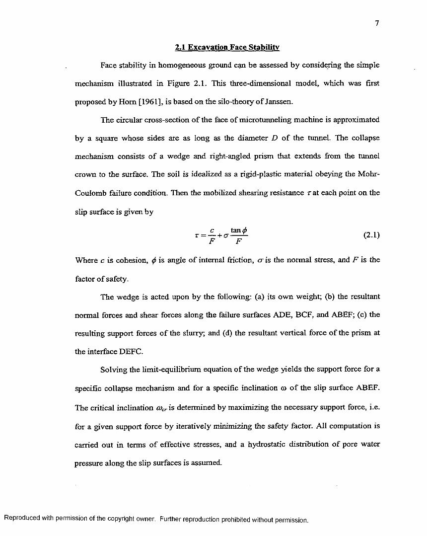
2.1 Excavation Face Stability
Face stability in homogeneous ground can be assessed by considering the simple
mechanism illustrated in Figure 2.1. This three-dimensional model, which was first
proposed by Horn [1961], is based on the silo-theory o f Janssen.
The circular cross-section o f the face of microtunneling machine is approximated
by a square whose sides are as long as the diameter D o f the tunnel. The collapse
mechanism consists o f a wedge and right-angled prism that extends from the tunnel
crown to the surface. The soil is idealized as a rigid-plastic material obeying the Mohr-
Coulomb failure condition. Then the mobilized shearing resistance r a t each point on the
slip surface is given by
c , tan0 i \r = — + CT— ^ (2.1)F F
Where c is cohesion, <f> is angle o f internal friction, cr is the normal stress, and F is the
factor o f safety.
The wedge is acted upon by the following: (a) its own weight; (b) the resultant
normal forces and shear forces along the failure surfaces ADE, BCF, and ABEF; (c) the
resulting support forces o f the slurry; and (d) the resultant vertical force o f the prism at
the interface DEFC.
Solving the limit-equilibrium equation o f the wedge yields the support force for a
specific collapse mechanism and for a specific inclination a o f the slip surface ABEF.
The critical inclination cocr is determined by maximizing the necessary support force, i.e.
for a given support force by iteratively minimizing the safety factor. All computation is
carried out in terms o f effective stresses, and a hydrostatic distribution o f pore water
pressure along the slip surfaces is assumed.
Reproduced with permission of the copyright owner. Further reproduction prohibited without permission.

8
Hr
Figure 2.1 Face Stability Model
The shear stresses depend essentially on the horizontal stresses acting normal to
the vertical slip surface. However, the horizontal stresses can’t be computed without
consideration o f the deformation characteristics o f the ground. Following Jassen’s silo
theory, a constant ratio /I o f horizontal to vertical stress will be assumed here.
The vertical force at the interface CDEF is computed by applying the Janssen
silo-fbrmulae first to the prismatic body above the water table, and afterwards to the part
between water table and crown. Thus, the different unit weights above and below the
water table are taken into account. The mean effective vertical stress <yv is given by:
__ V C n ) Ydr CAtan (f> A tan^
(2.2)
Where H, H w,yn, and ^denote the overburden, the elevation of the water table above the
crown (Figure 2.1), the dry unit weight, and the submerged unit weight, respectively, The
parameter r denotes the ratio o f the volume to the circumference of the prism
[r—0.5Dtan a>/(l +tan &>)], where D is the diameter o f the tunnel. Equation 2.2 is valid for a
safety factor o f F= 1. Other values o f F can be taken into account by replacing c and tan<f>
by c/F and tan^/F, respectively.
Reproduced with permission of the copyright owner. Further reproduction prohibited without permission

W ith regard to the crr, stress distribution along the slip surface ADE and BCF o f
the wedge, a linear approximation, is used in this report. The vertical stress crz increases
linearly with depth due to the weight o f soil, whereas the contribution of the interface
stress (Xv to the vertical stress decreases. The mean frictional resistance Tfis then obtained
by integrating 2.0-j.antf) over the slip surfaces ADE and BCF:
+ (2.3)3 3 F
2.2 Equivalent Ground Loss
A method for the prediction of settlements at the surface has been suggested by
Lo and Rowe [1982] and Rowe et al. [1983]. An important aspect of this approach is the
introduction o f a parameter, called the gap parameter, which takes into account the
ground loss as a function of strength and deformation behavior in the elastic and plastic
state, physical clearance between the excavated diameter and lining, and workmanship.
Excavation o f the tunnel provides an opening into which the soil can deform, and
the constraint to soil movements is primarily a function o f the machine characteristics,
workmanship, lining geometry, and lining flexibility. The movement o f the soil into the
opening can be related to the concept o f “loss o f ground,” which is defined as volume o f
material (whether through the face or radial encroachment over and around or behind the
shield) that has been excavated in excess o f the theoretical design volume o f excavation.
Field studies [Peck, 1969] have highlighted the 3D nature o f the problem and the effect of
3D-ground loss on the subsequent surface deformations. Based on field case histories, the
loss o f ground can be considered to occur in three stages as the tunnel advances in the
soil mass: (1) ahead o f the face; (2) over the shield; (3) tail void. It is further considered
permission of the copyright owner. Further reproduction prohibited without permission.

that additional loss o f ground may result from creep-consolidation, and/or long-term
change in hydraulic conditions.
Three-dimensional finite element analysis, such as that described by Lee and
Rowe [1990a, 1990b] can be used to predict the spatial 3D ground-displacement within
the soil mass. However, because o f the processing time associated with this analysis,
simplified 2D procedures are usually adopted. For the purpose of performing a two-
dimensional plane strain analysis, the components o f loss o f ground discussed above may
be represented quantitatively in terms o f the gap parameter. Thus the gap parameter is a
measure o f various components o f lost ground into the tunnel as illustrated in Figure 2.2.
Under idealized construction conditions (in which the microtunneling machine is kept
hard against the face, and the slurry is used to minimize stress changes and deformations
into the face, and the microtunneling machine is advanced under perfect alignment), the
gap parameter is equivalent to the physical gap (Gp), which is defined as the vertical
distance between the crown o f the pipe and the crown o f the excavated surface prior to
removal o f the microtunneling machine. If the slurry pressure is too small to balance the
soil pressure at the microtunneling face, 3D movements ahead o f the tunnel heading may
be significant. Similarly, construction difficulties such as steering and alignment
problems with the microtunneling shield can cause over-excavation and remolding of the
soil adjacent to the pipe. These movements can be approximately incorporated in the 2D
plane strain model by assuming a slightly larger excavated tunnel diameter, with an
additional volume corresponding to the volume o f ground lost through the heading and
over the shield. Thus, a gap parameter (GAP) can be considered as the maximum
settlement at the pipe crown, and it may be expressed as
permission of the copyright owner. Further reproduction prohibited without permission.

11
GAP =Gp + u3D + w (2.4)
where Gp represents the geometric clearance between the outer skin o f the shield and the
pipe, usd represents the equivalent 3D elastoplastic deformation at the microtunneling
machine face, and w takes into account the quality of workmanship.
P ip eMicrotunneling Machine
(a) Ground loss due to tail void
MRxotunneling Machine
(b) Ground loss ahead o f the microtunneling face
w . _LT -Pitch
PipeMicrotunneling Machine
(c) Ground loss due to workmanship
Figure 2.2 Simulation of Loss of Ground (The Total Gap Parameter)
2.2.1 Ground Loss Ahead of the Micro tunneling Face
Removal o f the in situ stresses ahead o f the tunnel face resulting from the
excavation o f the tunnel will cause the soil to intrude into the tunnel face. Therefore, a
volume o f lost ground is developed equal to the amount of over-excavated or displaced
material at the face. Based on the results o f 3D finite element analyses [Lee, 1989], it is
Reproduced with permission of the copyright owner. Further reproduction prohibited without permission.
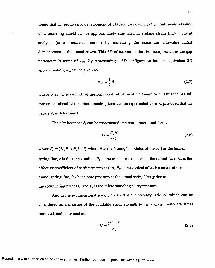
found that the progressive development o f 3D face loss owing to the continuous advance
o f a tunneling shield can be approximately simulated in a-plane strain finite element
analysis (at a transverse section) by increasing the maximum allowable radial
displacement at the tunnel crown. This 3D effect can be then be incorporated in the gap
parameter in terms o f u$D. By representing a 3D configuration into an equivalent 2D
approximation, Mj^can be given by
movement ahead o f the microtunneling face can be represented by u^o, provided that the
values 5x is determined.
The displacement Sx can be represented in a non-dimensional form:
where PQ = (K 0PV + Pv) - P t where E is the Young’s modulus o f the soil at the tunnel
spring line, r is the tunnel radius, P0 is the total stress removal at the tunnel face, K0 is the
effective coefficient o f earth pressure at rest, Pv is the vertical effective stress at the
tunnel spring line, Pw is the pore pressure at the tunnel spring line (prior to
microtunneling process), and Pt- is the microtunneling slurry pressure.
Another non-dimensional parameter used is the stability ratio iV, which can be
considered as a measure o f the available shear strength to the average boundary stress
removed, and is defined as:
(2.5)
where Sx is the magnitude of uniform axial intrusion at the tunnel face. Thus the 3D soil
(2.6)
(2.7)
permission of the copyright owner. Further reproduction prohibited without permission.

13
where cu is the undrained shear strength, H is the depth o f pipe spring line and y is the
soil density.
o 1 2 3 4 5 6 N
o.o 0 .0
1.0 1.01 .1 2
2 .02 .0
3 .03 .0
4 . 04 . 0
5 . 05 . 0
H/D - 4 . 5
H/D - 1 . 5
UNDRAINED CONDITION
H/D - 4 . 5
H/D - 1 . 5
aFigure 2.3 Dimensionless Axial Displacement Q. (After Lee, 1992)
Based on the result o f 3D elastoplastic finite element analyses, the development o f axial
displacement ahead o f the tunnel face (in terms o f the dimensionless parameter Q) with
stability ratio N is shown in Figure 2.3 for H/D o f 1.5 and 4.5. Two soil profiles were
considered: (1) the undrained modulus and shear strength (Eu, cu) are assumed to be
constant with depth; and (2) the undrained strength is assumed to increase linearly with
depth. The elastic modulus is assumed to be proportional to the undrained strength. In
both cases, the vertical initial stresses increase linearly with depth because o f the weight
o f the overburden. As shown in Figure 2.3 (for the case o f K0 = 1), the behavior o f axial
displacement Sx is quite insensitive to the tunnel depth (H/D) or the distribution of soil
properties. For stability ratio N less than about 2.5, a constant dimensionless
Reproduced with permission of the copyright owner. Further reproduction prohibited without permission.

14
displacement O o f 1.12 is obtained for all the variables considered, and the soil mass
ahead o f the face remains largely elastic. It may be seen that deformation increases
rapidly as N exceeds a value o f about 3. This increase in displacement is due to an
increase in the extent o f the plastic zone.
N
o.oUNDRAINED CONDITION
H/D = 1 .51.0
2 .0 - 1.4- 1 . 0
3.0
4.0
5.0
Figure 2.4 Dimensionless Axial Displacement Ahead of the Microtunneling Face with Various K0 Conditions, (after Lee, 1992)
The effect o f K0 ’ not equal to unity is shown in Figure 2.4 for the case o f KQ ’ o f
0.6, 1.0, and 1.4. The results shown in Figure 2.4 are plotted in terms o f £2 as defined by
Equation 2.6. It is found that the dimensionless displacement (Q) is quite insensitive to
various K0'. Equation 2.6 can be used to estimate the equivalent soil movement at the
crown (U3D) due to 3D movements ahead o f the face. The parameter 5X can be determined
Reproduced with permission of the copyright owner. Further reproduction prohibited without permission.

by estimating the non-dimensional displacement Q from Figure 2.3 for a given stability
ratio N and back-calculating 8X from the Equation 2.6. -
2.2.2 Ground Loss Over
The loss o f ground that occurs over the shield corresponds to the volume of soil
that is excavated in excess o f the diameter o f the cutting shield. Causes o f such loss in
microtunneling machine. One o f the common alignment problems is due to the fact that it
is a common practice for the tunnel operator to advance the shield at a slightly upward
pitch relative to the actual design grade thereby avoiding the diving tendency o f the
shield. This excessive pitch will cause overexcavation of the ground near the crown of
the microtunneling machine. The volume o f ground loss (VSh,eid) over the microtunneling
machine can be estimated as:
where R is the microtunneling machine radius, L is the length o f the steerable portion o f
microtunneling machine, and 0 is the excess pitch. An equivalent amount o f ground loss
at the transverse section in terms o f the workmanship parameter w can be obtained by
equating Vshieid with the volume as defined in Figure 2.2:
the Shield
ground are primarily due to alignment problems encountered when steering the
shield (2.9)
where r is the radius o f microtunneling machine.Ignoring the secondary term,
w = Ly.9 (2.10a)
permission of the copyright owner. Further reproduction prohibited without permission.

This equation can be used as a guide to estimate the possible value o f
workmanship parameter w.
Additional ground loss can arise due to the irregular upward or downward
pitching motion o f the shield at an inclination other than the microtunneling design grade.
Ground loss in a similar way occurs owing to yawing, when the microtunneling machine
is allowed to move irregularly from side to side. The occurrence of the irregular motion is
generally intermittent and highly dependent on experience o f the workman controlling
the advance o f the shield. This irregular motion will cause the shield to over-excavate
additional material. This over-excavation problem is primarily related to workmanship
and cannot be precisely determined prior to construction.
2.2.3 Ground Loss Due to the Tail Void
The ground loss, which occurs from the tail void, results because the diameter of
the pipes behind the microtunneling machine is usually less than the diameter of
microtunneling machine. As the microtunneling machine moves forward, the change in
stress state induced in the ground by the excavation causes the ground to squeeze into the
void. This source o f lost ground is represented by the physical gap Gp which is:
Gp = 2At (2.10)
where Af = D — d , D is the outer diameter o f the microtunneling machine, and d is outer
diameter o f the pipe.
Once the soil comes in contact with the pipe, the lining will deflect under the
applied loading. It has been observed that the crown o f the pipe usually will compress
under this loading, whereas the springline will expand [Ward, 1969; Peck et al., 1972].
permission of the copyright owner. Further reproduction prohibited without permission.

However, for most cases, the magnitude o f this component will not be as significant as
the other sources described.
2.3 Ground Movement Due to Concentrated Ground Loss
All the solutions described in the above approach refer to deep problems, i.e; to
cases in which the effect o f the ground surface can be neglected. The purpose of next
approach is to use a ‘strain approach’ for the analysis o f the strains in an incompressible
soil caused by ground losses at moderate depth below the ground surface.
It is well known in continuum mechanics that a free surface adds additional
complexity to a problem. If the irrotationality and the stress-free condition are imposed at
the surface, it leads to trivial solutions, except for perfect (invisicid) fluids. Therefore, a
different approach is needed. The method presented herein tries to solve the problem by
combining the fluid approach with elastic solutions, taking advantage o f their relative
merits. In the first step, the continuum mechanics approach is used, taking the absolute
displacements instead o f velocities as variables. The analysis o f a problem such as that
depicted in Figure 2.5 involves several steps, as listed follows [Sagaseta, 1988].
(a) The effect o f the soil surface is neglected and the strains are computed as though
the ground loss was in an infinite medium (stepl);
(b) These strains will produce some stresses at the top surface, thus violating the
stress-free condition. These stresses can be partially cancelled by one o f the
following methods:
with permission of the copyright owner. Further reproduction prohibited without permission.

18
(i) Considering a virtual source, a negative mirror image o f the actual sink
with respect to the top surface w ill produce opposite normal stresses and
the same shear stresses as the actual sink.
(ii) As in (i), but taking a positive image (i.e., as image sink) will produce the
same normal stresses and opposite shear stresses.
In any case, the strains due to the image are added to those calculated in step 1
(step 2); and
(c) The remaining shear or normal stresses at the surface are then evaluated and
subsequently removed. The resulting strains are again added to those obtained in
steps 1 and 2 (step 3).
Actual ProblemSurface a = 0
t = 0©**
Stepl - Infinite mediumSurface(lngnored) a = <y0
© sink
Step 2 - Image sink/Source(a) Negative image (b) Positive image
© Image source © Image sinkSurfaceOngnored) cr = -cso Surface(lngnored) ____________ a = uq
sink T = To ^ sink * = " r o© Q
Step - 3 Surface stresses(a) | (b)
! -2x0 ii-2<Jo
d> ** d>i i
Sohrfion = s te p l + (step2[a) + step3(a)) or Solution = s te p l + (step2(bj + step3(b)j
Figure 2.5 Steps in Analysis
Steps 1 and 2 involve no consideration o f soil stresses. The stresses at the soil surface
are not evaluated. Instead, the procedure takes advantage o f the fact that the sink and its
image will produce zero shear or normal stresses at their plane of symmetry. However,
Reproduced with permission of the copyright owner. Further reproduction prohibited without permission.
step 3 does require the evaluation o f surface shear or normal stresses which are doubled
by the image sink. Therefore, steps 1 and 2 mean an actual ‘direct strain analysis’ while
step 3 implies the introduction o f stresses and hence the adoption o f a particular soil
model.
O f the two possibilities in step 2, the first is more useful. This arises from the fact
that surface shear stresses will produce displacements in a dominant horizontal direction,
while surface normal stresses will cause greater vertical movement. So, the use o f the
first method provides the possibility o f omitting step 3 o f the analysis, with no stress
evaluation, giving a reasonably accurate solution for the vertical movements which are
generally o f a greater concern than the horizontal movements. This point will be
discussed later, and the relative merits o f both methods will be further analyzed.
If the free-surface condition is to be completely taken in account, then step 3 is
necessary to eliminate the effect o f the surface stresses implied by steps 1 and 2. To
accomplish this, the applied methods derived from the continuum mechanics approach is
needed using the method and techniques of soil mechanics. The following procedure can
be used for step 3:
(a) Evaluate the strains at the surface by differentiation of the displacement field
obtained in steps 1 and 2 (step 3.1);
(b) From these strains, calculate the corresponding surface stresses (step 3.2); and
(c) Obtain the strain field in a half-space subjected to a system of forces acting on its
surface equal and opposite to those calculated in step 3.2 (step 3.3).
The first step is straightforward because the equations arising from the sink in an
infinite medium are simple, as will be shown later. Step 3.2 is also easy, even for a
permission of the copyright owner. Further reproduction prohibited without permission.

relatively complex soil model, because it is used in a direct way for the evaluation of the
stresses from a known strain field. However, step 3.3 is only possible for the simplest
model, i.e., a homogeneous isotropic linear elastic half-space, unless a numerical method
is used.
The assumption o f linear elasticity in step 3.2 is fully justified because the soil
elements at the top surface are generally well away from the sink, and so their plastic
strains will be negligible. The accuracy o f this assumption is not so clear for step 3.3, but
in any case, the difference with respect to a better soil model must be small. The
movements associated with step 3 are small compared with those resulting from steps 1
and 2, particularly if method (i) (negative image sink) is used for the reasons given
earlier.
The basic case considered is the action of a point sink that extracts a finite volume
o f soil at some depth H below the top surface. The extracted soil has a volume V if the
case is in three dimensions, or if a volume per unit length / is in plane strain. For
convenience, in both cases, the amount o f ground loss is defined by the radius a of the
equivalent sphere or cylinder. The analysis is carried out in steps as shown earlier.
2.3.1 Infinite Medium
I f the topsoil is ignored, the problem is symmetric about the sink, and so the
displacement o f any point is only radial, the other components being zero. The condition
o f no volume change implies that the points located at a distance r from the sink must
have an inward radial displacement (Figure 2.6).
(2.11)
permission of the copyright owner. Further reproduction prohibited without permission.

21
where n—2 in plane strain, «=3 in three dimensions, and mi represents the ground loss
v o lum e over a unit length. Equation 2.11 has been derived on the basis o f assumption of
small displacements, neglecting the change in geometry. This assumption will be kept in
the following. For large strains, the equivalent to Equation 2.11 would be
Sr(r0) = r0 - ( r ; - a n)u« (2.12a)
where r is the undeformed (material) co-ordinate for a Lagrangian formulation, or
Sr(r )= {rn + a n)Un - r (2.12b)
where r is the deformed (spatial) co-ordinate for an Eulerian formulation.
Volume Vi
Volume V,
Figure 2.6 Point Sink: Infinite Medium
In a Cartesian reference frame, the displacement components at a point P(x,y,z), if
the sink is at C(x0,y0,z0) (Figure 2.6), are:
in three dimensions and
in plane strain
(2.13a)n r
S (2.13b)n r
S = 0 (2.13c)
Reproduced with permission of the copyright owner. Further reproduction prohibited without permission.

22
n n z — Zs . 2. (2.13d)n r n
where
r = [(x-Jtr<>)2 +C K -y0) 2 + ( ^ ~ Z0)2]I/2
in three dimensions and
r = i ( x - x 0)2 + ( z - z 0)2]1'2
in plane strain.
Surface (Z= 0)
Y Sink
Figure 2.7 Point Sink: Cartesian Co-ordinates
2.3.2 Image Sink: Paved Half-Space
The displacements in Equation 2.12 will produce a certain stress field, depending
on the soil stress-strain properties. At the top surface, normal and shear stresses will
result so violating the imposed boundary condition o f a free surface.
These surface stresses can be partially removed by the use o f image sinks or
sources as described in the preceding section. I f a negative image is used, then the surface
normal stresses are eliminated, while a positive image will cancel the shear stresses.
Following the first possibility (method (ii)), the result is a half-space whose top
surface has no normal vertical stress but is totally constrained in the horizontal direction.
The situation is as though the soil surface was covered by a flexible but not extensible
membrane. This situation will be referred to by the term ‘paved’ half-space.
Reproduced with permission of the copyright owner. Further reproduction prohibited without permission.

This condition is not too far from reality. A relatively stiff pavement is common
above underground utility in urban areas. Where soil movements caused by nearby
excavations are o f interest. It is common practice when surface movements are measured
in urban areas to refer the observation points to a given depth to avoid the influence of
the pavement. Under these conditions, the paved solution may be at least as good as the
assumption o f a completely free surface. This consideration is especially valid for the
vertical component o f the displacement.
Figure 2.8 Point Sink-Negative Image: (a) Three Dimensions and (b)TwoDimensions
Adding the displacements caused by the sink and its negative image, the
following result is obtained for the points on the plane XZ (other points are defined either
by the plane strain or the axial symmetry condition) (Figure 2.8):
,P(X.OJZi
(O.O.hJ(O.O.ft)
Axial symmetry
Z
(2.14a)
S = 0y (2.14b)
permission of the copyright owner. Further reproduction prohibited without permission.

Where
rI = [x 2 + (z -A )2],/a
rz =[x2 +(z + h)2]'/2
I f a positive image were to be used (method (ii)), the result would be a half-space
whose surface is free in the horizontal direction but which can not undergo any vertical
movement as though it were suspended from a system of inextensible wires. This
condition is completely unrealistic. The only reason for keeping this method in mind is
that it will be used in a later stage as a tool for theoretical reasoning regarding the
movements of the top surface.
2.3.3 Free Surface
For the complete elimination of the surface stresses, the procedure described
earlier must follow steps 3.1-3.3.
8SX dS hx „ .(2 -15)
For a linear elastic material, the associated shear stresses are (step 3.2)
hx (x 2+ h 2)'
r = G r = -4G a\ 2 , ^ (2.16)
The shear stress distribution is shown in Figure 2.9, for both the plane strain and
plane stress cases.
Reproduced with permission of the copyright owner. Further reproduction prohibited without permission.

25
jev4 i
o.
o.
o.
-2- 0.1
- 0.2
-0.3
4 6 8 10
-0.4 JFigure 2.9 Point Sink: Surface Shear Stresses
Step 3.3 o f the analysis involves the evaluation o f the displacement in a
homogeneous linear elastic half-space subjected to a system o f horizontal forces at its
surface acting oppositely to the shear stresses (Equation 2.16). This can be performed by
direct integration o f the known solution for a horizontal point load. The results, for the
plane strain case, are:
(2.17a)
(2.17b)
where
r2 = [x2 + (z + /2)2r 2
In the three dimensional case.
x[TEE (k) + I FF(k)]dcc
Reproduced with permission of the copyright owner. Further reproduction prohibited without permission.

26
5 . = - a 2hz f “ — x [ J EE (k) + F (k)]da (2.18b)‘r k Jo rb Qi +a~)
where
/£=i+±z2(-V+4 )2 r. rh
I F = - ( a z + x 2 -t-2z2)
a (a — x)J E = - 1 + 2-
ra = K a - x y - + z 2]U2
r6 = [ (a + x)2 + z 2]l/2
F(k) and E(k) are complete elliptic functions o f the first and second kind respectively,
with
* = a - 4 )r a \ 1 /2
rb
The integrals o f Equation 2.18 must be evaluated numerically.
2.3.4 Surface Movements
The addition o f the displacement in Equations 2.17 or 2.18 to the values in
Equation 2.14 defines the final value o f the soil movements at any point. In most cases,
attention is mainly focused on the displacements o f the soil surface. Determination of
stresses (step 3 o f the general procedure) is not necessary.
The simplicity comes from the fact that, for an incompressible material (Poisson’s
ratio o f 0.5), the application o f a vertical point load at the soil surface produces zero
Reproduced with permission of the copyright owner. Further reproduction prohibited without permission.

27
horizontal movements at surface points, and the surface vertical displacement due to a
horizontal load are also zero [Sagaseta,1988].
With this in mind, i f the vertical movements are considered, the superposition of
the negative image will cancel the surface normal stresses and the relief o f the remaining
surface shear stresses will not mean any additional vertical movement, and hence it can
be omitted.
To obtain the horizontal surface displacement, the alternative possibility o f
method (ii) can be followed. In this case, the surface shear stresses will be cancelled, and
then subsequent removal o f the remaining normal stresses will produce no additional
horizontal movement and so can be avoided.
As the vertical movements o f the soil surface are doubled by the negative image
and the horizontal displacements are also doubled by the positive image, the conclusion is
that the surface movements can be directly obtained simply by multiplying the
movements due to the sink in an infinite medium by a factor of 2 ignoring the presence o f
the soil surface.
In this way, the final exact displacements o f the soil surface due to the point sink
are:
s ' ° = = _ 2 T ( x ! + a j ) " ! ( 2 l 9 a )
( 2 1 9 b )
where h is the depth of the tunnel spring line. For two dimenal case, these values are
shown in Figure 2.10. In Figure 2.10 the unit o f y axis is S/a2, the unit o f x axis is x/h.
Reproduced with permission of the copyright owner. Further reproduction prohibited without permission.

28
S 0.6IB
CO0.4
0.2
x/h10
- 0.2
HorizontalV e r t ic a l
-0.4
- 0.6
- 0.8
-1 .2 : J
Figure 2.10 Point Sink: Final Surface Displacement
2.4 Ground Movement Associated with Microtunneling
The equivaJent ground loss parameter obtained in Equation 2.4 can be further
modified to incorporate the non-uniform radial movement o f the soil (due to the oval
shaped gap) around the tunnel, which basically influences the deformation pattern o f the
surrounding soil. The component o f the equivalent ground loss parameter sXvZ=o which
causeS the surface settlement may be derived by adopting an exponential function to the
equivalent ground loss parameter so that models the non-uniform movement o f the soil
around the tunneling as shown in Figure 2.11.
£x,~o=£oBe-Ax2 (2-20)
where A, B are constants, and So = equivalent ground loss and is defined as:
Reproduced with permission of the copyright owner. Further reproduction prohibited without permission.

2 9
x 100% = 4 g r \ g x 100% nr~ 4r~
Constants g is gap parameter, r is radius o f microtunneling face, A and B are derived
based on the boundary conditions described next.
When the portion o f the soil above the tunnel crown touches the tunnel lining, the
soil at the side o f the tunnel displaces towards the bottom o f the tunnel. Therefore, the
upward movement o f soil below the tunnel is limited. Centrifuge model tests carried out
by Stallebrass et al. [1996] revealed similar results. When the tunnel lining settles on the
bottom o f the annulus gap (due to the self-weight), the distance between the crown o f the
tunnel lining and crown o f the excavated surface becomes twice the thickness o f the
annulus gap. Based on simple geometry, the void area above the tunnel spring line is
about 75% o f the total void area. Therefore, 75% percent o f vertical ground movement
occurs within the upper annulus o f the gap around the tunnel. Figure 2.11 shows the
vertical ground movement influence zone where most o f the soil displacements occur.
The relationship between settlement trough width, which is an indirect measure o f the
ground movement influence zone, and the tunnel depth can be expressed as a horizontal
angle /?, drawn from the spring line o f the tunnel to the width o f the settlement trough at
the surface. From the observations made by Cording and Hansmire [1975], the P value is
about 45° for soft to stiff clays. The ground movement occurs predominantly within the
45° wedge in between the ground surface and the tunnel. Therefore, it may be considered
that the surface settlement above the tunnel axis is the resultant o f the complete
cumulative equivalent ground loss (100%eo) around the tunnel, and the surface settlement
Reproduced with permission of the copyright owner. Further reproduction prohibited without permission.

at a horizontal distance (h+r) is the resultant o f partial cumulative equivalent ground loss
(25%s0). These boundary conditions are shown in Figure 2.11 (Loganathan 1998).
Ground surface
Assured wedge boudary y
Actual ground loss zxz
Pipe Average ground
Figure 2.11 Ground Deformation Pattern and Ground Loss Boundary Conditions
By applying these boundary conditions, the equivalent ground loss component
those models the nonuniform vertical movement is derived as:
— 1.38x2eQ exp (2 .21)L (a +'O2
Observation made by Deane and Bassett [1995] and Tallebrass et al. [1996] show
that the horizontal ground movement into the tail void or gap is at a maximum at the
spring line o f the tunnel and is zero at the crown and the invert o f the tunnel. Therefore,
the lateral ground movement is symmetrical about the tunnel axis. The lateral movement
component is incorporated into the ground loss as shown:
(2.22)
where C and D are constants that are derived based on the boundary conditions.
Reproduced with permission of the copyright owner. Further reproduction prohibited without permission.

31
Based on the oval-shaped gap geometry, the magnitude o f the horizontal movement at the
tunnel spring line is approximately half o f the vertical movement at the tunnel crown,
which causes 75% of the ground movement into the upper annulus o f the oval-shaped gap
around the tunnel. Therefore, the equivalent ground loss component due to the horizontal
movement at horizontal distance x and depth h is 50% o f the equivalent ground loss
causing surface settlement at horizontal distance x. By applying these boundary
conditions and substituting Equation 2.21 in Equation 2.22, the modified equivalent
ground loss parameter, incorporating the nonlinear ground movement around the tunnel
soil interface, may be defined as
4gr + g 2 4 r 2= - - 7.2 - exP ~
1.38.x2 0.69z2^ (2.23)Xh + r)2 h 2
where h is the depth o f the pipe, r is the radius of pipe, and g is gap parameter.
Substituting Equation 2.23 in Equation 2.19, we get:
Sx = - - - •■■ * . (2.24a)7t ( x + h )
S t = ^ , k , (2.24b)K (x2 +/ l2)
and the ground movement at the surface can be defined by:
s - s _ 4gr + g 2 f 1.38x2— ^ x (.z= 0 ) ~~ 4 y 2 (h + r) ^•(x2 + h2)
(2.25a)
4gr-*-g2 ( 1.38x2 ̂ h „4r2 eXP[ (h + r f j x t f + h ' ) ( ’
The Sz value is shown in Figure 2.12. Figure 2.12 shows that the deeper microtunneling
is the wider the trough is and smaller the maximum ground settlement is
Reproduced with permission of the copyright owner. Further reproduction prohibited without permission.

Gro
und
Settl
emen
t (S
)
3 2
0.02
-16 2D1812
- 0.02
-0.04
-0.06
-0.08
h = r h = 2x h =4x h = 10x
- 0.12
-0.14
-0.16
-0.18
Distance from Centerline (x)Figure 2.12 Vertical Ground Movement
Reproduced with permission of the copyright owner. Further reproduction prohibited without permission.

CHAPTER 3
EMPIRICAL APPROACH
A quite extensive survey o f tunnel-induced (large diameter) ground movements
has been compiled and tabulated [Attewell, 1989]. The settlement caused by tunnels in
granular soils shows considerable scatter in a significant number o f cases. Settlement
often is greater than 100mm. The majority o f tunnels in cohesive soils show settlements
below 50 mm, and further investigation has shown that these settlements can be foreseen
quite reliably in most cases.
Figure 3.1 Surface Settlement Trough
The free ground settlement w has been conveniently approximated by normal and
cumulative probability functions as:
X
z
y
(3.1)
33
Reproduced with permission of the copyright owner. Further reproduction prohibited without permission.

3 4
where Vs is the soil-loss-induced surface settlement volume per meter of tunneling
machine advance, i is a parameter which is equivalent to the standard deviation o f a
statistical normal distribution, x,y are the ground coordinates along and transverse to the
tunnel center line respectively, is the tunnel starting point, and xy is the microtunneling
machine face position.
For a position remote from the start, and at a distance o f at least three times the
tunnel depth behind the microtunneling machine face, the transverse soil-loss-induced
surface settlement profile can be defined by:
and the center maximum settlement is:
In the above two equations, the s subscript is used to denote short-term (i.e., from ground
loss rather than long-term consolidation). The surface settlement volume is appropriately
double-subscripted.
Settlement volume Vss can be estimated from the proposed tunneling rate and
method, deduced rate o f soil relaxation [Attewell, 1978], or by the choice o f an
appropriate percentage o f face area base on similar tunneling case histories, usually in the
range 0.5% to 2.5% o f the face area for clay soils. O’Reilly and New [1982] have
proposed the empirical expressions for evaluation o f the parameter is for U.K. conditions
as:
(3.2)
is = 0.43(z0 — z) +1 Am for clay soil (3<zo<34m) (3.4)
Reproduced with permission of the copyright owner. Further reproduction prohibited without permission.

Gro
und
S»t
tl«m
»nt
35
when consolidation effects are significant In the above equations, zo is the tunnel axis
depth, and z is depth to the settlement reference surface (zero for surface).
In addition to an increased maximum settlement, the width o f the zone of
influence may also be increased by the consolidation mechanism. It has been proposed by
Hurrell [1985] that the long-term transverse settlement profile comprises the
superposition o f the short-term settlement and o f two discrete consolidation settlement
profiles. The long-term profile is then defined as:
"V = “W , + “W (e x p [~ (y 4;g ) 2 ] + exPr fa,~J>)‘» (3-5)21; 21] 2is
where wc is the consolidation element o f transverse settlement. As shoen in Figure 3.12,
this is a relatively smooth profile, but not necessarily a pure normal probability curve. In
practice, however, a curve close to this is obtained.
1.5-1.5
-w* W cL eft• W c Right
W total
Distance from Centerline
Figure 3.2 Short-Term and Long-Term (Consolidation) Settlements at GroundSurface
Use of empirical Equation 3.5 can be reasonably justified in ground having
permeability isotropy. However, there are examples in the U.K. o f long-term settlement
measurements in which the character o f the ultimate settlement trough cannot be satisfied
by this equation. Non-compliance may be attributed to several factors, and particularly to
Reproduced with permission of the copyright owner. Further reproduction prohibited without permission.

36
a state o f ground permeability anisotropy. Take, for example, the case o f stratified ground
in which the horizontal permeability kh is greater than the vertical permeability kv_ Then,
following flow net procedure, the scaling factor is:
KVk (3.6)
After Hurrell [1987], let the potential spread o f the long-term transverse settlement
trough, y t be:
y ,= 2 S z 0 (3.7)
In the case o f anisotropic permeability, the standard deviation it(a) for the long-term
surface settlement trough is estimated as:
i« » = y ‘A (3-8)
Thus, Equation (3.5) may be generalized for both anisotropic permeability and long-term
settlement:
(3 -9)V2 jn,w
Definition o f the complete form o f the long-term transverse settlement trough is then:
M .y)t — wmaxf exp[- y 112zf2] — permeability isotropy (3.10)
M y), = Wrmxr exPl~ y Z/ 2if{a) 1 ~ permeability anisotropy (3.11)
There were two microtunneling experiment carried out at Waterways Experiment
Station (WES) in Vicksburg, MS [Bennett, 1993; Bennett, 1997]. The micro tunneling
demonstrations and evaluations were performed during 1992, and 1995 at a specially
constructed test facility built at WES [Bennett, 1993]. Some o f the results and calculated
Reproduced with permission of the copyright owner. Further reproduction prohibited without permission.

37
ground settlement o f these two experiments are listed and compared with numerical
method and neural network method in this dissertaion. -
Reproduced with permission of the copyright owner. Further reproduction prohibited without permission.
CHAPTER 4
NUMERICAL APPROACH
4.1 FLAC3P Software
Flac3D is an explicit finite difference program for numerical study o f the
mechanical behavior o f a continuous three-dimensional medium as it reaches equilibrium
or steady-state flow. Materials are represented by polyhedral elements within a three-
dimensional grid adjusted by the user to fit the shape o f the object to be modeled. Each
element behaves according to a prescribed linear or non-linear stress/strain law in
response to applied forces or boundary restraints. The material can yield and flow, and
the grid can deform (in Iarge-strain mode) and move with the material represented.
Flac3D offers a wide range o f capabilities to solve complex problems in mechanics
and especially in geomechanics. The Flac3D version 2.0 has ten built-in material models:
1. null;
2 elastic, isotropic;
3. elastic, orthotropic;
4. elastic, transversely isotropic;
5. Drucker-Prager plasticity;
6 . Mohr-Coulomb plasticity;
7. strain-hardening/softening Mohr-Coulomb plasticity;
8 . ubiquitous-joint plasticity;
38
Reproduced with permission of the copyright owner. Further reproduction prohibited without permission.

39
9. bilinear stxain-hardening/softening ubiquitous-joint plasticity; and
10 . modified cam-clay plasticity.
Each model is developed to represent a specific type o f constitutive behavior
commonly associated with geologic materials. The null model is used to represent
material that is removed from the model but with the associated zones left in place. The
elastic, isotropic model is valid for homogeneous, isotropic, continuous materials that
exhibit linear stress-strain behavior. The elastic, orthotropic model and the elastic,
transversely isotropic model are appropriate for elastic materials that exhibit well-defined
elastic anisotropy. The Drucker-Prager plasticity model is a simple failure criterion in
which the shear yield stress is a function o f isotropic stress. The Mohr-Coulomb plasticity
model is used for materials that yield when subjected to shear loading, but the yield stress
depends on the major and minor principal stresses only; the intermediate principal stress
has no effect on yield. The strain-softening Mohr-Coulomb model is based upon the
Mohr-Coulomb model, but is appropriate for materials that show degradation or increase
in shear strength when loaded beyond the initial failure limit. The ubiquitous-joint model
applies for a Mohr-Coulomb material that exhibits a well-defined strength anisotropy.
The bilinear strain-softening ubiquitous-joint model combines the strain-softening Mohr-
Coulomb model with the ubiquitous-joint model. This model includes a bilinear failure
envelope for both the matrix and the ubiquitous joints. The modified Cam-clay model
accounts for the influence o f volume change on deformability and on resistance to failure.
Reproduced with permission of the copyright owner. Further reproduction prohibited without permission.

40
Table 4.1 FLAC3D Constitutive Models i[after FLAC3D Menu)Model Representative Material Example Application
nullvoid holes, excavations, regions in
which material will be added at later stage
elastichomogeneous, isotropic continuum;linear stress- strain behavior
manufactured materials (e.g., steel) loaded below strength limit; factor-of-safety calculation
orthotropic elasticelastic materials with three mutually perpendicular axis o f elastic symmetry
columar basalt loaded below strength limit
transversely isotropic elastic
thinly laminated material exhibiting elastic anisotropy (e.g., slate)
laminated material loaded below strength limit
Drucker-Pragerplasticity
limited application; soft clays with low friction
common model for comparison to implicit finite-element programs
Mohr-Coulombplasticity
loose and cemented granular materials; soils, rock, concrete
general soil or rock mechanics (e.g. slope stability and underground excavation)
strain-hardening / softening Mohr- Couloomb
granular materials that exhibit non-linear material hardening or softening
studies in post-failure (e.g., progressive collapse, yielding pillar, caving)
unbiquitous-jointthinly laminated material exhibiting strength anisotropy (e.g., slate)
excavation in closely bedded strata
bilinear strain- hardening / softening ubiquitous-joint
laminated materials that exhibit non-linear material hardening or softening
studies in post-failure o f laminated materials
modified Cam-Clay
materials for which deformability and shear strength are a function o f volume change
geotechnical construction on clay
In addition, three optional features are available in Flac3D for dynamic analysis,
thermal analysis, and modeling creep material behavior:
1. The dynamic analysis option permits three-dimensional, fully dynamic analysis. The
calculation is based on the explicit finite difference scheme to solve the full equations
o f motion. The dynamic option extends Flac3D’s analysis capability to a wide range
Reproduced with permission of the copyright owner. Further reproduction prohibited without permission.

41
o f dynamic problems in disciplines such as earthquake engineering, seismology, and
mine rockbursts.
2. The thermal analysis option allows simulation o f transient heat conduction in
materials and the subsequent development of thermally induced stresses.
3. The creep analysis option can be used to simulate the behavior of materials that
exhibit creep, i.e., time-dependent material behavior. There are five creep models in
this option: the classical viscoelastic (Maxwell) model, a two-component power law,
a reference creep formulation implemented for nuclear waste isolation studies, a
viscoplastic model that combines the reference creep formulation with the Drucker-
Prager plasticity model, and a “crushed-salt” model that simulates both volumetric
and deviatoric creep compaction.
FIac3D also contains a powerful built-in programming language, FISH, which
enables the user to define new variables and functions. FISH offers a unique capability to
users who wish to tailor analyses to suit their specific needs.
4.2 Basic Definitions of Flac3P Terms (after FlacJL> Menu)
FIac3D Model — The Flac3D model is created by the user to simulate a physical problem.
When referring to a FIac3D model, the model implies a sequence of Flac3D commands
that define the problem conditions for numerical solution.
Zone — The finite difference zone is the smallest geometric domain within which the
change in a phenomenon (e.g., stress versus strain) is evaluated. Polyhedral zones of
different shapes (e.g., brick, wedge, pyramid, and tetrahedral shaped zones) are used to
create models.
Reproduced with permission of the copyright owner. Further reproduction prohibited without permission.

4 2
Gridpoint — Gridpoints are associated with the comers o f the finite difference zones.
There are five, six, seven, or eight gridpoints associated with each polyhedral zone,
depending on the zone shape.
Finite Difference Grid — The finite difference grid is an assemblage of one or more
finite difference zones across the physical region being analyzed.
Boundary Conditions — A boundary condition is the prescription o f a constraint or
controlled condition along a model boundary.
Constitutive Model — The constitutive model represents the deformation and strength
behavior prescribed to the zones in a Flac3D model.
Step — Because Flac3D is an explicit code, the solution to a problem requires a number o f
computational steps. During computational stepping, the information associated with the
phenomenon under investigation is propagated across the zones in the finite difference
grid. A certain number o f steps are required to arrive at an equilibrium state for a static
solution. When using the dynamic analysis option, Step refers to the actual time step for
the dynamic problem.
Unbalanced Force — The unbalanced force indicates when a mechanical equilibrium
state (or the onset o f plastic flow) is reached for a static analysis. The maximum
unbalanced force will never exactly reach zero for a numerical analysis. The model is
considered to be in equilibrium when the maximum unbalanced force is small compared
with the total applied forces in the problem.
Large Strain/Small Strain — By default, Flac3D operates in small-strain mode; that is,
gridpoint coordinates are not changed even if computed displacements are large. In the
Reproduced with permission of the copyright owner. Further reproduction prohibited without permission.
43
large-strain mode, gridpoint coordinates are updated at each step according to computed
displacements. In the large-strain mode, geometric nonlinearity is possible.
4.3 Intrinsic Deformability Properties
All material models in FLAC,3D except for the transversely isotropic elastic and
orthotropic elastic models, assume an isotropic material behavior in the elastic range
described by two elastic constants, bulk modulus (K) and shear modulus (G). The elastic
constants, K and G, are used in FLAC rather than Young’s modulus, E, and Poisson’s
ratio, v, because it is believed that bulk and shear moduli correspond to more fundamental
aspects o f material behavior than do Young’s modulus and Poisson’s ratio. The equations
to convert from (E, v) to (K, G) are:
K = ---- - ---- (4.1)3(1-2 v )
G = — —— (4.2)2(1 + v)
Equation 4.1 should not be used blindly when v is near 0.5 since the computed value o f K
will be unrealistically high and convergence to the solution will be very slow. It is better
to fix the value o f K at its known physical value (estimated from an isotropic
compression test or from the P-wave speed), and then compute G from K and v.
The basic criterion for material failure in FLAC3D is the Mohr-Coulomb relation,
which is a linear failure surface corresponding to shear failure:
/ , = cr, - <x3 AT, + 2 cJ n ; (4.3)
where N$ = ( 1+ sin<j>)/(l-sin<{>),
07 = major principal stress,
o j = minor principal stress,
Reproduced with permission of the copyright owner. Further reproduction prohibited without permission.

4 4
<p = friction angle, and
c = cohesion.
Shear yield is detected i f / s < 0. The two strength constants, (f> and c, are conventionally
derived from laboratory triaxial tests.
4.4 Modeling Procedure
For modeling purposes, the problem is defined by the domain sketched in Figure
4 1 where sdvantHge hss been tsksn o f the hslf^symmctry geometry 2nd pisin strnin
condition. A system o f reference axes is selected with the origin located at the
intersection o f the cavity axis with the front face o f the domain and the z-axis pointing
upward. The boundary conditions applied to this domain are
Figure 4.1 Domain for Flac3D Simulation — Half Symmetry
Reproduced with permission of the copyright owner. Further reproduction prohibited without permission.

45
<1
Plane View Side View
Figure 4.2 Boundary Conditions for Flac3D Analysis — Half Symmetry
sketched in Figure 4.2. The displacements o f the x, y, and z direction at far right and
boundary are restricted in all directions.. The displacements o f the symmetry boundary
corresponding to the plane at x = 0 is restricted in the x-direction. Plain strain is assumed
along the y-plane. The thickness of the domain is selected as 4m. The domain is
discretized into one layer o f zones organized in a pattern shown in Figure 4.3.
Figure 4.3 Flac3d Grid — H alf Symmetry
Reproduced with permission of the copyright owner. Further reproduction prohibited without permission.

46
The Flac3D model is initialized by first simulating gravity loading to develop the in-situ
state of stress in the soil. Initial internal stresses that satisfy both equilibrium and
gravitational gradient are applied to the domain. The initialized stresses will cut the
number of time steps taken for the model to reach equilibrium due to gravity. The
displacements o f the soil due to the gravitational forces are then initialized to zero. The
microtunneling machine and following pipe are modeled at a depth from the ground
surface. The soil surrounding the microtunneling machine is assumed to deform under
plane strain conditions. To simulate the microtunneling process, a cavity around the pipe
is created. Then the soil will fall onto the pipe’s outside surface. Once the soil contacts
the pipe surface, the pipe will stop the soil’s further movement. The pipe and soil will
interact until the equilibrium condition is reached. The soil is assumed to be
homogeneous and is assigned a Mohr-Coulomb material model.
4.5 Selection o f Boundary and Zones
Two important points o f concern in building any model are:
1. How the location o f the grid boundaries influence model results; and
2. The density o f zoning required for an accurate solution in the region o f interest
4.5.1 Selection o f Boundary Condition
Artificial boundaries are introduced to enclose the chosen number o f zones. In the
test for selecting an artificial boundary for the semi-infinite soil media as shown in Figure
4.1, the far-right boundary and the far boundary in the negative z-direction were
evaluated. The distance between far boundary global axis (D) is 5 x H to 8 x H. The
Reproduced with permission of the copyright owner. Further reproduction prohibited without permission.

47
vertical soil displacements on the ground surface were compared. Figure 4.4 shows the
location o f the points where the vertical soil displacements are measured.
Figures 4.5, 4.6, 4.7, and 4.8 show the ground settlement trough at D = 5H, D =
6H, D = 7H, and D = 8H respectively. Figure 4.9 shows a comparison o f the result for
surface settlement at point A-F. Table 4.2 shows the comparison in table format. All
ground settlement troughs are similar, but the magnitude of ground settlement increases
with the D to H ratio. The ground settlement at D = 7H is almost same as D = 8H. This
indicates that to simulate the ground settlement associated with microtunneling with
FLAC,3D the far boundary distance equal to seven times the microtunneling machine
depth is sufficient to obtain accurate results.
Ground Surface
H
Far Boundary
Figure 4.4 Model Showing Locations of Ground Surface Points
Reproduced with permission of the copyright owner. Further reproduction prohibited without permission.

48
0_ - 0.001 % - 0.002 I -0 003| -0.004 % -0.005 * -0.006 | -0.007 = -0.008
-0.009
Figure 4.5 Ground Settlement Trough at D = 5H
60 7 010 40- 0.002
-0.004
-0.006
-0.008
- 0.01
- 0.012
Distance from Centerline (m)
Figure 4.6 Ground Settlement Trough at D = 6H
t o
Distance from Centerline (m)
Reproduced with permission of the copyright owner. Further reproduction prohibited without permission.

4 9
0.002
40 80 10060- 0.002
-0.004
-0.006
-0.008
- 0.01
- 0.012
D istance from Centerline (m)
Figure 4.7 Ground Settlement Trough at D = 7H
60 70 8020 , 30 40 50- 0.002
-0.004
-0.006
-0.008
- 0.01
- 0.012
D istance from Centerline (m)
Figure 4.8 Ground Settlement Trough at D = 8H
Reproduced with permission of the copyright owner. Further reproduction prohibited without permission.

5 0
12- 0.002
-0.004
-0.0065H6H7H
-0.008
- 0.01
- 0.012
Distance from Centerline (m)
Figure 4.9 Comparison of Soil Displacement for Different Boundary Conditions
Table 4.2 Vertical Soil Displacements on the Ground Surface
PointsDistance along the horizontal
axis x (m)
Vertical Soil Displacements in mm
5H 6H 7H 8H
A 0.0 -9.33 -9.87 -10.2 -10.2
B 2 -8.99 -9.49 -9.83 -9.83
C 4 -8.08 -8.54 -8.81 -8.80
D 6 -6.90 -7.32 -7.53 -7.50
E 8 -5.73 -6.08 -6.25 -6.22
F 10 -4.64 -4.94 -5.07 -5.04
4.5.2 Selection of Pipe Material
In this test, two different pipe materials were examined, Steel and HDPE (elastic
behavior only). The mechanical property o f A36 Steel and HDPE is listed in Table 4.3.
Reproduced with permission of the copyright owner. Further reproduction prohibited without permission.

51
The pipe is considered using an elastic model in FLAC3D analysis. The result o f ground
movement is shown in Figure 4.10. The shape of the two settlement troughs is very
similar, and the maximum vertical displacement is almost same. This shows that the pipe
properties do not significantly affect the vertical displacement. In the following numerical
analysis, the A36 steel pipe is used.
Table 4.3 Mechanical Property of A36 Steel and HDPEA3 6 Steel HDPE
Elastic Modulus KPa (psi) 2.0x10⁸ (2.90x10⁷) 896x103 n ^nvin5'*V-----------------v /
Tensile Yield Strength Kpa (psi) 248x103 (36000) 22x103 (3200)Compressive Yield Strength Kpa
(psi)248xl03 (36000) l l x lO 3 (1600)
The ground movements were studied in different type o f soils due
microtunneling. The soil parameters were selected from the Flac3D manual. Table 4.4
gives the types o f soils selected and their respective strength properties.
Figure 4.11 shows the graphs for vertical displacement o f soil at the ground
surface for the selected soils. The figure indicates that the ground movement for gravel,
sandy gravel, and sand were smaller compared to the silt and clay soils. The maximum
surface displacement o f soil for silt and clay was higher than the maximum surface
displacement o f soil for gravel and sand. The reason for the movement for gravel and
sand soil being smaller than the movement for clay and silt is that the elastic modulus of
gravel and sand is much higher than the elastic modulus o f silt and clay. However, it
should be noted that sand and gravel are still at risk of significant face stability problems
leading to large ground movements.
Reproduced with permission of the copyright owner. Further reproduction prohibited without permission.

52
20 6040
- 0.002
-0.004SteelHDPE
- 0.01
- 0.012Distance from Center Line of Microtunneling Macchine (m)
Figure 4.10 Vertical Displacement at Ground Surface For Different Pipe Materials
Table 4.4 Selected Elastic Constants and Strength Properties for Soils [Oritz et al.,198 61
Soil Dry Density (kg/mA3)
ElasticModulus
(Mpa)
(Cohesion(Kpa)
Friction Angle (degree)
Gravel 1600 40 34-32Sandy Gravel with few fines 2100 40 35-32Sandy Gravel with silty or Clayey fines
2100 40 1 35-33
Mixture of Gravel and sand with fines
2000 15 3 28-22
Uniform sand - fine 1600 15 32-30Uniform sand — coarse 1600 25 34-30Well-graded sand 1800 20 33-32Low plasticity silt 1750 4 2 28-25Medium to high plasticity silt 1700 3 3 25-22Low plasticity clay 1900 2 6 24-20Medium plasticity clay 1800 1 8 20-10High plasticity clay 1650 0.6 10 17-6Organic silt or clay 1550 0.5 7 20-15
Reproduced with permission of the copyright owner. Further reproduction prohibited without permission.

53
0.002
- 0.002
c 0 E 0 ■ o raC LCO
-0.004
Q -0 .006rootr0> -0 .008
- 0.01
- 0.012
70
Gravel Gravel 2 Gravel 3 Gravel 4 Sand 5 Sand 6 Sand 7
— Silt 8
ClaylOClayl 1Clay 12Clayl 3
80
Distance from Center Line of Microtunneling Machine (m)Figure 4.11 Simulated Ground Movement with Different Soil Type (See Table 4.4
for soil type description)
Reproduced with permission of the copyright owner. Further reproduction prohibited without permission.

Reproduced
with perm
ission of the
copyright ow
ner. Further
reproduction prohibited
without
permission.
Table 4.5 Ground Displacement (meter) for Different Types of SoilDistance Gravel Gravel 2 Gravel 3 Gravel 4 Sand 5 Sand 6 Sand 7 Silt 8 Slit 9 ClaylO Clayl 1 Clay 12 Caly13
0.00E+00 -2.31E-03 -3.20E-03 -3.20E-03 -7.80E-03 -6.43E-03 -3.76E-03 -5.60E-03 -1.08E-02 -1.01E-02 -1.02E-02 -1.03E-02 -9.77E-03 -8.52E-032.00E+00 -2.24E-03 -3.11E-03 -3.11E-03 -7.56E-03 -6.23E-03 -3.66E-03 -5.44E-03 -1.04E-02 -9.76E-03 -9.87E-03 -9.85E-03 -9.36E-03 -8.16E-034.00E+00 -2.08E-03 -2.88E-03 -2.88E-03 -6.92E-03 -5.73E-03 -3.38E-03 -5.02E-03 -9.46E-03 -8.86E-03 -8.95E-03 -8.82E-03 -8.32E-03 -7.27E-036.00E+00 -1.86E-03 -2.58E-03 -2.58E-03 -6.10E-03 -5.08E-03 -3,01 E-03 -4.46E-03 -8.22E-03 -7.71 E-03 -7.76E-03 -7.52E-03 -7.00E-03 -6.14E-038.00E+00 -1.63E-03 -2.26E-03 -2.26E-03 -5.27E-03 -4.40E-03 -2.63E-03 -3.88E-03 -6.99E-03 -6.54E-03 -6.55E-03 -6,21 E-03 -5.68E-03 -4.96E-03
1.00E+01 -1.41E-03 -1.95E-03 -1.95E-03 -4.49E-03 -3.77E-03 -2.26E-03 -3.34E-03 -5.85E-03 -5.46E-03 -5.43E-03 -5.00E-03 -4.47E-03 -3.88E-03
1.19E+01 -1.23E-03 -1.70E-03 -1.70E-03 -3.90E-03 -3.28E-03 -1.97E-03 -2,91 E-03 -4.99E-03 -4.64E-03 -4.58E-03 -4,11 E-03 -3.61 E-03 -3,11 E-03
1.40E+01 -1.06E-03 -1.46E-03 -1.46E-03 -3.33E-03 -2.81 E-03 -1.69E-03 -2.49E-03 -4.19E-03 -3.88E-03 -3.79E-03 -3.29E-03 -2.80E-03 -2,41 E-03
1.63E+01 -8.97E-04 -1.24E-03 -1.24E-03 -2.82E-03 -2.38E-03 -1.43E-03 -2,11 E-03 -3.48E-03 -3.20E-03 -3.08E-03 -2.59E-03 -2.10E-03 -1.80E-031.80E+O1 -7.52E-04 -1.04E-03 -1.04E-03 -2.36E-03 -1.99E-03 -1.20E-03 -1.78E-03 -2.85E-03 -2.60E-03 -2.48E-03 -1.99E-03 -1.54E-03 -1.28E-03
2.15E+01 -6.22E-04 -8.66E-04 -8.66E-04 -1.96E-03 -1.65E-03 -9.95E-04 -1.47E-03 -2.31E-03 -2.09E-03 -1.95E-03 -1.48E-03 -1.07E-03 -8.64E-04
2.46E+01 •5.08E-04 -7.09E-04 -7.09E-04 -1.60E-03 -1.35E-03 -8.13E-04 -1,21 E-03 -1.84E-03 -1.64E-03 -1.51 E-03 -1.07E-03 -6.96E-04 -5.26E-04
2.79E+01 -4.08E-04 -5.71 E-04 -5.71 E-04 -1.29E-03 -1.09E-03 -6.52E-04 -9.70E-04 -1.44E-03 -1.27E-03 -1.14E-03 -7.38E-04 -4.15E-04 -2,61 E-04
3.16E+01 -3.20E-04 -4.50E-04 -4.50E-04 -1.01E-03 -8.54E-04 -5.12E-04 -7.63E-04 -1.11E-03 -9.53E-04 -8.35E-04 -4.65E-04 -1.89E-04 -6.93E-05
3.56E+01 -2.44E-04 -3.45E-04 -3.45E-04 -7.76E-04 -6.52E-04 -3.91E-04 -5.84E-04 -8.19E-04 -6.93E-04 -5.82E-04 -2.64E-04 -3.68E-05 6.08E-05
4.01 E+01 -1.80E-04 -2.55E-04 -2.55E-04 -5.73E-04 -4.81 E-04 -2.88E-04 -4.30E-04 -5.85E-04 -4.84E-04 -3.87E-04 -1.17E-04 6.43E-05 1.41 E-044.50E+01 -1.27E-04 -1.80E-04 -1.80E-04 -4.05E-04 -3.38E-04 -2.03E-04 -3.02E-04 -4.01 E-04 -3.22E-04 -2.45E-04 -2.65E-05 1.07E-04 1.63E-04
5.04E+01 -8.59E-05 -1.21 E-04 -1.21 E-04 -2.72E-04 -2.26E-04 -1.36E-04 -2.02E-04 -2.66E-04 -2.08E-04 -1.54E-04 4.73E-06 1.03E-04 1.46E-045.63E+01 -5.54E-05 -7.73E-05 -7.73E-05 -1.72E-04 -1.43E-04 -8.71E-05 -1.27E-04 -1.76E-04 -1.38E-04 -1.10E-04 -7.33E-06 6.08E-05 9.36E-05
6.28E+01 -3.72E-05 -5.09E-05 -5.09E-05 -1.13E-04 -9.29E-05 -5.80E-05 -8.29E-05 -1.36E-04 -1.15E-04 -1.10E-04 -5.63E-05 -1.09E-05 1.00E-05
7.00E+01 0.00E+00 O.OOE+OO 0.00E+00 0.00E+00 0.00E+00 0.00E+00 0.00E+00 0.00E+00 0.00E+00 O.OOE+OO O.OOE+OO O.OOE+OO O.OOE+OO
Note: See Table 4.4 for soil description
4̂

55
4.6 Effect of Bulk Modulus and Shear Modulus
The Flac3D models were used to simulate the effect o f varying the shear modulus
and bulk modulus
4.6.1 Effect of Bulk Modulus on Extent of Settlement
The models were simulated using a constant shear modulus (G) o f 3.84 x 10⁶ Pa
(557 osfl. varvine the bulk modulus (TO from a value o f 5 x 10⁶ Pa (725 nsi) to 35 x 106V A / ' ^ W V < » * *
Pa (5076 psi). The ground movement data are presented in Table 4.6.
Figure 4.12 shows the results for vertical soil displacements at the ground surface
under the effect o f a varying bulk modulus. Figure 4.13 shows the results for horizontal
displacement at the ground surface under the effect o f a varying bulk modulus. Overall,
the results indicate that a higher bulk modulus corresponds to decrease in the extent o f
vertical surface displacement and horizontal surface displacement.
4.6.2 Effect of Shear Modulus on Extent of Settlement
The models were simulated using a constant bulk modulus (K) 3.84 x 10⁶ Pa (577
psi), varying the shear modulus (G) from a value of 5 x 10⁶ Pa (725 psi) to 35 x 106 Pa
(5076 psi). The ground movement data are presented in Table 4.7.
Figure 4.14 shows the results for vertical soil displacements at the ground surface
under the effect o f a varying shear modulus (G). Figure 4.15 shows the results for the
horizontal displacement at the ground surface under the effect o f a varying shear modulus
(G). The results indicate that a higher shear modulus corresponds to an increase in the
extent o f vertical surface displacement and horizontal surface displacement.
Reproduced with permission of the copyright owner. Further reproduction prohibited without permission.

5 6
4.6.3 Effect o f Bulk and Shear Modulus on Magnitude
of Displacement
Figures 4.12 and 4.14 show that the maximum vertical displacement occurred at
the ground surface directly above the centerline o f microtunneling machine. Figures 4.13
and 4.15 indicate that the maximum horizontal displacement occurred at a horizontal
distance equal to the depth o f microtunneling.
Small horizontal and vertical displacements at the ground surface were seen for
soils having a high bulk modulus. The vertical and horizontal displacement decreased as
bulk modulus increased. High horizontal and vertical displacements at the ground surface
were seen for soils having a low shear modulus.
Figure 4.16 shows the vertical displacement contour and displacement vector plot.
Reproduced with permission of the copyright owner. Further reproduction prohibited without permission.

5 7
1.00E-04
0.00 E+00
-1.00E-04
5 -2.00E-04
O.-3.00E-04
K=5MPaK=10MPak=15MPaK=20MPaK=25MPaK=30MPaK=35MPa
g -4.00E-04
A5.00 E-04
-6.00E-04
-7.00E-04Distance from Centerline (m)
Figure 4.12 Variation of Ground Surface Settlement with Bulk Modulus
O . O O E + OO
- 2 . 0 0 E - 0 5
- 4 . 0 0 E - 0 5
6 . 0 0 E - 0 5
- 8 . 0 0 E - 0 5
- 1 . 0 0 E - 0 4
- 1 . 2 0 E - 0 4
- 1 . 4 0 E - 0 4K = 5 M P a K = 1 0 M P a- 1 . 6 0 E - 0 4
■*~K = 1 5 M P a— K = 2 0 M P a
K = 2 5 M P a K = 3 0 M P a
— K = 3 5 M P a
- 1 . 8 0 E - 0 4
- 2 . 0 0 E - 0 4
- 2 . 2 0 E - 0 4
- 2 . 4 0 E - 0 4
- 2 . 6 0 E - 0 4X D i s t a n c e f r o m C e n t e r l i n e
Figure 4.13 Variation o f Ground Surface Horizontal Displacement with BulkModulus
Reproduced with permission of the copyright owner. Further reproduction prohibited without permission.

58
1.00E-04
O.OOE+OO
1.00E-04E,c -2.00E-04O)ES -3.00E-04re
SL -4.00E-04 □re
a>>
d -5.00E-04
-6.00E-04
-7.00E-04
-8.00 E-04
20 40 60 80
/J yr W Jr
-*"G-5MPa-*-G=10MPa- a - c ; M D p P
w t w a v i a u
— G=20MPa .— G=25MPaif G-30M Pa ’ _H-G=35MPa
D istance from Centerline (m)Figure 4.14 Variation of Ground Surface Settlement with Shear Modulus
0.00E+00
E-5.00E-05
1.00E-04
G=5MPaG=10MPaG=15MPaG=20MPaG=25MPaG=30MPaG=35MPa
1.50E-04
2.00E-04
02.50E-04
3.00E-04X Distance from Centerline (m)
Figure 4.15 Variation o f Ground Surface Horizontal Displacement with ShearModulus
Reproduced with permission of the copyright owner. Further reproduction prohibited without permission.

59
(a) Vector Plot o f Displacement near Tunnel
*:Y: a.OOOe-OOO t 1.629e-001 Oist 8639e*001 Increments
Move: 3.437e*000 Rot 10.000
Ang; 22.500
Contour of Z-Displacanent -268960-003 to -2.25004003 -225000-003 to -2.0000e-003 -200004003 to -1.7500O-003 -1.75004-003 to -1.50004-003 -1.50004-003 to -t 25004-003 -1 25004003 to-t 00004-003 -1 00004003 to -7 50004-003 -7 50004003 to -5 00004003 -5 00004003 to -2.50004003 -250004003 to 0 00004*000 0.00004*0001° 250004003 2.50004003 to 5 00004003 S 00004003 to 750004003
_ 750004003 to 0.58734003 interval^ 25e-004
Itasca Consisting Group.inc.Mmoapois.MN USA
~ j.
(b) Contour of Vertical Displacement
Figure 4.16 (a) Vector and (b) Contour Plot o f Soil Displacement
Reproduced with permission of the copyright owner. Further reproduction prohibited without permission.

60
Table 4.6 Vertical Goiind Surface Displacement (meter) for Different Bulk ModuliDistance from Centerline (m)
Bulk Modulus (MPa)5 10 15 20 25 30 35
0.0 -6.25E-04 -5.61 E-04 -5.30 E-04 -5.01 E-04 -4.95E-04 -4.90E-04 -4.83E-042.0 -6.06E-04 -5.44 E-04 -5.14E-04 -4.86E-04 -4.80E-04 -4.76E-04 -4.68E-044.0 -5.55E-04 -5.01 E-04 -4.73E-04 -4.47 E-04 -4.41 E-04 -4.37E-04 -4.29E-046.0 -4.90E-04 -4.44E-04 -4.20E-04 -3.97E-04 -3.92E-04 -3.87E-04 -3.80E-048.0 -4.24E-04 -3.86E-04 -3.66E-04 -3.45E-04 -3.41 E-04 -3.35E-04 -3.29E-0410.0 -3.63E-04 -3.32E-04 -3.15E-04 -2.96 E-04 -2.92E-04 -2.86E-04 -2.80E-0411.9 -3.14E-04 -2.90 E-04 -2.74E-04 -2.57E-04 -2.55E-04 -2.49E-04 -2.43 E-0414.0 -2.68 E-04 -2.49 E-04 -2.36E-04 -2.20 E-04 -2.18E-04 -2.13E-04 -2.06E-0416.3 -2.26E-04 -2.12E-04 -2.00E-04 -1.87E-04 -1.85E-04 -1.80 E-04 -1.74E-0418.8 -1.87E-04 -1.78 E-04 -1.68E-04 -1.57E-04 -1.55E-04 -1.50E-04 -1.44E-0421.5 -1.54E-04 -1.48E-04 -1.40E-04 -1.29 E-04 -1.28E-04 -1.23 E-04 -1.17E-0424.6 -1.23 E-04 -1.21 E-04 -1.14E-04 -1.05E-04 -1.04E-04 -9.90E-05 -9.37E-0527.9 -9.7QE-05 -9.65E-Q5 -9.15E-05 -8.36E-05 -8.20 E-05 -7.77E-05 -7.25E-0531.6 -7.36E-05 -7.57E-05 -7.12E-05 -6.44E-05 -6.29E-05 -5.86E-05 -5.43E-0535.6 -5.36E-05 -5.71 E-05 -5.38E-05 -4.76E-05 -4.63 E-05 -4.24E-05 -3.82E-0540.1 -3.64E-05 -4.14E-05 -3.89E-05 -3.35E-05 -3.18E-05 -2.83 E-05 -2.46E-0545.0 -2.18E-05 -2.78E-05 -2.64E-05 -2.16E-05 -2.04E-05 -1.71 E-05 -1.39 E-0550.4 -1.04E-05 -1.73 E-05 -1.66E-05 -1.30 E-05 -1.15E-05 -9.20E-06 -6.71 E-0656.3 -2.55E-06 -9.13E-06 -9.38E-06 -7.26E-06 -6.22E-06 -4.52E-06 -2.81 E-0662.8 1.43E-06 -3.99E-06 -5.26E-06 -4.76E-06 -4.32E-06 -3.32E-06 -2.44E-0670.0 0.00E+00 O.OOE+OO O.OOE+OO O.OOE+OO O.OOE+OO O.OOE+OO O.OOE+OO
Table 4.7 Horizontal Ground Surface Displacement (meter) for Different BulkModuli
Distance from Centerline (m)
Bulk Modulus (MPa)5 10 15 20 25 30 35
0.0 O.OOE+OO O.OOE+OO O.OOE+OO O.OOE+OO O.OOE+OO O.OOE+OO O.OOE+OO2.0 -9.06E-05 -7.57E-05 -6.93E-05 -6.46 E-05 -6.27 E-05 -6.17E-05 -6.06E-054.0 -1.63 E-04 -1.36E-04 -1.24E-04 -1.16E-04 -1.12E-04 -1.10E-04 -1.08E-046.0 -2.10E-04 -1.75E-04 -1.60E-04 -1.48E-04 -1.44E-04 -1.41 E-04 -1.38 E-048.0 -2.34 E-04 -1.95 E-04 -1.77E-04 -1.65E-04 -1.59E-04 -1.56E-04 -1.52E-0410.0 -2.43 E-04 -2.01 E-04 -1.82E-04 -1.69E-04 -1.63 E-04 -1.59E-04 -1.55E-0411.9 -2.43E-04 -2.01 E-04 -1.82E-04 -1.68 E-04 -1.62E-04 -1.57E-04 -1.54E-0414.0 -2.37E-04 -1.96E-04 -1.76E-04 -1.62E-04 -1.56E-04 -1.51 E-04 -1.47E-0416.3 -2.26E-04 -1.86E-04 -1.67E-04 -1.53E-04 -1.47E-04 -1.42E-04 -1.38E-0418.8 -2.12E-04 -1.74E-04 -1.56E-04 -1.42E-04 -1.36 E-04 -1.31 E-04 -1.28 E-0421.5 -1.96 E-04 -1.61 E-04 -1.43E-04 -1.30E-04 -1.24E-04 -1.20E-04 -1.15E-0424.6 -1.79E-04 -1.46E-04 -1.29E-04 -1.17E-04 -1.12E-04 -1.07E-04 -1.03E-0427.9 -1.61 E-04 -1.31 E-04 -1.15E-04 -1.04E-04 -9.90E-05 -9.45E-05 -9.04E-0531.6 -1.42E-04 -1.15E-04 -1.01 E-04 -9.10E-05 -8.61 E-05 -8.17E-05 -7.78E-0535.6 -1.23 E-04 -9.98E-05 -8.70E-05 -7.75E-05 -7.34E-05 -6.92E-05 -6.54E-0540.1 -1.04E-04 -8.39E-05 -7.29E-05 -6.42E-05 -6.04E-05 -5.66E-05 -5.31 E-0545.0 -8.38E-05 -6.80E-05 -5.85E-05 -5.09E-05 -4.76E-05 -4.41 E-05 -4.09E-0550.4 -6.35E-05 -5.18E-05 -4.39E-05 -3.77E-05 -3.48E-05 -3.18E-05 -2.91 E-0556.3 -4.25E-05 -3.53E-05 -2.95E-05 -2.47E-05 -2.23 E-05 -2.00E-05 -1.80E-0562.8 -2.10E-05 -1.83 E-05 -1.52E-05 -1.23E-05 -1.07E-05 -9.30E-06 -7.94E-0670.0 O.OOE+OO O.OOE+OO O.OOE+OO O.OOE+OO O.OOE+OO O.OOE+OO O.OOE+OO
Reproduced with permission of the copyright owner. Further reproduction prohibited without permission.

61
Table 4.8 Vertical Ground Surface Displacement (meter) for Different ShearModuli
Distance from Centerline (m)
Shear Modulus (MPa)5 10 15 20 25 30 35
0.0 -5.51 E-04 -6.47E-04 -6.71 E-04 -6.46E-04 -6.63E-04 -7.28 E-04 -6.90E-042.0 -5.33E-04 -6.27E-04 -6.49E-04 -6.25E-04 -6.43E-04 -7.06E-04 -6.70E-044.0 -4.88 E-04 -5.74E-04 -5.93E-04 -5.70E-04 -5.89E-04 -6.48E-04 -6.17E-046.0 -4.29E-04 -5.05E-04 -5.21 E-04 -5.00E-04 -5.20 E-04 -5.74E-04 -5.48E-048.0 -3.70E-04 -4.35E-04 -4.48E-04 -4.29E-04 -4.51 E-04 -4.99E-04 -4.79E-0410.0 -3.15E-04 -3.71 E-04 -3.81 E-04 -3.64E-04 -3.87E-04 -4.30E-04 -4.15E-0411.9 -2.70E-04 -3.19E-04 -3.27E-04 -3.11 E-04 -3.33E-04 -3.73E-04 -3.61 E-0414.0 -2.29E-04 -2.71 E-04 -2.76E-04 -2.62E-04 -2.83E-04 -3.19E-04 -3.10E-0416.3 -1.91 E-04 -2.26E-04 -2.29 E-04 -2.17E-04 -2.38E-04 -2.69 E-04 -2.63E-0418.8 -1.57E-04 -1.86E-04 -1.88E-04 -1.77E-04 -1.96 E-04 -2.24E-04 -2.19E-0421.5 -1.28E-04 -1.51 E-04 -1.51 E-04 -1.42E-04 -1.59E-04 -1.84 E-04 -1.80E-0424.6 -1.01 E-04 -1.21 E-04 -1.19E-04 -1.10E-04 -1.26 E-04 -1.47E-04 -1.45E-0427.9 -7.81 E-05 -9.41 E-05 -9.Q2E-Q5 -8.31 E-05 -9.65E-05 -1.14E-04 -1.13E-0431.6 -5.89E-05 -7.07E-05 -6.53E-05 -5.94 E-05 -7.06E-05 -8.50E-05 -8.44E-0535.6 -4.14E-05 -5.05E-05 -4.42E-05 -3.90 E-05 -4.79E-05 -5.90E-05 -5.90E-0540.1 -2.70 E-05 -3.32E-05 -2.60E-05 -2.17E-05 -2.84E-05 -3.65E-05 -3.66E-0545.0 -1.65E-05 -1.86E-05 -1.16E-05 -7.92E-06 -1.22E-05 -1.73E-05 -1.77E-0550.4 -8.40E-06 -7.26E-06 -4.62E-07 2.51 E-06 2.13E-07 -2.25E-06 -2.51 E-0656.3 -2.89E-06 7.38E-07 6.43 E-06 8.46E-06 8.10E-06 7.67E-06 7.74E-0662.8 -2.60E-07 3.89E-06 7.27E-06 8.40E-06 9.04E-06 9.77E-06 9.89 E-0670.0 O.OOE+OO O.OOE+OO O.OOE+OO O.OOE+OO O.OOE+OO O.OOE+OO O.OOE+OO
Table 4.9 Horizontal Ground Surface Displacement (meter) for Different ShearModuli
Distance from Centerline (m)
Shear Modulus (MPa)5 10 15 20 25 30 35
0.0 O.OOE+OO O.OOE+OO O.OOE+OO O.OOE+OO O.OOE+OO O.OOE+OO O.OOE+OO2.0 -8.06E-05 -9.67E-05 -1.03 E-04 -9.94 E-05 -9.89E-05 -1.03E-04 -9.62E-054.0 -1.45E-04 -1.74E-04 -1.85E-04 -1.79E-04 -1.78E-04 -1.85E-04 -1.74 E-046.0 -1.86E-04 -2.24E-04 -2.38E-04 -2.30E-04 -2.30 E-04 -2.40E-04 -2.25E-048.0 -2.07E-04 -2.51 E-04 -2.67E-04 -2.58E-04 -2.58E-04 -2.69 E-04 -2.54 E-0410.0 -2.14E-04 -2.60E-04 -2.78E-04 -2.68E-04 -2.70E-04 -2.82E-04 -2.67E-0411.9 -2.13E-04 -2.60E-04 -2.79E-04 -2.69E-04 -2.72E-04 -2.85E-04 -2.71 E-0414.0 -2.07E-04 -2.53E-04 -2.72E-04 -2.62E-04 -2.67E-04 -2.80E-04 -2.67E-0416.3 -1.96E-04 -2.42E-04 -2.60E-04 -2.51 E-04 -2.56E-04 -2.70E-04 -2.59E-0418.8 -1.83E-04 -2.26E-04 -2.44 E-04 -2.36E-04 -2.42E-04 -2.56E-04 -2.46 E-0421.5 -1.68E-04 -2.09E-04 -2.26E-04 -2.18E-04 -2.25E-04 -2.40E-04 -2.31 E-0424.6 -1.52E-04 -1.90 E-04 -2.06E-04 -1.99E-04 -2.07E-04 -2.22E-04 -2.14E-0427.9 -1.34 E-04 -1.70E-04 -1.85E-04 -1.79E-04 -1.87E-04 -2.02E-04 -1.96E-0431.6 -1.18E-04 -1.50 E-04 -1.63E-04 -1.58E-04 -1.67E-04 -1.81 E-04 -1.75E-0435.6 -1.01 E-04 -1.30E-04 -1.41 E-04 -1.36E-04 -1.45E-04 -1.58 E-04 -1.54E-0440.1 -8.39E-05 -1.10E-04 -1.18E-04 -1.14E-04 -1.22E-04 -1.35E-04 -1.32E-0445.0 -6.67E-05 -8.86E-05 -9.50E-05 -9.15E-05 -9.89E-05 -1.09E-04 -1.07E-0450.4 -5.00 E-05 -6.71 E-05 -7.11 E-05 -6.81 E-05 -7.42E-05 -8.27E-05 -8.15E-0556.3 -3.32E-05 -4.48E-05 -4.63E-05 -4.37E-05 -4.82E-05 -5.41 E-05 -5.33 E-0562.8 -1.65E-05 -2.15E-05 -2.10E-05 -1.93E-05 -2.14E-05 -2.42E-05 -2.37E-0570.0 O.OOE+OO O.OOE+OO O.OOE+OO O.OOE+OO O.OOE+OO O.OOE+OO O.OOE+OO
Reproduced with permission of the copyright owner. Further reproduction prohibited without permission.
62
4.7 Effect o f Elastic Modulus, Poisson’s Ratio. Cohesion. Friction Angle
and Dilation Angle
The common model parameters are as follows:
The depth o f microtunneling is 10 m.
The product pipe radius is 0.5 m.
4.7.1 Effect of Young’s modulus
A total o f 7 models were test to check the effect o f elastic modulus. The parameters used
in the analysis are as follows:
Elastic modulus: 0.5 MPa, 1.0 MPa, 5.0MPa, 10,0MPa, 20.0MPa, 30MPa, and 40.0Mpa.
Poisson Ratio: 0.3
Cohesion: 2kPa
Friction angle: 15°
The results o f vertical and horizontal displacements at the ground surface are shown in
Figure 4.17 and 4.18. The displacement data are listed in Table 4.10 and 4.11. Both
vertical and horizontal displacement decreases with the increase o f the Young’s modulus.
Reproduced with permission of the copyright owner. Further reproduction prohibited without permission.

63
5.00E-04O.OOE+OO
— 5.00E-04 $ E
-1.00E-03c1-1.50E-03g -2.00E-03£ -2.50E-03 Q« -3.00E-03 f -3.50E-03O)> -4.00E-03
-4.50E-03 -5.00E-03
E=0.5 MPaE =1 .OMPaE=5.0MPaE=10.0MPaE=20.0MPaE=30.0MPaE=40.0MPa
Distance from Centerline (m)Figure 4.17 Variation of Ground Surface Vertical Displacement with Young’s
Modulus
O.OOE+OO
2.0 0 E -0 4
-4 .00E -04
-6 .00E -04
-8 .0 0 E -0 4
-1 .0 0 E -0 3
1 .20E -03
-1 .4 0 E -0 3
E=0.5 MPaE=1.0MPaE=5.0MPaE=10.0MPaE=20.0MPaE=30.0MPaE=40.0MPa
-1 .60E -03
-1 .80E -03
-2 .0 0 E -0 3
-2 .2 0 E -0 3
2 .4 0 E -0 3
Distance from Centerline (m)
Figure 4.18 Ground Surface Horizontal Displacement for Different Young’sModulus
Reproduced with permission of the copyright owner. Further reproduction prohibited without permission.

64
Table 4.10 Ground Surface Vertical Displacement (meter) for Different Young’sModulus
Distance from Centerline (m)
Young’s Modulus (MPa)0.5 1.0 5.0 10.0 20.0 30.0 40.0
0.0 -4.14E-03 -4.49E-03 -3.08 E-03 -2.81 E-03 -2.49 E-03 -2.17E-03 -2.08 E-032.0 -3.97E-03 -4.32E-03 -2.99E-03 -2.72E-03 -2.42E-03 -2.10E-03 -2.01 E-034.0 -3.53E-03 -3.89E-03 -2.75E-03 -2.48E-03 -2.22E-03 -1.93E-03 -1.84E-036.0 -2.96E-03 -3.34E-03 -2.43E-03 -2.18E-03 -1.96 E-03 -1.70E-03 -1.63E-038.0 -2.41 E-03 -2.78E-03 -2.10E-03 -1.88E-03 -1.70E-03 -1.47E-03 -1.40E-0310.0 -1.91E-03 -2.28E-03 -1.79E-03 -1.59E-03 -1.45E-03 -1.25E-03 -1.19E-0311.9 -1.58E-03 -1.91 E-03 -1.55E-03 -1.38E-03 -1.26E-03 -1.08 E-03 -1.03E-0314.0 -1.25E-03 -1.56E-03 -1.31 E-03 -1.17E-03 -1.08 E-03 -9.21 E-04 -8.72E-0416.3 -9.81 E-04 -1.24E-03 -1.10E-03 -9.83E-04 -9.07E-04 -7.72E-04j -7.30E-0418.8 -7.54E-04 -9.79E-04 -9.08E-04 -8.16E-04 -7.56E-04 -6.41 E-04 -6.05E-0421.5 -5.59E-04 -7.51 E-04 -7.37E-04 -6.70E-04 -6.22E-04 -5.26E-04 -4.95E-0424.6 -4.Q2E-Q4 -5.52E-Q4 -5.87E-04 -5.41 E-04 -5.05E-04 -4.24E-04 -4.00E-0427.9 -2.70E-04 -3.93E-04 -4.59E-04 -4.29E-04 -4.02E-04 -3.37E-04 -3.17E-0431.6 -1.40E-04 -2.55E-04 -3.47E-04 -3.31 E-04 -3.13E-04 -2.61 E-04 -2.47E-0435.6 -6.47E-05 -1.49E-04 -2.52E-04 -2.46E-04 -2.37E-04 -1.98 E-04 -1.87E-0440.1 -2.44E-07 -6.72E-05 -1.72E-04 -1.77E-04 -1.72E-04 -1.44E-04 -1.37E-0445.0 3.68 E-05 -1.29E-05 -1.11 E-04 -1.20E-04 -1.20E-04 -1.01 E-04 -9.63E-0550.4 3.85E-05 6.27E-06 -6.87E-05 -7.89E-05 -8.03E-05 -6.85E-05 -6.59 E-0556.3 3.57E-05 7.98E-06 -4.32E-05 -5.03E-05 -5.21 E-05 -4.57E-05 -4.46E-0562.8 6.O4E-06 -1.19E-05 -3.39 E-05 -3.55E-05 -3.63E-05 -3.30E-05 -3.24E-0570.0 O.OOE+OO O.OOE+OO O.OOE+OO O.OOE+OO O.OOE+OO O.OOE+OO O.OOE+OO
Table 4.11 Ground Surface Horizontal Displacement (meter) for Different Young’sModulus
Distance from Centerline (m)
Young’s Modulus (MPa)0.5 1.0 5.0 10.0 20.0 30.0 40.0
0.0 O.OOE+OO O.OOE+OO O.OOE+OO O.OOE+OO O.OOE+OO O.OOE+OO O.OOE+OO2.0 -8.67E-04 -7.73E-04 -4.57E-04 -4.12E-04 -3.67E-04 -3.37E-04 -3.30E-044.0 -1.55E-03 -1.38 E-03 -8.25E-04 -7.36E-04 -6.60E-04 -6.07E-04 -5.94E-046.0 -1.97 E-03 -1.77E-03 -1.07E-03 -9.40E-04 -8.50E-04 -7.81 E-04 -7.64 E-048.0 -2.16E-03 -1.95E-03 -1.19E-03 -1.04E-03 -9.47E-04 -8.71 E-04 -8.50E-0410.0 -2.21 E-03 -1.99 E-03 -1.23E-03 -1.06 E-03 -9.74E-04 -8.95E-04 -8.72E-0411.9 -2.17E-03 -1.97E-03 -1.24E-03 -1.06E-03 -9.72E-04 -8.93 E-04 -8.69E-0414.0 -2.08E-03 -1.90E-03 -1.20 E-03 -1.02E-03 -9.42E-04 -8.65E-04 -8.40E-0416.3 -1.95E-03 -1.79E-03 -1.14E-03 -9.63E-04 -8.91 E-04 -8.18E-04 -7.93E-0418.8 -1.79E-03 -1.64E-03 -1.06E-03 -8.93E-04 -8.28E-04 -7.58E-04 -7.35E-0421.5 -1.62E-03 -1.49E-03 -9.69E-04 -8.15E-04 -7.56 E-04 -6.92E-04 -6.69E-0424.6 -1.46E-03 -1.33E-03 -8.73E-04 -7.33E-04 -6.81 E-04 -6.21 E-04 -6.01 E-0427.9 -1.29 E-03 -1.17E-03 -7.74E-04 -6.50E-04 -6.03E-04 -5.50 E-04 -5.31 E-0431.6 -1.10E-03 -1.00 E-03 -6.74E-04 -5.66 E-04 -5.26E-04 -4.79 E-04 -4.62E-0435.6 -9.13E-04 -8.43E-04 -5.74E-04 -4.83E-04 -4.49 E-04 -4.08E-04 -3.93E-0440.1 -7.21 E-04 -6.76E-04 -4.73E-04 -4.00E-04 -3.72E-04 -3.37E-04 -3.25E-0445.0 -5.40E-04 -5.16E-04 -3.73E-04 -3.17E-04 -2.96E-04 -2.68E-04 -2.59E-0450.4 -3.76E-04 -3.62E-04 -2.74E-04 -2.35E-04 -2.21 E-04 -2.00 E-04 -1.93E-0456.3 -2.18E-04 -2.25E-04 -1.79E-04 -1.56E-04 -1.47E-04 -1.33 E-04 -1.29E-0462.8 -9.08E-05 -1.03 E-04 -8.88E-05 -7.92E-05 -7.56E-05 -6.84E-05 -6.64E-0570.0 O.OOE+OO O.OOE+OO O.OOE+OO O.OOE+OO O.OOE+OO O.OOE+OO O.OOE+OO
Reproduced with permission of the copyright owner. Further reproduction prohibited without permission.

4.7.2 Effect of Poisson’s Ratio
The parameters used for the analysis are as follows:
Poisson’s ratio o f 0.1, 0.2, 0.3, and 0.4
Elastic modulus is 5 MPa.
Friction angle: 15°
Dilation angle: 0°
Figures 4.19 and 4.20 show vertical and horizontal displacement at the ground surface.
The displacement data is listed in Tables 4.12 and 4.13. Both vertical and horizontal
displacement at ground surface increase with an increase in the Poisson’s ratio.
Compared to the Elastic modulus, the value of Poisson’s ratio has a relatively small effect
on the soil displacement.
Reproduced with permission of the copyright owner. Further reproduction prohibited without permission.

66
2.00E-04
O.OOE+OO60 8040
-2.00E-04
-4.00E-04
-6.00 E-04
-8.00E-04
-1.00E-03
-1 .40E-03
-1.60E-03
-1.80E-03Distance from Centerline (m)
Figure 4.19 Variation o f Ground Surface Vertical Displacement with Poisson’sRatio
c«E®oa .JJo"«5coo
0.00E+0020 40
-1.00E-04
-2.00 E-04
-3.00 E-04
-4.00E-04pr=0.1pr=0.2pr=0.3pr=0.4
-5.00E-04
-6.00E-04
-7.00E-04
-8.00E-04
-9.00 E-04Distance from Centerline (m)
Figure 4.20 Variation of Ground Surface Horizontal Displacement with Poisson’sRatio
Reproduced with permission of the copyright owner. Further reproduction prohibited without permission.

6 7
Table 4.12 Ground Surface Vertical Displacement (meter) for Different Poisson’sRatio
Distance from Centerline (m)
Poisson’s Ratio0.1 0.2 0.3 0.4
0.0 -1.17E-03 -1.30 E-03 -1.48E-03 -1.64E-032.0 -1.12E-03 -1.24E-03 -1.41 E-03 -1.58 E-034.0 -9.86 E-04 -1.09 E-03 -1.26E-03 -1.43 E-036.0 -8.18E-04 -9.16E-04 -1.07E-03 -1.22E-038.0 -6.54E-04 -7.42E-04 -8.81 E-04 -1.02E-0310.0 -5.12E-04 -5.87E-04 -7.11 E-04 -8.37E-0411.9 -4.05E-04 -4.73 E-04 -5.89E-04 -6.99E-0414.0 -3.08E-04 -3.68E-04 -4.76E-04 -5.68 E-0416.3 -2.25E-04 -2.80 E-04 -3.76E-04 -4.56E-0418.8 -1.55E-04 -2.05E-04 -2.95E-04 -3.58 E-0421.5 -1.01 E-04 -1.46 E-04 -2.24 E-04 -2.79E-0424.6 -5.87E-Q5 _g 86 E-05 -1.65 E-04 -2.13E-0427.9 -2.60E-05 -5.97E-05 -1.20 E-04 -1.59E-0431.6 -2.92E-06 -3.22E-05 -7.90E-05 -1.15E-0435.6 1.42 E-05 -1.10E-05 -4.60 E-05 -7.73E-0540.1 2.32E-05 1.75E-06 -2.19 E-05 -5.30E-0545.0 2.68E-05 1.08E-05 -9.35E-06 -3.65E-0550.4 2.51 E-05 1.21 E-05 -3.58E-06 -2.84E-0556.3 1.86E-05 8.09E-06 -5.19E-06 -2.60E-0562.8 8.11 E-06 6.10E-07 -1.03E-05 -2.83E-0570.0 O.OOE+OO O.OOE+OO O.OOE+OO O.OOE+OO
Table 4.13 Ground Surface Horizontal Displacement (meter) for Different Poisson’sRatio
Distance from Centerline (m)
Poisson’s Ratio0.1 0.2 0.3 0.4
0.0 O.OOE+OO O.OOE+OO O.OOE+OO O.OOE+OO2.0 -2.54E-04 -2.72 E-04 -2.92E-04 -3.07E-044.0 -4.49E-04 -4.82E-04 -5.17E-04 -5.49E-046.0 -5.65E-04 -6.07E-04 -6.54E-04 -6.99E-048.0 -6.15E-04 -6.63 E-04 -7.14E-04 -7.69E-0410.0 -6.20E-04 -6.68E-04 -7.22E-04 -7.79E-0411.9 -6.07E-04 -6.55E-04 -7.09E-04 -7.69E-0414.0 -5.75E-04 -6.22E-04 -6.77E-04 -7.33 E-0416.3 -5.33E-04 -5.78E-04 -6.30E-04 -6.81 E-0418.8 -4.83E-04 -5.25 E-04 -5.76E-04 -6.21 E-0421.5 -4.28E-04 -4.68 E-04 -5.19E-04 -5.55E-0424.6 -3.74E-04 -4.12E-04 -4.59E-04 -4.90E-0427.9 -3.21 E-04 -3.55E-04 -4.01 E-04 -4.23E-0431.6 -2.71 E-04 -3.01 E-04 -3.44E-04 -3.61 E-0435.6 -2.23E-04 -2.50 E-04 -2.88E-04 -2.99E-0440.1 -1.77E-04 -2.00 E-04 -2.32E-04 -2.40E-0445.0 -1.35 E-04 -1.54E-04 -1.78E-04 -1.84E-0450.4 -9.46E-05 -1.10E-04 -1.28E-04 -1.31 E-0456.3 -5.78 E-05 -6.87 E-05 -8.07E-05 -8.28E-0562.8 -2.56E-05 -3.21 E-05 -3.91 E-05 -3.97E-0570.0 O.OOE+OO O.OOE+OO O.OOE+OO O.OOE+OO
Reproduced with permission of the copyright owner. Further reproduction prohibited without permission.

4.7.3 Effect o f Cohesion
There are total 6 models used in the analysis o f the effect o f cohesion. The cohesion
parameter and other parameters as follows.
Cohesion: 0.0 kPa, 2.0kPa, 4.0kPa, 6.0kPa, 8.0kPa and lO.OkPa.
Elastic modulus: 5 Mpa
Friction angle: 15°
Poisson’s Ratio: 0.3
Dilation angle: 0°
The vertical and horizontal displacement at ground surface for different cohesion me
shown in Figures 4.21 and 4.22. The displacement data is listed in Tables 4.14 and 4.15.
Both vertical and horizontal displacement increase with increase in the cohesion. The
value o f cohesion has a smaller effect on the soil displacement than elastic modulus and
Poisson’s ratio. The reason is that in all the simulation models, the soil around pipe
always falls on the pipe, and the structure o f soil has been detroyed. So the cohesion of
soil does not have much effect on the final ground settlement.
Reproduced with permission of the copyright owner. Further reproduction prohibited without permission.

6 9
O.OOE+OO20 40 8060
-5.00E-04
-1.00E-03
E -1.50E-03
O.OK2.0K4.0K6.0K d nw
-2.50 E-03
-3.00E-03
10.0-3.50E-03Cohesion c in kPa
-4.00E-03Distance from Centerline (m)
Figure 4.21 Variation of Ground Surface Vertical Displacement with Cohesion
O.OOE+OO20 40 80
-2.00E-04
-4.00E-04
© -6.00E-04O.OK2.0K4.0K6.0K8.0K10.0K
-8.00E-04
-1.00E-03
-1.20E-03
-1.40E-03 Cohesion c in kPa
-1.60E-03D istance from Centerline (m)
Figure 4.22 Variation of Ground Surface Horizontal Displacement with Cohesion
Reproduced with permission of the copyright owner. Further reproduction prohibited without permission.

70
Table 4.14 Ground Surface Vertical Displacement (meter) for Different CohesionDistance from Centerline (m)
Cohesion (kPa)0.0 2.0 4.0 6.0 8.0 10.0
0.0 -2.98E-03 -3.08E-03 -3.18E-03 -3.28 E-03 -3.38E-03 -3.49E-032.0 -2.89E-03 -2.99E-03 -3.08E-03 -3.18E-03 -3.28E-03 -3.39 E-034.0 -2.65E-03 -2.75E-03 -2.83E-03 -2.93E-03 -3.02E-03 -3.12E-036.0 -2.35E-03 -2.43E-03 -2.51 E-03 -2.59E-03 -2.68E-03 -2.76E-038.0 -2.03E-03 -2.10E-03 -2.18E-03 -2.25E-03 -2.33E-03 -2.40E-0310.0 -1.73E-03 -1.79E-03 -1.85E-03 -1.92E-03 -1.99E-03 -2.05E-0311.9 -1.49E-03 -1.55E-03 -1.60E-03 -1.66E-03 -1.72E-03 -1.77E-0314.0 -1.26E-03 -1.31 E-03 -1.36 E-03 -1.41 E-03 -1.47E-03 -1.51 E-0316.3 -1.05E-03 -1.10E-03 -1.14E-03 -1.18E-03 -1.23 E-03 -1.26E-0318.8 -8.69E-04 -9.08E-04 -9.41 E-04 -9.79E-04 -1.02E-03 -1.05E-0321.5 -7.06E-04 -7.37E-04 -7.65E-04 -7.97E-04 -8.34E-04 -8.55E-0424.6 -5.61 E-04 -5.87E-04 -6.11 E-04 -6.37E-04 -6.67E-04 -6.86E-0427.9 -4.39 E-04 -4.59 E-04 -4.77E-04 -4.99 E-04 -5.25E-04 -5.38E-0431.6 -3.30E-04 -3.47E-04 -3.59 E-04 -3.79E-04 -3.98E-04 -4.10E-0435.6 -2.40E-04 -2.52E-04 -2.62E-04 -2.76E-04 -2.94 E-04 -3.01 E-0440.1 -1.65E-04 -1.72 E-04 -1.80E-04 -1.93E-04 -2.06E-04 -2.11 E-0445.0 -1.08 E-04 -1.11 E-04 -1.18E-04 -1.25E-04 -1.36E-04 -1.39 E-0450.4 -6.74E-05 -6.87E-05 -7.26E-05 -7.81 E-05 -8.51 E-05 -8.77E-0556.3 -4.28E-05 -4.32E-05 -4.57E-05 -4.87E-05 -5.26E-05 -5.45E-0562.8 -3.28E-05 -3.39 E-05 -3.44E-05 -3.67E-05 -3.89E-05 -3.98E-0570.0 O.OOE+OO 0.00E+00 O.OOE+OO O.OOE+OO O.OOE+OO O.OOE+OO
Table 4.15 Ground Surface Vertical Displacement (meter) for Different CohesionDistance from Centerline (m)
Cohesion (kPa)0.0 2.0 4.0 6.0 8.0 10.0
0.0 O.OOE+OO O.OOE+OO O.OOE+OO O.OOE+OO O.OOE+OO O.OOE+OO2.0 -4.46E-04 -4.57E-04 -4.65E-04 -4.75E-04 -4.85E-04 -4.97E-044.0 -8.04E-04 -8.25E-04 -8.40E-04 -8.59E-04 -8.77E-04 -8.98E-046.0 -1.04E-03 -1.07E-03 -1.09 E-03 -1.11 E-03 -1.14E-03 -1.16E-038.0 -1.16E-03 -1.19E-03 -1.22E-03 -1.25E-03 -1.27E-03 -1.30 E-0310.0 -1.20 E-03 -1.23 E-03 -1.26 E-03 -1.29E-03 -1.32E-03 -1.34E-0311.9 -1.20 E-03 -1.24E-03 -1.26 E-03 -1.29E-03 -1.32E-03 -1.35E-0314.0 -1.17E-03 -1.20 E-03 -1.23 E-03 -1.26 E-03 -1.28 E-03 -1.31 E-0316.3 -1.11 E-03 -1.14E-03 -1.16E-03 -1.19E-03 -1.22E-03 -1.24E-0318.8 -1.03E-03 -1.06E-03 -1.08E-03 -1.11 E-03 -1.13E-03 -1.15E-0321.5 -9.43E-04 -9.69 E-04 -9.92E-04 -1.01 E-03 -1.04E-03 -1.06 E-0324.6 -8.48 E-04 -8.73E-04 -8.94 E-04 -9.14E-04 -9.37E-04 -9.52E-0427.9 -7.51 E-04 -7.74E-04 -7.93 E-04 -8.11 E-04 -8.32E-04 -8.45E-0431.6 -6.54E-04 -6.74E-04 -6.90E-04 -7.05E-04 -7.25E-04 -7.37E-0435.6 -5.56 E-04 -5.74E-04 -5.87E-04 -6.01 E-04 -6.18E-04 -6.28E-0440.1 -4.57E-04 -4.73 E-04 -4.83 E-04 -4.96E-04 -5.11 E-04 -5.18E-0445.0 -3.61 E-04 -3.73E-04 -3.81 E-04 -3.92E-04 -4.04E-04 -4.10E-0450.4 -2.65E-04 -2.74E-04 -2.81 E-04 -2.89 E-04 -2.99 E-04 -3.03 E-0456.3 -1.74E-04 -1.79 E-04 -1.83 E-04 -1.89E-04 -1.96E-04 -1.99 E-0462.8 -8.65E-05 -8.88 E-05 -9.13E-05 -9.46E-05 -9.78E-05 -9.97E-0570.0 O.OOE+OO O.OOE+OO O.OOE+OO O.OOE+OO O.OOE+OO O.OOE+OO
Reproduced with permission of the copyright owner. Further reproduction prohibited without permission.

4.7.4 Effect of Friction Angle
There are a total of 6 models used in analysis o f the effect o f the friction angle. The
parameters used in the analysis are as follows:
Friction angle 0°, 5°, 10°, 20°, 30°, and 40°
Elastic modulus: 5 MPa.
Poisson’s Ratio: 0.3
Dilation angle: 0°
The vertical and horizontal displacement at ground surface are shown in Figures 4.23 and
4.24. The displacement data is listed in Tables 4.16 and 4.17. Both vertical and horizontal
displacement increase with the increase o f the friction angle. The value of cohesion has a
larger effect on the soil displacement than elastic modulus, Poisson’s ratio, and cohesion.
4.7.5 Effect of Dilation Angie
There are total 6 models used in analysis of the effect o f the friction angle. The parameter
used in the analysis are as follow
Dilation angle 0°, 1°, 3°, 5°, 8°, and 10°.
Elastic Modulus: 5MPa
Friction angle: 0°
Cohesion: 5MPa
The vertical and horizontal displacement at ground surface are shown in Figures 4.25 and
4.26. The displacement data is listed in Tables 4.18 and 4.19. Both vertical and horizontal
displacement decrease with the increase of the dilation angle.
Reproduced with permission of the copyright owner. Further reproduction prohibited without permission.

72
O.OOE+OO60 7050
-5.00E-04
-1.00E-03
-1.50E-03
® -2.00E-03
— 0 (Degree) -•- 5 (Degree)
10 (Degree)— 20 (Degree) -•-3 0 (Degree) ->-40 (Degree)
-2.50E-03
75 -3.00E-03
> -3.50E-03
-4.00E-03
-4.50E-03
-5.00E-03Distance from Centerline (m)
Figure 4.23 Variation of Ground Surface Vertical Displacement with Friction Angle
O .O O E + O O70SO3 0 4020
- 2 . 0 0 E - 0 4
- 4 . 0 0 E - 0 4
- 6 . 0 0 E - 0 4
- 8 . 0 0 E - 0 40 ( D e g r e e )5 ( D e g r e e )1 0 ( D e g r e e ) 2 0 ( D e g r e e ) 3 0 ( D e g r e e ) 4 0 ( D e g r e e )
- 1 . 0 0 E - 0 3
- 1 . 2 0 E - 0 3
- 1 . 4 0 E - 0 3
- 1 . 6 0 E - 0 3
- 1 . 8 0 E - 0 3D i s t a n c e f rom C e n t e r l i n e (m )
Figure 4.24 Variation of Ground Surface Horizontal Displacement with FrictionAngle
Reproduced with permission of the copyright owner. Further reproduction prohibited without permission.

73
Table 4.16 Ground Surface Vertical Displacement (meter) for Different FrictionAngle
Distance from Centerline (m)
Friction Angle (degree)0 5 10 20 30 40
0.0 -1.48 E-03 -2.29 E-03 -2.72E-03 -3.87E-03 -4.56E-03 -4.42E-032.0 -1.41 E-03 -2.21 E-03 -2.63E-03 -3.75E-03 -4.41 E-03 -4.29 E-034.0 -1.26E-03 -2.02E-03 -2.41 E-03 -3.46E-03 -4.04E-03 -3.93E-036.0 -1.07E-03 -1.76E-03 -2.12E-03 -3.07E-03 -3.56 E-03 -3.48E-038.0 -8.81 E-04 -1.51 E-03 -1.82E-03 -2.66 E-03 -3.08E-03 -3.02E-0310.0 -7.11 E-04 -1.26E-03 -1.54 E-03 -2.28 E-03 -2.63E-03 -2.58 E-0311.9 -5.89E-04 -1.08E-03 -1.32E-03 -1.98 E-03 -2.29E-03 -2.25E-0314.0 -4.76E-04 -9.02E-04 -1.11 E-03 -1.69 E-03 -1.96E-03 -1.93E-0316.3 -3.76E-04 -7.42E-04 -9.23E-04 -1.42E-03 -1.66E-03 -1.63E-0318.8 -2.95E-04 -6.04E-04 -7.59 E-04 -1.19E-03 -1.39E-03 -1.37E-0321.5 -2.24E-04 -4.83E-04 -6.11 E-04 -9.74E-04 -1.14E-03 -1.13E-0324.6 -1.65E-04 -3.77E-04 -4.83 E-04 -7.86E-04 -9.31 E-04 -9.16E-0427.9 -1.20E-04 -2.89E-04 -3.76E-04 -6.21 E-04 -7.43E-04 -7.30 E-0431.6 -7.90E-05 -2.12E-04 -2.80E-04 -4.76E-04 -5.74E-04 -5.65E-0435.6 -4.60E-05 -1.48E-04 -2.01 E-04 -3.52E-04 -4.30E-04 -4.24E-0440.1 -2.19E-05 -9.47E-05 -1.36E-04 -2.48E-04 -3.08E-04 -3.02E-0445.0 -9.35E-06 -5.80E-05 -8.72E-05 -1.66E-04 -2.09E-04 -2.04E-0450.4 -3.58E-06 -3.32E-05 -5.23E-05 -1.04E-04 -1.34E-04 -1.30E-0456.3 -5.19E-06 -2.17E-05 -3.21 E-05 -6.38E-05 -8.07E-05 -7.87E-0562.8 -1.03E-05 -1.98E-05 -2.64E-05 -4.51 E-05 -5.34E-05 -5.24E-0570.0 O.OOE+OO O.OOE+OO O.OOE+OO O.OOE+OO O.OOE+OO O.OOE+OO
Table 4.17 Ground Surface Horizontal Displacement (meter) for Different Friction ___________________________________ Angle___________________________________
Distance from Centerline (m)
Friction Anc le (Degree)0 5 10 20 30 40
0.0 O.OOE+OO O.OOE+OO O.OOE+OO O.OOE+OO O.OOE+OO O.OOE+OO2.0 -2.92E-04 -3.70E-04 -4.20E-04 -5.35E-04 -6.06E-04 -5.87E-044.0 -5.17E-04 -6.64E-04 -7.56E-04 -9.64E-04 -1.08E-03 -1.05 E-036.0 -6.54E-04 -8.53E-04 -9.73E-04 -1.25E-03 -1.38 E-03 -1.35E-038.0 -7.14E-04 -9.47E-04 -1.08E-03 -1.39E-03 -1.53E-03 -1.50E-0310.0 -7.22E-04 -9.72E-04 -1.12E-03 -1.44E-03 -1.57 E-03 -1.54E-0311.9 -7.09E-04 -9.67E-04 -1.11 E-03 -1.44E-03 -1.56E-03 -1.53 E-0314.0 -6.77E-04 -9.34E-04 -1.08E-03 -1.40E-03 -1.51 E-03 -1.48 E-0316.3 -6.30E-04 -8.79E-04 -1.02E-03 -1.33E-03 -1.43E-03 -1.40E-0318.8 -5.76E-04 -8.13E-04 -9.46E-04 -1.24E-03 -1.33 E-03 -1.31 E-0321.5 -5.19E-04 -7.39E-04 -8.63E-04 -1.13E-03 -1.22E-03 -1.20 E-0324.6 -4.59E-04 -6.62E-04 -7.74E-04 -1.02E-03 -1.10E-03 -1.08E-0327.9 -4.01 E-04 -5.83E-04 -6.85E-04 -9.11 E-04 -9.79 E-04 -9.66 E-0431.6 -3.44E-04 -5.05E-04 -5.94E-04 -7.96E-04 -8.58 E-04 -8.46E-0435.6 -2.88E-04 -4.27E-04 -5.04E-04 -6.80E-04 -7.35E-04 -7.25E-0440.1 -2.32E-04 -3.49E-04 -4.13E-04 -5.63E-04 -6.11 E-04 -6.02E-0445.0 -1.78E-04 -2.73E-04 -3.25E-04 -4.47E-04 -4.87E-04 -4.80 E-0450.4 -1.28E-04 -1.99E-04 -2.39E-04 -3.31 E-04 -3.63E-04 -3.58E-0456.3 -8.07E-05 -1.28 E-04 -1.55E-04 -2.18E-04 -2.41 E-04 -2.38 E-0462.8 -3.91 E-05 -6.20E-05 -7.63E-05 -1.10E-04 -1.22E-04 -1.20 E-0470.0 O.OOE+OO O.OOE+OO O.OOE+OO O.OOE+OO O.OOE+OO O.OOE+OO
Reproduced with permission of the copyright owner. Further reproduction prohibited without permission.

74
2.00E-04
O.OOE+OO10 40 50 60 70
-2.00E-04
-4.00E-04
~—0 (Degree) “•“ 1 (Degree) “*"3 (Degree)
5 (Degree)■ f t ^ H o n r o o \
10 (Degree)
-6.00 E-04
-8.00E-04
-1.20E-03
-1.40E-03
-1.60E-03Distance from Centerline (m)
Figure 4.25 Variation of Ground Surface Vertical Displacement with Dilation Angle
8020 7030 40-1.00E-04
-2.0OE-O4
“•"0 (Degree) ~ * ~ 1 (Degree) “*"3 (Degree)
5 (Degree) -*"8 (Degree) —~ 10 (Degree)
o. -4.00E-04
-5.00E-04
-6.00E-04
-7.00E-04
Distance from Centerline (m)Figure 4.26 Variation o f Ground Surface Horizontal Displacement with Dilation
Angle
Reproduced with permission of the copyright owner. Further reproduction prohibited without permission.

75
Table 4.18 Ground Surface Vertical Displacement (meter) for Different Dilation __________________________________Angle_________________________________Distance from Centerline (m)
Dilation Anc le (Degree)0 1 3 5 8 10
O.OOE+OO -1.48 E-03 -1.36E-03 -1.18E-03 -1.01 E-03 -8.33E-04 -7.04E-042.00E+00 -1.41 E-03 -1.31 E-03 -1.13E-03 -9.76E-04 -8.05E-04 -6.82E-044.00E+00 -1.26E-03 -1.17E-03 -1.01 E-03 -8.75E-04 -7.30E-04 -6.23 E-046.00E+00 -1.07E-03 -9.89E-04 -8.57E-04 -7.47 E-04 -6.29 E-04 -5.44E-048.00E+00 -8.81 E-04 -8.16E-04 -7.09E-04 -6.19E-04 -5.28E-04 -4.61 E-041.00E+01 -7.11 E-04 -6.58E-04 -5.73E-04 -4.99E-04 -4.33E-04 -3.80E-041.19E+01 -5.89 E-04 -5.43 E-04 -4.73E-04 -4.10E-04 -3.61 E-04 -3.18E-041.40E+01 -4.76E-04 -4.36E-04 -3.77E-04 -3.28E-04 -2.92E-04 -2.58E-041.63E+01 -3.76E-04 -3.43E-04 -2.94 E-04 -2.56E-04 -2.28E-04 -2.03E-041.88E+01 -2.95 E-04 -2.66E-04 -2.26 E-04 -1.98 E-04 -1.79E-04 -1.59 E-042.15E+01 -2.24E-04 -2.01 E-04 -1.70E-04 -1.46E-04 -1.34E-04 -1.19E-042.46E+01 -1.65E-Q4 -1.46E-04 -1.22E-04 -1.05E-04 -9.69 E-05 -8.58E-052.79E+01 -1.20 E-04 -1.02E-04 -8.51 E-05 -7.24E-05 -6.82E-05 -6.09E-053.16E+01 -7.90E-05 -6.32E-05 -5.31 E-05 -4.60E-05 -4.36E-05 -3.78E-053.56E+01 -4.60 E-05 -3.75E-05 -2.92E-05 -2.56E-05 -2.42E-05 -2.16E-054.01 E+01 -2.19E-05 -1.76E-05 -1.27E-05 -1.01 E-05 -9.27E-06 -9.46E-064.50E+01 -9.35E-06 -5.83E-06 -3.22E-06 -1.98 E-06 -1.60 E-06 -2.16E-065.04E+01 -3.58E-06 -2.29E-06 -7.19E-07 -3.98E-07 3.58E-07 1.04E-085.63 E+01 -5.19E-06 -4.03E-06 -2.77E-06 -2.23E-06 -9.08E-07 -9.69E-076.28E+01 -1.03 E-05 -8.92E-06 -7.12E-06 -5.84E-06 -4.07E-06 -3.55E-067.00E+01 O.OOE+OO O.OOE+OO O.OOE+OO O.OOE+OO O.OOE+OO O.OOE+OO
Table 4.19 Ground Surface Horizontal Displacement (meter) for Different Dilation ___________________________________Angle__________________________________
Distance from Centerline (m)
Dilation Angle (Degree)0 1 3 5 8 10
O.OOE+OO O.OOE+OO O.OOE+OO O.OOE+OO O.OOE+OO O.OOE+OO O.OOE+OO2.00E+00 -2.92E-04 -2.71 E-04 -2.34E-04 -2.02E-04 -1.60 E-04 -1.34E-044.00E+00 -5.17E-04 -4.81 E-04 -4.16E-04 -3.60 E-04 -2.89E-04 -2.44E-046.00E+00 -6.54E-04 -6.09E-04 -5.29 E-04 -4.61 E-04 -3.74E-04 -3.18E-048.00E+00 -7.14E-04 -6.67 E-04 -5.81 E-04 -5.08E-04 -4.15E-04 -3.58E-041.00 E+01 -7.22E-04 -6.75E-04 -5.90E-04 -5.16E-04 -4.26E-04 -3.69E-041.19E+01 -7.09E-04 -6.64E-04 -5.82E-04 -5.09E-04 -4.23E-04 -3.68E-041.40 E+01 -6.77E-04 -6.34E-04 -5.57E-04 -4.86E-04 -4.08 E-04 -3.56E-041.63 E+01 -6.30E-04 -5.89E-04 -5.17E-04 -4.51 E-04 -3.80E-04 -3.34E-041.88E+01 -5.76E-04 -5.38 E-04 -4.71 E-04 -4.12E-04 -3.48E-04 -3.06E-042.15E+01 -5.19E-04 -4.85E-04 -4.23E-04 -3.70E-04 -3.14E-04 -2.77E-042.46E+01 -4.59E-04 -4.28E-04 -3.73E-04 -3.26E-04 -2.78E-04 -2.44E-042.79 E+01 -4.01 E-04 -3.73E-04 -3.23 E-04 -2.82E-04 -2.41 E-04 -2.13E-043.16E+01 -3.44E-04 -3.17E-04 -2.75E-04 -2.40E-04 -2.06E-04 -1.80 E-043.56E+01 -2.88 E-04 -2.64E-04 -2.27E-04 -1.99 E-04 -1.71 E-04 -1.50E-044.01 E+01 -2.32E-04 -2.11 E-04 -1.81 E-04 -1.59 E-04 -1.37E-04 -1.20 E-044.50E+01 -1.78E-04 -1.63 E-04 -1.39E-04 -1.21 E-04 -1.04E-04 -9.09E-055.04E+01 -1.28 E-04 -1.16E-04 -9.88E-05 -8.51 E-05 -7.32E-05 -6.47E-055.63 E+01 -8.07E-05 -7.34E-05 -6.25E-05 -5.34E-05 -4.57E-05 -4.09E-056.28 E+01 -3.91 E-05 -3.52E-05 -2.97E-05 -2.57E-05 -2.11 E-05 -1.94E-057.00 E+01 O.OOE+OO O.OOE+OO O.OOE+OO O.OOE+OO O.OOE+OO O.OOE+OO
Reproduced with permission of the copyright owner. Further reproduction prohibited without permission.

76
4.7.6 Effect o f Microtunneling Depth
There are 4 models used in analysis o f the effect o f microtunneling depth. Figure 4.27
shows the maximum surface vertical displacement. The parameters used in the analysis
are as follows: Elastic Modulus: 20.0 MPa, Poisson’s Ratio: 0.3, Friction angle: 15°,
Dilation angle: 0°. The result shows that the maximum surface vertical displacement
decreases with an increase o f the microtunneling depth. Beyond an H/D ratio =1 0 , the
maximum vertical settlement changes very slowly with depth.
4.7.7 Effect of Product Pipe Radius
The vertical and horizontal displacement at ground surface for different radius o f product
pipe are shown in Figures 4.28 and 4.29. Both the vertical and horizontal displacement
increase with the increase o f the radius o f product pipe.
O.OOE+OO1410
-1.00E-03
-2.00 E-03
-3.00E-03
« -4.00E-03
> -5.00E-03
-6.00E-03
-7.00E-03
-8.00E-03Mircotunneling Depth (H/D)
Figure 4.27 Maximum Vertical Displacement at Ground Surface with DifferentMicrotunneling Depth
Reproduced with permission of the copyright owner. Further reproduction prohibited without permission.

77
2.00E-03
O.OOE+OO
m 7Q.30 m-2.00E-03
.00E-O3
2-6.00E-03
“-1.00E-02
O-1.40E-02
-1.60E-02
-1.80E-02
Distance from Centerline (m)Figure 4.28 Variation o f Vertical Displacement with Product Pipe Radius
1.00E-03
O.OOE+OO40 6020-1.00E-03
-2.00E-03
-3.00E-03
-4.00E-03
-6.00E-03
-7.00E-03
-8.00E-03
-9.00E-03
-1.00E-02Distance from Centerline
Figure 4.29 Variation o f Horizontal Displacement with Product Pipe Radius
Reproduced with permission of the copyright owner. Further reproduction prohibited without permission.

78
4.8 Comparisons Between Case History Data and Simulation Results
Case 1: Barcelona Subway Network Extension, Barcelona
An 8 meter diameter subway network tunnel was built in 1993 in Barcelona.
The tunneling details, soil parameter, and field measurements were reported by Ledesma
and Romero [1997]. The soil type is predominantly red clay with sand and gravel.
A simplified soil profile is listed in Figure 4.30, along with typical published
soil data. Soil parameters used are shown in Figure 4.30. The equivalent ground loss
parameter estimated using the proposed method by Lee (0.8%) is o f the same order as the
reported empirical ground loss (1.2%). Figure 4.30 shows that the predicted and observed
surface settlements are in good agreement, especially in terms o f the maximum value o f
the maximum value o f vertical settlement. The settlement trough as measured is narrower
than the simulated data.
0 .0 0 E + 0 0-20,-2 .0 0 E -0 3
-4 .0 0 E -0 3
-6 .0 0 E -03
.0 0 E -0 3E„ = 25 MPa cu = 75kPa K = 1 Density = 18kN/m3
£ -1 .OOE-02
“ - 1 . 2 0 E - 0 2
•2 -1 .4 0 E -0 2
« -1 .6 0 E -0 2
• -1 .8 0 E -0 2 FLAC3D""^ O b se rv e d
.0 0 E -0 2
-2 .2 0 E -0 2
-2 .4 0 E -0 2
-2 .6 0 E -0 2D is t a n c e f rom C e n t e r l i n e (m)
Figure 4.30 Observed and Predicted Surface Settlement — Barcelona SubwayNetwork
Reproduced with permission of the copyright owner. Further reproduction prohibited without permission.

Case 2: Green Park Tunnel, U.K.
This case involved a 4.14 meter diameter shield driven tunnel running 29.4 meters
below ground in stiff, fissured, heavily overconsolidated London clay. The tunnel details,
soil parameters, and field measurements are based on Attewell and Farmer [1974].
Soil parameters used are shown in Figure 4.31. The equivalent ground loss
estimated using the modified method is 1.6%. The predicted and observed maximum
surface settlements are in good agreement as shown in Figure 4.31
180 2(016060 80 100 12020 40
Eu = 40 MPa cu = 175 kPa K = 1.5 Density = 19kN/m3 Stability N - 2.0
-2.00E-03
-3.00E-03
-5.00E-03
Distance from Centarlina (m)
Figure 4.31 Observed and Predicted Surface Settlement — Green Park Tunnel, U.K.
As in case 1 and case 2, the predicted surface settlement is very close to the observed
surface settlement near the centerline of microtunneling, but FLAC3D predicts a wider
trough and a higher ground settlement at the ground surface far from the centerline.
Reproduced with permission of the copyright owner. Further reproduction prohibited without permission.

CHAPTER 5
ARTIFICIAL INTELLIGENCE APPROACH
An artificial neural network is an information-processing system that has certain
performance characteristics in common with biological neural networks. Artificial neural
networks have been developed as generalizations o f mathematical models of assumption
cognition or neural biology based on the following assumptions:
1. Information processing occurs at many simple elements called neurons;
2. Signals are passed between neurons over connection links;
3. Each connection link has an associated weight, which, in a typical neural net,
multiplies the signal transmitted; and
4. Each neuron applies an activation function (usually nonlinear) to its net input
(sum o f weighted input signals) to determine its output signal.
A neural network is characterized by (1) its pattern o f connections between the
neurons (called its architecture), (2) its method o f determining the weights on the
connections (called its training, or learning, algorithm), and (3) its activation function.
5.1 Introduction to Neural Network
A neural net consists o f a large number o f simple processing elements called
neurons, units, cells, or nodes. Each neuron is connected to other neurons by means o f
directed communication links, each with an associated weight. The weights represent
80
Reproduced with permission of the copyright owner. Further reproduction prohibited without permission.

81
information being used by the net to solve a problem. Neural nets can be applied to a
wide variety o f problems such as storing and recalling data or patterns, classifying
patterns, performing general mappings from input patterns to output patterns, grouping
similar patterns, or finding solutions to constrained optimization problems.
Each neuron has an internal state called its activation or activity level, which is a
function o f the inputs it has received- Typically, a neuron sends its activation as a signal
to several other neurons. It is important to note that a neuron can send only one signal at a
time, although that signal is broadcast to several other neurons.
For example, consider a neuron Y, illustrated in Figure 5.1, that receives input
from neurons Xi, X2, and X3. The activation (output signals) o f these neurons are xt, X2,
and X3 , respectively. The net input, y_,„, to neuron Y is the sum of the weighted signals
from neurons Xj, X2, and X3:
The activation y o f neuron Y is given by some function o f its net input, y —f(y_in)-
The logistic sigmoid function:
Figure 5.1 A Simple Artificial Neuron
y in = W ,X , + W 2 X 2 + W 3 X 3 (5.1)
(5.2)
Reproduced with permission of the copyright owner. Further reproduction prohibited without permission.
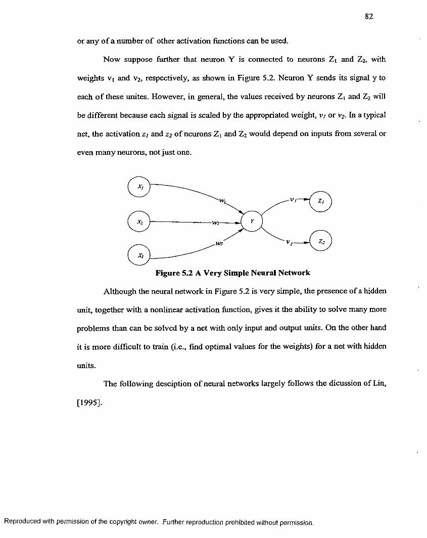
82
or any o f a number o f other activation functions can be used.
Now suppose further that neuron Y is connected to neurons Zi and Z2, with
weights Vi and v2, respectively, as shown in Figure 5.2. Neuron Y sends its signal y to
each o f these unites. However, in general, the values received by neurons Zj and Z2 will
be different because each signal is scaled by the appropriated weight, v/ or v2. In a typical
net, the activation z/ and z2 o f neurons Z\ and Z2 would depend on inputs from several or
even many neurons, not just one.
v,-w.
V,
Figure 5.2 A Very Simple Neural Network
Although the neural network in Figure 5.2 is very simple, the presence of a hidden
unit, together with a nonlinear activation function, gives it the ability to solve many more
problems than can be solved by a net with only input and output units. On the other hand
it is more difficult to train (i.e., find optimal values for the weights) for a net with hidden
units.
The following desciption o f neural networks largely follows the dicussion of Lin,
[1995].
Reproduced with permission of the copyright owner. Further reproduction prohibited without permission.
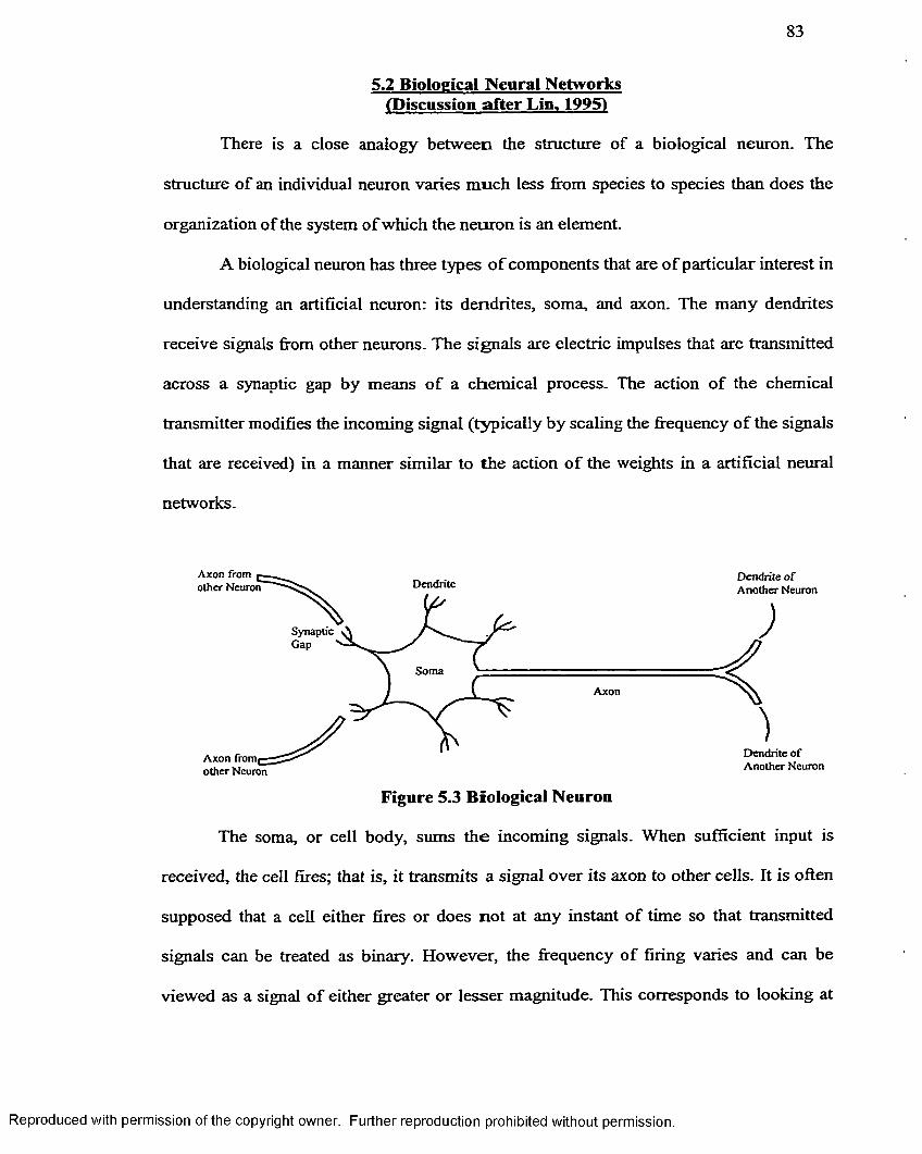
83
5.2 Biological Neural Networks (Discussion after Lin. 1995)
There is a close analogy between the structure of a biological neuron. The
structure o f an individual neuron varies much less from species to species than does the
organization of the system o f which the neuron is an element.
A biological neuron has three types o f components that are o f particular interest in
understanding an artificial neuron: its dendrites, soma, and axon. The many dendrites
receive signals from other neurons. The signals are electric impulses that are transmitted
across a synaptic gap by means o f a chemical process. The action o f the chemical
transmitter modifies the incoming signal (typically by scaling the frequency o f the signals
that are received) in a manner similar to the action o f the weights in a artificial neural
networks.
Axon from £ other Neuron
Dendrite of Another NeuronDendrite
SynapticGap
Soma
Axon
Dendrite of Another NeuronAxon from ^
other Neuron
Figure 5.3 Biological Neuron
The soma, or cell body, sums the incoming signals. When sufficient input is
received, the cell fires; that is, it transmits a signal over its axon to other cells. It is often
supposed that a cell either fires or does not at any instant of time so that transmitted
signals can be treated as binary. However, the frequency of firing varies and can be
viewed as a signal o f either greater or lesser magnitude. This corresponds to looking at
Reproduced with permission of the copyright owner. Further reproduction prohibited without permission.

8 4
discrete time steps and summing all activity (signals received or signals sent) at a
particular point in time.
The transmission o f the signal from a particular neuron is accomplished by an
action potential resulting from differential concentrations of ions on either side o f a
neuron’s axon sheath (the brain’s “white matter”). The ions most directly involved are
potassium, sodium, and chloride.
A generic biological neuron is illustrated in Figure 5.3, together with axons from
two other neurons and dendrites for two other neurons. Several key features o f the
processing elements o f artificial neural networks are suggested by the properties o f
biological neurons:
1. The processing element receives many signals;
2. Signals may be modified by a weight at the receiving synapse;
3. The processing element sums the weighted inputs;
4. Under appropriate circumstances (sufficient input), the neuron transmits a
single output;
5. The output from a particular neuron may go to many other neurons (the axon
branches).
Other features o f artificial neural networks that are suggested by biological neurons are:
6. Information processing is local (although other means of transmission, such as
the action o f hormones, may suggest means o f overall process control);
7. Memory is distributed:
a. Long-term memory resides in the neurons’ synapses or weights;
b. Short-term memory corresponds to the signals sent by the neurons;
Reproduced with permission of the copyright owner. Further reproduction prohibited without permission.

85
8. A synapse’s strength may be modified by experience;
9. Neurontransmitters for synapses may be excitatory or inhibitor.
Yet another important characteristic that artificial neural networks share with
biological neural systems is fault tolerance. A biological neural system is fault tolerant in
two respects. First, we are able to recognize many input signals that are somewhat
different from any signal we have seen before. Second, we are able to tolerate damage to
the neural system itself. Humans are bom with as many as 100 billion neurons. Most of
these are in the brain, and most are not replaced when they die. In spite o f our continuous
loss o f neurons, we continue to learn. Even in cases o f traumatic neural loss, other
neurons can sometimes be trained to take over the function o f the damaged cells. In a
similar maimer, artificial neural networks can be designed to be insensitive to small
damage to the network, and the network can be retrained in cases o f significant damage
(e.g., loss o f data and some connections).
Even for uses o f artificial neural networks that are not intended primarily to
model biological neural systems, attempts to achieve biological plausibility may lead to
improved computational features.
5.3 Fundamental feature of Neural Networks
Often, it is convenient to visualize neurons as arranged in layers. Typically,
neurons in the same layer behave in the same manner. Key factors in determining the
behavior o f a neuron are its activation function and the pattern o f weighed connections
over which it sends and receives signals. Within each layer, neurons usually have the
same activation function and the same pattern o f connection to other neurons. To be more
Reproduced with permission of the copyright owner. Further reproduction prohibited without permission.

86
specific, in many neural networks, the neurons within a layer are fully interconnected or
not interconnected at all. If any neuron in a layer (for instance, the layer o f hidden units)
is connected to a neuron in another layer, then each hidden unit is connected to every
output neuron.
The arrangement o f neurons into layers and the connection patterns within and
between layers is called the net architecture. Many neural nets have an input layer in
which the activation o f each unit is equal to an external input signal. The net illustrated in
Figure 5.2 has two layers of weights.
Wif
Wnt
■WijVV;
1m
W,Figure 5.4 Single-Layer Feed Forward Neuron Network
The single-layer and multilayer nets illustrated in Figures 5.4 and 5.5 are example
o f feed forward nets — nets in which the signals flow from the input units to the output
units in a forward direction. The fully interconnected competitive net in Figure 5.6 is an
example o f a recurrent net, in which there are closed-loop signal paths from a unit back to
itself
Reproduced with permission of the copyright owner. Further reproduction prohibited without permission.

87
5.4 Feed Forward Multilayer Neural Networks
A feed forward multilayer network is a net with one or more layers o f nodes (the
so-called hidden layers) between the input units and the output layer. Multilayer nets can
solve more complicated problems than can single layer nets, but training may be more
difficult. However, in some cases, training may be more successful because it is possible
to solve a problem that a single layer net cannot be trained to perform correctly at all.
.W pl
yWpk
w/«vv \
VS/,Vnl
up
Figure 5.5 A Multilayer Neural Network
Ou put
tnnut 2f n n t i t 1
Figure 5.6 Recurrent Neural Network
Reproduced with permission of the copyright owner. Further reproduction prohibited without permission.
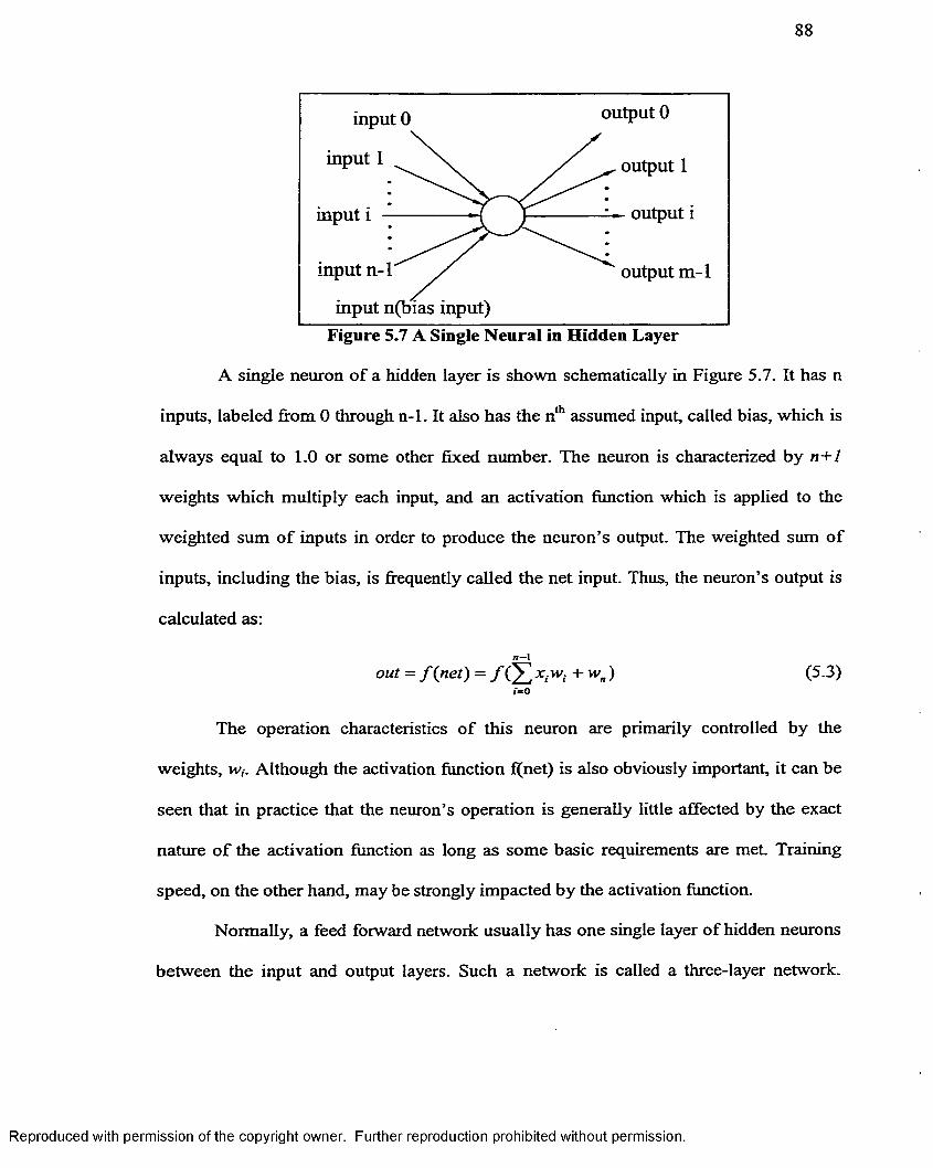
88
input 0 output 0
input 1 \. y ' output 1
input i ------------- -7 }— ■ output i
input n-1 y' output m-1
input n(bias input)Figure 5.7 A Single Neural in Hidden Layer
A single neuron o f a hidden layer is shown schematically in Figure 5.7. It has n
inputs, labeled from 0 through n-1. It also has the nth assumed input, called bias, which is
always equal to 1.0 or some other fixed number. The neuron is characterized by n+1
weights which multiply each input, and an activation function which is applied to the
weighted sum o f inputs in order to produce the neuron’s output. The weighted sum o f
inputs, including the bias, is frequently called the net input. Thus, the neuron’s output is
calculated as:
out = f (net) = / ( & , * , « . ) (5-3)«=0
The operation characteristics o f this neuron are primarily controlled by the
weights, w,. Although the activation function f(net) is also obviously important, it can be
seen that in practice that the neuron’s operation is generally little affected by the exact
nature o f the activation function as long as some basic requirements are met. Training
speed, on the other hand, may be strongly impacted by the activation function.
Normally, a feed forward network usually has one single layer of hidden neurons
between the input and output layers. Such a network is called a three-layer network.
Reproduced with permission of the copyright owner. Further reproduction prohibited without permission.

89
Rarely, two hidden layers will be needed. A four-layer network is shown schematically in
Figure 5.8.
5.4.1 Activation function
The activation function is a nonlinear function that, when applied to the net input of a
neuron, determines the output o f that neuron. Its domain must generally be all real
number, as there is no theoretical limit to what the net input can be. The range of the
activation function is usually limited. The most common limits are 0 — 1, while some
range from —1 — 1.
The majority o f current models use a sigmoid (S-shaped) activation function. A
sigmoid function may be loosely defined as a continuous, real-valued function whose
domain is real, whose derivative is always positive, and whose range is bounded. The
most commonly employed sigmoid function is the logistic function:
Output Layer
Input Layer
Hidden Layer 1
Hidden Layer 2
Figure 5.8 Four-Layer Feed Forward Neural Network
(5.4)
Reproduced with permission of the copyright owner. Further reproduction prohibited without permission.

90
One advantage o f this function is that its derivative is easily found:
/ ( x ) = / ( x ) ( l - / ( * ) ) (5.5)
It must be kept in mind that sigmoid functions never reach their theoretical
minimum or maximum. For example, neurons that use the logistic function should be
considered fully activated at around 0.9, and turn off at about 0.1 or so. It is futile to
attempt to train a network to achieve extreme values as its output.
a a. v p a f c a u v i i
The back propagation learning algorithm is a key feature o f most neural networks.
It has reawakened the scientific and engineering community to the modeling and
processing o f many quantitative phenomena using neural networks. This learning
algorithm is applied to multilayer feed forward networks consisting o f processing
elements with continuous differentiable activation functions. Such networks associated
with the back-propagation learning algorithm are also called back-propagation networks.
Given a training set o f input-output pairs, the algorithm provides a procedure for
changing the weights in a back-propagation network to classify the given input pattern
correctly. The basis for this weight update algorithm is simply the gradient-descent
method as used for simple perceptions with differentiable units.
For a given input-output pair (xfk), the back-propagation algorithm performs
two phases o f data flow. As a result o f this forward flow o f data, it produces an actual
output y .^ Then the error signals resulting from the difference between d,(k) and y (k) are
back propagated from the output layer to the previous layers update their weights. A three
layer network is shown in Figure 5.8. In Figure 5.8, the network has m nodes in the input
layer, 1 nodes in the hidden layer, and n nodes in the output layer; the solid lines show the
Reproduced with permission of the copyright owner. Further reproduction prohibited without permission.

91
forward propagation o f signals, and the dashed lines show the backward propagation o f
errors.
First consider an input-output training pair (xfk ) Given an input pattern x, a
node q in the hidden layer receives a net input of:
n e t P = S V * / (5-6)/= i
and produces an output of:
zq = f in e tq) (5.7)
The net input for a node in the output layer is then:
/ l mnett = Y Jwiqz<, = Z V £ V ; ) C5-8)
9=1 9=1 / = I
and it produces an output o f :
y,- = f i / i e t j ) = f ( ^ w iqz q) = / ( £ ^ / 2 v #j . ) ) (5.9)9 = 1 9 = 1 y=i
The above equations indicate the forward propagation o f input signals through the layers
o f neurons. Next, the error signals and their back propagation should be considered. First
define a error function:
= 4 zk - f ( p e u ) f - / ( t v , ) ? (5-io)»=I »=l ^ i=l 9 = 1
Then according to the gradient-descent method, the weights in the hidden-to-output
connections are updated by:
— (5.11)
Using Equations 5.8 — 5.10 and the chain rule, we have:
Reproduced with permission of the copyright owner. Further reproduction prohibited without permission.

92
A w ^ = - T ]"dE~ oy d(net;)
_di.net;) _ dw^= l\A i ~y,-] [ / ' ( .n e t , - ) [ z q ] = T ]8o iz (5.12)
where S01- is the error signal, and its double subscript indicates the ith node in the output
layer. The error signal is defined by:
dE dE dy.d{net,.) d(nett.)
(5.13)
where net, is the net input to node i o f the output layer, and f (net,) =df(netj)/d(netj). The
result thus far is identical to the delta learning rule obtained for a single-layer.
w
Figure 5.9 Three-Layer Back Propagation Network
For the weight update on the input-to-hidden connection, we can use the chain
rule with the gradient-descent method and obtain the weight update on the link weight
connecting node j in the input layer to node q in the hidden layer:
A v <„- = - ndE dE dE r d{netq )
. dv<u.— V dinetq) — 1 [ dinetq)_
(5.14)
Reproduced with permission of the copyright owner. Further reproduction prohibited without permission.

93
From Equation 5.10, it is clear that each error tem [dryi], i = 1,2, ...n, is a function o f z*,.
Evaluating the chain rule, we have:
Av«- = - y , ) / ' \ f ' (netq )x j (5-15)t= l
Using Equation 5.13, we can rewrite Equation 5.15 as:
Av« = = 7 Shqx j (5.16)i= l
where Suq is the error signal o f node q in the hidden layer and is defined as:
’■ Ti.net (5.16)dE dEd(netq ) A . d(netq) 1=1
where netq is the net input to the hidden node q. The error signal o f a node in a hidden
layer is different from the error signal o f a node in the output layer, as seen in Equations
5.13 and 5.17. Because o f this difference, the above weight update procedure is called the
generalized delta learning rule. We observe from Equation 5.17 that the error signal 5hq of
a hidden node q can be determined in terms o f the error signal 50i o f the nodes, y , that it
feeds. The coefficients are just the weights used for the forward propagation, but here
they are propagating error signals (50d backward instead of propagating signals froward.
This is shown by a dashed line in Figure 5.9. This also demonstrates one important
feature o f the back-propagation algorithm — the update rule is local; that is, to compute
the weight change for a given connection, we need only quantities available at both ends
o f that connection.
Note that both Equations 5.12 and 5.16 are in the same form o f the general weight
learning rule in Equation 5.10, except that the learning signals, r = 8, are different. The
above derivation can be easily extended to the network with more than one hidden layer
Reproduced with permission of the copyright owner. Further reproduction prohibited without permission.

94
by using the chain rule continuously. In general, with an arbitrary number o f layers, the
back propagation update rule in the form:
Aw- = rj8ix j = t]8output_ i x Xinput_f (5.18)
where output-i and input-j refer to the two ends o f the connection from node j to node i, xj
is the proper input-end activation from a hidden node or an external input, and 8 ; is the
learning signal which is defined by Equation 5.13 for the last (or output) layer o f
connection weights and defined by Equation 5.17 for all the other layers, When the
bipolar sigmoid function is used as the activation function, then Equations 5.13 and 5.17,
respectively, become:
(5.19)
and
(5 -2 0 >^ 1=1
In summary, the error back-propagation learning algorithm Back Propagation is shown
below.
Algorithm BP: Back-propagation Learning Rule
Consider a network with Q feedforward layers, q=l,2....Q , and let qnet[ and
denote the net input and output of the zth unit in the r̂th layer, respectively. The
network has m input nodes and n output nodes. Let qw,j denote the connection
weight from q~'yj to V i-
Input: A set o f training pairs { ( ^ ,ctk))\ k = 1,2,...p} where the input vectors are
augmented with the last elements as 1, that is, xfk)m+i=l.
Reproduced with permission of the copyright owner. Further reproduction prohibited without permission.

95
Step 0 (Initialization): choose rf>0 and Emax (maximum tolerable error). Initialize
the weightsto small random values. Set E =0 and k —l.
Step 1 (Training loop): Apply the &th input pattern to the input layer (q = l):
qy> = yi ~ x i ) for all i. (5.21)
Step 2 (Forward propagation): Propagate the signal forward through the network using:
ay, = a(q n e t,) = or(Y.q w / ' Y ) (5.22)j
for each i and q until the outputs o f the output layer ®y,- have all been obtained.
Step 3 (Output error measure): Compute the error value and error signals for
the output layer:
y , y + E (5-23>^ 1=1
- e y[) f \ Qneti) (5.24)
Step 4 (Error back-propagation): Propagate the errors backward to update the
weights and compute the error signals q_I5,- for the preceding layers:
A*w-. = TjqS r ly j and 9 w™ =q w°!d + A7w.. (5.25)
*-'5,. = f ' r ' n e t i ) Y dq»'jiqfij forq = Q ,Q -l,....2 . (5.26)
Step 5 (One epoch looping): Check whether the whole set o f training data has
been cycled once, If k<p, then k = k+1 and go to step 1; otherwise go to step 6 .
Reproduced with permission of the copyright owner. Further reproduction prohibited without permission.

96
Step 6 (Total error checking): Check whether the current total error is acceptable,
If E< Emax, then terminate the training process and output the final weights;
otherwise E = 0, and k = I , and initiate the new training epoch by going to step 1.
End BP
The above algorithm adopts the incremental approach in updating the weights;
that is the weights are changed immediately after a training pattern in presented. The
alternative is batch-mode training — where the weights are changed only after all the
training patterns have been presented. The relative effectiveness o f the two approaches
depends on the problem, but batch-mode training requires additional local storage for
each connection to maintain the immediate weight change. Furthermore, for best results,
patterns should be chosen at random from the training set instead o f following a fixed
order as in step 1 o f the algorithm BP.
Before discussing the convergence property o f the back-propagation learning
algorithm, we first take a look at the function approximation capability o f multilayer feed
forward networks. The following theorem addresses this issue which is presented and
proved in [Homik et al., 1989]
Theorem 5.1
Multilayer feed forward network architectures, with as few as one hidden layer
using arbitrary squashing activation functions and linear or polynomial integration
functions, can approximate virtually any (Borel-measurable) function o f interest
to any desired degree o f accuracy provided sufficiently many hidden units are
available. A function a: 9t -»• [0,1] ( or [-1.1] ) is a squashing function if it is non-
Reproduced with permission of the copyright owner. Further reproduction prohibited without permission.

97
decreasing, lim*.-**, f(A.) = 1, and f(A.) = 0 or (-1), where A. is a parameter
in the squashing function.
2Figure 5.10 Bipolar Sigmoid Function f ( x ) = ~ II + e ;
It is clear that the activation function defined in Equation 5.4 is a squashing
function. Theorem 5.1 establishes multilayer feed forward networks as a class of
universal approximators. This implies that any lack o f success in application must arise
from inadequate learning, insufficient numbers o f hidden units, or lack o f a deterministic
relationship between input and desired output. Although this theorem indicates that three
layers are always enough, some times it is essential to have four, five, or even more
layers in solving real world problems. This is because an approximation with three layers
would require an impracticably large number o f hidden nodes for some problem, whereas
an adequate solution can be obtained with a tractable network size by using more than
three layers.
Reproduced with permission of the copyright owner. Further reproduction prohibited without permission.

5.4.3 Learning Factors of Back Propagation
We shall address the issue o f convergence o f the back-propagation algorithm
based on some important learning factors such as the initial weights, the learning
constant, the cost function, the update rule, the size and nature o f the training set, and the
architecture (number o f layer and number o f nodes per layer). Our concern will focus on
the problems o f learning speed, local minima, and the generalization capability o f back-
propagation networks. Some variations on back propagation will also be introduced.
5.4.3.1 Initial Weights. The initial weights o f a multilayer feed forward network
strongly affects the ultimate solution. They are typically initialized at small random
value. Equal initial weight values cannot train the network properly if the solution
requires unequal weights to be developed. The initial weights cannot be large, otherwise
the sigmoid will saturate from the beginning, and the system will become stuck at a local
m i n i m u m or in a very flat area new the starting point. One proper way is to choose the
weight Wij in the range o f [ - 3 /A/^~,3/A/^~j, where k-t is the numbers of node that feed
forward to node i (the number o f input links o f node /).
5.4.3.2 Learning Constant (Learning Rate). Another important factor that
effects the convergence o f the back propagation learning algorithm significantly is the
learning constant 7 . There is no single learning constant value suitable for different
training cases, and 7 is usually chosen experimentally for each problem. A larger value of
7 could speed up the convergence but might result in overshooting, while a smaller value
o f 7 has a complementary effect. Values of 7 ranging from 10'3 to 10 have been used
successfully for many computational back-propagation experiments.
permission of the copyright owner. Further reproduction prohibited without permission.

99
Another problem is that the best values of the learning constant at the beginning
o f training may not be as good in later learning. Thus a more efficient approach is to use
an adaptive learning constant [Vogl et al., 1988; Jacobs, 1988]. The intuitive method is to
check whether a particular weight update has decreased the cost function. If it has not,
then the process has overshot, and q should be reduced. On the other hand, if several
steps in a row have decreased the cost function, then we may be too conservative and
should try increasing r|. More precisely, the learning constant should be updated
according to the following rule [Hertz.et al., 1991]:
A rJ =+ a i f AE < 0 consistently
— brj if AE> 0 (5.27)0 otherwise
where AE is the change in the cost function, and a and b are positive constants. The
meaning of “consistently” in Equation 5.27 can be judged based on the last k learning
steps or on a weighted moving average o f the observed AE.
S.4.3.3 Cost Functions. The quadratic cost function in Equation 5.10 is not the
only possible choice. The squared error term (dryd2 can be replaced by any other
differentiable function f(d,y) which is minimized when its arguments are equal. Based on
this new cost function, we can derive a corresponding update rule. It can be easily seen
that only the error signal 8oi in Equation 5.13 for the output layer changes for different
cost functions, while all the other equations of the back-propagation algorithm remain
unchanged.
The cost functions usually used are those based on Lp norm (/</? <" oo) because of
the advantage o f easier mathematical formulation. Such cost functions are in the form of:
Reproduced with permission of the copyright owner. Further reproduction prohibited without permission.

In particular, the least squares criteria used in the quadratic cost function is widely
employed because o f its simplicity.
S.4.3.4 Momentum. The gradient descent can be very slow if the learning
constant r\ is small and can oscillate widely if q is too large. This problem essentially
results from error surface valleys with steep sides but a shallow slope along the valley
floor. One efficient and commonly used method that allows a larger learning constant
without divergent oscillations occurring is the addition o f a momentum term to the
normal gradient-descent method (Palut et al., 1986). This idea is to give each weight
some inertia or momentum so that it tends to change in the direction o f the average
downhill force that it feels. This scheme is implemented by giving a contribution from
the previous time step weight change:
A w(t) = -rjVE (?) + aAw(t — 1) (5-30)
where 0< a < I is a momentum parameter, and a value o f 0.9 is often used. Figure 5.10
shows the trajectories o f gradient descent with and without momentum on a simple
quadratic surface. Note that the trajectory without momentum (the left curve) has larger
oscillations than the one with momentum (the right curves). We further observe from the
right curves in Figure 5.9 that the momentum can enhance progress toward the target
point if the weight update is in the right direction (point A to A’). On the other hand, it
can redirect movement in a better direction toward the target point in the case of
overshooting (Point B to B’). This observation indicates that the momentum term
Reproduced with permission of the copyright owner. Further reproduction prohibited without permission.

101
typically helps to speed up the convergence and to achieve an efficient and more reliable
learning profile.
—T\VE(t'+l) +<xAw(tr)
-T| V E (t+ I ) +aA w (f)
Figure 5.11 Gradient Descent on a Simple Quadratic Surface
5.4.3.5 Number of Hidden Nodes. The size o f a hidden layer is a fundamental
question often raised in the application of multilayer feedforward networks to real-world
problems. The exact analysis of this issue is rather difficult because o f the complexity of
the network mapping and the non-deterministic nature of many successfully completed
t r a i n i n g procedures. Hence, the size o f a hidden layer is usually determined
experimentally. One empirical guideline is as follows. For a network o f reasonable size
(e.g., hundreds or thousands of inputs), the size o f hidden nodes needs to be only a
relative small fraction of the input layer. If the network fails to converge to a solution, it
may be that more hidden nodes are required. If it does converge, fewer hidden nodes can
Reproduced with permission of the copyright owner. Further reproduction prohibited without permission.

102
be tried and then settle on a size based on overall system performance (Freeman and
Skapura, 1991).
5.43.6 Local Minimum. Every person charged with minimizing a function hopes
that it resembles a trampoline with a cannon ball resting in its center. Unfortunately, real-
life problems often have cross sections that look more like Figure 5.11. Obviously, any
algorithm that relentlessly crawls downward must have a very lucky starting position if it
is to settle into the lowest local minimum.
Avoiding false minima requires two separate procedures. First, we must avoid
starting in local minimum vicinity. Referring to the figure above, it behooves us to start
somewhere in the left half. If we settle into the broad minimum in the right half, it will be
very difficult to escape later. Second, we require a procedure for determining whether or
not we are in a local minimum and escaping if we are. This procedure will be
constructive in that we simply attempt to escape. If we succeed, we conclude that we
were in a local minimum. Otherwise, we assume that we have found the global minimum.
5.43.7 Local Minima Happen Easily. It is surprisingly easy for gradient
algorithms to get stuck in local minima when learning feed forward network weights.
Their error surfaces lend a whole new meaning to the term ill-conditioned. Even tiny
problems can sport local minima, and these minima can be very broad, attracting us in
from distant locations. This means that we should always repeat the learning process
from several different starting positions. It is reckless to use just one starting-weight
configuration, assuming that the minimum to which it leads is the best that we can do.
Reproduced with permission of the copyright owner. Further reproduction prohibited without permission

Neural networks always have many equally good global minima. This is because
o f the numerous symmetric inherent in the architecture. Swapping weight vectors among
hidden neurons obviously yields identical networks in terms of input/output mapping.
Other symmetries are possible. These multiple global minima are no problem and must
not be confused with the serious problem of inferior local minima.
Figure 5.12 A Typical Weight Surface Cross Section
Gori and Tesi, [1990] give a demonstration of just how easily local minima can
arise. The details in their proof are tedious and so will not be reproduced here. But one of
their main results is definitely worth presenting.
Consider the XOR problem. We have two inputs and one output, the training set
consist o f four cases, being each of the four possible combinations of 1 and 0 which the
two inputs can take on. The output is on if and only if exactly one of the two inputs is 1.
This is shown graphically in Figure 5.13. The four comer circles in that figure represent
the classical XOR problem
permission of the copyright owner. Further reproduction prohibited without permission.
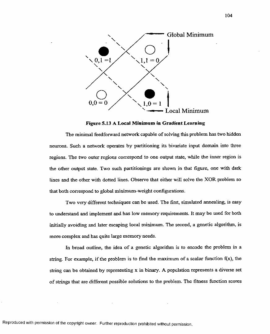
104
Global Minimum
— ■ Local Minimum
Figure 5.13 A Local Minimum in Gradient Learning
The minimal feedforward network capable o f solving this problem has two hidden
neurons. Such a network operates by partitioning its bivariate input domain into three
regions. The two outer regions correspond to one output state, while the inner region is
the other output state. Two such partitionings are shown in that figure, one with dark
lines and the other with dotted lines. Observe that either will solve the XOR problem so
that both correspond to global minimum-weight configurations.
Two very different techniques can be used. The first, simulated annealing, is easy
to understand and implement and has low memory requirements. It may be used for both
initially avoiding and later escaping local minimum. The second, a genetic algorithm, is
more complex and has quite large memory needs.
In broad outline, the idea o f a genetic algorithm is to encode the problem in a
string. For example, if the problem is to find the maximum of a scalar function f(x), the
string can be obtained by representing x in binary. A population represents a diverse set
o f strings that are different possible solutions to the problem. The fitness function scores
Reproduced with permission of the copyright owner. Further reproduction prohibited without permission.

105
each o f these as to its optimality. In the example, the associated value o f f for each binary
- string is its optimality. In the example, the associated value o f f for each binary string is
its fitness. At each generation, operators produce new individuals (strings) that are on
average fitter. After a given set o f generations, the fittest member in the population is
chosen as the answer.
aabcaabacbbcca " baccabbacccaaa
(a)
- — aabcccabaacaaa
(b)
—— aabcaaaacccaaa
(c)Figure 5.14 Genetic Operations on a Three-Letter Alphabet of {a,b,c}; (a) Crossover Swaps Strings at a Crossover Point; (b) Inversion Reverses the Order of Letters in
Substring; (c) Mutation Changes a Single Element
Genetic Algorithm can be decrbed as follow:
Choose a population size
Choose the number o f generations N
Initialize the population
Repeat the following for N generations
Iaabcaa[bacccaaabaeeabbacbbcca
i iaabcaabacocaaa
aabcaabacccaaa
Reproduced with permission of the copyright owner. Further reproduction prohibited without permission.

1. Select a given number o f pairs o f individuals from the population
probabilistically after assigning each structure a probability proportional to
observed performance
2. Copy the selected individuals, then apply operators to them to produce new
individuals
3. Select other individuals at random and replace them with the new individuals
4. Observe and record the fitness of the new individuals
Output the fittest individual as the answer
Genetic Operators are Crossover, Inversion Reverse and Mutation.
S.4.S.8 Simulated Annealing. Annealing is a term from metallurgy. When the
atoms in a piece o f metal are aligned randomly, the metal is brittle and fractures easily. In
the process o f annealing, the metal is heated to a high temperature causing the atoms to
shake violently. If it were cooled suddenly, the microstructure would be locked into a
random unstable state. Instead, it is cooled very slowly. As the temperature drops, the
atoms tend to fall into patterns that are relatively stable for that temperature. Providing
that the temperature drop is slow enough, the metal will eventually stabilize into an
orderly structure.
The analogue o f this process in optimization may be seen by examining Figure
5.12. Suppose one were to toss a ball onto that function and shake it strongly. After each
shake, the ball might land anywhere. If the strength o f the shaking is reduced, eventually
the ball will land somewhere in the right half and henceforth be unable to jump high
enough to move to the left half. If it lands in one of the small pockets in the right side,
relatively little shaking will be needed to toss it over the edge into a deeper pocket. Once
permission of the copyright owner. Further reproduction prohibited without permission.

down low, the relatively weak shaking will be unable to toss it into a higher pocket. Tf»is
process continues until it eventually settles into the lowest pocket.
Simulated annealing can be performed in optimization by randomly perturbing tlie
independent variables (weights in the case o f a neural network) and keeping track o f tlhe
best (lowest error) function value for each randomized set of variable. A relatively high
standard deviation for the random number generator is used at first. After many tries, the
set that produced the best function value is designated to be the center about whEch
perturbation will take place for the next temperature. The temperature (standard deviation
o f the random number generator) is then reduced and new tries done.
5.4.3.9 Choosing the Annealing Parameters. Each trial of a random weight se=t
can be very time consuming. Thus, we wish to use as few trials as possible. The total
number o f trails in our method is equal to the product o f the number of temperatures
times the number of iterations at each temperature. The obvious question is how we
choose each o f these quantities. Recall that after iterations at a particular temperature a re
complete. The best weights at that temperature become the center of iteration for the next
temperature. So we must consider how quickly we want to become locked into an area_
We also need to choose a starting and ending temperature.
The proper choice o f these quantities depends on our purpose. If we are initially
selecting weights for a starting point, we want to search a broad area. Also, we are not
interested in optimizing by slowly dropping the temperature. That task is best left to the
conjugate gradient algorithm. Thus we would choose very few temperatures. Two, o»r at
most three, are best. Also, a high starting and stopping temperature would be m ost
appropriate. On the other hand, if we have already progressed to a local minimum and. are
permission of the copyright owner. Further reproduction prohibited without permission.

trying to escape, it is better to use a few more temperatures, four or so. This is more
because o f the variety needed, rather than because we want to avail ourselves of the
optimization gained by many temperatures. We simply do not know how far we must
jump in order to escape the local minimum. It may be very broad, requiring a high
temperature. Or it may be a small pocket in a narrow channel. In this case, a high
temperature would nearly always toss us too far. By using a moderately high starting
temperature and a low stopping temperature, we are most likely to hit the lucky spot.
I f the optimization problem does not have a good direction solution, making
simulated annealing our only choice, then we must use many temperatures and cover a
wide range. The tradeoff now becomes one o f “How sure do we want to be that we have
the global m inim um ?” versus “How accurately do we need to estimate the minimum?” If
we prefer a rough approximation in exchange for high probability o f having the global
m inim um , the 5 to 10 temperature with a fairly high stopping temperature may be best.
On the other hand, if we need high accuracy, we are forced to use many temperatures and
drop low. The price we pay is less iteration at each temperature, making it more likely
that we will become trapped in a local minimum.
5.5 Neural Network Used in This Research
The neural network used in this research has three layers. Between the input layer
and the output layer there is one hidden layer. The input nodes are the microtunneling
project properties. They include microtunneling depth, microtunneling product pipe
diameter, ground water conditions, and soil properties. The output will be the ground
settlement at different points. The input layer has 10 nodes, the hidden layer has 100
permission of the copyright owner. Further reproduction prohibited without permission.

109
nodes, and the output layer has 10 nodes. Each node in the output layer represents the
ground settlement at a certain point.
Ground Settlement
Radius
Water Table
Ground Loss
Density
Bulk
Cohesion
Fnction Angle
Dilation Angle
Ground Settlement
Ground Settlement
Ground Settlement
Figure 5.15 Structure of Neural Network Used to Predict the Ground Settlement
5.5.1 Training Set Used to Train Neural Network
3dThe training sets used to train the neural network are the results o f the FLAC
program. Before training, 300 models have been set up with FLAC,3d and the results o f
these 300 models are used as training set of the neural network.
Several programs were written to speed up the research. First, a program was
written to generate the random input value for the neural network and FLAC.3D Because
no matter how humans choose, the random test value still contains bias. Using a program
can totally eliminate the bias. This program is written in Java (DataGen.java. Appendix
A).
Reproduced with permission of the copyright owner. Further reproduction prohibited without permission.

In order to allow these random selected data to be shared by the neural network,
FLAC30 and-other programs, these data are saved in a database.. This allows every client
program to use the same data and makes the data more organized.
DataFileGenJava (Appendix B) is the program which reads input data from the
database and generates a data file suitable for input into FLAC.3D DataFileGen.java is
listed in Appendix B, and a typical data file generated by DataFileGenJava is listed in
Appendix C.
FLAC3D runs each o f these data files that are generated by DataFileGenJava.
FLAC3D saves the ground settlement data into a data file. Another program ReadLog.java
(Appendix C) reads the ground settlement data from these data files and transfers the
settlement data into another format that is suitable to save in the database.
Although ground settlement data from FLAC3D is sufficient to describe the
ground profile, it does not always give the ground settlement value at the same fixed
distances from the centerline o f the pipe. Another program, LeastSquare.java (Appendix
D), uses a 10th degree polynomial to fit these data and generate ground settlement at the
fixed distances o f 0,1,2,3,...,9 meters from center line. These ground settlement data are
used to train the neural network.
Specifically 300 sets o f random site and project data was saved in the database.
The program used these 300 sets o f data to generate 300 data input files for FLAC.3D
Then FLAC3d ran these 300 data input files to get 300 sets o f settlement data, saved in
300 FLAC3D ground settlement output files. These 300 ground settlement data sets, at
variable distance from the centerline of the pipe, are then converted to 300 data sets
settlement at fixed distances o f 0,1,3,...9 meters from the centerline. These 300 sets o f
permission of the copyright owner. Further reproduction prohibited without permission.

I l l
settlement data are combined with their associated site, and project information is used as
the training sets for the neural network.
The inputs for the neural network are radius, depth, water table, ground loss, unit
weight o f soil bulk modulus o f soil, shear modulus o f soil, cohesion of soil, friction angle
o f soil, and dilation angle o f soil. These inputs and their range are listed in Table 5.1.
Table 5.1 Range of Microtunneling PropertiesPipe Radius (m) Depth (m) Ground Loss (%)
Min Value 0.15 2.0 1.0Max V alue 1.5 oa n 10.0
Table 5.2 Range of Soil PropertiesUnitWeight(kg/m3)
Young’sModulus(Mpa)
Poisson’sRatio
Cohesion(kPa)
FrictionAngle
DilationAngle
DenseSand
Min 1800 10.0 0.30 0 32° 0 °Max 2100 21.0 0.45 0 26° 10°
MediumSand
Min 1650 5.0 0.25 0 30° 0 °Max 1850 10.5 0.4 0 33° 10°
LooseSand
Min 1500 2.4 0.2 0 27° 0 °Max 1700 5.2 0.4 0 30° 10°
HardClay
Min 1800 48 0.2 48.0 0 ° 0 °Max 2100 191 0.5 100.0 0° 0 °
MediumClay
Min 1650 24 0.2 24.0 0° 0 °Max 1850 48 0.5 48.0 0° 0 °
SoftClay
Min 1500 12 0.2 12.0 0° 0 °Max 1700 24 0.5 24.0 0° 0 °
The range o f radius is between 0.15 meter and 1.5 meter. The range o f depth of
microtunneling is between 3.0 meters and 24 meter because typically few microtunneling
projects are carried out at the depth o f less than 3.0 meters or more than 24 meters.
Microtunneling projects at depth of less than 3.0 meters are seldom cost efficient
compared to open cut methods, and few sewer pipes are installed below 24 meters. The
Reproduced with permission of the copyright owner. Further reproduction prohibited without permission.

range o f ground loss is between 1% to 10%. The ground loss parameter is calculated with
the method mentioned in chapter 2 .-
The soil properties range is listed in Table 5.2. A program was written to select
soil properties randomly from Table 5.2. All these soil properties conform to values
provided in FLAC3D User Manual Volume I.
The back propagation learning algorithm used the gradient descent method to find
a local minimum. The back propagation algorithm trains the neural network by adjusting
the connection weight between each node. The magnitude of each adjustment can not be
too small or too large, and the magnitude heavily depends on the differential value o f
each node, f ( n e t inpul). This requires that the value o f the differential function can not be
too small or too large. A small differential value will make the back propagation very
slow to converge, and a large differential value will cause overshooting. The activation
function used in this neural network is logistic activation function.
If the input o f the derivative function is large (>5), the derivative function output
value will be very small. If this happens during training of the neural network, it will
cause the function not to converge or to converge very slowly.
There are two causes o f large input value o f derivative function in the neural
network used in this research. First, the absolute value of the input o f the neural network
is very large. For example, the soil density ranges from 1550 to 2100. This could cause
the hidden node input value to be very big. The input to the output layer node will also be
very large. Secondly, the hidden layer consists o f 100 nodes. This also will cause the
input to the output layer node to be very large. As mentioned before, a large input value
will cause the back propagation algorithm to converge very slowly.
permission of the copyright owner. Further reproduction prohibited without permission.

113
-frz-
Figure 5.16 Logistic Function
There are two methods to reduce a large input value problem. First, before we
input the input value o f neural network, we pre-process the input data to make it smaller.
For example, we divide the soil density value by 100 and divide the other input values by
proper factors. Second, we change the logistic function slope and use an adjusted logistic
function:
1/(* ) 1 + e—Jjc
(5.31)
where X is the coefficient to adjust the slope o f logistic function to make the slope smaller
around x = 0 and make the slope larger around x = ±co. This makes the drive value larger
even when the x is very large. But the trade o ff is that it makes the differential function
value smaller at x near 0 .
In this research, the pre-process input data method is used. The soil density value
is divided by 1000 to make the value between 1.55 to 2.1. Other input values are also pre-
processed in a similar manner.
Reproduced with permission of the copyright owner. Further reproduction prohibited without permission.

Then the back propagation method is used to train neural network using an
adaptive learning rate.
5.5.1.1 Initial Weight. The choice o f initial weights will influence whether the
net reaches a global (or only a locaL) minimum of the error and, if so, how quickly it
converges. The update o f the weight between two units depends on both the derivative of
the upper unit’s activation function and the activation of the lower unit. For this reason, it
is important to avoid choices o f initial weights that would make it likely that either
activation or derivatives o f activation, are zero. The values for the initial weights must not
be too large, or the initial input signads to each hidden or output unit will be likely to fall
in the region where the derivative o f the sigmoid function has a very high value (the so-
called saturation region). On the other hand, if the initial weights are too small, the net
input to a hidden or output unit will be close to zero, which causes extremely slow
learning. A common procedure is to initialize the weights (and bias) to random values
between -0.5 and 0.5 (or between —1 and 1 or some other suitable interval). The values
may be positive or negative because the final weights after training may be o f either sign
also.
A simple modification o f random initialization, developed by Nguyen and
Widrow, gives much faster learning. The approach is based on a geometrical analysis o f
the response of the hidden neurons to a single input; the analysis is extended to the case
o f several inputs by using Fourier transforms. Weights from the hidden units to the output
units (and bias on the output units) are initialized to random values between -0.5 and 0.5,
as is commonly used
with permission of the copyright owner. Further reproduction prohibited without permission

The initialization o f the weights from the input units to the hidden units is
designed to improve the ability o f the hidden units to Ieam. This is accomplished by
distributing initial weights and biases so that, for each input pattern, it is likely that the
net input to one o f the hidden units will be in the range in which that hidden neuron will
learn most readily. The definitions we use are as follows:
n number o f input units
p number o f hidden units
p scale factor: f3 — 0 .7(p)u" =0.7^[p
The procedure consists o f the following simple steps:
for each hidden unit j :
initialize its weight vector (from the input units);
weighty = random number between — 0.5 and 0.5 (or between -y and y).
Compute jjvy(old)|| = ^ v 1; (oW) 2 +vzj(old) 2 +... + vnj{old) 2
Reinitialize weights:
v . (5.32)IM°W>I1
Set bias:
vOJ- = random number between -P and P
The use o f Nguyen-Widrow initialization not only improved the training speed
but also greatly reduced the chances o f generating initial weights for which the neural
network fails to converge.
In Chapter 4, Numerical Approach, the effect of all the ten factors is examined. It
shows that the microtunneling depth, product pipe diameter, and ground loss have larger
with permission of the copyright owner. Further reproduction prohibited without permission.

impact on the final ground settlement than any other factor. If the weights, which connect
these three inputs o f the neural network, have a higher value than the other weights, the
network will converge faster. So in this research, the weights connecting these three
inputs have a slightly higher initial weight value than the other weights.
5.5.1.2 Number of Hidden Layers. The size o f a hidden layer is a fundamental
question often raised in the application o f multilayer feed forward networks to real-world
problems. The exact analysis of this issue is rather difficult because o f the complexity o f
the network mapping and nodeterministic nature o f many successfully completed training
procedures. Hence the size o f a hidden layer is usually determined experimentally. One
empirical guideline is as follows: For a network o f reasonable size (e.g., hundreds or
thousands o f inputs), the size o f hidden nodes needs to be only a relatively small fraction
o f the input layer. I f the network fails to converge, fewer hidden nodes are tried, and then
a size is chosen based on overall system performance.
In this research, the hidden layer contain 100 nodes. This number was selected
based on hundreds o f tests. Almost every number o f hidden node between 50 to 150 was
tested. A hidden layer with 100 nodes was selected based on overall system performance.
5.5.13 Desired Output Data. The neural network outputs are ground surface
settlements at 10 points. These points are the points 0, 1,2, 3, 4, 5, ...9 meters from the
centerline o f the pipe. Since the theoretical ground settlement profile of microtunneling
project is symmetric, based on these 10 ground settlement values, we can get the ground
settlement profile on both side o f the pipe with a total width of 18 meters. This profile o f
settlement profile is typically networks give is typically enough for engineering use.
with permission of the copyright owner. Further reproduction prohibited without permission.

Some values o f the desired outputs are too small to allow effective training o f the
neural network. As stated before, if the output o f an activation function is too small or too
large, it will cause the derivative to be value too small to be used to update the weights.
So before the raw ground settlement data were used, they were normalized to the interval
between 0 to 1 by the equation 5.33:
old initial output — min outputdesired_output = ----=------=— ----------- =— - — (5.33)max_output — min_output
After processed by equation 5.33, there would be still be some values that are too
small. These values are treated by equation 5.34 again to make sure no value is too small.
After processing the output value using equation 5.34, the ground settlement value
(desired neural network output value) would be at least 0.3. These values allow the
derivative value of the activation function to have a suitably large value to training the
neural network:
desire output +0.5 _ _new _ desire _ output = ------- ~ 1 5------------- (5-34)
5.5.1.4 Local Minimum. To avoid a local minimum, this neural network used
simulated annealing. There is rarely any need for extremely large weights. In fact, large
weights can lead to extreme activation levels (near the theoretical limits of the activation
function). This is turn gives rise to very small derivatives o f the activation function,
which in turn tends to paralyze that weight. At each stage, a new random perturbation
should not exceed 1. Each new value should be tested against the absolute upper limit.
The absolute value of the new weight should not be allowed to exceed this limit. A limit
o f 1 in this network is sufficiently large to permit wide variation, yet small enough to let
gradient techniques pull it in later if necessary.
permission of the copyright owner. Further reproduction prohibited without permission.

The first step in the annealing is to copy the input guess v and w matrix to the
work matrix-center_v and center_w. The objective function is evaluated at this guess, and
the function value preserved as the best so far. The standard deviation o f the random
perturbation initialized to the user’s starting temperature, and the reduction factor is
computed.
At the start o f each pass through the temperature loop, the improved flag is set to
zero. When all iterations at that temperature are complete, the perturbation center for the
next temperature w ill be updated only if that flag was set to 1 due to improvement.
Otherwise, the same center will be used again.
The function shake is used to perturb around the center point. It sums uniform
deviates to realize a more bell shaped curve than would be attained with one deviate
alone. By adding two and subtracting two, the random variable has mean zero.
I f the new trial point has a superior function value, update the best function value
and save the weight matrix. Set improved flag to indicate that we has a success at this
temperature. If the function has been minimized enough to suit the user, break out o f the
loop. Finally, set back the iteration counter to give us more tries at this temperature,
Regardless o f whether o f not we improved, verify that we have not called the objective
function the limiting number o f times.
When all iterations at a temperature are complete, test the improved flag. If we
improved, set the w ork weight matrix to the best weight matrix.
permission of the copyright owner. Further reproduction prohibited without permission.

5.6 Results
The training o f neural network was carried out on a personal computer with a
Pentium III processor operating at 500 MHz, 128 MB memory, and the operating system
Windows NT 4.0. The total training time was about 26 hours. The average error is about
0.02mm. The absolute error ranges from 0 mm to 0.5 mm, and the relative error ranges
from 0% to 55%. The high relative error only occurs at small ground settlement, in test
data 4, in which the desired output o f the neural network is 0.052 cm, the real output is
0.0807 cm, the absolute error is 0.029 cm, and the relative error is 55%. Even though the
relative error is high when ground settlement is small, it does not harm the whole
performance o f the neural network because in small settlements even with large relative
error, the neural network error is still small. The typical relative error ranges from 1% to
6.5%.
Test data 1: In Figure 5.17 the input data is: Radius 1.0275 meter, depth 16.65
meter, ground water depth 23.86 meter, ground loss 9.55%, soil unit weight 2045 kg/m,3
bulk modulus 9.92 kPa, shear modulus 4.78 kPa, cohesion 5 MPa, friction angle 27.5,°
dilation angle 0.° The ground settlement predicted by FLAC3D is listed in the first column
of Table 5.3, and the ground settlement predicted by the neural network is listed in the
second column.
with permission of the copyright owner. Further reproduction prohibited without permission

120
Table 5.3 Ground Settlement Data o f FLAC3D and Neural Networks (Test ___________________ Data 1) __________________________
. . . . » .—n +n IJ r t f '•»11 /sfDistance from center line Result o f FLACJU R esult o f neural network(m) (cm) (cm)0 1.203 1.24I 1.203 1.2622 1.194 1.2283 1.178 1.2204 1.155 1.2055 1.128 1.1546 1.096 1.1177 1.062 1.0628 1.026 1.0139 0.988 0.967
1.4
1.2
0.8 FLAC 3d Neural Network0.6
0.4
0.2
10
Distance from Centerline (m)
Figure 5.17 Ground Settlement Result of FLAC30 and Neural Network (Test Data 1)
Test data 2: In Figure 5.18, the input data is: Radius 1.0275 meter, depth 19.85
meter, ground water depth 20.44 meter, ground loss 9.1%, soil unit weight 1687.5 kg/m,3
bulk modulus 5.38 MPa, shear modulus 3.39 MPa, cohesion 5 MPa, friction angle 32.5,°
dilation angle 10.° The ground settlement predicted by FLAC3D is listed in the first
column of Table 5.4, and the ground settlement predicted by the neural network is listed
in the second column.
Reproduced with permission of the copyright owner. Further reproduction prohibited without permission.

121
Table 5.4 Ground Settlement Data of FLAC3P and Neural Networks (Test Data 2)Distance from center line
(m)Result o f FLACJu
(cm)Result o f neural network
(cm)0 1.103 1.0581 1.103 1.0652 1.098 1.0733 1.087 1.0644 1.072 1.0535 1.053 1.0356 1.031 1.0137 1.006 0.9758 0.980 0.9459 0.952 0.906
1.2
0.8FLAC 3d Neural Network
0.6
0.4
0.2
Distance from Centerline (m)
Figure 5.18 Ground Settlement Result of FLAC3D and Neural Network (Test Data 2)
Test data 3: Radius 1.095 meter, depth 20.85 meter, ground water depth 1.82
meter ground loss 6.4%, soil unit weight 1660 kg/m3, bulk modulus 14.53 MPa, shear
modulus 9.897 MPa, cohesion 1 MPa, friction angle 15,° dilation angle 0.° The ground
settlement predicted by FLAC3D is listed in the first column o f Table 5.5, and the ground
settlement of predicted by the neural network is listed in the second column.
Reproduced with permission of the copyright owner. Further reproduction prohibited without permission.

122
Table 5.5 Ground Settlement Data o f FLAC30 and Neural Networks (Test DataD istance from center line
(m)R esu lt o f FLACJb
(cm)Result o f neural netw ork
(cm)0 0.219 0.233I 0.219 0.2332 0.218 0.2273 0.216 0.2324 0.213 0.2245 0.209 0.2146 0.204 0.2117 0.199 0.2068 0.193 0.1909 0.188 0.185
3)
0.25
0.2
0.15 FLAC 3d Neural Network
0.1
0.05
Distance from Centerline (m)
Figure 5.19 Ground Settlement Result of FLAC3D and Neural Network (Test Data 3)
Test data 4: Radius 0.555 meter, depth 20.85 meter, ground water depth 5.55
meter, ground loss 1%, soil density 1632.5 kg/m ,3 bulk modulus 32.93 MPa, shear
modulus 7.25 MPa, cohesion 8 MPa, friction angle 31.25,° dilation angle 10.° The
ground settlement predicted by FLAC30 is listed in the first column o f Table 5.4, and the
ground settlement predicted by the neural network is listed in the second column.
Reproduced with permission of the copyright owner. Further reproduction prohibited without permission

123
Table 5.6 Ground Settlement Data o f FLAC30 and Neural Networks (Test Data 4)Distance from center line
(m)Result o f FLAC3 u
(cm)Result of neural network
(cm)0 0.052 0.0801 0.050 0.0792 0.046 0.0733 0.041 0.0604 0.036 0.0535 0.031 0.0416 0.027 0.0337 0.023 0.0338 0.020 0.0239 0.017 0.025
_ 0.09f 0.08r o.o7I 0.06®c ®<0■o 0.03
0.02 O 0.01
0.050.04
c32
102 80 4 6
Distance from Centerline (m)
FLAC 3d Neural Network
Figure 5.20 Ground Settlement Result of FLAC30 and Neural Network (Test Data 4)
Test data 5: Radius 1.0275 meter, depth 20.85 meter, ground water depth 20.757
meter, ground loss 4.15%, soil density 1770 kg/m ,3 bulk modulus 28.15 MPa, shear
modulus 12.25 MPa, cohesion 5.5 MPa, friction angle 25,° dilation angle 0.° The ground
settlement predicted by FLAC3D is listed in the first column of Table 5.7, and the ground
settlement predicted by the neural network is listed in the second column.
Reproduced with permission of the copyright owner. Further reproduction prohibited without permission.

124
Table 5.7 Ground Settlement Data of FLAC30 and Neural Networks (Test Data 5)Distance from center line Result of FLAC5b Result o f neural network
(m) (cm) (cm)0 0.522 0.5341 0.523 0.5332 0.521 0.5293 0.517 0.5244 0.511 0.5175 0.503 0.5046 0.494 0.4937 0.484 0.4768 0.473 0.4619 0.462 0.444
0.6
0.5
0.4FLAC 3d Neural Network
0.3
0.2
0.1
10
Distance from Centerline (m)
Figure 5.21 Ground Settlement Result of FLAC30 and Neural Network (Test Data 5)
Test data 6 : Radius 0.42 meter, depth 15.6 meter, ground water depth 13.14
meter, ground loss 5.95%, soil density 1550 kg/m ,3 bulk modulus 34.52 MPa, shear
modulus 11.93 MPa, cohesion 9.5 MPa, friction angle 18.75,° dilation angle 10.° The
ground settlement predicted by FLAC3D is listed in the first column of Table 5.8, and the
ground settlement predicted by neural network is listed in the second column.
Reproduced with permission of the copyright owner. Further reproduction prohibited without permission

125
Table 5.8 Ground Settlement Data of FLAC3P and Neural Networks (Test DataDistance from center line Result o f FLAC30 Result o f neural network
(m) - (cm) - (cm) -0 0.205 0.1871 0.205 0.1912 0.203 0.1933 0.200 0.1934 0.196 0.1945 0.191 0.1966 0.186 0.1907 0.180 0.1878 0.174 0.1829 0.168 0.170
6)
0.6
0.5
0.4FLAC 3d Neural Network
0.3
0.2
0.1
10
D istance from C enterline (m)
Figure 5.22 Ground Settlement Result of FLAC30 and Neural Network (Test Data 6)
Test data 7: Radius 0.8925 meter, depth 12.45 meter, ground water depth 6.56
meter, ground loss 4.15%, soil density 1935 kg/m ,3 bulk modulus 23.78 MPa, shear
modulus 12.59 MPa, cohesion 8 MPa, friction angle 32.25,° dilation angle 0.° The ground
settlement predicted by FLAC3D is listed in the first column of Table 5.9, and the ground
settlement predicted by the neural network is listed in the second column.
Reproduced with permission of the copyright owner. Further reproduction prohibited without permission

126
Table 5.9 Ground Settlement Data of FLAC30 and Neural Networks (Test Data 7)Distance from center line R esult o f FLAC3u R esult o f neural network
(m ) - (cm) - (cm).0 0.410 0.4271 0.409 0.4252 0.402 0.4113 0.392 0.3944 0.378 0.3785 0.362 0.3546 0.345 0.3377 0.327 0.3208 0.309 0.2939 0.292 0.279
0.450.4
~ 0.35o 0.3| 0.25® 0.2 w■o 0.15
0.1 ® 0.05
3Ow
102 4 6 8
D istance from Centerline (m)
- • — FLAC 3d —•" N e u ra l Network
Figure 5-23 Ground Settlement Result of FLAC30 and Neural Network (Test Data 7)
Test data 8 : Radius 1.43 meter, depth 15.60 meter, ground water depth 22.45
meter, ground loss 7.75%, soil density 2017.5 kg/m,3 bulk modulus 16.27 MPa, shear
modulus 7.83 MPa, cohesion 2 MPa, friction angle 23.75,° dilation angle 10.° The ground
settlement predicted by FLAC3D is listed in the first column o f Table 5.10, and the
ground settlement o f neural network is listed in the second column.
Reproduced with permission of the copyright owner. Further reproduction prohibited without permission.

127
Table 5.10 Ground Settlement Data o f FLAC30 and Neural Networks (Test Data 8)Distance from center line Result o f FLAC3b Result o f neural network
(m)- (cm)- (cm)0 0.986 0.9731 0.986 0.9782 0.977 0.9583 0.961 0.9414 0.939 0.9195 0.913 0.8836 0.882 0.8567 0.850 0.8168 0.815 0.7809 0.780 0.748
1.2
0.8
0.6
0.4
0.2
0106 820 4
Distance from Centerline (m)
- • —FLAC 3d ~ N e u r a l Network
Figure 5.24 Ground Settlement Result of FLAC30 and Neural Network (Test Data 8)
After comparing the FLAC3D result and neural network result, the neural network
can represent the FLAC3D ground settlement predictions accurately. The maximum
absolute error is less than 0.1 cm. This error is acceptable in engineering practice.
Compared to theoretical method, empirical method and numerical method, the neural
network approach has several advantages over other method:
• Includes more soil and project parameters than the theoretical method
• Much faster than the numerical method
Reproduced with permission of the copyright owner. Further reproduction prohibited without permission.

128
• Easy to us* e. User does not need to understand neural networks
• Suitable fo r a larger range o f soil types
5.7 Case Histories
The microtumneling experiments carried out at Waterways Experment Station
provided some ground settlement data [Bennett, 1997]. The experimental data, FLAC3D
result, neural networfk result and calculation result provide by Bennett [1997] are shown
in Figures 5.25, 5.2*6, and 5.27. The method used by Bennett to calculate the ground
settlement was the ermperical method.
Case 1: The so il type is sand, microtunneling depth is 2.7405 meter, pipe diameter
is 66.04 cm and groinnd loss is 5.8% o f microtunneling cutting face. Ground water table is
below the pipe, soil 'unit weight is 1630 kg/m3, bulk modulus is 16.0 Mpa, shear modulus
is 12.5 Mpa, cohesiron is 0, friction angle is 37°, dilation angle is 0°.
Case 2: The soil type is clay, microtunneling depth is 2.436 meter, pipe diameter
is 66.04 cm and gromind loss is 5.8% o f microtunneling cutting face. Ground water table is
below the pipe, so*il unit weight is 1401 kg/m3, bulk modulus is 0.833 Mpa, shear
modulus is 0.384 MIpa, cohesion is 8kPa, friction angle is 0°, dilation angle is 0°.
Case 3: Thee soil type is clay gravel, microtunneling depth is 2.436 meter, pipe
diameter is 66.04 c m and ground loss is 5.8% o f microtunneling cutting face. Ground
water table is be low the pipe, soil unit weight is 1868 kg/m3, bulk modulus is 0.8 Mpa,
shear modulus is 0.2384 Mpa, cohesion is 0, friction angle is 37°, dilation angle is 0°.
The compamson of the results o f FLAC3D, neural network, measured settlement
and calculated settlem ent (empirical method) shows that the FLAC3D and neural network
Reproduced with permission of the copyright owner. Further reproduction prohibited without permission

129
can predict the ground settlement associated with microtunneling reasonably well overall
and to a better degree than the empirical method
f.4
FUVC3D
♦ " N e u ra l Network A Measured Min ■*- Measured Max ♦ " B e n n e tt
• 0.8
0.4
0.2
85 7 9 1060 2 3t 4
D istance from Centerline (m)
Figure 5.25 Ground Settlement in Sand
1.4
FLAC3D ■•“ Neural Network * Mearued Min
Measured Max ■♦“ Bennett_______
• 0.8
0.4
8 9 105 6 730 41 2
Distance from Centerline (m)
Figure 5.26 Ground Settlement in Clay
Reproduced with permission of the copyright owner. Further reproduction prohibited without permission.

130
FLAC3D0.9
N eural N etw ork
A M e aru e d Min0.8
Measured Max0.7 B e n n e tt
~ 0.6
5 0.5
0.4
0.3
0.1
95 7 8 1062 3 41
Distance from Centerline (m)
Figure 5.27 Ground Settlement in Clay Gravel
Reproduced with permission of the copyright owner. Further reproduction prohibited without permission.

CHAPTER 6
CONCLUSIONS & RECOMMENDATIONS
In this research, the ground settlement associated with microtunneling is studied
using a theoretical approach, an empirical approach, numerical simulation, and an
artificial intelligence approach to reproduce quickly the result o f numerical simulation.
The theoretical approach is based on the equivalent ground loss [Lee, 1989] and
point ground loss [Sagaseta, 1987] concept. It can predict the ground settlement with one
simple equation, but it does not consider the effect o f varying soil properties. Because o f
its limitations, it is principally a good method to check against the other methods.
The empirical approach is based on large diameter tunneling case histories, and it
is widely used in predicting the ground settlement associated with large diameter
tunneling. This approach appears to provide satisfactory results in normally consolidated
clays but tends to be misleading in granular soils [New and O’Reilly, 1991] and also in
overconsolidated clays [Eisenstein et al., 1981]. Although some aspects o f
microtunneling are similar to large diameter tunneling, microtunneling is a significantly
different technique in terms o f its pipe jacking procedure and remote control steering. No
information was found in the literature indicating the accuracy of the empirical method
for predicting the ground settlement associated with microtunneling.
131
permission of the copyright owner. Further reproduction prohibited without permission.

The numerical simulation approach in this thesis uses the finite difference method
to predict-the ground settlement associated with microtunneling. Numerical methods can
provide results that agree reasonably with the results from field data provided the ground
loss data is known but, in general, the simulated ground settlement trough appears to be
wider than the results observed in the field. The drawbacks o f numerical methods include
the problems that, firstly, the user must at least have some knowledge about the
simulation process and have spent some time in learning how to use the numerical
method software; and, secondly, the user has to wait for a long time for the result o f a
single numerical simulation.
Using numerical simulation coupled with an artificial intelligence approach, a
feed forward neural network that can provide the ground settlement profile was
developed to predict the ground settlement associated with microtunneling. Input data
required for the neural network are the soil and project parameters plus the equivalent
ground loss parameter that can be calculated with method provided in chapter 2. The
training o f the neural network used a back propagation learning algorithm on training
data developed from the numerical simulation. After 26 hours of training, the neural
network can predict the settlement very closely. The neural network developed was tested
on the same problem against a commercial neural network software and the neural
network developed in this research had much lower errors than the commercial software
because it is specifically optimized for this particular problem.
The neural network method has several advantages. Firstly, the neural network
developed can provide an estimate derived from a wide range o f site and project
parameters. Secondly, the neural network can provide results immediately. Thirdly, the
permission of the copyright owner. Further reproduction prohibited without permission.

133
neural network method is easy to use. The user does not need to understand how the
neural network works and/or prepare complicated input data files. The method can be
used to understand the extent c f ground loss that may cause damaging surface settlement
under particular site conditions by varying the unknown or critical parameters. This, in
turn, can be used to guide operational practice on critical microtunneling projects.
Reproduced with permission of the copyright owner. Further reproduction prohibited without permission.

CHAPTER 7
FURTHER WORK
7.1 Measurement of Ground Loss
Although we can predict the ground movement from the soil loss parameter with
reasonable accuracy, the estimation o f a soil loss, especially that includes the most
damaging condition o f extensive soil loss at the face, is very difficult. The soil loss is
affected by many factors such as soil characteristics, ground water level, microtunneling
machine advance speed, tail void, and the presence and position o f other underground
structures. Nevertheless, because o f its speed o f prediction, the neural network approach
developed in this thesis could be used effectively in the on-site prevention o f damaging
ground movements — if we can measure the soil loss at the face in real time in the
microtunneling machine.
In order to measure the soil loss in microtunneling machine, we need to measure
the difference in mass per unit volume between the incoming slurry and the outcoming
slurry. For income slurry weight we have:
= y,v. (7.1)
where W,- is the incoming slurry weight during microtunneling machine advance of one
unit length, y,- is the incoming slurry density, and v,- is incoming slurry volume in one unit
time.
For outgoing slurry weight we have:
134
permission of the copyright owner. Further reproduction prohibited without permission.

135
W 0 = y 0v 0 (7 .2 )
where W0 is outgoing slurry weight, y0 is the outgoing slurry density, v0 is outgoing slurry
volume in one unit time, and vm is the advance speed o f microtunneling machine.
W0-Wi is the weight o f soil lost in the microtunneling process. So the volume of
the soil lost in microtunneling machine is:
r * . = ( K - ^ . O-3)
where V[oss is the volume o f soil lost in the microtunneling process. In order to get the
volume o f soil loss, we must add in the soil loss cause by the tail void, which is:
r tv= ^ ( /? 2 - r 2)vm (7.4)
The R and r are the outside diameter o f the microtunneling machine and the permanent
pipe respectively, and vm is the advance speed o f microtunneling machine. So the Vs is:
V, = V:oss +Vn =iW0 - W i) - n r 2vm (7.5)
7.2 Prediction o f Ground Settlement in Real Time
If a flow meter can be developed, as indicated above, that can measure the density
and velocity o f the slurry flow in real time, a control system can be used to provide
feedback to the microtunneling machine. The density and velocity of the income and
outcome slurry flow provide data on the ground mass removed by microtunneling
machine. This can be compared with the volume represented by the physical machine
advanc provided that the density o f soil around the microtunneling can be estimated
before the microtunneling work. Adding the volume changes caused by the annular
space, machine attitude, etc, the short-term ground settlement prediction for a
microtunneling project could be updated in real time as site data was collected. This
Reproduced with permission of the copyright owner. Further reproduction prohibited without permission.

136
would provide a means o f initial prediction o f ground movements prior to the project and
updating o f these projections in real time based on machine performance data and soil
conditions obtained on site.
Reproduced with permission of the copyright owner. Further reproduction prohibited without permission.

REFERENCES
Anagnostou, G. and Kovari, K (1994) “ The Face Stability o f Slurry-Shield-Driven Tunnels” Tunnelling and Underground Space Technology Vol. 9 No.2 April. 1994
Attewell, P. B. 1978. “ Ground movements caused by tunnelling in soil” Proc. Conf. On Large Ground Movements and Structures, Cardiff 1977. P812-948. London: Pentech Press.
Attewell, P. B. and Selby, A. R. (1989) “ Tunnelling in Compressible Soils: Large Ground Movements and Structural Implications” Tunnelling and Underground Space Technology Vol. 4 No. 4
Bennett, R. D., and Taylor, P. (1993). “Construction o f Microtunneling test facility at WES and preliminary Test Results” Construction Productivity Advancement Research (CPAR) p r o g r a m . Trenchless Technology Center, Louisiana Tech University, Ruston, LA
Bennett, R. D., and Staheli, K. (1997) “Controlled Field Tests o f Retrievable Microtunneling System with Reaming Capabilities” Construction Productivity Advancement Research (CPAR) Program, CPAR-GL 97-1, May 1997
Bennett, R. D. (1998) “Jacking Loads and Ground Deformations Associated with Microtunneling” Ph.D. Thesis Univeristy o f Illinois at Urbana-Champaign
Bennett, R. D., Guice L. K., Khan, S. and Staheli, K. (1995) “Guidelines for Trenchless Technology: Cured-in Place Pipe (CIPP), Fold and Formed Pipe (FFP) Mini-Hoaizontal Directional Drilling (mini-HDD) Microtunneling” TTC Technical Report #400
Cording, E. J., and Hansmire, W. H. (1975) “Displacement around soft ground tunnels, General Report: Session IV, Tunnels in soil.” Proceeding 5th Panamerican Congr. on soil Mechanics and Foundation Engineering
Eisenstein, Z., El-Nahhas, F., and Thomson, S. (1981). “Strain field around a tunnel in stiff soil” Proc. 10th Int. Conf. on Soil Mech. and Found. Engineering. Vol. 1, A. A. Balkema, Rotterdam, The Netherlands
Freeman, J. A., and Skapura, D. M. (1991) “Neural networks: algorithm, applications, and p r o g r a m m i n g techniques.” Reading, MA: Addison-Wesley
137
Reproduced with permission of the copyright owner. Further reproduction prohibited without permission.

138
Hertz, J., Krogh, A. and Palmer, R. G. (1991) “Introduction to the theory o f neural computation”, New York, Addison-Wesley
Homik, K., Stinchcommbe, M. “Multilayer feedforward networks are universal approximators.” Neural Networks 2:359-366
Hurrell, M.R. (1985). “ The empirical prediction o f long-term surface settlements above shield-driven tunnels in soil” Ground Movements and Structures: Proc. 3rd Int. Conf., Cardiff 1984. P161-170. London: Pentech Press
Jacobs, R. A. (1988) “Increased rates o f convergence through learning rate adapation.” Neural Networks 1: 295-307
Klein, S. J. (1995) “Design Aspects o f Microtunneling Projects” NO-DIG Engineering Vol. 2, No. 2 summer 1995 p.9-12
Lee, K. M. 1989. “Prediction o f ground deformations resulting from shield tunneling in soft clays.” Ph.D. thesis, The University o f Western Ontario, London, Ont.
Lee, K. M., and Rowe, R. K. (1990a) “Finite element modeling o f the three-dimensional ground deformations due to tunneling in soft cohesive soils. Part I. Methods o f analysis.” Computers and Geotechnics. 10(2): 87-110
Lee, K. M. and Rowe, R. K. (1990b) “Finite element modeling o f the three-dimensional ground deformations due to tunneling in soft cohesive soils. Part II. Results.” Computers and Geotechnics. 10(2): 87-110
Lo, K. Y., and Rowe, R. K. (1982) “Prediction o f ground subsidence due to tunneling in clays” Research Report GEOT-10-82, Faculty o f Engineering Science, The University of Western Ontario, London, Ont.
Lin, C. T. and Lee, C. S. G. (1996) “Nural Fuzzy Systems” Prentice-Hall, Inc. Upper Saddle River, NJ
Loganathan, N. and Poulos, H. G. (1998) “ Analytical Prediction for Tunneling-Induced Ground Movements in Caly” Journal o f Geotechnical and Geoenvironmental Engineering, Vol 124 No. 9
New, B. M. and O’Reilly, M. P. (1991). “Tunneling induced ground movements, predicting their magnitude and effects.” Proceeding 4th Conference on Ground Movements and Structures.
O ’Reilly, M. P. and New, B. M. (1982) “Settlements above tunnels in the United Kingdom — their magnitude and prediction.” Proceeding, Tunneling’82 pp.137-181. London: Institution o f Mining and Metallurgy
Reproduced with permission of the copyright owner. Further reproduction prohibited without permission.
139
Peck, R. B., (1969) “Deep excavations and tunneling in soft ground.” Proceeding, 7th International Conference on Soil Mechanics and Foundation Engineering, Mexico City, pp. 225-290
Peck, R. B. Hendron, A. J., Jr., and Mohraz, B. (1972). “State o f the art of soft ground tunneling” Proceedings, 1st Rapid Excavation Tunneling Conference, Chicago, vol. 1, pp. 259-286
Post, R. G. (1997) “Run Silent, Run Deep: Three Deep River Crossings by Microtunneling in The Seattle Area” Proceedingof North American NO-DIG ’97. Seattle, Washington p.299-312
Raines, G. L. (1996) “Nimitz Highway Relief Sewer: A Value Engineered Microtunnel Alternative” NOJDIG Engineering Vol. 3, No. 3 p.2-6
Rowe, R. K. and Kack, G. J. (1983) “A theoretical examination o f the settlements induced by tunneling: four case histories” Canadian Geotechnical Journal, 20: 299-314
Sagaseta, C. (1988)”Analysis o f undrained soil deformation due to ground loss” Geotechnique DEC 1988 v38 n4 p647.
Stallebrass, S. E., Grant, R. J., and Taylor, R. N. (1996) “ A finite element study o f ground movement measured in centrifuge model tests o f tunnels.” Proceeding, Int. symp. on Geotech Aspects o f Underground constr. in Soft Ground, The Netherlands.
Vogl, T. P., Mangis, J. K., Rigler, A. K., Zink, W. T. and Alkon, D. L. (1988) “Accelerating the convergence o f the back-propagation method” Biol. Cybem. 59:257- 263
Ward, W. H. 1969 Panel discussion. Proceedings, 7th International Conference on Soil Mechanics and Foundation Engineering, Mexico City, Vol. 3, pp. 320-325.
Reproduced with permission of the copyright owner. Further reproduction prohibited without permission.

APPENDIX A
GENDATA.JAVA
140
Reproduced with permission of the copyright owner. Further reproduction prohibited without permission.

APPENDIX A
GENDATA.JAVA
import j ava.io.*;import java.sql. *;i tnport j avax.swing.* ;import j ava.awt.*;import j ava.awt.event. * ;import java.util.*;public class GenData (
private Connection connection; private JTable table; private DatalnputStream input;
public GenDataO {
// The URL specifying the Books database to which // this program connects using JDBC to connect to a // Microsoft ODBC database.String url = "jdbc:odbc:thesis";String username = "anonymous";String password = "guest”;
// Load the driver to allow connection to the database try {
Class.forName( "sun.jdbc.odbc.JdbcOdbcDriver" ); connection = DriverManager.getConnection(
url, username, password );>
catch { ClassNotFoundException cnfex ) {Sys tem.e rr.println(
"Failed to load JDBC/ODBC driver." ) ; cnfex.printStackTrace{);System, exit ( 1 ); // terminate program
)catch ( SQLException sqlex ) {
System.err.printlnC "Unable to connect" ); sqlex.printStackTrace() ;
>
readData(); shutDown();
>
private void readData(){ int array_size =20;
int counter = 0;double radius[], depth[], ground_lose[], densityU, e[], cohension[],
friction[] , p_ratio[]; double dialation;double radius_low = 0.15, radius_high = 1.5;double depth_low = 3.0, depth_high = 24;double ground_lose_low = 1, ground_lose_high = 10;
141
Reproduced with permission of the copyright owner. Further reproduction prohibited without permission.

142
double density_low = 1550, density_high = 2100; double e_low = 0.5, e_high = 40; double cohension_low =0, cohension_high = 10; double friction_low = 10, friction_high = 35; double p_ratio_low = 0.1, p_ratio_high = 0.45; int r [] = new int [8]; double bulk, shear;String s = new String("DELETE * from. soil_proper ”);radius = new double [array_sizel; depth = new double [array_size] ; ground_lose = new double [array_sitel; density = new double [array_size]; e = new double [array_sizeJ; cohension = new double [array_size]; friction = new double [array_size]; p_ratio = new double[array_size] ;execute_query (s);for ( int 1 = 0 ; i < array_sizs; i++!( radius[iI = radius_low + (radius_high - radius_low) * i / 20.0;depth[i] = depth_low + ( depth_high - depth_low ) * i / 20.0;ground_lose[i] = ground_lose_low + (ground_lose_high - ground_lose_low
20 .0;density[i] = density__low +■ { density_high - density_low )* i / 20.0; e[i] = e_low + ( e_high - e_low) * i / 20.0;cohension[i] = cohension_low + ( cohension_high - cohension_low) * i / friction[i] = friction_low + (friction_high - friction_low) * i / 20.0; p_ratio[i] = p_ratio__low + (p_ratio_high - p_ratio_low) * i. / 20.0;
}for( int i = 0 ; i < 1000 ; i ++){
for(int j = 0; j < 8; j++)r[j] = (int) (20. » Math.random!));
dialation = (double) ( 10 * (int) (2. * Math.random()));
if(depth[ r[l] ]/radius[ r[0] ] < 6)(
i — ;if(i < 0) i = 0; continue;
>shear = e[ r[4i ] / (2.0 * (1-0 + p_ratio[ r[5] I>); bulk = e [ r[4] ] / (3.0 * (1.0 - 2.0 * p_ratio[ r[5I ]));
String query = new String!);query = "INSERT INTO soil_proper VALDES( " + i + ”, "
+ radius[ r[0] ) + ", " + depth[ r[l] 1 + ", " + ( depth [r[l]]Math.random!) * (depth[ r[l)] + 10) ) + ", " +
+ ground_lose[ r[2] ] + ", " + density! r[3] ] + ", "+ bulk + ", " + shear + ”, ” + cohension! r!6] ] + ", "+ friction! rI7] ] + ", " + dialation + ");”;
execute_query( query );)
)
private void execute_query(String s)(Statement statement;
try (statement = connection.createStatement() ; statement-executeUpdate( s );
) * i /
2 0 . 0 ;
Reproduced with permission of the copyright owner. Further reproduction prohibited without permission.

statement.close( ) ;}
catch (SQLException sqlex) { sqlex.printStackTrace( ) ;
))
public void shutDown(){
try {connection.close();
>catch ( SQLException sqlex ) {System.err.printlnt "Unable to disconnect" ); sqlex.printStackTrace();
}>public static void maini String argsCi !(
final GenData app = new GenData () .*)
Reproduced with permission of the copyright owner. Further reproduction prohibited without permission.

APPENDIX B
DATAFILEGEN.JAVA
144
Reproduced with permission of the copyright owner. Further reproduction prohibited without permission.

APPENDIX B
DATAFILEGEN.JAVA
import java.io.*;import java.sql.*;import javax.swing.*;import java-awt.*;import java.awt.event.*;import java.util.*;import java.text.DecimalFormat;public class DatafileGen {
private Connection connection; private JTable table; private ObjectOutputStream output; private RandomAccessFile raf; private File fileName;
public DatafileGenO {
/ f The CJRL specifying the Books database to which // this program connects using JDBC to connect to a // Microsoft ODBC database.String url = "jdbc:odbc:thesis";String username = "anonymous";String password = "guest";
// Load the driver to allow connection to the database try {
Class-forName( "sun. jdbc.odbc. JdbcOdbcDriver" ); connection = DriverManager.getConnection(
url, username, password ) ;}catch ( ClassNotFoundException cnfex ) {
Sys tern, err.println("Failed to load JDBC/ODBC driver." );
cnfex.printStackTrace();System.exit( 1 ); // terminate program
}catch ( SQLException sqlex ) {
System.err.println( "Unable to connect" ); sqlex.printStackTrace();
}getData();
//createTable();
/* private void createTable(){ Statement statement;
ResultSet resultSet;String xi, yi;
145
Reproduced with permission of the copyright owner. Further reproduction prohibited without permission.

146
StringBuffer queryBuffer = new StringBuffer ("CREATE TABLE calculate_settlement C ID number");
for (int i = 0; i< 100; i++){
if (i < 10){
}else{
xi = new String("xO" + i) ; yi = new String("yO" + i) ;
xi = new String("x" + i) ; yi = new String("y" +• i) ;
>queryBuffer.append! ",\n ” + xi + " double, " +■ yi + " double");
>queryBuffer.append(”);") ;String query = new String(queryBuffer-toString(1);System.out.println(query);
try {statement = connaction.createStatementO ; resultSet = statement.executeQuery( query ); displayResultSet! resultSet ); statement.close();
)catch ( SQLException sqlex ) {
sqlex.printStackTrace();>
>* /
private void getData()(
Statement statement;ResultSet resultSet; try {
String query = "SELECT * FROM soil_proper"; statement = connection.createstatement () ; resultSet = statement.executeQuery! query ); displayResultSet( resultSet ); statement.close();
}catch ( SQLException sqlex ) (
sqlex.printStackTrace();>
private void displayResultSet( ResultSet rs ) throws SQLException
(// position to first record
boolean moreRecords = rs.next();// If there are no records, display a message
if ( ! moreRecords ) {System.out.println( "ResultSet contained no records" ); return;
(Vector rows = new Vector!);
try {// get column headsResultSetMetaData rsmd = rs .getMetaData () ;// get row data do (
rows = getNextRow! rs, rsmd );
Reproduced with permission of the copyright owner. Further reproduction prohibited without permission.
147
WriteFile(rows); rows.clear() ;
} while ( rs.nextO );// display table with ResultSet contents
}catch ( SQLException sqlex ) {
sqlex.printStackTrace();}
}
private void WriteFile(Vector rows){
int n; int n3,n4; double
radius,depth, water_table,ground_loss, density, bulk, shear, cohension, friction, dilation; double tunnel_r; int l_nl = 0;
double a;double total_width = 0.0;
Ow.rin ̂ uoiuSrString file = new String("");DecimalFormat precisionFour = new DecimalFormat( "0.0000” );
n = Integer.parselnt{rows.get(0).toString()); radius = Double.parseDouble(rows.get(1).tostring()); depth = Double.parseDouble(rows.get(2).toStringO); water_table = Double.parseDouble(rows.get(3).toString()) ; ground_loss = Double.parseDouble(rows.get(4).toStringt)); density = Double.parseDouble(rows.get(5).tostring()) ; bulk = Double.parseDouble(rows.get(6).tostring()); shear = Double.parseDouble(rows.get(7).tostring()); cohension = Double.parseDouble(rows.get(8).toStringO ) ; friction = Double.parseDouble(rows.get(9).toString()) ;
dilation = Double.parseDouble (rows.get(10).tostring());
tunnel_r = Math.sqrt( radius * radius * (1 + ground_loss/100.0));if(depth <= 10.0)(
n3 = 10; n4 = 10;
)else(
n3 = 2 * ( (int)(depth/2.0)); n4 = 2 * ( (int)(depth/2.0));
)a = 2.0 * depth / n4 ;//System.out.println(”\n” + a + "\n”); while(total_width < 6 * depth){ total_width += a * Math.pow { (1+ 0.1), (double) l_nl);//System.out.printlnt” ln_l ” + l_nl + ” total_width ” + total_width) ; 1 nl++;
)if (n<10)
name = new StringC'OO” + n) ;else
if (n<100)name = new StringC’O” + n) ;
elsename = new String(""+ n);
try{//output = new ObjectOutputStreamf new FileOutputStream(name +
Reproduced with permission of the copyright owner. Further reproduction prohibited without permission.

148
'-dat") ) ;fileName = new File(name + ”.dat”);raf = new RandomAccessFile(fileName, "rw");
)catch(IOException exp){
System.out.println("Can not Open file"); System.out.println(exp.toStringO);
)System, out.print ("Creating Data file " + name + ".dat ") ;try {
file = new String("new\n" +"title\n" +"pipe depth is "+■ depth +"density = " + density + "bulk =" +
precisionFour. format (bulk) +• "Shear = " + precisionFour. format (shear) + "M coh = " + cohension +
”k fric = " -t- friction + " g_i =" +ground_loss + " r = " + radius +• "\n" +
r\n" +•ramotorVn11
■An"
”e6\n" ++ "e6\n" +
precisionFour.format(tunnel_r) + "\n" + precisionFour.format(radius) + "\n" +
thickness 0 p3 0 0 depth &\n" + tunnel r tunnel r tunnel r &\n" +
"define set_parameter\n" +depth « " + depth + "\n" +
" width = 1 * depthNn" +" rock_depth = - width\n" +" thickness = 16\n" +" inter_width = width\n" +" inter_depth = rock_depth\n" +"\n" +" nl
n2" n3" n4"\n” +
rl r2 r3 r4
"\n" +" b mod-
5\n” + 4\n" + " + n3 ” + n4
'\n"’\n”
l\n”l\n"l\n"l.l\n
+ precisionFour.format(bulk) +” s_mod = " + precisionFour.format(shear)
fric_ang = ” + friction + "\n" +" coh_mod = ” + cohension + ”e3\n" +" dil_ang = " + dilation + "\n" +" den_num = " + density + ”\n" +" grav_num = -9.81\n" +
k = l\n” +"\n" +" tunnel_r = " +" pipe_r = " +"end\n" +''set_parameter\n" +"\n" +"/generate soil zon\n” +
"gen zone radcyl pO 0 0 0 pi depth 0 0 p2 0" size nl n2 n3 n4 dim tunnel_r" rat rl r2 r3 r4 fill\n” +"gen zone reflect dip 0 dd 90 ori 0 0 0\n""\n” +"define varl\n" +
Reproduced with permission of the copyright owner. Further reproduction prohibited without permission.

149
pl_y pl__z p2 p2_x p2_y p2_z &\n" +
l_r3\n" +
pl_y pl_z p2 p2_x p2_y p2_z &\n" +
b r3\n" +•
” pO_x = depthXn" +” pO_y = 0\n” +" pO_z = - depthXn" +"Xn" +." pl_x = inter_width\n" +" pl_z = -depthXn" +
pl_y = OXn" +”\n" +” p2_x = pO_xXn" +•" p2_y = thicknessXn" +■" p2_z = pO_z\n" +"Xn" +" p3_x = depthXn" +" p3_z = depthXn" +•" p3 y = 0\n" +"Xn” +~
l_n3 = n3\n" +i_nl = ” +■ l_nl +- "Xn" +■L_n2 = n2\n" +
" l_tl = r4\n" +l_r2 = lXn" + l_c3 = l\n" +
"endXn" +"varlXh" +"gen zon brick pO pO_x pO_y pO_z pi pl_x
p3 p3_x p3_y p3_z s\n” +size l_nl l_n2 l_n3 rat l_rl l_r2
"Xn" +"define var2\n" +
= OXn" += OXn" += inter_depthXn” += depthXn" += OXn" += pO_zXn" += pO_x\n" += thicknessXn" += pO_z\n" += OXn" += OXn" += - depthXn" += int (n3/2)Xn" += n2\n" += X_nl\n" += l\n" += lXn" += l/l_rl\n" +
Xn" +"endXn" +"var2\n" +■"gen zon brick pO pO_x pO_y pO_z pi pl_x" p3 p3_x p3_y p3_z &Xn" +” size b_nl b_n2 b_n3 rat b_rl b_r2
"Xn" +"define var3\n” +" pO_x = depthXn" +" pO_y = OXn" +•" pO_z = inter_depth\n" +■"Xn” +" pl_x = inter_width\n” +
pl_y = OXn" +pi z = pO_z\n” +
"Xn" +
" pO_xpO y
" pO_z "Xn" +" pl_x
p i_ypl_z "Xn" +
p2_xP2_y " p2_z
"Xn" + p3_x
" p3_y " p3_z "Xn" +" b_nl
b_n2 " b_n3
b_rl b_r2 b r3
Reproduced with permission of the copyright owner. Further reproduction prohibited without permission.

150
pl_y pi 2 p2 p2_x p2_y p2_z £Xn" +
ib__r2 lb_r3\n" +
setupXn" +
fric_ang dil dil_ang\n" +
+
+ "szx number = szz number * k\n" +
" p2_x = p0_x\n" +" p2_y = thicknessXn" +" p2_z = p0_z\n” +"Xn" +” p3_x = depthXn" +
p3_y = 0 \n" +" p3_z = - depthXn” +"Xn" +
lb_nl = l_nl\n" + lb_n2 = n2\n" + lb_n3 = b_n3\n" + lb_rl = l_rl\n" + lb_r2 = l\n" + lb_r3 = b_r3\n" +
"endXn" +”var3Xn” +"gen zon brick pO p0_x p0_y p0_z pi pl_x" p3 p3_x p3_y p3_z S\n" +" size lb_nl lb_n2 lb_n3 rat lb_rl"Xn" +",-material (soil) property calculation and
Xn" +"def property_calXn" +"endXn” +"property_cal\n" +"model mohrXn" +"prop b b_mod sh s_mod coh coh_mod fric "Xn" +
initial stress calcualtion FISHXn" +«. **♦»■*■*•*■*•*■*♦»*♦•»*•■»•♦■•■*****•**♦»••■**•»■*•*■••*-»\nr*
"def gravity_cal\n" +"szz_number = depth * den_num * grav_numXn""syy_number = sxx_numberXn" +"z_grad = - den_num * grav_num\n” +"x_grad — - den_num * grav_num * k\n" + "y_grad = x_grad\n" +"endXn" +"gravity_cal\n" +
setup initial stress conditionXn” +
"ini density den_num\n” +"set gravity 0 0 grav_num\n" +"ini szz szz_number grad 0 0 z_grad Xn" +"ini sxx sxx_number grad 0 0 x_grad Xn" +"ini syy syy_number grad 0 0 y_grad Xn" +"Xn" +"water density = lOOOXn” +"water table origin 0 0 " +
precisionFour.format(water_table) + " normal 0 0 -l\n" +";boundary condition calculationXn" +
Xn" +"def boundary_cal\n" + ”x_right_low = width - 0.1Xn" + "x_right_high = width + O.IXn" + "z_low = rock_depth - O.IXn" + "z_high = rock_depth +0.1\n" + "y_b_low = thickness - O.IXn" + "y_b_high — thickness + O.IXn" + "z_top_high = depth + O.IXn" + "z_top_low_h = depth - O.OOOlXn" + "z_top_low_l = depth - l\n" +
Reproduced with permission of the copyright owner. Further reproduction prohibited without permission.

151
y -.1 -l\n" +
"end\n" +■"boundary_cal\n" +"Xn” +"set log on\n" +"set logfile ..XXlogXX" +■ name + ".log\n" + "print gp p range z z_top_low_h z_top_high"set log off\n" +"\n" +■";setup boundary condtionXn" +
x_right_high\n" +
thickness 0 rad tunnel r\n" +
-\n" +"apply xvel 0 range x -.1 ,l\n” +"fix x z range x x_right_low"fix z range z z_low z_high\n" +"apply yvel 0 range y -.1 -l\n" +"apply yvel 0 range y y_b_iow y_b_high\n" +■ "\n" +"set mechanical force 50\n" +** soivsXn.** +■"\n" +";setup excavation tunnel and excavate\n” +
” \n” +"group tunnel range cyl endl 0 0 0 end2 0"del range group tunnel\n" +■"set large\n" +"ini zdisp = 0 xdisp = 0 ydisp = 0\n” +"\n" +";define the monitor FISH functionNn" +■
id_number\n” + id_number\n” + id number\n” +
•An" +"define xxx\n" +"p_gp = gp_head\n" +"loop while p_gp # null\n" +
x = gp_xpos(p_gp)\n" +" z = gp_zpos (p_gp) \n” +•
z_vel= gp_zvel(p_gp)\n” +"\n" +" gap = tunnel_r - pipe_r\n” +" p = x ' * ' x + ( z + gap) * ( z + gap)\n" +" id_number = gp_id(p_gp)\n" +"\n" +
r = pipe_r ” pipe_r\n" +" if z_vel # OXn" +" if p < r\n" +" coraraandXn"” apply xvel 0 range id id_number" apply yvel 0 range id id_number" apply zvel 0 range id id_number" endcommandXn” +" endifXn" +" endifXn” +
p_gp = gp_next (p_gp) \n" +"endloopXn” +"end \n" +"Xn” +",-run the programXn" +>***\n" +"hist unbalXn" +"Xn" +"define run_able\n" + " loop n (I,150)\n" + " commandXn" +” step lXn” +
Reproduced with permission of the copyright owner. Further reproduction prohibited without permission.

152
" xxx\n" +" endcommand\ra" +" endloop\n" ■*- "end\n" +"run_able\n" +"\n" +■"set fishcall 11. xxx\n" +"solveVn" +"save . -WresulLtW" + name + ”.sav\n" + "set pagelengthi 200\n" +■"set log on\n" +■"print gp disp range z z_top_low_l
z_top_high y -.1 .l\n" +"quit\n") ;
System.out.print("Working....");1catch (ArraylndexOutOfBoundsException aibe){
System, out.println(aibe.tostring());}
try(//output.writeObject(""); raf.writeOTF(file);
)catch(IOException excp){
System.out.println("Error in writing file”> ;)
file = new StringC'");System, out.print("Done\n" ) ;
}private Vector getNextRowf ResultSet rs,
ResultSetMetaData rsmd )throws SQLExceptionr
Vector currentRow = new Vector ( ) ;for ( int i = 1; i <= rsmd.getColumnCount(); ++i )
switch( rsmd.getColumnType( i ) ) {case Types.DOUBLE:
currentRow. addElement (new Double (rs .getDoufcole ( ill ) ; break;
case Types.INTEGER:currentRow.addElement(
new Long( rs.getLong( i ) ) );break;
default:System, out .println ( "Type was: " +■
rsmd.getColumnTypeName( i ) );. )
return currentRow;}public void shutDown(){
try {connection.close();
catch ( SQLException sqlex ) {System.err.println( "Unable to disconnect" ); sqlex.printStackTrace();
1>public static void main( String argst] ){
final DatafileGen app = new DatafileGen();>
Reproduced with permission of the copyright owner. Further reproduction prohibited without permission.

APPENDIX C
READLOG.JAVA
153
Reproduced with permission of the copyright owner. Further reproduction prohibited without permission.

APPENDIX C
READLOG.JAVA
iniport java.io.*; import java.sql.*; import j avax.swing. * ; import java.awt.*; impo rt j ava.awt.event.* import java.util.*;public class ReadLog C
private Connection connection; private JTable tablet- private DatalnputStream input;
public ReadLog(){
// The URL specifying the Books database to which // this program connects using JDBC to connect to a // Microsoft ODBC database.String url = "jdbc:odbc:thesis";String username = "anonymous";String password = "guest";
// Load the driver to allow connection to the database try {
Class.forName( "sun.jdbc.odbc.JdbcOdbcDriver" ); connection = DriverManager.getConnection(
url, username, password );}catch ( ClassNotFoundException cnfex ) (
System.err.println("Failed to load JDBC/ODBC driver." );
cnfex.printStackTrace();System.exit( 1 ); // terminate program
>catch ( SQLException sqlex ) {System.err.println( "Unable to connect" ); sqlex.printStackTrace();
readData(); shutDown();
>
private void readData(){int n = 503; //n define how many dat files will be readString line = new String();String filename;for( int i = 0; i < n ; i++){
if (i < 10){
154
Reproduced with permission of the copyright owner. Further reproduction prohibited without permission.

155
filename = new StringCOO" + i + ” .log");}else
if (i< 100) - I
filename = new String("0" + i + ".log”);)else{ filename = new Stringd +• ".log”);
try{input = new DataInputStream( new E\ileInputStream(filename) ) ; BufferedReader d = new BufferedReader(new
InputStreamReader(input));System.out.print("Analysis data file " + filename +
" ") ;analyse(d,i) ;System, out .print ("Done\n") ;
)catch(IOException excep){ System.out.println(filename + ” can not open");)
)>private void analyse(BufferedReader dr int k) (
String line = new StringO;int n = 100;int idl[] = new int[n];int id2[] = new int[2*n];double x[] = new double [n];double zDispf] = new double [2*n];double surfaceDispt] = new double [n] ;int out = 1;for (int i = 0 ; i < n; i++)(
idl[i] = 0; x[i) = 0.0; surfaceDisp[i ] = 0.0;
)for (int i = 0; i< 2 * n; i++)(
id2[i] = 0; zDispfi] = 0.0;
)try{
do {//System, out .println (line) ; line = d .readLine() ;//StringTokenizer strtoken = new StringTokenizer(line);//if(strtoken.countTokens() == 1) continue; if ( line,startsWith("Gridpoint Position”)){
//System.out.println("Gridpoint Position"); position(d,idl,x);
)//System.out.println(line) ;if ( line.startswith("Gridpoint Displacement"))( //System.out.println("Gridpoint Displacement");
displacement(d,id2,zDisp); out = 0;
)
Reproduced with permission of the copyright owner. Further reproduction prohibited without permission.

156
)while(out — 1) ;}
catch(IOException excep){System.out.println(" Error in reading file");
>getSurfDisp(idl,id2,zDisp,surfaceDisp,n); sortData(n,idl,x,surfaceDisp); writeData(k,n,x,surfaceDisp) ;
private void sortData(int n,int id[], double x[], double surfaceDisp[]){ int total = 0; for (int i =0; i< n ; i++) r
if(id[i] == 0)(
total = i; break;
))int min = 0;double temp = 0.0;for(int i = 0; i< total; i++){
min = i;for(int j = i + 1; j < total; j++){
if(x[j] < x[min]) min = j;)temp = x [i]; x[i] = x[min] ; x[minl = temp;temp =surfaceDisp[i];surfaceDisp[i] = surfaceDisp[min];surfaceDisp[min] = temp;
)
private void writeData(int k, int n, double x[], double surfaceDisp[])(
Statement statement;StringBuffer queryBuffer = new stringBuffer("INSERT INTO ground_settlement
Values(" + k);for (int i = 0; i< n; i++){
queryBuffer.appendC, ” + x[i] + " , " + ■ surfaceDisp[i] ) ;)queryBuffer.appendC’) ;") ;String query = new String(queryBuffer.toString());
try (statement = connection.createStatement(); statement.executeUpdate( query ); statement.closet);
}catch { SQLException sqlex ) (
sqlex.printStackTrace() ;)
)
Reproduced with permission of the copyright owner. Further reproduction prohibited without permission.

157
private void getSurfDisp(int id[], int id2[),double zDisp[], double surfaceDisp[],intn) {
for(int i =0; i<n; i++){
if(id[il = 0) break; forCint j =0; j<2*n; j++)(
if(id2[j] — 0) continue; if(id[il == id2[j])
(surfaceDisp[i] = - 100. * zDisptj]; continue;
>)
)i
private void displacement (Buf feredReader d, int id[J, double z D i s p H H String line = new StringO ;String sO = new StringO;String si = new StringO;String s2 = new StringO;String s3 = new StringO;int i =0;StringTokenizer token = new StringTokenizer("") ; do{
try{line = d.readLineO;line = line.replace(',', ' ');line = line.replace{')', ' ') ;line = line.replace('(', ' ');token = new StringTokenizer(line);sO = token.nextTokenO;if ( Character.isDigit( sO-charAt(0))){ si = token.nextToken(};
s2 = token-nextTokenO;s3 = token.nextTokenO;id[i] = Integer.parselnt(sO);zDisp[i] = Double.parseDouble(s3);i++;
}1catch(IOException excep){
System, out. println (" Error in reading files'');)
}while! !line.startsWith("Flac3D>") );
private void position(BufferedReader d, int id[], double x[]){ String line = new StringO;String sO = new StringO;String si = new StringO;String s2 = new StringO;String s3 «= new StringO;int i =0;StringTokenizer token = new StringTokenizer O''') ; do{
try{line = d.readLineO;line = line.replace(',', ' ');line = line.replace(')', ' ');line = line.replace('(1, ' ');token = new StringTokenizer(line);sO = token.nextTokenO;if ( Character-isDigit( sO.charAt(0))){
Reproduced with permission of the copyright owner. Further reproduction prohibited without permission.

si = token.nextTokenO ; s2 = token.nextTokenO ; s3 = token.nextTokent);
- id[i] = Integer.parselnt-(s0) ; x[i] = Double.parseDoublei'sl) ; i++;
}catch(IOException excep){
System.out.println(" Error in reading files")>
}while ( :line.startsWith("Flac3D>") ) ;)public void shutDown(){
try {connection.close() ;
Icatch ( SQLException sqlex ) {
System.err.println( "Unable to disconnect" ); sqlex.printStackTrace () ,*
>)public static void main( String args[] ){
final ReadLog app = new ReadLog() ;>
Reproduced with permission of the copyright owner. Further reproduction prohibited without permission.

APPENDIX D
LEASTSQUARE.JAVA
159
Reproduced with permission of the copyright owner. Further reproduction prohibited without permission.

APPENDIX D
LEASTSQUARE.JAVAimport j ava.io.*;import java.sql. *;import j avax.swing.*;import j ava.awt.*;import j ava.awt.event.* ;import java.util . * ;
public class LeastSquarel {private Connection connection;private JTable table;private ObjectOutputStream output;public LeastSquarel(){
// The URL specifying the Books database to which // this program connects using JDBC to connect to a // Microsoft ODBC database.String url = "jdbc:odbc:thesis";String username =String password =
// Load the driver to allow connection to the database try {
Class.forName( "sun.jdbc.odbc.JdbcOdbcDriver" ); connection = DriverManager.getConnection(
url, username, password );>catch ( ClassNotFoundException cnfex ) {
System.err.println("Failed to load JDBC/ODBC driver." );
cnfex.printStacfcTrace();System.exit( 1 ); // terminate program
)catch ( SQLException sqlex ) {
System.err.println( "Unable to connect" ); sqlex.printstackTrace();
>getData();
}private void getData(){
Statement statement;ResultSet resultSet; try {
String query = "SELECT * FROM ground_settlement"; statement = connection.createStatement(); resultSet = statement.executeQuery( query ); getResultSet( resultSet ); statement.close(> ;
>catch ( SQLException sqlex ) {
sqlex.printStackTraceC);)
160
with permission of the copyright owner. Further reproduction prohibited without permission.

161
private void getResultSet( ResultSet rs ) throws SQLException
{// position to first record
boolean moreRecords = rs.next();// If there are no records, display a message
if ( ! moreRecords ) {System.out.println( "ResultSet contained no records" ); return;
JVector rows = new Vector() ;
try {// get column headsResultSetMetaData rsmd = rs .getMetaData () ;// get row data do {
rows — getSextRow( rs, rsmd } ;Ls(rows); rows.clear();
} while ( rs.next() );shutDown();
}catch t SQLException sqlex ) {
sqlex.printStackTrace();}
private void Ls (Vector row){ final int array_size = 10;
double x[] = new double[100]; double y[] = new double[100];
double a [] = new double[ array_size ] ; double xen[] = new doublet 2 * array_size]; double yen[] = new doublet array_size ]; double coef[]tI = new double[array_size][array_size]; double temp = 0;
int n,k=0;
n = Integer.parselnt (row.get(0) .toStringt) ) ;System.out .print ( ” Working on " + n +• " i t e m ............... ");
for (int i = 1; i < 200; i += 2)( temp = Double.parseDouble(row.get(i).toString());
x[(int)(i—1}/2] = temp;y[ (int) (i—1) /2] = Double.parseDouble (row.get (i+1) .toString ()) ;if(i > 1 ss temp == 0.0){
yt(int)(i-1)/2J = 0.0; k = (int) (i-1) /2; break;
}>
int m ; m = k - 1;for (int i = 0; i < 2 * array_size ; i++){
for(int j = 0; j < m; j++){
Reproduced with permission of the copyright owner. Further reproduction prohibited without permission.

xen[i] += Math.pow (xtjl, (double) i);}
}for ( int i = 0; i < array_size; i ++){
fordnt j = 0; j < m; j++)(
y e n [ i ] + - y [ j ] * Math.pow (x[j], (double) i);)
}fordnt i = 0; i < array_size; i ++){fordnt j = 0; j < array_size; j++)(coefdHj] = xen[ 1 + j 1;
))solve(a, coef, yen, arrav_size);WriteCoef( a, n );WriteSettlement(a,n,x[m]);WriteSettlement(a,x,n,m);System.out.println("Done”)r
>private void WriteSettlement(double a(l, int n, double x)(
Statement statement;String query = new String("INSERT INTO cal_at_point VALUES( "); query += n ;boolean out_boundary = false;fordnt i = 0; i < 50; i ++)(
if ( (double) i > x) outjboundary = truer-double temp = CalculationSettlementAtX(a, (double) i );if(temp < 0)
query += ”, 0";elsequery += (”," + temp);
)query += ");”; try {
statement = connection.createStatement(); statement.executeUpdate{ query ); statement-close() ;
)catch ( SQLException sqlex ) (
System.out.println(sqlex.toString());}
)
private void WriteSettlement(double a[J,double x[], int n, int k) (
Statement statement;String query = new String("INSERT INTO calculation VALDES( ”); query += n ;fordnt i = 0; i < 50; i ++)( if (i > k)
(query += ", 0"; continue;
Reproduced with permission of the copyright owner. Further reproduction prohibited without permission.

163
iquery += +■ CalculationSettlementAtX(a, x[i)l;
}
query += try{
statement = connection.createStatement(); statement. executeCFpdate ( query ); statement.close();
)catch { SQLException sqlex ) {
System, out. println (sqlex. toStringO ) ;)
}private double CalculationSettlementAtX(double a[], double x){ double temp = 0.0;
fordnt i = a.length -1; i >= 0 ; i — ){
temp = a[i] + temp * x ;//System.out.println(i);
}
return temp;}private void solve(double a[], double coef[][], double yen[], int n) (
double temp;for(int j = 0 ; j < n ; j ++)(
for (int i = j + l ; i < n ; i ++1 (
temp = coef[i][j] / coef[j][j]; fordnt k = j +1 ; k < n; k++){ coef[i][k] -= coef[j][k] * temp;>
coef[i]Cj] = 0;yend] -= yen[j] * temp;
I//show_matrix(coef, yen, n);
)BackCalculation(a,coef,yen,n) ;
}private void show_matrix(double coef[][],double y[], int n){ System, out.println("\n\n");
fordnt i = 0; i < n ; i ++)( fordnt j = 0; j < n ; j++)
{ System.out.print(coef[i][j] + ”, ");}System.out.print(y[i]);System.out.print("\n”);
>
private void BackCalculation(double a Cl, double coef[][],double yen[], int n) {
double temp;fordnt i = n - 1 ; i >= 0; i — ){ fordnt j = i + l ; j < n ; j ++)
{
Reproduced with permission of the copyright owner. Further reproduction prohibited without permission.

164
yen[ij — a[j] * coef[i][j];}a[II = yen[i] / coef[i][il;
})private void WriteCoef(double a[], int k){
Statement statement;String query = new String("INSERT INTO appro_coef VALDES("); query += k ;for(int i = 0; i < a.length; i ++)(
query += ", " + a[i);>query +=
try {statement = connection.createStatement (} ; statement.executeDpdate( query ); statement.close();
}catch ( SQLException sqlex ) (
System, out. println (sqlex. toString () ) ;}
}private Vector getNextRowf ResultSet rs,
ResultSetMetaData rsmd )throws SQLException
{Vector currentRow = new Vector();for ( int i = 1; i <= rsmd.getColumnCount (); t+i )
switch( rsmd.getColumnType( i ) ) { case Types.DOOBLE:
currentRow.addElement(new Double(rs.getDouble( i )) );break;
case Types.INTEGER:currentRow.addElement(
new Long( rs.getLong( i ) ) );break;
default:System.out-println( "Type was: " +
rsmd.getColumnTypeName( i ) );1
return currentRow;
public void shutDown(1 (
try (connection .closed;
}catch ( SQLException sqlex ) {
System.err.println( "Onable to disconnect" ); sqlex.printStackTraceO ;
)>
public static void mainf String args[] )( final LeastSquarel app = new LeastSquarel () ;}
Reproduced with permission of the copyright owner. Further reproduction prohibited without permission.

APPENDIX E
ANN. JAVA
165
Reproduced with permission of the copyright owner. Further reproduction prohibited without permission.

APPENDIX E
ANN.JAVAimport j ava . math _ * ; import java.io.*;; import java.sql.**; import j ava. util — *;public class Ann extends Connect{
private int ingmt_number; private int hi«dden_number; private int output_number; private int tr-aining_size; private double lamda;private double mom;private double l_rate;private double epsi;private double bias;private double- v [J[]; //weight array between input layer and hidden layerprivate double- w[][]; //weight array between hidden layer and output layerprivate double- vBias[];private doubler wBias[];public double training_input[][] ;private doubler input[];private doubler OutputMaxCJ;private doubler OutputMin[];private double hidden[];private double differential_hidden[] ;private double h_theta[ ] ;private double output[1;private double differential_output[];private double o_theta[];public double desire_output[][ 1 ;private double delta_w[];private double delta_v[];private double hidden_mom[][] ;private double output_mom[][ I;private String del;Ann (int in, tint h, int o, int t, double rate, double 1, double e, double b,
mom) {super ("thesis"1) ;// in : input node number;// o : output node number;// h : hiddem layer number;// t : train_ing size, the number of training event;// rate: learning rate;// epsi: err-or tolerent;// bias: lea ring bias;input_number = in;//System.out. println ("Input_number is " + input_number) ; hidden_number~ = h;//System.out. println("Hidden_number is " + hidden_number) ; output_number- = o;
166
double
Reproduced with permission of the copyright owner. Further reproduction prohibited without permission

//System.out.println("output_number is " + output_number) ; training_size = t;//System.out.println("training_size is ” + training_size) ;l_rate = rate;epsi = e;bias = b;lamda = 1;double start_temperature = 100; double end_temperature = 0.01; int number_temperature = 30; int steps = 1000;v = new double[input_numberJ[hidden_nurober];delta_v = new double[hidden_number];w = new double[hidden_number][output_numberJ;delta_w = new double[output_number];vBias = new double[hidden_number];wBias = new double[output_number];input = new double[input_number];OutputMax = new double[oucput_numberj;OutputMin = new double[output_number];hidden = new double[hidden_number];dxfferential_hidden = new double[hidden_number] ;h_theta = new double[hidden_number];o_theta = new double[output_number];output = new double[output_numberl;differential_output = new double[output_number];training_input = new double [input_nuraber] [training_size] ;desire_output = new double [output_number] [training__size] ;hidden_mom = new double [input_number] [hidden_number] ;output_mom = new double [hidden_number][output_numberJ ;}
public void show_v()(
for(int i = 0; i < input_number; i ++){ System.out.print("id " + i );
fordnt j = 0 ; j < hidden_number; j++) System.out.print(v[i][j] + ", ");System.out.println();
>
for( int i = 0; i < hidden_number; i ++)( System.out.print("id " + i + " ") ;
System.out.println(h_theta[i]);)System.out.println();
)
public void show_w(){
for(int i = 0; i < hidden_number; i ++)( System.out.print("id ” + i + " ");
for(int j = 0; j < output_number; j++) System.out.print(w[i] [j] + ", ") ;System.out.println();
for(int i = 0; i < output_number; i ++]{
System.out.print("id " + i + " ");System.out.println(o_theta[i]) ;
}
}public void initial_weight(){
with permission of the copyright owner. Further reproduction prohibited without permission

Statement statement; int sign = 0; double temp =0;del = new String("DELETE * FROM v; ");Delete(del);/ n n n i m / i t n / n n m n i i i m / r r r//initialize the v weight array; / / / / / / / / / / / / / / / / / / / / / / / / / / / / / / / / / / /
for (int i = 0 ; i < input_number + 1; i++){
//System.out.println("i is " + i);StringBuffer queryBuffer = new StringBuffer("INSERT INTO v
for(int j = 0; j < hidden_number ; j ++){
queryBuffer.append!”y");if(j < 10) queryBuffer.append("00");if(j < 100 ££ j >-10) qaery3uffer.append("0"!;if(j = hidden_number - 1){ queryBuffer.append(j + ")");}else{
queryBuffer.append!j + ",");}
)queryBuffer.append!" VALDES( " + i );
fordnt j = 0 ; j < hidden_number ; j++){
if(Math.random!) > 0.5) sign = 1;
elsesign = -1;
temp = sign * (Math.random!)/3.0); if(i != input_number)(
v[ij[j] = temp;>else{
vBiasfj] = temp;)
queryBuffer.append(", " +• temp );}queryBuffer.append!");");String query = new String(queryBuffer.toString()); //System.out.println(query) ;Insert(query);
)/ / / / / / / / / / / / / / / / / / / / / / / / / / / / / / / / / // ///initialize the w weight array;/ // // / / / / / / / / / / / / / / / / / / / / / / / / / / / / / / / / /
del = new String("DELETE * FROM w;"); Delete(del);
( node.
Reproduced with permission of the copyright owner. Further reproduction prohibited without permission.

for ( int i = 0; i < hidden_number + 1; i++){ "StringBuffer queryBuffer = new StringBuffer("INSERT INTO w (hidden_node,
for(int j = 0; j < output_number; j ++)(
queryBuffer.appendC'y") ;if(j < 10) queryBuffer.append("0");if(j == output_number - 1){ queryBuffer.appendfj +■ ;}elseC queryBuffer.appendfj + ”,");}
)queryBuffer-append {” VALDES ( " + i );
fort int j = 0; j < output_number; j++){if(Math.random () > 0.5)
sign = 1; else
sign = - I f
temp = sign * (Math.random 0/3.0); if (i != hidden_number){
w[i](j] = temp;)else(
wBias[j] = temp;)
queryBuffer.append(", " + temp);)queryBuffer.append(”);");String query = new String (queryBuffer.toString()); //System.out.println(query) ;Insert(query);
//initialize the hidden layer theta array; del = new String("DELETE * from h_theta;");Delete(del);StringBuffer queryBuffer;String query;for ( int i = 0 ; i < hidden_number; i++)(queryBuffer = new StringBuffer("INSERT INTO h_theta VALDES ("); if (Math.random () >0.5)
sign = 1; else
sign = -1;h_theta[i] = sign * (Math.random () * 3) ; queryBuffer.append ( i + ", ” + h_theta[i]);queryBuffer.append(");");query = new String (queryBuffer.toString() ) ;
Reproduced with permission of the copyright owner. Further reproduction prohibited without permission.

//System.out.println(query) ;Insert(query);
"}del = new String ("DELETE * from o_theta,-") ;Delete(del);
//initialize the output layer theta array; for ( int i = 0 ; i < output_number; i++){queryBuffer = new StringBuffer ("INSERT INTO o_theta VALUES ("); if ( Math.random () >0.5)
sign = 1; else
sign = -1;o_theta[i] = sign * (Math.random () *3);queryBuf fer. append (i + “,"+• o_theta [i] ) ; queryBuffer.appendf”);") ;query = new String (queryBuffer.toString());//System.out.println (query);Insert(query);
}}
public void query_v(){Statement statement;ResultSet resultset;String query = new String("SELECT * FROM v"); try{
statement = connection.createStatement (); resultset = statement.executeQuery(query); get_v(resultset); statement.close();
)catch(SQLException excep)(System.out.println(excep.toString () ) ;
}
public void query_new_v(){Statement statement;Resultset resultset;String query = new String("SELECT * FROM v_new"); try {
statement = connection.createStatement (); resultset = statement.executeQuery(query); get_v(resultset); statement.close();
>catch(SQLException excep)( System.out.println(excep.toString () ) ;>
)public void get_v( Resultset rs) throws SQLException {
boolean moreRecord = rs.nextO;if( ! moreRecord){
System.out.println ("resultset contained no records");
Reproduced with permission of the copyright owner. Further reproduction prohibited without permission.

171
System.out.println ("I can not find v vector"); return;
I
try{int line = 0;for (int j = 0; j < input_number-t-l; j++){line = (int) rs.getlnt(1);//System.out.println("Line is " + line + ” and j is " + j + ” ");
if (line = input_number)(
for (int i = 0; i < hidden_number; i ++)(
vBias[i] = (double) rs.getDouble (i + 2);)
>else(
for (int i = 0 ; i < hidden_number; i++)(
v[linel [i] = (double) rs.getDouble(i+2);)
)rs.next();
)}catch(SQLException excep)( System.out.println(excep.toString());)
>public void ReadMaxMin(){
Statement statement;Resultset resultset;String query = new String ("SELECT * FROM ground_settlement_max_min");
try{statement = connection.createStatement (); resultset = statement.executeQuery(query) ;GetMaxMin(resultset); statement.close();
>c a t c h (SQLException excep)(System.out.println(excep.toString () );
)
public void GetMaxMin(Resultset rs) throws SQLException { int line;
boolean moreRecord = rs.nextO;if( ! moreRecord){
System.out.println ("resultset contained no records"); return;
)/ / / / / / / / / / / / / / / / / / / / / / / / / / / / / / / / ///Read Max and Min output Value and save them into proper arrays. / // / / / / / / / / / / / / / / / / / / / / / / / / / / / / / / try {
Reproduced with permission of the copyright owner. Further reproduction prohibited without permission.

172
fordnt j = 0 ; j < 2 ; j++){line = Cint) rs.getlnt(1);
i f(line == 0){
for (int i = 0; i < output_number; i ++)C
OutputMax[i]= (double) rs.getDouble (i +• 2);)
)else(
for (int i = 0 ; i < output_number; i++){ OutputMin[i) = (double) rs.getDouble(i+2);)
}rs-next();
))
catch(SQLException excep)( System.out.println(excep.toString() ) ;}
>public void query_w(){
Statement statement;ResultSet resultset;String query = new String("SELECT * FROM w"); try(
statement = connection.createStatement (); resultset = statement.executeQuery(query) ; get_w(resultset); statement.close();
)catch(SQLException excep){ System.out.println(excep.toString ());>
public void query_new_w(){Statement statement;ResultSet resultset;String query = new String("SELECT * FROM w_new"); try {
statement = connection.createStatement (); resultset = statement.executeQuery(query); get_w(resultset); statement.close();
>catch(SQLException excep){ System.out.println(excep-toString ());)
public void get_w( Resultset rs) throws SQLException { //System.out.println("Now is w time"); boolean moreRecord = rs.nextO; if( ! moreRecord)(
Reproduced with permission of the copyright owner. Further reproduction prohibited without permission.

System.out .println ("resultset contained no records"); return;
)
try (int line = 0;forlint j = 0; j < hidden_number + 1; j++){
line = (int) rs.getlnt(1);//System.out.print("Line is ” + line + " and j is " + j + "
if(line = hidden_number)C for (int i = 0; i < output_number; i ++)
( wBias[iJ= (double) rs.getDouble (i + 2);)
)else{
for (int i = 0 ; i < output_number; i++){ w[line][i] = (double) rs.getDouble(i+2);
//if (i < 5) System.out.print(w[linel[il)
}//System.out.print("Xn"); rs.next();
)>catch(SQLException excep){ System.out.println(excep.toString());)
)public void query_h_theta(){
Statement statement;Resultset resultset;String query = new String("SELECT * FROM h_theta"); try (
statement = connection.createStatement (); resultset = statement.executeQuery(query); get_h_theta(resultset); statement.close();
)catch(SQLException excep){ System.out.println(excep.toString ());)
public void get_h_theta(Resultset rs) throws SQLException {//System.out.println("Now is h_theta time"); boolean moreRecord = rs.nextO;if( I moreRecord) (
System.out.println ("resultset contained no records"); return;
1try{
int line = 0;for(int j = 0; j < hidden_number; j++)(
line = (int) rs.getlnt(1);
Reproduced with permission of the copyright owner. Further reproduction prohibited without permission

174
//System.out .print ("Line is " + line + " and j is " + j + ” ”) ;h_theta[line] = (double) rs.getDouble(2);//System.out.print(h_theta[line] + ” ") ;//System.out.print("\n") ; rs.next();
)>catch(SQLException excep){ System.out.println (excep.toStringO ) ;)
public void query_o_theta() {Statement statement;ResultSet resultset;String query = new String ("SELECT * FROM o_theta"); try{
statement = connection.createStatement (); resultset = statement.executeQuery(query); get_o_theta(resultset) ; statement.close();
)catch(SQLException excep){
System.out.println(excep.toString () );)
)public void get_o_theta(Resultset rs) throws SQLException {
//System.out.println("Now is o_theat time"); boolean moreRecord = rs.nextO;if( ! moreRecord)(
System.out.println ("resultset contained no records"); return;
)try{
int line = 0;for (int j = 0; j < output_number; j++){line = (int) rs-getlnt(1);//System.out.print("Line is " + line + " and j is " + j + " ");o_theta[line] = (double) rs.getDouble(2);//System.out.print (o_theta [line] + " ") ;//System.out-print("\n"); rs.next();
>)catch(SQLException excep){ System, out. println (excep. toStringO ) ;>
)/ // /
public void init_trainingset() {Statement statement;ResultSet resultSetl, resultSet2;String query = new String ("SELECT * FROM soil_proper") ; try{
Reproduced with permission of the copyright owner. Further reproduction prohibited without permission

statement = connection.createStatement (); resultSetl = statement.executeQuery(query) ; get_training_data(resultSetl); statement.close();
)catch(SQLException excep){
System.out.println( excep.toStringO);>query = new String("SELECT * FROM cal_at_point”); try{
statement = connection.createStatement(); resultSet2 = statement.executeQuery(query); get_desire_output(resultSet2); statement.close();
)catch(SQLException excep){System.out.println(excep.toString {));
))/ / / / / / / / / / / / / / / / / / / / / / / / / / / / / / ///get training input data / / / / / / / / / / / / / / / / / / / / / / / / / / / / / / /
public void get_training_data(Resultset rs) throws SQLException {boolean moreRecord = rs.nextO;System.out.println("I am in get training_data") ;if ( ) moreRecord ) {
System.out.println( "Resultset contained no records” );System.out.println ( ” I can not find anything”); return;
)try (
int line = 0;for(int j = 0 ; j < training_size; j++)(line = (int) rs.getlnt (1); if( line > training_size ){j — ;rs.next(); continue;
)for(int i =0; i < input_number; i++)( training_input[iI[line] = (double) rs.getDouble (i+2);
//pre doing for depth //if(i = 1)
// training_input[iI[line] = training_input[i][line]/10 //pre doing for water table //if(i == 2)
// training_input[i][line] = training_input[i][line]/10 //pre process soil density if(i ==4)
training_input[i][line] = training_input[i][line]/1000 //pre process bulk //if(i ==5)
// training_input[i][line] = training_input[i][line]/10 //pre procee shear
// if(i ==6)// training_input[i][line] = training_input[i][line]/10;
//pre process cohesion //if(i ==6)
Reproduced with permission of the copyright owner. Further reproduction prohibited without permission

// training_input[i][line] = training_input[i][line]/10;//pre process friction angle //if (i =8)
// training_input[i-J [line] = training_input [i-J [line]/10 //pre process dilation angle //if (i =9)
// training_input[i][line] = training_input[i][line]/10
>rs- next();
])catch t SQLException excep){ System.out.println("There are some problems here"); System.out .println (excep. toString () ) ; excep.getMessageO;
>
/ / / / / / / / / / / / / / / / / / / / / / / / / / / / / / / / ///Get desired output from database / / / / / / / / / / / / / / / / / / / / / / / / / / / / / / / / /public void get_desire_output(ResultSet rs) throws SQLException (
boolean moreRecord = rs.nextd;if( ! moreRecord){
System.out.println ("resultset contained no records"); return;
)try (
int line = 0;for(int j = 0; j < training_size; j++)(line = (int) rs-getlnt(1);if(line > training_size)(
j— ;rs.next(); continue;
>for (int i = 0 ; i < output_number; i++)Cdesire_output[i][line] = (double) rs.getDouble(i+2);
if(line == 0 ){ OutputMax[i] = desire_output[i][line];
OutputMin[i] = desire_output[i][line];>if( desire_output[i][line] > OutputMax[i])
OutputMax[i] = desire_output[i][line];if(desire_output[i][line] < OutputMin[i])
OutputMin[i] = desire_output[i][line];
//System.out.println(line + " ” + desire_output[i][line]);>rs.next();
)
Reproduced with permission of the copyright owner. Further reproduction prohibited without permission.

177
/ / / / / / / / / / / / / / / / / / / / / / / / / / // ///Normalize the output data / // / / / / / / / / / / / / / / / / / / / / / / / / / /for tint j = 0; j < training_size; j ++){
for(int i = 0; i < output_number; i ++){
desire_output[il[j] = ( desire_output[i][j] - OutputMinti] ) / ( OutputMax[i] - OutputMin[i] );
desire_output[i][j] = ( 0.5 + desire_output[i][j] ) / 1.5;1
1catch(SQLException excep){ System.out.println(excep.toString());}
1
public double anneal(double start_temperature, double end_temperature, int number_temperature, int steps){
double center_v[][] = new double[input_number][hidden_number]; double center_w[][] = new double[hidden_number][output_number] ; double best_v[][] = new double[input_number][hidden_number]; double best_w[][] = new double[hidden_numberl[output_number];double best_error; double temperature; doub1e temp_mult ; int improved = 0; double learning_error; int n_iter = 5; int setback = 3;
//set the initial center value //copy the v w value to the center value fordnt i = 0 ; i < input_number; i++)
fordnt j = 0; j < hidden_number; j++)center_v[i][j] =v[i][j];
fordnt i = 0 ; i < hidden_number; i++)fordnt j = 0 ; j < output_number; j++)
center_w[i][j] =w[i][j];best_error = 1000; //learning(v,w,input_number,hidden_number,output_number,steps);temperature = start_temperature;temp_mult = Math.exp( Math.log ( end_temperature / start_temperature ) /
(number_temperature - 1) ) ;for (int itemp = 0; itemp < number_temperature; itemp ++){
//System.out.printlnC'Temp iteration is " + itemp);for( int i = 0; i < n_iter; i++)( System.out.println("Temp iteration is " + itemp + " n_iter is " + i + " Improved?
” + improved);System.out.println("Temperature is " + temperature); improved = 0;
Reproduced with permission of the copyright owner. Further reproduction prohibited without permission.

178
shake(center_y, center_w, temperature); learn£ng_error = learning(steps);if( /*■ Math.abs(best_error - learning_error) / best_error > 0.01 && */best_error >
learning_error )(best_error = learning_error; improved = 1;fordnt m = 0; m < input_number; m++)
fordnt n = 0; n < hidden_number; n++) best_v[m][nl = v[m][n];
fordnt m = 0; m < hidden_number; m++) fordnt n = 0; n < output_number; n ++) best_w[m][n) = w[m)[n];
if(best_error < epsi! break;i -= setback; if(i < 0 ) i = 0;
})if ( improved == 1 ){for(int m = 0 ; m < input_number; m++)
for(int n = 0; n < hidden_number; n++) center_v [m][n] = best_v[m][n] ;
for (int m = 0 ; m < hidden_number; m+-t-) for(int n = 0 ; n < output_number; n++)
center_w[m) [n] = best_w[m) [n) ;)if(best_error < epsi) break;
temperature *= temp_mult;
for( int i = 0 ; i < input_number; i ++) fordnt j = 0; j < hidden_number; j++)
v[ij[j] = center_v[i][j];for(int i = 0 ; i <hidden_number; i++)
for(int j = 0; j < output_number; j++) w(i][j] = center_w[i)[j];
//learning(2000);//write_vw();
//shutDovm ();
return best_error;)public void WriteMaxMin(){
Statement statement;/ / / / / / / / / / / / / / / / / / / / / / / / / / / / / / / / / // ///Delete previous saved Max and Min Settlement value / // / / / / / / / / / / / / / / / / / / / / / / / / / / / / / / / /del = new String("DELETE * FROM ground_settlement_max_min; "); Delete(del);/ / / / / / / / / / / / / / / / / / / / / / / / / / / / / / / // ///Write OuputMax Value into database
Reproduced with permission of the copyright owner. Further reproduction prohibited without permission.

179
/ // / / / / / / / / / / / / / / / / / / / / / / / / / / / / / / /
String query = new String ("INSERT INTO ground_settlement_max_min (id, ") ; for (int j = 0; j < output_number; j ++)(
query += "y"; if(j < 10) query += "0"; if( j == (output_number - 1) )
query += j ; else query += j + " ;
}query += ") VALUES (0,";fordnt j = 0; j <output_number; j ++){
if( j == output_number - 1)query += OutputMax [j I + "),-";
elsequery += OutputMax[j] + ", ";
}
Insert(query) ;System.out.println(query) ;
/ / / / / / / / / / / / / / / / / / / / / / / / / / / / / / / / / / / / / / / / / // ///Write Output Min Value in to database / // / / / / / / / / / / / / / / / / / / / / / / / / / / / / / / / / / / / / / / / / /
query = new String ("INSERT INTO ground_settlement_max_min (id, ") ; for (int j = 0; j < output_number; j ++){
query += "y"; if(j < 10) query += "0"; if( j === output_number - 1)
query += j ; else query += j +
}query += ") VALUES ( 1,for(int j = 0 ; j <output_number; j ++){
if( j = output_number - 1)query += OutputMinCj] + "),-";
elsequery += OutputMintj] + ”,
}Insert(query);System.out.println(query) ;
}public void write_vw(){Statement statement ,-del = new String("DELETE * FROM v_new; "); Delete(del) ;
/ / / / / / / / / / / / / / / / / / / / / / / / / / / / / / / / / / / / / / / // /
Reproduced with permission of the copyright owner. Further reproduction prohibited without permission.

// Write new v weight back in database / // / / / / / / / / / / / / / / / / / / / / / / / / / / / / / / / / / / / / / /for (int i = 0 ; i < input_number + 1; i++){StringBuffer queryBuffer = new StringBuffer("INSERT INTO v_new ( node,”);
for (int j = 0; j < hidden_number; j ++){
queryBuffer-append("y") ;if (j < 10) queryBuffer.append("00");if(j < 100 &S j >=10)queryBuffer.append("0”);if(j == hidden_nuraber - 1)C
queryBuffer.append(j + ")");>else{
queryBuffer.appendtj + ”,");>
JqueryBuffer-appendC" VALUES ( " + i ) ;if( i = input_nuinber){
for(int j = 0 ; j < hidden_number; j++){
queryBuffer.appendt", " + vBiasCj] );)
}else(
for (int j = 0 j < hidden_number; j++){
queryBuffer.appendt", ” + v[i][j] );>
>queryBuffer.appendt");");String query = new String(queryBuffer.toString( ) ) ;//System.out.println(query) ;Insert(query) ;
)
del = new String ("DELETE * FROM w_new; ");Delete(del);/ / / / / / / / / / / / / / / / / / / / / / / / / / / / / / / / / / / / / / / / / / / /// Write new w weight back to database / // / / / / / / / / / / / / / / / / / / / / / / / / / / / / / / / / / / / / / / / / /for ( int i = 0; i < hidden_number + 1; i++)(StringBuffer queryBuffer = new StringBuffer("INSERT INTO w_new (hidden_node,
for (int j = 0; j < output_number; j ++)(
queryBuffer.append("y”) ;if(j < 10) queryBuffer.append("0");if(j == output_number - 1)(
queryBuffer.append(j + ")");
Reproduced with permission of the copyright owner. Further reproduction prohibited without permission.

181
>else(
queryBuffer.append(j +}
)queryBuffer.appendt" VALDES( " + 1 ); if ( i = hidden_number){
fort int j = 0; j < output_number; j++){ queryBuffer.appendt", " + wBias[j]);>
}else{
fort int j = 0; j < output_number; j ++){
queryBuffer.append(", " + w[i][j]),->
>
queryBuffer.append("),-");String query = new String (queryBuffer.toString());
//System, out.printlntquery);//System, out. prin tin (query) ,'Insert(query);
}
private void shake(double center_v(][J, double center_w[][], double temperature){
int RANDMAX = 1,- double r,-//The variance of a uniform deviate on 0-1 is 1/12 //Adding four random variance multiplies the variance by 4 //while dividing by 2 divides teh variance by 4 //and sqrt(12) = 3.464101615temperature *= 3.464101615 / { 2. * (double) RANDMAX ); int counter = 0 ;for(int i = 0 ; i < input_number; i++)
for(int j = 0 ; j < hidden_number; j++)(
r = 250.0 » Math.randomt) ;v[i][j] = center_v[i)[j) + temperature * r; if(Math.abs(v[i)[jJ) > 5.0)I v[i] [j J = 5.0 * Math.abs(v[i] [j]) / v[i] [j]; counter ++;
))
System.out.println (" IN v there are ” + counter + " exceed 5 "),- counter = 0 ;for (int i = 0; i < hidden_number; i++)
for(int j = 0 ; j < output_number; j++){ //r = 250.0 * ( Math.random () +■ Math.random () - Math.random () - Math.random
() ) ; r = 250.0 *■ Math.random() : w[i][j] = center_w[i][j] + temperature * r; if(Math.abs(w[i][j]) > 5.0)
Reproduced with permission of the copyright owner. Further reproduction prohibited without permission.

182
{w C i ] [ j ] = 5.0 * Math.abs (w[i] [ j ] ) / w[i][j]; counter ++;
}}
System.out.println(" In w there are " + counter + " exceed 5 ” );}
public double learning (int steps){double maxerror = 0.1; double average_error = 100.0; double old_error = 100.0; double delta_learning_rate = 0.0; double err;double old_rate = l_rate;int mark = 0;int decreased_step = 0;init_momentum();for( int iter = 0; iter < steps; iter ++){
if(iter%100 == 0)System.out.print(" loops ” + iter + " maxerror node is ” +
+ maxerror + " average_error is '' + average_error/training_size + "\n");if(average_error < old_error II average_error - old_error == 0)
decreased_step ++; if(old_error < average_error)
decreased_step = -1;if(decreased_step >= 100){
delta_learning_rate = 0.01 * l_rate;System.out.println("Increased Learning Rate to " +■ (l_rate
delta_learning_rate));decreased_step = 0;
)if(decreased_step < 0){
delta_learning_rate = - 0.05 *l_rate;System.out.println("Decreased Learning Rate to " + (l_rate
delta_learning_rate));decreased_step = 0;
>l_rate += delta_learning_rate; delta_learning_rate = 0;
i f ( maxerror < 0.000000000001 ) break; old_error = average_error;maxerror = 0.0; average_error = 0.0;for{ int i = 0; i < training_size; i++){
feed_forward(i); err = error(i); average_error += err; if( maxerror < err)(maxerror = err; mark = i;
>if( err >= epsi){
mark + "
+
Reproduced with permission of the copyright owner. Further reproduction prohibited without permission.

back_propagation(i);)
}\
l_rate = old_rate; return average_error/training_size;
}
private void init_momentum(){
for(int i = 0 ; i < input_number; i++) for (int j = 0; j < hidden_number; j++)
hidden_mom[i][j1 = 0.0;for(int i = 0 ; i < hidden_number; i++)
for(int j = 0 ; j < output_number; j++) output_mom[i][j1 = 0.0;
1
/ / / / / / / / / / / / / / / / / / / / / / / / / / / / / / / / / / / / / / / / / / / / ///Feed forward function to calculate the output / // / / / / / / / / / / / / / / / / / / / / / / / / / / / / / / / / / / / / / / / / / /
public void feed_forward(int k) {/ / / / / / / / / / / / / / / / / / / / / / / / / / / / / / / / / / / / /// Get the kth training pattern / / / / / / / / / / / / / / / / / / / / / / / / / / / / / / / / / / / / /
fort int i = 0; i < input_number; i++) input[i] = training_input[i][k] ;
/ / / / / / / / / / / / / / / / / / / / / / / / / / / / / / / / / / / / / / / ///Make sure all the hidden node value to be 0 / / / / / / / / / / / / / / / / / / / / / / / / / / / / / / / / / / / / / / /
for (int i = 0 ; i < hidden_number; i++){
hidden[i] = 0.0;differential_hidden[i] = 0.0;
>
/ / / / / / / / / / / / / / / / / / / / / / / / / / / / / / / / / / / / / ///Calculate feed forward fro input layer to hidden layer / // / / / / / / / / / / / / / / / / / / / / / / / / / / / / / / / / / / /
fort int j = 0 ; j < hidden_number; j++){
for( int i = 0 ; i < input_number; i++) hidden[j] += v[i][j] * input[i];
hidden[j] += vBias[j];hidden[j] = active_function( hidden[jJ,h_theta[j]);
)/ / / / / / / / / / / / / / / / / / / / / / / / / / / / / / / / / / / / / / / / / /// Make sure all the output node initialed to be 0 / // / / / / / / / / / / / / / / / / / / / / / / / / / / / / / / / / / / / / / / /
for( int i = 0; i < output_number; i++)(
output[i] = 0.0;
Reproduced with permission of the copyright owner. Further reproduction prohibited without permission.

184
differential_output[i] = 0.0;)
/ / / / / / / / / / / / / / / / / / / / / / / / / / / / / / / / / / / / / / / // /// Calculate feed forwar from hidden layer to output layer / // / / / / / / / / / / / / / / / / / / / / / / / / / / / / / / / / / / / / / /
for (int j= 0 ; j < output_number; j ++){
fort int i = 0 ; i < hidden_number; i++) output[j] += w[i][jl * hidden[il;
output[j] += wBias[j J;output[j] = active_function ( output[j],o_theta[ j ] } ;
)/*for (int i = 0; i < output_number; i ++)
// System, out. println ("output [ " + i + " ] [ ” + ! c + ”] = " + ((output[i] *1.5 - 0.5 ) *(OutputMax[i] - OutputMin[i]) + OutputMin[i])) ;
System.out.println( ((desire_output[i] [kl *1.5 - 0.5)*(OutputMax[i] - OutputMin[i] ) + OutputMin[il ) + ” " + ( (output[i] *1.5 - 0.5) * (OutputMax[i]- OutputMinfi]) + OutputMinfiJ) );
System.out.println();* /
}
/ / / / / / / / / / / / / / / / / / / / / / / / / / / / / / / / / / / / / / / / / / / / / ///Back propagation error / / / / / / / / / / / / / / / / / / / / / / / / / / / / / / / / / / / / / / / / / / / / / /
private void back_propagation(int k)(delta_weight_calculation(k); update_weight();
}
/ / / / / / / / / / / / / / / / / / / / / / / / / / / / / / / / / / / / / / / / / / / / / ///Function Calculate error signal / / / / / / / / / / / / / / / / / / / / / / / / / / / / / / / / / / / / / / / / / / / / / /
private void delta_weight_calculation (int k)(
for (int i = 0 ; i < output_number; i++)(
delta_w[i] = 0.0;delta_w[ij = (desire_output[iJ [k] - outputfi] ) * lamda * output[i] * ( 1 -
output[il);)
for (int i = 0 ; i < hidden_number; i++)(
delta_v[i] = 0.0;for (int j = 0; j < output_number; j++)
delta_v[i] += delta_w[j] * w [i][j];delta_v[i] = delta_v[i] * lamda * hidden[i] * ( 1 - hidden[i] ) ;
})/ / / / / / / / / / / / / / / / / / / / / / / ///Opdate the delta weight / / / / / / / / / / / / / / / / / / / / / / / /
private void update_weight(){double temp;
Reproduced with permission of the copyright owner. Further reproduction prohibited without permission.

185
for (int i = 0 ; i < input_number; i++)C
temp = 0.0 rfor( int j = 0 ; j < hidden_number; j++)(
temp = l_rate * delta_v[j] * input[i] + mom * hidden_mom[i][j]; v[il[j] += temp ; hidden_mom[i][j] = temp;
)
for(int i = 0; i < hidden_number; i ++){
vBias[i] += I_rate * delta_v[i];]
for (int i = 0; i < hidden_number; i++){
for (int j = 0; j ^ output number; j +( temp = l_rate * delta_w[j] * hidden[i] + mom * output_mom[i][j];
w[ij[j] += temp; output_mom[i][j] = temp;
}
for(int i = 0; i < output_number; i ++){
wBias[i] += l_rate * delta_w[i];}
/ / / / / / / / / / / / / / / / / / / / / / / / / / / / / / / / / / //function used to test input tuple. / / / / / / / / / / / / / / / / / / / / / / / / / / / / / / / / / /
public void feed_forward(double input[]){
/ / / / / / / / / / / / / / / / / / / / / / / / / / / / / / / / / / / / / / / ///Make sure all the hidden node value to be 0 / / / / / / / / / / / / / / / / / / / / / / / / / / / / / / / / / / / / / / /
for (int i = 0 ; i < hidden_number; i++){
hidden[i] = 0.0;differential_hidden[i] = 0.0;
}/ / / / / / / / / / / / / / / / / / / / / / / / / / / / / / / / / / / // ///Calculate feed forward fro input layer to hidden layer / // / / / / / / / / / / / / / / / / / / / / / / / / / / / / / / / / / / /
fort int j = 0 ; j < hidden_number; j++){
fort int i = 0 ; i < input_number; i++) hiddentj] += v[i][j] * input[i];
hidden[j) += v3ias[j];//differential_hidden[j] = differential_active_function( hiddentj]);
Reproduced with permission of the copyright owner. Further reproduction prohibited without permission.

186
hidden[j] = active_function{ hidden[j],h_theta[j]);>/ / / / / / / / / / / / / / / / / / / / / / / _ / / / / / / / / / / / / / / / / // /// Make sure all the output node initialed to be 0 / // / / / / / / / / / / / / / / / / / / / / / / / / / / / / / / / / / / / / / / /
fort int i = 0; i < output_number; i++){
output[i] = 0.0;differential_outputfit = 0.0;
>
/ / / / / / / / / / / / / / / / / / / / / / / / / / / / / / / / / / / / / / / // /// Calculate feed forwar from hidden layer to output layer / // / / / / / / / / / / / / / / / / / / / / / / / / / / / / / / / / / / / / / /
for (int j = 0 ; j < output_number; j ++)(
fort int i = 0 ; i < hidden_number; i ++) output[j] += w[i][j] * hidden[i];
output(j] += wBiastj];//differential_output[j] = differential_active_function( output[j]); output[j] = active_function( output[jJ,o_theta[j]);
}/ / / / / / / / / / / / / / / / / / / / / / / / / / / / / / / / / / / ///Print test output on screen / / / / / / / / / / / / / / / / / / / / / / / / / / / / / / / / / / / /
for(int i = 0; i < output_number; i ++)System.out.println("output[ ” + i + " J = ” + outputCiJ);
)
private double active_function(double x ,double y){
return 1.0 / ( 1.0 + Math.exp( - (lamda * x - y) ));>
// private double differential_active_function (double x)/ / {// return active_function (x) * ( 1.0 - active_function (x) ) ;/ / )
/ *private double active_function(double x, double y){
double result;result = ( 2.0 / ( 1 + Math.exp( - (x -y) ) ) - 1.0 ); return result;
»/ '
private double differential_active_function(double x)( double result;result = 4.0 * 0 . 5 * ( I t active__function (x) / 4.0 ) * ( 1 - active_function (x) /
4.0); ~return result;
}*/
Reproduced with permission of the copyright owner. Further reproduction prohibited without permission.

187
/ / / / / / / / / / / / / / / / / / / / ///Calculate the error of one training tuple ///////////////////// private double error(int k){.
double e = 0.0;for( int i = 0; i < output_number; i ++)
{ e += ( (desire_output[i][k] - output[iJ) * (desire_output[ijfk]}
e = e/2.0; return e;
}
private void initial_delta_vw()(for (int i = 0 ; i < hidden_number; i++)
delta_v[i] = 0.0;for (int i = 0; i < output_number; i++)
delta_w[i] = 0.0;}public void shutDownO
{try {
connection.close();catch ( SQLException sqlex ) {
System.err.println( "(Jnable to disconnect" ); sqlex.printStackTrace();
>
}I
output[i]));
Reproduced with permission of the copyright owner. Further reproduction prohibited without permission.

APPENDIX F
CONNECT. JAVA
188
Reproduced with permission of the copyright owner. Further reproduction prohibited without permission.

APPENDIX F
CONNECT.JAVA
import java.io.*; import java.sql.’; import j ava.util.* ;public class Connect{
Connection connection;public Connect(String s){
// The URL specifying the Books database to which // this program connects using JD3C to connect to a
// Microsoft ODBC database.String url = ”jdbc:odbc:";String username = "anonymous";String password = "guest";
// Load the driver to allow connection to the databaseurl += s; try {
Class.forName( "sun.jdbc.odbc.JdbcOdbcDriver" );connection = DriverManager.getConnection(url, username, password )
)catch ( ClassNotFoundException cnfex ) {System.err.println("Failed to load JDBC/ODBC driver." ); cnfex.printStackTrace() ;System.exit( 1 ); I I terminate program
)catch ( SQLException sqlex ) {
System.err.println{ "Unable to connect" ); sqlex.printStackTrace();
}J
public ResultSet Select(String query) {Statement statement;ResultSet resultset = null;
try{statement = connection.createStatement (); resultset = statement.executeQuery(query); statement.close();
)catch(SQLException excep){ System.out.println(excep.toString ()) ;
>return resultset;)private void UpdateDatabase(String query){
Statement statement;
189
Reproduced with permission of the copyright owner. Further reproduction prohibited without permission.

try{statement = connection-createStatement (); statement.executeOpdate(query); statement.close() ;
}catch(SQLException excep)( System.out.println(excep.toString ());
public void Insert(String query) ( OpdateDatabase(query) ;
public void Delete(String query) (
OpdateDatabase(query);
public void shutDownO (
try {connection.close();
}catch ( SQLException sqlex ) {System.err.println( "Onable to disconnect” ); sqlex.printStackTrace();
))
Reproduced with permission of the copyright owner. Further reproduction prohibited without permission.

APPENDIX G
FLAC30 INPUT DATA FILE
191
Reproduced with permission of the copyright owner. Further reproduction prohibited without permission.

APPENDIX G
FLAC30 INPUT DATA FILE
newtitlepipe depth is 4-Oand soil density = 1899.OE =2.0M coh = 6.4fc fric = 24.0 ground_ioss =3.5 r = 1.0;set the parameterdefine set_parameter
depth = 4.0 width = 7 * depth rock_depth = - width thickness = 16 inter_width = width inter_depth = rock_depthnl = 5 n2 = 4 n3 = 10 n4 = 10rl = 1 r2 = 1 r3 = 1 r4 = 1.1
e= 2.0e6 p_ratio = 0.3 fric_ang = 24.0 coh_mod = 6.4e3 dil_ang = 0 den_num = 1899.0 grav_num = -9.81 k = 1tunnel_r = 1.0149 pipe_r = 1
endset_parameter ;generate soil zongen zone radcyl pO 0 0 0 pi depth 0 0 p2 0 thickness 0 p3 0 0 depth 4
size nl n2 n3 n4 dim tunnel_r tunnel_r tunnel_r tunnel_r & rat rl r2 r3 r4 fill
gen zone reflect dip 0 dd 90 ori 0 0 0define varl
p0_x = depth p0_y = 0 p0_z = - depthpl_x = inter_width
192
Reproduced with permission of the copyright owner. Further reproduction prohibited without permission.

193
pl_z = -depth pl_y = 0p2_x = pO_x p2_y = thickness p2_z = pO_zp3_x = depth p3_z = depth P3_y = 0l_n3 = n3l_nl = int ((n3* (inter_width-depth)) / (3.5*depth) )l_n2 = n2l_rl =1 .2l _ r 2 = 1l_r3 = 1
endvarlgen zon brick pO pO_x pO_y pO_z pi pl_x pl_y pl_z p2 p2_x p2_y p2_z S
p3 p3_x p3_y p3_z &size l_nl l_n2 l_n3 rat l_rl l_r2 l_r3
plot surfacedefine var2
pO_x = 0pO_y = 0pO_z = inter_depthpl_x = depthpl_y = 0pl_z = pO_zp2_x = pQ_xp2_y thicknessp2_z pO_zp3_x - 0p3_y = 0p3_z - depthb nl - int (n3/2)b n2 = n2b_n3 = 1 nlb rl = 1b r2 = 1b_r3 = 1/1.2
endvar2gen zon brick pO pO_x pO_y pO_z pi pl_x pl_y pl_z p2 p2_x p2_y p2_z &
p3 p3_x p3_y p3_z &size b nl b n2 b n3 rat b rl b r2 b r3
define var3pO_x = depthP0_y = 0pO_z = inter_depthpl_x = inter widthpl_y = 0pl_z = pO_zp2_x = pO_xp2_y = thicknessP2_z = pO_zp3_x = depthp3_y = 0p3_z = - depth
Reproduced with permission of the copyright owner. Further reproduction prohibited without permission.

194
lb_nl = l_nl lb_n2 = n2 Xb_n3 = b_n3 lb_rl = l_rl lb_r2 = 1 lb_r3 = b_r3
endvar3gen zon brick pO pO_x p0_y pO_z pi pl_x pl_y pl_z p2 p2_x p2_y p2_z &
p3 p3_x p3_y p3_z &size lb_nl lb_n2 lb_n3 rat lb_rl lb_r2 lb_r3
/material (soil) property calculation and setupdef property_cals_mod = e / (2.0*(1.0+p_ratio))b_mod = e / (3.0*(1.0-2.0*p_ratio))endproperty_cal model mohrprop b b_mod sh s_mod coh 8e4 fric fric_ang dil dil_ang /initial stress calcualtion FISHdef gravity_calszz_number = depth * den_num * grav_numsxx_number = szz_number * ksyy_number = sxx_numberz_grad = - den_num * grav_numx_grad = - den_num * grav_num * ky_grad = x_gradendgravity_cal/setup initial stress conditionini density den_numset gravity 0 0 grav_numini szz szz_number grad 0 0 z_gradini sxx sxx_number grad 0 0 x__gradini syy syy_number grad 0 0 y__grad/boundary condition calculationdef boundary_cal x_right_low = width - 0.1 x_right_high = width + 0.1 z_low = rock_depth - 0.1 z_high = rock_depth +0.1 y_b_low = thickness - 0.1 y_b_high = thickness + 0.1 z_top_high = depth + 0.1 z_top_low_h = depth - 0.0001 z_top_low_l = depth - 1 endboundary_cal set log onset logfile ..\log\001.logprint gp p range z z_top_low_h z_top_high y -.1 .1 set log off/setup boundary condtionapply xvel 0 range x -.1 .1fix x range x x_right_low x_right_highfix z range z z_low z_highapply yvel 0 range y -.1 .1apply yvel 0 range y y_b_low y_b_highset mechanical force 50 solve
Reproduced with permission of the copyright owner. Further reproduction prohibited without permission.

195
plot cont zdisp;setup excavation tunnel and excavategroup tunnel range cyl endl 0 0 0 end2 0 thickness 0 rad tunnel_r del range group tunnel set largeini zdisp = 0 xdisp = 0 ydisp = 0 ;define the monitor FISH functiondefine xxx p_gp = gp_head loop while p_gp # null
x = gp_xpos(p_gp) z = gp_zpos(p_gp) z_vel= gp_zvel (p_gp)gap = tunnel_r - pipe_r p = x * x + Cz + gap) * ( z + gap)id » » Tflho r ss g p id g p )
r = pipe_r * pipe_r if z_vel # 0
if p < r commandapply xvel 0 range id id_number id_numberapply yvel 0 range id id_number id_number
apply zvel 0 range id id_number id_number endconnnand
endif endifp_gp = gp_next (p_gp)
endloop end;run the programhist unbaldefine run_able loop n ( 1 , 1 5 0 ) command step 1 xxx
endconnnand endloop
endrun_ableset fishcall 1 xxx solvesave ..\result\001.sav set pagelength 200 set log onprint gp disp range z z_top_low_l z_top_high y -.1 .1 quit
Reproduced with permission of the copyright owner. Further reproduction prohibited without permission.