gregory buck and jonathan simon- models of entanglement

8/3/2019 Gregory Buck and Jonathan Simon- Models of Entanglement

http://slidepdf.com/reader/full/gregory-buck-and-jonathan-simon-models-of-entanglement 1/24

Models of Entanglement

Gregory BUCK and Jonathan SIMON

Abstract. There are many ways to pack, and arrange, filamentsin space. The packing can be quantified in terms of how muchfilament length is contained in a typical unit of volume. Howsomething is “arranged” is harder to define, but one can think interms of systems that are random as opposed to those that havesome kinds of regularity. We identify three fundamental regimesof packing (linear, laminar, globular) and illustrate how severaldifferent real and virtual filament systems fall into these threeregimes.

The amount of entanglement in a filament system is anessential property, strongly influencing physical behavior. Thereare different ways to try to quantify entanglement; we focus here

on average crossing number . We present several models of filaments and analyze the typical tangling behavior in thedifferent packing regimes. We conclude with an examplecomparing the tangling effects of random and orderly packing.

Mathematics Subject Classification 2000: Primary 57M25; Secondary92E10, 53A04, 74K05

Keywords: Average Crossing Number, Curvature, Filaments, Knots,Packing, Polymers, Tangling

1. Introduction

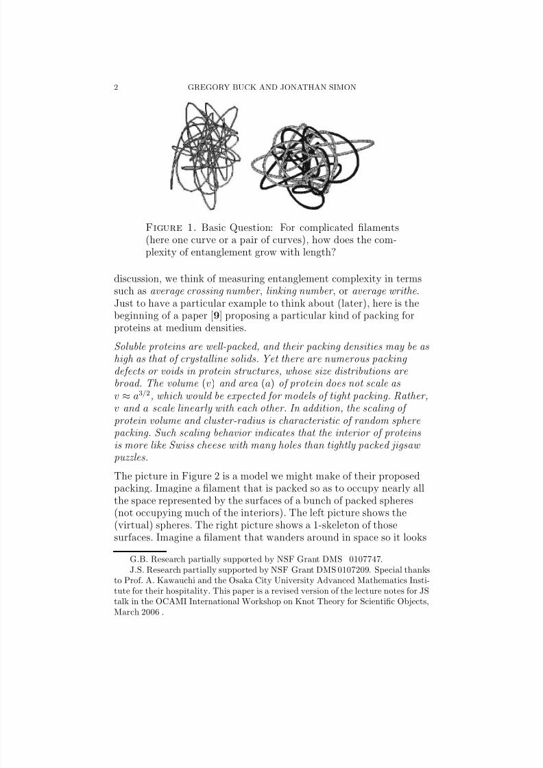
We are interested in the general problem of measuring the“entanglement” for filament systems, such as in Figure 1. Our goal isto describe how the topological/geometric complexity of theentanglement can be bounded, or even better estimated, if weunderstand how densely the filament is packed in space. In this

1



2 GREGORY BUCK AND JONATHAN SIMON

Figure 1. Basic Question: For complicated filaments(here one curve or a pair of curves), how does the com-plexity of entanglement grow with length?

discussion, we think of measuring entanglement complexity in termssuch as average crossing number , linking number , or average writhe.Just to have a particular example to think about (later), here is thebeginning of a paper [9] proposing a particular kind of packing forproteins at medium densities.

Soluble proteins are well-packed, and their packing densities may be ashigh as that of crystalline solids. Yet there are numerous packing defects or voids in protein structures, whose size distributions arebroad. The volume (v) and area (a) of protein does not scale asv

≈a3/2, which would be expected for models of tight packing. Rather,

v and a scale linearly with each other. In addition, the scaling of protein volume and cluster-radius is characteristic of random spherepacking. Such scaling behavior indicates that the interior of proteinsis more like Swiss cheese with many holes than tightly packed jigsaw puzzles.

The picture in Figure 2 is a model we might make of their proposedpacking. Imagine a filament that is packed so as to occupy nearly allthe space represented by the surfaces of a bunch of packed spheres(not occupying much of the interiors). The left picture shows the(virtual) spheres. The right picture shows a 1-skeleton of those

surfaces. Imagine a filament that wanders around in space so it looks

G.B. Research partially supported by NSF Grant DMS 0107747.J.S. Research partially supported by NSF Grant DMS 0107209. Special thanks

to Prof. A. Kawauchi and the Osaka City University Advanced Mathematics Insti-tute for their hospitality. This paper is a revised version of the lecture notes for JStalk in the OCAMI International Workshop on Knot Theory for Scientific Objects,March 2006 .



MODELS OF ENTANGLEMENT 3

approximately like that 1-skeleton. What is the topological

complexity of that filament?

Figure 2. What is the average crossing number of the1-complex that models protein filaments packed denselyalong spherical shells?

Our basic thesis is that in any filament system, there is acharacteristic rate of spatial packing: how much length is contained inhow much volume. And the expected growth rate of entanglement,relative to the length L of the filament, should be estimated first (inparticular, bounded) by a power of the filament length determinedfrom the packing rate. There are three basic “regimes” of packing:Linear, Laminar, and Globular. The bounds (which are “predictions”if the systems are “random”) for the associated growth rates of average crossing numbers are L1, Llog(L), and L4/3. When thegrowth rates differ from these, we can conclude that the filamentsystem involves some bias in how the filament is arranged within thegiven packing regime. In the protein example above, the packing is“laminar”, and we expect the average crossing number to be on theorder of Llog(L).There is another regime for packing that we can view as a theoreticalupper bound of density: ignore any physical thickness of the filamentsand allow an infinite length of string to be packed in a finite volume.In this “Infinite Density” regime, we see tangling on the order of L2.

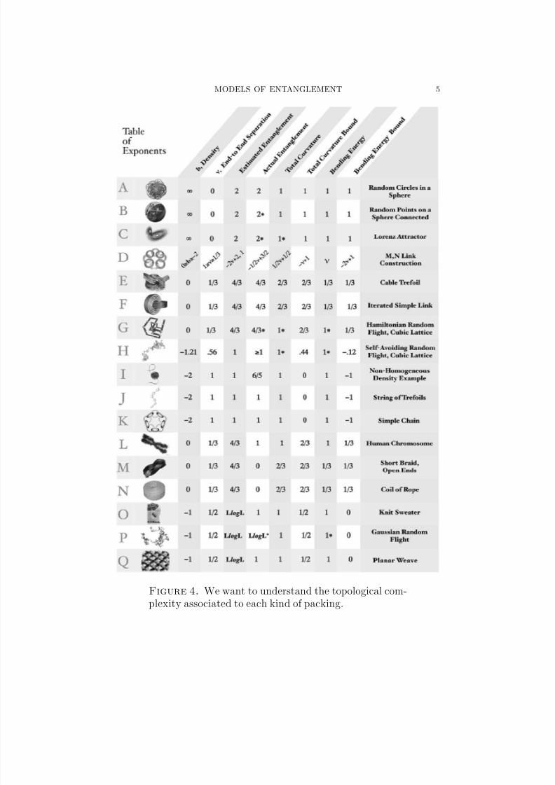
In Figure 3, we see a few of the many ways filaments can be packed.The chart in Figure 4 lists the geometry expectations/bounds forthese and other situations. Example (N), a neat coil of rope, is anextreme situation where the packing is spatially dense, yet so orderlythat there is essentially no tangling. On the other hand, the orderly




packing in Example (F) achieves the upper bound L4/3, which wouldalso be achieved by rope that is randomly arranged but tightly

packed in a space-filling way in a confined box.

Figure 3. There are many ways that filaments can be“packed” in space.




Figure 4. We want to understand the topological com-plexity associated to each kind of packing.




1.1. How to measure tangling? The topological knot or linktype seems intuitively to be the fundamental lower bound on how

much entanglement there is in some filament system. [We still canwonder about the question of defining how “tangled” is a given knottype: algebraic invariants? minimum crossing number? unknottingnumber?] But if a filament is an open string or complicated unknot(as in Figure 5), then there is no topological complexity even thoughthe filament(s) may appear to be very much tangled.

Figure 5. This curve is topologically trivial but, intu-itively, very tangled. (Example suggested for knot-energy

flows by M. Freedman, with some added twists)

So topological knot-type does not perfectly capture our intuitive ideaof entanglement. But it is a fundamental lower bound.

The other extreme of seemingly natural measures of entanglement is

the observed crossing-number: count the number of times a filamentcrosses over itself (or over another filament if we are studying severalinteracting strings). However, this number varies according to how welook at the curve. For example, the curve shown in Figure 6 has 42crossings as seen from one direction, and just 5 when seen fromanother.

Figure 6. This curve looks very different when seenfrom different directions




For this reason, people think in terms of averaging the number of crossings over all directions of viewing, the so-called average crossing

number . In the example of Figure 6, the average crossing number isapproximately 25.7.

1.2. Define ACN. The definition is made precise as an integralover the 2-sphere. For each direction vector v ∈ S 2, let c(K, v) denotethe number of crossings in the curve K as seen from direction v.Assuming K is [piecewise] smooth, this function is finite for all v

except perhaps for a set of measure zero in S 2. So the followingintegral makes sense:

Definition (Average Crossing Number).

ACN(K) =

1

4π v∈S2 c(K, v) dµS

2

.

The average crossing number for any particular curve of a given knottype is obviously an upper bound for the minimum crossing numberof the knot type; in fact, it is always strictly larger [7].We can to rewrite the ACN integral in a form that is useful forgetting bounds [4]. Define a map φ : K × K → S 2 by

φ(x, y) =x − y

|x − y| .

View this function as a parameterization of S 2 from the domainK

×K , and think of calculating the area of S 2 using this

parameterization. The function φ over-counts points of S 2: a pointv ∈ S 2 is hit q times precisely when c(K, v) = q. The weighted areaof S 2, divided by the area of S 2, is thus equal to the average crossingnumber. The integrand in the integral below is the Jacobian“stretching factor” (with respect to the area element dxdy onK × K ) for the given parameterization φ. We have

(1) ACN(K) =1

4π

x∈K

y∈K

| < Tx , Ty , x − y > ||x − y|3 dydx ,

where T x, T y are the unit tangents at x, y and < u, v,w > is the triplescalar product (u × v) · w of the three vectors u,v,w.

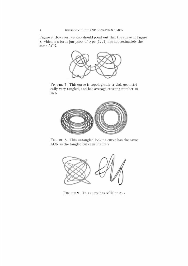
The “truth” of entanglement of a given curve lies somewhere betweenminimum crossing number of a topological knot-type and the averagecrossing number of the given curve. We are focusing in this paper oncalculating, or estimating, ACN. According to ACN, the curve inFigure 7 is approximately three times as tangled as the curve in




Figure 9. However, we also should point out that the curve in Figure8, which is a torus [un-]knot of type (12, 1) has approximately the

same ACN.

Figure 7. This curve is topologically trivial, geometri-cally very tangled, and has average crossing number

≈75.5

Figure 8. This untangled looking curve has the sameACN as the tangled curve in Figure 7

Figure 9. This curve has ACN ≃ 25.7




1.3. ACN is related to writhe and linking number. If wegive the curve(s) orientation(s), then each crossing has a sign, ±1.

For any projection, we can count the net total number of crossings,which might be positive, negative or zero. The average of this signedcrossing number, taken again over all spatial directions, is the averagewrithe for one curve, or the linking number for two. Thedouble-integral formula for ACN is just a slight adaptation of Gauss’sformula for the linking number of two (oriented) curves J, K :

Linking number(J, K ) =

1

4π

x∈J

y∈K

< T x , T y , x − y >

|x − y|3 dydx .

The only difference is that ACN uses the absolute value in thenumerator. Because ACN is so close conceptually to writhe andlinking number, and the integrals are so similar, it is not surprisingthat any method for bounding ACN probably also can be adapted togive a bound for writhe or linking number. Typically, the writhe(resp. linking number) is smaller in a fundamental way than ACN.We will discuss this more later.

1.4. Define Rope-Length . Suppose we are studying a situationinvolving some filament(s). If the total length of the filament(s) isvery small, then, intuitively, there cannot be very much tangling. So

the length of the filament(s) is an important parameter in controllingthe entanglement; call this L. We want to find bounds for thetangling of the form

ACN ≤ function of L .

This task seems hopeless as stated. We can make knots of arbitrarilyhigh complexity out of a tiny length of string: we just need to makethe string thin enough. So to model solid physical filaments, we needto keep track of the thickness of the filament, along with its length.

For any smooth curve K in 3-space R3, there is some ǫ > 0 such thatthe disks of radius ǫ centered at points of K , normal to K , are

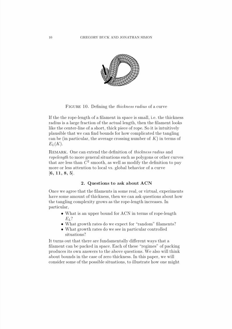
pairwise disjoint. Call such a radius “good”. In that case, the diskscombine to form a tubular neighborhood of K . Let R(K ), thethickness radius of K , be the supremum of all good ǫ. We define therope-length of K as

E L(K ) =arc length of K

R(K ).




Figure 10. Defining the thickness radius of a curve

If the the rope-length of a filament in space is small, i.e. the thicknessradius is a large fraction of the actual length, then the filament lookslike the center-line of a short, thick piece of rope. So it is intuitivelyplausible that we can find bounds for how complicated the tanglingcan be (in particular, the average crossing number of K ) in terms of E L(K ).

Remark. One can extend the definition of thickness radius andropelength to more general situations such as polygons or other curvesthat are less than C 2 smooth, as well as modify the definition to paymore or less attention to local vs. global behavior of a curve

[6, 11, 8, 5].

2. Questions to ask about ACN

Once we agree that the filaments in some real, or virtual, experimentshave some amount of thickness, then we can ask questions about howthe tangling complexity grows as the rope-length increases. Inparticular,

• What is an upper bound for ACN in terms of rope-lengthE L?

• What growth rates do we expect for “random” filaments?

• What growth rates do we see in particular controlledsituations?

It turns out that there are fundamentally different ways that afilament can be packed in space. Each of these “regimes” of packingproduces its own answers to the above questions. We also will thinkabout bounds in the case of zero thickness. In this paper, we willconsider some of the possible situations, to illustrate how one might




do these kinds of analyses. In particular, we will describe some simplemodels that convey the right intuition and clarify the questions one

should ask about real physical filament systems.In a real physical system, it might not be clear just what packingregime is involved. For example, if one is studying a collection of wiggly strands (e.g. some protein studies), can they best beunderstood as having zero thickness or some positive thickness? Dothe filaments pack densely so as to fill space or tend to escape andstretch out? Referring to table 4, example (G) illustrates positivethickness + dense packing; example (H) is positive thickness + avoidpacking; example (B) is zero thickness + forced “dense” spatialpacking; and example (P) is zero thickness + no forcing of packing.The Gaussian random flight in example (P) is perhaps the mostsubtle, since is exhibits similar behavior that seems to be a tippingpoint between globular and linear packing; it is somehow similar tothe orderly laminar packing illlustrated in example (Q). See the paper[3], and references therein (also earlier mentioned [9]), forquantitative discussions of competing models for actual proteinpacking and entangling.We will first define the several “regimes”, then describe the ACNbehavior in each. The discussions here emphasize intuitiveunderstanding and simple models. For more careful general proofs,see [2] or [12], and also see [1]. The papers [1, 12] contains detailedproofs for bounding ACN in terms of ropelength in the globularregime. It is easy to slightly modify the final section of [2] to get thedesired bounds for ACN in the other regimes: In that section of [2],

just multiply the “Illumination” bound by E L instead of multiplyingit by the total curvature.

3. Four regimes of packing

The same piece of “rope” can be packed in space in many ways. Inthe presence of filament thickness, there are three basic homogeneouspacking regimes: Linear, Laminar, and Globular, each having acharacteristic behavior of ACN. The fourth regime is filaments with

zero thickness, which can provide ultimate upper bounds.

3.1. Linear regime. The filament is packed in space in such away that the amount of filament within any fixed distance from apoint on the curve is roughly proportional to that distance. This isillustrated in Figure 11, which shows a long iterated connected sum of trefoil knots. In this situation, the amount of filament that lies




between spatial distance r and r + 1 relative to any given point isconstant (or, more realistically, is bounded between two constants).

Figure 11. Example of “linear regime” packing.

3.2. Laminar regime. See Figure 12. The filament is packed inspace in an essentially 2-dimensional way. The amount of filamentlength within any fixed distance r of a point is roughly proportionalto the area of a patch of surface of area r × r. The amount of filament

length that lies between distance r and r + 1 relative to any givenpoint is essentially proportional to r.

Figure 12. Example of laminar regime packing

3.3. Globular regime. See Figure 13. The filament is packed ina (nearly) space-filling way, so as to surround each of its points with apositive density of length per volume. That is, the amount of filamentlength that lies within a solid ball of radius r around any point isessentially proportional to r3, and the amount of filament lengthbetween distance r and r + 1 relative to any given point is

proportional to r2.

3.4. Zero-thickness, or infinite density, regime. In theexample shown in Figure 14, we generate paths by connectingconsecutive points (chosen randomly) on the boundary of a given ball.If the segments have no thickness, then we can keep on drawing sticksforever, with the path (generically) never crossing itself.




Figure 13. Example of globular regime packing

Figure 14. Infinitely dense packing in the zero-thickness regime

4. Answers: How does ACN grow with length in the various

regimes.

The case of zero thickness is perhaps easiest to understand. In ourexample above, where a polygonal curve is growing by successiverandom chords in a ball, each stick interacts strongly with all theothers, so the expected ACN should look like the square of thenumber, N , of sticks. Here is how we can quantify that intuition andget the desired estimate for ACN in terms of length.

Consider the original definition of ACN. How many crossings do weexpect to see from some direction? Once N is large, then lookingfrom any direction, we expect to see at least a certain fraction, p, of the sticks having projected length greater than, say, 1/2. Then wehave a variation of the Buffon needle problem: Two sticks of length≥ 1/2 contained in the unit disk have some probability q > 0 of crossing. So, for each pair of sticks, the probability of seeing them




cross from any given direction is > p2q. This gives

N 2 > ACN >N (N

−1)

2 p2q .

which says ACN is of order N 2. We can replace N by L, since thetotal length L of such a polygon is indeed proportional to N . Theaverage length of a random chord of the unit sphere is 4

3 , so L ≈ 43N .

The integral formula for ACN helps explain why the situation isdifferent for thick filaments. If the sticks have some finite thickness,and they are not allowed to overlap, then eventually we would have tomove to a larger ball to contain more sticks. In the integral formula(1) for ACN, the integrand decays with |x − y|2. So instead of having

ACN grow like L2

, we will see a lower power growth rate.Here are some answers that we will see in the subsequent discussion.For simplicity, assume that the world has been rescaled to have alwaysR(K )=1. This makes the rope-length = the actual length, L, of K .

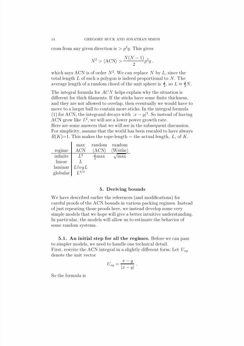
max random randomregime ACN ACN Writheinfinite L2 1

2max

√max

linear Llaminar LlogLglobular L4/3

5. Deriving bounds

We have described earlier the references (and modifications) forcareful proofs of the ACN bounds in various packing regimes. Insteadof just repeating those proofs here, we instead develop some verysimple models that we hope will give a better intuitive understanding.In particular, the models will allow us to estimate the behavior of some random systems.

5.1. An initial step for all the regimes. Before we can pass

to simpler models, we need to handle one technical detail.First, rewrite the ACN integral in a slightly different form: Let U xydenote the unit vector

U xy =x − y

|x − y| .

So the formula is




ACN(K) =

14π

x∈K

y∈K

| < T x , T y , U > ||x − y|2 dydx ,

The ACN integral includes two kinds of contributions, which arecontrolled differently. We distinguish between pairs of points (x, y)where x and y are close in the sense of arc-length along the curve(specifically where arc(x, y) ≤ π) and pairs (x, y) where x and y arefurther apart.When the point y is close to x, the denominator is close to 0, and oneeven has to worry if this improper integral converges. The key is thatwhen x and y are close, then T x and T y are close, so the cross product

T x × T y is small in size. At the same time, that cross product isperpendicular to the tangent vectors, and so nearly perpendicular toU . That makes the numerator approach zero as fast as thedenominator. If we are assuming the filaments have fixed thickness 1,this gives a bound on the curvature of the curves, which gives abound on how much U and T x can differ. That, in turn, gives auniform bound on the ACN integrand for the case where x and y areclose in arc-length along a curve. A careful analysis gives that forsmooth curves, the set of pairs

{(x, y) : arc(x, y) ≤ π} contributes ≤π3

8

(L) to ACN.

In the linear regime, the coefficient π3

8 would have to be added to

whatever coefficient we get for L coming from points that are furtherapart along the curve. In the other regimes, this contribution frompairs of nearby points gets eaten up by the rest of ACN, whichinvolves a higher power of L. (So again, one has to adjust thecoefficient of that power of L to consume the linear contribution.)We are left with the problem of understanding the (dominant) part of the ACN integral that comes from pairs (x, y) where arc(x, y) ≥ π.Another theorem about thickness of filaments [10] says that for suchpoints, the spatial distance |x − y| is ≥ 2. On the other hand, thenumerator in the ACN integral (5.1) is the triple scalar product of

three unit vectors; so it is ≤ 1. Thus the task of bounding ACNreduces to the task of bounding an integral of the form x,y

1

|x − y|2 dxdy ,

where x and y are points on the filament(s) where we knot the spatialdistance between them is bounded away from zero.




Note that if we are studying polygons (with thickness) instead of smooth curves, then ACN of consecutive sticks is 0. So polygon ACN

also reduces to understanding something that looks like 1/|x − y|2

.Just to keep the arithmetic as simple as possible, we will only assume|x − y| ≥ 1 rather than the available bound 2.

6. A very simple model

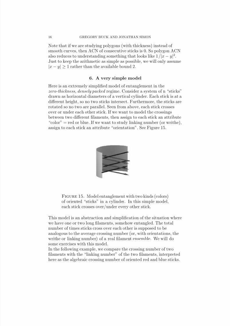
Here is an extremely simplified model of entanglement in thezero-thickness, densely packed regime. Consider a system of n “sticks”drawn as horizontal diameters of a vertical cylinder. Each stick is at adifferent height, so no two sticks intersect. Furthermore, the sticks arerotated so no two are parallel. Seen from above, each stick crosses

over or under each other stick. If we want to model the crossingsbetween two different filaments, then assign to each stick an attribute“color” = red or blue. If we want to study linking number (or writhe),assign to each stick an attribute “orientation”. See Figure 15.

Figure 15. Model entanglement with two kinds (colors)of oriented “sticks” in a cylinder. In this simple model,each stick crosses over/under every other stick.

This model is an abstraction and simplification of the situation wherewe have one or two long filaments, somehow entangled. The total

number of times sticks cross over each other is supposed to beanalogous to the average crossing number (or, with orientations, thewrithe or linking number) of a real filament ensemble. We will dosome exercises with this model.In the following example, we compare the crossing number of twofilaments with the “linking number” of the two filaments, interpretedhere as the algebraic crossing number of oriented red and blue sticks.




Although we are not including thickness at this point, this model is atemplate for studying that situation as well.

6.1. Crossing number vs. linking number in the

stack-of-thin-sticks model. We have N sticks; there are 2N waysto assign color red or blue to each stick. Of these, there are

N r

ways

to select r sticks to be red, with the rest blue. Since each red stick“interacts” with each blue stick in the sense that they cross (as seenfrom above), for each of the

N r

color assignment types, we see

(r)(N − r) crossings.Assuming the colors are assigned randomly, that is randomly witheach color assignment equally likely, we would like to know theaverage over all possible color assignments of the (different-color)crossing numbers. Let us denote this average as

C RB

. Combining

the above counts, we have

C RB =

N r=0

N r

(r)(N − r)

2N

=1

4N (N − 1) .

In particular, according to this model, the average number of crossingsof one filament vs. another is expected to be on the order of thesquare of the total length of the filaments and half the total crossingnumber of the (uncolored) system. This is an extremely naive model,

but as indicated in the example at the beginning of Section 4, webelieve it captures the essential behavior of more complicated models.Now consider what happens if we count the crossings withorientations. Each crossing gets a value, ±1 in the usual way.We have N sticks. There are 4N ways to assign colors andorientations to the sticks. Let us denote color “red” by the number+1 and “blue” by number −1, and let ci be the color assigned to sticki. Similarly, use xi = ±1 to denote the orientation of stick i. The, fora given assignment α of colors and orientations, the algebraic sum of the crossings, i.e. the “linking number” of the ensemble, is is

Lk(α) = 12

n−1 j=1

ni= j+1

xix j(ci − c j) .

Remark. The 12

is not to correct for duplication; it compensates for the fact that (ci − c j) = ±2.

Now consider all of the 4N possible labelings of N sticks. We get adistribution of values that we can analyze statistically. The analysis is




elementary (we thank statistics colleague R. Russo) but takes a bit of algebra. For each pair ( j,i), the number xix j(ci − c j) is ±2, with

equal probability. If the values for different pairs ( j,i) wereindependent of each other, then this would be simple coin-flipping.However, the values are not independent: for example, if the ( j,i)term and ( j,k) term are both zero [same colors], then so is the (k, i)term . Nevertheless, the distribution behaves a lot like coin flipping.The mean is, of course zero, and we can calculate the standarddeviation exactly .By symmetry, the mean is 0. Write out the square of Lk(α) explicitlyas an iterated sum. Simplify, using the fact that each of the numberbits is ±1. Use symmetry and a little induction to show that most of the terms add to zero; do a little more arithmetic to finish calculating

the variance σ2

.The distributions are (based on calculating exactly the distributionsfor several values of N) enough like normal distributions to justifyassuming that the standard deviation is a good approximation for themean absolute deviation, i.e. for the average magnitude of the linkingnumber. We obtain the following:For close packing of two filaments with 0 thickness,

• Total crossings =N (N −1)2 .

• C RB = (N )(N −1)4

.• Lk(α) = 0.

• Lk2(α)

= σ2 = (N )(N −1)

2.

• | Lk(α)| ≃ σ =

(N )(N −1)2 = 1√

2C RB.

The last statement is another instance of the well known phenomenonthat for many random processes, the average “drift” away from themean in n steps is on the order of

√n.

6.2. Crossing number in the stack-of-THICK-sticks

model. Here we model the Linear regime by assuming that the sticksin the previous model have some fixed amount of thickness, let it be 1.We can use the previous formulas for the crossing and linkingnumbers of the zero-thickness stick ensemble to give expressions forthe various kinds of tangling in the case of thick sticks. But now, thesummands in our estimate of ACN now have a damping-out effectproportional to 1/dist2, giving formulas as follows:




Lk(α) =1

2

N −1

j=1

N

i= j+1

xix j(ci − c j)

(i − j)2.

C RB(α) =1

2

N −1 j=1

N i= j+1

(ci − c j)

(i − j)2.

Writhe(α) =N −1 j=1

N i= j+1

xix j(i − j)2

.

ACN (α) =N −1 j=1

N i= j+1

1

(i − j)2.

The ACN estimate gives a bound for all the others, and is simple tocalculate, since it does not depend on the labels chosen for α.By collecting terms, we have

ACN (α) =N −1

k=1N −kk2

= (N )N −1

k=11k2

− N −1k=1

1k

≈ π2

6 N − ln(N ) .

The π2

6 N term dominates for large N, so we see that in the linearregime, with filaments having positive thickness, average crossingnumber is at most proportional to rope-length.

Remark. Our stack-of-sticks model allows all segments of thefilament(s) to interact with “full strength”, limited only by theirdistance apart. In actual ACN calculations, there also is the effect of relative angles between the sticks that would affect the numerator inthe ACN integral. So the behavior of the stack-of-sticks model is anupper bound for other situations in the linear regime. But so long asthe direction vectors for the filaments have a lot of freedom, weexpect the stack-of-sticks model to give the correct exponent for L,with appropriate corrections needed for the coefficients.




6.3. Model for the laminar regime. (See Figure 16)

Proposition. In the laminar regime, the bound on ACN (and theexpected behavior for random systems) is

ACN ≈ (L)(log L)

.

Proof. The amount of filament that lies within a given distanced from any one point x on the filament is proportional to d2. And theamount of filament that lies at distance d from x is proportional to d.Let D be the radius around x that is just large enough to enclose thefilament. So the length L (or number of sticks N ) is proportional toD.

Thus we can estimate ACN as

N Dk=1

d1

d2≈ N log(N ) .

Figure 16. “Sticks” model of the laminar regime

The proposed protein packing in Figure 2 does not look like Figure16. But it still is an example of the laminar regime. The amount of filament that lies within any fixed distance D of a typical point onthe filament is approximately proportional to D2.




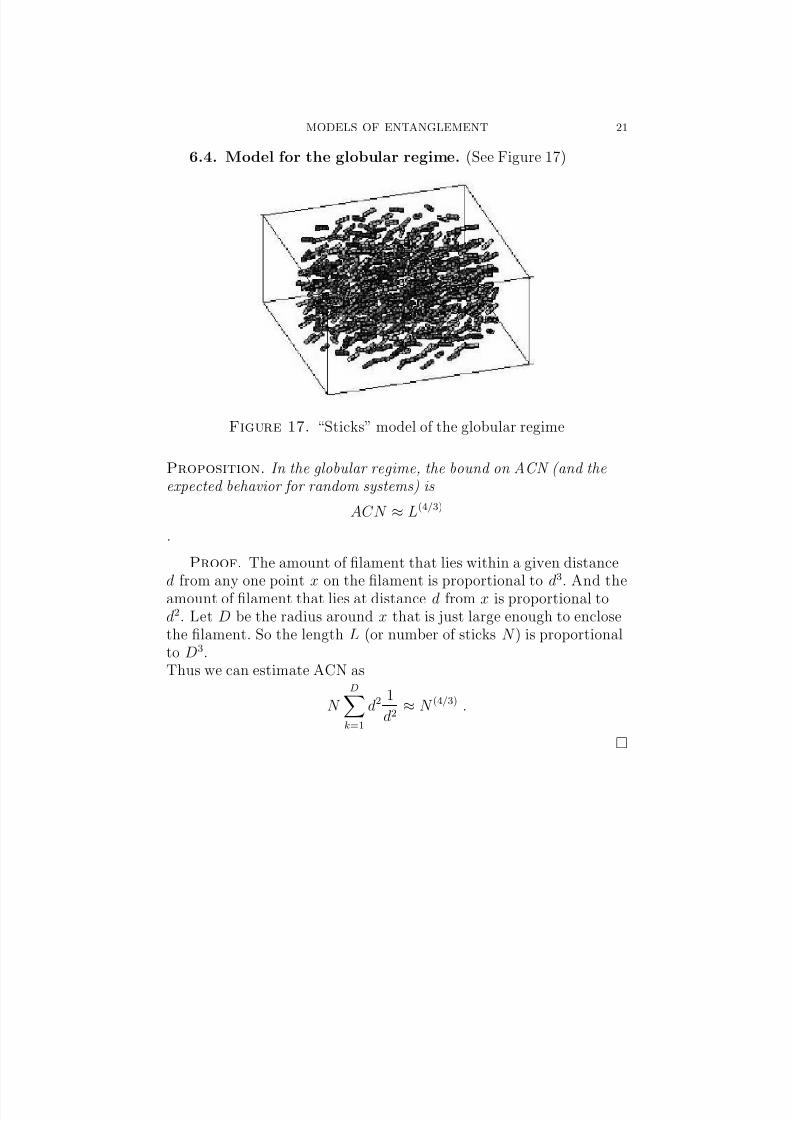
6.4. Model for the globular regime. (See Figure 17)

Figure 17. “Sticks” model of the globular regime

Proposition. In the globular regime, the bound on ACN (and theexpected behavior for random systems) is

ACN ≈ L(4/3)

.

Proof. The amount of filament that lies within a given distanced from any one point x on the filament is proportional to d3. And theamount of filament that lies at distance d from x is proportional tod2. Let D be the radius around x that is just large enough to enclosethe filament. So the length L (or number of sticks N ) is proportionalto D3.Thus we can estimate ACN as

N Dk=1

d21

d2≈ N (4/3) .




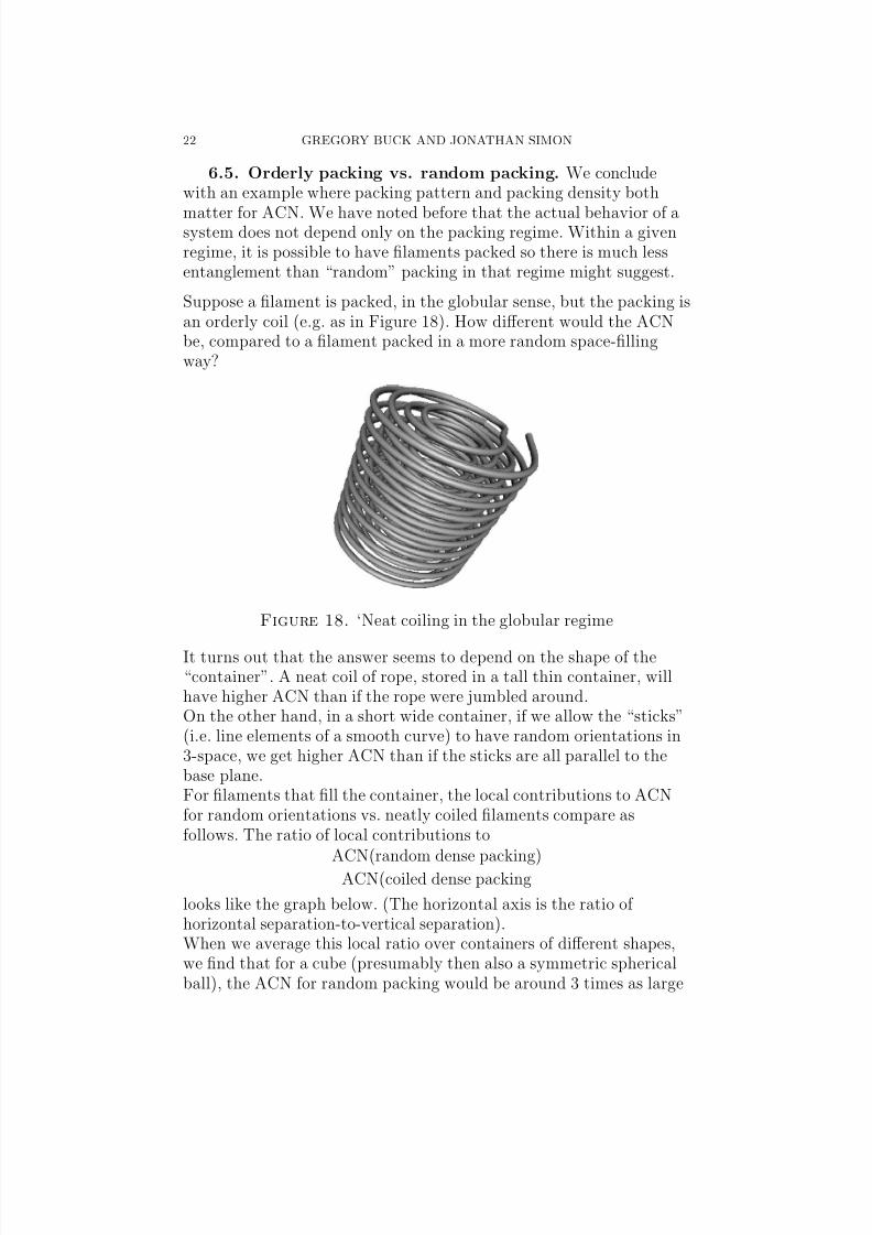
6.5. Orderly packing vs. random packing. We concludewith an example where packing pattern and packing density both

matter for ACN. We have noted before that the actual behavior of asystem does not depend only on the packing regime. Within a givenregime, it is possible to have filaments packed so there is much lessentanglement than “random” packing in that regime might suggest.

Suppose a filament is packed, in the globular sense, but the packing isan orderly coil (e.g. as in Figure 18). How different would the ACNbe, compared to a filament packed in a more random space-fillingway?

Figure 18. ‘Neat coiling in the globular regime

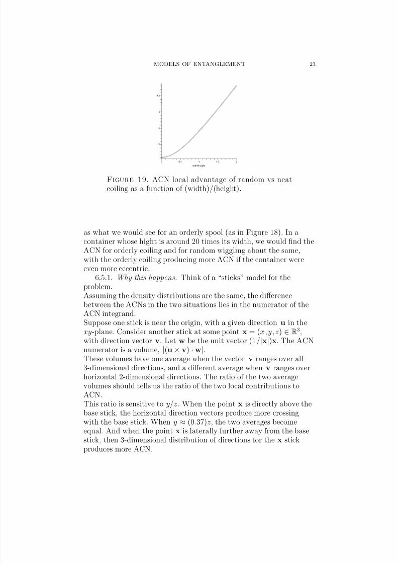
It turns out that the answer seems to depend on the shape of the“container”. A neat coil of rope, stored in a tall thin container, willhave higher ACN than if the rope were jumbled around.On the other hand, in a short wide container, if we allow the “sticks”(i.e. line elements of a smooth curve) to have random orientations in3-space, we get higher ACN than if the sticks are all parallel to thebase plane.For filaments that fill the container, the local contributions to ACNfor random orientations vs. neatly coiled filaments compare asfollows. The ratio of local contributions to

ACN(random dense packing)

ACN(coiled dense packing

looks like the graph below. (The horizontal axis is the ratio of horizontal separation-to-vertical separation).When we average this local ratio over containers of different shapes,we find that for a cube (presumably then also a symmetric sphericalball), the ACN for random packing would be around 3 times as large




Figure 19. ACN local advantage of random vs neatcoiling as a function of (width)/(height).

as what we would see for an orderly spool (as in Figure 18). In acontainer whose hight is around 20 times its width, we would find theACN for orderly coiling and for random wiggling about the same,with the orderly coiling producing more ACN if the container wereeven more eccentric.

6.5.1. Why this happens. Think of a “sticks” model for theproblem.

Assuming the density distributions are the same, the differencebetween the ACNs in the two situations lies in the numerator of theACN integrand.Suppose one stick is near the origin, with a given direction u in thexy-plane. Consider another stick at some point x = (x,y,z) ∈ R3,with direction vector v. Let w be the unit vector (1/|x|)x. The ACNnumerator is a volume, |(u × v) · w|.These volumes have one average when the vector v ranges over all3-dimensional directions, and a different average when v ranges overhorizontal 2-dimensional directions. The ratio of the two averagevolumes should tells us the ratio of the two local contributions to

ACN.This ratio is sensitive to y/z. When the point x is directly above thebase stick, the horizontal direction vectors produce more crossingwith the base stick. When y ≈ (0.37)z, the two averages becomeequal. And when the point x is laterally further away from the basestick, then 3-dimensional distribution of directions for the x stickproduces more ACN.




7. Additional Acknowledgements

Several figures and calculations of average crossing number were doneusing R. Scharein’s KnotPlot [13]. W. Hager helped confirm thebehavior of ACN in several situations. R. Russo provided a veryhelpful statistical argument.

References

[1] G. Buck and J. Simon, Thickness and crossing number of knots, Topologyand its Applications (91), 1999, 245–257.

[2] G. Buck and J. Simon, Total curvature and packing of knots, Topology andits Applications (154) 2007, 192–204.

[3] A. Dobay, J. Dubochet, A. Stasiak, and Y. Diao, Scaling of the average

crossing number in equilateral random walks, knots, and proteins, Physicaland Numerical Models in Knot Theory, Eds. J. Calvo, K.C. Millett, E.J.Rawdon, and A. Stasiak, World Scientific Publ. (Series on Knots andEverything vol. 36), 2005, 219–232.

[4] M. Freedman, Z.-X. He, and Z. Wang,On the M¨ obius energy of knots and

unknots, Annals of Math. (139), 1994, 1–50.[5] Y. Diao, C. Ernst, and E. J. Janse van Rensburg, Thicknesses of knots,

Math. Proc. Camb. Phil. Soc. (126), 1999, 293–310.[6] O. Gonzalez and J.H. Maddocks, Global curvature, thickness and the ideal

shapes of knots, Proceedings of the National Academy of Sciences, USA, 96(1999), 4769–4773.

[7] This proposition is attributed to N. Kuiper: Given a space curve K

representing a nontrivial knot type [K ], there is some direction from whichthe apparent crossing number of K is strictly larger than the minimum

crossing number of the knot-type.[8] R. Kusner and J. Sullivan, On distortion and thickness of knots, Topologyand Geometry in Polymer Science, Springer Verlag Publ., 1998, 67–78.

[9] J. Liang, J. Zhang and R. Chen, Statistical geometry of packing defects of

lattice chain polymer from enumeration and sequential Monte Carlo method ,Journal of Chemical Physics (117), 2002, 3511–3521.

[10] R. Litherland, J. Simon, O. Durumeric, and E. Rawdon, Thickness of knots,Topology and its Applications (91), 1999, 233–244.

[11] E. J. Rawdon, Approximating smooth thickness, J. Knot Theory and itsRamifications (9), 2000, 113–145.

[12] E. Rawdon and J. Simon, Mobius energy of thick knots, Topology and itsApplications (125) 2002, 97–109.

[13] R. Scharein, KnotPlot software system. See

http://www.pims.math.ca/knotplot/KnotPlot.html

G. Buck. Department of Mathematics, St. Anselm College, Manchester NH03102. [email protected]

J. Simon. Department of Mathematics, University of Iowa,Iowa City IA 52242 [email protected]

gregory buck and jonathan simon- models of entanglement

Documents