green’s theorem and gorenstein …jmiglior/ams-final.pdfgreen’s theorem and gorenstein sequences...
TRANSCRIPT
GREEN’S THEOREM AND GORENSTEIN SEQUENCES
JEAMAN AHN, JUAN C. MIGLIORE, AND YONG-SU SHIN
ABSTRACT. We study consequences, for a standard graded algebra, of extremal behavior in Green’s Hyper-plane Restriction Theorem. First, we extend his Theorem 4 from the case of a plane curve to the case ofa hypersurface in a linear space. Second, assuming a certain Lefschetz condition, we give a connection to ex-tremal behavior in Macaulay’s theorem. We apply these results to show that (1, 19, 17, 19, 1) is not a Gorensteinsequence, and as a result we classify the sequences of the form (1, a, a−2, a, 1) that are Gorenstein sequences.
CONTENTS
1. Introduction 12. Background 33. Relations between Green’s theorem and Macaulay’s theorem 54. Classification of Gorenstein sequences of the form (1, r, r − 2, r, 1) 155. Acknowledgements 22References 22
1. INTRODUCTION
In the study of Hilbert functions of standard graded algebras, Macaulay’s theorem [21] and Green’stheorem [17] stand out as being of fundamental importance both on a theoretical level and from the pointof view of applications. Macaulay’s theorem regulates the possible growth of the Hilbert function from onedegree to the next. It is a stunning fact that strong geometric consequences arise whenever the maximumpossible growth allowed by this theorem is achieved [16], [8], [2], or even when the maximum is almostachieved [11]. Green’s theorem regulates the possible Hilbert functions of the restriction modulo a generallinear form. It is a less-studied question to ask what happens if the maximum possible Hilbert functionoccurs for this restriction, although already Green gave some intriguing results [17], [9] in his so-called“Theorem 3" and “Theorem 4," and some results in this direction can also be found in [1]. To our knowledge,the connections between these two kinds of extremal behavior have not previously been studied.
One area where both Macaulay’s theorem and Green’s theorem have been applied very profitably is theproblem of classifying the Hilbert functions of Artinian Gorenstein algebras (i.e. of finding all possibleGorenstein sequences). Of course this problem is probably intractable in full generality. However, manypapers have been written on the subject, and we cannot begin to list them all here. Even the special caseof socle degree 4 (i.e. Gorenstein sequences of the form (1, a, b, a, 1)) has been carefully studied (see forinstance [30], [27], [3], [9], [28], [5]), but a full classification remains open.
Given the ubiquity of Gorenstein rings [6], the problem of classifying the possible Gorenstein sequencesis of intrinsic interest. However, the unimodality question also has a strong motivation coming from geom-etry and combinatorics. As noted in [26], the Stanley-Reisner ring of the boundary complex of a convexpolytope is a reduced Gorenstein ring, and the g-theorem classifies their h-vectors as being the so-calledSI-sequences. These sequences are defined as being unimodal symmetric sequences such that the first dif-ference of the “first half” is an O-sequence. It was shown in [25] that over a field of characteristic zero, every
2010 Mathematics Subject Classification. Primary:13D40; Secondary:13H10, 14C20.1

SI-sequence is even the h-vector of a simplicial polytope with whose Stanley-Reisner ring has maximal Bettinumbers among simplicial polytopes with the given h-vector. The SI-property is proven (following Stanley)by proving that the weak Lefschetz property (WLP) holds for that ring. It is an open question whether thesame result holds for simplicial spheres; this would follow from an affirmative answer to Question 1.4 of[25], namely whether every reduced, arithmetically Gorenstein subscheme of projective space possesses theWLP. A negative answer would arise by producing an artinian Gorenstein algebra that “lifts” to a reducedset of points but does not have a unimodal h-vector. Hence we are motivated to study artinian Gorensteinalgebras whose Hilbert function is not unimodal.
In this paper we make progress on both problems. First, we study some consequences of extremality forGreen’s theorem, including an analysis of a situation where we have an equivalence between this extremalityand that for Macaulay’s theorem. Next we apply this work to produce new results on Gorenstein sequencesof socle degree 4.
More precisely, after recalling known facts in section 2, our main goal in section 3 is to find new conse-quences of extremal behavior in Green’s theorem. We recall Green’s Theorem 4 and we first prove a directgeneralization in Theorem 3.2, passing from Green’s case of a plane curve to the case of a hypersurface in alinear subspace. Our main result in this section is Theorem 3.5, which gives a connection, under certain as-sumptions, between extremal behavior for Green’s theorem and extremal behavior for Macaulay’s theorem.Because of this connection, Gotzmann’s theorem applies as it did in the paper [8] to give strong geomet-ric consequences, which we explore in Corollary 3.7. We also show that Green’s theorem is “sequentiallysharp" in Corollary 3.11.
An important feature of our work is a study of the geometric and algebraic consequences resulting fromcertain assumptions on the end of the binomial expansion of some term of the Hilbert function, if Green’stheorem is sharp in that degree. See for instance the conditions e ≥ 2 of Theorem 3.5 or ae > e of Corollary3.7 (iv). It was pointed out to us by the referee that this feature could be a motivation for further studies onthis topic.
We apply our new results on Green’s theorem in Section 4 to show that the sequence (1, 19, 17, 19, 1) isnot Gorenstein (Theorem 4.1). Our proof brings together a number of different techniques. The result is themain ingredient for our Corollary 4.3, which completes the classification of the socle degree 4 Gorensteinsequences with a − b = 2 (with the notation introduced above) by proving that the sequence is Gorensteinif and only if a ≥ 20.
Theorem 3.5 makes a certain numerical assumption as well as a certain Lefschetz assumption in order toconclude that the two different kinds of extremal behavior are equivalent. This gives a new illustration of theimportance of the so-called Lefschetz properties, which have been studied very extensively in the last twodecades, especially the Weak Lefschetz Property (WLP) and the Strong Lefschetz property (SLP). However,it is worth noting here that our Lefschetz assumption is much milder than WLP. Instead, we only assume thatmultiplication on our algebra by a general linear form is injective in just one degree. Interestingly, there aretwo different degrees where such an assumption leads to the equivalence mentioned above. This Lefschetz(injectivity) assumption can be phrased in more than one way, as shown in Lemma 3.4. It also leads to asurprisingly simple but useful result, Lemma 3.12, which forces the existence of a socle element in a specificdegree. It is a small improvement of [23, Proposition 2.1 (b)], although our proof is completely different. Itprovides a very simple way to rule out cases, via the existence of socle elements, in our study of Gorensteinsequences in the last section.
Finally, we make a remark on the characteristic. In their paper [9], M. Boij and F. Zanello (and M. Greenin the appendix) make a careful study of its role. They note that Green’s theorem and Macaulay’s theoremare true independently of the characteristic. However, Green’s Theorem 3 (see Corollary 3.3 below) requireschar k 6= 2, and Green’s Theorem 4 (see Theorem 3.1) requires char k = 0 (although they point out that thecharacteristic can simply be “large enough" in a sense that they make precise). Since our Theorem 3.2 usesGreen’s Theorem 4 for the induction, we also assume characteristic zero there, and hence the same is true
2

of Corollary 3.3. And because we use this result in one place in the proof of Theorem 4.1, we also assume itthere. However, the main results of Section 3 are independent of the characteristic.
2. BACKGROUND
Let k be an infinite field and let R = k[x0, . . . , xn] be the homogeneous polynomial ring. Let A = R/Ibe a standard graded Artinian k-algebra, i.e. an Artinian graded quotient of R. The Hilbert function of A isthe function on the natural numbers defined by H(A, d) = dimk[A]i. SinceA is Artinian, we often representthis function by the h-vector (1 = h0, h1, . . . , he) with he > 0, where hi = H(A, i). The integer e is calledthe socle degree of A.
Let L /∈ I be a linear form in R. We have the graded exact sequence
(2.1) 0→ R/(I : L)(−1)→ R/I → R/(I, L)→ 0.
Notation 2.1. Throughout this paper we shall adopt the following:
hi = dimk[A]ibi = dimk[R/(I : L)]i`i = dimk[R/(I, L)]i.
The following is well known, and the first part follows from the above sequence.
Lemma 2.2 ([31]). Let A = R/I be a graded Artinian algebra, and let L /∈ I be a linear form of R. Thenwe have
H := (h0, h1, . . . , he) = (1, b0 + `1, . . . , be−2 + `e−1, be−1 + `e).
Furthermore, if A is Gorenstein then so is R/(I : L), and be−1 = he = 1:
H := (h0, h1, . . . , he−1, he = 1) = (1, b0 + `1, . . . , be−2 + `e−1, be−1 = 1)
In this paper A will always be Gorenstein, and we will often use the following notation.
Notation 2.3. With notation as in Lemma 2.2, we shall simply call the following diagram
h0 h1 h2 · · · he−1 heb0 b1 · · · be−2 be−1
`0 `1 `2 · · · `e−1 `e
the decomposition of the Hilbert function H.
Definition 2.4. Let r and i be positive integers. The i-binomial expansion of r is
r(i) =
(rii
)+
(ri−1
i− 1
)+ ...+
(rjj
),
where ri > ri−1 > ... > rj ≥ j ≥ 1. Such an expansion always exists and is unique (see, e.g., [10], Lemma4.2.6). Following [10], we define, for any integers a and b,
r(i)|ba =
(ri + b
i+ a
)+
(ri−1 + b
i− 1 + a
)+ ...+
(rj + b
j + a
),
where we set(mc
)= 0 whenever m < c or c < 0.
We now present the theorems of Macaulay, Green and Gotzmann. Nice treatments of these theorems canbe found in [10], Sections 4.2 and 4.3, and in [20], section 5.5.C.
Theorem 2.5 ([17], [21]). Let hd be the entry of degree d of the Hilbert function of R/I and let `d be thedegree d entry of the Hilbert function of R/(I, L), where L is a general linear form of R. Then, we have thefollowing inequalities.
(a) Macaulay’s Theorem: hd+1 ≤((hd)(d)
)|+1+1.
3

(b) Green’s Hyperplane Restriction Theorem (Theorem 1): `d ≤((hd)(d)
)|−1
0.
Definition 2.6. Let M be a finitely generated graded R-module with minimal free resolution
0→ Fm → · · · → F1 → F0 →M → 0
whereFp = ⊕jR(−apj ).
Then M is d-regular if apj − p ≤ d for all p, j. The regularity of M , denoted reg(M), is the smallest dfor which M is d-regular; thus the regularity equals max{apj − p}. Alternatively, the regularity of M is thelargest q for which TorRp (M,R/m)p+q 6= 0 for some p. Note that if M = R/I for a homogeneous ideal Ithen reg(R/I) = reg(I)− 1.
Alternatively, if we writeFi :=
⊕rit=0R(−(i+ 1 + t))βi,i+1+t
then the numbers {βi,j} for 1 ≤ i ≤ m are called the ith graded Betti numbers of the ideal I . A tablecollecting the graded Betti numbers (see for instance part (ii) of Theorem 4.1) is called a Betti table.
Theorem 2.7 ([16], Gotzmann’s Persistence Theorem). Let I be a homogeneous ideal generated in degrees≤ d+ 1. If in Macaulay’s estimate,
hd+1 = ((hd)(d))|+1+1,
then I is d-regular andht+1 = ((ht)(t))|+1
+1
for all t ≥ d.
Definition 2.8. Let R/I be a graded Artinian ring such that [R/I]t 6= 0 and [R/I]t+1 = 0. The socle ofR/I is defined by
Soc(R/I) := AnnR/I(m) = {a ∈ R/I | a ·m = 0},and an element a in Soc(R/I) is called a socle element of R/I . If Soc(R/I) = [R/I]t then R/I is called alevel Artinian algebra.
Let R/I be a level Artinian algebra, and J be an ideal of R. An Artinian ring R/(I + J) is called a levelquotient of R/I if R/(I + J) is also level.
The following result, with a small change in notation, is [33], Theorem 3.5.
Lemma 2.9. Let H = (h0, . . . , hd−1, hd, hd+1, . . . , he) be an h-vector of an Artinian ring R/J . Supposethat, for some d > 0, there is a positive integer ε > 0 such that
hd−1 = (hd)(d)|−1−1 + ε and hd+1 = (hd)(d)|+1
+1.
Then the ring R/J has socle of dimension ε in degree d− 1. Consequently, if R/J has the graded minimalfree resolution as in Definition 2.6, then
βr,r+d−1(R/J) = ε.
Remark 2.10. As noted in [33] Example 3.6, Lemma 2.9 slightly generalizes Theorem 3.4 in [15] (see also[12]). For example, consider an Artinian ring R/I with an h-vector
H = (1, 18, 16, 18, 28).
Note that there is no positive integer h2 such that
(h2)(2)|+1+1 = h3,
and thus we cannot apply Theorem 3.4 in [15] to show that R/J has a socle element in degree 3.However, by Theorem 2.5 (a), R/I has maximal growth in degree 3. Moreover, since
(18)(3)|−1−1 = 10,
we get that R/I has a 6-dimensional socle in degree 3.4

Proposition 2.11 ([7]). I is m-saturated if and only if, for a general linear form L ∈ R, (I : L)d = Id forevery d ≥ m.
The following result is well known and follows from standard methods.
Theorem 2.12 ([24]). If (1, n, a, n, 1) is a Gorenstein h-vector then so are (1, n, b, n, 1) for each a ≤ b ≤(r+1
2
)and (1, n+ 1, a+ 1, n+ 1, 1).
We also need the following decomposition theorem from [28], originally shown in [15], Lemma 2.8 andTheorem 2.10.
Theorem 2.13. Let h = (1, h1, . . . , he = t) be the h-vector of a level algebra A of type t, and let h′ =(1, h′1, . . . , h
′e = t− 1) be the h-vector of any level quotient of A of type t− 1 and the same socle degree, e.
Then the reverse of the difference of h and h′, namely (1, he−1−h′e−1, he−2−h′e−2, . . . ), is an O-sequence.
3. RELATIONS BETWEEN GREEN’S THEOREM AND MACAULAY’S THEOREM
Several papers have studied geometric and algebraic consequences for a standard graded algebra when itsHilbert function achieves the maximal growth in some degree allowed by Macaulay’s theorem (Theorem 2.5(a)). See for instance [16], [13] [8], [2], [11]. Not as much work has been done, to our knowledge, exploringthe consequences of extremal behavior of the Hilbert function under Green’s theorem (Theorem 2.5 (b))other than Green’s Theorem 3 and Theorem 4 (see [17], [9]). In this section we generalize Green’s Theorem4, and we give some results that connect the two kinds of extremality.
Throughout this section and the next we will use binomial expansions, and we refer to Definition 2.4 forthe conditions on the various integers. We first recall Green’s Theorem 4. Recall also from Notation 2.1 that`d = dimk[R/(I, L)]d. Observe that the indicated restriction is extremal according to Green’s theorem.
Theorem 3.1 (Green’s Theorem 4). Let I ⊂ R = k[x0, . . . , xn] be a homogeneous ideal. Assume thatchar k = 0 and suppose that, for some integers m and d, 1 ≤ m ≤ d, we have the binomial expansion
hd = md+ 1−(m− 1
2
)=
(d+ 1
d
)+
(d
d− 1
)+ · · ·+
(d− (m− 2)
d− (m− 1)
)and `d = m = (hd)|−1
0. Then in degree d, I is the ideal of a plane curve of degree m. That is,
[I]d = 〈L0, L1, L2, . . . , Ln−3〉+ F · [R]d−m
where L0, L1, L2, . . . , Ln−3 are linearly independent linear forms and F is a form of degree m.
This result can be generalized as follows.
Theorem 3.2. Let I ⊂ R = k[x0, . . . , xn] be a homogeneous ideal. Assume that char k = 0 and that forsome degree d and integers c and k we have the binomial expansion
hd =
(d+ c
d
)+ · · ·+
(d+ c− kd− k
)and `d = (hd)|−1
0.
Then there is a hypersurface F of degree k + 1 in a (c+ 1)-dimensional linear space Λ ⊂ P(R1) such that
[I]d = [IΛ + IF ]d = 〈L0, L1, . . . , Ln−c−2, F 〉d.
Proof. The proof is by induction on c. Let L and L′ be general linear forms. The case c = 1 is Theorem 3.1(Green’s Theorem 4), so we will assume c ≥ 2. Consider the diagram
5

(3.1)
0 0 0↓ ↓ ↓
[R/((I : L) : L′)]d−2 [R/(I : L′)]d−1 [R/((I, L) : L′)]d−1
↓×L′ ↓×L′ ↓×L′
0 → [R/(I : L)]d−1×L−→ [R/I]d → [R/(I, L)]d → 0
↓ ↓ ↓[R/((I : L), L′)]d−1 [R/(I, L′)]d [R/(I, L, L′)]d
↓ ↓ ↓0 0 0
The assumptions give the dimensions in the middle row of (3.1) of the second and third vector spaces:
(3.2)
hd = dim[R/I]d
=
(d+ c
d
)+ · · ·+
(d+ c− kd− k
)=
(d+ c
c
)+ · · ·+
(d+ c− k
c
)=
(d+ c+ 1
c+ 1
)−(d+ c− kc+ 1
),
and
(3.3)
dim[R/(I, L)]d =
(d+ c− 1
d
)+ · · ·+
(d+ c− k − 1
d− k
)=
(d+ c− 1
c− 1
)+ · · ·+
(d+ c− k − 1
c− 1
)=
(d+ c
c
)−(d+ c− k − 1
c
).
Then a calculation gives
dim[R/(I : L)]d−1 =
(d+ c− 1
d− 1
)+ · · ·+
(d+ c− k − 1
d− k − 1
)=
(d+ c
c+ 1
)−(d+ c− k − 1
c+ 1
).
Looking at the first column of (3.1), Green’s Theorem 1 then gives
dim[R/((I : L), L′)]d−1 ≤(d+ c− 2
d− 1
)+ · · ·+
(d+ c− k − 2
d− k − 1
)=
(d+ c− 1
c
)−(d+ c− k − 2
c
).
Green’s Theorem 1 applied to the third column of (3.1), thanks to our assumptions, gives
dim[R/(I, L, L′)]d ≤ (hd)|−20 =
(d+ c− 1
c− 1
)−(d+ c− k − 2
c− 1
).
Since((I, L′) : L) ⊇ ((I : L), L′),
we obtain
dim[R/((I, L′) : L)]d−1 ≤(d+ c− 1
c
)−(d+ c− k − 2
c
)and the sequence
0→ [R/((I, L′) : L)]d−1 → [R/(I, L′)]d → [R/(I, L, L′)]d → 06
gives(d+ c
c
)−(d+ c− k − 1
c
)= dim[R/(I, L′)]d
= dim[R/((I, L′) : L)]d−1 + dim[R/(I, L, L′)]d
≤[(d+ c− 1
c
)−(d+ c− k − 2
c
)]+
[(d+ c− 1
c− 1
)−(d+ c− k − 2
c− 1
)]=
(d+ c
c
)−(d+ c− k − 1
c
).
We conclude
dim[R/((I, L′) : L)]d−1 =
(d+ c− 1
c
)−(d+ c− k − 2
c
)and
(3.4)dim[R/(I, L, L′)]d =
(d+ c− 1
c− 1
)−(d+ c− k − 2
c− 1
)= (hd) |−2
0 .
Now combining (3.3) and (3.4), we see that the ideal (I, L) satisfies the inductive hypothesis for c − 1. Byinduction, then, (I, L) is the saturated ideal of some hypersurface, F ′, of degree k + 1 in a linear space Λ′
of dimension c, which is contained in the hyperplane defined by L.Let Y be the scheme in Pn defined by I (which a priori is not necessarily saturated in degree d). Then
F ′ is the hyperplane section of Y cut out by the general hyperplane defined by L. Since F ′ is arithmeticallyCohen-Macaulay, Y must be the union of a hypersurface of degree k+1 in some linear space Λ of dimensionc+ 1, and possibly a finite set of points. But (3.2) is the Hilbert function of the hypersurface of degree k+ 1alone (in the linear space Λ). Thus [I]d is the degree d component of the saturated ideal of Y = F , asclaimed. �
This result implies Green’s Theorem 3, at least with the stronger assumption on the characteristic inTheorem 3.2. (In the correction of Green’s Theorem 3 given in the appendix of [9], the assumption on thecharacteristic is only that char k 6= 2.)
Corollary 3.3 (Green’s Theorem 3). In the penultimate line in the statement of Theorem 3.2, if k = 0 then[I]d is the degree d component of the saturated ideal of a linear space of dimension c.
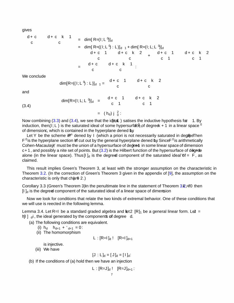
Now we look for conditions that relate the two kinds of extremal behavior. One of these conditions thatwe will use is reflected in the following lemma.
Lemma 3.4. Let R/I be a standard graded algebra and let L ∈ [R]1 be a general linear form. Let J =〈[I]≤d〉, the ideal generated by the components of I of degree ≤ d.
(a) The following conditions are equivalent.(i) hd − hd+1 + `d+1 = 0.
(ii) The homomorphism×L : [R/I]d → [R/I]d+1
is injective.(iii) We have
[J : L]d = [J ]d = [I]d.
(b) If the conditions of (a) hold then we have an injection
×L : [R/J ]d → [R/J ]d+1.
7

Proof. Part (a) is immediate from the exact sequence
0→ [(I : L)/I]d → [R/I]d×L−→ [R/I]d+1 → [R/(I, L)]d+1 → 0.
For part (b), notice that [I]d = [J ]d and [J ]d+1 ⊆ [I]d+1. Consider the commutative diagram
0↓
0 → [R/J ]d → [R/I]d → 0↓ ↓ ×L ↓ ×L
0 → [I/J ]d+1 → [R/J ]d+1 → [R/I]d+1 → 0
Then the result follows from the Snake Lemma. �
In the following theorem, we see the effect of two different assumptions on the multiplication by a generallinear form on R/I . This result is independent of the characteristic.
Theorem 3.5. Let I ⊂ R = k[x0, x1, . . . , xn] be a homogeneous ideal. Let L be a general linear form. LetJ = 〈[I]≤d〉, the ideal generated by the components of I of degree ≤ d. Assume that for some integer d wehave the binomial expansion
hd = dimk[R/I]d =
(add
)+
(ad−1
d− 1
)+ · · ·+
(aee
), where e ≥ 2.
(a) Assume that the multiplication ×L : [R/I]d → [R/I]d+1 is injective. Then the following conditionsare equivalent:
(i) dim[R/(I, L)]d = (hd)|−10 (i.e. Green’s Theorem 1 is sharp for R/I in degree d);
(ii) The Hilbert function of R/(I : L) has maximal growth (i.e. Macaulay’s theorem is sharp) fromdegree d− 1 to degree d;
(iii) The Hilbert function ofR/(J : L) has maximal growth (i.e. Macaulay’s theorem is sharp) fromdegree d− 1 to degree d.
(iv) The Hilbert function of R/J has maximal growth (i.e. Macaulay’s theorem is sharp) from de-gree d to degree d+ 1;
(b) Assume that the multiplication ×L : [R/I]d−1 → [R/I]d is injective. Then the following conditionsare equivalent:(i) dim[R/(I, L)]d = (hd)|−1
0 (i.e. Green’s Theorem 1 is sharp for R/I in degree d);(ii) The Hilbert function ofR/I has maximal growth (i.e. Macaulay’s theorem is sharp) from degree
d− 1 to degree d;(iii) The Hilbert function ofR/(J : L) has maximal growth (i.e. Macaulay’s theorem is sharp) from
degree d− 1 to degree d.
Proof. Notice that [I]t = [J ]t for all t ≤ d, but we only have [J ]d+1 ⊆ [I]d+1. We first prove (a). By thedefinition of J , Green’s theorem is sharp for R/I in degree d if and only if it is sharp for R/J in degree d.Note that by Lemma 3.4, the injectivity assumption for (a) implies the corresponding injectivity for R/J aswell. Thanks to the exact sequences
0→ [(J : L)/J ]d → [R/J ]d×L−→ [R/J ]d+1 → [R/(J, L)]d+1 → 0
and0→ [(I : L)/I]d → [R/I]d
×L−→ [R/I]d+1 → [R/(I, L)]d+1 → 0
we obtain[J : L]d = [J ]d = [I]d = [I : L]d.
8

Consider the exact sequence
(3.5) 0→ [R/(I : L)]d−1×L−→ [R/I]d → [R/(I, L)]d → 0.
We are given the value of the second vector space in (3.5):
(3.6)hd = dim[R/I]d
=
(add
)+ · · ·+
(aee
).
We also know that
(3.7) (hd)|−10 =
(ad − 1
d
)+ · · ·+
(ae − 1
e
).
It is worth noting that we are allowing the case ae = e, in which case the last binomial coefficient (andpossibly others) in (3.7) becomes zero. A simple calculation gives
hd − (hd)|−10 =
(ad − 1
d− 1
)+ · · ·+
(ae − 1
e− 1
).
The exactness of (3.5) then gives that Green’s theorem is sharp in degree d if and only if
dim[R/(I : L)]d−1 =
(ad − 1
d− 1
)+ · · ·+
(ae − 1
e− 1
).
Since e ≥ 2, this is the (d−1)-binomial expansion for dim[R/(I : L)]d−1. Since [I]d = [I : L]d, the Hilbertfunction of R/(I : L) has maximal growth from degree d− 1 to degree d if and only if Green’s Theorem 1is sharp for R/I in degree d, proving the equivalence of (i) and (ii). The above equalities also immediatelygive (iii).
For part (a) it remains to prove the equivalence of (iv) to the other three conditions. Since J ⊂ (J : L) and[J : L]d = [J ]d, it is clear that (iii) implies (iv). Now we will show that (iv) implies (i). Assume thatR/J hasmaximal growth from degree d to degree d + 1. By the Gotzmann persistence theorem, R/J has maximalgrowth for all degrees greater than or equal to d, and J is k-regular for each k ≥ d. So J is k-saturated foreach k ≥ d, and there is a scheme X ⊂ Pn such that
Jk = [IX]k for each k ≥ d.
Define
M(X) = min{t | H(R/(IX, L), k) = (H(R/IX, k))(k) |−10 for each k ≥ t}, and
G(X) = min{t | H(R/IX, k + 1) = (H(R/IX, k))(k) |+1+1 for each k ≥ t}.
It follows from Proposition 3.1 in [1] that M(X) ≤ G(X) . So, our assumption implies that
M(X) ≤ G(X) ≤ d,
which meansdimk[R/(I, L)]d = dimk[R/(J, L)]d
= dimk[R/(IX, L)]d= (H(R/IX, d))(d) |−1
0 (since M(X) ≤ d)
= (H(R/J, d))(d) |−10
= (hd)(d) |−10 .
This concludes the proof of (a).We now assume the injectivity given in (b). Then we have
[J : L]d−1 = [J ]d−1 = [I]d−1 = [I : L]d−1 and [J ]d = [I]d.9
These equalities and the same calculation as in (a) give that (i) is equivalent to (ii). To see that (ii) implies(iii), suppose that the Hilbert function of R/J (equivalently R/I) has maximal growth from degree d− 1 todegree d. By Gotzmann’s theorem, the ideal J is (d−1)-regular (and hence (d−1)-saturated). This impliesthat
(J : L)k = Jk for all k ≥ d− 1.
Hence, the Hilbert function of R/(J : L) has maximal growth from degree d− 1 to degree d.Finally we prove that (iii) implies (i). For convenience, we use a small variation on the notation in Notation
2.1:
• hd = dim[R/J ]d = dim[R/I]d;• bd = dim[R/(J : L)]d;• `d = dim[R/(J, L)]d = dim[R/(I, L)]d;
Suppose that
(bd−1)(d−1) |+1+1= bd.
This implies that (J : L) has no generators of degree d. So, we have
Jd ⊂ (J : L)d = m(J : L)d−1 = m(J)d−1 ⊂ Jd,
where m is the maximal ideal of R. This means that
Jd = (J : L)d,
and thus
bd−1 = hd−1 and bd = hd.
By the assumption that
(bd−1)(d−1) |+1+1= bd,
we have that(bd−1)(d−1) |+1
+1 = (hd−1)(d−1) |+1+1
= [(hd − `d)](d−1)|+1+1
≥[hd − ((hd)(d)) |−1
0
](d−1)
|+1+1
= hd (since e ≥ 2)= bd= (bd−1)(d−1) |+1
+1 .
Since the function (−) |+1+1 is strictly increasing, we see that hd − `d = hd − (hd)(d) |−1
0, and thus
`d = (hd)(d) |−10,
as we wished. �
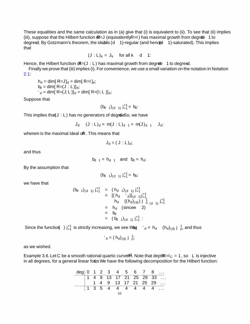
Example 3.6. Let C be a smooth rational quartic curve in P3. Note that depth R/IC = 1, so×L is injectivein all degrees, for a general linear form L. We have the following decomposition for the Hilbert function:
deg 0 1 2 3 4 5 6 7 8 . . .1 4 9 13 17 21 25 29 33 . . .
1 4 9 13 17 21 25 29 . . .1 3 5 4 4 4 4 4 4 . . .
10
and we have
21 =
(7
5
)
25 =
(7
6
)+
(6
5
)+
(5
4
)+
(4
3
)+
(3
2
)
29 =
(8
7
)+
(7
6
)+
(6
5
)+
(5
4
)+
(3
3
)+
(2
2
)+
(1
1
)
33 =
(9
8
)+
(8
7
)+
(7
6
)+
(6
5
)+
(4
4
)+
(3
3
)+
(2
2
)Note that Macaulay’s theorem (Theorem 2.5 (a)) is sharp from degree 7 to degree 8 and from then on,Green’s theorem (Theorem 2.5 (b)) is sharp from degree 7 on, and e ≥ 2 from degree 8 on. This shows thatwithout the condition e ≥ 2 the theorem is false, since sharpness of Green’s theorem in degree d = 7 doesnot imply maximal growth for R/(IC : L) from degree d− 1 = 6 to degree d = 7.
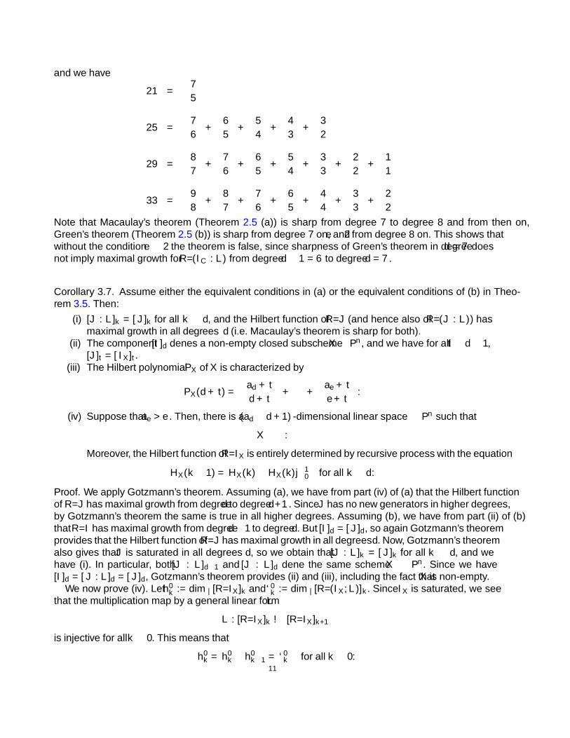
Corollary 3.7. Assume either the equivalent conditions in (a) or the equivalent conditions of (b) in Theo-rem 3.5. Then:
(i) [J : L]k = [J ]k for all k ≥ d, and the Hilbert function of R/J (and hence also of R/(J : L)) hasmaximal growth in all degrees ≥ d (i.e. Macaulay’s theorem is sharp for both).
(ii) The component [I]d defines a non-empty closed subscheme X ⊂ Pn, and we have for all t ≥ d− 1,[J ]t = [IX]t.
(iii) The Hilbert polynomial PX of X is characterized by
PX(d+ t) =
(ad + t
d+ t
)+ · · ·+
(ae + t
e+ t
).
(iv) Suppose that ae > e. Then, there is a (ad − d+ 1)-dimensional linear space Λ ⊂ Pn such that
X ⊂ Λ.
Moreover, the Hilbert function ofR/IX is entirely determined by recursive process with the equation
HX(k − 1) = HX(k)−HX(k)|−10 for all k ≤ d.
Proof. We apply Gotzmann’s theorem. Assuming (a), we have from part (iv) of (a) that the Hilbert functionofR/J has maximal growth from degree d to degree d+1. Since J has no new generators in higher degrees,by Gotzmann’s theorem the same is true in all higher degrees. Assuming (b), we have from part (ii) of (b)that R/I has maximal growth from degree d− 1 to degree d. But [I]d = [J ]d, so again Gotzmann’s theoremprovides that the Hilbert function ofR/J has maximal growth in all degrees≥ d. Now, Gotzmann’s theoremalso gives that J is saturated in all degrees ≥ d, so we obtain that [J : L]k = [J ]k for all k ≥ d, and wehave (i). In particular, both [J : L]d−1 and [J : L]d define the same scheme X ⊂ Pn. Since we have[I]d = [J : L]d = [J ]d, Gotzmann’s theorem provides (ii) and (iii), including the fact that X is non-empty.
We now prove (iv). Let h′k := dimk[R/IX]k and `′k := dimk[R/(IX, L)]k. Since IX is saturated, we seethat the multiplication map by a general linear form L
×L : [R/IX]k → [R/IX]k+1
is injective for all k ≥ 0. This means that
∆h′k = h′k − h′k−1 = `′k for all k ≥ 0.11

Consider the d-th binomial expansion of h′d
h′d =
(add
)+
(ad−1
d− 1
)+ · · ·+
(aee
).
By assumption we have`′d = (h′d) |−1
0 .
For general linear forms L and L′,
(3.8)
(h′d−1)(d−1) |−10 ≥ `′d−1 (by Theorem 2.5 (b))
≥ `′d − dimk[R/(IX, L, L′)]d
= (h′d)(d) |−10 −dimk[R/(IX, L, L
′)]d
≥ (h′d)(d) |−10 −(h′d)(d) |−2
0 .
Now we will show that the first and last of these are equal, making all the intermediate values equal as well.
Claim: if ae > e then (h′d−1)(d−1) |−10= (h′d)(d) |−1
0 −(h′d)(d) |−20 .
The claim follows by the same argument as in the proof of Lemma 3.1 in [1], but we include the detailsfor completeness.
By the assumption that `′d = (h′d)(d) |−10, we have
(3.9)
h′d−1 = h′d − `′d= h′d − [(h′d)(d)] |
−10
=
[(add
)+
(ad−1d− 1
)+ · · ·+
(aee
)]−[(ad − 1
d
)+
(ad−1 − 1
d− 1
)+ · · ·+
(ae − 1
e
)]
=
(ad − 1
d− 1
)+
(ad−1 − 1
d− 2
)+ · · ·+
(ae − 1
e− 1
), if e ≥ 2,(
ad − 1
d− 1
)+
(ad−1 − 1
d− 2
)+ · · ·+
(aδ+1 − 1
δ
)+
(aδδ − 1
), if e = 1,
where δ = max{ i ≥ 2 | ai − i = a2 − 2} and the latter is a routine calculation.Hence we obtain that
(h′d−1)(d−1) |−10=
(ad − 2
d− 1
)+
(ad−1 − 2
d− 2
)+ · · ·+
(ae − 2
e− 1
), if e ≥ 2,(
ad − 2
d− 1
)+
(ad−1 − 2
d− 2
)+ · · ·+
(aδ+1 − 2
δ
)+
(aδ − 1
δ − 1
), if e = 1.
On the other hand, since ae > e we have
(h′d)(d) |−10 −(h′d)(d) |−2
0
=
[(ad − 1
d
)+
(ad−1 − 1
d− 1
)+ · · ·+
(ae − 1
e
)]−[(ad − 2
d
)+
(ad−1 − 2
d− 1
)+ · · ·+
(ae − 2
e
)]
=
(ad − 2
d− 1
)+
(ad−1 − 2
d− 2
)+ · · ·+
(ae − 2
e− 1
), if e ≥ 2,(
ad − 2
d− 1
)+
(ad−1 − 2
d− 2
)+ · · ·+
(aδ+1 − 2
δ
)+
(aδ − 1
δ − 1
), if e = 1
and the claim is proved.So we have equalities in (3.8), and hence
`′d−1 = (h′d−1)(d−1) |−10 .
12
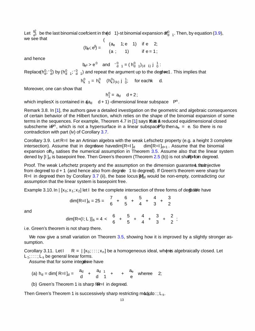
Let(b′ee′
)be the last binomial coefficient in the (d−1)-st binomial expansion of h′d−1. Then, by equation (3.9),
we see that
(be′ , e′) =
{(ae − 1, e− 1) if e ≥ 2,
(aδ, δ − 1) if e = 1,
and hencebe′ > e′ and `′d−1 = (h′d−1)(d−1) |−1
0 .
Replace (h′d, `′d) by (h′d−1, `
′d−1) and repeat the argument up to the degree d = 1. This implies that
h′k−1 = h′k − (h′k)(k) |−10, for each k ≤ d.
Moreover, one can show thath′1 = ad − d+ 2,
which implies X is contained in a (ad − d+ 1)-dimensional linear subspace Λ ⊂ Pn. �
Remark 3.8. In [1], the authors gave a detailed investigation on the geometric and algebraic consequencesof certain behavior of the Hilbert function, which relies on the shape of the binomial expansion of someterms in the sequences. For example, Theorem 4.7 in [1] says that if X is a reduced equidimensional closedsubscheme in Pn, which is not a hypersurface in a linear subspace in Pn, then ae = e. So there is nocontradiction with part (iv) of Corollary 3.7.
Corollary 3.9. Let R/I be an Artinian algebra with the weak Lefschetz property (e.g. a height 3 completeintersection). Assume that in degree d we have dim[R/I]d ≤ dim[R/I]d+1. Assume that the binomialexpansion of hd satisfies the numerical assumption in Theorem 3.5. Assume also that the linear systemdefined by [I]d is basepoint free. Then Green’s theorem (Theorem 2.5 (b)) is not sharp for R/I in degree d.
Proof. The weak Lefschetz property and the assumption on the dimension guarantee that ×L is injectivefrom degree d to d + 1 (and hence also from degree d − 1 to degree d). If Green’s theorem were sharp forR/I in degree d then by Corollary 3.7 (ii), the base locus of [I]d would be non-empty, contradicting ourassumption that the linear system is basepoint free. �
Example 3.10. In k[x0, x1, x2] let I be the complete intersection of three forms of degree 6. We have
dim[R/I]6 = 25 =
(7
6
)+
(6
5
)+
(5
4
)+
(4
3
)+
(3
2
)and
dim[R/(I, L)]6 = 4 <
(6
6
)+
(5
5
)+
(4
4
)+
(3
3
)+
(2
2
),
i.e. Green’s theorem is not sharp there.
We now give a small variation on Theorem 3.5, showing how it is improved by a slightly stronger as-sumption.
Corollary 3.11. Let I ⊂ R = k[x0, . . . , xn] be a homogeneous ideal, where k is algebraically closed. LetL1, . . . , Ls be general linear forms.
Assume that for some integer d we have
(a) hd = dim[R/I]d =
(add
)+
(ad−1
d− 1
)+ · · ·+
(aee
)where e ≥ 2;
(b) Green’s Theorem 1 is sharp for R/I in degree d.
Then Green’s Theorem 1 is successively sharp restricting modulo L1, . . . , Ls.13

Proof. We use the calculations from the previous result. Consider the diagram
(3.10)
0 0 0↓ ↓ ↓
[R/((I : L1) : L2)]d−2 [R/(I : L2)]d−1 [R/((I, L1) : L2)]d−1
↓×L2 ↓×L2 ↓×L2
0 → [R/(I : L1)]d−1×L1−→ [R/I]d → [R/(I, L1)]d → 0
↓ ↓ ↓[R/((I : L1), L2)]d−1 [R/(I, L2)]d [R/(I, L1, L2)]d
↓ ↓ ↓0 0 0
Looking at the first column of (3.10), Green’s Theorem 1 then gives
dim[R/((I : L1), L2)]d−1 ≤(ad − 2
d− 1
)+ · · ·+
(ae − 2
e− 1
).
It is important to note that this holds even if ae = e. What is important is the condition e ≥ 2.Because we assumed that Green’s Theorem 1 is sharp for R/I in degree d, we can apply Green’s Theo-
rem 1 again to R/(I, L1) and we have
dim[R/(I, L1, L2)]d ≤ (hd)|−20 =
(ad − 2
d
)+ · · ·+
(ae − 2
e
).
Since((I, L2) : L1) ⊇ ((I : L1), L2),
we obtaindim[R/((I, L2) : L1)]d−1 ≤ dim[R/((I : L1), L2)]d−1
≤(ad − 2
d− 1
)+ · · ·+
(ae − 2
e− 1
).
The sequence0→ [R/((I, L2) : L1)]d−1 → [R/(I, L2)]d → [R/(I, L1, L2)]d → 0
then gives(ad − 1
d
)+ · · ·+
(ae − 1
e
)= dim[R/(I, L2)]d
= dim[R/((I, L2) : L1)]d−1 + dim[R/(I, L1, L2)]d
≤[(ad − 2
d− 1
)+ · · ·+
(ae − 2
e− 1
)]+
[(ad − 2
d
)+ · · ·+
(ae − 2
e
)]=
(ad − 1
d
)+ · · ·+
(ae − 1
e
).
Again notice that this holds even if ae = e. We conclude
dim[R/((I, L2) : L1)]d−1 =
(ad − 2
d− 1
)+ · · ·+
(ae − 2
e− 1
)and
(3.11)dim[R/(I, L1, L2)]d =
(ad − 2
d
)+ · · ·+
(ae − 2
e
)= (hd)|−2
0.14

Now replace I by (I, L1) and repeat the argument, adding one linear form at a time, continuing through Ls.�
The following result will be useful in the next section. It makes only an injectivity assumption (equivalentto a certain numerical assumption, as noted in Lemma 3.4). Note also the similarity to Lemma 2.9, and to[23, Proposition 2.1 (b)], although this proof is completely different. In the next section this will be of useto us.
Lemma 3.12. For a general linear form L in R = k[x0, . . . , xn] assume that
×L : [R/I]d → [R/I]d+1
is injective (i.e. hd − hd+1 + `d+1 = 0), and that
×L : [R/I]d−1 → [R/I]d
has an s-dimensional kernel (i.e. hd−1−hd+`d = s). ThenR/I has an s-dimensional socle in degree d−1.
Proof. Let L0, . . . , Ln be n+ 1 general linear forms. Note that they form a basis for [R]1. Choose any two,Li and Lj and consider the following commutative diagram:
0↓[I:Lj
I
]d−1
0
↓ ↓0 →
[I:LiI
]d−1
→ [R/I]d−1×Li−→ [R/I]d → [R/(I, Li)]d → 0
↓ ×Lj ↓ ×Lj
0 → [R/I]d×Li−→ [R/I]d+1 → [R/(I, Li)]d+1 → 0
An easy diagram chase shows that the kernel of multiplication by Li is the same as the kernel of multipli-cation by Lj . Since L0, . . . , Ln form a basis for [R]1, this kernel is contained in the kernel of multiplicationby any linear form, and we are done. �
4. CLASSIFICATION OF GORENSTEIN SEQUENCES OF THE FORM (1, r, r − 2, r, 1)
As indicated in the introduction, a great deal of research has gone into the study of possible GorensteinHilbert functions (i.e. Gorenstein sequences). As a subproblem, it has been of great interest to understandwhen they can be unimodal. In the recent paper [28] this was solved for socle degrees 4 and 5. However, thisfell short of a classification of the possible Hilbert functions even in socle degree 4 – what is missing is tocompletely understand the extent of non-unimodality that occurs. What is now known thanks to that paperis a classification of the possible Gorenstein Hilbert functions of the form (1, r, r − 1, r, 1). However, eventhe case (1, r, r−2, r, 1) is open. In this section we complete this case, as well as an analogous one for socledegree 5 (see Corollary 4.3).
In [28] it was observed in Remark 3.5 that (1, 20, 18, 20, 1) is a Gorenstein Hilbert function, arisingeasily using trivial extensions. It will then follow from Theorem 2.12 that this is the smallest possible of theform (1, r, r − 2, r, 1) (and by Theorem 2.12 all values r ≥ 20 also exist) once we show that the h-vectorH = (1, 19, 17, 19, 1) is not a Gorenstein sequence. We do this using results from the previous section. Wewill use without comment Notation 2.3. The characteristic assumption is only to be able to use Theorem 3.2.
Theorem 4.1. Assume that char k = 0. Then the h-vector H = (1, 19, 17, 19, 1) is not Gorenstein.
Proof. Assume that there exists an Artinian Gorenstein algebraR/I with Hilbert function H. Let J = 〈I≤3〉be the ideal generated by the components of I in degrees ≤ 3. Then, by Macaulay’s theorem,
H(R/J, 4) ≤ 31.
15

(i) If H(R/J, 4) = 31 then the Hilbert function of R/J has maximal growth in degree 3. So byLemma 2.9, R/J has a 7-dimensional socle elements in degree 2, and hence so does R/I . Thiscontradicts the Gorenstein assumption.
(ii) If H(R/J, 4) = 30, then the Betti table of R/J lex (after truncating in degree 4) is of the form
0 1 · · · · · · 18 190 1 0 · · · · · · 0 01 0 173 · · · · · · 247 132 0 19 · · · · · · 131 73 0 1 · · · · · · 0 04 0 43 · · · · · · 551 30
Using the Cancellation Principle (see [29]), we get that R/J has a socle element in degree 2, andhence so does R/I , which is a contradiction.
(iii) If H(R/J, 4) = 29, then the Betti table of R/J lex (after truncating in degree 4) is of the form
0 1 · · · · · · 18 190 1 0 · · · · · · 0 01 0 173 · · · · · · 247 132 0 19 · · · · · · 131 73 0 2 · · · · · · 1 04 0 41 · · · · · · 532 29
Again using the Canclellation Principle, we get that R/J has a socle element in degree 2, and henceso does R/I , which is a contradiction.
As a result, we have:
Without loss of generality we can assume that H(R/J, 4) ≤ 28.
Since we must have`3 ≤ (`2)(2)|+1
+1 and `3 ≤ (h3)(3)|−10
as well has having the middle line symmetric (Gorenstein), there are three possibilities for the decompositionof H. They are
1 19 17 19 11 10 10 1
1 18 7 9
1 19 17 19 11 11 11 1
1 18 6 8
1 19 17 19 11 12 12 1
1 18 5 7
Case 1. We consider the first decomposition of H, namely
(4.1)1 19 17 19 1
1 10 10 11 18 7 9
Since
h(3) = 19(3) =
(2 + 3
3
)+
(2 + 2
2
)+
(2 + 1
1
)and `3 = 9 = 19(3)
∣∣−1
0,
by Theorem 3.2, there is a 3-dimensional linear space Λ such that J3 defines a hypersurface F of degree 3in Λ ⊂ P18 (and is saturated in degree 3). Since J is generated in degrees ≤ 3, the Hilbert function of R/Jis
H(R/J, t) =
(2 + t
t
)+
(2 + (t− 1)
(t− 1)
)+
(2 + (t− 2)
(t− 2)
), for all t ≥ 3,
16
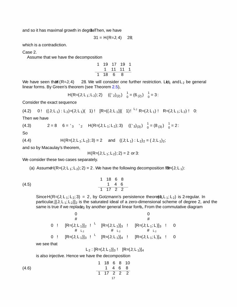
and so it has maximal growth in degree 3. Then, we have
31 = H(R/J, 4) ≤ 28,
which is a contradiction.
Case 2.Assume that we have the decomposition
1 19 17 19 11 11 11 1
1 18 6 8
We have seen that H(R/J, 4) ≤ 28. We will consider one further restriction. Let L1 and L2 be generallinear forms. By Green’s theorem (see Theorem 2.5),
H(R/(J, L1, L2), 2) ≤ ((`2)(2))∣∣−1
0= (6(2))
∣∣−1
0= 3.
Consider the exact sequence
(4.2) 0→ ((J, L1) : L2)/(J, L1)(−1)→ [R/((J, L1)](−1)×L2−→ R/(J, L1)→ R/(J, L1, L2)→ 0.
Then we have
(4.3) 2 = 8− 6 = `3 − `2 ≤ H(R/(J, L1, L2), 3) ≤ ((`3)(3))∣∣−1
0= (8(3))
∣∣−1
0= 2.
So
(4.4) H(R/(J, L1, L2), 3) = 2 and ((J, L1) : L2)2 = (J, L1)2,
and so by Macaulay’s theorem,H(R/(J, L1, L2), 2) = 2 or 3.
We consider these two cases separately.
(a) Assume H(R/(J, L1, L2), 2) = 2. We have the following decomposition for R/(J, L1):
(4.5)1 18 6 8
1 4 61 17 2 2
Since H(R/(J, L1, L2, 3) = 2, by Gotzmann’s persistence theorem, (J, L1, L2) is 2-regular. Inparticular, [(J, L1, L2)]2 is the saturated ideal of a zero-dimensional scheme of degree 2, and thesame is true if we replace L2 by another general linear form, L. From the commutative diagram
0 0↓ ↓
0 → [R/(J, L1)]2×L−→ [R/(J, L1)]3 → [R/(J, L1, L)]3 → 0
↓ ×L2 ↓ ×L2 ↓ ×L2
0 → [R/(J, L1)]3×L−→ [R/(J, L1)]4 → [R/(J, L1, L)]4 → 0
we see that×L2 : [R/(J, L1)]3 → [R/(J, L1)]4
is also injective. Hence we have the decomposition
(4.6)1 18 6 8 10
1 4 6 81 17 2 2 2
17
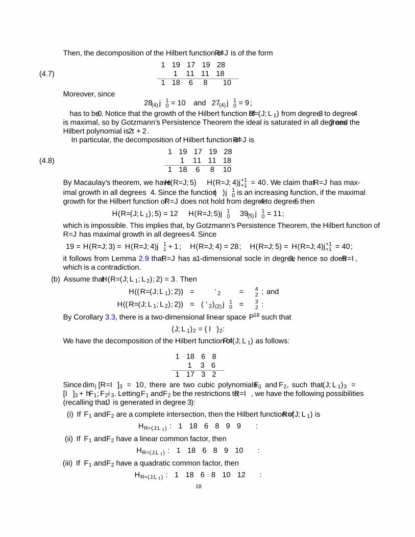
Then, the decomposition of the Hilbert function of R/J is of the form
(4.7)1 19 17 19 28− α
1 11 11 18− α1 18 6 8 10
Moreover, since28(4)|−1
0 = 10 and 27(4)|−10 = 9,
α has to be 0. Notice that the growth of the Hilbert function of R/(J, L1) from degree 3 to degree 4is maximal, so by Gotzmann’s Persistence Theorem the ideal is saturated in all degrees ≥ 3 and theHilbert polynomial is 2t+ 2.
In particular, the decomposition of Hilbert function of R/J is
(4.8)1 19 17 19 28
1 11 11 181 18 6 8 10
By Macaulay’s theorem, we have H(R/J, 5) ≤ H(R/J, 4)|+1+1 = 40. We claim that R/J has max-
imal growth in all degrees ≥ 4. Since the function (−)|−10 is an increasing function, if the maximal
growth for the Hilbert function of R/J does not hold from degree 4 to degree 5 then
H(R/(J, L1), 5) = 12 ≤ H(R/J, 5)|−10 ≤ 39(5)|−1
0 = 11,
which is impossible. This implies that, by Gotzmann’s Persistence Theorem, the Hilbert function ofR/J has maximal growth in all degrees ≥ 4. Since
19 = H(R/J, 3) = H(R/J, 4)|−1−1 + 1, H(R/J, 4) = 28, H(R/J, 5) = H(R/J, 4)|+1
+1 = 40,
it follows from Lemma 2.9 that R/J has a 1-dimensional socle in degree 3, hence so does R/I ,which is a contradiction.
(b) Assume that H(R/(J, L1, L2), 2) = 3. Then
H((R/(J, L1), 2)) = `2 =(
42
), and
H((R/(J, L1, L2), 2)) = (`2)(2)|−10 =
(32
).
By Corollary 3.3, there is a two-dimensional linear space Λ ⊂ P18 such that
(J, L1)2 = (IΛ)2.
We have the decomposition of the Hilbert function of R/(J, L1) as follows:
1 18 6 81 3 6
1 17 3 2
Since dimk[R/IΛ]3 = 10, there are two cubic polynomials, F1 and F2, such that (J, L1)3 =[IΛ]3 + 〈F1, F2〉3. Letting F̄1 and F̄2 be the restrictions to R/IΛ, we have the following possibilities(recalling that J is generated in degree ≤ 3):
(i) If F̄1 and F̄2 are a complete intersection, then the Hilbert function of R/(J, L1) is
HR/(J,L1) : 1 18 6 8 9 9 · · · .
(ii) If F̄1 and F̄2 have a linear common factor, then
HR/(J,L1) : 1 18 6 8 9 10 · · · .
(iii) If F̄1 and F̄2 have a quadratic common factor, then
HR/(J,L1) : 1 18 6 8 10 12 · · · .18

In all of these cases, we claim that the ideal (J, L1) is saturated in degree≥ 3. Indeed, (i) is a heighttwo complete intersection and (ii) and (iii) are ideals of the form F ·K where F is a homogeneouspolynomial and K is a height two complete intersection. Then we have that for any d ≥ 3,
[(J, L1)]satd = (J, L1)d ⊆ ((J : L2), L1)d ⊆ (J sat, L1)d ⊆ [(J, L1)]sat
d .
Hence,H(R/((J : L2), L1), 3) = H(R/(J, L1), 3) = 8.
Remembering that both L1 and L2 are general linear forms and that
H(R/(J : L1), 3) ≤ h3 = 19,
this means that H(R/(J : L1), 3) is either 19 or 18.Now recall that we assume that H(R/J, 4) ≤ 28 and
(27)(4)|−10 = 9 and (28)(4)|−1
0 = 10.
It follows that there are three possible decompositions of the Hilbert function H, namely
1 19 17 19 281 11 11 19
1 18 6 8 9or
1 19 17 19 281 11 11 18
1 18 6 8 10or
1 19 17 19 271 11 11 18
1 18 6 8 9
The first is eliminated using Lemma 3.12. The second was already eliminated in part (a) of the proof.We thus focus on the third possibility, and we include a consideration of what happens in degree 4.Note that it suffices to consider either case (i) or case (ii) above, since H(R/(J, L1), 4) = 10 in case(iii).
First consider case (i). We know that J sat defines the union of a set of m ≥ 0 points and a curve,C in P3, of degree 9 whose general hyperplane section is the complete intersection of two cubics inthe plane. By [32] or [22], C must be the complete intersection of two cubic surfaces in P3. Thusthe Hilbert polynomial of R/J sat is 9t − 9 + m, so by looking in degree 4 we see m = 0 and[J ]4 = [J sat]4. Then for a general linear form ×L : [R/J ]4 → [R/J ]5 is injective, but the same isnot true from degree 3 to degree 4, so by Lemma 3.12 R/J has socle in degree 3. Then the same istrue of R/I , and we have a contradiction.
Now consider case (ii). Note that the Hilbert polynomial of R/(J, L1) is t+ 5 and
(J, L1)≥2 = (LG1, LG2)≥2 (mod IΛ).
So (J, L1) is the saturated ideal of the union of a line L = V (L) and a zero-dimensional completeintersection subscheme Y = V (G1, G2) of degree 4 in a plane Λ (in this case, Y is not necessarilyreduced or irreducible, and the complete intersection Y contains at most a subscheme of degree 2embedded in the line).
Now consider J sat. In degree≥ 3 it defines the scheme-theoretic union (in a 3-dimensional linearspace Π) of a plane, a one-dimensional subscheme C of degree 4, and possibly a 0-dimensionalscheme of finite length. Since modulo IΛ the ideal (J, L1) has the form (LG1, LG2) where G1 andG2 are a complete intersection, so C must be defined by two quadrics Q1, Q2, i.e. it must be acomplete intersection. So J sat defines a scheme X that contains a subscheme (viewed in P3) definedby an ideal of the form (LQ1, LQ2). But since
27 = H(R/(LQ1, LQ2), 4) ≤ H(R/IX, 4) = H(R/J sat, 4) ≤ H(R/J, 4) = 27,
the ideal J sat is saturated in degree 4, and the same argument that we used for (i) works here.
Case 3. Now consider the last decomposition of H, namely
(4.9)1 19 17 19 1
1 12 12 11 18 5 7
19

Note that, by the Gotzmann persistence theorem, the ideal [(J, L)] is 2-regular and [(J, L)/(L)] defines aconic in a two dimensional linear space in L ∼= P17. In particular, H(R/(J, L), 4) = 9. This implies thatJ sat defines the union of a quadric hypersurface F = V (F ) in a 3-dimensional linear space Λ ⊂ P18 anda finite scheme Y of degree m in P18 (in this case, a quadric form F defining F need not to be reduced orirreducible.). Hence we have the following decomposition for R/J .
(4.10)1 19 17 19 28− α
1 12 12 19− α1 18 5 7 9
Note that
28 ≥ H(R/J, 4) ≥ H(R/J sat, 4) =
(6
4
)+
(5
3
)+m = 25 +m,
which implies that 0 ≤ m ≤ 3 and 0 ≤ α ≤ 3.We first observe that if H(R/J, 4) = 28 then α = 0. Hence in the notation of Lemma 3.12, we have
h3 − h4 + `4 = 19− 28 + 9 = 0 and h2 − h3 + `3 = 17− 19 + 7 = 5.
It follows from Lemma 3.12 thatR/J has a 5-dimensional socle in degree 2. HenceR/I does as well, whichis a contradiction. Thus from now on we assume that H(R/J, 4) ≤ 27, and consequently m ≤ 2.
(i) Assume m = 2. Then H(R/J, 4) = 27. We claim that the Hilbert function of R/J has maximalgrowth in degree 4. Indeed, by Macaulay’s theorem, we see that
H(R/J, 5) ≤ H(R/J, 4)|+1+1 = 38.
If this inequality is not sharp, we have H(R/J, 5) ≤ 37 =(
75
)+(
64
)+(
33
). This implies that, by
Macaulay’s theorem,
H(R/J, d) ≤(d+ 2
d
)+
(d+ 1
d− 1
)+
(d− 2
d− 2
), for each d ≥ 5.
Since J sat defines 2-dimensional subscheme of degree 2, the Hilbert polynomial of R/J sat is either
PR/Jsat(d) =
(d+ 2
d
)+
(d+ 1
d− 1
)or PR/Jsat(d) =
(d+ 2
d
)+
(d+ 1
d− 1
)+
(d− 2
d− 2
),
which implies that m = 0 or m = 1 respectively. This is a contradiction to the assumption thatm = 2. Hence the Hilbert function of R/J has maximal growth in degree 4. By Lemma 3.12, R/J(and hence R/I) has a one dimensional socle in degree 3. This is a contradiction.
(ii) Assume m = 1. In this case, H(R/J, 4) is either 26 or 27. In the first case J is saturated in degree4, so H(R/J, 5) = 37. We have the following possibilities:
d 0 1 2 3 4 5 k ≥ 6 · · ·Case 1 : H(R/J, d) 1 19 17 19 26 37
(k+2k
)+(k+1k−1
)+(k−2k−2
)· · ·
Case 2 : H(R/J, d) 1 19 17 19 27 37(k+2k
)+(k+1k−1
)+(k−2k−2
)· · ·
Case 3 : H(R/J, d) 1 19 17 19 27 ≥ 38(k+2k
)+(k+1k−1
)+(k−2k−2
)· · ·
For the first case, the Hilbert function of R/J has maximal growth in degree 4. By Lemma 3.12,R/I has two dimensional socle in degree 3. This is a contradiction.
In the second case, J sat defines the union of a quadric surface in 3-dimensional space and onepoint. By the Gorenstein hypothesis,R/J has no socle element in degree≤ 3. LetA = R/(J+m5)and B = R/(J sat + m5), where m is the irrelevant maximal ideal of R. We denote by hA(−) andhB(−) the Hilbert function of A and B respectively. Then
(1, hA(3)− hB(3), hA(2)− hB(2), . . . ) = (1, 2, 7, . . . )20
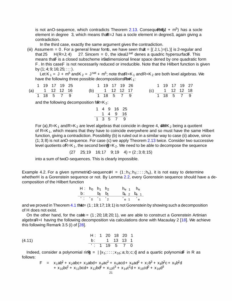
is not an O-sequence, which contradicts Theorem 2.13. Consequently, R/(J + m5) has a socleelement in degree ≤ 3, which means that R/J has a socle element in degree ≤ 3, again giving acontradiction.
In the third case, exactly the same argument gives the contradiction.(iii) Assume m = 0. For a general linear form L, we have seen that J̄ = [(J, L)/(L)] is 2-regular and
that 25 ≤ H(R/J, 4) ≤ 27. Since m = 0, the ideal J sat defines a quadric hypersurface F. Thismeans that F is a closed subscheme in a 3-dimensional linear space defined by one quadratic formF . In this case, F is not necessarily reduced or irreducible. Note that the Hilbert function is givenby (1, 4, 9, 16, 25, . . . ).
Let K1 = J + m5 and K2 = J sat + m5; note that R/K1 and R/K2 are both level algebras. Wehave the following three possible decompositions for R/K1:
(a)1 19 17 19 25
1 12 12 161 18 5 7 9
(b)1 19 17 19 26
1 12 12 171 18 5 7 9
(c)1 19 17 19 27
1 12 12 181 18 5 7 9
and the following decomposition for R/K2:
1 4 9 16 251 4 9 16
1 3 5 7 9
For (a), R/K1 and R/K2 are level algebras that coincide in degree 4, with R/K2 being a quotientof R/K1, which means that they have to coincide everywhere and so must have the same Hilbertfunction, giving a contradiction. Possibility (b) is ruled out in a similar way to case (ii) above, since(1, 3, 8) is not an O-sequence. For case (c) we apply Theorem 2.13 twice. Consider two successivelevel quotients of R/K1, the second being R/K2. We need to be able to decompose the sequence
(27− 25, 19− 16, 17− 9, 19− 4) = (2, 3, 8, 15)
into a sum of two O-sequences. This is clearly impossible.�
Example 4.2. For a given symmetric O-sequence H = (1, h1, h2, . . . , he), it is not easy to determinewhether H is a Gorenstein sequence or not. By Lemma 2.2, every Gorenstein sequence should have a de-composition of the Hilbert function
H : h0 h1 h2 · · · he−1 heb : b0 b1 · · · be−2 be−1
` : `0 `1 `2 · · · `e−1 `e
and we proved in Theorem 4.1 that H = (1, 19, 17, 19, 1) is not Gorenstein by showing such a decompositionof H does not exist.
On the other hand, for the case H = (1, 20, 18, 20, 1), we are able to construct a Gorenstein Artinianalgebra R/I having the following decomposition via calculations done with Macaulay 2 [18]. We achievethis following Remark 3.5 (i) of [28].
(4.11)H : 1 20 18 20 1b : 1 13 13 1` : 1 19 5 7 0
Indeed, consider a polynomial ring R = k[x1, . . . , x16, a, b, c, d] and a quartic polynomial F in R asfollows:
F = x1ab2 + x2abc+ x3abd+ x4ac
2 + x5acd+ x6ad2 + x7b
3 + x8b2c+ x9b
2d+x10bc
2 + x11bcd+ x12bd2 + x13c
3 + x14c2d+ x15cd
2 + x16d3
21
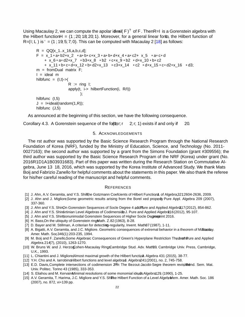
Using Macaulay 2, we can compute the apolar ideal I = (F )⊥ of F . Then R/I is a Gorenstein algebra withthe Hilbert function H = (1, 20, 18, 20, 1). Moreover, for a general linear form L, the Hilbert function ofR/(I, L) is ` = (1, 19, 5, 7, 0). This can be computed with Macaulay 2 [18] as follows:
R = QQ[x_1..x_16,a,b,c,d];F = x_1*a*bˆ2+x_2*a*b*c+x_3*a*b*d+x_4*a*cˆ2+ x_5*a*c*d
+ x_6*a*dˆ2+x_7*bˆ3+x_8*bˆ2*c+x_9*bˆ2*d+x_10*b*cˆ2+ x_11*b*c*d+x_12*b*dˆ2+x_13*cˆ3+x_14*cˆ2*d+x_15*c*dˆ2+x_16*dˆ3;
m = fromDual matrix F;I = ideal mhilbfunc = (I,t)->(
R := ring I;apply(t, i-> hilbertFunction(i, R/I))
);hilbfunc (I,5)J = I+ideal(random(1,R));hilbfunc (J,5)
As announced at the beginning of this section, we have the following consequence.
Corollary 4.3. A Gorenstein sequence of the form (1, r, r − 2, r, 1) exists if and only if r ≥ 20.
5. ACKNOWLEDGEMENTS
The first author was supported by the Basic Science Research Program through the National ResearchFoundation of Korea (NRF), funded by the Ministry of Education, Science, and Technology (No. 2011-0027163); the second author was supported by a grant from the Simons Foundation (grant #309556); thethird author was supported by the Basic Science Research Program of the NRF (Korea) under grant (No.2016R1D1A1B03931683). Part of this paper was written during the Research Station on Commutative Al-gebra, June 13 – 18, 2016, which was supported by the Korea Institute of Advanced Study. We thank MatsBoij and Fabrizio Zanello for helpful comments about the statements in this paper. We also thank the refereefor his/her careful reading of the manuscript and helpful comments.
REFERENCES
[1] J. Ahn, A.V. Geramita, and Y.S. Shin, The Gotzmann Coefficients of Hilbert Functions, J. of Algebra, 321:2604-2636, 2009.[2] J. Ahn and J. Migliore, Some geometric results arising from the Borel fixed property, J. Pure Appl. Algebra 209 (2007),
337-360.[3] J. Ahn and Y.S. Shin, On Gorenstein Sequences of Socle Degree 4 and 5, J. Pure and Applied Algebra, 217 (2012), 854-862.[4] J. Ahn and Y.S. Shin, Artinian Level Algebras of Codimension 3, J. Pure and Applied Algebra, 216 (2012), 95-107.[5] J. Ahn and Y.S. Shin, Nonunimodal Gorenstein Sequences of Higher Socle Degrees, preprint 2016.[6] H. Bass, On the ubiquity of Gorenstein rings, Math. Z. 82 (1963), 8-28.[7] D. Bayer and M. Stillman, A criterian for detecting m-regularity, Invent. Math. 87 (1987), 1-11.[8] A. Bigatti, A.V. Geramita, and J.C. Migliore. Geometric consequences of extremal behavior in a theorem of Macaulay. Trans.
Amer. Math. Soc., 346(1):203-235, 1994.[9] M. Boij and F. Zanello, Some Algebraic Consequences of Green’s Hyperplane Restriction Theorems, J. of Pure and Applied
Algebra. 214(7), (2010), 1263-1270.[10] W. Bruns W. and J. Herzog, Cohen-Macaulay Rings, Cambridge Stud. Adv. Math. 39, Cambridge Univ. Press, Cambridge,
U.K., 1993.[11] L. Chiantini and J. Migliore, Almost maximal growth of the Hilbert function, J. Algebra 431 (2015), 38-77.[12] Y.H. Cho and A. Iarrobino, Hilbert functions and level algebras, J. Algebra 241 (2001), no. 2, 745-758.[13] E.D. Davis, Complete intersections of codimension 2 in Pr: The Bezout-Jacobi-Segre theorem revisited, Rend. Sem. Mat.
Univ. Politec. Torino 43 (1985), 333-353.[14] S. Eliahou and M. Kervaire, Minimal resolutions of some monomial ideals, J. Algebra 129, (1990), 1-25.[15] A.V. Geramita, T. Harima, J.C. Migliore and Y.S. Shin. The Hilbert Function of a Level Algebra, Mem. Amer. Math. Soc. 186
(2007), no. 872, vi+139 pp.22

[16] G. Gotzmann. Eine Bedingung für die Flachheit und das Hilbertpolynom eines graduierten Ringes. Math. Z., 158(1):61-70,1978.
[17] M. Green. Restrictions of linear series to hyperplanes, and some results of Macaulay and Gotzmann. In Algebraic curves andprojective geometry (Trento, 1988), volume 1389 of Lecture Notes in Math., pages 76-86. Springer, Berlin, 1989.
[18] Daniel R. Grayson, Michael E. Stillman, Macaulay 2: a software system for algebraic geometry and commutative algebra,available over the web at http://www.math.uiuc.edu/Macaulay2.
[19] T. Harima, Characterization of Hilbert functions of Gorenstein Artin algebras with the weak Stanley property. Proc. Amer.Math. Soc. 123 (1995) 3631-3638.
[20] M. Kreuzer and L. Robbiano. Computational commutative algebra. 2. Springer-Verlag, Berlin, 2005.[21] F.S. Macaulay. Some properties of enumeration in the theory of modular systems, Proc. Lond. Math. Soc., 26(1):531-555,
1927.[22] J. Migliore, Hypersurface sections of curves, in the Proceedings of the International Conference on Zero-Dimensional
Schemes, Ravello 1992, De Gruyter (1994), 269-282.[23] J. Migliore, R. Miró-Roig and U. Nagel, Monomial ideals, almost complete intersections and the Weak Lefschetz Property,
Trans. Amer. Math. Soc. 363 (2010), 229-257.[24] J.C. Migliore, U. Nagel, and F. Zanello, A Characterization of Gorenstein Hilbert Functions in Codimension 4 with Small
Initial Degree, Math. Res. Lett., 15 (2008), 331-349.[25] J. Migliore and U. Nagel, Reduced arithmetically Gorenstein schemes and simplicial polytopes with maximal Betti numbers,
Adv. Math. 180 (2003), 1–63.[26] J. Migliore and U. Nagel, A tour of the weak and strong Lefschetz properties, J. Comm. Alg. 5 (2013), 329–358.[27] J.C. Migliore, U. Nagel, and F. Zanello, , On the degree two entry of a Gorenstein h-vector and a conjecture of Stanley, Proc.
Amer. Math. Soc. 136 (2008), 2755-2762.[28] J.C. Migliore and F. Zanello, Stanley Nonunimodal Gorenstein h-vector is Optimal, to appear in Proc. Amer. Math. Soc.
(arXiv:1512.01433.)[29] I. Peeva, Consecutive cancellations in Betti numbers, Proc. Amer. Math. Soc. 132 (2004), no. 12, 3503-3507.[30] R.P. Stanley. Hilbert functions of graded algebras, Advances in Math., 28(1):57-83, (1978).[31] R.P. Stanley, “Combinatorics and commutative algebra,” First edition. Progress in Mathematics, 41. Birkhäuser Boston, Inc.,
Boston, MA, 1983.[32] R. Strano, A characterization of complete intersection curves in P3, Proc. Amer. Math. Soc. 104 (1988), no. 3, 711-715.[33] F. Zanello: When is there a unique socle-vector associated to a given h-vector?, Comm. Algebra 34 (2006), no. 5, 1847-1860.
DEPARTMENT OF MATHEMATICS EDUCATION, KONGJU NATIONAL UNIVERSITY, 182, SHINKWAN-DONG, KONGJU, CHUNG-NAM 314-701, REPUBLIC OF KOREA
E-mail address: [email protected]
DEPARTMENT OF MATHEMATICS, UNIVERSITY OF NOTRE DAME, NOTRE DAME, IN 46556, USAE-mail address: [email protected]
DEPARTMENT OF MATHEMATICS, SUNGSHIN WOMEN’S UNIVERSITY, SEOUL, REPUBLIC OF KOREA, 136-742E-mail address: [email protected]
23