Contents lists available at ScienceDirect

Journal of Sound and Vibration

Journal of Sound and Vibration 333 (2014) 1781–1795

0022-46http://d

n CorrE-m

journal homepage: www.elsevier.com/locate/jsvi

Green's functions of the forced vibration of Timoshenkobeams with damping effect

X.Y. Li n, X. Zhao, Y.H. LiSchool of Mechanics and Engineering, Southwest Jiaotong University, Chengdu 610031, PR China

a r t i c l e i n f o

Article history:Received 6 August 2013Received in revised form30 October 2013Accepted 2 November 2013

Handling Editor: L.G. Tham

for beams with various boundaries. The present solutions can be readily reduced to those

Available online 3 December 2013

0X/$ - see front matter & 2013 Elsevier Ltd.x.doi.org/10.1016/j.jsv.2013.11.007

esponding author. Tel.: þ86 28 8763 4181;ail addresses: zjuparis6@hotmail.com (X.Y. L

a b s t r a c t

This paper is concerned with the dynamic solutions for forced vibrations of Timoshenkobeams in a systematical manner. Damping effects on the vibrations of the beam are takeninto consideration by introducing two characteristic parameters. Laplace transform methodis applied in the present study and corresponding Green's functions are presented explicitly

for others classical beam models by setting corresponding parameters to zero or infinite.Numerical calculations are performed to validate the present solutions and the effects ofvarious important physical parameters are investigated.

& 2013 Elsevier Ltd. All rights reserved.

1. Introduction

Studies on the dynamic behavior of beams have been the classic and long-standing problem [1–4]. Historically, variousclassic models, such as Euler, Rayleigh and Timoshenko model were sequentially proposed. The forced transverse vibrationof the beam is usually encountered in engineering applications, such as in the design of aircraft structures, bridges,machines and so forth [5–9].

Various approaches have been proposed to solve the forced vibration of the beam. For example, the mode superpositionmethod, which expresses the solutions by an infinite series, prevailed in the literature [10,11]. In practice, however, truncationsare definitely used during the course of computation of the infinite series. Consequently, the mode superposition method isessentially an approximate one.

In contrast to the mode superposition method, closed form Green's functions play an important role in digging thephysical essences of the problem in question [12–14]. A great deal of effort has been made to derive the correspondingGreen's functions. Lueschen et al. [15], for instance, performed the Laplace transform with respect to time variable involvedin the differential equation governing the forced vibrations of a Timoshenko beam (TB), and obtained the correspondingGreen's function in the frequency domain. However, the solutions in the time domain cannot be derived because of thedifficulties in evaluating the corresponding inverse Laplace transforms. Using the method in Ref. [15], Lin and Lee [16]studied the forced vibration of a curve TB with a circular cross section, and obtained the corresponding fundamentalsolution in integral forms.

Variable separation technique is also adopted to obtain Green's functions, for the steady-state dynamics of a beamsubjected to an external stimulus. For the forced vibration of an Euler beam (EB), Abu-Hilal [17], with the help of the Laplacetransformwith respect to the spatial variable in the governing differential equations, presented a set of Green's functions for

All rights reserved.

fax: þ86 28 8760 0797.i), zhaoxiang_swjtu@hotmail.com (X. Zhao), yinghui.li@home.swjtu.edu.cn (Y.H. Li).

X.Y. Li et al. / Journal of Sound and Vibration 333 (2014) 1781–17951782

the EB with various boundary conditions. Taking advantage of the variable separation method, Foda and Abdul-Jabbar [18]investigated the dynamic behavior of a simply supported EB under the action of a mass moving with a constant speed.

Physically, Green's function Gðx; x0Þ of a system represents the response at the receiver at the position x as a result ofa source at the location x0. It is mathematically viewed as an influence function involved in integral equations, whichhave been systematically studied a century before, by Voltera, Fredholm, Hilbert and some other scientists [19,20]. For amathematical point of view, a partial differential equation denotes a relationship between the values of given and unknownfunctions in an infinitesimal interval, whereas an integral equation involves a finite interval [21]. It is noted that integralequations for a linear system can be established by corresponding Green's function by virtue of superposition principle.For example, integral equations and integro-differential equations are constructed for contact and crack problems, in thecontext of theory of elasticity for multi-field coupling media, as evidenced by Chen et al. [22] for piezo-electric material andChen et al. [23] for magneto-electro-elastic composites.

As pointed out by Duffy [24], Green's functions are very beneficial to constructing the solutions for more involvedproblems, with the help of superposition principle. Starting from the steady-state Green's function, Sun [25], by virtue ofthe Fourier transform, developed a closed-form solution for an EB subjected to a line harmonic load, on a visco-elasticfoundation. Utilizing the properties of Green's functions, Kidawa-Kukla [26] employed a time partitioning method toexamine the transverse vibration induced by a mobile heat source. Extended works on the applications of the dynamicGreen's functions of beams can be referred to in Refs. [27–32].

From an overall point of view, the damping effects are not considered in most of the previous works. In fact, the dampingeffects are important in engineering applications. To the best of authors' knowledge, there is no report published yet inliterature concerning Green's function of TB with damping effect.

In the present paper, we aim to develop the steady-state Green's functions for forced vibrations of TB with dampingeffects. Starting from the basic equations, we sequentially employ the variable separation technique and the Laplacetransforms, to derive Green's functions, where all the constants involved are determined by the boundary conditions.The present fundamental solutions can be readily reduced to those for the classic Timoshenko beamwithout damping effect,Rayleigh beam (RB) and Euler beam (EB), simply by setting some physical quantities to zero or infinite. Numericalcalculations are performed to discuss the validity of the present solutions, and show the effects of various geometrical andphysical quantities of special interests. The present solutions, which are given in a closed and explicit form, can serve asbenchmarks to computational methods. Furthermore, the present solutions can be employed to construct the analyses formore involved problems, as shown in the recent studies [27,28,31].

2. Governing equations for TB with damping effect

First, we consider the dynamic equation of the TB [33]

EIψ″þκGAðw′�ψÞ�c2 _ψ�γ €ψ ¼ 0 (1a)

κGAðw″�ψ ′Þ�c1 _w�μ €w¼ pðx; tÞ (1b)

where ψ and w denotes the rotation angle and the transverse displacement, respectively; EI and κGA represent the bendingand shear stiffness modules; c1 and c2 are two variables characterizing the translational and rotational damping effects,respectively; γ and μ respectively stand for the rotational inertia and the mass per unit length of the beam; p(x, t) denotesthe load applied on the beam and κ is the shear correction factor. In addition, the conventional differential symbols are usedin (1), more precisely; the dot denotes a derivative with respect to timet, and the prime indicates a derivative with respect tothe spatial coordinate x.

For convenience, Eq. (1) can be simplified into a differential equation of the variable w by eliminating the variable ψ .From (1b), it is seen that

ψ ′¼w″� c1κGA

_w� μ

κGA€w� 1

κGApðx; tÞ: (2)

Differentiating (1a) with respect to x and using (2), we can arrive at

EIw′′′′� EIc1κGA

þc2

� �_w″� EIμ

κGAþγ

� �€w″þc1 _wþ μþ c1c2

κGA

� �€wþ μc2

κGAþ c1γ

κGA

� �:::w

þ μγ

κGAw ¼ EI

κGAp″ðx; tÞ�pðx; tÞ� c2

κGA_pðx; tÞ� γ

κGA€pðx; tÞ: (3)

3. Green's functions for steady-state dynamic problem

If the beam is under the action of a time harmonic load, namely,

pðx; tÞ ¼ PðxÞeiΩt (4)

X.Y. Li et al. / Journal of Sound and Vibration 333 (2014) 1781–1795 1783

with PðxÞ being an arbitrary but conclusive distributed force, we can correspondingly assume the transverse displacement inthe following form:

wðx; tÞ ¼WðxÞeiΩt : (5)

Introducing (4) and (5) into (3) give rise to

W′′′′� iΩc1κGA

þ c2EI

� ��Ω2 μ

κGAþ γ

EI

� �h iW″

þ iΩc1EI

��

Ω2 μ

EIþ c1c2

κGAUEI

� �� iΩ3 μc2

κGAUEIþ c1γ

κGAUEI

� �þΩ4 μγ

κGAUEI

iW

¼ 1κGA

P″ðxÞ� 1EI

þ iΩc2κGAUEI

� Ω2γ

κGAUEI

� �PðxÞ; (6)

which can be symbolically presented as

W′′′′þa1W″þa2W ¼ b1P″ðxÞ�b2PðxÞ: (7)

It is interesting that the transverse vibrations of EBs and RBs subjected to a time-harmonic load can be also formulated by(7) as well, if the constants a1, a2, b1 and b2 are assigned to appropriate values, as tabulated in Table 1.

It should be pointed out that the lateral vibration of beams associated with the time-varying slope of the beam shouldresist rotary acceleration with a rotary inertia force. At high speed, this inertia effect is considerable. Furthermore, in thecase of lateral force giving rise to shear deformation, this effect is more pronounced. Consequently, the frequency Ω ofexternal force should be smaller than a threshold, which is equal to Ωc ¼

ffiffiffiffiffiffiffiffiffiffiffiffiffiffiffiκGA=ρI

p, to guarantee the validity of Timoshenko

model (1), as shown in Ref. [29]. In the present study, our discussion is confined to the case in which the frequency of theexternal force is smaller than this critical value.

It is noted that (6) can be degenerated to those for classical models. Upon letting c1 and c2 vanish, we can obtain thegoverning equations for traditional TB model without damping effects; if we further set the shear correction factor κ toinfinite, the governing equation for RB is retrieved; finally neglecting the effect of rotational inertia, i.e. γ ¼ 0, we obtain thegoverning equation for EB model.

With the help of superposition principle, the solutions of (7) can be expressed as [17,24]

WðxÞ ¼Z L

0f ðx0ÞGðx; x0Þdx0; (8)

where L is the length of the beam and Gðx; x0Þ is a Green's function to be determined. Physically, Green's function Gðx; x0Þis the response at the point x due to a unit concentrated force exerting at the point x0. Mathematically, Gðx; x0Þ are thesolutions of the following equations:

W′′′′þa1W″þa2W ¼ b1δ″ðx�x0Þ�b2δðx�x0Þ (9)

where δðdÞ is the Dirac delta function. From (9), it is seen that Gðx; x0Þ ¼Wðx; x0Þ.To derive the corresponding Green's function, we apply the Laplace transform method with respect to the variable x

in (9) and obtain that

Wðs; x0Þ ¼1

s4þa1s2þa2ðb1s2�b2Þe� sx0 þðs3þa1sÞWð0Þþðs2þa1ÞW′ð0ÞþsW″ð0ÞþW‴ð0Þ�

; (10)

where the parameter s in the transformed domain is generally a complex variable; Wð0Þ, W′ð0Þ, W″ð0Þ and W‴ð0Þ areconstants which can be determined by the boundary conditions of the beams.

Table 1The coefficients of EB, RB and TB in Eq. (9).

EB RB TB (ND) TB (D)

a1 0 Ω2γ

EIΩ2 μ

κGAþ γ

EI

� �� iΩ

c1κGA

þc2EI

� �þΩ2 μ

κGAþ γ

EI

� �a2 �Ω2μ

EI�Ω2μ

EI�Ω2μ

EI1�Ω2γ

κGA

� ��Ω2 μ

EIþ c1c2κGA EI

� �þΩ4 μγ

κGA EI

� iΩ3 μc2κGA EI

þ c1γκGA EI

� �þ iΩc1

EI

b1 0 0 1κGA

1κGA

b2 1EI

1EI

1EI

� γΩ2

κGA EI1EI

þ iΩc2κGA EI

� Ω2γ

κGA EI

Note: D and ND are the abbreviations of damping and no damping, respectively.

X.Y. Li et al. / Journal of Sound and Vibration 333 (2014) 1781–17951784

To obtain the inverse transform of Wðs; x0Þ, we assume that s4þa1s2þa2 ¼ ðs�s1Þðs�s2Þðs�s3Þðs�s4Þ. Thus, we canderive the following results by referring to Ref. [34]:

L�1 ðb1s2�b2Þe� sx0

ðs�s1Þðs�s2Þðs�s3Þðs�s4Þ

� ¼Hðx�x0Þ A1ðx�x0Þðb1s21�b2Þ

�þA2ðx�x0Þðb1s22�b2ÞþA3ðx�x0Þðb1s23�b2ÞþA4ðx�x0Þðb1s24�b2Þ� (11a)

L�1 s3þa1sðs�s1Þðs�s2Þðs�s3Þðs�s4Þ

� �¼ A1ðxÞðs13þs1a1ÞþA2ðxÞðs23þs2a1Þ

þA3ðxÞðs33þs3a1ÞþA4ðxÞðs43þs4a1Þ; (11b)

L�1 s2þa1ðs�s1Þðs�s2Þðs�s3Þðs�s4Þ

� �¼ A1ðxÞðs12þa1ÞþA2ðxÞðs22þa1Þ

þA3ðxÞðs32þa1ÞþA4ðxÞðs42þa1Þ; (11c)

L�1 sðs�s1Þðs�s2Þðs�s3Þðs�s4Þ

� �¼ A1ðxÞs1þA2ðxÞs2þA3ðxÞs3þA4ðxÞs4; (11d)

L�1 1ðs�s1Þðs�s2Þðs�s3Þðs�s4Þ

� �¼ A1ðxÞþA2ðxÞþA3ðxÞþA4ðxÞ; (11e)

where HðdÞ is the Heaviside function, and Aiði¼ 1;2;…;4Þ are functions specified by

A1ðxÞ ¼es1x

ðs1�s2Þðs1�s3Þðs1�s4Þ; A2ðxÞ ¼

es2x

ðs2�s1Þðs2�s3Þðs2�s4Þ; (12a)

A3ðxÞ ¼es3x

ðs3�s1Þðs3�s2Þðs3�s4Þ; A4ðxÞ ¼

es4x

ðs4�s1Þðs4�s2Þðs4�s3Þ: (12b)

From (10), Green's function reads

Gðx; x0Þ ¼ L�1 b1s2�b2s4þa1s2þa2

e� sx0

� �þL�1 s3þa1s

s4þa1s2þa2

� �Wð0Þ

þL�1 s2þa1s4þa1s2þa2

� �W′ð0ÞþL�1 s

s4þa1s2þa2

� �W″ð0Þ

þL�1 1s4þa1s2þa2

� �W‴ð0Þ: (13)

Inserting (11) into (13) yields

Gðx; x0Þ ¼Hðx�x0Þϕ1ðx�x0Þþϕ2ðxÞWð0Þþϕ3ðxÞW′ð0Þþϕ4ðxÞW″ð0Þþϕ5ðxÞW‴ð0Þ; (14)

where ϕiðxÞði¼ 1;2;…;5Þ are defined by

ϕ1ðxÞ ¼ ∑4

i ¼ 1AiðxÞðb1s2i �b2Þ; ϕ2ðxÞ ¼ ∑

4

i ¼ 1AiðxÞðs3i þsia1Þ;

ϕ3ðxÞ ¼ ∑4

i ¼ 1AiðxÞðs2i þa1Þ; ϕ4ðxÞ ¼ ∑

4

i ¼ 1AiðxÞsi; ϕ5ðxÞ ¼ ∑

4

i ¼ 1AiðxÞ: (15)

4. Determination of the constants

To determine the constants Wð0Þ, W′ð0Þ, W″ð0Þ and W‴ð0Þ, it is necessary to calculate the various order derivatives ofϕiðxÞði¼ 1;2;…;5Þ. As a matter of fact, these derivatives turn out to be

ϕðkÞ1 ðxÞ ¼ ∑

4

i ¼ 1ski AiðxÞðb1s2i �b2Þ; ϕðkÞ

2 ðxÞ ¼ ∑4

i ¼ 1ski AiðxÞðs3i þsia1Þ;

ϕðkÞ3 ðxÞ ¼ ∑

4

i ¼ 1ski AiðxÞðs2i þa1Þ; ϕðkÞ

4 ðxÞ ¼ ∑4

i ¼ 1skþ1i AiðxÞ; ϕðkÞ

5 ðxÞ ¼ ∑4

i ¼ 1ski AiðxÞ: (16)

From (14) and (16), we can obtain that

Wðx; x0Þ ¼Hðx�x0Þϕ1ðx�ξÞþϕ2ðxÞWð0Þþϕ3ðxÞW′ð0Þþϕ4ðxÞW″ð0Þþϕ5ðxÞW‴ð0Þ; (17a)

W′ðx; x0Þ ¼ ϕ′1ðx�x0Þþϕ′2ðxÞWð0Þþϕ′3ðxÞW′ð0Þþϕ′4ðxÞW″ð0Þþϕ′5ðxÞW‴ð0Þ; (17b)

X.Y. Li et al. / Journal of Sound and Vibration 333 (2014) 1781–1795 1785

W″ðx; x0Þ ¼ ϕ″1ðx�x0Þþϕ″2ðxÞWð0Þþϕ″3ðxÞW′ð0Þþϕ″4ðxÞW″ð0Þþϕ″5ðxÞW‴ð0Þ; (17c)

W‴ðx; x0Þ ¼ ϕ‴1 ðx�x0Þþϕ‴2ðxÞWð0Þþϕ‴3ðxÞW′ð0Þþϕ‴4ðxÞW″ð0Þþϕ‴5 ðxÞW‴ð0Þ: (17d)

Physically, (17) establishes the intrinsic relations between the physical quantities at the boundary x¼ 0 and arbitrary crosssection x. In particular x¼ L, we can establish the following relation:

ϕ2ðLÞ ϕ3ðLÞ ϕ4ðLÞ ϕ5ðLÞϕ′2ðLÞ ϕ′3ðLÞ ϕ′4ðLÞ ϕ′5ðLÞϕ″2ðLÞ ϕ″3ðLÞ ϕ″4ðLÞ ϕ″5ðLÞϕ‴2ðLÞ ϕ‴3ðLÞ ϕ‴4ðLÞ ϕ‴5ðLÞ

266664

377775

Wð0ÞW′ð0ÞW″ð0ÞW‴ð0Þ

266664

377775¼

WðLÞ�ϕ1ðL�x0ÞW ′ðLÞ�ϕ′1ðL�x0ÞW″ðLÞ�ϕ″1ðL�x0ÞW‴ðLÞ�ϕ‴1ðL�x0Þ

266664

377775: (18)

Of particular interests is that (18) makes sense for free vibration of a beam just by letting ϕ1ðxÞ ¼ 0.For EB, RB and TB, Table 2 lists corresponding boundary conditions, from which the constants Wð0Þ, W′ð0Þ, W″ð0Þ and

W‴ð0Þ can be determined completely. For simplicity, we consider a simply supported TB which is illustrated in Fig. 1a toshow the procedure of fixing these constants. From the boundary conditions at x¼ 0, we determine that W 0ð Þ ¼ 0 andW″ 0ð Þ ¼ 0. The remaining two can be obtained by solving the following algebraic equations, which can be derived from (18)and the boundary conditions at x¼ L:

ϕ3ðLÞ ϕ5ðLÞϕ″3ðLÞ ϕ″5ðLÞ

" #W′ð0ÞW‴ð0Þ

" #¼

�ϕ1ðL�x0Þ�ϕ″1ðL�x0Þ

" #: (19)

Table 2Boundary conditions of EB, RB and TB.

BC Pinned Fixed Free

EB Wð0=LÞ ¼ 0;W″ð0=LÞ ¼ 0

Wð0=LÞ ¼ 0;W′ð0=LÞ ¼ 0

W″ð0=LÞ ¼ 0;W‴ð0=LÞ ¼ 0

RB Wð0=LÞ ¼ 0;W″ð0=LÞ ¼ 0

Wð0=LÞ ¼ 0;W′ð0=LÞ ¼ 0

W″ð0=LÞ ¼ 0;ðW‴þλ0W′Þ

��x ¼ 0=L ¼ 0

TB (ND) Wð0=LÞ ¼ 0;W″ð0=LÞ ¼ 0

Wð0=LÞ ¼ 0;ðW‴þλ5W′Þ

��x ¼ 0=L ¼ 0

ðW″þλ1WÞ��x ¼ 0=L ¼ 0;

ðW‴þλ6W′Þ��x ¼ 0=L ¼ 0

TB (D) Wð0=LÞ ¼ 0;W″ð0=LÞ ¼ 0

Wð0=LÞ ¼ 0;ðW‴þλ8W′Þ

��x ¼ 0=L ¼ 0

ðW″þλ7WÞ��x ¼ 0=L ¼ 0;

ðW‴þλ9W′Þ��x ¼ 0=L ¼ 0

Note: λ0 ¼ γΩ2=EI, λ1 ¼Ω2μ=κGA, λ2 ¼ κGA=EI, λ3 ¼ iΩc1=kGA, λ4 ¼ iΩc2=EI, λ5 ¼ λ1þλ2, λ6 ¼ λ0þλ1, λ7 ¼ λ1�λ3,λ8 ¼ λ5�λ3,λ9 ¼ λ6�λ3�λ4.

P0 tL/2

y

x

L

b

hO

k kk k

P0 tL/2 y

x

L

b

O

h

Fig. 1. A beam subjected to a harmonic force at x¼0.5L with simply supported boundaries (a) and springs–springs boundaries (b).

X.Y. Li et al. / Journal of Sound and Vibration 333 (2014) 1781–17951786

From (19), we can obtain that

W′ð0Þ ¼ ϕ5ðLÞϕ″1ðL�x0Þ�ϕ1ðL�x0Þϕ″5ðLÞϕ3ðLÞϕ″5ðLÞ�ϕ″3ðLÞϕ5ðLÞ

; W‴ð0Þ ¼ ϕ1ðL�x0Þϕ″3ðLÞ�ϕ3ðLÞϕ″1ðL�x0Þϕ3ðLÞϕ″5ðLÞ�ϕ″3ðLÞϕ5ðLÞ

: (20)

At this stage, all the constants Wð0Þ, W ′ð0Þ, W″ð0Þ and W‴ð0Þ involved in (14) have been determined. Thus Green'sfunction for the simply supported TB is of the following form:

Gðx; x0Þ ¼Hðx�x0Þϕ1ðx�x0Þþϕ3ðxÞW′ð0Þþϕ5ðxÞW‴ð0Þ: (21)

where ϕiðdÞ; ði¼ 1;3;5Þ are given in (15). It should be pointed out again that (21) is valid for RB and EB.From (2), Green's function (denoted by the symbol Ψ ) of the rotation angle ψ can be expressed by

Ψ ðx; x0Þ ¼ G′ðx; x0ÞþΩ2μ� ic1Ω

κGA

ZGðξ; ξ0Þdξ�

Hðx�x0ÞκGA

: (22)

The explicit expressions of Ψ can be obtained by substituting (21) into (22). Since the functions ϕiðxÞði¼ 1;3;5Þ involved in(21) and given by (15) are elementary, the differentiation and integration in (22) can be readily performed. The integralconstant which represents a rigid body displacement, is consequently omitted.

5. Green's functions associated with other boundary conditions

Green's functions for beams with various boundary conditions (BCs), such as Fixed–Fixed, Fixed–Pinned, Fixed–Pinned,Free–Fixed, Free–Free, Free–Pinned, Pinned–Free and Pinned–Fixed can be also derived by following the same procedure asthat for the simply supported beam. For convenience, three general models will be considered, the boundary conditions ofwhich can be converted to various degenerated BCs. In this section, TBs with Springs–Springs, Springs–Pinned and Pinned–Springs BCs are considered

5.1. Springs–Springs BCs

As shown in Fig. 1b, the TB is supported by torsional and translational springs at the ends. For simplicity, such a kind ofBC is called Springs–Springs in the following. The stiffness coefficients of torsional and translational spring at left-hand(right-hand) end of the beam are denoted by kLtðkRtÞ and kLðkRÞ, respectively. The BCs at x¼ 0 are specified by (see e.g. [17])

W‴ð0Þþλ9W′ð0ÞþkLWð0Þ ¼ 0; W‴ð0Þ� λ10kLt

W″ð0Þ�λ11W′ð0Þ� λ12kLt

Wð0Þ ¼ 0 (23)

and those at x¼ L are

W‴ðLÞþλ9W′ðLÞþkLWðLÞ ¼ 0; W‴ðLÞþ λ10kRt

W″ðLÞ�λ11W′ðLÞþ λ12kRt

WðLÞ ¼ 0 (24)

where the constants are defined by

λ0 ¼ γΩ2=EI; λ1 ¼Ω2μ=κGA; λ2 ¼ κGA=EI; λ3 ¼ iΩc1=kGA; λ4 ¼ iΩc2=EI; λ5 ¼ λ1þλ2;

λ6 ¼ λ0þλ1; λ7 ¼ λ1�λ3; λ9 ¼ λ6�λ3�λ4; λ10 ¼ λ2þλ4�λ0; λ11 ¼ λ7�λ2; λ12 ¼ λ10 λ7: (25)

Solving (18), (23) and (24) simultaneously, we can determine the four constants Wð0Þ, W′ð0Þ, W″ð0Þ and W‴ð0Þ.Consequently, Green's function pertinent to the Springs–Springs BCs can be readily obtained.

5.2. Springs–Pinned BCs

The solutions of the TB which is supported with two springs at x¼ 0 and Pinned at x¼ L, can be also obtained. The BCs atx¼ 0 are described by (23) and those at x¼ L are given by WðLÞ ¼ 0 and W″ðLÞ ¼ 0. Hence, we can determine the constantsWð0Þ, W′ð0Þ, W″ð0Þ and W‴ð0Þ by solving the following 6 algebraic equations:

ϕ2ðLÞWð0Þþϕ3ðLÞW′ð0Þþϕ4ðLÞW″ð0Þþϕ5ðLÞW‴ð0Þ ¼ �ϕ1ðL�x0Þ;ϕ′2ðLÞWð0Þþϕ′3ðLÞW′ð0Þþϕ′4ðLÞW″ð0Þþϕ′5ðLÞW‴ð0Þ ¼W′ðLÞ�ϕ′1ðL�x0Þ;ϕ″2ðLÞWð0Þþϕ″3ðLÞW′ð0Þþϕ″4ðLÞW″ð0Þþϕ″5ðLÞW‴ð0Þ ¼ �ϕ″1ðL�x0Þ;

ϕ‴2ðLÞWð0Þþϕ‴3ðLÞW′ð0Þþϕ‴4ðLÞW″ð0Þþϕ‴5ðLÞW‴ð0Þ ¼W‴ðLÞ�ϕ‴1ðL�x0Þ;W‴ð0Þþλ9W′ð0ÞþkLWð0Þ ¼ 0;

W‴ð0Þ�λ10=kLtW″ð0Þ�λ11W′ð0Þ�λ12=kLtWð0Þ ¼ 0: (26)

X.Y. Li et al. / Journal of Sound and Vibration 333 (2014) 1781–1795 1787

5.3. Pinned–Pinned BCs

In this case, the BCs at x¼ 0 are governed by Wð0Þ ¼ 0 and W″ð0Þ ¼ 0 and those at x¼ L are given by (24). Solving thefollowing 6 linear equations:

ϕ3ðLÞW′ð0Þþϕ5ðLÞW‴ð0Þ ¼WðLÞ�ϕ1ðL�x0Þ;ϕ′3ðLÞW′ð0Þþϕ′5ðLÞW‴ð0Þ ¼W′ðLÞ�ϕ′1ðL�x0Þ;ϕ″3ðLÞW′ð0Þþϕ″5ðLÞW‴ð0Þ ¼W″ðLÞ�ϕ″1ðL�x0Þ;ϕ‴3ðLÞW′ð0Þþϕ‴5ðLÞW‴ð0Þ ¼W‴ðLÞ�ϕ‴1ðL�x0Þ;

W‴ðLÞþλ9W′ðLÞþkLWðLÞ ¼ 0;

W‴ðLÞ�λ10=kLtW″ðLÞ�λ11W′ðLÞ�λ12=kLtWðLÞ ¼ 0; (27)

we can determine the corresponding constants. The corresponding Green's functions can be also determined according to (14).At this stage, Green's functions for TBs with all the BCs mentioned at the very beginning of this sections can be extracted

from those associated with Springs–Springs, Springs–Pinned and Pinned–Springs BCs upon letting the stiffness coefficientskLt kRtð Þ and kL kRð Þ equal to zero or infinite; for example, the solution relative to Fixed–Free BC is obtained by letting kLt-1,kL-1 and kRt ¼ kR ¼ 0. The values of the stiffness coefficients in the course of degenerating Green's functions to various BCsare detailed in Table 3.

Table 4Dimensionless deflections gðξ;1=2Þ of EB subjected to an external dynamic force with different frequencies Ω1.

Ω1 ξ gðξ;1=2Þ

Ref. [17] Present

0.5 1/16 �0.49286914 �0.492869141/8 �0.91976561 �0.919765611/4 �1.21758161 �1.217581611/2 �1.32854978 �1.32854978

1.5 1/16 �0.31199433 �0.311994331/8 �0.56712991 �0.567129911/4 �0.72473398 �0.724733981/2 �0.77360795 �0.77360795

Table 5Dimensionless deflections gð1=2;1=2Þ of EB and TB with various height-to-length ratios β.

β EB TB 3D-FEM RE1 (%) RE2 (%)

0.3 �1.3285497 �1.8527776 �1.8716831 1.01 29.020.25 �1.3285497 �1.6836793 �1.6594642 1.46 19.940.2 �1.3285497 �1.5513881 �1.5470511 0.28 14.120.15 �1.3285497 �1.4520255 �1.4416730 0.71 7.850.1 �1.3285497 �1.3828506 �1.3735692 0.67 3.280.05 �1.3285497 �1.3420400 �1.3504530 0.62 2.03

Note: RE1¼ jðgTB�g3D�FEMÞ=g3D�FEMj, RE2¼ jðgEB�g3D�FEMÞ=g3D�FEMj.

Table 3Parameters for particular cases which can be degenerated from BCs involved two springs.

BCs Springs–Springs Springs–Pinned Pinned–Springs

Pinned–Free – – kR ¼ kRt ¼ 0Pinned–Fixed – – kR-1; kRt-1Free–Pinned – kL ¼ kLt ¼ 0 –

Fixed–Pinned – kL-1; kLt-1 –

Free–Free kL ¼ kLt ¼ 0; kR ¼ kRt ¼ 0 – –

Free–Fixed kL ¼ kLt ¼ 0; kR-1; kRt-1 – –

Fixed–Free kL-1; kLt-1; kR ¼ kRt ¼ 0 – –

Fixed–Fixed kL-1; kLt-1; kR-1; kRt-1 – –

Note: Green's functions pertinent to the BCs listed in the first line have been given in Section 5. Those relative to the BCs specified in the first column can bededuced from the foregoing fundamental solutions upon setting the corresponding parameters to zero or infinite.

X.Y. Li et al. / Journal of Sound and Vibration 333 (2014) 1781–17951788

6. Numerical results and discussion

Consider a simply supported TB of height h and length L, which is subjected to a time-harmonic unit concentrated forceat x0 ¼ L=2, namely, pðx; tÞ ¼ δðx�L=2Þei Ω t , as shown in Fig. 1a. For the sake of illustration, we introduce the followingdimensionless quantities:

β¼ hL; ξ¼ x

L; Ω1 ¼

Ω

Ω0; gðξ; ξ0Þ ¼

Gðx; x0Þws

max; ζi ¼

ci2μΩ0

ði¼ 1;2Þ: (28)

0 0.25 0.5 0.75 1-1.2

-1.0

-0.8

-0.6

-0.4

-0.2

0.0g(

,1/2

)Present solutionLueschen et al [15]

Fig. 2. Dimensionless deflections under an external dynamic force for a simply supported TB.

Table 6Shear correction factors of various cross-section geometries.

Cross-section Shear correction factor κ

2a

2b23

[41],56

[39],5þ5ν6þ5ν

[40], �2ð1þνÞ= 94a5b

C4þν 1�b2

a2

!" #[38]

r

6ð1þνÞ27þ12νþ4ν2

[38,40]

ab

6a2ð3a2þb2Þð1þνÞ220a4þ8a2b2þνð37a4þ10a2b2þb4Þþν2ð17a4þ2a2b2�3b4Þ

[38]

ab

6ða2þb2Þ2ð1þνÞ27a4þ34a2b2þ7b4þνð12a4þ48a2b2þ12b4Þþν2ð4a4þ16a2b2þ4b4Þ

[38]

Thin-walled cross-section 1þν

2þν[38]

Note: C4 ¼ � 445

a3bð12a2þ15νa2�5νb2Þþ∑1n ¼ 1

16ν2b5½nπa�b tanhðnπa=bÞ�ðnπÞ5ð1þνÞ

[38]. a, b and r are sizes of the corresponding

cross-sections. The parameter ν is the Poisson ratio.

X.Y. Li et al. / Journal of Sound and Vibration 333 (2014) 1781–1795 1789

where Ω0 ¼ π2ffiffiffiffiffiffiffiffiffiffiffiffiEI=ρA

p=L2 is the first-order natural frequency of an EB, and ws

max ¼ L3=ð48EIÞ is the static deflection at themiddle section x0 ¼ L=2 of the EB subject to an unit force at x0 ¼ L=2 [35]. In other words, L, Ω0, ws

max and 2μΩ0 [17] arechosen as reference scales for spatial coordinate, frequency and deflections and damping coefficients, respectively. In thissection, all the numerical calculations are made based on the parameters E¼ 7:0� 1010 N=m2 and Ω0 ¼ 90:4528 rad=s [36],without specification elsewhere. In what follows, several examples are given to fulfill various purposes. For simplicity, thedamping effects are not considered in the first three subsections.

It should be pointed out that all the dimensionless frequencies Ω1 used in the following examples are below thedimensionless critical frequency Ωc=Ω0 ¼

ffiffiffiffiffiffiffiffiffiffiffiffiffiffiffiκGA=ρI

p=Ω0.

6.1. Validity of the present solutions

As pointed out in Section 3, the present Green's function makes sense for steady-state dynamic response of EB, which has beenreported by Abu-Hilal [17]. This provides a way to check the validity of present solutions by setting c1, c2 and γ to zero and letting κtend to infinite. In such a situation, the present solutions should be coincident with those predicted by Abu-Hilal [17]. Table 4tabulates the dimensionless deflections at various positions of the beam subjected to an external forces with dimensionlessfrequencies Ω1 ¼ 0:5 and Ω1 ¼ 1:5. The present solutions are in an excellent agreement with those proposed by Ref. [17].

10-1 100 101 102-4

-3

-2

-1

g(1/

2,1/

2)

TBEB

0 0.25 0.5 0.75 1-4

-3

-2

-1

g(1/

2,1/

2)

rectangle[41]

rectangle[39]

rectangle[40]

rectangle[38]

circle[38]

ring[38]

ellipus[38]

thin-wall[38]

Fig. 3. The dimensionless deflection g 1=2;1=2�

of TB as a function of shear correction factor κ in the logarithmic (a) and linear (b) scales. The dashed linedenotes the dimensionless deflection g 1=2;1=2

� of EB.

X.Y. Li et al. / Journal of Sound and Vibration 333 (2014) 1781–17951790

It is well known that the EB model is applicable for a beamwith a small height-to-length ratio [11] and that the TB modelworks well for a beam of moderate thickness. To evaluate the errors resulting from different beam models, numericalcalculations are carried out based on the finite element method (FEM). In the numerical simulation, a solid block, which isevenly discretized by numerous cubes of size lc, is employed to model the beam. For all the blocks involved in the numericalcalculations, each block is discretized at various levels, namely, the cube size lc is a variable. To eliminate the discretizationerrors, we extrapolate the data corresponding to various discretization levels to lc-0.

Table 5 lists the results from analytical and numerical methods. From an overall point of view, the present results agreewell with those from the 3D FEM, even in the case of β¼ 0:3. The maximum of the relative error (defined by RE1) is smallerthan 1.5 percent, thus further validating the present analyses and the program used herein. This is not the case for EB model.EB model is somehow valid for thin beams with βr0:10 since the relative error (defined by RE2) is within 4 percent. Ifβ40:10, the results from EB deviate from the 3D results. This means that TB model should be employed for a thick beamwith β40:10.

In numeral simulations, the data provided by the FEM software (ABAQUS) intervolve the transient and steady responses.To eliminate the influence of transient responses, Hilbert–Huang Transform (HHT) [37] is employed to extract the desiredresults. Furthermore, the solutions of EB are independent of the height-to-length ratio β. This is not surprising andcorresponding proof is given in Appendix A. In addition, this observation is also indicated by Majkut [29].

To further validate the present solution, the present solutions are compared with those predicted by Lueschen et al. [15],who adopted quite a different method to study the vibration of a TB without damping effects. As shown in Fig. 2, the presentsolution is again consistent with those in Ref. [29], solidly validating the present analysis. It should be pointed out that theparameters, such as Young's modulus, Poisson ratio and the geometry of the beam, involved in computations of the data aredirectly from Ref. [15].

6.2. Effect of the shear correction factor

To examine the effect of the shear correction factor κ on the deflection, we consider a TB with β¼ 0:20. According toHutchinson [38], the shear correction factors κ are generally functions of the Poisson ratio ν and the geometries of the crosssection of the beam. In Table 6, some often-used formulae for the shear correction factors κ are listed for various geometriesof the beam [38–41]. In this study, the Poisson ratio is assumed to be 0.34 [33].

Fig. 3 plots the variations of the dimensionless deflection gð1=2;1=2Þ as a function of the shear correction factor κ[38–41]. It is seen that the magnitude of the deflection decreases with κ (see Fig. 3a). As pointed out in the previous section,the dimensionless deflection would be reduced to those for RB by setting κ-1, and be further degenerated to those for EBupon letting γ ¼ 0. According to Timoshenko [41], the shear correction factor κ is defined as a ratio of the average shear strainon a section to the shear strain at the centroid, therefore κr1:0. Hence, the limiting procedure κ-1 makes no physicalsense. However, such a limiting case is helpful to further check the correctness of the present solution. This limitingprocedure is graphically shown in Fig. 3a. As expected, the present solutions indeed tend to these for EB, thus furthervalidating the present solutions.

0.9 0.95 1 1.05 1.09-104

-103

-102

-101

-100

1

g(1/

2,1/

2) EBRBTB

Fig. 4. The dimensionless deflection g 1=2;1=2�

of TB as a function of the dimensionless frequency Ω1 of external dynamic force.

X.Y. Li et al. / Journal of Sound and Vibration 333 (2014) 1781–1795 1791

Fig. 3b also illustrates the variation of gð1=2;1=2Þ with the shear correction factor (κr1:0). The data corresponding tovarious correction factors, which are widely adopted in literature [38], are also presented. As expected, the data for therectangular cross section are plotted on the curves and these for cross sections other than rectangular ones are not the case.This is due to the dependency of gð1=2;1=2Þ upon both area A and static moment I of the cross section.

6.3. Steady-state responses at some frequencies of external forces

Fig. 4 displays the dimensionless deflection gð1=2;1=2Þ as a function of the dimensionless frequency Ω1 of the externalunit concentrated force. As anticipated, a resonance occurs for the EB in the case of Ω1 ¼ 1:0. As for RB and TB, theresonances take place at ΩRB

1 ¼ 0:997 and ΩTB1 ¼ 0:984. This means that the first-order natural frequencies for RB and TB are

equal to 90.138 (rad/s) and 88.981 (rad/s), which are consistent with those predicted by Huang [42]. This can further checkthe validity of the present solutions.

The variations of the dimensionless deflection gðξ;1=2Þ with the dimensionless coordinate ξ¼ x=L are illustrated in Fig. 5.It is seen that the configurations of the deformed beams associated with lower frequency (Ω1 ¼ 0:50) is quite differentfrom their counterparts related to higher frequency (Ω1 ¼ 5:00) because the 1st mode and the 3rd modal are triggered atΩ1 ¼ 0:50 and Ω1 ¼ 5:00, respectively. Regardless of the frequency of external force, the deflections of RB are very close to

0 0.25 0.5 0.75 1-1.6

-1.2

-0.8

-0.4

0.0

g(,1

/2)

EBRBTB

0 0.25 0.5 0.75 1-0.06

-0.02

0.02

0.06

0.10

g(,1

/2)

EBRBTB

Fig. 5. Dimensionless Green's functions gðξ;1=2Þ of EB, RB and TB corresponding to different dimensionless frequencies Ω1 ¼ 0:5(a) and Ω1 ¼ 5:0 (b) ofexternal dynamic force.

0 0.25 0.5 0.75 1-5

-3

-1

0

1

3

5

(,1

/2)

EBRBTB

0 0.25 0.5 0.75 1-0.8

-0.4

0.0

0.4

0.8

(,1

/2)

EBRBTB

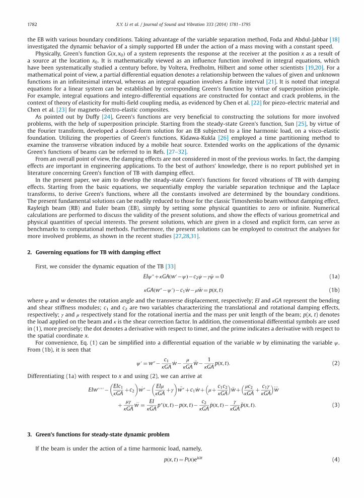
Fig. 6. Dimensionless Green's functions Ψ ðξ;1=2Þ of EB, RB and TB corresponding to different dimensionless frequencies Ω1 ¼ 0:5(a) and Ω1 ¼ 5:0(b) ofexternal dynamic force.

X.Y. Li et al. / Journal of Sound and Vibration 333 (2014) 1781–17951792

those for EB, which indicates that the rotational inertia has weak influence on the deflections. On the other hand, theamplitudes of TB are much larger than those for RB and TB. This means that the shear effect introduce in TB model has asignificant influence on the vibration of the beam. As shown in Fig. 6, the similar observation is found in the variable ψ ,which is consistent with the conclusion drawn by Ref. [29]. As shown in Fig. 6, there is a discontinuity in Ψ ðξ;1=2Þ at ξ¼ 0:5in TB model, where the shear effect is taken into account.

6.4. Effect of damping factors

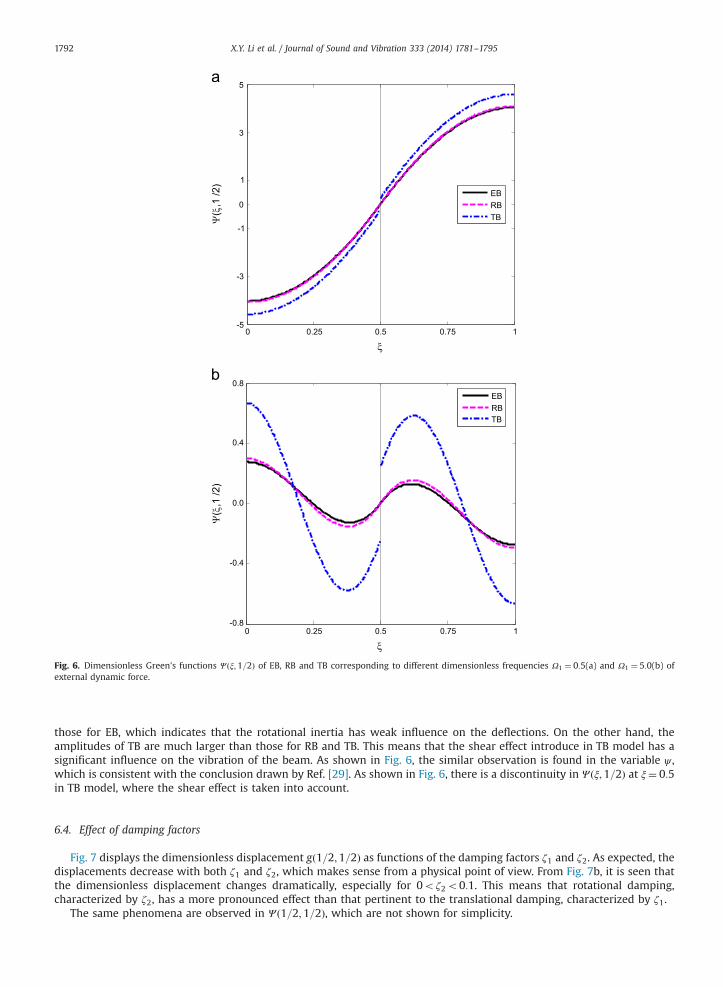
Fig. 7 displays the dimensionless displacement gð1=2;1=2Þ as functions of the damping factors ζ1 and ζ2. As expected, thedisplacements decrease with both ζ1 and ζ2, which makes sense from a physical point of view. From Fig. 7b, it is seen thatthe dimensionless displacement changes dramatically, especially for 0oζ2o0:1. This means that rotational damping,characterized by ζ2, has a more pronounced effect than that pertinent to the translational damping, characterized by ζ1.

The same phenomena are observed in Ψ ð1=2;1=2Þ, which are not shown for simplicity.

0 0.25 0.5 0.75 1-1.6

-1.2

-0.8

-0.4

0.0

1

g(1/

2,1/

2)

2=0.0

2=0.5

2=1.0

0 0.25 0.5 0.75 1-1.6

-1.2

-0.8

-0.4

0.0

2

g(1/

2,1/

2)

1=0.0

1=0.5

1=1.0

Fig. 7. The dimensionless deflection g 1=2;1=2�

of TB as functions of the damping ratio ζ1 (a) and ζ2 (b).

X.Y. Li et al. / Journal of Sound and Vibration 333 (2014) 1781–1795 1793

7. Conclusions

In this paper, forced vibration of a Timoshenko beam with various boundary conditions is systematically studied by virtueof Laplace transform. Corresponding Green's functions, which can be readily degenerated to Euler and Rayleigh beams, areexplicitly presented in terms of elementary functions. The effects of various important parameters are numerically examined.

The validity of the present solutions is discussed in both analytical and numerical ways. The results, which aredegenerated from the present solutions, are identical to those developed by Abu-Hilal [17]. To further validate the presentsolutions, comparison has been numerically made with those predicted by [15] and those exacted from FEM. Numericalresults clearly reveals that the difference between the present result and its counterpart are smaller than 5 percent, which isdifficult to be investigated in engineering applications.

In the study of forced vibration, Timoshenko beam model, instead of Euler and Rayleigh beams, should be employed for abeam with a height-to-length larger than 0.10. This is consistent with the observation for static problems. In particular, therotational damping has a larger influence on the steady response of the beam than the translational damping.

X.Y. Li et al. / Journal of Sound and Vibration 333 (2014) 1781–17951794

It should be mentioned that the present analysis focuses on the forced vibration of Timoshenko beams with dampingeffects. Vibrations coupling bending and torsion are beyond the scope of the present paper. Under such a circumstance, thegoverning equation is of nonlinear nature, which would be an interesting topic in the future studies.

The present Green's functions may be applied to constructing much more involved problems. For instance, the presentmethod can be extended to the field of vibration monitoring to evaluate the structural health of a cracked beam, by adoptingcorresponding model, as suggested by Dimarogonas [43] and Chondros and Dimarogonas [44]. Moreover, applications of thepresent solutions to discontinuous beams [27,28,31] or other disciplines such as biomechanics [45] can be expected as well.

Acknowledgments

The work was supported by the National Natural Science Foundation of China (Nos.11102171, 11072204 and 11372257)and Program for New Century Excellent Talents in University of Ministry of Education of China (NCET-13–0973).The supports from Sichuan Provincial Youth Science and Technology Innovation Team (2013), Scientific Research Foundationfor Returned Scholars (Ministry of Education of China) and the Fundamental Research Funds for the Central Universities(Nos: SWJTU11CX069 and SWJTU11ZT15) are acknowledged as well.

Appendix A

In this section, it is shown that the dimensionless Green's functions gðξ; ξ0Þ for simply supported EB defined in (28) isindependent of the height-to-length ratio β, as shown in Table 5.

Green's function G ξ; ξ0ð Þ for simply supported EB is identical to that in (21), with the constants W′ð0Þ and W‴ð0Þ specifiedby (20), and the functions ϕiðxÞði¼ 1;3;5Þ defined in (15). From these three equations, it is evident that Green's functionGðx; x0Þ is related to the constants a2 and b2 (bear in mind that a1 ¼ 0 and b1 ¼ 0 in this case as shown in Table 1).Furthermore the constant a2 can be put into the following form:

a2 ¼Ω2μ

EI¼Ω2

1Ω20μ

EI¼Ω2

1π

L

� �4 EIμ

μ

EI¼Ω2

1π

L

� �4(A.1)

which is independent of the height-to-length ratio β. As a result, the parameters siði¼ 1;2;…;4Þ and the functionsϕiðxÞði¼ 3;5Þ have nothing to do with β.

On the basis of these observations, we can rewrite Green's function for EB in the following form:

Gðx; x0Þ ¼ Gðx; x0Þb2 ¼Gðx; x0Þ

EI; (A.2)

where Gðx; x0Þ is independent of β. Consequently, the dimensionless Green's function gðξ; ξ0Þ can be transformed into

gðξ; ξ0Þ ¼ Gðx; x0Þ48EI

P0L3 ¼ Gðx; x0Þ

48

P0L3 (A.3)

which is evidently independent of the height-to-length ratio.

References

[1] V. Stojanović, P. Kozić, G. Janevski, Exact closed-form solutions for the natural frequencies and stability of elastically connected multiple beam systemusing Timoshenko and high-order shear deformation theory, Journal of Sound and Vibration 332 (2013) 563–576.

[2] G. Piccardo, F. Tubino, Dynamic response of Euler–Bernoulli beams to resonant harmonic moving loads, Structural Engineering and Mechanics 44 (2012)681–704.

[3] Z. Hryniewicz, Dynamics of Rayleigh beam on nonlinear foundation due to moving load using adomian decomposition and coiflet expansion, SoilDynamics and Earthquake Engineering 31 (2011) 1123–1131.

[4] W.R. Chen, Closed-form solutions on bending of cantilever twisted Timoshenko beams under various bending loads, Structural Engineering andMechanics 35 (2010) 261–264.

[5] M. Ghommem, A. Abdelkefi, A.O. Nuhait, M.R. Hajj, Aeroelastic analysis and nonlinear dynamics of an elastically mounted wing, Journal of Sound andVibration 331 (2012) 5774–5787.

[6] L. Wang, X. Guo, The wind–vehicle–bridge coupling dynamic analysis of three tower suspension bridge, Journal of Railway Science and Engineering 9(2012) 24–29.

[7] S.Y. Lee, Y.C. Cheng, A new dynamic model of high-speed railway vehicle moving on curved tracks, Journal of Vibration and Acoustics 130 (2008) 1–1010.[8] S.R. Chen, C.S. Cai, Equivalent wheel load approach for slender cable-stayed bridge fatigue assessment under traffic and wind: feasibility study, Journal

of Bridge Engineering 12 (2007) 755–764.[9] S.P. Brady, E.J. O'Brien, A. Znidaric, Effect of vehicle velocity on the dynamic amplification of a vehicle crossing a simply supported bridge, Journal of

Bridge Engineering 11 (2006) 241–249.[10] W.T. Thomson, Theory of Vibration with Applications, Prentice Hall, Englewood Cliffs, NJ, 1993.[11] W. Weaver Jr., S.P. Timoshenko, D.H. Young, Vibration Problems in Engineering, John Wiley & Sons, New York, 1990.[12] T.J. Levy, E. Rabani, Steady state conductance in a double quantum dot array: the nonequilibrium equation-of-motion Green's function approach,

Journal of Chemical Physics 138 (2013).[13] T. Sadi, J. Oksanen, J. Tulkki, P. Mattila, J. Bellessa, The Green's function description of emission enhancement in grated LED structures, IEEE Journal of

Selected Topics in Quantum Electronics 19 (2013).[14] A. Wacker, M. Lindskog, D.O. Winge, Nonequilibrium Green's function model for simulation of quantum cascade laser devices under operating

conditions, IEEE Journal of Selected Topics in Quantum Electronics 19 (2013).

X.Y. Li et al. / Journal of Sound and Vibration 333 (2014) 1781–1795 1795

[15] G.G.G. Lueschen, L.A. Bergman, D.M. McFarland, Green's functions for uniform Timoshenko beams, Journal of Sound and Vibration 194 (1996) 93–102.[16] S.M. Lin, S.Y. Lee, Closed-form solutions for dynamic analysis of extensional circular Timoshenko beams with general elastic boundary conditions,

International Journal of Solids and Structures 38 (2001) 227–240.[17] M. Abu-Hilal, Forced vibration of Euler–Bernoulli beams by means of dynamic Green functions, Journal of Sound and Vibration 267 (2003) 191–207.[18] M.A. Foda, Z. Abduljabbar, A dynamic Green function formulation for the response of a beam structure to a moving mass, Journal of Sound and

Vibration 210 (1998) 295–306.[19] D.L. Colton, R. Kress, Integral Equation Methods in Scattering Theory, Wiley, New York, 1983.[20] F.G. Tricomi, Integral Equations, Courier Dover, New York, 1957.[21] A. Myskis, Advanced Mathematics for Engineers, Mir Publishers, Moscow, 1975.[22] W.Q. Chen, T. Shioya, H.J. Ding, Integral equations for mixed boundary value problem of a piezoelectric half-space and the applications, Mechanics

Research Communications 26 (1999) 583–590.[23] W.Q. Chen, E.N. Pan, H.M. Wang, C.Z. Zhang, Theory of indentation on multiferroic composite materials, Journal of the Mechanics and Physics of Solids

58 (2010) 1524–1551.[24] D.G. Duffy, Green's Functions with Applications, Chapman and Hall/CRC, New York, 2001.[25] L. Sun, A closed-form solution of a Euler–Bernoulli beam on a viscoelastic foundation under harmonic line loads, Journal of Sound and Vibration 242

(2001) 619–627.[26] J. Kidawa-Kukla, Application of the Green's functions to the problem of the thermally induced vibration of a beam, Journal of Sound and Vibration 262

(2003) 865–876.[27] S. Caddemi, I. Caliò, F. Cannizzaro, Closed-form solutions for stepped Timoshenko beams with internal singularities and along-axis external supports,

Archive of Applied Mechanics (2013) 1–19.[28] G. Failla, Closed-form solutions for Euler–Bernoulli arbitrary discontinuous beams, Archive of Applied Mechanics 81 (2011) 605–628.[29] L. Majkut, Free and forced vibrations of Timoshenko beams described by single difference equation, Journal of Theoretical and Applied Mechanics 47

(2009) 193–210.[30] B. Mehri, A. Davar, O. Rahmani, Dynamic Green's function solution of beams under a moving load with different boundary conditions, Scientia Iranica

16 (2009) 273–279.[31] G. Failla, A. Santini, On Euler–Bernoulli discontinuous beam solutions via uniform-beam Green's functions, International Journal of Solids and Structures

44 (2007) 7666–7687.[32] S. Kukla, I. Zamojska, Frequency analysis of axially loaded stepped beams by Green's function method, Journal of Sound and Vibration 300 (2007)

1034–1041.[33] E. Manoach, P. Ribeiro, Coupled, thermoelastic, large amplitude vibrations of Timoshenko beams, International Journal of Mechanical Sciences 46 (2004)

1589–1606.[34] V.A. Ditkin, A.P. Prudnikov, Formulaire Pour le calcul Opérationnel, Masson Cie, Paris, 1967.[35] S. Timoshenko, Strength of Materials, D. Van Nostrand Company, New York, 1930.[36] R.E.D. Bishop, D.C. Johnson, The Mechanics of Vibration, Cambridge University Press, Cambridge, 2011.[37] N.E. Huang, Z. Shen, S.R. Long, M.C. Wu, H.H. Shih, Q. Zheng, N.-C. Yen, C.C. Tung, H.H. Liu, , The empirical mode decomposition and the Hilbert

spectrum for nonlinear and non-stationary time series analysis, Proceedings of the Royal Society of London. Series A: Mathematical, Physical andEngineering Sciences, 454 (1998) 903-995.

[38] J. Hutchinson, Shear coefficients for Timoshenko beam theory, Journal of Applied Mechanics of the ASME 68 (2001) 87–92.[39] Y.K. Cheung, D. Zhou, Vibrations of moderately thick rectangular plates in terms of a set of static Timoshenko beam functions, Computers & Structures

78 (2000) 757–768.[40] T. Kaneko, On Timoshenko's correction for shear in vibrating beams, Journal of Physics D: Applied Physics 8 (1975) 1927.[41] S.P. Timoshenko, On the correction for shear of the differential equation for transverse vibrations of prismatic bars, Philosophical Magazine 41 (1921)

744–746.[42] T.C. Huang, The effect of rotatory inertia and of shear deformation on the frequency and normal mode equations of uniform beams with simple end

conditions, Journal of Applied Mechanics of the ASME 28 (1961) 579–584.[43] A.D. Dimarogonas, Vibration of cracked structures: a state of the art review, Engineering Fracture Mechanics 55 (1996) 831–857.[44] T. Chondros, A. Dimarogonas, Influence of cracks on the dynamic characteristics of structures, Journal of Vibration, Acoustics, Stress and Reliability in

Design 111 (1989) 251–256.[45] I. Goda, M. Assidi, S. Belouettar, J.F. Ganghoffer, A micropolar anisotropic constitutive model of cancellous bone from discrete homogenization, Journal

of the Mechanical Behavior of Biomedical Materials 16 (2012) 87–108.