greenhouse gas emissions from beef...

4

GREENHOUSE GAS EMISSIONS FROM BEEF CATTLE GRAZING SYSTEMS IN FLORIDA

By

MARTA MOURA KOHMANN

A THESIS PRESENTED TO THE GRADUATE SCHOOL

OF THE UNIVERSITY OF FLORIDA IN PARTIAL FULFILLMENT OF THE REQUIREMENTS FOR THE DEGREE OF

MASTER OF SCIENCE

UNIVERSITY OF FLORIDA

2013

2

© 2013 Marta Moura Kohmann

3

To God, the best Agricultural Engineer I know, and to my family

4

ACKNOWLEDGMENTS

I would like to start thanking God for giving me a very long list of people for

which to be thankful. First of all, I would like to thank my wonderful family for the love

and encouragement they gave me even from a distance. Thanks to my parents for

helping with words of wisdom and inspiration and for helping me keep my feet on the

ground. To my siblings, thank you for listening to me and making me laugh. To the

Turma in Porto Alegre, thank you for the unconditional support. Second, I would like

to thank Dr. Clyde W. Fraisse, my committee chair, for the outstanding guidance

through my Master’s program and for being an example of how leadership,

innovation and interdisciplinary work can achieve great accomplishments. I would

like to express my deep appreciation for the crucial help of Dr. DiLorenzo and Dr.

Sollenberger in designing and performing the field experiment. I would also like to

thank Dr. Adesogan and Dr. Asseng for the insights and direction through this

process. My most sincere gratitude is extended to Francine Messias Ciríaco Silva,

Darren D. Henry, Martin Ruiz Moreno, Miquéias Barbosa and to everyone at the

North Florida Research and Education Center, Marianna for their help with the field

and laboratory measurements. Thanks for keeping good spirits in the hot Florida

summer! I would also like to thank the AgroClimate Team (Verona Oliveira Montone,

Eduardo Gelcer, José Henrique Debastiani Andreis, Tiago Zortea, Ana Paula Luz

Wagner, Carlos Torres, Hermes Cuervo and Daniel R. Dourte). We faced many

challenges together and I am glad I had your friendship to encourage me. I would

like to thank my gaucho family (Marcelo Osório Wallau, Alisson Pacheco Kovaleski

and Bruno Casamali), for being available to share companionship and mate. I am

also very grateful to my American family: to Monica Moss, Cameron and Bryant

Seamon, Ginger Meyers and their families who “adopted” me. Finally, my gratitude

5

to UFRGS for providing me great, free education. I would like to thank particularly Dr.

Moacir Antonio Berlato (and the Agromet group) and Dr. Paulo César de Faccio

Carvalho (and the Grupo de Estudo de Ecologia em Pastejo) for first introducing me

to research and for inspiring me to always ask questions and work hard.

6

TABLE OF CONTENTS page

ACKNOWLEDGMENTS .................................................................................................. 4

LIST OF TABLES ............................................................................................................ 8

LIST OF FIGURES ........................................................................................................ 10

ABSTRACT ................................................................................................................... 13

CHAPTER

1 CARBON FOOTPRINT ESTIMATION .................................................................... 15

Literature Review .................................................................................................... 15 Materials and Methods............................................................................................ 18

Site Description ................................................................................................ 18

Identification of GHG Sources .......................................................................... 19

Equations ......................................................................................................... 21 Enteric fermentation ................................................................................... 21

Manure ....................................................................................................... 24 Burning of pasture ...................................................................................... 28

Nitrogen fertilizer ........................................................................................ 28 Lime ........................................................................................................... 30

Emissions during production, transportation, storage and transfer ............ 31 Feed concentrate ....................................................................................... 31 Fuel ............................................................................................................ 32

Results .................................................................................................................... 32 Discussion .............................................................................................................. 33

Conclusions ............................................................................................................ 37

2 SENSITIVITY ANALYSIS OF ENTERIC FERMENTATION EMISSION MODEL ................................................................................................................... 49

Literature Review .................................................................................................... 49 Materials and Methods............................................................................................ 53

Model................................................................................................................ 53

Data Source ..................................................................................................... 56 Vary-one-at-a-time (OAT) ................................................................................. 57 Morris ............................................................................................................... 57 FAST ................................................................................................................ 59

Results .................................................................................................................... 60

Discussion .............................................................................................................. 61 Conclusions ............................................................................................................ 67

3 RUMINAL METHANE EMISSIONS, FORAGE AND ANIMAL PERFORMANCE RESPONSES TO DIFFERENT STOCKING RATES ON CONTINUOUSLY STOCKED BAHIAGRASS PASTURES ..................................... 80

Literature Review .................................................................................................... 80

7

Materials and Methods............................................................................................ 88 Experimental Site ............................................................................................. 88 Treatments and Design .................................................................................... 89 Pasture and Animal Management .................................................................... 89

Ruminal Methane Emissions Measurements ................................................... 92 Statistical Analysis ............................................................................................ 94

Results .................................................................................................................... 94 Discussion .............................................................................................................. 94 Conclusions ............................................................................................................ 99

LIST OF REFERENCES ............................................................................................. 112

BIOGRAPHICAL SKETCH .......................................................................................... 121

8

LIST OF TABLES

Table page 1-1 Concentration of GHG in the atmosphere before the Industrial Revolution

and in 2005. Source: IPCC, 2007a. .................................................................... 38

1-2 Emission of greenhouse gases by economic sector, million metric tons CO2e. Source: EPA, 2013a. ............................................................................... 39

1-3 Emissions of GHG Agriculture in the USA (Tg CO2e year-1), 1990 to 2011. Source: EPA, 2013a. .......................................................................................... 40

1-4 Herd information from Buck Island Ranch (BIR), period 1998 to 2008. .............. 41

1-5 Area burned (ha) on Buck Island Ranch (BIR), period between 1998 and 2008. .................................................................................................................. 41

1-6 Average above ground biomass available for burning in Buck Island Ranch (BIR), average from period 1998 to 2008. ............................................... 41

1-7 Lime, fertilizer, molasses, feed concentrate and fuel used at Buck Island Ranch (BIR), 1998 to 2008. ................................................................................ 42

1-8 Source categories and GHG emitted in the production system at in Buck Island Ranch (BIR), 1998 to 2008. ..................................................................... 43

1-9 Global Warming Potential (GWP) of GHG. ......................................................... 43

1-10 Data and emissions factor values, units and sources. ........................................ 44

1-11 Data and emissions factor values, units and sources (continuation). ................. 45

2-1 Default values for parameters not evaluated in sensitivity analysis. ................... 68

2-2 Digestible energy (DE, %) and methane conversion rate (Ym, %) values and sources used in the sensitivity analyses. ..................................................... 69

2-3 Average daily gain (ADG, kg/day) values and sources used in the sensitivity analyses. ............................................................................................ 69

2-4 OAT, FAST and Morris indexes for the enteric fermentation emission model (IPCC, 2006). ADG = average daily gain, kg animal-1 day-1; DE = digestible energy, %; Ym = methane conversion rate, %. .................................. 70

2-5 Ranking of parameters' influence in the output of IPCC’s (2006) enteric fermentation model. ............................................................................................ 70

3-1 Soil types in experimental sites A and B. Source: USDA, 2013........................ 101

3-2 Herbage mass double sample regression equations. Period 1: 25 June to 22 July; Period 2: 23 July to 19 Aug.; Period 3: 20 Aug to 18 Sep. .................. 101

9

3-3 Effect of stocking rate (1.2, 2.4 and 3.6 AU ha-1) on response variables in 2012 period and treatment x period interaction on experimental variables. ...... 101

3-4 Forage herbage mass (HM) (kg ha-1) and herbage accumulation rate (HAR) (kg ha-1 day-1) response to three stocking rates (1.2, 2.4 and 3.6 AU ha-1) in 2012. Period 1: June 25 to July 22; Period 2: July 23 to Aug. 19; Period 3: Aug.20 to Sep. 18. ....................................................................... 102

3-5 Forage chemical composition response given by CP (%), NDF (%) and ADF(%) to three stocking rates (1.2, 2.4 and 3.6 AU ha-1) in 2012. Period 1: June 25 to July 22; Period 2: July 23 to Aug. 19; Period 3: Aug.20 to Sep. 18. ............................................................................................................ 102

3-6 Average daily gain (ADG, kg animal-1day-1), BW (kg animal-1), DMI (kg animal-1day-1) and DMI (kg BWl-1 day-1) response to three stocking rates (1.2, 2.4, 3.6 AU ha-1) in 2012. Period 1: June 25 to July 22; Period 2: July 23 to Aug. 19; Period 3: Aug.20 to Sep. 18. ..................................................... 103

3-7 Response of CH4 emissions expressed as g CH4 day-1, g kg BW-1 and g kg DMI-1 to three stocking rates (1.2, 2.4 and 3.6 AU ha-1) in 2012. Period 1: June 25 to July 22; Period 2: July 23 to Aug. 19; Period 3: Aug.20 to Sep. 18. ............................................................................................................ 104

10

LIST OF FIGURES

Figure page 1-1 Map of the state of Florida. "A" refers to the location of Buck Island Ranch

(BIR). .................................................................................................................. 46

1-2 Calendar of animals' reproductive stage. ............................................................ 46

1-3 Emissions from BIR, ton CO2e year-1. ................................................................ 47

1-4 GHG emissions from BIR per category, % over average of all years, 1998 to 2008. .............................................................................................................. 48

1-5 Average GHG emissions from synthetic N fertilizer and lime before and after they are applied on the farm. ...................................................................... 48

2-1 OAT experimental design used in the sensitivity analysis. ................................. 71

2-2 Evolution of the experimental design in Morris sensitivity analysis (a through c) for the parameters’ intervals in the pasture’s evaluation. ................... 72

2-3 Experimental design in the FAST method for animals on pasture and on feedlot. ADG= average daily gain, kg animal-1 day-1; DE= digestible energy, %; Ym= methane conversion rate, %. ................................................... 73

2-4 Experimental design in the FAST sensitivity analysis. ADG = average daily gain, kg animal-1 day-1; DE = digestible energy, %; Ym = methane conversion rate, %. ............................................................................................. 74

2-5 Output of enteric fermentation methane emission model (IPCC, 2006) in kg CH4 animal-1 year-1 as a function of parameter values in the OAT sensitivity analysis method. ................................................................................ 75

2-6 OAT index for sensitivity analysis of simulations on pasture and feedlot situations. ........................................................................................................... 76

2-7 FAST indexes for the enteric fermentation emission model (IPCC, 2006). ADG = average daily gain, kg animal-1 day-1; DE = digestible energy, %; Ym = methane conversion rate, %. .................................................................... 77

2-8 Morris indexes for the enteric fermentation emission model (IPCC, 2006). ADG = average daily gain, kg animal-1 day-1; DE = digestible energy, %; Ym = methane conversion rate, %. .................................................................... 78

2-9 Energy partitioning in animals. Adapt from: (Minson, 1990, Van Soest, 1982). ................................................................................................................. 79

2-10 Relationship between ADG (kg animal-1 day-1) and methane production (g CH4 ADG-1) for simulations made with Tier 2 enteric fermentation model (IPCC, 2006) for animals on pasture and feedlot................................................ 79

11

3-1 Map of experimental sites A and B located at the North Florida Research and Education Center (NFREC), Marianna, Florida. ........................................ 105

3-2 Animal with CH4 collection device. A: capillary tube placed on halter; B: collecting canister. Picture by Marta Moura Kohmann, 2012. ........................... 105

3-3 Herbage mass (kg ha-1) response to three stocking rates (1.2, 2.4 and 3.6 AU ha-1) in 2012. Period 1: June 25 to July 22; Period 2: July 23 to Aug. 19; Period 3: Aug.20 to Sep. 18. ....................................................................... 106

3-4 Herbage accumulation rate (HAR) (kg ha-1 day-1) i response to three stocking rates (1.2, 2.4 and 3.6 AU ha-1) in 2012. Period 1: June 25 to July 22; Period 2: July 23 to Aug. 19; Period 3: Aug. 20 to Sep. 18. ................ 106

3-5 Dry matter intake (DMI) (kg animal-1 day-1) response to three stocking rates (1.2, 2.4 and 3.6 AU ha-1) in 2012. Period 1: June 25 to July 22; Period 2: July 23 to Aug. 19; Period 3: Aug.20 to Sep. 18. ............................... 107

3-6 Dry matter intake (DMI) per kg body weight (BW) (kg kg-1 day-1) response to three stocking rates (1.2, 2.4 and 3.6 AU ha-1) in 2012. Period 1: June 25 to July 22; Period 2: July 23 to Aug. 19; Period 3: Aug.20 to Sep. 18. ........ 107

3-7 Average daily gain (ADG) (kg animal-1 day-1) response to three stocking rates (1.2, 2.4 and 3.6 AU ha-1) in 2012. Period 1: June 25 to July 22; Period 2: July 23 to Aug. 19; Period 3: Aug.20 to Sep. 18. ............................... 108

3-8 Acid detergent fiber (ADF) (%) response to three stocking rates (1.2, 2.4 and 3.6 AU ha-1) in 2012. Period 1: June 25 to July 22; Period 2: July 23 to Aug. 19; Period 3: Aug.20 to Sep. 18. .......................................................... 108

3-9 Neutral detergent fiber (NDF) (%) response to three stocking rates (1.2, 2.4 and 3.6 AU ha-1) in 2012. Period 1: June 25 to July 22; Period 2: July 23 to Aug. 19; Period 3: Aug.20 to Sep. 18. ..................................................... 109

3-10 Crude protein (CP) (%) response to three stocking rates (1.2, 2.4 and 3.6 AU ha-1) in 2012. Period 1: June 25 to July 22; Period 2: July 23 to Aug. 19; Period 3: Aug.20 to Sep. 18. ....................................................................... 109

3-11 Methane production (g CH4 animal-1 day-1) response to three stocking rates (1.2, 2.4 and 3.6 AU ha-1) in 2012. Period 1: June 25 to July 22; Period 2: July 23 to Aug. 19; Period 3: Aug.20 to Sep. 18. ............................... 110

3-12 Methane production (g CH4 kg BW-1) response to three stocking rates (1.2, 2.4 and 3.6 AU ha-1) in 2012. Period 1: June 25 to July 22; Period 2: July 23 to Aug. 19; Period 3: Aug.20 to Sep. 18. .............................................. 110

3-13 Methane production (g CH4 kg DMI-1) response to three stocking rates (1.2, 2.4 and 3.6 AU ha-1) in 2012. Period 1: June 25 to July 22; Period 2: July 23 to Aug. 19; Period 3: Aug.20 to Sep. 18. .............................................. 111

3-14 Measured and simulated methane production (g CH4 animal-1 day-1) in three stocking rates (1.2, 2.4 and 3.6 AU ha-1) in 2012. The value for

12

IPCC Tier 1 is a default value for beef cattle in the United States (IPCC, 2006), while values for IPCC Tier 2 were simulated using the IPCC’s Tier 2 methodology (IPCC, 2006) using the average daily gain from Periods 1 and 3 in the field experiment presented in this chapter (Table 3-6). Period 1: June 25 to July 22; Period 2: July 23 to Aug. 19; Period 3: Aug.20 to Sep. 18. ............................................................................................................ 111

13

Abstract of Thesis Presented to the Graduate School of the University of Florida in Partial Fulfillment of the

Requirements for the Degree of Master of Science

GREENHOUSE GAS EMISSIONS FROM BEEF CATTLE GRAZING SYSTEMS IN FLORIDA

By

Marta Moura Kohmann

December 2013

Chair: Clyde W. Fraisse Major: Agricultural and Biological Engineering

Pastoral systems are of crucial importance for the economy of Florida. The

cattle industry in this state is composed mostly of cow-calf operations that rely

heavily on grazing systems using tropical grass species such as bahiagrass

(Paspalum notatum Flugge). Agricultural operations are also an important source of

greenhouse gas (GHG) emissions. Although the scientific community, governmental

organizations and public opinion have increased their interest in environmental

issues related to the production of food, little is known about the emission of GHG

from beef cattle in Florida. The objectives of this study were to estimate GHG

emissions (carbon footprint) from a typical low- input cow-calf operation in Florida,

examine the model used for estimation of animal methane (CH4) production and

measure animal CH4 production using the sulfur hexafluoride (SF6) tracer technique.

The model developed by IPCC with emission factors specific for the USA or Florida

was used when available from EPA. The greatest source of GHG in the cow- calf

operation studied was from enteric fermentation followed by manure. A sensitivity

analysis of the model used for estimating enteric CH4 production was performed with

Morris, Fourier Amplitude Sensitivity Test and the vary- one- at- a- time

methodologies. All analysis showed that average daily gain was the most important

factor influencing the model’s output for growing animals independent of feed. A field

14

experiment was carried out with three stocking rates (1.2, 2.4 and 3.6 AU ha-1) of

animals grazing bahiagrass. Forage quantity and nutritive value were measured, as

well as animal performance. Production of CH4 was measured using the SF6

technique. No effect of treatment was found in CH4 emissions or in other animal

variables. Emissions averaged 393 g CH4 animal-1 day-1. This was the first CH4

measurements for grazing beef cattle in Florida. Based on our results the IPCC Tier

2 and Tier 1 approaches seem to underestimate emissions of CH4 by grazing cattle,

with values of 121 and 145 g CH4 animal-1 day-1, respectively. Due to the great

importance of agriculture in Florida’s economy, it is essential to obtain more

information about emissions from different agriculture-related sources. This

information may help not only to improve model use but also to provide a better

understanding of alternative management approaches that can reduce or avoid GHG

emissions.

15

CHAPTER 1 CARBON FOOTPRINT ESTIMATION

Literature Review

Changes in climate have become increasingly important to society. In 1998,

the United Nations Environmental Programme (UNEP) and the World Meteorological

Organization (WMO) instituted a scientific body responsible for reviewing scientific,

social, economic, and technical information regarding climate change, called

Intergovernmental Panel on Climate Change (IPCC). This scientific body is

composed of scientists from 195 countries and, because of its intergovernmental

character, produces policy-neutral reports. Among its publications, IPCC produces

reports to explain the scientific basis of changes in climate, provide information on

climate change risk management and adaptation strategies, and establish guidelines

for estimating greenhouse gas (GHG) emissions (IPCC, 2013). In the USA, these

guidelines are used by the Environmental Protection Agency (EPA) to estimate GHG

emissions on a national scale.

According to IPCC (2007a), climate change exists when there is a statistical

difference in the average or variability of a climate’s property that continues for a

decade or more, whether it be natural or originate from anthropogenic actions. There

are several factors pointing to the intensification of the greenhouse effect, among

which are the increase in air and ocean temperatures, sea level and snow and ice

melting (IPCC, 2007a).

Some of the climate modifying agents includes greenhouse gases (GHG),

aerosols, solar radiation and surface cover. These factors change the Earth’s energy

balance positively or negatively and the intensity of this modification is called

radiative forcing, measured in W m-2. Anthropogenic activities can be a source of

GHG such as carbon dioxide (CO2), methane (CH4), nitrous oxide (N2O) and

16

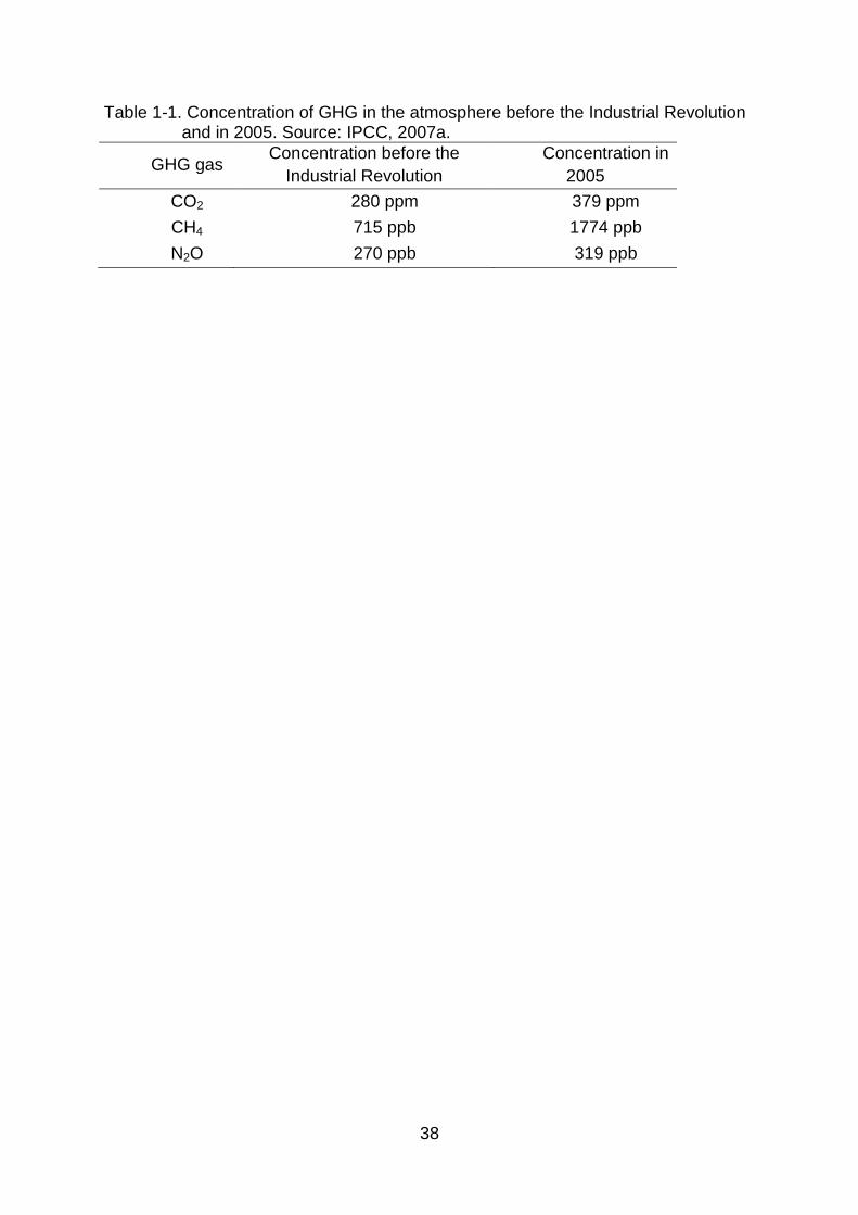
halocarbons. The concentrations of the first three before the Industrial Revolution

and in 2005 are presented in Table 1-1, where we can observe a significant increase

in their concentration in the atmosphere. Anthropogenic activities are estimated to

have had a positive radiative forcing in the order of 0.6 to 2.4 W m-2 since 1750

(IPCC, 2007a).

There are several sources of GHG related to human activities. In 2011, the

USA emitted 6,702 million metric tons of CO2 equivalent. Considering the carbon

sequestration occurring in land-use, land-use change and forestry in the US, net

emission was 5,797 million metric tons of CO2 equivalent in 2011. These emissions

were composed of different GHG, including 83.7% CO2, 8.8% CH4, 5.3% N2O and

2.2% HFC`s, PFC`s and SF6. Several economic sectors contribute to the GHG

emissions in the USA (Table 1-2). In 2011, agriculture contributed 6.9% of total

emissions in the USA (EPA, 2013a).

Agriculture is an important economic activity in Florida. In 2010, agricultural

products in Florida were worth 7.81 billion dollars, and cow-calf operations alone

accounted for 6.4% of this value. In fact, in January 2012 all cattle and calves in

Florida totaled 1,700,000 head, from which 940,000 were beef cattle. In 2011,

890,000 calves were born in Florida (Florida Department of Agriculture and

Consumer Services,2012). In this context, it is clear that assessing GHG emissions

from the beef industry in Florida is important, and the use of models is of particular

importance when analyzing production systems at both a farm scale (Beauchemin et

al., 2010) and at larger scales (Storm et al., 2012). Many studies have been

conducted regarding estimating GHG emissions from the processes involved in the

production of various produces. In fact, when searching for the term “carbon

footprint” in all scientific journals covered by ScienceDirect and Scopus, Wiedman

17

and Minx (2008) there were 42 hits of which 31 happened in 2007. Studying the

number of publications on Life Cycle Assessment (LCA) applied to agriculture

products between 2001 and 2011, Ruviaro et al. (2012) found a remarkable increase

in the number of studies produced particularly after 2007 probably related to

governmental and public inquiries regarding anthropogenic influence on global GHG

emissions.

The approach used to calculate the carbon footprint can vary greatly.

Although some authors define carbon footprint as the amount of CO2 solely emitted

directly and indirectly by an activity or through life stages of products (Wiedman and

Minx, 2008), the carbon footprint calculation for agriculture products usually accounts

for all of the different GHG involved in their production and transforms them into

CO2-equivalent (CO2e) according to each gas’ global warming potential (GWP)

(Röös et al., 2013). These estimations are important to identify the main sources of

GHG in a production system and point to possible areas of emission mitigation, as

well as energy use inefficiency (Lash and Wellington, 2007). With the increase of

society’s concern regarding environmental conservation, having to access

environmental records also presents a competitive advantage and can drive

purchase decisions (Lash and Wellington, 2007).

Considering the importance of cow-calf production in Florida and the

necessity to account for the GHG emissions related to this production system in

order to satisfy governmental and society’s inquiries regarding environmental

responsibility, the objective of this study was to quantify the carbon footprint of a

cow-calf operation in Florida.

18

Materials and Methods

Site Description

Buck Island Ranch (BIR) is located in Lake Placid, south-central Florida,

northwest of Lake Okeechobee (Figure 1-1). It has been managed by the Archbold

Biological Station since 1988 and, as a division of Archbold Expeditions, the

MacArthur Agro-ecology Research Center operates at BIR where it promotes long-

term ecological research (“Archbold Biological Station,” 2013). It also runs a

commercial cow-calf operation on an area of 4,200 ha, approximately 3000 Braham

cows and 250 Angus bulls (Table 1-4). Management makes use of natural service

during 5 to 7 months of the year (usually from January to May, but the breeding

season can be extended until June or July). Calves are born during the period of

November to March and are sold or transferred to other states at 7 months of age

(Figure 1-2). Approximately half of the grazing area is planted to bahiagrass, while

the other half is in semi-native pasture. The bahiagrass is occasionally managed with

burning.

According to Kottek et al. (2006), the climate in the region is classified as Cfa.

In this classification Cf stands for climates with warm temperatures and fully humid,

with minimum temperatures between -3 and 18 °C. The a refers to hot summers with

maximum temperatures above 22 °C. There are two soil types occurring the ranch.

They are classified as Felda fine sand, which is subjected to frequent flooding, and

Ona loamy sand where ground water levels vary between 25 and 100 cm throughout

the year (USDA, 1989).

Production records from 1998 to 2008 were considered in this case study.

According to the IPCC (2006) guidelines, GHG emissions can be estimated using

different levels of data and detail. The methodology used can be classified as Tier 1,

19

Tier 2 and Tier 3 to characterize increasing level of information needed to estimate

GHG emissions and accuracy of the predictions. The higher the Tier used, the

smaller the uncertainty.

Livestock categories to be considered in a GHG emission inventory should

include all of those which are important to a country or region. Category is described

as the animal species and it can be separated into subcategories according to age,

type of production and gender (IPCC, 2006). In this study the livestock category

considered was cattle, with three subcategories: cows, bulls and calves.

Identification of GHG Sources

The first step in calculating the carbon footprint of a production system

involves identifying the sources of GHG involved in the process. The source

categories and GHG emission considered in the calculation were identified according

to IPCC (2006), while considering specific emission factors available for Florida or

the USA in EPA (2013a; 2013b). The sources and GHG emitted at BIR in the period

of 1998 to 2008 are delineated in Table 1-8. A brief description follows.

Enteric fermentation. Enteric fermentation refers to a digestive process

where the anaerobic microbial population inside the animal’s digestive system

ferments feed and produces CH4 as a by-product. Ruminant livestock, including

cattle, sheep and goats, have greater rates of enteric fermentation because of their

unique digestive system, which includes a large rumen or fore-stomach where

enteric fermentation takes place. Production of CH4 depends on the animal’s

digestive system and quality and quantity of food (EPA, 2013a). IPCC (2006) only

considers emissions from animals older than 7 months of age.

Livestock waste. Manure can be managed in storage or treatment systems

or spread on fields in lieu of long-term storage or it can be deposited directly on

20

grazed lands. The management of livestock manure can produce CH4 and N2O.

Production of CH4 is a natural process in anaerobic decomposition of livestock

manure (EPA, 2013a). Emissions of N2O from livestock waste depend on the

composition of manure and urine, the type of bacteria involved in the process and

the amount of oxygen and water in the manure system. Direct N2O emissions are

produced as part of the N cycle through nitrification and denitrification of the organic

N in livestock manure or urine. Indirect N2O emissions are produced as result of the

volatilization of N as ammonia (NH3) and oxides of nitrogen (NOx) and runoff and

leaching of N during treatment, storage, and transportation (IPCC, 2006).

Pasture burning. Improved and native pastures in BIR are burned primarily

between December and February according to a burning schedule. Burns may

sometimes occur as late in the year as April in order to enhance biological diversity

including endangered and threatened species, reduce fire hazards, mimic natural

processes and provide educational and research opportunities (Main and Menges,

1997). When burning fields, CO2 is not considered to be released since it is largely

balanced by the CO2 that is reincorporated back into biomass via photosynthetic

activity within weeks or a few years after burning. Non-CO2 emissions, particularly

carbon monoxide (CO), CH4, N2O and other kinds of nitrogen oxides (NOx) that

result from incomplete combustion of biomass in managed grassland are reported

(IPCC, 2006). However, since there is no agreement regarding the GWP value and

signal for NOx, this gas was not considered in the evaluation (IPCC, 2006).

Fertilization (with synthetic fertilizer) and liming of pastures and crops.

Emissions from these processes include those from manufacturing, storage, transfer

and transportation as well as direct emissions of fertilizers and lime applied to the

field. The methodology used for accounting for manufacturing, storage and

21

transportation of fertilizers and lime was developed by Lal (2004). It estimates

carbon equivalent emissions by converting the energy or volume involved in the

production processes to kg of carbon equivalent (kg CE). After application to the

field, fertilizers also release N2O directly through the microbial processes of

nitrification and denitrification or indirectly by volatilization of ammonium (NH4+) and

nitrate (NO3-) or leaching and runoff mainly of nitrate, which can later go through

nitrification and denitrification (IPCC, 2006).

Tractor operations. This category includes all activities that require tractor

operations such as tilling, planting, harvesting, and application of agrochemicals.

These processes mostly release CO2, but also release CH4 and N2O. However, for

this paper the methodology used is that developed by the EPA (2005), which

considered only CO2 emissions based on the amount of carbon present in fuels.

Equations

Enteric fermentation

The first step necessary to calculate emissions from enteric fermentation is to

determine the different population subcategories. The total number of cows,

pregnancy rate, the number of calves and of bulls was obtained from the BIR

database. For the seven months after calving, we assumed that the number of

lactating cows equaled the number of calves. The cows pregnant in the next

breeding season were considered to be lactating. Remaining cows were considered

to be neither pregnant nor lactating. Therefore, there were five subcategories of

animals considered to emit CH4 from enteric fermentation: pregnant cows, lactating

cows, cows that were both pregnant and lactating, cows that were neither pregnant

nor lactating and bulls. Calves are not considered to emit CH4 from enteric

fermentation (IPCC, 2006).

22

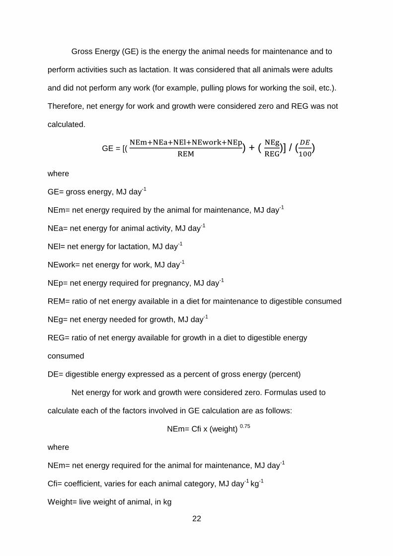
Gross Energy (GE) is the energy the animal needs for maintenance and to

perform activities such as lactation. It was considered that all animals were adults

and did not perform any work (for example, pulling plows for working the soil, etc.).

Therefore, net energy for work and growth were considered zero and REG was not

calculated.

GE = [(

) + (

)] / (

)

where

GE= gross energy, MJ day-1

NEm= net energy required by the animal for maintenance, MJ day-1

NEa= net energy for animal activity, MJ day-1

NEl= net energy for lactation, MJ day-1

NEwork= net energy for work, MJ day-1

NEp= net energy required for pregnancy, MJ day-1

REM= ratio of net energy available in a diet for maintenance to digestible consumed

NEg= net energy needed for growth, MJ day-1

REG= ratio of net energy available for growth in a diet to digestible energy

consumed

DE= digestible energy expressed as a percent of gross energy (percent)

Net energy for work and growth were considered zero. Formulas used to

calculate each of the factors involved in GE calculation are as follows:

NEm= Cfi x (weight) 0.75

where

NEm= net energy required for the animal for maintenance, MJ day-1

Cfi= coefficient, varies for each animal category, MJ day-1 kg-1

Weight= live weight of animal, in kg

23

NEl= Milk x (1.47+0.40 x Fat)

where

NEl= net energy for lactation, MJ day-1;

Milk= amount of milk produced, (kg of milk) day-1;

Fat= fat content of milk, % by weight.

NEp= Cpregnancy x NEm

where:

NEp= net energy required for pregnancy, MJ/day-1;

Cpregnancy= pregnancy coefficient;

NEm= net energy required for the animal for mantainance, MJ day-1. The NEm used

here was that considering pregnancy.

NEa= Ca x NEm

where

NEa= net energy for animal activity, MJ day-1;

Ca= activity coefficient corresponding to the animal’s feeding situation,

dimensionless;

NEm= net energy required for the animal for maintenance, MJ day-1.

REM= [1.123 - (4.092 x 10-3 x DE%) + [1.126 x 10-5 x (DE%)2] - (

)]

where

REM= ratio of net energy available in a diet for maintenance to digestible consumed;

DE= digestible energy expressed as a percentage of gross energy.

After the calculation of GE, a daily emission factor for each category was calculated

with the formula below.

24

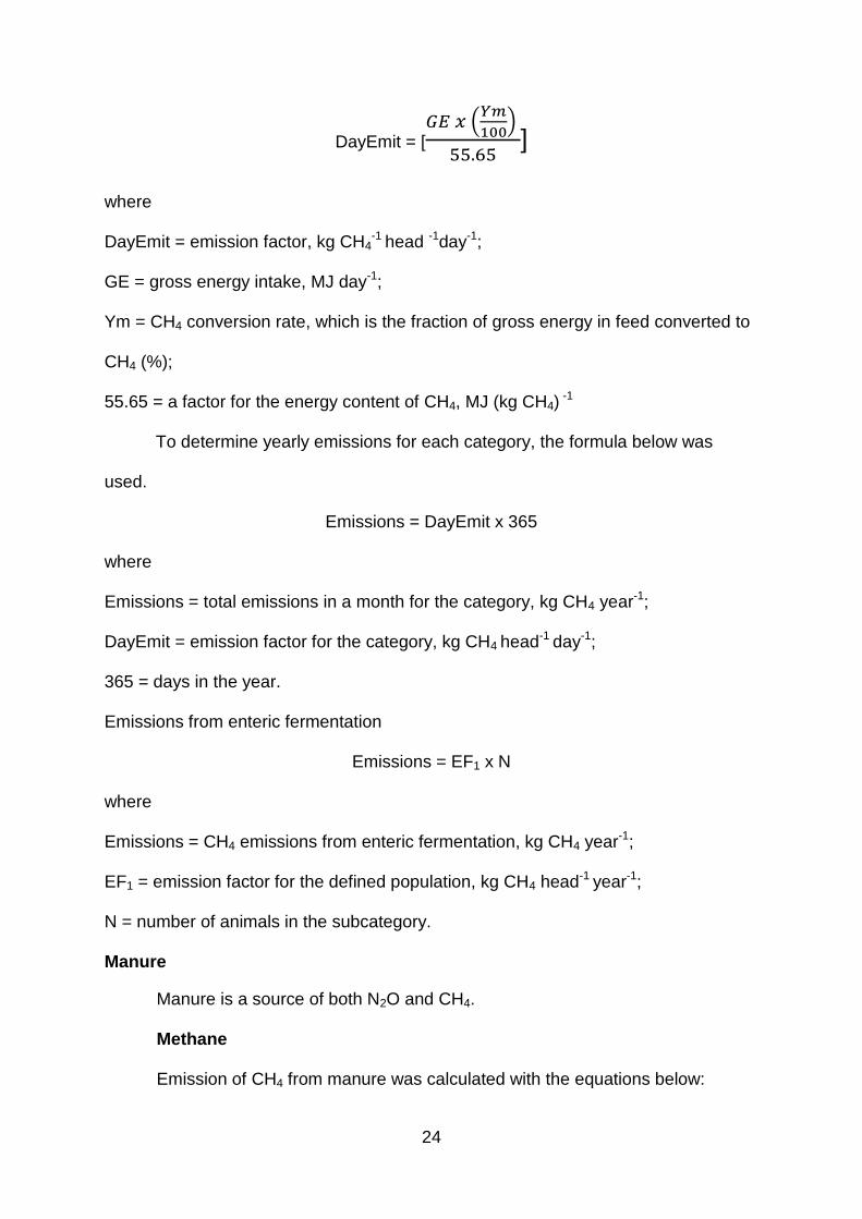
DayEmit = [ (

)

]

where

DayEmit = emission factor, kg CH4-1 head -1day-1;

GE = gross energy intake, MJ day-1;

Ym = CH4 conversion rate, which is the fraction of gross energy in feed converted to

CH4 (%);

55.65 = a factor for the energy content of CH4, MJ (kg CH4) -1

To determine yearly emissions for each category, the formula below was

used.

Emissions = DayEmit x 365

where

Emissions = total emissions in a month for the category, kg CH4 year-1;

DayEmit = emission factor for the category, kg CH4 head-1 day-1;

365 = days in the year.

Emissions from enteric fermentation

Emissions = EF1 x N

where

Emissions = CH4 emissions from enteric fermentation, kg CH4 year-1;

EF1 = emission factor for the defined population, kg CH4 head-1 year-1;

N = number of animals in the subcategory.

Manure

Manure is a source of both N2O and CH4.

Methane

Emission of CH4 from manure was calculated with the equations below:

25

EF(T) = VS(T) x [ Bo(T) x 0.67 x ∑S,k (MCFS,k/100) x MS(T,S,k)]

where

EF(T) = annual CH4 emission factor for category T, kg CH4 animal-1 year-1;

VS(T) = daily volatile solid excreted for category T, kg dry matter animal-1 year-1; for

calves, 210 days (7 months) were considered;

Bo(T) = maximum CH4 producing capacity for manure procedure by livestock

category T, m3 CH4 (kg of VS excreted)-1;

0.67 = conversion factor of m3 CH4 to kilogram CH4;

MCFS,k = CH4 conversion factors for each manure management system S by climate

region k, %;

MS(T,S,k) = fraction of livestock category T’s manure handled using manure

management system S in climate region k, dimensionless.

Nitrous oxide

N2O direct emissions

Direct N2O produced by the manure was calculated with the equations below.

N2Odirect = N2O-NPR = FPRP x EF3 PRP

where

N2Odirect –N = annual direct N2O-N emissions produced from livestock waste, kg

N2O-N year-1;

N2O-NPR = annual direct N2O-N emissions from urine and dung inputs to grazed

soils, kg N2O-N year-1;

FPRP = annual amount of urine and dung N deposited by grazing animals on pasture,

range and paddock, kg N year-1;

EF3 PRP = emission factor for N2O emissions from urine and dung N deposited on

pasture, range and paddock by grazing animals, kg N2O-N (kg N input)-1;

26

FPRP = [(N(T) x Nex(T)) x MS(T,PRP)]

where

N(T) = number of head of livestock species (category T)-1;

Nex(T) = annual average N excretion per head of species (category T)-1 (see Table 1-

7)

MS (T, PRP) = fraction of total annual N excretion for each livestock species (category

T)-1 that is deposited on pasture, range and paddock. It was considered 1 in this

case because all the excretion was deposited on pasture.

Nex(T) = EN x weight x days

where

Nex(T) = annual average N excretion per head of species (category T)-1;

EN = excretion of nitrogen, kg day-1 (1000 kg) -1;

weight = average animal weight during the period, kg;

days = number of days spent in the farm- 365 for cows and bulls and 210 for calves.

To convert the results from kg N2Odirect–N to kg N2O, the following formula was

used:

N2O = N2O–Ndirect x (44/28)

N2O indirect emissions

Indirect emissions of N2O have two sources calculated separately:

volatilization, and leaching and runoff.

To estimate volatilization, the following equation is used:

N2O(ATD) –N = [(FON + FPRP) x FracGASM)] x EF4

where:

N2O(ATD)– N = annual amount of N2O – N produced from atmospheric deposition of N

volatilized from managed soils, kg N2O – N year-1;

27

FON = annual amount of managed animal manure, compost, sewage sludge and

other organic N additions applied to soils, kg N year-1, considered zero in this

situation;

FPRP = annual amount of urine and dung N deposited by grazing animals on pasture,

range and paddock, kg N year-1. Same as the one used to calculate direct N2O

emissions from manure management;

FracGASM = fraction of applied organic N fertilizer material (FON) and of urine and

dung N deposited by grazing animals (FPRP) that volatilizes as NH4 and NO4, kg N

volatilized (kg of N applied or deposited) -1;

EF4 = emission factor for N2O emissions from atmospheric deposition of N on soils

and water surfaces, kg N2O – N (kg NH3-N + NOx-N)-1 volatilized.

To estimate leaching and runoff, the following equation was used:

N2O(L)– N = [(FON + FPRP) x FracLEACH– (H))] x EF5

where

N2O(L) –N = annual amount N2O –N produced from leaching and runoff of N additions

to managed soils in regions where leaching/runoff occurs, kg N2O –N year-1;

FracLEACH– (H) = fraction of all N added in regions where leaching/runoff occurs that is

lost through leaching and runoff, kg N (kg on N added)-1;

EF5 = emission factor for N2O emissions from N leaching and runoff, kg N2O –N (kg

N leached and runoff)-1.

After that, both N from volatilization and from leaching and runoff are

summed, as showed below.

N2Oindirect– N = N2O(L)– N + N2O(ATD)– N

where

28

N2Oindirect –N = annual indirect N2O-N emissions from urine and dung inputs to

grazed soils, kg N2O-N year-1.

To convert the results from kg N2Oindirect –N to kg N2O, the following formula

was used:

N2O = N2O–Nindirect x (44/28)

Burning of pasture

The equation used to estimate emissions from pasture burning is shown

below.

Lfire= A x MB x Cf x Gef x 10-3

where

Lfire= amount of GHG emissions from fire, tones of each GHG. Indirect GWP for CO

was considered 1.9 (IPCC, 2006);

A= area burnt, ha (Table 1-5);

MB= mass of fuel available for combustion, ton ha-1. It includes biomass, ground litter

and dead wood, but when using the Tier 1 method ground litter and dead wood are

considered zero except when there is land-use change. The average of above

ground mass available for all native or all improved pastures in a specific month was

used (Table 1-6).

Cf= combustion factor, dimensionless;

Gef= emission factor, g (kg dry matter burnt)-1.

Nitrogen fertilizer

After nitrogen fertilizers are applied to the soil, they release N2O directly and

indirectly, with the same methodology used to calculate N2O emissions from animal

waste.

Direct emissions

29

N2Odirect -N = N2Oimput = FSN x EF1

where

N2Odirect –N = annual direct N2O-N emissions produced from managed soils, kg N2O-

N year-1;

N2Oimput –N = annual direct N2O-N emissions from N inputs to managed soils, kg

N2O-N year-1;

N2Odirect –N = annual direct N2O-N emissions produced from managed soils, kg N2O-

N year-1;

N2Oimput –N = annual direct N2O-N emissions from N inputs to managed soils, kg

N2O-N year-1;

FSN = annual amount of synthetic fertilizer N applied to soils, kg N year-1;

EF1 = emission factor for N2O emissions from N inputs, kg N2O-N (kg N input) -1.

Indirect emissions

Similarly to manure management, indirect emissions from synthetic N fertilizer

application happened through volatilization, and leaching and runoff. To estimate

volatilization, the formula used was:

N2O(ATD)– N = FSN x FracGASF x EF4

where

N2O(ATD)– N = annual amount of N2O –N produced from atmospheric deposition of N

volatilized from managed soils, kg N2O– N year-1;


FracGASF = fraction of synthetic fertilizer N that volatilizes as NH3 and NOx, (kg N

volatilized) (kg N applied)-1;

EF4 = emission factor for N2O emissions from atmospheric deposition of N on soils

and water surfaces, kg N2O – N (kg NH3-N + NOx-N)-1 volatilized.

30

To estimate leaching and runoff, the formula used was:

N2O(L) –N = FSN x FracLEACH - (H) x EF5

where

N2O(L) –N = annual amount N2O –N produced from leaching and runoff of N additions

to managed soils in regions where leaching/runoff occurs, kg N2O–N year-1;


FracLEACH – (H) = fraction of all N added in regions where leaching/runoff occurs that is

lost through leaching and runoff, kg N (kg of N applied)-1;

EF5 = emission factor for N2O emissions from N leaching and runoff, kg N2O–N (kg N

leached and runoff)-1.

To estimate total indirect emissions from synthetic fertilizers, emissions from

leaching and runoff and volatilization were summed as shown below.

N2Oindirect– N = N2O(L)– N + N2O(ATD)– N

where

N2Oindirect –N = annual indirect N2O-N emissions from urine and dung inputs to

grazed soils, kg N2O-N year-1.

To convert the results from kg N2Oindirect –N to kg N2O, the following formula

was used:

N2O = N2O–Nindirect x (44/28)

Lime

The equation used to estimate the emission from lime (dolomite in this case)

after it was applied to the soil was:

CO2-C Emissions = (Mdolomite x EFdolomite)

CO2-C Emissions = annual carbon emissions from lime application, tones C year-1

Mdolomite = annual amount of calcic dolomite, tons year-1;

31

EFdolomite = emission factor, tons of CO2 (ton of dolomite lime)-1.

Emissions during production, transportation, storage and transfer

Off-farm emissions are an important source of GHG. Many steps are involved

before agrochemicals arrive at a farm or ranch. Lal (2004a) developed a

methodology to account for GHG emissions from production, transportation, storage

and transfer of agrochemicals. In this case study, these emissions are those related

to the use fertilizer and lime. For synthetic N fertilizer, the formula used was

Carbon emission = FSN x Equivalent Carbon Emission x (44/28) / 1000

where

Carbon emission = emissions, in kg CO2e year-1;


Equivalent Carbon Emission = C emission in relation to production, packaging,

storage and distribution of fertilizers, kg CE (kg N)-1.

For the emissions regarding lime’s production, transportation, storage and

transfer, the equation used was

Carbon emission = Mdolomite x Equivalent Carbon Emission x (44/28) / 1000

where

Carbon emission = emissions, in tons CO2e year-1;

Mdolomite = annual amount of synthetic fertilizer N applied to soils, kg year-1;

Equivalent Carbon Emission = C emission in relation to production, packaging,

storage and distribution of fertilizers, kg CE (kg N)-1.

Feed concentrate

For feed concentrate, the value of 780 kg CO2e t-1 of feed concentrate

according to Casey and Holden (2006). Amount of feed concentrate used is

presented on Table 1-7.

32

Fuel

The formula used to obtain CO2 emissions from gasoline and diesel used on

BIR is shown below. It was considered that the emissions from molasses should be

accounted for in sugarcane production and processing, so that emissions regarding

the use of molasses are only those ones related to transportation.

EmFuel = Fuel x Efuel

where

EmFuel= CO2e emissions, kg CO2 year-1;

Fuel= amount of fuel used, gallons year-1;

Efuel= emission factor, kg CO2e gallon-1.

After emissions were calculated they were expressed as CO2 equivalent

(CO2e) emitted per unit of live weight produced. The CO2e is a measure used to

compare the emissions from various greenhouse gases based upon their global

warming potential. For example, the global warming potential for CH4 over 100 years

is 25. This means that emissions of one metric ton of CH4 are equivalent to

emissions of 25 metric tons of CO2 (IPCC, 2007b).

Emission factors and other data used for calculating the emissions above

described are on Table 1-10 and Table 1-11. Production data including the use of

fertilizer, lime and fuel are on Table 1-7.

Results

Results from the carbon footprint calculation from BIR are shown in Figure 1-3

and Figure 1-4. On average, annual emissions in BIR were of 10,470 tons CO2e

year-1 and ranged from 8,750 tons CO2e year-1 in 1999 and 12,360 tons CO2e year-1

in 2004. The main source of GHG in this production system is enteric fermentation

(55 %), followed by animal waste (27 %), corresponding to 5,770 and 2,790 tons

33

CO2e year-1, respectively. Application of fertilizer and lime contribute on average with

11 % of total annual emissions in BIR.

In evaluating the variation in amount of GHG emitted yearly at BIR (Figure 1-

3) it is possible to determine that the amount of GHG from the main contributors to

total emissions (enteric fermentation and animal waste) did not show great

fluctuation from one year to the next. The variation observed, however, may be

related to the use of management practices such as pasture burning and application

of synthetic N fertilizer and lime. The emissions from the use of synthetic N fertilizer

and lime can be separated into on farm and pre-farm emission (Figure 1-5).

Emissions related to production, transportation, storage and transfer can be very

important when considering the use of agrochemicals. In fact, when looking at the

emissions from the use of N fertilizer alone, 43% of the GHG emissions occurred

before its use. The proportion of emissions occurring during production,

transportation, storage and transfer of lime is very significant and accounted for 71%

of total emissions connected to its utilization. In a more intensively managed system,

where liming and application of fertilizers may be more frequent, the pre-farm GHG

production should have greater importance than in the current case study.

The objective of production in BIR is weaned calves, which after 7 months of

age are sold or transferred to other regions of the US. Expressing GHG emissions as

a function of product originated in a production system can be a useful way to

compare different production systems. On average, 22.1 kg CO2e (kg calf LW)-1 was

emitted at BIR.

Discussion

In this case study, enteric fermentation was the largest contributor to total

GHG emissions in a cow-calf production system (Figure 1-4). This is in accordance

34

with other studies performed on GHG emissions from beef production systems.

Beauchemin et al. (2010) performed a Life Cycle Assessment (LCA) of beef

production in western Canada and found that 63% of emissions had their source in

enteric fermentation. In the same study, CH4 and N2O emissions from beef manure

accounted for 28% of total GHG emissions. These results are very similar to those

presented in this study, where 55% if emissions came from enteric fermentation and

27% from manure. Basarab et al. (2012) found that enteric fermentation was

responsible for 53 to 54% of total emissions when evaluating the full production cycle

of a beef herd. When analyzing different beef production systems in Ireland, Foley et

al. (2011) found that 46 to 53% of total emissions came from enteric fermentation. It

is important to notice that the emissions from enteric fermentation in this study are

not directly related to the production of meat since it mainly considers the adult cows.

In fact, the productive cows in a full- herd production cycle can account for up to 70%

of total GHG emissions (Basarab et al., 2012). Other authors have also highlighted

the relevance of GHG emissions coming from animals in the cow-calf production

phase, which require high levels of feed for maintenance and low production relative

to other production phases in the beef industry (Johnson et al., 2001a).

Management strategies can be used to decrease GHG emissions. The use of

growth implants, for example, can reduce the carbon footprint of beef production by

5% (Basarab et al., 2012). Feed management can also strongly influence the carbon

footprint. Animals fed high concentrate diets may have less energy lost as CH4

(Kurihara et al., 1999; Beauchemin and Mcginn, 2005), while low quality feed can

result in higher emissions from enteric fermentation (Phetteplace et al., 2001).

However, Yan et al. (2010) emphasized that at the farm level it is necessary to

consider several aspects associated with maintaining high level production animals

35

including emissions associated with soil management, feed production and use of

fertilizers. This is an important component of more intensively managed systems.

Although in this case study the amount of fertilizers and lime applied is not large, it is

crucial to acknowledge the importance of GHG emissions occurring before

application of these and other products. As Figure 1-5 shows, pre-farm emissions

can account for a considerable part of emissions related to the use of agrochemicals,

particularly for lime. Although the intensification of management practices can

increase total GHG emissions, it can also reduce emissions per unit of product.

When analyzing production scenarios varying in management practices in Ireland,

Foley et al. (2011) found that inputs required for higher production levels resulted in

higher carbon footprint when expressed as tons CO2e year-1. However, when

expressed as kg CO2e (kg beef)-1, high level production systems had a lower carbon

footprint because of associated improvements in fertilizer use and animal growth.

Basarab et al. (2012) highlight the fact that time is an important factor when

analyzing carbon footprint, particularly regarding the comparison of different

production systems. The authors affirm that expressing results of carbon footprint as

kg CO2e (kg beef)-1 can underestimate the disparity between carbon footprint if a

time correction is not made, since higher productivity can be associated with greater

animal production per unit of time.

Another relevant aspect of pasture- based production is the ability of the

pasture to fix atmospheric carbon (Soussana et al., 2004), and this was not

considered in this simulation. The use of pasture as animal feed has several

environmental advantages besides potentially reducing the carbon footprint of beef

production, including the decrease in emissions from manure and return of nutrients

to the soil and making use of the ruminants’ ability to convert high fiber material into

36

high quality protein (Beauchemin et al., 2010; Pelletier et al., 2010). If considering

carbon sequestration from pastures, carbon loss in annual cropping and land used in

the production of hay the carbon footprint in a beef production system was reduced

from 11 to 16% (Basarab et al., 2012). It has also been suggested that best

management practices such as intensifying the production system can decrease the

carbon footprint through carbon fixation by 15 to 30% while maintaining production

levels (Phetteplace et al., 2001).

Using a life cycle assessment (LCA) in western Canada, Beauchemin et al.

(2010) found that 83% of GHG emissions in the beef production chain of the region

originated in the cow-calf phase. In the US beef production system, the cow-calf

phase of beef production was found to be responsible for 76% of GHG emissions

(Johnson et al., 2001a). Calves leave BIR with an average weight of 210 kg and, on

average, GHG emissions per product are of 22 kg CO2e (kg calf LW)-1. This is in

agreement with a study performed in the US using information from Alabama,

Texas, Utah, Virginia and Wisconsin where GHG emissions per product were 21 kg

CO2e (kg calf LW)-1 (Phetteplace et al., 2001).

The studies conducted by Johnson et al. (2001a) and Beauchemin et al.

(2010) demonstrated that most of the GHG emissions in beef production systems

(76 and 83%, respectively) come from the cow-calf phase. However, most of the

weight gain of animals occurs after they leave the cow-calf phase. Therefore, when

expressing the carbon footprint per unit of beef produced as CO2 e (kg beef)-1, higher

values are found for the cow-calf phase than for the whole system. If we consider

that the animals leaving BIR may achieve 490 kg at slaughter and have 62% of this

weight as hot carcass (Miller et al., 1996), we find that emissions for the whole beef

production cycle would be of 12 kg CO2e (kg beef)-1 on a live weight basis or 19 kg

37

CO2e (kg beef)-1 on carcass weight basis. This agrees with many other studies

performed in similar production systems. In the US beef production system, the

emission of 13 to 16 CO2e (kg beef)-1 on a live weight basis was reported (Johnson

et al., 2001a), while Beauchemin et al. (2010) found 13 kg CO2e (kg beef)-1 on a live

weight basis and 22 kg CO2e (kg beef)-1 on a carcass weight basis in a case study

made for beef production in western Canada. Basarab et al. (2012) reported similar

values of 12 to 13 kg CO2e (kg beef)-1 on a live weight basis and 20 to 23 kg CO2e

(kg beef)-1 on a carcass weight basis. A range of 22 to 26 kg CO2e (kg beef)-1 on a

carcass weight basis was reported (Foley et al., 2011) for scenarios varying in feed

management in Ireland. In that study, Foley et al. (2011) found higher total emissions

in production systems with higher productivity and therefore input requirements.

However, this same scenario presented higher efficiency of fertilizer use and animal

performance, resulting in lower emissions relative to beef production. Production

efficiency is, therefore, an important aspect to consider when evaluating

management strategies to reduce carbon footprint. Expressing carbon footprint

relative to produce is a good indicative to production efficiency.

Conclusions

Emissions occurring on pre-farm (before use of specific products in the

system evaluated) are relevant and must be accounted for when assessing the

carbon footprint of agricultural production systems. In this case study, CH4 emissions

form enteric fermentation were the largest contributor to the carbon footprint.

Emissions from BIR varied from one year to another mostly because of management

practices such as lime and fertilizer application and pasture burning. On average,

BIR emitted 10,500 tons CO2e year-1 and 22 kg CO2e (kg calf LW)-1. These values

agree with other similar studies performed in the US and other developed countries.

38

Table 1-1. Concentration of GHG in the atmosphere before the Industrial Revolution and in 2005. Source: IPCC, 2007a.

GHG gas Concentration before the

Industrial Revolution

Concentration in

2005

CO2 280 ppm 379 ppm

CH4 715 ppb 1774 ppb

N2O 270 ppb 319 ppb

39

Table 1-2. Emission of greenhouse gases by economic sector, million metric tons CO2e. Source: EPA, 2013a.

Chapter/IPCC Sector 1990 2005 2007 2008 2009 2010 2011 2011 (%)

Energy 5,267.3 6,251.6 6,266.9 6,096.2 5,699.2 5,889.1 5,745.7 85.7

Industrial Processes 316.1 330.8 347.2 318.7 265.3 303.4 326.5 4.9

Solvent and Other Product Use

4.4 4.4 4.4 4.4 4.4 4.4 4.4 0.1

Agriculture 413.9 446.2 470.9 463.6 459.2 462.3 461.5 6.9

Land-Use Change and Forestry

13.7 25.4 37.3 27.2 20.4 19.7 36.6 0.5

Waste 167.8 136.9 136.5 138.6 138.1 131.4 127.7 1.9

Total Emissions 6,183.3 7,195.3 7,263.2 7,048.8 6,586.6 6,810.3 6,702.3

Land-Use Change and Forestry (Sinks)

-794.5 -997.8 -929.2 -902.6 -882.6 -888.8 -905.0

Net Emissions (Emissions and Sinks)

5,388.7 6,197.4 6,334.0 6,146.2 5,704.0 5,921.5 5,797.3

40

Table 1-3. Emissions of GHG Agriculture in the USA (Tg CO2e year-1), 1990 to 2011. Source: EPA, 2013a.

Gas/Source 1990 2005 2007 2008 2009 2010 2011 2011 (% of total)

CH4 171.5 191.5 200.5 200.3 198.6 199.9 196.3

Enteric Fermentation 132.7 137 141.8 141.4 140.6 139.3 137.4 29.8

Manure Management 31.5 47.6 52.4 51.5 50.5 51.8 52 11.3

Rice Cultivation 7.1 6.8 6.2 7.2 7.3 8.6 6.6 1.4

Field Burning of Agricultural Residues 0.2 0.2 0.2 0.2 0.2 0.2 0.2 0.0

N2O 242.3 254.7 270.4 263.3 260.6 262.4 265.2

Agricultural Soil Management 227.9 237.5 252.3 245.4 242.8 244.5 247.2 53.6

Manure Management 14.4 17.1 18 17.8 17.7 17.8 18 3.9

Field Burning of Agricultural 0.1 0.1 0.1 0.1 0.1 0.1 0.1 0.0

Total 413.9 446.2 470.9 463.6 459.2 462.3 461.5

41

Table 1-4. Herd information from Buck Island Ranch (BIR), period 1998 to 2008.

Year Cows Pregnant

Cows Bulls Calves

Average weight of

calves (kg)

1998 2933 2410 250 2228 197.8

1999 2865 2036 250 1814 212.7

2000 3106 2312 250 2099 225.0

2001 3213 2640 250 2361 208.2

2002 3205 2666 250 2418 212.3

2003 3114 2596 250 2375 199.6

2004 3014 2043 250 1910 223.2

2005 3209 2337 250 2288 203.7

2006 3215 2625 250 2458 217.3

2007 3306 2838 250 2643 215.5

2008 3414 2687 250 2481 194.6

Table 1-5. Area burned (ha) on Buck Island Ranch (BIR), period between 1998 and 2008.

Area (ha)

month, year Improved Native

January, 2002 911.5 0.0

February, 2002 20.2 530.3

January, 2003 461.7 607.6

February, 2003 210.5 0.0

January, 2004 115.5 251.1

February, 2004 418.0 414.7

December, 2004 0.0 146.5

January, 2005 481.2 384.2

February, 2005 0.00 104.0

January, 2006 1159.8 1476.5

April, 2006 0.00 342.4

Table 1-6. Average above ground biomass available for burning in Buck Island Ranch (BIR), average from period 1998 to 2008.

Average biomass (ton ha-1)

Month Improved Non-improved

January 3.4 0.4

February 4.6 4.8

April 2.0 1.7

December 5.4 4.0

42

Table 1-7. Lime, fertilizer, molasses, feed concentrate and fuel used at Buck Island Ranch (BIR), 1998 to 2008.

Year Lime (ton

year-1)

Synthetic fertilizer

(ton N year-

1)

Molasses (ton year-1)

Diesel (gallons year-1) for molasses

transportation

Gasoline (gallons year-1)

Diesel (gallons year-1)

Feed concentrate

(t )

1998 0.0 105.4 468.7 1245.3 4624.4 13021.1 25.0

1999 0.0 68.3 417.7 1109.9 3136.6 13312.4 144.5

2000 0.0 47.6 564.9 1500.9 3208.0 23339.0 166.3

2001 1154.0 42.6 758.7 2015.9 4041.4 17729.2 384.6

2002 1354.0 45.7 524.4 1393.5 4628.6 15156.5 136.9

2003 1802.0 22.6 874.9 2324.6 5578.5 13068.5 243.6

2004 2392.0 94.1 631.3 1677.4 5680.3 12140.0 241.7

2005 524.0 12.5 885.4 2352.4 3332.9 13844.0 511.5

2006 1624.0 0.0 286.7 761.7 3555.6 14175.4 598.0

2007 0.0 0.0 793.9 2109.5 3732.3 17991.5 812.0

2008 0.0 0.0 723.6 1922.6 3566.8 11743.5 272.6

43

Table 1-8. Source categories and GHG emitted in the production system at in Buck Island Ranch (BIR), 1998 to 2008.

Category GHG Methodology

Enteric fermentation (cows) CH4 IPCC (2006),Tier 2

Enteric fermentation (bulls) CH4 IPCC (2006),Tier 1

Animal waste CH4, N2O IPCC (2006),Tier 1

Urea for NNP N2O IPCC (2006),Tier 1

Pasture fertilization N2O IPCC (2006),Tier 1

Pasture lime CO2 IPCC (2006),Tier 1

Production, transportation, storage and transfer

CO2 Lal (2004)

Burning of pasture CH4, CO, N2O, NOx

IPCC (2006),Tier 1

Diesel CO2, CH4,

N2O EPA (2005)

Gasoline CO2, CH4,

N2O EPA (2005)

Table 1-9. Global Warming Potential (GWP) of GHG.

GHG GWP Source

CO2 1 IPCC (2007b)

CH4 25 IPCC (2007b)

N2O 298 IPCC (2007b)

CO 1.9 IPCC (2007b)

44

Table 1-10. Data and emissions factor values, units and sources.

Enteric fermentation

Factor Value Unit Source

DE 62.6 % of GE EPA (2013b)

Cfi cows 0.322 MJ day-1 kg-1 IPCC (2006)

Cfi lactating cows

0.386 MJ day-1 kg-1 IPCC (2006)

Ca 0.17 dimensionless IPCC (2006)

Cpregnancy 0.1 dimensionless IPCC (2006)

Ym 6.5 % of GE EPA (2013b)

EF1 53 (kg CH4 ) head-1 year-1 IPCC (2006)

Milk yield

6.4; 6.7; 5.6; 5.5; 4.4; 4.0; 3.1

(kg of milk) day-1 Minick et al.

(2001), average

Milk fat 3.7 % Marston et al.

(1992), average

Manure (CH4)


VS(T) bulls 1721 (kg dry matter) animal-1 year-1 EPA (2013b)

VS(T) calves 7.7 (kg dry matter) (1000 kg)-1 day-1 EPA (2013b)

Bo(T) 0.17 (m3 CH4) (kg of VS excreted)-1 EPA (2013b)

MCFS,k 1.5 % IPCC (2006)

Manure (N2O)


EF3 PRP 0.02 kg N2O-N (kg N input)-1 IPCC (2006)

EN cows 0.33 kg N day-1 (1000 kg)-1 EPA (2013b)

EN bull 0.31 kg N day-1 (1000 kg)-1 EPA (2013b)

EN calves 0.30 kg N day-1 (1000 kg)-1 EPA (2013b)

FracGASM 0.20 kg N vol. (kg of N added)-1 IPCC (2006)

EF4 0.01 kg N2O–N (kg NH3-N + NOx-N)-1 vol. IPCC (2006)

FracLEACH– (H) 0.30 kg N leach. and run (kg on N added)-1 IPCC (2006)

EF5 0.0075 kg N2O–N (kg N leached and runoff)-1 IPCC (2006)

45

Table 1-11. Data and emissions factor values, units and sources (continuation).

Pasture burning


Cf 0.74 dimensionless IPCC (2006)

Gef N2O 0.21 g (kg dry matter burnt)-1 IPCC (2006)

Gef CH4 2.3 g (kg dry matter burnt)-1 IPCC (2006)

Gef CO 65.0 g (kg dry matter burnt)-1 IPCC (2006)

Synthetic N fertilizer


EF1 0.01 kg N2O-N (kg N input) -1 IPCC (2006)

FSN Table 1-7 kg N year-1 BIRa

FracGASF 0.1 (kg N volatilized) (kg N applied)-1 IPCC (2006)

EF4 0.01 kg N2O–N (kg NH3-N + NOx-N)-1 vol. IPCC (2006)

FracLEACH – (H) 0.30 kg N leach. and run (kg on N added)-1 IPCC (2006)

EF5 0.0075 kg N2O–N (kg N leached and runoff)-1 IPCC (2006)

Dolomitic lime


Mdolomite Table 1-7 kg lime year-1 BIRa

EFdolomite 0.064 tons of CO2 (ton of dolomitic lime)-1 EPA (2013a)

Production, Transportation, Storage and Transfer


FSN Table 1-7 kg N year-1 BIRa Mdolomite Table 1-7 kg lime year-1 BIRa

Equivalent Carbon

Emission, N sythetic fertilizer

1.3 kg CE kg -1 Lal (2004)

Equivalent Carbon

Emission, lime 0.16 kg CE kg -1 Lal (2004)

Fuel


Fuel Gasoline Table 1-7 gallons BIRa

Fuel Diesel Table 1-7 gallons BIRa

Efuel Gasoline 8.8 kg gallon-1 EPA (2005)

Efuel Diesel 10.1 kg gallon-1 EPA (2005) a BIR: Buck Island Ranch data

46

Figure 1-1. Map of the state of Florida. "A" refers to the location of Buck Island

Ranch (BIR).

Jan Feb Mar Apr May Jun Jul Aug Sep Oct Nov Dec

Pregnant Lactating Figure 1-2. Calendar of animals' reproductive stage.

47

Figure 1-3. Emissions from BIR, ton CO2e year-1.

48

Figure 1-4. GHG emissions from BIR per category, % over average of all years,

1998 to 2008.

Figure 1-5. Average GHG emissions from synthetic N fertilizer and lime before and after they are applied on the farm.

49

CHAPTER 2 SENSITIVITY ANALYSIS OF ENTERIC FERMENTATION EMISSION MODEL

Literature Review

A mathematical portrayal of a system is named a model and is usually

composed of inputs and outputs (Jones and Luyten, 1998), where one or more

equations are used to describe a system’s behavior (France and Thornley, 1984).

Inputs include constants, fixed values throughout all model runs, and parameters,

values that change each time the model runs (France and Thornley, 1984). Outputs

refer to time-dependent values that express the status of the system under

evaluation (Jones and Luyten, 1998).

Models differ from each other according to the process used for their creation

and according to the purpose for which they were built. Empirical models fit

mathematical equations to data through statistical methods, while mechanistic or

analytical models have their equations built based on biological systems concepts

(Keen and Spain, 1992), although empirical knowledge is also used to build

mechanistic models to some extent (France and Thornley, 1984). The assumptions

used for building mechanistic models establish some restraints that result in their

inferior ability to fit results to data sets when compared to empirical models (France

and Thornley, 1984). Models can also be classified according to their target use.

Models used as decision-making tools are called engineering or functional models,

while those focused on explaining physiological and environmental relationships are

named scientific or mechanistic (Passioura, 1996). Models can be extremely useful

when estimating GHG production on a large scale (Storm et al., 2012), but it should

be considered that the use of models along with experiments is crucial when

studying different alternatives of a system (Tittonell et al., 2012).

50

Regarding CH4 enteric fermentation, several models have been reported in

the literature. These models either relate CH4 emissions to the rumen’s biochemistry

(mechanistic) or to nutrients consumed by the animals (empirical) (Kebreab et al.,

2008). Moe and Tyrrell (1979), for example, developed equations that relate dry

matter intake (DMI) to CH4 emissions at low intake levels and DMI and carbohydrate

type at high intake levels for dairy cattle. Another mechanistic model was developed

by Dijkstra et al. (1992) following a Michaelis-Menten mass flux dynamic that

considers microbial dynamics in the rumen including volatile fatty acids (VFA)

absorption depending on rumen VFA. However, EPA and similar organizations in

other countries use the model presented by IPCC (2006) to develop inventories of

GHG on national levels (Nijdam et al., 2012). Kebreab et al. (2008) evaluated

several models and their ability to predict CH4 output by both dairy and beef cattle.

The authors concluded that the IPCC (2006) model’s estimated CH4 agreed fairly

well with measured CH4 values, although it was not the most accurate of the models

evaluated. However, authors also emphasize that the national GHG emission

inventories level, the difficulty of using mechanistic models might prevent their use.

Sensitivity analysis is performed to assess how uncertainty in a model’s input

will affect its output and is an important mechanism for analysis of model behavior.

Sensitivity analysis is also useful in the process of building a model, since it provides

information regarding the importance or irrelevance of considering a parameter in the

simulation. This procedure helps identify interactions between inputs and parameters

as well as irrelevant inputs (Saltelli et al., 2004; Monod et al., 2006) and, particularly

when using global sensitivity analysis, to determine the inputs that should be most

accurately measured (Monod et al., 2006). Therefore, performing a sensitivity

51

analysis of a model is an important tool in determining the reliability of model’s

outputs (Cukier, 1973).

Sensitivity analysis methods can be separated into two groups: local and

global. Local sensitivity analysis evaluates the importance of parameters or variables

in a model by performing derivative calculations of the output in relation to these

factors, separated in small intervals not related to their uncertainty. The result is a

measurement of how intensely the output varies around inputs (Monod et al., 2006).

Global sensitivity analysis allows the evaluation of different parameters at the same

time and is variance- based, meaning that the factors under evaluation are varied

within the limits of their uncertainty (Monod et al., 2006). Results are averaged over

the variation of all inputs (Saltelli et al., 1999). Several sensitivity analysis techniques

exist, differing in their sampling approaches and evaluation. A description of three of

these techniques used in this study follows below.

The Bauer and Hamby (1991) sensitivity analysis creates qualitative indexes

to evaluate relative sensitivity of a model’s output to its parameter’s uncertainty by

running the model with a parameter’s maximum and minimum value while keeping

the remaining parameters at their nominal values, one at a time. This technique is

more likely to be successful when used with medium linear models, since it does not

identify non-linear or extreme interactions in small models, therefore under-

estimating sensitivity indexes. In large, complex models it may take too much

computing time to be processed (Monod et al., 2006).

Morris is a model independent sensitivity analysis method, meaning that its

use is independent from previous assumptions of input effects on the output and that

it can be used in non-linear, non-monotonic models (Saltelli et al., 2004).

Monotonicity is a property occurring when a factor has the same signal effect in the

52

output (Campolongo et al., 2007). This analysis originally aimed at defining which

inputs have negligible, additive and linear, or nonlinear or interactive effects in the

output, named elementary effects. For this, a computational experimental design is

built where inputs are randomly varied in a one-at-a-time fashion so that output

variations due to each input are individually evaluated (Morris, 1991). The Morris

sensitivity analysis is interpreted based on the indexes * (or ) and , which are the

mean and the standard deviation of the elementary effects’ distribution (Saltelli et al.,

2004) representing the inputs’ influence on the output and its interaction and non-

linear effects, respectively (Campolongo et al., 2007). Campolongo et al. (2007)

proposed a new sampling strategy to better explore the inputs’ domain with no extra

model simulation where, after a random starting point for the inputs’ values, one

factor at a time is varied in a random order. The same authors also indicate the use

of absolute values for the estimation of and to avoid the cancellation of effects

when the model in non-monotonic, i. e., when an input may vary the signal of its

elementary effect on the output.

In the Fourier Amplitude Sensitivity Test (FAST), parameters under evaluation

are altered simultaneously in a determined frequency within their probability

distribution and the model’s outputs are Fourier analyzed. This analysis is useful in

detecting unimportant parameters, helping to eliminate unnecessary equations in

complex models and, due to the combination of parameters’ extreme values, it often

exposes interactions between parameters. Results of this analysis represent an

average of outputs over parameters’ uncertainties (Cukier, 1973; Cukier et al., 1978),

where the output variance is broken down into partial variances conferred by each

parameter and the ratios of these partial variances are used to determine

parameters’ part in the model output’s uncertainty (Xu and Gertner, 2011). This

53

technique needs less computer runs than those that vary one parameter at a time

(Cukier, 1973; Cukier et al., 1975) and can be used in a wide range of equation

numbers, types and systems (Cukier, 1973), including nonlinear and non-monotonic

models (Xu and Gertner, 2011).


Model

The model evaluated was the one presented in 2006 IPCC Guidelines for

National Greenhouse Gas Inventories (IPCC, 2006) for Tier 2 level calculations. This

model requires more information than the Tier 1 approach which uses default

emission factors and its results are more properly sensitive to changes in animal

production systems (Lassey, 2007). The sensitivity analysis was performed

regarding three parameters in the IPCC (2006) enteric fermentation CH4 production

model considering animals on pasture or in feedlots. Although the case study was

performed using an example of adult animals, the parameters related to pregnancy

and lactation did not offer a large range of variation. Therefore, the SA was

performed regarding growing animals to also consider weight gain. Net energy for

work refers to energy spent by animals performing activities such as pulling plows,

etc., and since such activities are not performed by the animals in Florida it was also

considered zero. Remaining parameters (not under evaluation) were used at their

default values as presented in the IPCC (2006) (Table 2-1). IPCC’s (2006) Tier 2

enteric fermentation equations were transformed into a function in R using the

function() command in order to perform the sensitivity analysis.

GE=[(

) +(

)]/(

)

where

GE= gross energy, MJ day-1

54

NEm= Net energy required for animal maintenance, MJ day-1

NEa= Net energy for animal activity, MJ day-1

NEl= Net energy for lactation, MJ day-1

NEwork= Net energy for work, MJ day-1

NEp= Net energy required for pregnancy, MJ day-1


NEg= Net energy needed for growth, MJ day-1

REG= Ratio of net energy available for growth in a diet to digestible energy

consumed

DE= digestible energy expressed as a percent of gross energy (percent)

Formulas used to calculate each of the factors involved in GE calculation are

as follows:

NEm= Cfi x (weight) 0.75

where

NEm= Net energy required for the animal for maintenance, MJ day-1

Cfi= coefficient, varies for each animal category, MJ day-1 kg-1

Weight= live weight of animal, in kg

Weight= iw + (WG x days)

where

iw= initial weight, considered to be 200 kg

WG= average daily weight gain of the animals in the population, kg day-1

days= days since the beginning of the production cycle

NEa= Ca x NEm

where

NEa= Net energy for animal activity, MJ day-1

55

Ca= activity coefficient corresponding to animal’s feeding situation, dimensionless

NEm= Net energy required for the animal for maintenance, MJ day-1

NEg= 22.02 x (

)0.75 x ADG 1.097

where

NEg= net energy needed for growth, MJ day-1

BW= average body weight of the animals in the population, kg

C= coefficient with values of 0.8 for females, 1.0 for castrated animals and 1.2 for

bulls. In this case 0.8 was used.

MW= mature live weight of an adult female cow in moderate body condition, kg

ADG= average daily weight gain of the animals in the population, kg day-1

REM= [1.123 - (4.092 x 10-3 x DE%) + [1.126 x 10-5 x (DE%)2] - (

)]

where


DE= digestible energy expressed as a percentage of gross energy

REG= [1.164 - (5.160 x 10-3 x DE%) + [1.308 x 10-5 x (DE%)2]-(

)]

where

REG= Ratio of net energy available for growth in a diet to digestible energy

consumed

DE= digestible energy expressed as a percentage of gross energy. The value used

was the same as in the REM calculation

After that, a daily emission factor for each category was calculated with the

formula below.

56

DayEmit = [ (

)

]

where:

DayEmit = emission factor, kg CH4-1 head-1 day-1

GE = gross energy intake, MJ day-1

Ym = CH4 conversion rate, which is the fraction of gross energy in feed converted to

CH4 (%).

55.65 = a factor for the energy content of CH4, MJ (kg CH4) -1

To determine yearly emissions for each category, the formula below was

used.

Emissions = DayEmit x 365

where:

Emissions = total emissions in a month for the category, kg CH4 year-1

DayEmit = emission factor for the category, kg CH4 head-1 day-1

365 = days in the year

Data Source

The sensitivity analysis was performed regarding three parameters in the

IPCC (2006) ruminal CH4 production model considering finishing animals on pasture

or in feedlots. For this, a literature review was performed in order to obtain the range

of possible values for the parameters under evaluation (Table 2-2 and Table 2-3).

Since the values differ considerably between the two feeding situations (animals on

pasture or on feedlot), sensitivity analyses were made separately. Three global

sensitivity analysis methodologies were applied: vary-one-at-a-time (Bauer and

Hamby, 1991), Morris (Morris, 1991) and Fourier Amplitude Sensitivity Test (FAST;

Cukier, 1973).

57

The analyses were made using different methods from the R software that will

be described below. R is a software built for statistical computation, including linear

and non-linear regression models, time series analysis, smoothing, etc., with a

flexible graphical environment. R comes with several basic packages, but packages

for specific functions can be downloaded (Venables et al., 2011).

Vary-one-at-a-time (OAT)

The OAT method was programmed using the R language (Venables et al.,

2011). One parameter was varied at a time in an equally spaced domain as shown in

Figure 2-1. Remaining parameters were maintained at their average values. The

index of relative sensitivity was calculated by the following:

I= [max y((zi)) – min y((zi))] / max y((zi))

where

zi= parameter value;

y(zi)= model’s output when parameter value is zi.

Morris

For the Morris sensitivity analysis, the parameters were sampled 2560 times

within the experimental space delimited by the values in Table 2-2 and Table 2-3.

This analysis was made using the package sensitivity (Pujol et al., 2013), library

“sensitivity”, function morris(). In this method, an OAT (one at a time) experimental

design is developed where

r is the number of elementary effects for each input;

levels refers to the number of levels in the design, i. e., how many times the model

runs;

grid.jump is the number of jumps in the experimental grid, usually half the number of

levels;

58

scale is true if the inputs are scaled to vary between 0 and 1, to avoid

misinterpretation when inputs have contrasting orders of magnitude.

In this analysis,

r = 2560;

levels= 2560;

grid.jump= 1280;

scale= T (true).

The development of the experimental design can be observed in Figure 2-2,

where we can see an example of how the random variation evolves and covers the

domain of the three inputs under evaluation. The experimental design for animals on

pasture and feedlot can be observed in fast99(). An important feature of this function

is that it runs the extended FAST method, which allows for the consideration of both

parameters direct effect in the model’s output and its interactions with other factors

(Saltelli et al., 1999). In this function the arguments are

model refers to the model under evaluation;

factors are the inputs that will be analyzed regarding their influence in the model’s

output;

n is the sample size (Cukier et al., 1978);

M is the interference parameter (Cukier et al., 1978), used to decrease the error.

Default value of 4 was used (Cukier, 1973);

omega is the frequency used to sample each factor;

q is the distribution of inputs, set as uniform in this analysis;

q.arg refers to the input’s intervals, defined in Table 2-2 and Table 2-3;

x is the vector where input values are stored;

y is a vector where the model responses are stored.

59

FAST returns two values for each parameter evaluated, the main effect of the

parameter and the interaction of the parameter with other factors. All of the values

summed are equal to 1.

The function returns three values:

*: mean of each input’s elementary effects originally described by Morris (1991);

: mean of each input’s absolute values of elementary effects as proposed by

Campolongo et al. (2007);

: standard deviation of each input’s elementary effects.

FAST

For the FAST sensitivity analysis, the parameters were sampled within the

experimental space delimited by the values in Table 2-2 and Table 2-3, shown in

Figure 2-6. This analysis was made using the package sensitivity (Pujol et al., 2013),

library “sensitivity”, function fast99(). An important feature of this function is that it

runs the extended FAST method, which allows for the consideration of both

parameters’ direct effect in the model’s output and its interactions with other factors

(Saltelli et al., 1999). In this function the arguments are

model refers to the model under evaluation;

factors are the inputs that will be analyzed regarding their influence in the model’s

output;

n is the sample size (Cukier et al., 1978);

M is the interference parameter (Cukier et al., 1978), used to decrease the error.

Default value of 4 was used (Cukier, 1973);

omega is the frequency used to sample each factor;

q is the distribution of inputs, set as uniform in this analysis;

q.arg refers to the input’s intervals, defined in Table 2-2 and Table 2-3;

60

x is the vector where input values are stored;

y is a vector where the model responses are stored.

FAST returns two values for each parameter evaluated, the main effect of the

parameter and the interaction of the parameter with other factors. All of the values

summed are equal to 1.

Results

Results can be observed in Table 2-4 and Figure 2-6 through Figure 2-8. One

of the advantages of using the OAT analysis is that, particularly when using graphic

resources, one can observe the basic relationship between output and inputs. We

can observe in Figure 2-6 that CH4 production (kg animal-1 day-1) increases with the

increasing values of CH4 conversion rate (Ym, %) and ADG (average daily gain, kg

animal-1 day-1) and decreases with greater values of digestible energy (DE, %). The

association between CH4 emissions (kg animal-1 year-1) with digestible energy (DE,

%) is negative and slightly quadratic and ADG (kg animal-1 day-1) had a quadratic

relationship with CH4 emissions (kg animal-1 year-1) (Figure 2-6).

The relationship of CH4 emissions (kg animal-1 year-1) with CH4 conversion

rate (Ym, %) was positive and linear. This factor is used only once in the estimation

of CH4 production, when multiplied by the gross energy (GE, MJ day-1), thus the

linear relationship:

DayEmit= [ (

)

]

Observing the OAT indexes obtained for each parameter (Figure 2-6 and

Table 2-4) we can see that ADG is the most important parameter influencing the

output of the model being evaluated, independent of feeding situation. However,

when the model is used to simulate CH4 emissions of animals on pasture, digestible

61

energy available for animals influences the output more intensely than CH4

conversion rate Ym.

Results from the sensitivity analysis performed using the FAST method can

be observed in Figure 2-7. One of the important aspects of this analysis is that

separates direct effects from a parameter in the output and its interaction with other

factors, where the sum of the FAST index should be 1. The ranked importance of

parameters in each simulation scenario was not different from the previous analysis,

where ADG (kg animal-1 day-1) was considered the most import parameter to

influence the model’s output. When simulation was made for grazing conditions, DE

(%) was the second most important factor influencing CH4 emissions on pasture

conditions, similar to what was found in the analysis with OAT and Morris

methodologies (Table 2-5). Interactions between parameters and other factors used

in the model do not seem to have a major importance in the model’s output

according to the FAST analysis. However, when we observe the results from the

Morris analysis (Figure 2-8) we can see that, according to the σ values, interactions

and non-linearity play an important role in the behavior of the model particularly

regarding the digestible energy (DE, %) in simulations made for animals on pasture,

the CH4 conversion rate (Ym, %) for simulation of animals on feedlot and, for both

feeding situations, average daily gain (ADG, kg animal-1 day-1).

Discussion

Energy partitioning of consumed feed in animals follows the scheme below

(Figure 2-9), where we can see that consumed gross energy (GE) is lost in feces,

urine and CH4. Total consumed energy minus energy lost in the feces is referred to

as digestible energy (DE), and digestible energy minus energy lost in urine and as

CH4 is called metabolizable energy (ME). Remaining energy, also referred to as net

62

energy (NE), is used by animals for maintenance, growth and production (Minson,

1990; Van Soest, 1982).

The model evaluated by this sensitivity analysis is based on the concepts

described above. In the first instance, the GE is calculated for animals based on their

energy requirement for maintenance, growth, milk production and reproduction. This

calculation is based on production data or production estimates (ADG) associated

with feed information, assessed by the model’s inputs DE and Ym. In animal feed,

DE usually refers to soluble carbohydrates, organic acids and structural

carbohydrates that are not coated by lignin layers (Minson, 1990) and is closely

related to dry matter digestibility (Moir, 1961) and organic matter digestibility

(Rittenhouse et al., 1971). Feces are composed of undigested material, animal’s

endogenous waste and microbial material (Van Soest, 1982). Methane (CH4)

conversion rate (Ym) is a ratio between CH4 produced by the animals and feed

intake, both in units of energy of combustion. In grazing trials, assessing animal

intake may be troublesome and lead to uncertainty in individual Ym estimations,

while on a population scale the Ym can have uncertainty from the inter-animal

variation (Lassey, 2007). These characteristics may difficult retrieving reliable data of

Ym to be used in national scale inventories.

Decreasing the amount of energy used in the production of CH4 can increase

animal’s energy-use efficiency and consequently lead to an improvement in

economical competence (Beauchemin and Mcginn, 2006; Kurihara et al., 1999).

Analyzing data from 20 energy metabolism studies with dairy cattle, Yan et al. (2010)

found that energy partitioning, use efficiency, metabolism and animal productivity

can have an effect on the proportion of energy spent in CH4 production.

63

DE was found to be negatively related to dry matter intake (Nkrumah et al.,

2006). Kurihara et al. (1999), evaluating CH4 production and energy partitioning in

Brahman cattle fed two tropical forage and one high grain diets, found that less CH4

was produced as DE (%) increased. In that experiment, DE ranged from 44 to 59%

for the forages and achieved 70% in the high grain diets. A decrease in DE was

reported by Beauchemin and Mcginn (2006) when feeding animals unsaturated fat

using canola oil and resulted in a reduction in daily CH4 emissions. In that

experiment, however, the reduction in DE (%) occurred along with a reduction in total

GE and the authors suggest that the use of fats in animal diet might not be feasible

because of their negative effect on total DE intake by the animals.

For grazing beef cattle, EPA calculates the DE values used in the Inventory of

U.S. Greenhouse Gas Emissions and Sinks: 1990- 2011 (EPA, 2013a) as a

weighted average over a diversity of forages’ DE and 5 to 15% supplementation,

using a distinct value for the western regions to consider its general lower quality

forage. For animals on feedlots, one value of DE was used for the entire country but

it was considered to vary annually according to feed type nutritional information and

availability (EPA, 2013b). All the sensitivity analysis performed show that in the

model assessed. DE is of crucial importance in the output when simulations are

made for animals on pasture. Considering the large population of cattle in the U.S.

kept on pasture, rangeland and meadow, which reached 49.5 million head in 2011

(EPA, 2013b), gathering precise information on DE of feed will significantly affect

GHG estimation of the beef production sector.

Animals fed high concentrate diets may have less energy lost as CH4

(Beauchemin and Mcginn, 2005;Kurihara et al., 1999). However, changing animal

feed from pasture to concentrate should consider the emissions associated with

64

production of feed at a farm level (Yan et al., 2010). Also, in the context of climate

change and its future consequences to agricultural practices and production,

ruminant’s ability to grow and produce when fed fibrous feed that is unsuitable for

human consumption should not be ignored (Beauchemin et al., 2010).

The amount of total energy consumed used in the production of CH4 can be

affected by several factors. Yan et al. (2010) reviewing 20 studies made with dairy

cows fed fresh grass and grass silage found that less energy was used in the

production of CH4 when feed intake and energy used in milk production increased.

The authors also concluded that CH4 emissions and milk production are negatively

related, i.e., an increase in the value of energy converted into CH4 was related to a

decrease in energy use efficiency.

For simulations made for animals on feedlot CH4 conversion rate Ym (%)

influenced the model’s output more strongly than digestible energy. This aspect is of

particular importance considering the difference found in Ym from experimental

studies and the values used in national scale inventories. Beauchemin and Mcginn

(2005), studying CH4 emissions from cattle fed corn or barley diets, found that Ym

from animals on barley feed was greater than the ones indicated by IPCC (2006). A

sorghum based high-grain diet fed to cattle by Kurihara et al. (1999), however,

presented a Ym similar to the one suggested by IPCC (2006).

For simulations made for animals on pasture it was observed that Ym was of

lesser relevance in the use of the model. However, this does not imply Ym is

irrelevant when estimating emissions from beef production on pasture. In fact, the

extrapolation of Ym values from animal populations to national scale GHG

inventories can introduce considering amount of uncertainty to the result (Lassey,

2007). An analysis of the sources of uncertainty in Canadian’s livestock model used

65

for estimating CH4 emissions from enteric fermentation from non- dairy cattle showed

that Ym and the coefficient for calculating net energy for maintenance were the most

relevant sources of uncertainty (Karimi-Zindashty et al., 2012). This is valuable

information considering the difficulty involved in obtaining these data from field

experiments on pasture, to which only the SF6 technique can currently be used

(Lassey, 2007; Storm et al., 2012). Kebreab et al. (2008) evaluated different

empirical and mechanistic models developed to estimate CH4 emissions, including

the IPCC (2006) model evaluated in this study. The authors concluded that

mechanistic models are better CH4 predictors, however due to the difficulty related to

their use the authors suggest that these models should be used in order to more

accurately estimate Ym and its change due to modifications in feed. For simulations

made for animals on pasture, the USDA uses a fixed value of 6.5%. For animals on

feedlot, the mechanistic model MOLLY as described in Kebreab et al. (2008) is used

to estimate Ym. An important aspect of the model evaluation is that (Kebreab et al.,

2008) did not evaluate prediction ability for animals maintained on pasture due to

lack of reliable information related not only to CH4 emissions but also to the

characteristics that may affect animals in pastoral environments.

An appropriate way to evaluate and compare different production systems is

to express CH4 emissions per unit of animal production (Kurihara et al., 1999),

particularly when considering that CH4 production relates to energy channeled not

into production but lost to the environment (Lassey, 2007). In beef production, ADG

is an important parameter to evaluate production efficiency. Dividing CH4 emissions

from enteric fermentation by ADG used in the simulation (Figure 2-10) we can see

that increases in productivity reduce CH4 ADG-1, supporting the concept that

increases in productivity enhance GHG efficiency. In a study where Brahman cattle

66

were fed diets varying in digestibility and N content animal weight change was found

to have a negative quadratic relationship with CH4 emissions when these were

expressed as g CH4 (kg live weight gain)-1. This implies that reduction in CH4 may

only be achieved in animals that present low weight gains (Kurihara et al., 1999).

The IPCC (2006) model for enteric fermentation seems to agree with this concept.

According to Figure 2-10, animals on pasture seem to have higher potential to

increase their CH4 use efficiency. In fact, the high Ym found in tropical forages

suggests considerable potential to improve animal productivity in the Tropics

(Kurihara et al., 1999). This increase in productivity would therefore not only benefit

the farmer, but also be beneficial to the environment by reducing GHG emissions per

unit of animal product (Lassey, 2013).

Interactions among parameters and other inputs in the model are evaluated

by both the FAST and the Morris analysis. The FAST analysis returns one value for

the main effect of the parameter on the output and one value for a parameter’s

interactions with other factors. Similarly, Morris analysis returns two values, one

referring to main effects of the parameter in the output (µ) and another to the

parameter’s interactions and non-linearity (σ). Campolongo et al. (2007) highlight the

importance of considering both µ and σ when evaluating the importance of a

parameter because µ is slightly disposed to Type II error, i. e., when a parameter is

significant but the analysis is unable to detect it.

Looking at the ranking of the parameters evaluated in this sensitivity analysis,

we observe that the main effect of parameters on the model’s output is the same in

the three sensitivity analysis Table 2-5. The interactions of the parameters follow the

tendency of their ranking’s importance, so that the most important parameters are

the ones that show interaction. The FAST analysis shows that interaction plays a

67

minor role in the use of the model. Therefore, the high values for σ found by the

Morris analysis for ADG in both pasture and feedlot simulations and in DE for

pasture simulations seem to refer more strongly to the parameter’s nonlinear

relationship with the output in CH4 animal-1 year-1 also observed in the OAT

sensitivity analysis.

Conclusions

Interactions seem to be of minor importance in the use of this model. The

most important parameter influencing the output in the enteric fermentation model

evaluated is ADG (kg animal-1 day-1) for simulations made for animals on both

pasture and feedlot. The implication for this is that more accurate values of ADG

should greatly influence the results found with the model. Considering its generalized

use on large-scale modeling such as national GHG inventories, it may be of

importance to more precisely acquire information on ADG to improve the use of the

model.

The second most important factor influencing the model’s output for

simulations on pasture is DE (%) followed by Ym (%). For simulations made for

animals on feedlot, Ym (%) is the second most important parameter influencing the

model’s output followed by DE (%). Data on both these parameters present

considerable difficulty to be measured on experimental basis and include the need

for expensive equipment and trained personnel. However, if one aims at improving

the use of models, more research is necessary to collect reliable information on

these parameters.

68

Table 2-1. Default values for parameters not evaluated in sensitivity analysis.

Parameter Description Feedlot Pasture Unit Source

MW mature body weight of an adult female in moderate body condition

450 450 kg IPCC (2006)

C coefficient with a value of 0.8 for females, 1.0 for castrates and 1.2 for bulls

0.8 0.8 dimensionless IPCC (2006)

Cfi coefficient varying for each animal category

0.322 0.322 MJ d-1 kg-1 IPCC (2006)

Ca activity coefficient corresponding to animal's feeding situation

0 0.17 dimensionless IPCC (2006)

69

Table 2-2. Digestible energy (DE, %) and methane conversion rate (Ym, %) values and sources used in the sensitivity analyses.

Feeding conditions Parameters Grazing Feedlot Source

DE 55- 75 75-85 IPCC (2006) Ym 5.5- 7.5 2-4 IPCC (2006)

Table 2-3. Average daily gain (ADG, kg/day) values and sources used in the

sensitivity analyses.

ADG Diet composition Source

0.06- 0.70 Limpograss Sollenberger et al. (1997)

0.28- 0.34 Limpograss Stewart Jr. et al.,

(2007) 0.30- 0.48 Bermudagrass

Mislevy and Dunavin (1993)

0.43- 0.62 Florico Stargrass 0.37- 0.49 Florona Stargrass 0.31- 0.33 Pensacola Bahiagrass 0.19- 0.24 Tifton 9 0.25- 0.56 Floralta Limpograss Sollenberger et

al. (1989) 0.17- 0.56 Pensacola Bahiagrass

0.49- 1.14

4.5% molasses 3.5% cottonseed meal

0.75% limestone 82.5% ground corn

8% ground alfalfa hay 0.75% urea

Phillips et al. (2006)

70

Table 2-4. OAT, FAST and Morris indexes for the enteric fermentation emission

model (IPCC, 2006). ADG = average daily gain, kg animal-1 day-1; DE = digestible energy, %; Ym = methane conversion rate, %.

Parameter

OAT

Main Effect Interactions

Pasture Feedlot Pasture Feedlot

Ym 0.27 0.5 - -

DE 0.41 0.16 - -

ADG 0.58 0.68 - -

Parameter FAST

Main Effect Interactions

Ym 0.08 0.46 0.01 0.02

DE 0.25 0.03 0.03 0.00

ADG 0.64 0.48 0.03 0.02

Parameter

Morris

Main Effect (µ) Interactions and non-

monotonicity (σ)

Ym 14.4 15.5 4.2 3.1

DE -24.2 -4.1 8.8 1.2

ADG 39.8 15.8 8.7 3.2

Table 2-5. Ranking of parameters' influence in the output of IPCC’s (2006) enteric

fermentation model.

Pasture Feedlot

OAT FAST Morris OAT FAST Morris

Ym 3 3 3 2 2 2

DE 2 2 2 3 3 3

ADG 1 1 1 1 1 1

71

Figure 2-1. OAT experimental design used in the sensitivity analysis.

72

Figure 2-2. Evolution of the experimental design in Morris sensitivity analysis (a

through c) for the parameters’ intervals in the pasture’s evaluation.

73

Figure 2-3. Experimental design in the FAST method for animals on pasture and on feedlot. ADG= average daily gain, kg animal-1 day-1; DE= digestible energy, %; Ym= methane conversion rate, %.

74

Figure 2-4. Experimental design in the FAST sensitivity analysis. ADG = average

daily gain, kg animal-1 day-1; DE = digestible energy, %; Ym = methane conversion rate, %.

75

Figure 2-5. Output of enteric fermentation methane emission model (IPCC, 2006) in

kg CH4 animal-1 year-1 as a function of parameter values in the OAT sensitivity analysis method.

76

Figure 2-6. OAT index for sensitivity analysis of simulations on pasture and feedlot

situations.

77

Figure 2-7. FAST indexes for the enteric fermentation emission model (IPCC, 2006). ADG = average daily gain, kg animal-1 day-1; DE = digestible energy, %; Ym = methane conversion rate, %.

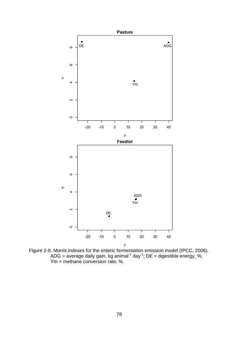
78

Figure 2-8. Morris indexes for the enteric fermentation emission model (IPCC, 2006). ADG = average daily gain, kg animal-1 day-1; DE = digestible energy, %; Ym = methane conversion rate, %.

79

Figure 2-9. Energy partitioning in animals. Adapt from: (Minson, 1990, Van Soest,

1982).

Figure 2-10. Relationship between ADG (kg animal-1 day-1) and methane production

(g CH4 ADG-1) for simulations made with Tier 2 enteric fermentation model (IPCC, 2006) for animals on pasture and feedlot.

80

CHAPTER 3 RUMINAL METHANE EMISSIONS, FORAGE AND ANIMAL PERFORMANCE

RESPONSES TO DIFFERENT STOCKING RATES ON CONTINUOUSLY STOCKED BAHIAGRASS PASTURES

Literature Review

Bahiagrass (Paspalum notatum) is an important pasture species in the US

and is cultivated in a large area in the country, from southern regions to east Texas

and central Tennessee. This species covers over 2 million hectares in the southern

USA (Newman et al., 2011) and over one million hectares in Florida (Chambliss and

Sollenberger, 1991). In north Florida, bahiagrass growing season extends from April

to November while in the southern part of the state bahiagrass grow mainly from

March to mid-December (Chambliss and Sollenberger, 1991).

Bahiagrass is adapted to a wide variety of soil types and soil pH (Chambliss

and Sollenberger, 1991; Twidwell et al., 1998) and climates (Chambliss and

Sollenberger, 1991). It is a warm-season perennial grass that reproduces by seed

(Burton, 1955) and it can achieve 225 to 560 kg of seed ha-1 when properly

managed (Chambliss and Sollenberger, 1991). It has a prostrate habit with shallow

rhizomes (Newman et al., 2011). Bahiagrass can be used for the production of hay

and grazing and is able to support heavy grazing at low soil fertility levels (Twidwell

et al., 1998), presenting high persistence and being easily established (Burton,

1955). In Florida, bahiagrass is mostly used for beef cattle (Chambliss and

Sollenberger, 1991). Sollenberger et al. (1989) found an ADG of 0.41 kg head-1 day-1

for beef steers on bahiagrass but encountered a large decrease in ADG in August

and September.

Ruminants have one forestomach separated into three compartments called

reticulum, rumen and omasum. In the rumen, the anaerobic fermentation of feed

occurs as different microbes use the feed to produce volatile fatty acids (VFA) that

81

are absorbed by ruminants. They also possess a secretory stomach called the

abomasum where protein is hydrolyzed and bacteria are digested. The fermentation

that occurs in the forestomach breaks down cellulose, which is used as a nutrient by

ruminants, and allows for access to cell contents (Leek, 2004). Methane accounts for

30 to 40 % of gases produced during enteric fermentation in ruminants (Leek, 2004),

and it can be eliminated through eructation, the lungs or the anus. Around 94- 96%

of the CH4 produced in the rumen is eliminated through eructation, whereas the

remaining CH4 is eliminated through the lungs. The CH4 produced in the animal’s

hind gut sums to 10% of total CH4 produced and is mainly excreted through the

lungs (89%), with a small part being eliminated via the anus (11%) (Murray et al.,

1976).

The microbial population inside the rumen is composed of different

microorganisms. The primary bacteria degrade cellulose or starch, while secondary

bacteria use end products from primary bacteria to obtain energy. Protozoa use

several substrates as the energy sources, including starch, polyunsaturated fatty

acids and ruminal bacteria. The function of fungi in the rumen is yet not well

understood. Microbes use mainly hydrolysis and anaerobic oxidation (removal of

hydrogen) reactions to obtain energy, creating a need for other reactions that use

this hydrogen. This need is fulfilled by methanogenic reactions (Leek, 2004),

mediated by obligate anaerobic microorganisms from the Archaea family. In the

rumen, hydrolysis of cellulose and hemicellulose releases glucose, which is then

fermented (Demeyer and Fievez, 2000). Because this reaction occurs in an

anaerobic environment, it needs electron receptors other than oxygen for

regenerating reaction co-factors like NAD+, NADP+ and FAD+ through oxidation,

which guarantees that the substrate will continue to be oxidized. However, the

82

oxidation of the co-factor is inhibited by the presence of H2 in the rumen.

Methanogenic bacteria use the hydrogen to produce CH4, thus eliminating it from the

ruminal environment and allowing for the re-oxidation of co-factors (Demeyer and

Fievez, 2000). Production of H2 also occurs from the oxidation of pyruvate into

acetate by the S organisms (Bryant et al., 1967) and is used by methanogenic

bacteria to reduce CO2 and produce CH4. Experiments suggest that the presence of

methanogenic bacteria improves the metabolism of pyruvate (Reddy et al., 1972).

The CO2 used in this reaction comes either from the decarboxylation reactions that

occur during fermentation or from the neutralization of the H+ by HCO3- (Leek, 2004).

The reactions that produce or use hydrogen inside the rumen are as follows (Ørskov

et al., 1968; Moss et al., 2000):

Glucose 2 pyruvate + 4H

Pyruvate + H2O acetate + CO2 + 2H

Pyruvate + 4H propionate + H2O

2 acetate + 4H butyrate + 2H2O

CO2 + 8H CH4 + 2H2O

One mole of glucose can form two moles of acetic acid, two moles of

propionic acid or 1 mole of butyric acid, as seen above. The production of CH4 in the

rumen requires the presence of hydrogen to reduce CO2. The formation of propionic

acid utilizes hydrogen hence reducing CH4 production, whilst increasing acetate

formation in the rumen leads to an increase in available hydrogen for CH4 production

(Ørskov et al., 1968). The acetate to propionate ratio is a good indicator of

methanogenic potential in diets. Forage fed cattle can have an acetate:propionate

ratio up to 4:1, while animals on grain diets have an acetate:propionate ratio of 1:1

(Russel, 2002).

83

There are different techniques used to measure CH4 emissions from

ruminants, each having advantages and disadvantages and being more adequate for

specific experimental conditions (Storm et al., 2012). These are the SF6 tracer gas

technique (Johnson et al., 1994), the open- circuit chamber technique (Brown et al.,

1984), the tunnel technique (Murray et al., 1999), micrometeorological mass

difference (Harper et al., 2011) and the in vitro technique (Storm et al., 2012). A brief

description of these follows.

The sulfur hexafluoride (SF6) tracer technique is used to estimate CH4

emission rates by ruminants in production conditions, including grazing (Johnson et

al., 2007), and is useful to assess several aspects of feeding and nutrition such as

influence of chemical and physical feed composition or additives on CH4 emissions

(Storm et al., 2012). It is important to notice that this technique does not measure

CH4 produced in the hindgut that is not absorbed by the bloodstream (Johnson and

Johnson, 1995). Some of the advantages of the SF6 tracer technique summarized by

Storm et al. (2012) are that animals are allowed to move freely when carrying the

equipment, so that this technique can be used during grazing trials on which animal

performance data is also measured. Also, the results are useful to analyze variation

in CH4 emission rates within and between animals and can be related to production

aspects such as milk yield and weight gain. The technique can be used to assess

almost all feeding aspects important in animal production. Studies comparing the

SF6 tracer technique with chamber measurements (technique described below)

found no significant difference among these methods (Johnson et al., 1994, 2007). In

addition, animal acclimation for the use of the SF6 tracer technique takes some days

to a week, a short period of time when compared with the weeks necessary for the

use of calorimetry chambers (Johnson et al., 1994). However, Storm et al. (2012)

84

emphasize that this technique is not suitable to evaluate differences in the emissions

through the day and that the results are more variable than in experiments made

using chambers, hence more animals are necessary when performing animal CH4

measurements using this technique.

Chambers used in CH4 measurements can be of the open or close circuit

types (Storm et al., 2012). Open-circuit indirect calorimetry chambers are used to

analyze how modifications in nutritional state, activities or environmental temperature

affect the metabolic rate of living beings during a short period (Brown et al., 1984).

When used to measure CH4 emissions by animals, this method is useful to analyze

nutrition and feeding influence on emissions and can be used to obtain results of

emissions of CH4 throughout the day (Storm et al., 2012). With this methodology,

measurements are obtained using infra-red or paramagnetic analyzers that give

results proportional to the molecular density of the gas. These measurements are

used in a series of equations to estimate volume of gas and corrected to conditions

of temperature and pressure (STP). The rate of increase of the volume of a given

gas inside the chamber is calculated as the sum of rate of volume production and

flow of the gas inside the chamber minus the rate of volume flow outside the

chamber (Brown et al., 1984). When measuring CH4 emission rates using open-

circuit respiration calorimetry chambers, the concentration of CH4 is analyzed in the

air that comes in and out the chamber constantly during the experimental period

using infrared analyzers (Johnson et al., 1994). Among the difficulties presented by

the use of the chamber methods in CH4 emission evaluations are the training

necessary for animal’s acclimation to the chamber, a process that can take several

weeks and the chamber’s high cost. Also, restrictions to the animal’s natural

85

behaviour may make this method unsuitable for extrapolation to real production

situations (Johnson et al., 1994).

Similar to the chambers, the tunnel methodology analyzes the air flowing in

and out of a tunnel for CH4 concentration, air speed and temperature (Murray et al.,

1999). This system was designed to provide animals with an environment as similar

to natural conditions as possible (Lockyer and Jarvis, 1995). When using this

methodology CH4 emissions by animals seem to be lower than other estimates

(Lockyer and Jarvis, 1995; Murray et al., 1999).

Another technique useful to measure CH4 emissions from animals in either

grazing or feedlot conditions is the micrometeorological mass difference approach,

where the flux of gases of interest in the free atmosphere is measured while

maintaining animals in their natural environment (Harper et al., 2011). This technique

requires less animal handling, therefore the animals maintain their natural behavior

(Harper et al., 2011). In this technique CH4 concentration in the air is analyzed using

infrared gas analysis or gas chromatography at different heights around the area

frequented by animals under study. This information combined with data on wind

speed and direction provides values of CH4 flux (Harper et al., 1999). The

micrometeorological technique is useful for analyzing production systems, however

little is known about its reliability (Storm et al., 2012).

The in vitro technique is a rapid and low-cost approach when assessing how

additives influence CH4 emissions because it is fast and relatively inexpensive. In

this procedure, feeds are incubated in a container with a medium combining rumen

fluid, a buffer solution and minerals. Data on CH4 production are obtained from the

analysis of gas composition and production 24 hours after incubation, usually.

Degradation of feed must be analyzed to guarantee that CH4 production is not

86

decreased because of decreased feed degradation (Storm et al., 2012). Bhatta et al.

(2008) analyzed CH4 emissions by goats fed at 1.1 times maintenance with nineteen

different diets using open circuit respiration chambers and in vitro methodology. The

authors found that emissions from both methodologies were quite similar particularly

for diets with high proportions of structural carbohydrates. Feeding Holstein cows at

a maintenance level with five different diets, Bhatta et al. (2006) found correlation

values between the SF6 tracer and in vitro gas production technique of 0.75 and 0.94

for incubations of 24 and 48 hours, respectively.

Many factors affect CH4 production by cattle, including manipulation of the

diet fed to animals (processing, addition of lipid to diet, type of carbohydrate offered

in feed), modification of ruminal microflora and management of animal intake

(Johnson and Johnson, 1995), on which animal performance is greatly dependent

(Poppi et al., 1997). Martin et al. (2009) affirm aspects that should be considered in

mitigation strategies are the decreased in H2 production in the rumen while

maintaining feed digestion, modifying the end products from the H2 utilization

reactions and inhibiting methanogenic bacteria. Animal breeding has also been

suggested as an alternative to reduce CH4 emissions from ruminants not only

directly, but also by improving animal efficiency (conversion of feed into products like

meat and milk), productivity (reducing the number of animals needed for production)

and reduction of losses such as empty reproductive cycles (Wall et al., 2009).

Some work has focused on feed manipulation for decreasing CH4 production

in ruminants by the use of additives. Bhatta et al. (2008) found several by-products

that reduced CH4 emissions in goats, such as pumpkin and brewer’s grains and

sweet potato vine silage. Tannin has also been studied and resulted in lesser CH4

emissions in goats (Puchala et al., 2005) and sheep (Carulla et al., 2005), but tannin

87

had no effect on cattle in reducing emissions, where it had bound protein

(Beauchemin et al., 2007). Other additives like canola oil reduce CH4 production in

ruminants but negatively affect animal intake and fiber digestibility, thus possibly

affecting animal performance (Beauchemin and Mcginn, 2006). Moe and Tyrrell

(1979) suggested that the nature of carbohydrates in ruminant diets can affect

production of CH4 particularly at intakes higher than 1.5 times maintenance.

Increases in digestible cellulose in diets can drive fermentation from the formation of

propionate to methanogenesis. According to Russel (2002), access to cell contents

can be decreased by the presence of lignin in the plant’s fiber, which microbial

cellulases cannot break. The presence of lignin can also hinder rumination and

therefore decrease feed particle reduction. Production of CH4 was found to be

positively related to apparent cellulose digestibility (Pinares-Patio et al., 2003) and to

type of carbohydrates in high intake diets (Moe and Tyrrell, 1979).

Animal CH4 measurements have also been performed in grazing trials, where

management practices and pasture species effect on CH4 emissions were

investigated. McCaughey et al. (1999) found lower emissions for animals grazing

alfalfa (Medicago sativa L.)/grass (meadow bromegrass, Bromus biebersteinii Roem

and Schult) than for animals grazing on grass only (meadow bromegrass, Bromus

biebersteinii Roem and Schult). Kurihara et al. (1999) found that emissions were

higher for heifers eating mature angletongrass (Dicanthium aristatum) with lower N

content than for those grazing on rhodes grass (Chloris gayana) with medium

digestibility and N content. Some studies have analyzed grazing management’s

effect on CH4 emissions. The use of BMPs (intensive grazing, rotational stocking

rate, overseeding ryegrass and fertilization) was found to result in lower CH4

production when animals were grazing on bahiagrass and bermudagrass (Kurihara

88

et al., 1999). McCaughey et al. (1997) found a significant difference in CH4

emissions when studying animals on continuously stocked alfalfa-grass (Roem and

Schult, Bromus biebersteinii; Russian wildrye, Psathyrostachys juncea (Fisch.)

Nevski) at two stocking rates. In that study, the treatment with higher stocking rate

had lower CH4 day-1 when compared to lower stocking rates. However, management

strategies and their effect on CH4 emission still need further investigation. Despite

the importance of the beef industry in Florida, no measures of CH4 emissions for

animals on pasture exist in this state.

The objective of this study was to measure CH4 emissions, animal

performance and forage characteristics of animals continuously stocked on

bahiagrass pastures at three stocking rates.


Experimental Site

This experiment was carried out during the summer of 2012 at the North

Florida Research and Education Center (NFREC) in Marianna (Jackson County),

Florida (Latitude: 30° 42’ N Longitude: 85° 13’ W). The area used for the experiment

had bahiagrass established in 2010 and was previously used for evaluations of

herbage production under different N applications. In April 2012 the area was evenly

fertilized with 57 kg ha-1 of N from ammonium nitrate (NH4NO3). The experimental

area was located in two experimental sites Figure 3-1. Soil types at the experimental

sites are described on Table 3-1 The climate in the region where the experiment was

conducted is classified as warm temperate, fully humid with hot summers (Cfa)

according to the Köppen-Geiger classification (Kottek et al., 2006).

89

Treatments and Design

The treatments in this experiment were defined as stocking rates (SR) of 1.2,

2.4 and 3.6 AU ha-1 where one animal unit (AU) is 470 kg. The bahiagrass pastures

were continuously stocked under the described fixed stocking rates during the

grazing season of 2012, meaning that a fixed number of animals was kept in each

experimental unit during the entire experimental period. The animal’s initial

liveweight was 347 ± 29 kg and it was estimated that animal average daily weight

gain would be approximately 0.46 kg/day (Stewart, 2003) during a 84-day period,

which would result in an average weight of 366 kg in the experimental period. Each

experimental unit was 1.3 ha in area. To achieve the target SRs of 1.2, 2.4 and 3.6

AU ha-1 the number of animals used was 2, 4 and 6 animals pasture-1. These

treatments were chosen with the objective of achieving differences in animal intake

and were determined on the estimated carrying capacity of the pastures according to

the N fertilization rates applied in the experimental area (57 kg N ha-1), based on

Twidwell et al. (1998) and Stewart (2003).

The experiment was initiated on 25 June and ended on 18 September 2012.

This time included three equal periods of 28 days each (Period 1: 25 June to 22 July;

Period 2: 23 July to 19 August; Period 3: 20 August to 18 September). The

experimental units were arranged in two blocks located in adjoining areas. Each

block contained 6 pastures of 1.3 ha, and so the total number of experimental units

was 12. The three treatments were replicated four times such that two replicates of a

treatment were randomly assigned to each block (randomized complete block).

Pasture and Animal Management

Herbage mass, herbage accumulation and herbage nutritive value were

measured. Herbage mass was estimated using the double sampling technique which

90

associates direct and indirect measurements of herbage mass (Santillan et al.,

1979). The indirect measurement was taken using a disk meter, where a 0.25 m2

aluminum disk was dropped always from the same height and settling height

recorded. Every 28 days, three sites representing low, medium and high herbage

mass were sampled per experimental unit. At these sites, disk meter settling height

was measured (indirect measurement) and with the help of a circular quadrat with

the same area of the disk the forage beneath the disk was clipped (direct

measurement). The pasture samples were dried at 60C until constant weight (48 to

72 hours). Calibration equations were obtained for each of the three sampling dates

with disk height as a dependent variable to herbage mass (Table 3-2). Every 14

days, disk meter settling height was measured at 30 locations per pasture, with

sampling units separated by the same number of steps in each experimental unit.

Average disk meter settling height was inputted in the calibration equation to

estimate herbage mass.

To estimate herbage accumulation rate (HAR), three 1 m2 exclusion cages

were installed per pasture at the beginning of the experimental period at sites where

the disk meter measurements were ±1 cm from average disk meter measures for

that pasture. Every 14 days, disk height was measured inside the cage. The cages

were then relocated to sites in the pasture that had the same disk settling height (±1

cm) of the rest of the pasture. Herbage mass was estimated using the calibration

equation for the period. Herbage accumulation rate was calculated as follows:

HAR (kg ha-1 day-1) = [Cage HM (kg ha-1) day 2 -Cage HM (kg ha-1) day 1] / days

Every 14 days, one sample composed of 20- 25 hand plucked subsamples

per pasture was collected and used to measure nutritive value (crude protein, CP;

neural detergent fiber, NDF; acid detergent fiber, ADF). After collection, the samples

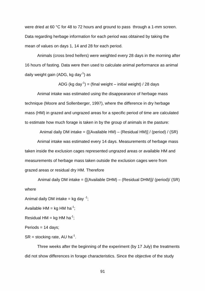
91

were dried at 60 °C for 48 to 72 hours and ground to pass through a 1-mm screen.

Data regarding herbage information for each period was obtained by taking the

mean of values on days 1, 14 and 28 for each period.

Animals (cross bred heifers) were weighted every 28 days in the morning after

16 hours of fasting. Data were then used to calculate animal performance as animal

daily weight gain (ADG, kg day-1) as

ADG (kg day-1) = (final weight – initial weight) / 28 days

Animal intake was estimated using the disappearance of herbage mass

technique (Moore and Sollenberger, 1997), where the difference in dry herbage

mass (HM) in grazed and ungrazed areas for a specific period of time are calculated

to estimate how much forage is taken in by the group of animals in the pasture:

Animal daily DM intake = {[(Available HM) – (Residual HM)] / (period) / (SR)

Animal intake was estimated every 14 days. Measurements of herbage mass

taken inside the exclusion cages represented ungrazed areas or available HM and

measurements of herbage mass taken outside the exclusion cages were from

grazed areas or residual dry HM. Therefore

Animal daily DM intake = {[(Available DHM) – (Residual DHM)]/ (period)/ (SR)

where

Animal daily DM intake = kg day -1;

Available HM = kg HM ha-1;

Residual HM = kg HM ha-1;

Periods = 14 days;

SR = stocking rate, AU ha-1.

Three weeks after the beginning of the experiment (by 17 July) the treatments

did not show differences in forage characteristics. Since the objective of the study

92

was to use SR to create differences in forage characteristics and study their effects

on CH4 production by animals and animals performance, 1, 2 and 3 AU ha-1 were

added to the experiment in the treatments 1.2, 2.4 and 3.6 ha-1, respectively. These

animals remained in the experimental units for three weeks. Animal weight data from

these animals were not considered in the analysis of average daily gain.

Ruminal Methane Emissions Measurements

Two CH4 collection periods occurred starting 8 July and 10 September 2012

using the technique described in Johnson et al. (2007). One collection period

consisted of five consecutive days of measurements and results of CH4 production

per day were averaged to obtain one value per animal per period. Methane emission

rate was also averaged between the animals within each experimental unit. Twenty

four animals previously used in another experiment for CH4 measurements were

used in this study so that two animals per experimental unit were used for the CH4

measurements. In these animals, one permeation tube with a known SF6 released

rate was placed in the animal’s rumen. These permeation tubes were purchased

from Washington State University, where they were calibrated in hot water bath at 39

°C to achieve a constant release rate of between 1 and 2 mg day-1. Average SF6

release rate was of 1.7597 mg day-1. The collection of air around the animal’s mouth

and nostrils was made through a capillary tube place on the top of the animal’s nose.

This capillary was attached to a halter and is connected through a valve to a PVC

canister evacuated to -27 mm Hg (Figure 3-2). Samples were collected to a pressure

of -13.5 mm Hg. Data from canisters returning with pressures above -10 mm Hg or

below -20 mm Hg were not considered. Any animals which did not have at least

three days of collection were not considered in the analysis. Collection time to

achieve the final pressure was 24 h and was regulated by the length of the capillary

93

tube. In the first day of each collection period a halter and an evacuated yoke were

placed on the animals. After 24 h, the yoke collecting the sample was retrieved and a

new, evacuated canister was placed on the animals, connected to the yoke, and the

valve was opened. This procedure was repeated for five consecutive days. On every

collection day, two canisters were used to collect air and one placed at the center of

each experimental area (A and B Figure 3-1) that served to analyze background

(ambient) concentrations of CH4 and SF6.

The canisters containing the sample were taken to the lab for analysis lab and

allowed to cool until they reached environmental temperature. They were then

pressurized with N until 3 psi and CH4 and SF6 concentrations were measured twice

from each canister using gas chromatography (Agilent 7820A GC, Agilent

Technologies, Palo Alto, CA) equipped with a flame ionization detector and a

capillary column (Plot Fused Silica 25 m × 0.32 mm, coating Molsieve 5A, Varian

CP7536).

Every collection day, pure standards were used to obtain a calibration curve

for CH4 and SF6. After this, the canisters were rinsed ten times with pressured air. To

obtain the values of g CH4 day-1, the following equation was used:

QCH4 = QSF6 x [(CH4 - CH4 A) / (SF6 - SF6 A)]

where

QCH4 is CH4 emissions rate, g day-1;

QSF6 is the SF6 release rate

CH4 and SF6 are the concentration in the yoke

CH4 A e SF6 A are the concentrations in the ambient.

The correction for background SF6 concentrations were followed as

suggested by (Lassey, 2013). QCH4 outliers (mean ± 2 SD) were eliminated.

94

Statistical Analysis

Statistical analysis was performed using SAS. Response variables were

herbage mass (HM), herbage accumulation rate (HAR), CP, ADF, NDF, average

daily gain (ADG), body weight (BW), dry matter intake (DMI) (kg animal-1 day-1, kg kg

BW-1 day-1) and CH4 (g CH4 day-1, g CH4 kg BW-1 and g CH4 kg DMI-1). Data were

analyzed using repeated measures analysis of variance using PROC MIX model of

SAS. Periods were considered repeated measures and pasture (experimental unit)

was considered to be the experimental unit. SR, period and SR x period were fixed

effects. Block and interactions with block were considered random.

Results

Results of the effect of treatment (different SR on continuously stocked

bahiagrass), period and treatment x period interaction are summarized in Table 3-3.

Forage nutritive value was affected by period but no treatment or treatment x period

effect were observed on animal or plat related response variables. There was no

effect of treatment or period on animal related variables, including the measures of

CH4 (g CH4 day-1, g CH4 kg BW-1 and g CH4 kg DMI-1).

Discussion

The values of HM (presented on Figure 3-3) found in this study are similar to

those previously reported in the literature. Chambliss and Sollenberger (1991)

reported values varying between 2600 and 6330 for the summer in Florida. There

was an increase in HM through the grazing season with higher values observed in

August. This pattern was different than that observed by others (Johnson et al.,

2001b; Stewart, 2003), where HM peaked by the end of June and July. The

difference might be related to the rainfall pattern observed during the experimental

period. In July, rainfall was 139 mm and reached 367 mm in August. There was no

95

effect of treatment or period in HAR. Values of HAR ranged from 57 to 67 kg HM ha-1

day-1. These values are in the range of previously reported studies. Inyang et al.

(2010) found values of 106, 128 and 118 kg HM ha-1 day-1 on continuously stocked

bahiagrass. The lower HAR observed might have been caused by the lower rainfall

observed in the months of June and July in the present study. Stewart Jr. (2003)

evaluated bahiagrass under low, moderate and high management (1.2, 2.4 and 3.6

AU ha-1 with applications of 40, 120 and 360 kg N ha-1, respectively). The author

found significantly higher HAR at moderate and high management treatment

achieving values of as high as 37 kg ha-1 day-1. At low management levels, average

HAR was 19 kg ha-1 day-1.

A tendency to treatment effect and an effect of period were observed for

values of CP, but no treatment x period interactions were observed (Figure 3-10).

Period also had a positive effect on CP with values 8.8, 9.2 and 9.5% Periods 1, 2

and 3, respectively. Values of CP between 9.9 and 12% were reported for

rotationally stocked bahiagrass, with values increasing after September

(Sollenberger et al., 1989). On continuously stocked bahiagrass, Stewart (2003)

found values of CP varying between 9.2 and 14.3% with significantly higher values of

CP with more intense management (higher SR and N fertilizer application). Cuomo

et al. (1996) evaluated the nutritive value of Argentine and Pensacola bahiagrass

under different cutting frequencies (20, 30 and 40 days) in two years. Values

reported by Cuomo et al. (1996) were of 14% and 10% for CP in early (late May to

end of June) and late (mid-August to mid-September).

For NDF, no treatment effect was observed. There was a period effect on

NDF which increased through the grazing season (Figure 3-9). Other authors also

found an increase in NDF concentration of bahiagrass through grazing seasons.

96

NDF increased through the grazing season from the range of 73 to 86% to the range

of 79 to 82% (Grise et al., 2006). These values are higher than those observed in the

present study. However, the values presented by Grise et al. (2006) refer to whole-

plant samples and do not represent the grazed proportion of the pasture. In this

case, nutritive value might be underestimated (Sollenberger and Cherney, 1995).

There was no effect of treatment on ADF, but a period effect was observed

with increasing ADF concentration as the season progressed. Other studies have

also found differences in ADF through grazing season in bahiagrass. Cuomo et al.

(1996) found lower values of ADF for bahiagrass in early summer (May to June). .

No effect of SR or period on ADG was observed. The ADG was lower than

what has been observed for continuously stocked bahiagrass with values varying

between 0.22 to -0.18. Inyang et al. (2010) observed a linear decrease in ADG with

increasing of SR (4, 8 and 12 heifers ha-1). Low ADG of animals grazing bahiagrass

and bermudagrass was also observed during summer and fall by DeRamus et al.

(2003). Sollenberger et al. (1989) found an ADG of 0.41 kg head-1 day-1 when

crossbred yearling steers grazed on bahiagrass from April through November but

encountered a large decrease in ADG in August and September. Stewart (2003)

evaluated bahiagrass under low, moderate and high management (1.2, 2.4 and 3.6

AU ha-1 with applications of 40, 120 and 360 kg N ha-1, respectively) and found that

ADG decreased with higher management levels. However, gain per hectare in that

study was smaller at low management levels.

There was no effect of SR or period on DMI expressed as kg animal-1 day-1 or

kg (kg BW)-1 day-1. Values of DMI (kg animal-1 day-1) found were higher than

expected achieving values as high as 22 kg animal-1 day-1. Undi et al. (2008)

compared the use of herbage mass disappearance technique with the use of

97

alkanes and two prediction equations for measuring intake. The author found that

estimation of DMI using the herbage disappearance technique was greater than any

of the other techniques, achieving values of 14.3 to 18.9 kg DMI day-1. The authors

suggest that the trampling of the pasture might be the cause of this overestimation of

DMI. It has been found that DMI is linearly related to CH4 emissions (g animal-1 day-

1) for cattle grazing tropical forages (Kurihara et al., 1999). However, no linear or

quadratic relationship was found between CH4 (g day-1) and DMI (kg animal-1 day-1).

There was no effect of treatment or period on CH4 emissions expressed as g

CH4 day-1, g CH4 kg BW-1 and g CH4 kg DMI-1 (Figure 3-11, Figure 3-12 and Figure 3-

13). The coefficient of variation (CV, %) within animals was 79 and 86% in the first

and second periods of CH4 collection. Although these CVs are higher than those

reported in the literature, large variation in CH4 production between animals has

been reported in other studies using the SF6 technique. In sheep fed chaffed lucerne

hay diets, between individual variation was responsible for 70% of variation in CH4

production (Pinares-Patio et al., 2003). In cattle fed different forages with different

qualities, CV (%) values for CH4 emission above 26% were observed in both day- to-

day and animal- to- animal measurements (Boadi et al., 2004). However, the authors

emphasized that these high values might be related to the diverse feeding conditions

and small number of animals. This large CV is one of the reasons why no statistical

differences between treatments or periods were detected.

The values of CH4 emissions varied between 140 to 879 g CH4 day-1. The

values found in the present study were higher than what was previously reported for

animal grazing bahiagrass. For animals grazing bahiagrass under normal or BMP

management (overseeding of ryegrass and fertilization), lower values of CH4

emissions were found under BMP management (DeRamus et al., 2003). Values of

98

daily CH4 emissions for cows and heifers of 120 to 249 g day-1 and 86 to 166 g day-1

were reported (DeRamus et al., 2003). High values of CH4 emissions were found for

dairy cattle and lactating beef cattle. For dairy cattle grazing perennial ryegrass and

white clover, Ulyatt et al. (2002) found varying values of CH4 emissions through the

season between 137 and 431 g day-1. The seasonal variation was closely related to

milk production and estimated animal intake. For lactating beef cattle grazing alfalfa-

grass or bromegrass pastures, CH4 emissions of 267- 293 g day-1 were reported

(McCaughey et al., 1999). McCaughey et al. (1997) found a difference in CH4

emissions when studying animals on continuously stocked alfalfa (Medicago sativa)-

grass (Roem and Schult, Bromus biebersteinii; Russian wildrye, Psathyrostachys

juncea (Fisch.) Nevski) with two stocking rates. In that study, the treatment with

higher stocking rate had lower CH4 day-1 when compared to lower stocking rates.

Kurihara et al. (1999) suggested that the CH4 conversion rate of tropical forages is

higher than those from temperate species, i. e., more energy is used in the

production of CH4 when animals are fed tropical forages.

Although some authors conclude that DM intake can be used to predict CH4

production by adult cattle on maintenance (Moe and Tyrrell, 1979), more studies are

necessary to confirm if the linear relationship between DM intake and CH4 emissions

(g animal-1 day-1) for cattle grazing tropical forages may be used for prediction

(Kurihara et al., 1999). In that study, authors found that CH4 emission rate is reduced

at high feed levels and energy intake in comparison to animals kept on maintenance

level, probably due to greater rate of passage of feed in the animals’ digestible tract

and consequent reduction in feed fermentation time. This difference in CH4 energy

according to animal’s feeding level was also observed by Moe and Tyrrell (1979) in

dairy cattle, and the authors concluded that type of carbohydrate influences CH4 in

99

dairy cattle at higher intakes but do not significantly affect CH4 prediction at lower

intakes. Another study conducted by Boadi and Wittenberg (2002) where animals

were fed hay varying in IVOMD concluded that DM intake could be used to predict

CH4 emissions from animals fed ad libitum, and DMI represented 64% of variation in

CH4 emissions. Although several studies show a relationship between CH4

emissions and intake, there was no correlation of these two variables in this study.

Information on initial weight and ADG of each treatment on Periods 1 and 3

were used in the IPCC (Tier 2) method to estimate emissions in g CH4 day-1. Results

are presented in Figure 3-14, where the default value suggested by IPCC (2006) for

the Tier 1 method is also presented. It is evident that the values from the field

measures were much more variable than that obtained using the Tier 2 approach.

Results obtained by the Tier 2 approach do not differ greatly due to treatment. This is

probably related to the very similar ADG values encountered in the field experiment

and used in the simulation, since it was found that the model is very sensitive to the

ADG variable. The Tier 1 and Tier 2 approaches seem to underestimate CH4

emissions in this study, however a more detailed study on prediction capacity is

necessary.

Conclusions

The objective of this study was to measure CH4 emissions, animal

performance and forage characteristics of animals grazing continuously stocked

bahiagrass under three different stocking rates. The SR applied affected HM and

chemical value of bahiagrass, however it did not affect animal response variables.

CH4 emissions were also not affected by SR. On average, animals grazing

bahiagrass emitted 393 g CH4 day-1 and a high variation was found on emissions.

This is the first CH4 measurements for grazing animals in Florida. The IPCC Tier 2

100

and Tier 1 approaches seem to underestimate emissions of CH4 by cattle. Due to the

great importance of agriculture in Florida’s economy, it is important to obtain more

information about emissions from different agriculture-related sources. This

information may help not only to improve model use but also give a more clear

understanding of management approaches that can be used to reduce or avoid GHG

emissions.

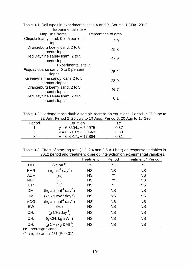
101

Table 3-1. Soil types in experimental sites A and B. Source: USDA, 2013.

Experimental site A Map Unit Name Percentage of area

Chipola loamy sand, 0 to 5 percent slopes

2.9

Orangeburg loamy sand, 2 to 5 percent slopes

49.3

Red Bay fine sandy loam, 2 to 5 percent slopes

47.9

Experimental site B Fuquay coarse sand, 0 to 5 percent

slopes 25.2

Greenville fine sandy loam, 2 to 5 percent slopes

28.0

Orangeburg loamy sand, 2 to 5 percent slopes

46.7

Red Bay fine sandy loam, 2 to 5 percent slopes

0.1

Table 3-2. Herbage mass double sample regression equations. Period 1: 25 June to 22 July; Period 2: 23 July to 19 Aug.; Period 3: 20 Aug to 18 Sep.

Period Equation R2

1 y = 6.3604x + 5.2975 0.87 2 y = 6.6018x – 0.9663 0.89 3 y = 6.8917x + 17.804 0.81

Table 3-3. Effect of stocking rate (1.2, 2.4 and 3.6 AU ha-1) on response variables in 2012 period and treatment x period interaction on experimental variables.

Treatment Period Treatment * Period

HM (kg ha-1) ** ** **

HAR (kg ha-1 day-1) NS NS NS

ADF (%) NS ** NS

NDF (%) NS ** NS

CP (%) NS ** NS

DMI (kg animal-1 day-1) NS NS NS

DMI (kg kg BW-1 day-1) NS NS NS

ADG (kg animal-1 day-1) NS NS NS

BW (kg) NS NS NS

CH4 (g CH4 day-1) NS NS NS

CH4 (g CH4 kg BW-1) NS NS NS

CH4 (g CH4 kg DMI-1) NS NS NS

NS: non-significant ** : significant at 1% (P<0.01)

102

Table 3-4. Forage herbage mass (HM) (kg ha-1) and herbage accumulation rate

(HAR) (kg ha-1 day-1) response to three stocking rates (1.2, 2.4 and 3.6 AU ha-1) in 2012. Period 1: June 25 to July 22; Period 2: July 23 to Aug. 19; Period 3: Aug.20 to Sep. 18.

Period 1 Period 2 Period 3

Stocking rate (AU ha-1)

HM (kg ha-1) SE

1.2 3235 3956 4787 198.4

2.4 3239 3661 4063 198.4

3.6 2967 2735 2983 198.4

HAR (kg ha-1day-1)

1.2 67 57 57 8.5

2.4 65 61 59 8.5

3.6 62 57 67 8.5

Table 3-5. Forage chemical composition response given by CP (%), NDF (%) and ADF (%) to three stocking rates (1.2, 2.4 and 3.6 AU ha-1) in 2012. Period 1: June 25 to July 22; Period 2: July 23 to Aug. 19; Period 3: Aug.20 to Sep. 18.


Stocking rate (AU ha-1) CP (%) SE

1.2 8.6 8.6 8.7 1.5

2.4 8.5 9.0 9.2 1.5

3.6 9.4 10.0 10.8 1.5

NDF (%)

1.2 63.2 64.8 65.4 0.6

2.4 63.2 65.6 65.4 0.6

3.6 64.5 64.2 63.6 0.6

ADF (%)

1.2 35.1 36.1 37.1 1.0

2.4 35.6 36.9 36.9 1.0

3.6 35.7 36.5 36.4 1.0

103

Table 3-6. Average daily gain (ADG, kg animal-1day-1), BW (kg animal-1), DMI (kg animal-1day-1) and DMI (kg BWl-1 day-1) response to three stocking rates (1.2, 2.4, 3.6 AU ha-1) in 2012. Period 1: June 25 to July 22; Period 2: July 23 to Aug. 19; Period 3: Aug.20 to Sep. 18.



ADG (kg animal-1day-1) SE

1.2 0.03 0.12 -0.18 0.2

2.4 0.22 -0.03 -0.03 0.2

3.6 0.12 -0.02 0.01 0.2

BW (kg animal-1)

1.2 344.9 347.1 349.2 4.7

2.4 348.4 351.0 351.1 4.7

3.6 353.3 355.8 351.9 4.7

DMI (kg animal-1day-1)

1.2 20 21 22 3.2

2.4 18 16 17 3.2

3.6 15 14 15 3.2

DMI (kg kg BWl-1day-1)

1.2 5.9 6.0 6.5 0.9

2.4 5.2 4.6 4.9 0.9

3.6 4.1 4.0 4.2 0.9

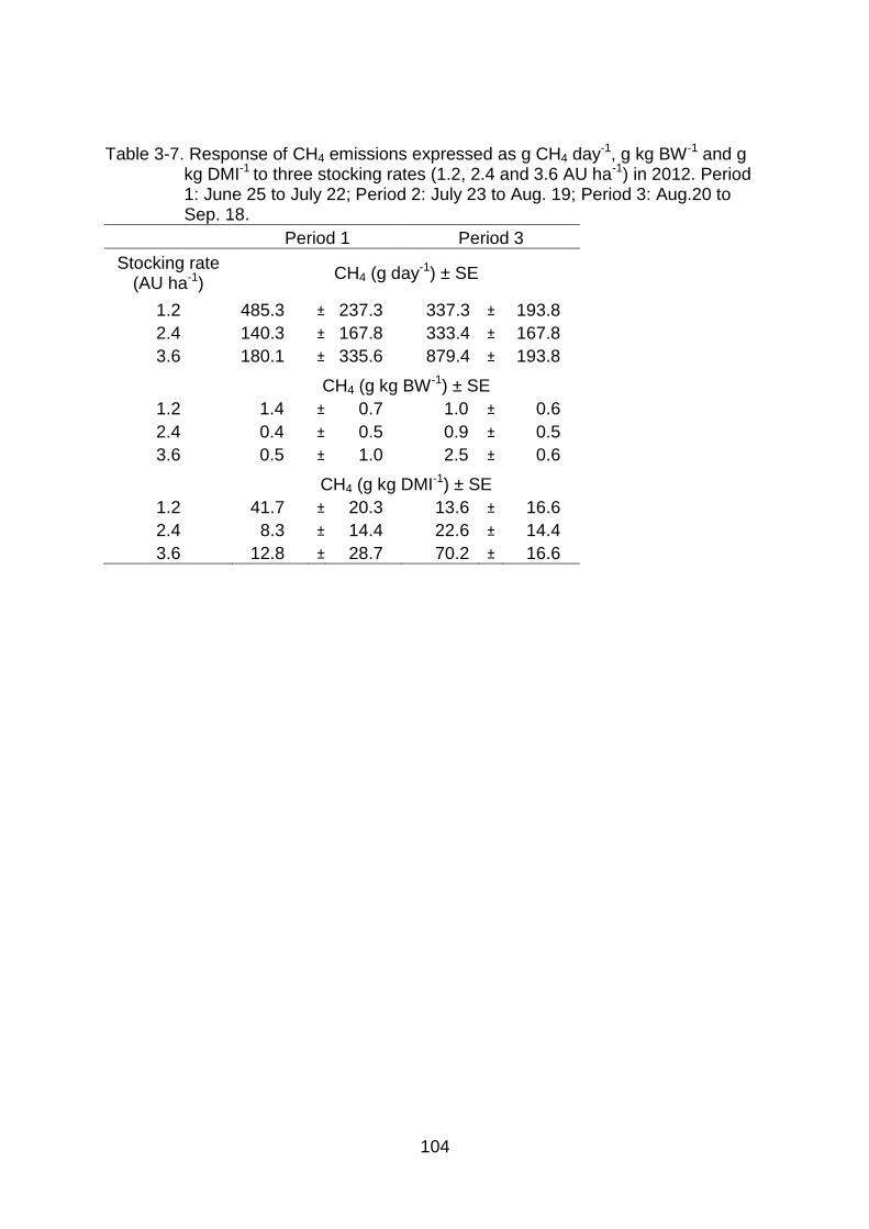
104

Table 3-7. Response of CH4 emissions expressed as g CH4 day-1, g kg BW-1 and g kg DMI-1 to three stocking rates (1.2, 2.4 and 3.6 AU ha-1) in 2012. Period 1: June 25 to July 22; Period 2: July 23 to Aug. 19; Period 3: Aug.20 to Sep. 18.

Period 1 Period 3


CH4 (g day-1) ± SE

1.2 485.3 ± 237.3 337.3 ± 193.8

2.4 140.3 ± 167.8 333.4 ± 167.8

3.6 180.1 ± 335.6 879.4 ± 193.8

CH4 (g kg BW-1) ± SE

1.2 1.4 ± 0.7 1.0 ± 0.6

2.4 0.4 ± 0.5 0.9 ± 0.5

3.6 0.5 ± 1.0 2.5 ± 0.6

CH4 (g kg DMI-1) ± SE

1.2 41.7 ± 20.3 13.6 ± 16.6

2.4 8.3 ± 14.4 22.6 ± 14.4

3.6 12.8 ± 28.7 70.2 ± 16.6

105

Figure 3-1. Map of experimental sites A and B located at the North Florida Research and Education Center (NFREC), Marianna, Florida.

Figure 3-2. Animal with CH4 collection device. A: capillary tube placed on halter; B:

collecting canister. Picture by Marta Moura Kohmann, 2012.

A

B

A

B

A

B

106

Figure 3-3. Herbage mass (kg ha-1) response to three stocking rates (1.2, 2.4 and 3.6 AU ha-1) in 2012. Period 1: June 25 to July 22; Period 2: July 23 to Aug. 19; Period 3: Aug.20 to Sep. 18.

Figure 3-4. Herbage accumulation rate (HAR) (kg ha-1 day-1) i response to three stocking rates (1.2, 2.4 and 3.6 AU ha-1) in 2012. Period 1: June 25 to July 22; Period 2: July 23 to Aug. 19; Period 3: Aug. 20 to Sep. 18.

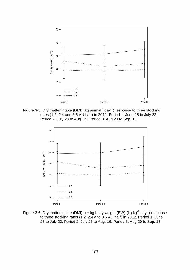
107

Figure 3-5. Dry matter intake (DMI) (kg animal-1 day-1) response to three stocking rates (1.2, 2.4 and 3.6 AU ha-1) in 2012. Period 1: June 25 to July 22; Period 2: July 23 to Aug. 19; Period 3: Aug.20 to Sep. 18.

Figure 3-6. Dry matter intake (DMI) per kg body weight (BW) (kg kg-1 day-1) response to three stocking rates (1.2, 2.4 and 3.6 AU ha-1) in 2012. Period 1: June 25 to July 22; Period 2: July 23 to Aug. 19; Period 3: Aug.20 to Sep. 18.

108

Figure 3-7. Average daily gain (ADG) (kg animal-1 day-1) response to three stocking rates (1.2, 2.4 and 3.6 AU ha-1) in 2012. Period 1: June 25 to July 22; Period 2: July 23 to Aug. 19; Period 3: Aug.20 to Sep. 18.

Figure 3-8. Acid detergent fiber (ADF) (%) response to three stocking rates (1.2, 2.4 and 3.6 AU ha-1) in 2012. Period 1: June 25 to July 22; Period 2: July 23 to Aug. 19; Period 3: Aug.20 to Sep. 18.

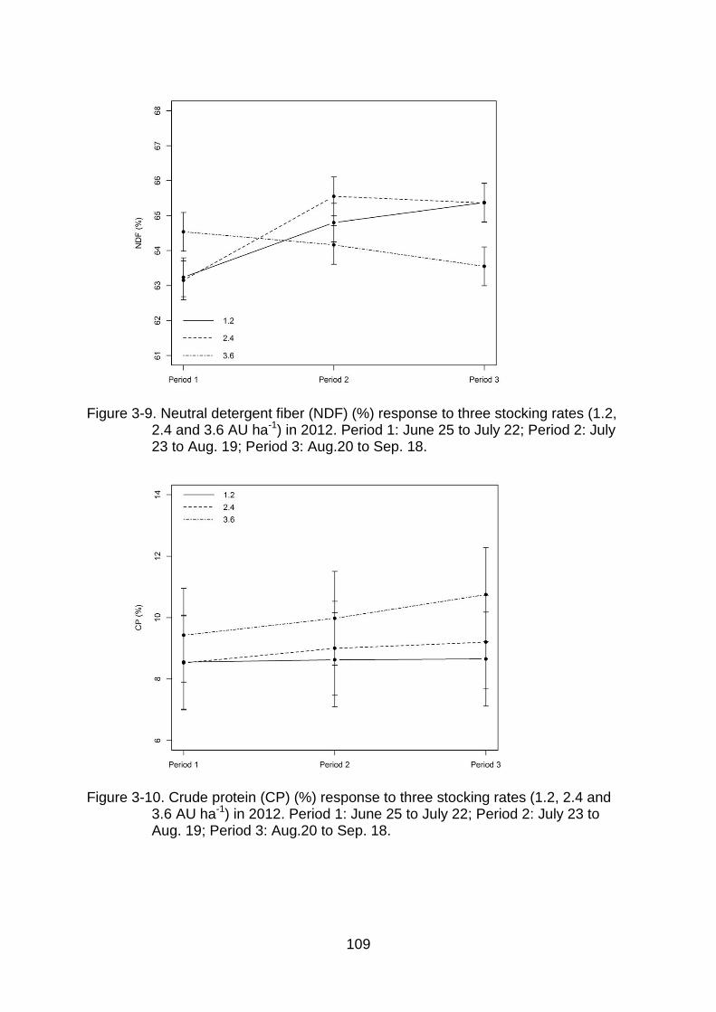
109

Figure 3-9. Neutral detergent fiber (NDF) (%) response to three stocking rates (1.2, 2.4 and 3.6 AU ha-1) in 2012. Period 1: June 25 to July 22; Period 2: July 23 to Aug. 19; Period 3: Aug.20 to Sep. 18.

Figure 3-10. Crude protein (CP) (%) response to three stocking rates (1.2, 2.4 and 3.6 AU ha-1) in 2012. Period 1: June 25 to July 22; Period 2: July 23 to Aug. 19; Period 3: Aug.20 to Sep. 18.

110

Figure 3-11. Methane production (g CH4 animal-1 day-1) response to three stocking rates (1.2, 2.4 and 3.6 AU ha-1) in 2012. Period 1: June 25 to July 22; Period 2: July 23 to Aug. 19; Period 3: Aug.20 to Sep. 18.

Figure 3-12. Methane production (g CH4 kg BW-1) response to three stocking rates (1.2, 2.4 and 3.6 AU ha-1) in 2012. Period 1: June 25 to July 22; Period 2: July 23 to Aug. 19; Period 3: Aug.20 to Sep. 18.

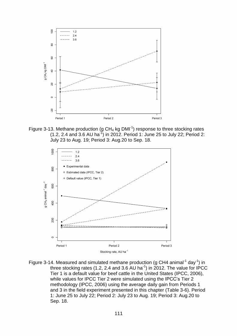
111

Figure 3-13. Methane production (g CH4 kg DMI-1) response to three stocking rates (1.2, 2.4 and 3.6 AU ha-1) in 2012. Period 1: June 25 to July 22; Period 2: July 23 to Aug. 19; Period 3: Aug.20 to Sep. 18.

Figure 3-14. Measured and simulated methane production (g CH4 animal-1 day-1) in three stocking rates (1.2, 2.4 and 3.6 AU ha-1) in 2012. The value for IPCC Tier 1 is a default value for beef cattle in the United States (IPCC, 2006), while values for IPCC Tier 2 were simulated using the IPCC’s Tier 2 methodology (IPCC, 2006) using the average daily gain from Periods 1 and 3 in the field experiment presented in this chapter (Table 3-6). Period 1: June 25 to July 22; Period 2: July 23 to Aug. 19; Period 3: Aug.20 to Sep. 18.

112

LIST OF REFERENCES

Archbolt Biological Station. 2013. Archbolt Biological Station. http://www.archbold-station.org (accessed 7 Oct 2013).

Basarab, J., V. Baron, Ó. López-Campos, J. Aalhus, K. Haugen-Kozyra, and E. Okine. 2012. Greenhouse Gas Emissions from Calf- and Yearling-Fed Beef Production Systems, With and Without the Use of Growth Promotants. Animals 2(4): 195–220.

Bauer, L.R., and D.M. Hamby. 1991. Relative Sensitivities of Existing and Novel Model Parameters in Atmospheric Tritium Dose Estimates. Bauer and Ha. Radiat. Prot. Dosimetry 37(4): 253–260.

Beauchemin, K.A., J.H. Henry, S.M. Little, T.A. McAllister, and S.M. McGinn. 2010. Life cycle assessment of greenhouse gas emissions from beef production in western Canada: A case study. Agric. Syst. 103(6): 371–379.

Beauchemin, K.A., and S.M. Mcginn. 2005. Methane emissions from feedlot cattle fed barley or corn diets. J. Anim. Sci. 83: 653–661.

Beauchemin, K.A., and S.M. Mcginn. 2006. Methane emissions from beef cattle : Effects of fumaric acid , essential oil, and canola oil. J. Anim. Sci. 84: 1489–1496.

Beauchemin, K.A., S.M. McGinn, T.F. Martinez, and T.A. McAllister. 2007. Use of condensed tannin extract from quebracho trees to reduce methane emissions from cattle. J. Anim. Sci. 85(8): 1990–1999.

Bhatta, R., O. Enishi, N. Takusari, K. Higuchi, I. Nonaka, and M. Kurihara. 2008. Diet effects on methane production by goats and a comparison between measurement methodologies. J. Agric. Sci. 146: 705– 715.

Bhatta, R., K. Tajima, N. Takusari, K. Higuchi, O. Enishi, and M. Kurihara. 2006. Comparison of sulfur hexafluoride tracer technique, rumen simulation technique and in vitro gas production techniques for methane production from ruminant feeds. Int. Congr. Ser. 1293: 58–61.

Boadi, D.A., and K.M. Wittenberg. 2002. Methane production from dairy and beef heifers fed forages differing in nutrient density using the sulphur hexafluoride (SF6) tracer gas technique. Can. J. Anim. Sci. 82: 201-206.

Boadi, D.A., K.M. Wittenberg, S.L. Scott, D. Burton, K. Buckley, J. a. Small, and K.H. Ominski. 2004. Effect of low and high forage diet on enteric and manure pack greenhouse gas emissions from a feedlot. Can. J. Anim. Sci. 84(3): 445–453.

113

Brown, D., T.J. Cole, M.J. Dauncey, R.W. Marrs, and P.R. Murgatroyd. 1984. Analysis of gaseous exchange in open-circuit indirect calorimetry. Med. Biol. Eng. Comput. 22: 333–338.

Bryant, M.P., E.A. Wolin, and Wolin, M. J., and R.S. Wolfe. 1967. Methanobacillus omelianskii, a Symbiotic Association of two Species of Bacteria. Arch. Mikrobiol. 59: 20– 31.

Burton, G.W. 1955. Breeding Pensacola Bahiagrass, Paspalum notatum; I. Method of Reproduction. Agron. J. 47(7): 311– 314.

Campolongo, F., J. Cariboni, and A. Saltelli. 2007. An effective screening design for sensitivity analysis of large models. Environ. Model. Softw. 22(10): 1509–1518.

Carulla, J.E., M. Kreuzer, A. Machmüller, and H.D. Hess. 2005. Supplementation of Acacia mearnsii tannins decreases methanogenesis and urinary nitrogen in forage-fed sheep. Aust. J. Agric. Res. 56(9): 961– 970.

Casey, J.W., and N.M. Holden. 2006. Quantification of GHG emissions from sucker-beef production in Ireland. Agric. Syst. 90: 79–98.

Chambliss, C.G., and L.E. Sollenberger. 1991. Bahiagrass: The foundation of cow-calf nutrition in Florida. Proc. 40th Florida Beef Cattle Shortcourse, Gainesville. Univ. of Florida, Gainesville, p. 74–80.

Cukier, R.I. 1973. Study of the sensitivity of coupled reaction systems to uncertainties in rate coefficients. I Theory. J. Chem. Phys. 59(8): 3873-3878.

Cukier, R.I., H.B. Levine, and K.E. Schuler. 1978. Nonlinear Sensitivity Analysis of Multiparameter Model Systems. J. Comput. Phys. 26: 1–42.

Cukier, R.I., J.H. Schaibly, and K.E. Shuler. 1975. Study of the sensitivity of coupled reaction systems to uncertainties in rate coefficients. III. Analysis of the approximations. J. Chem. Phys. 63(3): 1140-1149.

Cuomo, G.J., D.C. Blouin, D.L. Corkern, J.E. Mccoy, and R. Walz. 1996. Plant morphology and forage nutritive value of three bahiagrasses as affected by harvest frequency. Agron. J. 88: 85–89.

Demeyer, D., and V. Fievez. 2000. Ruminants et environnement : la méthanogenèse. Ann. Zootech. 49: 95–112.

DeRamus, H.A., T.C. Clement, D.D. Giampola, and P.C. Dickison. 2003. Methane emissions of beef cattle on forages: efficiency of grazing management systems. J. Environ. Qual. 32(1): 269–277.

114

Dijkstra, J., D.S.C.N. Heather, D.E. Beever, and J. France. 1992. Simulation of Nutrient Digestion, Absorption Outflow in the Rumen : Model Description. J. Nutr. (122): 2239–2256.

Environmental Protection Agency. 2005. Emission Facts: Average Carbon Dioxide Emissions Resulting from Gasoline and Diesel Fuel. U. S. Gov. Print. Office, Washington DC.

Environmental Protection Agency. 2013a. Inventory of U. S. Greenhouse Gas Emissions and Sinks : 1990- 2011. U. S. Gov. Print. Office, Washington, DC.

Environmental Protection Agency. 2013b. ANNEX 3 Methodological Descriptions for Additional Source or Sink Categories. U. S. Gov. Print. Office, Washington, DC.

Florida Department of Agriculture and Consumer Services. 2012. Florida agriculture by the numbers. http://www.nass.usda.gov/Statistics_by_State/Florida/Publications/ Agriculture_Statistical_Directory/2012/2012%20FL%20Ag%20by%20the%20Numbers(FASD).pdf (accessed 12 Sept. 2013).

Foley, P. A., P. Crosson, D.K. Lovett, T.M. Boland, F.P. O’Mara, and D. A. Kenny. 2011. Whole-farm systems modelling of greenhouse gas emissions from pastoral suckler beef cow production systems. Agric. Ecosyst. Environ. 142(3-4): 222–230.

Grise, M.M., L. Sollenberger, J.C. Dubeux Jr., S. Interrante, R.L. Stewart, and A. Pelissari. 2006. Biomass allocation and forage quality in a pensacola bahia grass pasture in north central Florida. Acta Sci. Anim. Sci. 28(4): 375– 383.

Harper, L.A., O.T. Denmead, and T.K. Flesch. 2011. Micrometeorological techniques for measurement of enteric greenhouse gas emissions. Anim. Feed Sci. Technol. 166-167: 227–239.

Harper, L.A., O.T. Denmead, J.R. Freney, and F.M. Byers. 1999. Direct measurements of methane emissions from grazing and feedlot cattle. J. Anim. Sci. 77 : 1392–1401.

Inyang, U., J.M.B. Vendramini, L.E. Sollenberger, B. Sellers, A. Adesogan, L. Paiva, and A. Lunpha. 2010. Forage Species and Stocking Rate Eff ects on Animal Performance and Herbage Responses of “ Mulato ” and Bahiagrass Pastures. Crop Sci. (20): 1079–1085.

IPCC. 2006. 2006 IPCC Guidelines for National Greenhouse Gas Inventories. In: Eggleston, H.S., L. Buendia, K. Miwa, T. Ngara, and K. Tanabe, editors. IGES, Japan.

IPCC. 2007a. Climate Change 2007: Synthesis Report. Contribution of Working Groups I, II and III to the Fourth Assessment Report of the Intergovernmental Panel on Climate Change. In: Pachauri, R. K.; A. Reisinger, editors. Geneva, Switzerland.

115

IPCC. 2007b. Climate change 2007: the Physical Science Basis. In: Solomon, S., Qin, D., Manning, M., Chen, Z., Marquis, M., Averyt, K.B., Tignor, M., Miller, H.L., editors, Contribution of Working Group I to the Fourth Assessment Report of the Intergovernmental Panel on Climate Change. Summary for Policymakers. Cambridge University Press, Cambridge, United Kingdom and New York, NY, USA.

IPCC. 2013. Organization. http://www.ipcc.ch (accessed 20 Oct. 2013).

Johnson, K., M. Huyler, H. Westberg, B. Lamb, and P. Zlmmerman. 1994. Measurement of methane emissions from ruminant livestock using a SF6 tracer technique. Environ. Sci. Technol. 28: 359–362.

Johnson, K.A., and D.E. Johnson. 1995. Methane emissions from cattle. J. Anim. Sci. 73: 2483–2492.

Johnson, D.E., H.W. Phetteplace, and A.F. Seidl. 2001a. Methane, nitrous oxide and carbon dioxide emissions from ruminant production system. In: Chwalibog, A., Jakobsen, K., editors, Energy metabolism in animals. Proceedings of the 15th symposium on energy metabolism in animals, Snekkersten, Denmark. p. 161– 164

Johnson, C.R., B.A. Reiling, P. Mislevy, and M.B. Hall. 2001b. Effects of nitrogen fertilization and harvest date on yield, digestibility, fiber, and protein fractions of tropical grasses. J. Anim. Sci. 79: 2439–2448.

Johnson, K.A., H.H. Westberg, J.J. Michal, and M.W. Cossalman. 2007. The SF6 tracer technique: methane measurement from ruminantS. In: Makkar, H.P.S., Vercoe, P.E., editors, Measuring Methane Production from Ruminants. Springer, Netherlands. p. 33–67.

Karimi-Zindashty, Y., J.D. Macdonald, R.L. Desjardins, D.E. Worth, J.J. Hutchinson, and X.P.C. Vergé. 2012. Sources of uncertainty in the IPCC Tier 2 Canadian livestock model. J. Agric. Sci. 150: 556–569.

Kebreab, E., K. A. Johnson, S.L. Archibeque, D. Pape, and T. Wirth. 2008. Model for estimating enteric methane emissions from United States dairy and feedlot cattle. J. Anim. Sci. 86(10): 2738–48.

Kottek, M., J. Grieser, C. Beck, B. Rudolf, and F. Rubel. 2006. World Map of the Köppen-Geiger climate classification updated. Meteorol. Zeitschrift 15(3): 259–263.

Kurihara, M., T. Magner, R. a Hunter, and G.J. McCrabb. 1999. Methane production and energy partition of cattle in the tropics. Br. J. Nutr. 81(3): 227–34.

Lal, R. 2004. Carbon emission from farm operations. Environ. Int. 30(7): 981–90.

116

Lash, J., and F. Wellington. 2007. Competitive advantage on a warming planet. Harv. Bus. Rev. 85(3): 94–102, 143.

Lassey, K.R. 2007. Livestock methane emission: From the individual grazing animal through national inventories to the global methane cycle. Agric. For. Meteorol. 142: 120–132.

Lassey, K.R. 2013. On the importance of background sampling in applications of the SF6 tracer technique to determine ruminant methane emissions. Anim. Feed Sci. Technol. 180: 115–120.

Leek, B.F. 2004. Digestion in the Ruminant Stomach. p. 438–474. In Reece, W.O., editor, Duke’s Physiology of Domestic Animals. 12th ed. Cornell University Press, New York.

Lockyer, D.R., and S.C. Jarvis. 1995. The measurement of methane losses from grazing animals. Environ. Pollut. 90(3): 383–90.

Main, K.N., and E.S. Menges. 1997. Archbold Biological Station fire management plan. Archbolt Biological Station. http://www.archbold-station.org/station/documents/ publicationspdf/FireMgmtPlan2004.pdf (accessed 30 Aug. 2013).

Martin, C., D.P. Morgavi, and M. Doreau. 2009. Methane mitigation in ruminants: from microbe to the farm scale. Animal 4(3): 351–65.

McCaughey, W.P., K. Wittenberg, and D. Corrigan. 1997. Methane production by steers on pasture. Can. J. Anim. Sci. (77): 519– 524.

McCaughey, W.P., K. Wittenberg, and D. Corrigan. 1999. Impact of pasture type on methane production by lactating beef cows. Can. J. Anim. Sci. (79): 221–226.

Miller, R.K., L.C. Rockwell, D.K. Lunt, and G.E. Carstens. 1996. Determination of the flavor attributes of cooked beef from cross-bred Angus steers fed corn- or barley-based diets. Meat Sci. 44(4): 235–43.

Minson, D.J. 1990. Forage in Ruminant Nutrition. Academic Press, San Diego, California.

Mislevy, P., and L.S. Dunavin. 1993. Management and Utilization of Bermudagrass and Bahiagrass in South Florida. In: 42nd Beef Cattle Short Course, Gainesville. p. 5- 7.

Moe, P.W., and H.F. Tyrrell. 1979. Methane Production in Dairy Cows. J. Dairy Sci. 62(10): 1583–1586.

117

Moir, R.J. 1961. A note on the relationship between the digestible dry matter and the digestible energy content of ruminant diets. Aust. J. Exp. Agric. Anim. Husb. 1: 24– 26.

Monod, H., C. Naud, and D. Makowski. 2006. Uncertainty and sensitivity analysis for crop models. p. 55– 100. In: Wallach, D., Makowski, D., Jones, J.W., editors, Working with Dynamic Crop Models. 1st ed. Elsevier, The Netherlands. p. 55- 100.

Morris, M.D. 1991. Factorial sampling plans for preliminary computational experiments. Technometrics 33(2): 161–174.

Moss, A.R., J.-P. Jouany, and J. Newbold. 2000. Methane production by ruminants: its contribution to global warming. Ann. Zootech. 49(3): 231–253.

Murray, B.Y.R.M., A.M. Bryant, and R.A. Leng. 1976. Rates of production of methan in the rumen and large large intestine of sheep. Br. J. Nutr. 36(1): 1–14.

Murray, P.J., A. Moss, D.R. Lockyer, and S.C. Jarvis. 1999. A comparison of systems for measuring methane emissions from sheep. J. Agric. Acience 133: 439–444.

Newman, Y., J. Vendramini, and A. Blount. 2011. Bahiagrass (Paspalum notatum): Overview and Management. http://edis.ifas.ufl.edu/ag342 (accessed 12 July 2013).

Nijdam, D., T. Rood, and H. Westhoek. 2012. The price of protein: Review of land use and carbon footprints from life cycle assessments of animal food products and their substitutes. Food Policy 37(6): 760–770.

Nkrumah, J.D., E.K. Okine, G.W. Mathison, K. Schmid, C. Li, J.A. Basarab, M.A. Price, Z. Wang, and S.S. Moore. 2006. Relationships of feedlot feed efficiency , performanc , and feeding behavior with metabolic rate, methane production, and energy partitioning in beef cattle. J. Anim. Sci. (84): 145–153.

Ørskov, E.R., W.P. Flatt, and P.W. Moe. 1968. Fermentation balance approach to estimate extent of fermentation and efficiency of volatile fatty acid formation in ruminants. J. Dairy Sci. 51(9): 1429–1435.

Pelletier, N., R. Pirog, and R. Rasmussen. 2010. Comparative life cycle environmental impacts of three beef production strategies in the Upper Midwestern United States. Agric. Syst. 103(6): 380–389.

Phetteplace, H.W., D.E. Johnson, and A.F. Seidl. 2001. Greenhouse gas emissions from simulated beef and dairy livestock systems in the United States. Nutr. Cycl. Agroecosystems 60: 99–102.

http://edis.ifas.ufl.edu/ag342

118

Phillips, W.A., S.W. Coleman, D.G. Riley, C.C. Chase, and H.S. Mayeux. 2006. Stocker and Feedlot Performance and Carcass Characteristics of Purebred Angus and Romosinuano Steers. Prof. Anim. Sci. 22: 8–13.

Pinares-Patio, C.S., M.J. Ulyatt, K.R. Lassey, T.N. Barry, and C.W. Holmes. 2003. Rumen function and digestion parameters associated with differences between sheep in methane emissions when fed chaffed lucerne hay. J. Agric. Sci. 140(2): 205–214.

Poppi, D.P., S.R. Mclennan, S. Bediye, A. de Vega, and J. Zorrila-Rios. 1997. Forage quality : strategies for increasing nutritive value of forages. In: J. G. Buchanan-Smith, L.D. Bailey, and L.M.C. Ferreira, editors, Proceedings of the 18th International Grassland Congress. Winnipeg, Manitoba, Canada. p. 307-322.

Puchala, R., B.R. Min, A.L. Goetsch, and T. Sahlu. 2005. The effect of a condensed tannin-containing forage on methane emission by goats. J. Anim. Sci. 83: 182–186.

Reddy, C. a, M.P. Bryant, and M.J. Wolin. 1972. Characteristics of S organism isolated from Methanobacillus omelianskii. J. Bacteriol. 109(2): 539–45.

Rittenhouse, L.R., C.L. Streeter, and D.C. Clanton. 1971. Estimating digestible energy from digestible dry and organic matter in diets of grazing cattle. J. Range Manag. 24(1): 73–75.

Röös, E., C. Sundberg, P. Tidåker, I. Strid, and P. Hansson. 2013. Can carbon footprint serve as an indicator of the environmental impact of meat production? Ecol. Indic. 24: 573–581.

Russel, J.B. 2002. Rumen Microbiology and Its Role In Ruminant Nutrition. Ithaca, NY.

Ruviaro, C.F., M. Gianezini, F.S. Brandão, C. A. Winck, and H. Dewes. 2012. Life cycle assessment in Brazilian agriculture facing worldwide trends. J. Clean. Prod. 28: 9–24.

Saltelli, A., S. Tarantola, F. Campolongo, and M. Ratto. 2004. Sensitivity analysis in practice: a guide to assessing scientific models. John Wiley & Sons, Ltd.

Saltelli, A., S. Tarantola, and K.P.-S. Chan. 1999. A quantitative model-independent method for global sensitivity analysis of model output. Technometircs 41(1): 39–56.

Sollenberger, L.E., and D.J.R. Cherney. 1995. Evaluating forage production and quality. In: Barnes, R., Miller, D.A., Nelson, C.J., editors, Forages: The science of grassland agriculture. Iowa State Univ. Press, Ames, IA. p. 97-110.

Sollenberger, L.E., G.F. Lima, J.F. Holderbaum, W.E. Kunkle, J.E. Moore, and A.C. Hammond. 1997. Cattle weight gain and sward-animal nitrogen relationships in

119

grazed Hemarthria altissima pastures. p. 43–44. In: Baker, M.J., Crush, J.R., Humphreys, L.R., editors, Proceedings if the 17th International Grassland Congress. Keeling and Mundy, Ltd, Palmerston North, NZ. p. 43-44.

Sollenberger, L.E., G.A. Rusland, C.S. Jones, K.A. Albrecht, and K.L. Gieger. 1989. Animal and forage responses on rotationally grazed “Floralta” limpograss and “Pensacola” bahiagrass pastures. Agron. J. 81: 760–764.

Soussana, J.-F., P. Loiseau, N. Vuichard, E. Ceschia, J. Balesdent, T. Chevallier, and D. Arrouays. 2004. Carbon cycling and sequestration opportunities in temperate grasslands. Soil Use Manag. 20(2): 219–230.

Stewart, R.L. 2003. Management intensity effects on animal performance and herbage response in bahiagrass pastures. M. Sc. thesis, University of Florida, Gainesville.

Stewart, R.L., L.E. Sollenberger, J.M.B. Vendramini, S.M. Interrante, and Y.C. Newman. 2007. Herbage and animal responses to management intensity of continuously stocked bahiagrass pastures. J. Agron. 99: 107–112.

Storm, I.M.L.D., A.L.F. Hellwing, N.I. Nielsen, and J. Madsen. 2012. Methods for measuring and estimating methane emission from ruminants. Animals 2(4): 160–183.

Twidwell, E., W.D. Pitman, and G.J. Cuomo. 1998. Bahiagrass production and management. http://www.lsuagcenter.com/NR/rdonlyres/82A096A6-7F6F-4306-853B-F49A1D98AFEF/78032/pub2697BahiagrassHIGHRES.pdf (accessed 20 July 2013).

Ulyatt, M.J., K.R. Lassey, I.D. Shelton, and C.F. Walker. 2002. Seasonal variation in methane emission from dairy cows and breeding ewes grazing ryegrass / white clover pasture in New Zealand. New Zeal. J. Agric. 45(4): 217– 226.

Undi, M., C. Wilson, K.H. Ominski, and K.M. Wittenberg. 2008. Comparison of techniques for estimation of forage dry matter intake by grazing beef cattle. Can. J. Anim. Sci. 88(4): 693–701.

United States Department of Agriculture. 1989. Soil Survey of Hardee County Florida. U. S. Gov. Print. Office, Washington, DC.

United States Department of Agriculture. 2013. Web Soil Survey. United States Department of Agriculture. http://websoilsurvey.sc.egov.usda.gov/App/ WebSoilSurvey.aspx (accessed 10 Oct 2013).

Van Soest, P.J. 1982. Nutritional Ecology of the Ruminant: Ruminant metabolism, nutritional strategies, the cellulolytic fermentation and thechemistry of forages and plant fibers. O & B Books, Inc., Corvallis, Oregon.

http://www.lsuagcenter.com/NR/rdonlyres/82A096A6-7F6F-4306-853B-F49A1D98AFEF/78032/pub2697BahiagrassHIGHRES.pdf

http://www.lsuagcenter.com/NR/rdonlyres/82A096A6-7F6F-4306-853B-F49A1D98AFEF/78032/pub2697BahiagrassHIGHRES.pdf

120

Wall, E., G. Simm, and D. Moran. 2009. Developing breeding schemes to assist mitigation of greenhouse gas emissions. Animal 4(3): 366–376.

Wiedman, T., and J. Minx. 2008. A Definition of “ Carbon Footprint”. In: Pertsova, C.C., editor, Ecological Economics Research Trends. Nova Science Publishers, Hauppauge, NY. p. 1- 11.

Xu, C., and G. Gertner. 2011. Understanding and comparisons of different sampling approaches for the Fourier Amplitudes Sensitivity Test (FAST). Comput. Stat. Data Anal. 55(1): 184–198.

Yan, T., C.S. Mayne, F.G. Gordon, M.G. Porter, R.E. Agnew, D.C. Patterson, C.P. Ferris, and D.J. Kilpatrick. 2010. Mitigation of enteric methane emissions through improving efficiency of energy utilization and productivity in lactating dairy cows. J. Dairy Sci. 93(6): 2630–8.

121

BIOGRAPHICAL SKETCH

Marta Moura Kohmann was born in 1988 in a small town in the countryside of

southern Brazil, Carazinho. She decided to pursue a bachelor’s degree in agronomic

engineering in the capital of Rio Grande do Sul State, Porto Alegre. She finished her

undergraduate degree at the Federal University of Rio Grande do Sul (UFRGS) in 2011.

During her undergraduate studies, she was approved to go to the University of Florida

in a study abroad funded by CAPES and FIPSE for one semester, during which she

took classes and worked on research. After her graduation, she started her graduate

studies at the University of Florida in the Department of Agricultural and Biological

Engineering with emphasis in climatology. In fall 2013, she completed her Master of

Science (M. Sc.) degree at the University of Florida.

greenhouse gas emissions from beef...

Documents