1

GREAT LAKES EVAPORATION MODEL SENSITIVITIES AND ERRORS

By Thomas E. Croley II, Research Hydrologist, and Raymond A. Assel, Physical Scientist, Great Lakes Environmental Research Laboratory, Ann Arbor, Michigan

INTRODUCTION

The Great Lakes Environmental Research Laboratory (GLERL) developed a lumped-parameter model of evaporation and thermodynamic fluxes for the Great Lakes (Croley, 1994). It is based on a point energy balance at the lake's surface (Croley, 1989) and on a one-dimensional (vertical) superposition of lake heat storage (Croley, 1992). Ice formation and loss is coupled also to lake thermodynamics and heat storage (Croley and Assel, 1994). The model is calibrated to observed daily water surface temperatures and ice cover to apply it in a particular setting. Initialization of the model corresponds to identifying water surface temperature, heat storage, and ice cover from field conditions or from previous model runs. The model is used with boundary meteorology conditions (daily time series of air temperature, wind speed, cloud cover, and humidity) to simu-late heat storage and water temperature profiles in a lake from initial conditions forward.

Turnovers (convective mixing of deep lower-density waters with surface waters as surface tem-perature passes through that at maximum density) occur as a fundamental behavior of GLERL's thermodynamic and heat storage model. Hysteresis between heat in storage and surface tempera-ture, observed during the heating and cooling cycles on the lakes, is preserved. The model also correctly depicts lake-wide seasonal heating and cooling cycles, vertical temperature distribu-tions, and other mixed-layer developments. There has been good agreement in past calibrations between the actual and calibrated-model water surface temperatures; the RMSE was between 1.1-1.6 °C on the large lakes [within 1.1-1.9 °C for an independent verification period, 1966-78 (Croley, 1989, 1992)]. There was also good agreement with 8 years of bathythermograph obser-vations of depth-temperature profiles on Lake Superior and 1 year of independently derived weekly or monthly surface flux estimates on Lakes Superior, Erie, and Ontario (2 estimates).

A sensitivity analysis of the evaporation model will enhance understanding of projected changes in these climatic variables and thus on projected future water resources of the Great Lakes. For example, ice cover is projected to be significantly less under global warming, air temperature higher, and precipitation greater (Croley, 1994; Lofgren et al., 2000). Improved long-range ice forecasts interest the National Ice Center while improved evaporation forecasts interest the US Army Corps of Engineers for operational applications in regulation of the Great Lakes. The abil-ity to provide improved estimates (modeled) of historical monthly ice cover data prior to 1973 will be useful in retrospective studies of climate and the lake ecosystem, in which ice cover is an important consideration.

Sensitivity analysis for model boundary conditions (input meteorology), model calibration parameters, and model initial conditions are all important areas of study; here we only consider model sensitivity to input meteorology on Lake Superior. The model is briefly described in the next section. Then, model sensitivity to boundary condition meteorology (air temperature, hu-midity, wind speed, and cloud cover) is presented in the following section. Finally, observations are summarized.

2

EVAPORATION MODEL PARAMETERS

Croley (1989) applied the mixed-layer concept of others (Gill and Turner, 1976; Kraus and Turner, 1967) for the Great Lakes. To recapitulate, spring turnover (convective mixing of deep cold low-density water with cool high-density surface waters) occurs when surface temperature increases to 3.98°C, the temperature for maximum density of water. As water temperatures be-gin increasing above 3.98°C, surface temperature increases faster than temperatures at depth, de-veloping a stable temperature-depth profile with warmer, lower-density waters on top. As the net heat flux to the surface then changes to negative, surface temperature drops and convective mixing keeps an upper layer at uniform temperature throughout (the “mixed layer”). The mixed layer deepens with subsequent heat loss until the temperature is uniform over the entire depth at 3.98°C, rep-resenting fall turnover. Then a symmetrical behavior is ob-served with temperatures less than 3.98°C as the lake con-tinues to lose heat; the surface temperature drops more than temperatures at depth until the net heat flux at the surface changes to positive again. Surface temperature then in-creases toward 3.98°C, and convective mixing forces uni-form temperature at all depths, representing spring turnover.

Heat Additions: Consider heat additions for water tempera-tures above 3.98°C, after spring turnover has occurred. Dur-ing the time (say 1 day) of a heat addition, H∆ , heat pene-trates a water volume, M , near the surface, referred to as the “mixing volume” attributable to H∆ . The heat raises water temperatures throughout the mixing volume and the water temperature increase, t∆ , is taken as linear with volume, v (measured down from the lake surface); see Figure 1. It var-ies from its maximum, t∆ = T∆ at the surface ( v = 0), to

t∆ = B at the bottom of the mixing volume ( v = M ).

( ) M vt T B BM

∆ ∆ −= − + (1)

This volume, M , subsequently increases (deepens) with time as a function of conduction, diffu-sion, and mechanical (wind) mixing. As M deepens, in a sufficiently large lake, it approaches a limiting value (an “equilibrium volume,” eV ) since the effects of wind mixing at the surface di-minish with distance from the surface. While M is increasing, H∆ mixes throughout M until, at some volume (value of M = F ), H∆ becomes fully mixed (i.e., the temperature rise, t∆ , is constant with depth). If a fully-mixed condition does occur at some point, then F < eV . As M grows from its initial value to F , the surface water temperature rise, T∆ , decreases with in-creased mixing of H∆ throughout M and also with increases in M . The temperature rise at the bottom of the mixing volume, B , also would increase with the mixing of H∆ but the in-crease in M would decrease it. Therefore, B is taken as constant until H∆ is fully mixed throughout (when M = F ). Thus, B corresponds to the fully mixed condition ( M = F )

Figure 1. Assumed temperature rise profile due to heat addition H∆ .

T∆

w

HC F

∆ρ

=

t∆M

v

B

3

where the temperature-rise at any depth, t∆ , is constant throughout M : t∆ = T∆ = B = wH C F∆ ρ . (Here wρ = density of water and C = specific heat of water.) See Figure 1. As

M grows beyond F ( M ≥ F ), the temperature rise profile remains uniform (fully mixed), but the (constant) water temperature increment decreases.

The above considerations apply equally well to heat losses ( H∆ < 0) and water temperature de-creases ( t∆ < 0), but with a possibly different value for the fully mixed volume ( F ′ ). Large F (after spring turnover) or F ′ (after fall turnover) result in larger surface temperature differences, than do small F or F ′ , and steeper temperature gradients with depth (volume). This means that heat is distributed vertically more uniformly for small values of F or F ′ than for large.

Note that the assumed temperature rise profile (not the temperature profile) is assumed to be lin-ear until the fully mixed condition obtains. This is not the same as assuming that the temperature profile is linear; indeed the epilimnetic temperature profile will behave like the mixed-layer model already discussed.

Wind Mixing: As mentioned above, M increases with time as a function of wind mixing. There should be some nonzero volume for no accumulated wind movement (accumulated wind movement equals zero), and the mixing volume should approach the limiting equilibrium volume

eV (in a sufficiently large lake) as the accumulated wind movement increases. Croley (1992) studied empirical relationships with these characteristics and suggested an exponential form re-lating M and accumulated average wind-days over the water surface:

, 1 expk

k m e jj m

M V a b w=

= + −

∑ (2)

where ,k mM = is size of the mixing volume on day k associated with the heat added on day m ,

jw is average wind speed on day j , and a and b are empirical coefficients. Equation (2) ap-plies for the post spring turnover period (water temperatures are greater than 3.98°C); its coun-terpart for the post fall turnover period (water temperatures are less than 3.98°C) has the same form but the empirical coefficients are a′ and b′ .

Note that for large eV , temperature differences introduced at the surface are distributed more quickly at any given depth than for small eV , all other things being equal. The parameters a or a′ determine the “no wind” mixing of temperature changes introduced at the surface. Let 0

,k mM denote the mixing volume for a heat addition with no wind (largely through penetration of radia-tion or back radiation); then by (2) above, 0

,k mM = ( )1eV a+ . As a or a′ increase, 0, 0k mM → ,

and as a or a′ decrease (toward zero), 0,k m eM V→ . The parameters b or b′ determine the ef-

fect of wind on the mixing volume of a heat addition or deletion, for water temperatures above or below 3.98°C, respectively. As b or b′ increase, the wind effect on mixing is more pronounced and ,k m eM V→ more quickly, thus more quickly distributing surface temperature changes at

depth. As b or b′ decrease, the wind effect on mixing is less pronounced and 0, ,k m k mM M→ .

4

The above assumptions and definitions are combined into a heat superposition model described elsewhere (Croley, 1992). The heat superposition model each day combines temperature rise profiles and temperature drop profiles from all past surface heat additions or deletions. It adjusts when instability exists in the form of higher-density waters overlying lower-density waters (colder water above warmer when both are above 3.98°C or warmer water above colder when both are below 3.98°C). The adjustment redistributes heat so that the total temperature is uni-form with depth (volume) over the region of the instability.

Insolation: Croley (1989) summarizes the radiation and heat balance occurring at the water sur-face. Only the net long-wave radiation is parameterized. By considering a water body as a “gray” body, and by applying cloud cover corrections only to counter-radiation from a clear sky (Croley, 1989, equation 23),

( ) ( ){ }8 4 1 2 45.67 10 0.53 0.065 1 1 0.97a a wQ T e p N T− = × + + − − (3)

where Q is daily net long-wave radiation exchange between the atmosphere and the water body (w m-2), 85.67 10−× is the Stefan-Boltzman constant (w m-2 °K-1), aT is air temperature (°K), ae is vapor pressure of air (mb) at the 2-m height, p is an empirical coefficient that reflects the ef-fect of cloudiness on the atmospheric long-wave radiation to the water body, N is cloud cover expressed as a fraction, 0.97 is emissivity of water, and wT is water temperature (°K). When the dimensionless parameter p is large, clouds return more of the lake’s lost heat (the net effect is more heat in the lake) then when p is small.

Ice Cover: Croley and Assel (1994) describe the one-dimensional ice thermodynamics model used herein. It contains two dimensionless parameters, aτ and wτ :

0.1a anτ β α= (4)

0.9w wnτ β α= (5)

where 0.1 is the fraction of the ice pack that is exposed to the atmosphere and 0.9 is the fraction exposed to lake water, n is the number of ice pack pieces, β is the ratio of the circumference to the square root of the surface area for each ice piece (4 for a square and 2 π for a circle), aα is the ratio of the “effectiveness” of heat transfer through a vertical ice surface exposed to air to that through a horizontal ice surface exposed to air, and wα is the corresponding ratio for sur-faces exposed to water. Large values of aτ or wτ imply that there are many pieces of ice, result-ing in a large combined edge surface relative to the lateral ice surfaces (top or bottom); large values also imply more effective heat transfer through vertical ice surfaces (ice pack edge) rela-tive to the lateral surfaces, exposed either to the atmosphere or to the water, respectively. To-gether, these observations indicate that large values of aτ or wτ imply more heat transfer through the ice edges, relative to the lateral surfaces, and small values imply more heat transfer through the lateral surfaces, relative to the ice edges.

5

BOUNDARY CONDITION SENSITIVITY

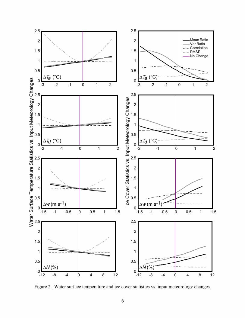
We assessed model sensitivity to boundary condition meteorology (air temperature, humidity, wind speed, and cloud cover) by using each boundary condition (meteorological input) time se-ries with systematic changes along the entire time series in a range determined by its historical maximum and minimum, but maintaining the integrity of the other inputs. First, we investigated the effect on calibration statistics for water surface temperature and ice cover. Figure 2 summa-rizes these statistics. The water surface statistics are best at the original (unchanged) meteorol-ogy; this is hardly surprising since this data were used in the model calibrations. Any changes in any of the meteorology variables (air temperature, aT , dew point temperature, dT , wind speed, w , or cloud cover, N ) decrease the correlation, increase the RMSE, and cause the mean ratio and variance ratio to deviate from unity. Ice cover shows a similar behavior except that the best values of all calibration statistics do not occur simultaneously nor at the unchanged data abscissa as they do for water surface temperature statistics. This is expected since the calibrations used minimization of RMSE for water surface temperatures rather than RMSE for ice cover for eight of the ten model parameters. Also, of the two remaining parameters, for which a minimization of ice cover was used to calibrate, only one has any effect. The calibrations are not sensitive to

aτ . Therefore, water surface temperature statistics were much closer to optimum values than were ice cover statistics in the calibrations with the original (unchanged) meteorology. It ap-pears from Figure 2 that 1°C decreases in air temperature or dew point temperature improve ice cover RMSE, correlation, and mean ratio, at the expense of the variance ratio. Likewise, in-creases in wind speed or cloud cover improve ice cover RMSE, correlation, and mean ratio. Limited increases in wind speed and cloud cover also benefit ice cover variance ratio.

Modeled water surface temperature, heat in storage, lake evaporation, and ice cover were calcu-lated for every day of the 1950-1999 period by using calibrated model parameters. The seasonal average (average for every day of the calendar year across the entire 50 years of simulation) was plotted against day of the year. This was repeated for each of several values of boundary condi-tion meteorology from the range determined by historical maximums and minimums. For exam-ple, surface water temperatures are plotted for various air temperature perturbations in Figure 3; there are similar plots for the other model outputs for each model input but they are not shown here for the sake of brevity. The top panel in Figure 3 shows the seasonal water surface tempera-ture distribution across the annual cycle as a function of eight perturbations of air temperature ( aT ). The middle panel shows the difference between each seasonal distribution and the base distribution (calculated with aT + 0.00°C). The bottom panel shows a ratio, obtained by dividing each value in the middle plot by the corresponding perturbation from the base value. This repre-sents the sensitivity of the seasonal distribution to changes in the model input meteorology ( aT in this example). The bottom panel in Figure 3 is useful for determining if the sensitivity of a model output is linear with changes in a model input variable. If it is linear, then all of the curves collapse to a single seasonal distribution. Sensitivity plots similar to the one in the bot-tom of Figure 3 were created for each of the constant changes in boundary condition meteorol-ogy. Figure 4 shows the sensitivity of seasonal water surface temperature, seasonal stored heat, daily lake evaporation, and ice cover to the four meteorology-variable-changes. Note that all model outputs appear to have sensitivity that is approximately linear to changes in boundary condition meteorology changes, as evidenced by the near collapse of all curves in the plots of

6

Figure 2. Water surface temperature and ice cover statistics vs. input meteorology changes.

0

0.5

1

1.5

2

2.5

-3 -2 -1 0 1 20

0.5

1

1.5

2

2.5

-3 -2 -1 0 1 2

Mean RatioVar RatioCorrelationRMSENo Change

0

0.5

1

1.5

2

2.5

-2 -1 0 1 20

0.5

1

1.5

2

2.5

-2 -1 0 1 2

0

0.5

1

1.5

2

2.5

-1.5 -1 -0.5 0 0.5 1 1.50

0.5

1

1.5

2

2.5

-1.5 -1 -0.5 0 0.5 1 1.5

0

0.5

1

1.5

2

2.5

0

0.5

1

1.5

2

2.5

Wat

er S

urfa

ce T

empe

ratu

re S

tatis

tics

vs. I

nput

Met

eoro

logy

Cha

nges

Ice

Cov

er S

tatis

tics

vs. I

nput

Met

eoro

logy

Cha

nges

∆T (°C)a ∆T (°C)a

∆T (°C)d ∆T (°C)d

∆w (m s )-1 ∆w (m s )-1

∆N (%)-12 -8 -4 0 4 8 12 -12 -8 -4 0 4 8 12

∆N (%)

7

Figure 4. This appears most especially pro-nounced for seasonal evaporation for all me-teorology changes and for all model outputs for dew point temperature changes. It ap-pears least pronounced for seasonal stored heat for changes in air temperature or wind speed. All meteorology changes appear to affect seasonal water surface temperature most during the summer months but affect stored heat the least during the springtime. Of course, ice cover is affected most during the winter months.

It is difficult to compare the sensitivity of two model outputs to changes in one mete-orology variable or the sensitivity of one model output to changes in two meteorology variables since units of sensitivity are gener-ally not similar. (The exceptions are com-parisons of the sensitivity of one model out-put to changes in air temperature and dew point temperature.) However, by consider-ing the expected range or standard deviation of meteorology variables, it is possible to make comparisons of sensitivity across model outputs or meteorology changes. Since we have evidence of approximately linear relationships in Figure 4 between model outputs and changes in meteorology variables, it is appropriate to consider the daily average sensitivity, computed by aver-aging over all meteorology changes each day of the annual cycle. The median over the annual cycle of the daily average sensi-tivity is then considered as a representative index of sensitivity. (In the case of ice cover, only January through April is used to compute medians). By multiplying the me-dian sensitivity for a model output by the historical standard deviation of a meteorology variable, we have a generalized measure of the impact of a changed meteorology variable on a modeled output that considers the expected range of the variable. Dividing by the standard deviation of the respective model output further nor-malizes results; these normalized indices are then comparable between both model outputs and meteorology changes. They are summarized in Table 1.

Ice Cover: It is clear that air temperature is the most significant meteorological input variable affecting ice cover; see Table 1. The negative sign for air temperature and dew point tempera-

Figure 3. Seasonal water temperature sensitiv-ity to changes in air temperature.

Seasonal Temperature (°C)

Seasonal Temperature Difference (°C)

Seasonal Temperature Sensitivity (°C / °C)

0

4

8

12

16

J F M A M J J A S O N D

+2.13°C+1.60°C+1.07°C+0.53°C+0.00°C-0.71°C-1.42°C-2.13°C-2.84°C

-5

-3

-1

1

3

5

J F M A M J J A S O N D

0

0.5

1

1.5

2

2.5

3

J F M A M J J A S O N D

8

0123 0123 -3-2-10 -3-2-10

-0.10

0.1

0.2

0.3

0.4

0.5

-0.10

0.1

0.2

0.3

0.4

0.5

0.6

-0.5

-0.4

-0.3

-0.2

-0.10

0.1

-0.6

-0.5

-0.4

-0.3

-0.2

-0.10

0.1 J

FM

AM

JJ

AS

ON

DJ

FM

AM

JJ

AS

ON

D

Seasonal Lake Heat Storage Sensitivity

Seasonal Surface Water Temperature Sensitivity

+2.1

3°C

+1.6

0°C

+1.0

7°C

+0.5

3°C

-0.7

1°C

-1.4

2°C

-2.1

3°C

-2.8

4°C

∆Ta

(°C /

°C)

(10

cal

/°C

)19

∆Ta

(°C /

°C)

(10

cal

/°C

)19

+1.6

7°C

+1.2

5°C

+0.8

4°C

+0.4

2°C

-0.4

9°C

-0.9

8°C

-1.4

6°C

-1.9

5°C

∆Td

∆Td

(°C /

(m s

))-1

+1.0

7+0

.80

+0.5

4+0

.27

-0.2

9-0

.58

-0.8

7-1

.16

m s

-1

m s

-1m

s-1

m s

-1m

s-1

m s

-1

m s

-1m

s-1

∆w

∆w

-1(1

0 c

al /

(m s

))19

(°C /

(10%

))(1

0 c

al /

(10%

))19

∆N +10% +8

%+5

%+3

%-3

%-5

%-8

%-1

0%

∆N

-1

-0.6

-0.20.2

0.6 -1

-0.6

-0.20.2

0.61 -1

-0.6

-0.20.2

0.61 -1

-0.6

-0.20.2

0.61

-30

-20

-100

-30

-20

-100 0102030 0102030

Seasonal Daily Lake Evaporation Sensitivity

Seasonal Ice Cover Sensitivity

(mm

/°C

)(%

/°C

)

+2.1

3°C

+1.6

0°C

+1.0

7°C

+0.5

3°C

-0.7

1°C

-1.4

2°C

-2.1

3°C

-2.8

4°C

∆Ta

∆Ta

∆Td

+1.6

7°C

+1.2

5°C

+0.8

4°C

+0.4

2°C

-0.4

9°C

-0.9

8°C

-1.4

6°C

-1.9

5°C

∆Td

(mm

/°C

)(%

/°C

)

(mm

/ (m

s))

-1(%

/ (m

s))

-1

∆w+1

.07

+0.8

0+0

.54

+0.2

7-0

.29

-0.5

8-0

.87

-1.1

6

m s

-1

m s

-1m

s-1

m s

-1m

s-1

m s

-1

m s

-1m

s-1

∆w

(mm

/ (1

0%))

(% /

(10%

))

∆N

∆N +10% +8

%+5

%+3

%-3

%-5

%-8

%-1

0%

JF

MA

MJ

JA

SO

ND

JF

MA

MJ

JA

SO

ND

Figu

re 4

. Se

ason

al m

odel

out

put s

ensi

tiviti

es to

bou

ndar

y co

nditi

on m

eteo

rolo

gy v

aria

ble

chan

ges.

9

Table 1. Model output median sensitivities, ψ , and normalized median sensitivity indices, θ .

Meteorology Variableb Model Output Variablea aT dT w N

(1) (2) (3) (4) (5)

January through December

Standard Deviation, σ̂ • ˆaTσ = 11.18 °C ˆ

dTσ = 11.06 °C ˆwσ = 1.38 m s-1 ˆ Nσ = 25.09 %

T median sensitivity, ,Tψ • ( ˆTσ = 4.61 °C)

0.48 °C / °C

0.31 °C / °C

-0.65 °C / (m s-1)

-0.057 °C / %

, ,T Tθ ψ• •= × σ̂ • / ˆTσ 1.16 0.74 -0.19 -0.31

H median sensitivity, ,Hψ •

( ˆHσ = 1.59×1019 cal.) 2.5

1018 cal / °C 1.8

1018 cal / °C -2.9

1018 cal / (m s-1) -0.39

1018 cal / %

, ,H Hθ ψ• •= × σ̂ • / ˆHσ 1.76 1.25 -0.25 -0.61

E median sensitivity, ,Eψ • ( ˆEσ = 1.26 mm)

0.09 mm / °C

-0.02 mm / °C

-0.05 mm / (m s-1)

-0.021 mm / %

, ,E Eθ ψ• •= × σ̂ • / ˆEσ 0.80 -0.18 -0.05 -0.42

I Median Sensitivity, ,Iψ • ( ˆ Iσ = 15.78 %)

-14.43 % / °C

-9.05 % / °C

20.40 % / (m s-1)

1.39 % / %

, ,I Iθ ψ• •= × σ̂ • / ˆ Iσ -10.2 -6.34 1.78 2.21

June through August

Standard Deviation, σ̂ • ˆaTσ = 3.36 °C ˆ

dTσ = 3.67 °C ˆwσ = 0.99 m s-1 ˆ Nσ = 23.64 %

T Median Sensitivity, ,Tψ • ( ˆTσ = 4.14 °C)

1.07 °C / °C

0.77 °C / °C

-1.65 °C / (m s-1)

-0.215 °C / %

, ,T Tθ ψ• •= × σ̂ • / ˆwTσ 0.87 0.68 -0.39 -1.23

aT = water temperature, H = lake heat content, E = lake evaporation, and I = ice cover. b

aT = air temperature, dT = dew point temperature, w = wind speed, and N = cloud cover.

ture normalized median sensitivity indices ( , aI Tθ and , dI Tθ , respectively) indicate that as air and dew point temperatures decrease, ice cover increases. Air temperature is an important parameter affecting latent and sensible heat transfer between the lake surface and the atmosphere. Decreas-ing dew point temperature reflects lower humidity, which increases evaporation and increases heat loss from the lake, which, in turn, increases ice cover. Wind speed and cloud cover have a much smaller impact on ice cover as indicated by their normalized indices ( ,I wθ and ,I Nθ , re-

10

spectively). The positive sign for wind speed and cloud cover indices indicates positive changes in these meteorological inputs result in increases in ice cover. At first, it may seem puzzling that an increase in cloud cover would increase ice cover, since an increase in cloud cover corresponds to an increase in net long-wave radiation to the lake surface, which would increase heat in the lake and decrease ice cover. However, the incident solar radiation, iQ , is a function of cloud cover also; as used by the model,

( )0.355 0.68 1iQ X N = + − (6)

where X = cloudless-day insolation. An increase in cloud cover decreases incident short-wave radiation to the lake surface. The net effect is a general reduction in heat input to the surface, lowering the surface temperature and increasing ice cover. An increase in wind speed corre-sponds to an increase in lake mixing volume and lowering of surface temperature, which results in greater ice cover. However, in a deep lake with a large surface area, such as Lake Superior, the effects of ice dynamics and lake hydrodynamics can be important contributing factors (e.g., upwelling of warmer waters), reducing ice cover extent. The evaporation model does not include these effects, resulting in the observed relatively small impact of wind speed.

Water Temperature: Water temperature increases as air and dew point temperatures increase and decreases as wind speed and cloud cover increase. It is sensitive, in decreasing order of im-portance, to air temperature, dew point temperature, cloud cover, and wind speed, respectively; see the normalized median sensitivity indices, ,Tθ • , for January through December in Table 1. Water temperature sensitivity to meteorological inputs, ,Tψ • , is largest in magnitude in June, July, and August, the months when summer stratification is established, as illustrated in Figures 3 and 4; compare the median sensitivities, ,Tψ • , in Table 1 for the two periods January through December and June through August. However, because the standard deviations of the meteorol-ogy variables are smaller during June through August than they are during January through De-cember, the normalized median sensitivity indices, ,Tθ • , do not reflect the increased sensitivity of water temperature to air or dew point temperatures. Likewise, the influence of wind speed and cloud cover on water temperature is greater in June, July, and August then in the rest of the year, as reflected by both the median sensitivities ( ,T wψ and ,T Nψ ) and the normalized median sensi-tivity indices ( ,T wθ and ,T Nθ ). In fact, for June through August, cloud cover and not air tempera-ture is the most important normalized index in Table 1. It is followed by air temperature, dew point temperature and wind speed in that order. In the summer, radiation dominates the surface energy budget and as cloud cover decreases, solar radiation increases by (6) and so does surface water temperature, despite the decrease in net long-wave radiation into the lake. As wind speed increases, surface temperature decreases due to an increase in the mixing volume. As air temperature increases, so does water temperature, as a result of increased sensible heat transfer to the water. Similar results are observed for dew point temperature, since increases in dew point represent increases in humidity or decreases in evaporative capacity of the overlying air. As evaporation drops with increasing dew point temperature, cooling of the lake is reduced and water temperature rises.

11

Evaporation: Of the four meteorological inputs, evaporation is most sensitive to air tempera-ture; see the normalized median sensitivity indices, ,Eθ • , in Table 1. Positive air temperature changes produce increased evaporation with the largest seasonal sensitivity to air temperature in the winter (see Figure 4) when there is maximum evaporation on large Lake Superior. (Lake Superior has maximum stored heat then coupled with cold dry air moving over the warm water.) Evaporation is next most sensitive to cloud cover; increasing cloud cover contributes to long-wave radiation additions to the lake and produces increased evaporation. Evaporation sensitivity to dew point temperature is seasonal, being positive during the winter and slightly negative dur-ing the fall; see Figure 4. (This is one of only three cases where model output sensitivity is not uniformly positive or negative throughout the annual cycle; the other two are discussed subse-quently.) During most of the year when sensitivity is positive, positive changes in dew point temperature reduce evaporation (high dew point implies increased humidity and decreased lake evaporation). A secondary effect, of dew point on emissivity, dominates during the fall however, giving rise to the negative sensitivity shown in Figure 4. Emissivity is a function of vapor pres-sure in the air and is given as ( )1 20.53 0.065 ae+ in (3). Then, positive changes in dew point temperature imply increased humidity and emissivity which result in increased net long-wave radiation (and heat) into the lake, thereby increasing evaporation in excess of what is lost by de-creased vapor pressure difference between the water and the air. Annual sensitivity to dew point temperature in Table 1 is much smaller than that for air temperature because of the seasonal re-versal of the impact of dew point temperatures on evaporation. The response of evaporation to wind speed represents a second case where model output sensitivity changes sign seasonally; see Figure 4. During the period October through January, positive wind speed changes increase evaporation, but during the period February through September, decrease evaporation. The negative sensitivity results because of wind-induced mixing in the lake; higher wind speeds in-crease ice cover, thereby reducing evaporation during the winter, and increase the depth of the mixed layer during the summer, thereby lowering surface temperature and evaporation then. Thus, as was the case with dew point temperature, the annual sensitivity of evaporation to wind speed in Table 1 is relatively small because of its seasonal reversal.

Heat Storage: Lake heat storage is relatively less sensitive to input meteorology during the win-ter months because of the formation of ice cover which impedes energy and mass (water vapor) transfers between the lake and atmosphere. Heat storage is most sensitive to changes in air tem-perature followed by changes in dew point temperature; see the normalized median sensitivity indices, ,Hθ • , in Table 1. Positive air temperature changes produce positive heat storage changes except during February and March for some of the lower temperatures changes; see Figure 6. This is the third case where model output sensitivity changes sign seasonally. During most of the year, for all of the temperature changes investigated here, increases in air temperature add heat to the lake. During February and March, for the lowest temperature changes, increases in air temperature decrease ice cover, which allows increased evaporation and other surface heat loss, thereby lowering the heat stored in the lake. Cloud cover changes have the next largest im-pact on lake heat storage. Reduced cloud cover results in increased heat storage because of in-creases in solar radiation at the lakes surface [see (6)], which is apparently larger than the net long-wave radiation losses [see (3)] on an annual basis. Finally, negative changes in wind speed results in less latent and sensible heat loss to the atmosphere and increases in heat storage.

12

SUMMARY

The calibration statistics for surface water temperatures are best at the unchanged meteorology (Figure 2) while decreases in aT or wT and increases in wind speed and cloud cover improve some of the ice cover calibration statistics. This is because calibrations use minimization of root mean square error for water temperature, rather than for ice cover, for eight of the ten model pa-rameters. The sensitivity of model outputs to changes in meteorology is approximately linear (Figure 4). There are changes in the sensitivity of model outputs over the annual cycle, e.g. sur-face water temperatures are affected by model inputs most during the summer, and ice cover most during the winter. Ice cover is the most sensitive, of the four model outputs considered here, to each meteorology variable (has the highest absolute normalized median index value,

,Iθ • ), followed by lake heat content, surface water temperature, and evaporation, in that order; evaporation is slightly more sensitive than surface water temperature to cloud cover. The annual normalized indices for aT and wT are larger than those for w and N (Table 1) for the units used in this study. Thus, errors in observed values (in the same units) of these two model inputs might have a relatively larger impact on model outputs, all other things being equal. The evaporation model is a 1-dimensional (1-D) model; 2-D and 3-D process models might produce different sen-sitivities to model outputs. This is expected for wind speed; the 1-D model considered here, showed only a small impact of wind speed on ice cover. Finally, synergistic effects of consider-ing perturbations of two or more inputs on model outputs, while beyond the scope of this study, should be explored.

ACKNOWLEDGMENT

This is Great Lakes Environmental Research Laboratory contribution no. 1236.

REFERENCES

Croley, T. E., II, 1989. Verifiable evaporation modeling on the Laurentian Great Lakes, Water Resources Research, 25(5):781-792.

Croley, T. E., II, 1992. Long-term heat storage in the Great Lakes, Water Resources Research, 28(1):69-81.

Croley, T. E., II, 1994. Hydrological impacts of climate change on the Laurentian Great Lakes, Trends In Hydrology, Council of Scientific Research Integration, Research Trends, Kaitha-mukku, Trivandrum, India, 1:1-25.

Croley, T. E., II, and R. A. Assel, 1994. A one-dimensional ice thermodynamics model for the Laurentian Great Lakes, Water Resources Research, 30(3):625-639.

Gill, A. E., and J. S. Turner, 1976. A comparison of seasonal thermocline models with observa-tion, Deep Sea Research, 23:391-401.

Kraus, E. B., and J. S. Turner, 1967. A one-dimensional model of the seasonal thermocline II, The general theory and its consequences, Tellus, 19:98-105.

Lofgren, B. M., F. H. Quinn, A. H. Clites, R. A. Assel, and A. J. Eberhardt, 2000. Water Re-sources. In: Preparing for a Changing Climate: the Potential Consequences of Climate Variability and Change, Peter J. Sousounis and Jeanne M. Bisanz (Editors). University of Michigan, Ann Arbor, Michigan, pp. 29-37.